The INFLUX network – eddy covariance in and around an urban environment

The eddy covariance method is used by various disciplines to measure atmospheric fluxes of both vector and scalar quantities. One long-term, multi-site urban flux network experiment was the Indianapolis Flux Experiment (INFLUX), which successfully deployed and operated eddy covariance towers at eleven locations for varying deployment periods, measuring fluxes from land cover types within and surrounding the urban environment in Indianapolis, Indiana, USA. The data collected from this network of towers have been used to quantify urban greenhouse gas, energy, and momentum fluxes, assess the performance of numerical weather and carbon cycle models, and develop new analysis methods. This paper describes the available data associated with the INFLUX eddy covariance network, provides details of data processing and quality control, and outlines site attributes to assist in data interpretation. For access to the various data products from the INFLUX eddy covariance work, please see the data availability section below. For access to the various data products from the INFLUX eddy covariance work, please see Table 5 in the data availability section.

1 Introduction

Eddy covariance (EC) is a method for quantifying atmospheric fluxes of mass, energy, and momentum. EC measurements are commonly used to infer the exchange of these quantities between the Earth's surface and the atmosphere. Using EC, investigators can monitor a system with minimal disturbance over long periods, making it an attractive method for various disciplines (e.g., ecologists, meteorologists, hydrologists) (Baldocchi et al., 2001). The technique is based on sampling the spectrum of turbulent eddies and their associated scalar constituents to calculate the covariance between the vertical wind component and the variable of interest. This covariance can be used to quantify the turbulent surface flux of a variable (vector or scalar) in many conditions (e.g. Yi et al., 2000). The EC method typically uses fast-response (≥ 10 Hz) instruments to measure three-dimensional wind and various atmospheric scalars (e.g., CO₂, H₂O, temperature). A comprehensive description of the EC method can be found in Aubinet et al. (2012) and Burba (2013) or many micrometeorological-focused texts (Foken, 2008; Lee et al., 2004).

Recent studies have employed an increasing number of EC measurements to study surface-atmosphere fluxes across cities (Lipson et al., 2022; Nicolini et al., 2022). Nicolini et al. (2022) compared thirteen EC towers in eleven different European cities to assess the impacts of the COVID-19 lockdown on CO₂ emissions. They found a significant relationship between factors such as the lockdown stringency index (e.g., the Oxford Stringency Index) and the relative change in CO₂ flux (i.e., before vs. during lockdown), demonstrating the value of EC measurements for detecting both long- and short-term changes in CO₂ fluxes in real time. Jongen et al. (2022) used evapotranspiration measurements from EC towers across twelve cities to infer water storage capacity. Their results show both variability in inferred storage across the analyzed sites and a substantial difference between the estimated storage in urban areas and storage reported in rural environments. The Urban-PLUMBER project (https://urban-plumber.github.io/, last access: 2 April 2025) gathered measurements from twenty flux towers located all over the world, creating a dataset of urban EC measurements covering a spectrum of different climatic conditions and urban forms, and has used these data for urban land surface model evaluation (Lipson et al., 2022). Other large-scale efforts, such as the ICOS-Cities project, are expanding the number of EC measurements in the urban environment. The FLUXNET project continues to bring together EC data into a globally-accessible database.

Interpreting EC measurements in the urban environment is inherently difficult due to the high level of heterogeneity (e.g., thermal and aerodynamic). This difficulty is not limited to EC but also applies to many traditional micrometeorological theories and methods developed primarily for horizontally homogeneous settings where, for example, horizontal spatial derivatives in the governing equation can be assumed negligible. One approach to address this heterogeneity is to require deployments in seemingly homogeneous urban areas where, for example, the EC flux footprint (i.e., the upwind area measured by the EC system) envelops an area of roughly uniform surface characteristics and scalar source distributions (Turnbull et al., 2025). When possible, this greatly simplifies data interpretation. This approach also severely limits the number of viable EC measurement locations, most of which are seldom representative of an urban mosaic, which, as stated, is often heterogeneous.

A contrasting and complementary approach is to deploy EC flux measurements in heterogeneous settings and to adapt our analysis methods and theories to the inherently heterogeneous nature of the urban environment. At least two issues emerge in this scenario. First, the EC flux measurements cannot be interpreted in terms of a single set of land surface characteristics. EC measurements collected in heterogeneous environments should be construed (at the very least) as a function of wind direction and atmospheric stability conditions, ideally with a flux footprint model (e.g., Horst and Weil, 1992; Kljun et al., 2015), and combined with data sets that can describe the urban landscape at a resolution that is finer than the flux footprint. Such data analysis is complicated by the fact that typical flux footprint models (e.g., Horst and Weil, 1992; Kljun et al., 2015) were developed for horizontally homogeneous environments and should therefore be used with caution in highly heterogeneous systems.

Second, heterogeneity is ubiquitously associated with surface discontinuities, which are well understood to give rise to rapidly evolving, non-equilibrium flow features such as internal boundary layers and secondary circulations. Furthermore, in most real-world urban scenarios, these flow features merge and interact, further complicating the problem (Bou-Zeid et al., 2020). For example, a secondary circulation driven by spatial roughness or thermal differentials can result in non-negligible horizontal flux divergence or mean advection (Feigenwinter et al., 2012), violating the one-dimensional, vertical transport, which is typically used to infer surface-atmosphere exchange from EC flux measurements (Aubinet et al., 2012; Burba, 2013). Diagnosing the presence of such flows can be attempted, for example, with multi-level turbulent flux measurements (Yi et al., 2000). Yi et al. (2000) found only modest deviations from vertical-only transport in a highly heterogeneous forested region. In other locations, however, heterogeneity-induced secondary circulations have also been shown to impact EC measurements in arguably less complex settings (compared to an urban setting) like agricultural fields (Eder et al., 2015a) and deserts (Eder et al., 2015b), and have been linked to the lack of closure of the surface energy balance endemic to EC flux measurements (Mauder et al., 2020). In summary, surface-atmosphere fluxes inferred from EC flux measurements collected in heterogeneous urban environments should also be used with attention to the inherent challenges and limitations.

Mixed sources further complicate the interpretation of urban EC flux measurements, as biological and anthropogenic factors are often intertwined. The combined impacts of anthropogenic and biogenic sources and sinks of CO₂ (Miller et al., 2020; Turnbull et al., 2019), sensible and latent heat (Ward et al., 2022), and momentum (Kent et al., 2018) are measured by urban EC instruments. This complexity builds on underlying mixtures of fluxes within natural (e.g., respiration [both heterotrophic and autotrophic] and photosynthesis) and anthropogenic (e.g., vehicles and buildings; residential and industrial) systems. Heterotrophic respiration of CO₂ by people should be approximately 0.24 µmol m⁻² s⁻¹ using population densities for Indianapolis reported in the 2020 United States census (948 people km⁻²) and an average respiration rate of 942 gCO₂ person⁻¹ d⁻¹ (Prairie and Duarte, 2007).

None of these challenges, however, are new or unique to urban systems, and all can be addressed through ongoing research. Airborne EC has been conducted over heterogeneous flux footprints for decades (Desjardins et al., 1992; Oncley et al., 1997), and flux footprint decomposition methods have been employed for nearly as long (Schuepp et al., 1990; Mahrt et al., 2001). Footprint decomposition has been used with tower-based EC to study natural (Wang et al., 2006; Xu et al., 2017) and anthropogenic (Dennis et al., 2022; Wu et al., 2022) fluxes. Biological and anthropogenic CO₂ fluxes have been disaggregated in the urban environment using both statistical partitioning methods (Crawford and Christen, 2015; Lee et al., 2021; Menzer and McFadden, 2017) and tracer ratio methods (Ishidoya et al., 2020; Wu et al., 2022). Complex ecosystem flux sites (e.g., Davis et al., 2003) have served as a guide for flux upscaling studies (Wang et al., 2006; Xiao et al., 2014), and all sites in the Americas flux tower network (Ameriflux, Novick et al., 2018) have been categorized according to their degree of heterogeneity (Chu et al., 2021). Lateral flow in low turbulence conditions has been recognized as a problem in all EC deployments (Barr et al., 2013). Landscape-scale secondary circulations have been investigated in agricultural (Kang et al., 2007) and forested landscapes (Butterworth et al., 2021). Given that urban environments are where over 55 % (and rising) of the global population lives (Sun et al., 2020) and given the past successes in studying complex micrometeorological environments, we would like to stress the importance of understanding these complex systems and moving ahead with measurements that go beyond the classic homogeneous flux tower site.

Many efforts have successfully measured fluxes using EC in the urban environment (Biraud et al., 2021; Kotthaus and Grimmond, 2014; Menzer and McFadden, 2017; Vogt et al., 2006; Wu et al., 2022). Urban greenhouse gas (GHG) emissions are a common focus of these efforts. Urban areas are responsible for 67 %–72 % of anthropogenic CO₂ emissions globally (Lwasa et al., 2023). Many cities have pledged to reduce GHG emissions amid anthropogenic climate change, for example, initiatives like NetZeroCities (European Union, 2025) or the Covenant of Mayors (Kona et al., 2018). The EC method can directly measure GHG fluxes within the tower's footprint and reveal the urban metabolism. Liu et al. (2012) investigated spatial and temporal variability of CO₂ fluxes in the Beijing megacity using the EC method and found weekly (e.g., traffic volume) and seasonal (e.g., domestic heating) patterns in CO₂ fluxes. Crawford and Christen (2015) were able to disaggregate observed CO₂ fluxes into biogenic and anthropogenic sources by modeling various sources/sinks within the turbulent source area (i.e., flux footprint) of a residential area in Vancouver, Canada. Similar work by Stagakis et al. (2019) disaggregated measured CO₂ fluxes in the Mediterranean city of Heraklion, Greece, using source-area modeling and high-resolution geospatial descriptions of the surrounding urban areas, finding high overall annual emissions compared with other EC-derived estimates from other cities. Pawlak and Fortuniak (2016) assessed the temporal variability of CH₄ fluxes in a populated area of Łódź, Poland, and found the city's annual emissions were comparable to surrounding natural sources like wetlands. Menzer and McFadden (2017) used statistical partitioning of CO₂ fluxes over a suburban neighborhood outside Saint Paul, Minnesota to separate biogenic from anthropogenic sources.

Recently, intra-urban networks have begun to emerge. Multiple towers within and outside a single city enable a more detailed understanding of the urban system than could be achieved with a single flux tower. For example, Nicolini et al. (2022) were able to use paired towers within the same city (e.g., residential vs. non-residential) to infer qualitative information on the dominant CO₂ driver (e.g., vehicular, vegetation, etc.). Peters et al. (2011) showed the benefit of measuring turfgrass lawns using a short-stature (1.35 m) tower to help interpret evapotranspiration (ET) measurements made on the collocated KUOM tower (40 m) in Saint Paul, Minnesota. In recent years there has been an expansion of urban EC in the United States through projects like the Indianapolis Flux Experiment (INFLUX, Davis et al., 2017), the Baltimore Social and Environmental Collaborative (BSEC), the Coastal Rural Atmospheric Gradient Experiment (CoURAGE, Davis et al., 2024), the Community Research on Climate and Urban Science (CROCUS, Raut et al., 2025), and the Southwest Urban Integrated Field Laboratory (Zweig, 2025).

INFLUX was a contribution to the urban greenhouse gas test beds program of the National Institute of Standards and Technology (Semerjian and Whetstone, 2021). This program endeavored to “improve emission measurement tools to better equip decision makers and mitigation managers with capabilities to chart progress in GHG emissions mitigation” (https://www.nist.gov/greenhouse-gas-measurements/urban-test-beds, last access: 2 April 2025). The INFLUX project was the longest-running test bed in this program. Atmospheric inversions were the primary technological approach employed for urban GHG emissions estimates in the test bed program (Karion et al., 2023; Lauvaux et al., 2020; Yadav et al., 2023), given their ability to encompass emissions from the entirety of an urban area. Atmospheric inversions struggle, however, to infer the spatial structure of emissions within a city (e.g. Lauvaux et al., 2020). EC flux towers, long used to study fluxes at a spatial resolution more accessible to local-scale, process-based model evaluation, have been deployed in INFLUX to complement whole-city atmospheric inversions.

The INFLUX EC flux towers measured CO₂, H₂O, energy, and momentum fluxes in and around Indianapolis. The network included EC flux observations from eleven locations (Fig. 1), comprising over a decade and a half of observation site years (Table 1, Fig. 2). These tower locations range from agricultural sites in the croplands surrounding Indianapolis to towers in the cities' interior over turfgrass, suburban forests, residential areas, and heavily developed urban regions (Fig. 1). This multiplicity of flux sites was achieved by moving instrumentation from site to site as deemed necessary to sample the variability in fluxes in and around this urban landscape. A subset of the flux measurements (Table 1) have been co-located with mole fraction observations (Richardson et al., 2017) from the INFLUX urban GHG testbed monitoring network (Miles et al., 2017a).

Table 1 Site identification in FLUXNET format, deployment period, and a short description of each site.

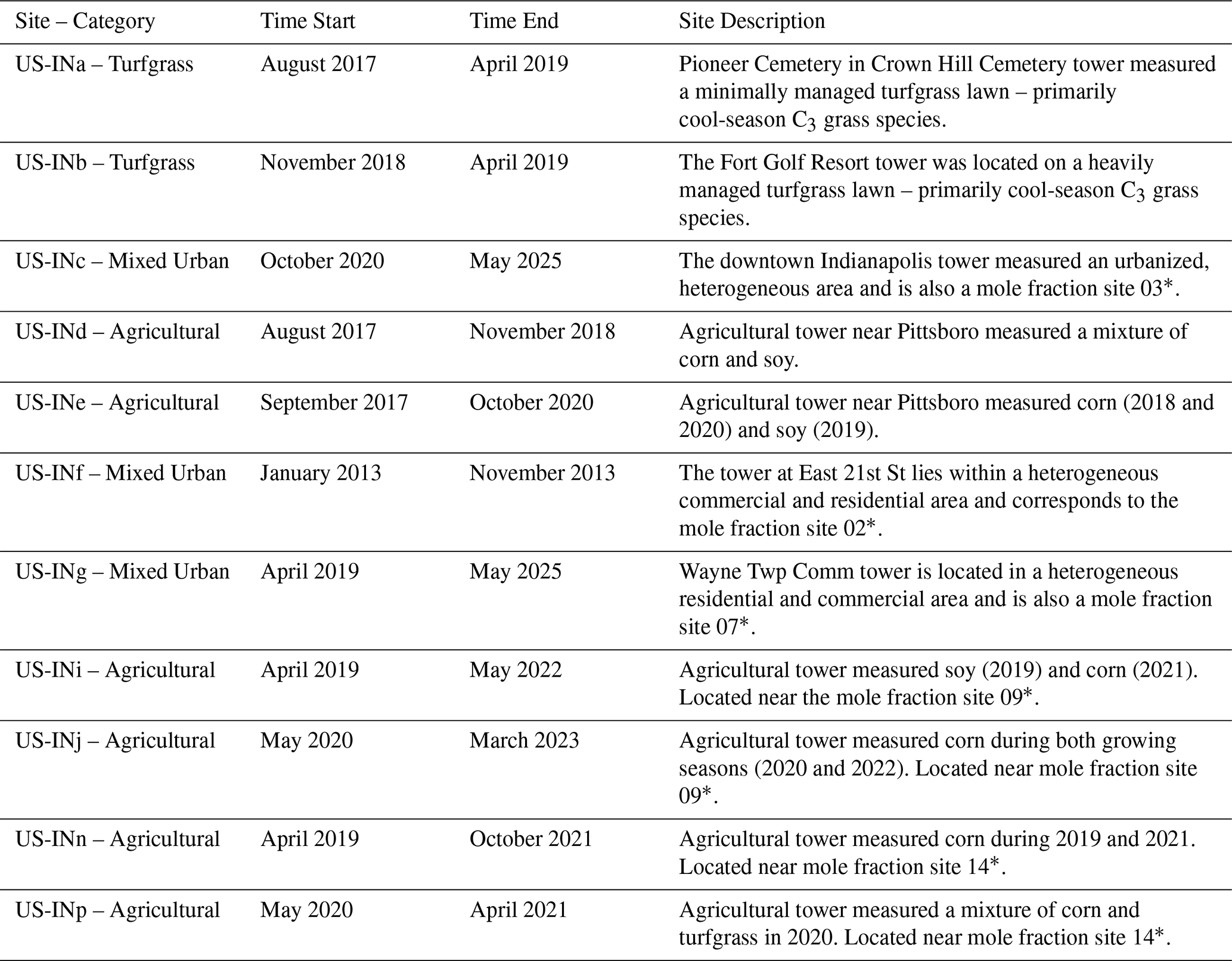
^* Mole fraction towers and their numbers are described in Miles et al. (2017a).

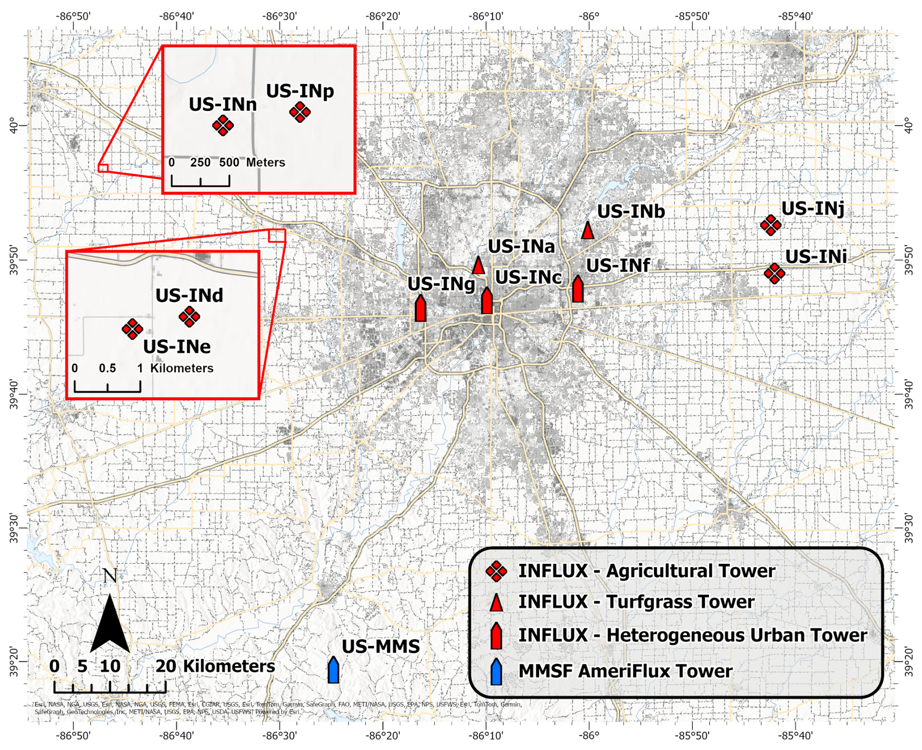
Figure 1 Locations of INFLUX eddy covariance towers in and around Indianapolis, IN. Specific flux tower site locations (i.e., latitude and longitude) are included in the site metadata file with the processed data files. The gray shading represents the 2023 impervious surface cover from the National Land Cover Database (Dewitz, 2021). Major roadways are depicted in light yellow, and waterways are shown in light blue. The Morgan-Monroe State Forest (MMSF) AmeriFlux tower is also included for spatial reference. Service layer credits go to City of Indianapolis, Marion County, Esri, TomTom, Garmin, SafeGraph, FAO, METI/NASA, USGS, EPA, NPS, USFWS, and GeoTechnologies Inc | Powered by Esri.

Figure 2 Data availability at each site through the timeline of the INFLUX project. Each half-hour data point is indicated by a red “+”, flux instrumentation deployment dates are indicated by black x's, and flux instrumentation decommissioning dates are indicated by gray x's. Any missing data between the deployment and decommissioning dates is due to power loss or instrument malfunction.

This paper documents the urban EC measurements undertaken as part of the INFLUX project. We discuss methods for quality-controlling the INFLUX EC measurements and describe the groups of EC flux sites within the INFLUX project (i.e., agricultural, turfgrass, and heterogeneous urban towers). We present the data processing required to interpret the data within this urban network and document the availability of data products.

2 INFLUX Eddy Covariance Tower Network

2.1 General Climate

The INFLUX project is based in and around Indianapolis, IN, USA. The city of Indianapolis and the surrounding area are on the boundary of two Köppen climate classifications, Dfa and Cfa (Kottek et al., 2006) at an elevation of approximately 220 m above sea level. We reference data from the National Oceanic and Atmospheric Administration's (NOAA) National Centers for Environmental Information (NCEI) to provide averages for the period between 1991 and 2025. Indianapolis receives, on average, approximately 111 cm of liquid precipitation and 65 cm of snowfall (depth) annually. The annual average daily high and low temperatures are 17 and 7 °C, respectively.

2.2 Flux tower sites and site categories

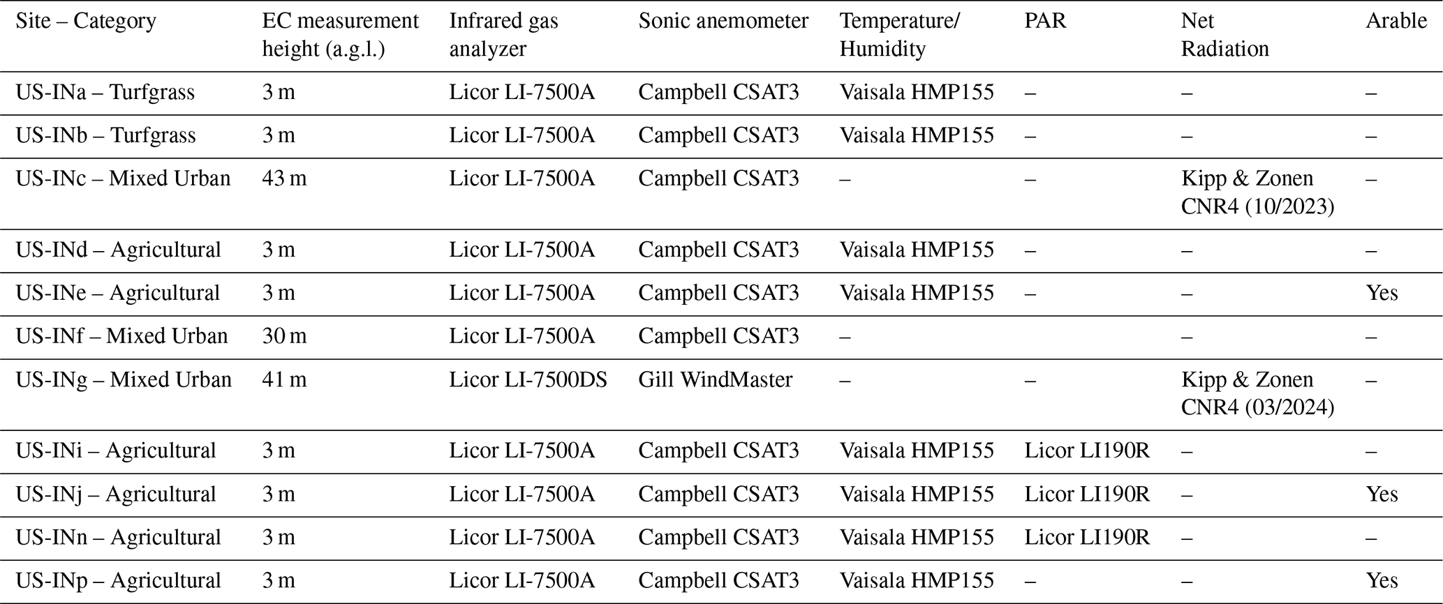
The INFLUX flux towers can be subdivided into heterogeneous (US-INc, US-INg, US-INf) and homogeneous sites. Within the homogeneous grouping, we further subdivide the towers into agricultural (US-INd, US-INe, US-INi, US-INj, US-INn, US-INp) and turfgrass (US-INa, US-INb) categories. Each site is equipped with a sonic anemometer, either a Gill WindMaster (WindMaster, Gill Instruments, Lymington, UK) or CSAT3 (CSAT3, Campbell Scientific, Logan, UT, USA), and an infrared gas analyzer (LI-7500DS or LI-7500A, LI-COR Biosciences, Lincoln, NE, USA) collecting data at 10 Hz frequency (Table 2). The low-stature towers are also equipped with a temperature and humidity probe (HMP155, Vaisala Oyj, Vantaa, Finland), and a subset of them are equipped with photosynthetically active radiation (PAR) sensors (LI190R, LI-COR Biosciences, Lincoln, NE, USA) (Table 2). US-INc and US-INg were equipped with 4-way net radiometers (CNR4, Kipp and Zonen, Delftechpark, Netherlands) in October 2023 and March 2024, respectively. In addition to the INFLUX EC towers, the AmeriFlux Core Site US-MMS (Fig. 1), located in the Monroe-Morgan State Forest, is approximately seventy kilometers to the southwest of Indianapolis (Dragoni et al., 2011; Schmid et al., 2000).

Table 2 Measurement heights of deployed eddy covariance instruments and flux instruments for each site.

2.3 Data acquisition and organization

The INFLUX EC instruments produce continuous time-series measurements, which are separated into individual GHG data files (.ghg) containing 30 min of continuous data, for a total of 48 files per day. Each GHG file is transferred from the logger to a Linux server using the Secure Socket Shell (SSH) file transfer protocol. Each instrument has a unique incoming directory where the files are stored. Every night, a set of shell scripts checks to see if all 48 files have been delivered. Furthermore, every night, GHG files are copied to an archive while the data files are checked for (i) readability for further processing (occasionally some files are corrupt), (ii) monotonic time increase of recorded data (will be automatically corrected if possible), (iii) any non-ASCII characters which could cause problems during further scientific processing), (iv) incomplete data rows. Emails are automatically generated if any fault is recognized, while copies of the automatically modified and corrected data files are saved. Each step is captured in a log file. Missing data, errors, and file modifications due to errors trigger an email notification. These checks test file integrity and data completeness. Once the integrity tests are completed, the data is automatically processed and analyzed using EddyPro (LI-COR, 2021) and a set of Python scripts. Graphics of the processed data (a two-week data window) are automatically updated online, allowing for manual monitoring of the incoming data and quick identification and resolution of issues. This allows researchers to quickly determine whether the instruments produce reasonable results or require immediate attention.

2.4 Flux processing and quality control

The complete time series of fluxes is calculated separately from the automatic processing script using a set of distinct post-processing steps and the EddyPro software package. For a comparison between EddyPro and other commonly used software (e.g., TK3 and eddy4R) when processing fluxes at heterogeneous urban flux towers, please see Lan et al. (2024). For every thirty minutes, we apply a block-averaging detrending (Foken, 2008; Lee et al., 2004) and planar fit coordinate rotation (Lee et al., 2004; Paw U et al., 2000; Wilczak et al., 2001). The Vickers and Mahrt (1997) despiking procedure is performed before calculating fluxes, spikes are removed, and the number of spikes is reported. As the molar densities are measured by open-path sensors (LI-7500A or LI-7500DS), we apply the Webb, Pearman, and Leuning correction for density fluctuations (Lee and Massman, 2011; Paw U et al., 2000; Webb et al., 1980) following the iterative methodology employed in EddyPro. The cospectra are corrected (high and lowpass) via the analytical methods of Moncrieff et al. (1997), which is based on the methods of Moore (1986) using the similarity-based cospectral models from Kaimal et al. (1972). For each averaging period, using the methods of Vickers and Mahrt (1997), a set of flags is generated based on the high-frequency measurements. The deployment at Site US-INf was a preliminary effort that did not follow these same procedures. We employed a locally written EC code (Shi et al., 2013) that includes planar fit rotation and Vickers and Mahrt (1997) despiking algorithms. Due to differences in the data acquired for this system, we were unable to apply the data processing used for the remaining INFLUX towers. The US-INf data are described in more detail in Sarmiento et al. (2017) and Wu et al. (2022).

Flux data are flagged for violating an angle of attack test if > 10 % of the wind vectors exceed an attack angle of > |30°| for the averaging period. In the urban environment, the attack angle can be used to examine the impact of wake turbulence generated by roughness elements (RE) within the tower's footprint. For example, wind directions from the southwest (180–225°) of Site US-INc (Fig. 3) are flagged ≥ 30 % of the time, detecting wake turbulence generated by a 30 m tall building 100 m southwest of the tower. From these impacted wind directions, the measured fluxes are not within the inertial sublayer (i.e., the constant flux layer), where traditional EC assumptions are potentially valid.

Figure 3 Percent of total data (i.e., all wind directions) flagged (radial) as a binary attack angle flagging (red/blue) vs. wind direction (angular) at US-INc (October 2020–January 2023). Radial scales show 1.1 %, 2.2 %, 3.3 %, 4.4 %, and 5.6 % of the total data moving from the inner to the outer ring, respectively. The red triangle represents the location of US-INc. The base map is a digital surface map generated using 2016 Indiana Statewide 3DEP LiDAR Data Products for Marion County (USGS, 2018). Service layer credits go to Maxar and Microsoft.

Fluxes are also flagged using a suite of quality control tests available through EddyPro, which are commonly used in EC research. Stationarity tests are conducted for each half-hour using the methodology of Foken and Wichura (1996) and Vickers and Mahrt (1997). Modeled integral turbulence characteristics from flux variance similarity theory are compared to measured variances of winds and scalars using the methods of Foken and Wichura (1996). Depending on the degree of nonstationarity and deviation from flux similarity theory, as determined by the Foken and Wichura (1996) tests, each averaging period is assigned a value (1–9) based on the scheme of Mauder and Foken (2004). When comparing measurements made at the heterogeneous urban towers to similarity predictions, it is worth noting that aerodynamic parameters, such as displacement height, are often directionally dependent (Kent et al., 2018). Thus, the similarity-based relationship should scale differently depending on the wind direction. Subtle details, such as these, are not included in the current version of EddyPro, but the software's default flags, generated (as discussed here), can still guide users in interpreting the data.

For two agricultural sites, US-INn and US-INp, periods of the high-frequency data were lost, and only a version of the processed thirty-minute data using the default EddyPro settings was recovered. At US-INn, the period is from 21 April 2019, 00:00 UTC to 10 January 2020, 03:30 UTC, and at US-INp, it is from 23 May 2020, 21:30 UTC to 22 December 2020, 16:00 UTC. For these periods when high-frequency data were lost, fluxes are calculated using a double-coordinate rotation and flagged according to a simplified version of the 1–9 scheme, as outlined in the Spoleto agreement of 2004 for CarboEurope-IP, as described in Mauder and Foken (2004). These periods of missing high-frequency data have been combined with those where the high-frequency data is available, resulting in a mixture of flagging schemes and coordinate rotation in some columns.

After calculating half-hourly fluxes, additional screening methods generate flags for periods with weak gas-analyzer signals, extreme flux values, or inadequate mechanical mixing during nocturnal periods. The data are flagged if the signal strength reported by the gas analyzer over a half-hour period falls below the mean signal strength for a two-week moving window. Nighttime data (i.e., periods when the solar altitude is ≤ 0°) are flagged during low-turbulence periods using the methods of Goulden et al. (1996). We acknowledge that the use of friction velocity filters in urban areas is still under question (Papale et al., 2022); a consensus has not been reached. We assert that this remains a valuable screening tool for these datasets. Finally, the flux data are flagged based on a threshold of N standard deviations from the mean, where N is a site-specific number chosen to keep flux magnitudes within geophysical limits. While the standard deviation and signal strength flag perform well at identifying potentially erroneous flux calculations, it should be noted that these quality control procedures are imperfect (as with any of the quality control methods mentioned) and could flag legitimate flux measurements.

We provide processed, half-hourly flux datasets for each of the eleven INFLUX sites through Penn State Data Commons and Ameriflux (see Sect. 3). Included with these data are metadata files with information on details such as flagging thresholds (e.g., friction velocity threshold) or site geographic coordinates. We do not remove data based on the generated flags for the data set available on Penn State Data Commons; instead, we leave the filtering decisions to the users. For most use cases, we do not recommend eliminating all points flagged using the quality control flags provided by the methods of Vickers and Mahrt (1997) and Mauder and Foken (2004), as a large proportion of physically reasonable data is flagged. We give an example of four different quality control flag combinations for CO₂, latent heat, sensible heat, and momentum fluxes using observations at Site US-INg in Fig. 4. The four quality control flag combinations for each of these fluxes are summarized in Table 3. We recommended at minimum filtering the data according to friction velocity and CO₂ flux standard deviation flags for analysis of CO₂ fluxes, sensible heat standard deviations flags for analysis of sensible heat fluxes, latent heat standard deviation flags for analysis of latent heat fluxes, and removing wind directions from which the measurement is impact by distortion due to the tower (for Site US-INg, observations from wind directions 30–135° should be removed) for momentum fluxes (Set 1 in Table 3). From wind directions where the towers distort the flow, we do not observe a clear impact on scalar fluxes; thus, we leave the decision for removal to the data user. To remove additional outlier points, we suggest filtering by Sets 2 or 3 (Table 3) as shown in Fig. 4b and c for CO₂ fluxes, Fig. 4f and g for sensible heat fluxes, Fig. 4j and k for latent heat fluxes, and Fig. 4n and o for momentum fluxes. Given the significant reduction of overall data points, we do not suggest the flagging combination of Set 4, as shown in Fig. 4d, h, l, and p, unless the application of the data requires the strictest turbulence screening, which is appropriate only if the most idealized conditions for EC flux measurements are needed. At the heterogeneous urban flux towers (US-INc and US-INg), we recommend not removing scalar flux data based on the Vickers and Mahrt (1997) higher-moment statistics (i.e., skewness and kurtosis), as these flags commonly target realistic data at these sites (Järvi et al., 2018). This is due to the spatial and temporal heterogeneity of the urban environment, which can cause the distribution of high-frequency scalar measurements for a single period often to exceed the default skewness or kurtosis thresholds in EddyPro.

Table 3 Description of quality control flag combinations considered for CO₂, sensible heat (H), latent heat (LE), and momentum (τ) fluxes. The hard flag is abbreviated as “hf” in the table.

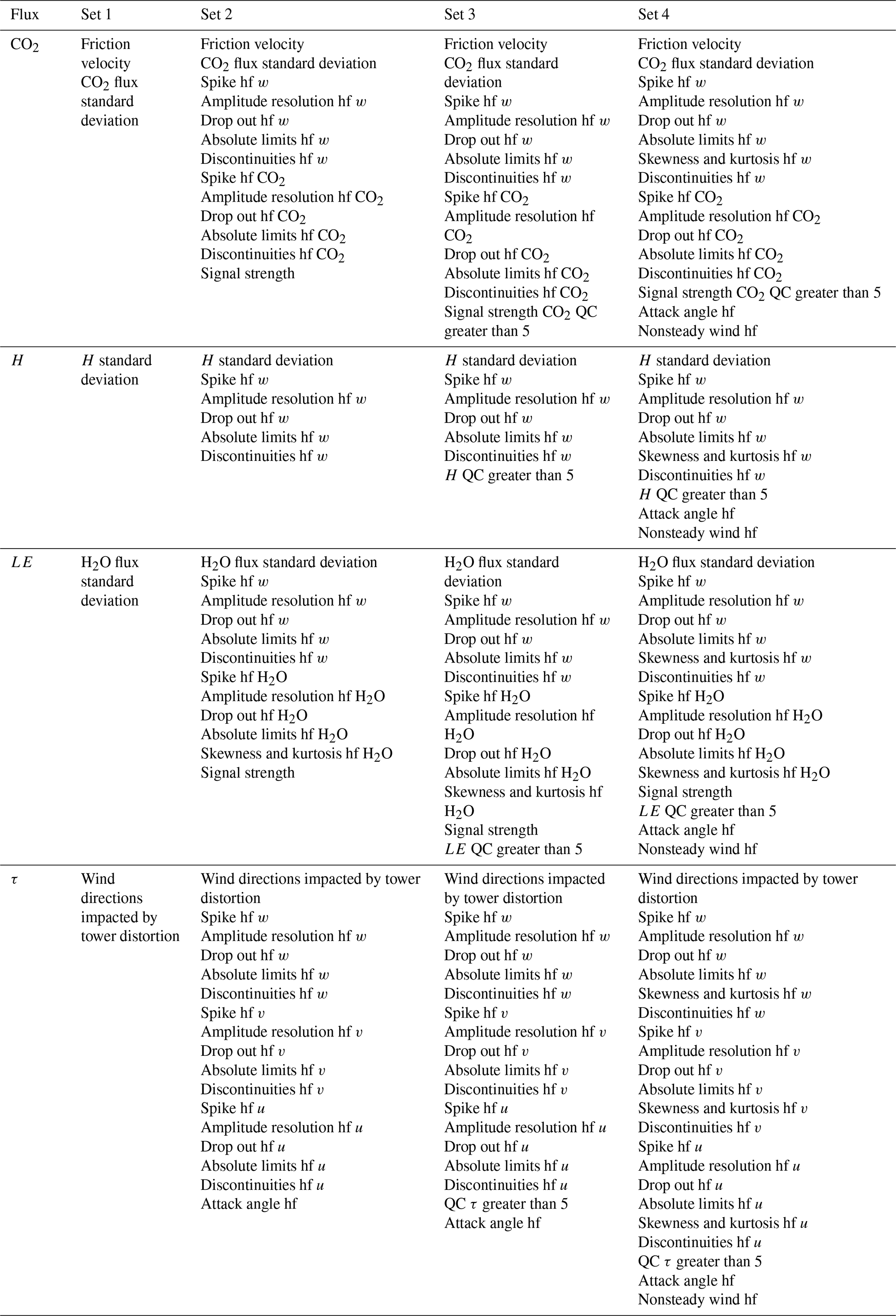
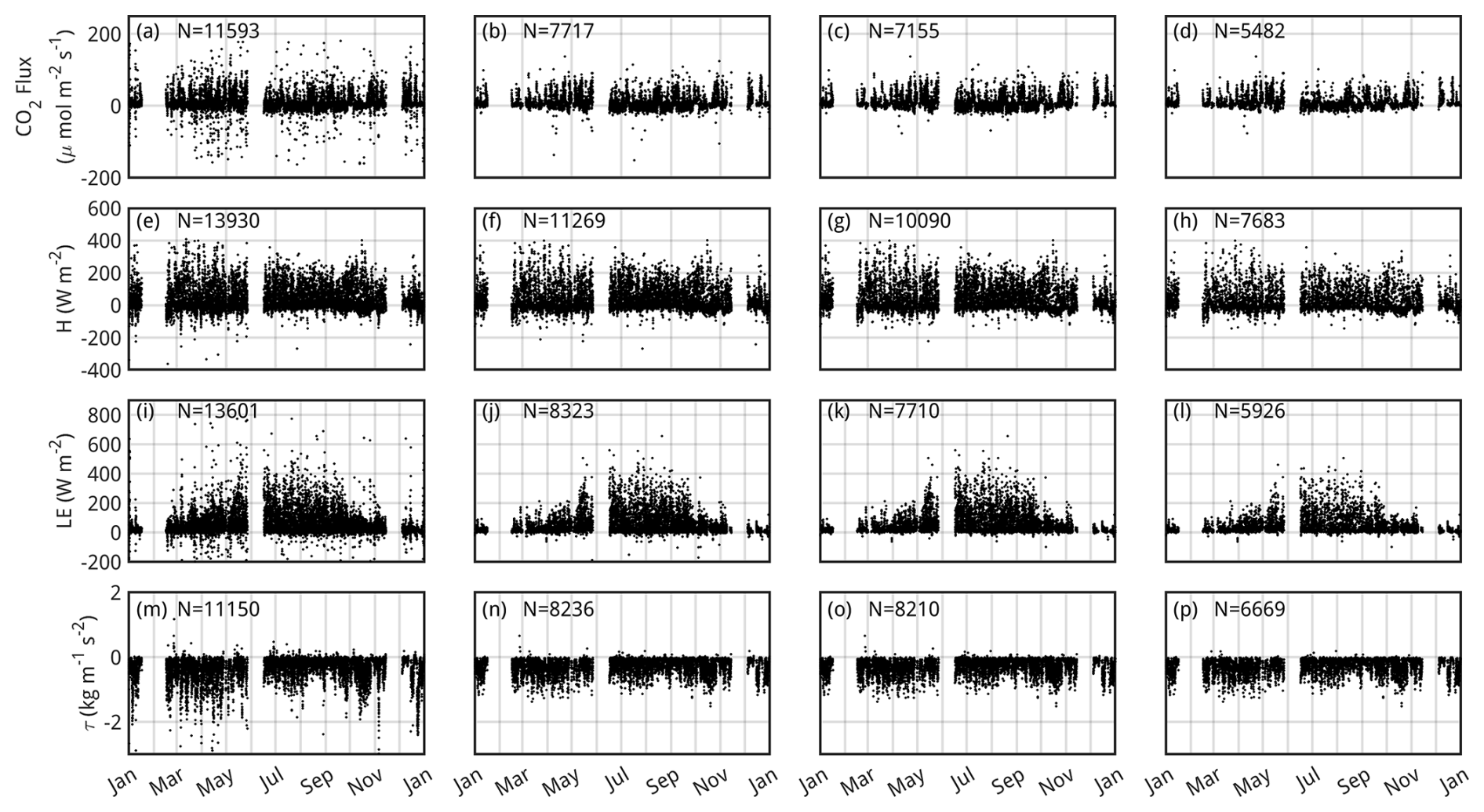
Figure 4 CO₂ fluxes (a–d), sensible heat fluxes (H) (e–h), latent heat fluxes (LE) (i–l), and momentum fluxes (τ) (m–p) at Site US-INg for 2022 with different quality control flags applied. From left to right, the filtering sets 1, 2, 3, and 4 (see Table 3 for full set descriptions) are shown for each of the fluxes, representing a range of filtering choices from least to most stringent. The number of points remaining in the dataset after removing quality control flags is indicated on each panel. With no filtering applied, there are 13 779 CO₂ flux data points, 13 969 sensible heat data points, 13 697 latent heat flux data points, and 13 969 momentum flux data points. For filtering Sets 1, 2, 3, and 4, respectively, 84.1 %, 56.0 %, 51.9 %, and 39.7 % of the total CO₂ flux data are preserved, 99.7 %, 80.6 %, 72.2 %, and 55.0 % of sensible heat flux data are preserved, 99.2 %, 60.7 %, 56.2 %, and 43.2 % of latent heat flux data are preserved, and 79.8 %, 58.9 %, 58.7 % and 47.7 % of momentum flux data are preserved.

2.5 Agricultural Sites

Understanding the boundary layer dynamics and CO₂ fluxes surrounding a city is important for understanding measurements collected within the city. The area surrounding Indianapolis is mainly composed of agricultural fields planted with a rotation of corn and soybeans. We deployed short-stature (∼ 3 m a.g.l.) flux towers at six locations in agricultural fields within 30–60 km of downtown Indianapolis (Fig. 1). The instrumentation for the agricultural sites was, in most cases, relocated annually to sample a variety of fields (specifically US-INd, US-INe, US-INn, US-INp). Each location was given a different site key. We collected data at the six agricultural sites for eleven growing seasons (Fig. 5).

Figure 5 The average summer (JJA) diel cycle of CO₂ fluxes for each agriculture site-year. Each column is also labeled with the surrounding vegetation. The numbers indicate the average half-hour flux for each underlying color.

Flux footprint analyses are used to identify averaging periods when these agricultural towers may have been strongly influenced by vegetation other than the crops to be sampled. These conditions arise from the practical limitation of placing the flux towers close to, but not directly within, the actively managed fields, meaning that at times the towers were located at the boundary between two adjacent crop types. The fractional coverage of the agricultural crop of interest (corn or soybean) within the estimated tower footprint was calculated for each agricultural flux site in the INFLUX network. The calculated fractional coverage values allow a data user to select thresholds for which they would consider the half-hourly flux value representative of the vegetation of interest. The Flux Footprint Prediction (FFP) model, developed by Kljun et al. (2015), is utilized to calculate the vegetation fraction for each point in the data record. Atmospheric boundary layer heights for input into the FFP come from ERA5 reanalysis (Hersbach et al., 2023). Imagery from Google Earth and ArcGIS Pro software is used to visually select areas covered with the vegetation of interest. Areas with the vegetation type of interest are assigned a value of one, while other areas are assigned a value of zero. For all half hours during which the required input data are available, the FFP climatology function simulates footprints at a 1 m grid spacing for a 501 m by 501 m domain. The site map distinguishing landcover types and the footprint estimate is multiplied to obtain a gridded map representing only the footprint attributable to the vegetation of interest. For every possible half hour, two values are computed using the predicted footprints: a value representing the footprint attributable to the vegetation of interest and a value for the total footprint. The former is calculated by summing over the footprint attributable to the vegetation of interest, and the latter by summing the footprint over the entire domain. The ratio of these values represents the fraction of the footprint attributable to the vegetation of interest.

The agricultural EC measurements have been used to evaluate the background conditions for the city. Murphy et al. (2025) evaluated the accuracy and precision of a simple carbon flux model used to describe ecosystem CO₂ fluxes surrounding the city. Ongoing work is evaluating the latent and sensible heat fluxes simulated by numerical weather prediction (NWP) models. These models are necessary for conducting urban climate and GHG inversion studies.

2.6 Turfgrass Sites

Turfgrass is a common urban land cover (Milesi et al., 2005). Only a handful of towers have previously been deployed to measure turfgrass lawns (i.e., mixed species low-stature vegetation often artificially managed through irrigation, fertilization, and/or mowing) (Ng et al., 2015; Pahari et al., 2018; Pérez-Ruiz et al., 2020; Peters and McFadden, 2012) despite these lawns being an abundant vegetative community in urban areas (Horne et al., 2025a). We deployed two flux towers (US-INa and US-INb) to monitor turfgrass lawns. The two INFLUX turfgrass towers captured different levels of management intensity. US-INa measured fluxes over a cemetery lawn (Fig. 6) with lower intensity management (i.e., infrequent mowing, no fertilization, and no irrigation), and US-INb measured fluxes over a golf course (i.e., frequent mowing, fertilization, and irrigation). These towers were of low stature and sited to minimize contributions to the flux footprint from anything other than turfgrass. We have used the CO₂ flux data from these two turfgrass towers to evaluate the Vegetation Photosynthesis and Respiration Model (VPRM) performance at reproducing seasonal turfgrass fluxes, finding that these lawns require a unique representation in the VPRM (Horne et al., 2025a).

Figure 6 The average winter (DJF) (a) and summer (JJA) (b) diel cycle of latent heat (LE), sensible heat (H), and CO₂ fluxes for US-INa (cemetery lawn). Data for averaging are taken from the periods over the site deployment (August 2017–April 2019). The dashed and dashed-dot horizontal lines indicate zero crossings for the CO₂ or sensible and latent heat flux, respectively.

2.7 Heterogeneous Footprint (Mixed) Urban Flux Towers

Three communications towers with EC instrumentation at 30 to 43 m a.g.l. were instrumented to measure fluxes from the complex, mixed land cover typical of urban environments. These higher-altitude measurements are necessary to measure fluxes above the trees and buildings commonly found throughout the metropolitan area. As mentioned, these towers host flux instrumentation and mole fraction measurements that are part of the INFLUX urban GHG testbed monitoring network (Miles et al., 2017a; Davis et al., 2017). In addition, publicly available high-resolution data, although not included here, are available and can complement specific investigations, aiding users in interpreting measurements. Footprint climatologies generated using the Kljun et al. (2015) FFP model for the INFLUX mixed urban flux towers are shown in Fig. 7. We include footprint climatologies for these sites alone to show the level of heterogeneity at each site and the estimated area measured by these towers. These footprint climatologies guide our characterization of the regions sampled by these towers. We describe broad characteristics of the urban landscapes in their flux footprints following the example of the Urban-PLUMBER project (https://urban-plumber.github.io/, last access: 2 April 2025, Lipson et al., 2022). Table 4 provides metadata for the area surrounding the three heterogeneous urban flux towers (US-INc, US-INf, US-INg). In Table 4, values for roughness length (z₀) and displacement height (z_d) are provided. These length scales are simultaneously fitted using the logarithmic wind profile and isolating measurement periods during near-neutral conditions ($|z/L|<\mathrm{0.05}$, where z is the height of the EC measurement and L is the measured Obukhov length), where the tower frame does not impact the measurement. These provided z_d and z₀ values serve as a reasonable first-order estimate for use in a flux footprint model. It should be noted that data from these towers have been employed in multiple previous studies. Wu et al. (2022) demonstrated a method of disaggregation using INFLUX EC data and mole fraction measurement profiles available at the three INFLUX mixed urban flux towers (Richardson et al., 2017; Miles et al., 2017a), as well as tracer ratio methods. This methodology estimates the fossil fuel component of the CO₂ flux by combining carbon monoxide (CO) flux estimates with measurements of the CO to CO₂ flux ratio from fossil fuel combustion (Turnbull et al., 2015). The biogenic CO₂ flux is then determined by subtracting the fossil fuel flux from the total CO₂ flux measured via EC. Vogel et al. (2024) applied this methodology to the flux record from US-INg to study changes in emissions caused by the COVID-19 lockdown. Both Wu et al. (2022) and Vogel et al. (2024) employed flux footprint and tracer decomposition methods in conjunction to compare the EC measurements with the Hestia urban emissions inventory (Gurney et al., 2012). Kenion et al. (2024) used US-INc EC flux data to demonstrate our ability to infer local-scale urban GHG fluxes using flux-gradient and flux-variance methods. These approaches can be applied to mole fraction measurement sites that are relatively abundant across the NIST urban test beds and other urban GHG mole fraction monitoring programs.

Table 4 Metadata for the surrounding land cover at the three heterogeneous flux towers. We include values of roughness length (z₀) and displacement height (z_d) for each of the towers. The domain is 4 km² centered around the respective tower and separated into quadrants NE [0–90°), SE [90–180°), SW [180–270°), and NW [270–360°) to capture heterogeneity surrounding the tower. Data for percent impervious and canopy fractions come from the National Land Cover Database (NLCD) using data for 2021 (US-INc and US-INg) and 2013 (US-INf) (Dewitz, 2021). LiDAR data used to estimate roughness elements (RE) (buildings and trees ≥ 2 m) characteristics comes from the 2016 Indiana Statewide 3DEP LiDAR Data Products for Marion County (USGS, 2018). Roughness element density is the ratio of surface area occupied by REs to total surface area (i.e., planar area index).

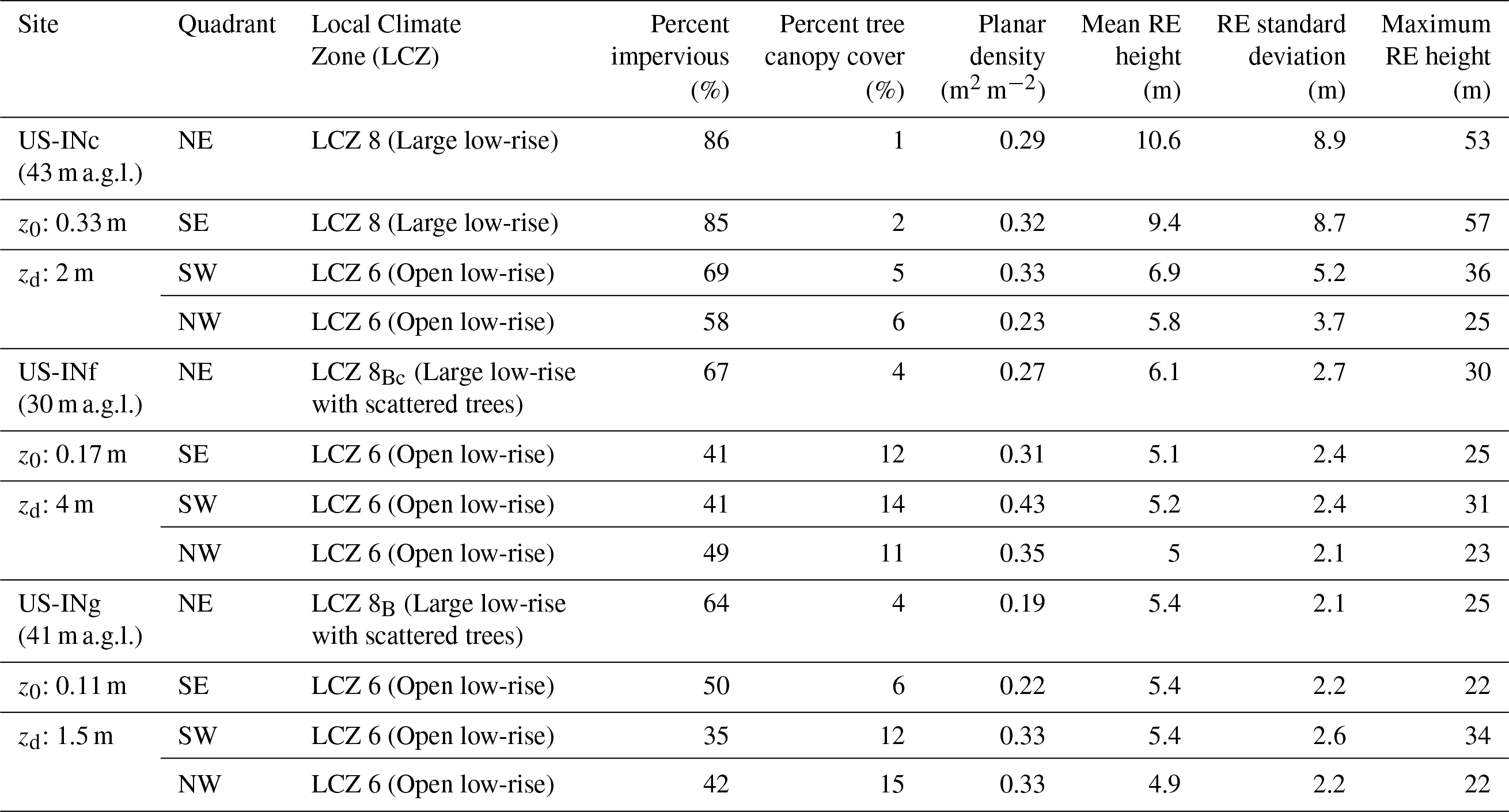
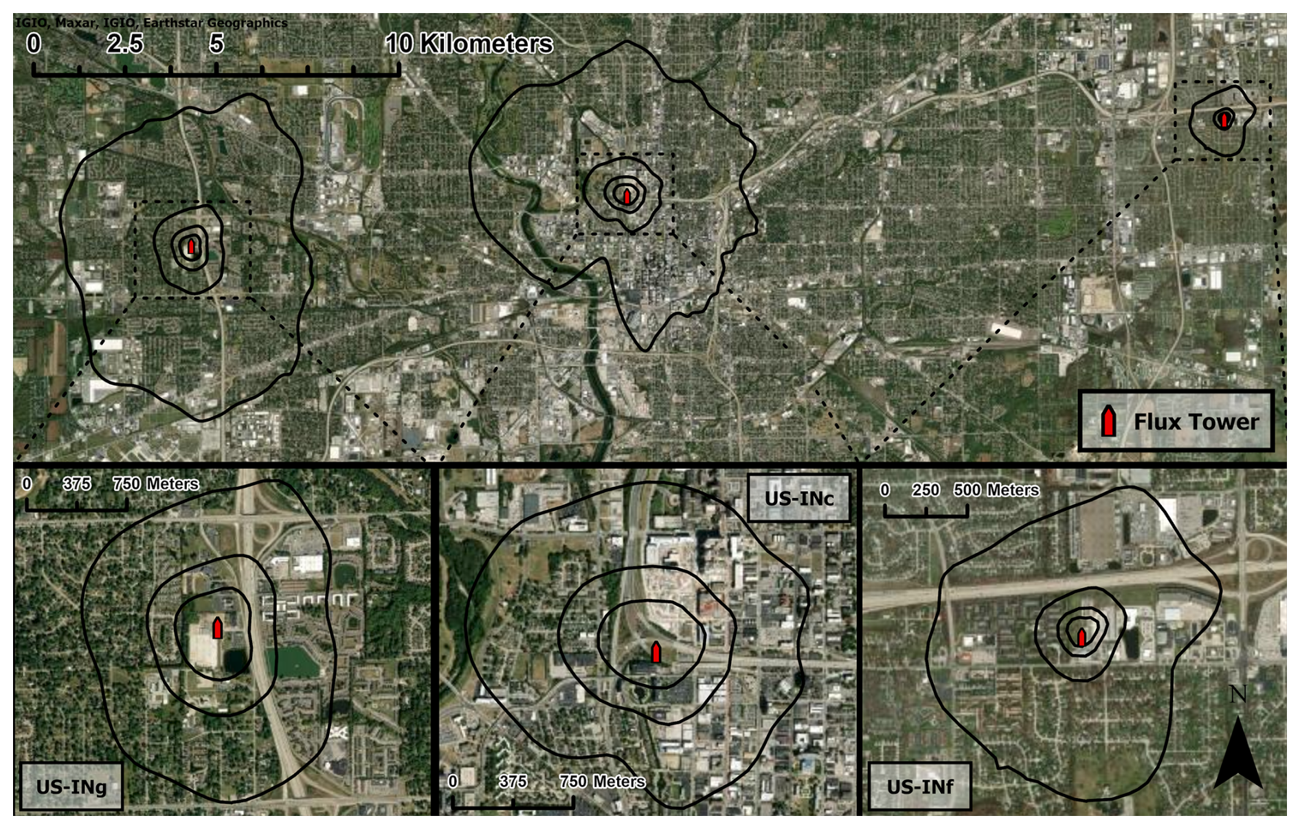
Figure 7 Flux footprint climatologies for all three heterogeneous urban flux towers are shown. Footprint climatologies are created using the Kljun et al. (2015) flux footprint prediction (FFP) model and available data from 2022 (US-INc and US-INg) or 2013 (US-INf). Boundary layer height data for FFP are provided by ERA5 reanalysis. The outermost climatology boundary represents 90 % of the area, and extents moving towards the respective tower represent a 20 % decrease in climatological area (i.e., 70 %, 50 %, 30 %). Wind directions impacted by the building wake (Fig. 2) at US-INc are removed. Zoomed-in maps of the area around each tower are provided, with their extent shown by the dashed outlines on the upper plot. Service layer credits go to Earthstar Geographics, IGIO, and Maxar.

Two mixed urban flux towers, US-INf and US-INg, can each be interpreted as two distinct flux tower sites. We describe these differences in terms of building and vegetation cover (Table 4) and local climate zones (LCZ) (Stewart and Oke, 2012). The EC instruments at US-INg, for example, are set between a highway (LCZ E – Bare rock or paved) and commercial buildings (LCZ 8_B – Large low-rise with scattered trees) to the east and a forested residential neighborhood (LCZ 6 – Open low-rise) to the west. The two sectors exhibit dissimilar diel patterns of CO₂ fluxes (Fig. 8). To the west, we observe a photosynthetic drawdown from the suburban forest during the growing season. To the east, we can observe two distinct peaks in net emissions, corresponding to morning and evening rush-hour traffic (Vogel et al., 2024). Similarly, the footprint at US-INf is roughly divided into northern and southern sectors (Table 4), with highway and commercial areas to the north and residences to the south. Multiple INFLUX studies (Vogel et al., 2024; Kenion et al., 2024; Wu et al., 2022) have shown that the results are highly interpretable using this simple wind direction interpretation.

Figure 8 Isopleths of measured CO₂ flux at US-INg (April 2019–January 2023) as a function of time of year (x axis) and time of day (y axis) for (a) easterly wind directions (0–180°) and (b) westerly wind directions (180–360°). Positive values indicate net emissions of CO₂; negative values indicate a net uptake of CO₂.

We have not divided the flux data from US-INf and US-INg into two distinct records, nor have we posted flux footprint data sets to accompany each flux tower. However, the flux tower records contain all the data needed to subdivide the datasets and produce flux footprints, except for the atmospheric boundary layer height, which can be obtained from reanalysis products such as ERA5 (Hersbach et al., 2023). We note that urban systems frequently violate the assumptions implicit in the surface layer similarity theory and, consequently, the current flux footprint models (e.g., homogeneous turbulence forcing within the flux footprint). We, along with others, such as Feigenwinter et al. (2012), argue that existing footprint models (e.g., Kljun et al., 2015) remain quite helpful in interpreting these datasets. However, more research into the sensitivity of these models to complex urban systems is warranted.

3 Data availability

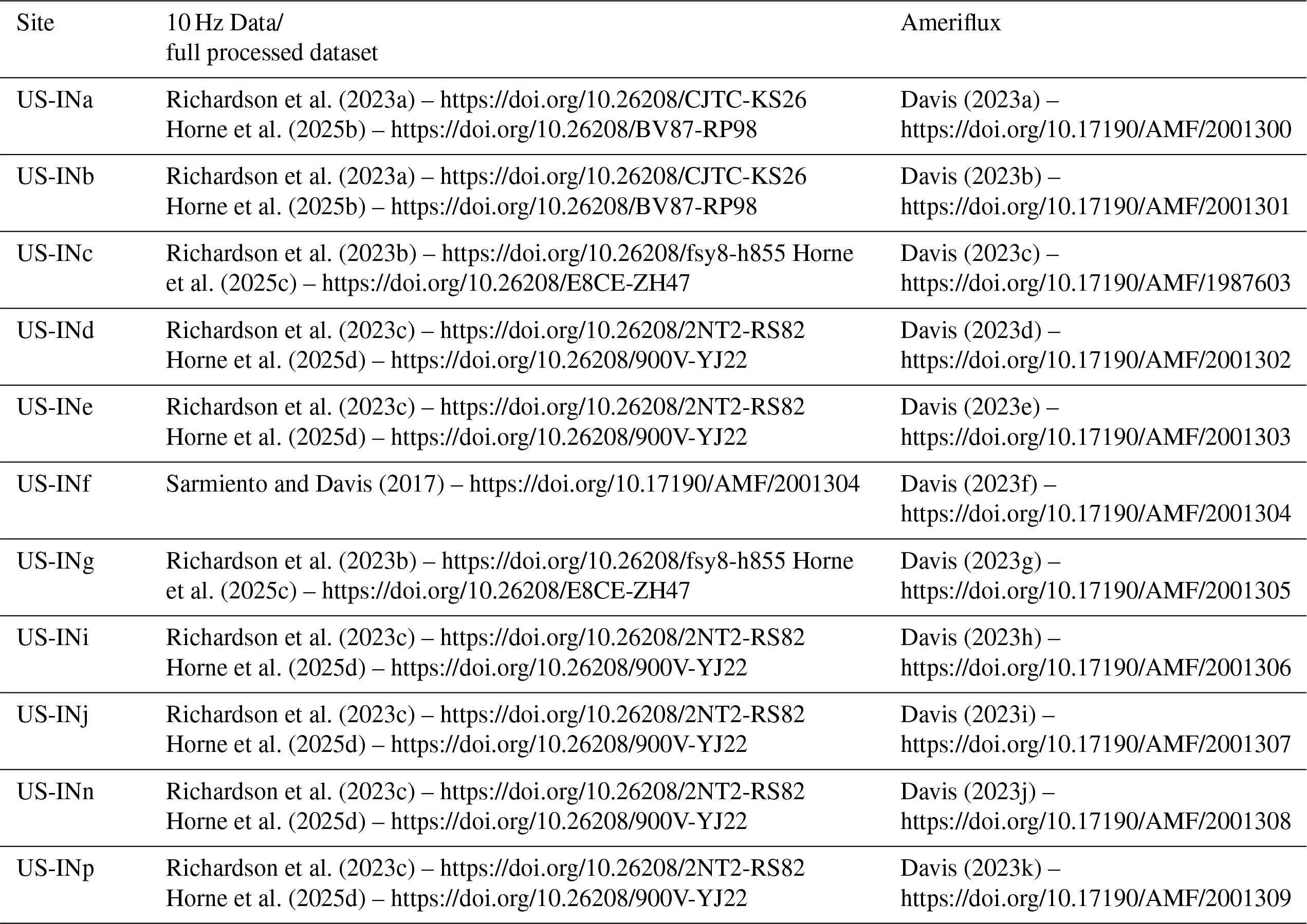
Unprocessed 10 Hz data and processed INFLUX data are available on Penn State Data Commons (Table 5). This version contains all the processed data with flagging, but no data has been removed based on flagging. This processed data also included a metadata file describing the naming convention of variables and flagging. Data from all agricultural sites includes calculated fractional coverage and data collected using the Arable sensors on-site.

In addition, all INFLUX EC datasets are available through the Ameriflux network (https://ameriflux.lbl.gov/, last access: 2 April 2025, Table 5). As of May 2025, the operation of all INFLUX flux towers has concluded. Data collected in 2025 at US-INg and US-INc sites will be processed, updated, and made available through all datasets in Table 5.

These flux measurements were a component of a broader research effort, the Indianapolis Flux Experiment (INFLUX). Multiple additional measurements and model data sets exist, creating a more complete experimental data set to assess urban greenhouse gases in Indianapolis, IN. These include mole fraction measurements (Miles et al., 2017b), flask measurements (https://gml.noaa.gov/dv/site/?stacode=INX, last access: 2 April 2025), Doppler lidar measurements (https://csl.noaa.gov/projects/influx/, last access: 2 April 2025), anthropogenic emissions inventories (Gurney et al., 2018), aircraft measurements (https://influx.psu.edu/influx/data/flight/, last access: 2 April 2025), VPRM simulations (Horne and Davis, 2024; Murphy et al., 2024), and Weather Research and Forecast (WRF) Reanalysis (Deng et al., 2020), which are not described in detail here. For more information concerning the INFLUX Project and the data collected, please visit https://influx.psu.edu (last access: 2 April 2025). Most of these complementary data sets can be found at Penn State's Data Commons.

Table 5 Citations for each INFLUX tower. The raw data collected directly from the instruments, a processed version of the data available on Ameriflux, and a processed version with no flagged data removed are available through Penn State Data Commons.

4 Conclusions

The INFLUX EC network has become a vital component of the multivariate INFLUX data set. Micrometeorological methods like EC can bridge the gap between land surface modeling and atmospheric inverse methods used to quantify urban GHG fluxes. The INFLUX EC flux data expands the growing database of urban flux measurements. Data representative of the range of land-atmosphere fluxes encountered in this region was obtained by deploying multiple sites representative of the land cover of the city and its surroundings. We hope the data availability will support cross-collaboration between projects involving urban environments.