The MAESTRO turbulence dataset derived from the SAFIRE ATR42 aircraft

The MAESTRO airborne field campaign took place between 10 August and 10 September 2024 over the North Atlantic tropical ocean near the Cabo Verde Islands. Its goal was to investigate the processes that control the mesoscale organization of clouds with a payload of probes and sensors, as well as vertically and horizontally-pointing radars and lidars. A particular attention was given to the role of coherent structures in the boundary layer. This focus motivated the acquisition of high-resolution measurements of temperature and water vapor to capture turbulence dynamics in the subcloud layer. To achieve this, six hygrometers and four temperature sensors were deployed, including a new fast-rate hygrometer called FAST-WAVE. This article describes the turbulence dataset, prepared on the basis of these measurements. It consists of 25 Hz segmented time series of calibrated water vapor mixing ratio, temperature, and three-dimensional wind taken with an air speed of approximately 100 m s⁻¹, relative to the aircraft, their corresponding fluctuations, as well as statistical moments, covariance, and integral length scales. In total, 40 h of stabilized legs data were gathered in a wide range of mesoscale contexts and local cloud conditions, with nearly 13 h consisting of high-quality boundary-layer samples. This paper describes the methodological choices required to obtain the dataset, including calibrations, and corrections applied to the original measurements. The collection of NetCDF files composing this dataset is publicly available on the AERIS website (https://doi.org/10.25326/812#v7.0, Jaffeux and Lothon, 2025; see also https://maestro.aeris-data.fr/overview/, last access: 9 June 2026).

1 Introduction

The role of clouds in global climate dynamics remains associated with many mysteries and open questions. The simulation of clouds in numerical models also remains challenging, especially the representation of the diversity and behavior of low-level clouds over the oceans (Konsta et al., 2022). The tropical ocean is populated by many cloud types, ranging from small shallow cumulus to deep convective clouds. Low-level clouds are ubiquitous in this environment and their albedo makes them key players in the energy budget of the Earth (Bony and Dufresne, 2005). These clouds interact with their environment through condensation and evaporation, and by interacting with solar and terrestrial radiation. Using observations, several configurations have been described in the boundary layer with respect to convection, turbulence, and cloudiness. For example, shallow convection has been linked to organized structures in the subcloud layer, such as roll vortices creating cloud streets (LeMone and Pennell, 1976). In another case, the turbulence in the subcloud layer was found to be locally suppressed through cloud precipitation or evaporation while a cold pool formed, enhancing turbulent fluxes in the boundary layer at its front (de Szoeke et al., 2017). In another configuration the boundary layer and clouds above were decoupled (Nowak et al., 2021). Understanding how such scenarios interplay, influence local circulation, contribute to broader cloud organization patterns, and, finally, affect the radiative impact of clouds, relies on the acquisition of representative observations.

Starting with the GATE experiment, scientists have formulated hypotheses about the organization of tropical clouds (Warner et al., 1979). More recently systematic classifications of cloud organization using satellite images have been proposed over the tropical ocean (Stevens et al., 2020; Janssens et al., 2021). Links between the variety of cloud patterns and near-surface wind and stability of the low troposphere were pointed out (Bony et al., 2020) and confirmed by ground based instrumentation over Barbados (Schulz et al., 2021). Data from the EURECA field campaign (Bony et al., 2017 and Bony et al., 2022) were used to understand these different patterns (Bony et al., 2025). Using LES simulation, Dauhut et al. (2023) reproduced and analyzed one case of meso-scale cloud organization observed during EURECA and highlighted the importance of cold pools and mesoscale circulation in its formation. Other LES studies used this dataset to evaluate whether current models are able to reproduce cloud organizations (Schulz and Stevens, 2023; Jansson et al., 2023). As is often the sign of success in scientific research, EURECA answers questions by raising new ones, that have already inspired the community to return to the field and collect new data.

From August to September 2024, a network of international field campaigns, named ORCESTRA (Organized Convection and EarthCARE Studies over the Tropical Atlantic) (Stevens et al., 2025), took place over the tropical Atlantic to investigate the organization of convection, namely MAESTRO (Mesoscale organisation of tropical convection), PERCUSSION (Persistent EarthCare underflight studies of the ITCZ and organized convection) (Groß et al., 2026), BOW-TIE (Beobachtung von Ozean und Wolken – Das Trans ITCZ Experiment), PICCOLO (Process investigation of clouds and convective organization over the tropical ocean), CLARINET (CLoud and Aerosol Remote sensing for EarThcare) (Bell, 2024), CELLO (Cloud and EarthCARE caL/vaL Observations), SCORE (Sub-Cloud Observations of Rain Evaporation), and STRINQS (Soundings and TuRbulent eddy measurements in the ITCZ with a Network of QuadcopterS) projects. A common objective of these campaigns, is to collect relevant observations in the atmosphere in the vicinity of the Inter-Tropical Convergence Zone (ITCZ). These eight research projects therefore gathered around this focal point under the ORCESTRA umbrella to plan simultaneous field campaign deployments, first in the Eastern, then in the Western North Tropical Atlantic Ocean. This collaboration fostered numerous instrumental synergies and joint missions, including coordination with spaceborne operations, as well as encouraging long-term research cooperation that will build on the data collected during the campaigns.

Within ORCESTRA, the MAESTRO field campaign used the instrumented ATR-42 research aircraft from SAFIRE to investigate the physical processes governing the mesoscale organization of shallow and deep convection. This campaign pursues the scientific questions that arose from the earlier mentioned EURECA project. The interplay between coherent structures in the sub-cloud layer and clouds is one of the primary objectives of MAESTRO. A combined analysis of airborne measurements of cloud properties and spatial distributions, and in-situ observations of typical turbulence scales and fluxes in the sub-cloud layer, was envisioned to address this issue. State-of-the-art turbulence measurements are therefore a main requirement for the completion of the objectives of MAESTRO. Retrievals of proper turbulent fluctuation time series and moment computations require specific instrumentation, data filtering, and processing.

The goal of this article is to present the collected data, describe the associated workflow that produced higher level turbulence statistics, and make them publicly available to the scientific community. This dataset includes high-frequency calibrated time series and turbulent fluctuation time series for temperature, 3D-wind, and water vapor mixing ratio, as well as corresponding statistical moments and associated errors. Section 2 describes the context of the campaign, the instrumentation used for in-situ turbulence measurements, and the sampling strategies. Section 3 presents the data processing, including improvements made to the original high-rate data, in particular for the wind corrections and the calibrations of high-rate temperature and humidity sensors, as well as the computation methodology for fluctuations, statistical moments, and integral length scales. Section 4 presents an overview of the final products and discusses the strengths and limitations of the dataset, as well as possible future improvements. Finally, Sect. 5 concludes the article with recommendations for the users of the dataset and its future within the MAESTRO project.

2 The MAESTRO field campaign

This section provides a brief overview of the MAESTRO campaign, first outlining its objectives and the encountered conditions, then describing the instrumentation used for turbulence measurements, and finally the adopted sampling strategies.

2.1 Description

Operating out of Sal Island, Cabo Verde, MAESTRO’s research flights leveraged the SAFIRE ATR-42 aircraft, equipped with advanced in-situ and remote sensing instrumentation. More than 40 h of stabilized straight flight transects (covering roughly 15 000 km in total) provided high-rate in-situ measurements of temperature, three-dimensional wind, and water vapor. The projected flight trajectories are displayed in Fig. 1. The campaign predominantly sampled the southeastern Cabo Verde region to capture air masses originating from the east, minimizing land influences, while the southern sector's proximity to the northern edge of the ITCZ held particular relevance for the ORCESTRA community. Near Sal airport, four to six vertical soundings were conducted daily (Winkler et al., 2026), characterizing the entire tropospheric depth and contributing essential meteorological context.

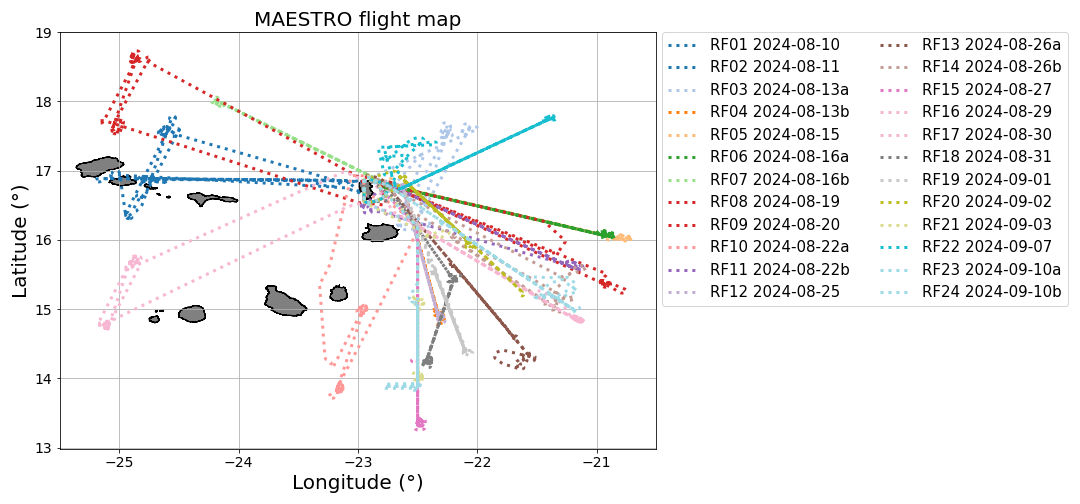
Figure 1 Trajectories of the 24 MAESTRO Research Flights (RF) of the ATR-42. Each flight is named RFXX (MAESTRO nomenclature) or 2024-MM-DDa or b (ORCESTRA nomenclature).

Table 1 Summary of the 24 SAFIRE ATR-42 research flights during the MAESTRO field campaign. Each flight sampled specific cloud types or mesoscale phenomena, with the three sampling strategy types adopted (described in Sect. 2.2). Times of take off and landing (TO-L) are given in local time (UTC−1). Cloud type: ShCu: shallow cumulus; StCu: stratocumulus; AlCu: altocumulus; AlSt: altostratus; Cg: congestus; Phenomena: CP: cold pools; MCS: mesoscale convective system; CL: convergence line. Cloud Cover was obtained from the Météosat Seconde Génération (MSG) satellite in the smallest lat-lon box containing the flight track with the image closest to the middle time of the flight as diagnosed from the algorithm from Derrien and Le Gléau (2005)b in the framework of Eumetsat SAF Nowcasting. Max CT: Maximum Cloud Top, measured with the onboard vertical airborne radar RASTA (Delanoë et al., 2013). Some flights classified as “Case Study” or “Standard” also included coordination elements (see Sect. 2.2 for details).

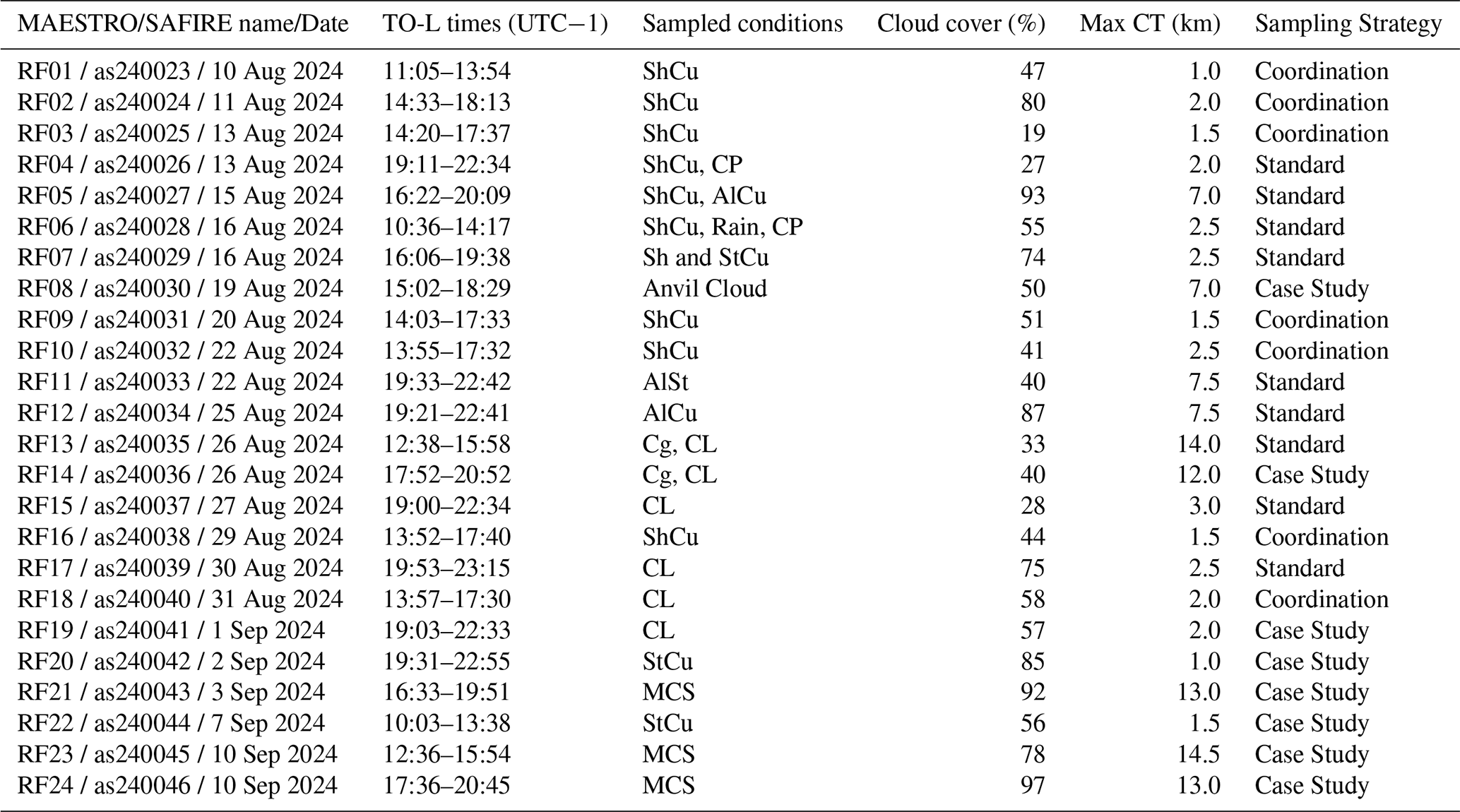
The MAESTRO project primarily aims to test hypotheses regarding the mesoscale organization of shallow and deep convection. Central to this investigation is the role of coherent structures in the boundary layer, such as cold pools and convective plumes, which are believed to significantly influence cloud development and thus contribute to mesoscale convective organization. These elements can affect the statistical properties of the flow (de Szoeke et al., 2017; Zilitinkevich et al., 2006), underscoring the importance of characterizing turbulence to identify their signatures. Table 1 summarizes the cloud types, mesoscale features, cloud cover, and maximum cloud top sampled during each flight. The 24 flights documented diverse phenomena: populations of shallow cumuli (RF01–07, 09, 10, 16), convergence lines (RF13–15, 17–19), cold pools (RF04, 06), isolated convective cells (RF13, 14), and, towards the end of the campaign, mesoscale convective systems (RF21, 23, 24). Mid-tropospheric clouds (StCu and AlCu) were consistently observed and directly sampled with the ATR in-situ instrumentation in five flights (RF5, 11, 12, 20, 22). Overall, cloud cover ranged from 28 % to 100 %, and cloud tops spanned from 1 to more than 14 km, providing the diversity needed to investigate organization processes across scales. A significant shift in synoptic and cloud conditions was documented throughout the campaign, from trade wind regimes with scattered shallow convection in August to deeper conditions in September, with the occurrence of mesoscale convective systems.

2.2 Flight sampling strategies

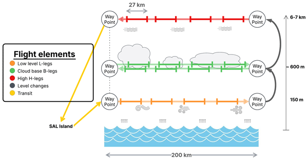
The MAESTRO campaign was dedicated to the gathering of an extensive dataset, representative of various cloud organizations and their surrounding environments, including in situ measurement of subcloud and cloud base levels, as well as cloud geometry with horizontal and vertical remote sensing. To achieve this, a main strategy, denoted in this article as “Standard”, was designed as a series of stacked horizontal legs at predefined flight levels. For nine of the 24 flights, the Standard strategy was implemented for systematic analysis (see Table 1). They consist of sequences of 200 km-long transects denoted as high altitude (H-type), cloud base (B-type), and low altitude (L-type), and performed in this order. A schematic representation of a typical MAESTRO flight plan is given in Fig. 2. The sequence order was sometimes modified, placing the high-altitude transect last. This change improved fuel efficiency by taking advantage of the lighter weight of the aircraft during ascent, enabling higher altitudes to be reached and additional legs to be performed within the spared flight time. S-type (Surface) legs were occasionally flown at about 60 m above the sea surface to document turbulence at the lowest altitude available to the ATR, and could only be flown during day time. However, potential alteration of other instruments due to exposure to sea salt was suspected, in particular for the horizontally pointing Lidar. For this reason, these legs were flown only on a few occasions during the campaign.

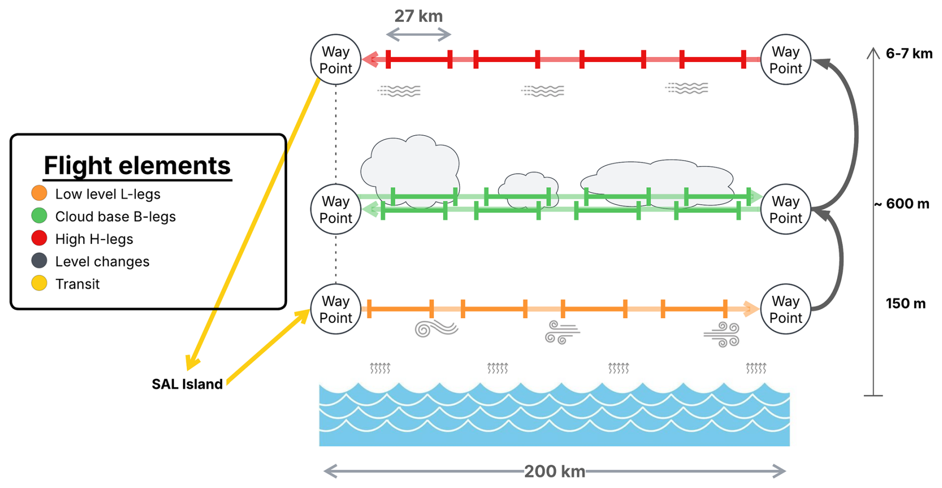
Figure 2 Schematic representation of a flight adopting the Standard strategy. Single arrows symbolize flight elements, such as stabilized legs, transits, or ascents. Line segments bounded by orthogonal end bars symbolize flight segments defined with the segmentation algorithm (see Sect. 3.1.1).

In the event of exceptional convective activity in the vicinity of Sal Island, flight plans were adapted to avoid dangerous areas and prioritize regions of highest scientific interest, this adaptive strategy is designated as “Case Study” (corresponding flights are listed in Table 1). The nomenclature used to name each transect remained similar, allowing the data from all MAESTRO flights to be merged in a single, coherent dataset. Additional segments noted as M- and T-types, were occasionally defined during Case Study flights. These legs enabled upward and downward pointing of remote sensing instrumentation to characterize cloud geometry, as well as to collect in-situ microphysical and thermodynamical measurements in specific regions. Finally, the latter portion of RF22 was dedicated to in-flight calibration maneuvers (described in more details in Appendix A).

In addition to the Standard and Case Study strategies, the campaign also featured flights focused on coordinated measurements with other projects that were part of ORCESTRA. The strategy in all these flights are denoted as “Coordination” in Table 1 if the Standard was not strictly maintained. On seven flights (RF4, RF7, RF11, RF12, RF15, RF16, and RF21), the German DLR HALO aircraft, operating as part of the PERCUSSION campaign, deployed drop-sondes in a circular pattern around the operational area of the ATR-42. This enabled estimates of mesoscale vertical velocity within the region of interest (Bony and Stevens, 2019; George et al., 2021). During RF16 and RF18, cooperation with the King Air aircraft from the CELLO project was performed with both airplanes flying in close formation, either side by side or one above the other. These coordinated operations not only completed the measurements performed on a given day, offering exceptional scientific opportunities, but also made it possible to compare simultaneous remote sensing and in-situ techniques used by the different platforms. Flights RF02, RF03, RF09, RF10, RF16 and RF18 were synchronized and aligned along the satellite track of the newly launched EarthCARE satellite (Wehr et al., 2023) for the calibration and validation of its onboard remote sensing instruments. The flights coordinated with EarthCARE varied only slightly from the Standard flight plan described in Fig. 2, but kept its main elements as much as possible. In particular, to reach Earthcare overpasses, legs were often used to reach the position on time and were then not vertically stacked. During flights RF04, RF05, RF07, RF12, RF15, RF19, and RF20, RADARSAT Constellation Mission (RCM) and/or Sentinel1 satellites acquired Synthetic Aperture Radar (SAR) images collocated with the aircraft track. SAR is sensitive to sea surface roughness, especially centimeter-scale waves . For a complete review of the SAR capabilities see the review of Asiyabi et al. (2023). To take advantage of this, the flight plans were adjusted so S- and L-type legs coincided with the satellite overpasses, providing unique opportunities to investigate sea surface–atmosphere interactions.

This general leg nomenclature is consistent across all MAESTRO datasets, while the specific segmentation described in Sect. 3.1.1 applies to the turbulence dataset presented here. All segment types are summarized as follows:

• H-type (High) transect at mid-tropospheric altitude (6000 $\mathrm{m}\mathrm{a}.\mathrm{s}.\mathrm{l}.$), used for downward-looking remote sensing and in situ measurements of ice clouds and air motion.

• B-type (Base) back-and-forth transects at cloud base, enabling both in situ and horizontally pointing remote sensing observations of the cloud base level, with particular emphasis on cloud–subcloud interactions.

• L-type (Low) transect below the clouds dedicated to in situ measurements within the subcloud layer and upward-looking remote sensing.

• S-type (Surface) flight legs, flown at 60 $\mathrm{m}\mathrm{a}.\mathrm{s}.\mathrm{l}.$, similar in purpose to L-type legs but at lower altitude and for comparisons with SAR radars.

• M-type (mid-level) legs, corresponding to intermediate altitudes between 1 and 4 km.

• T-type (top) legs, corresponding to low-cloud tops, between 1 and 1.5 km.

2.3 Instrumentation for turbulence

The SAFIRE ATR-42 is a research aircraft equipped with a payload of in-situ and remote-sensing instruments. The wind vector is derived from a five-hole nose radome (gust probe), in combination with Pitot-static measurements and an inertial navigation system (INS), following the standard formulation for aircraft wind retrieval (Brown et al., 1983). While some instruments acquire data at rates up to 100 Hz, all variables distributed in the turbulence dataset were resampled to a common 25 Hz frequency, consistent with the EURECA processing choices (Brilouet et al., 2021). At a typical true airspeed of about 100 m s⁻¹, this corresponds to an along-track spacing of about 4 m. We stress that the stored sampling frequency in the original MAESTRO files (25 Hz) should not be confused with the intrinsic temporal response of each instrument: for some sensors (e.g., chilled-mirror hygrometers), the physical response time is much slower than 25 Hz even if the signal is interpolated at that rate. Table 2 summarizes the main characteristics of each in-situ sensor, distinguishing acquisition sampling, nominal response, and the role of each instrument in the final dataset.

Table 2 In-situ instrumentation used for the MAESTRO turbulence dataset. The dataset is distributed at 25 Hz for all variables. The table distinguishes the electronic sampling rate from the native instrument response time. NC: Not communicated.

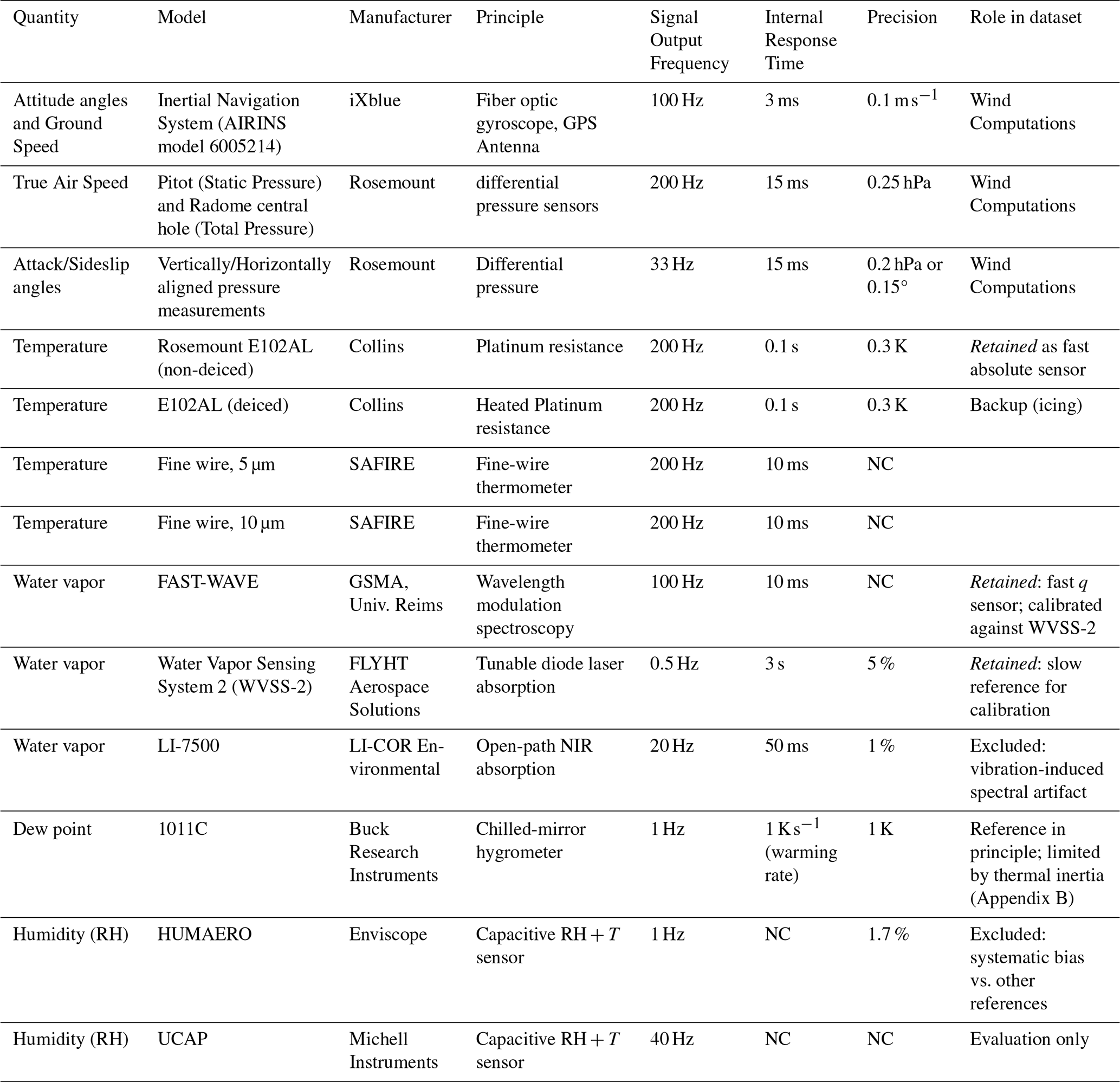
Six hygrometers were operated during the campaign to document water vapor variability across a wide range of conditions and to enable redundancy-based quality assessment. The instruments include: WVSS-2 (laser absorption spectrometer), FAST-WAVE (fast laser absorption spectrometer), an open-path LI-7500 (LI-COR; near-infrared absorption), a 1011C chilled-mirror hygrometer measuring dew point temperature, and two capacitive relative-humidity sensors (HUMAERO and UCAP) associated with their own temperature measurements. Four temperature sensors were also operated: two Rosemount E102AL platinum resistance thermometers (deiced and non-deiced) and two fine-wire probes (5 and 10 µm) designed for fast-response temperature measurements (Ballantyne and Moss, 1977). Additional information on the ATR-42 thermodynamic instrumentation and its general operating principles is provided in Bony et al. (2022).

MAESTRO also served as an opportunity to introduce new instrumentation, one that is particularly relevant to turbulence and cloud studies is the new fast-response hygrometer, FAST-WAVE. This instrument was developed by GSMA (Groupe de Spectrométrie Moléculaire et Atmosphérique) based on the AMULSE technology (Joly et al., 2016), using wavelength modulation spectroscopy. The instrument was housed in a certified antenna mounted on the aircraft fuselage. To validate the integration and acquisition chain, four dedicated test flights were performed in southwestern France in spring 2024. These flights were used to verify the instrument installation, acquisition protocols, and the main data treatment procedures prior to MAESTRO operations.

During the campaign, quick-look time series and spectra were systematically examined after each flight to identify instrumental or processing issues. Three main points relevant for turbulence applications emerged:

1. A non-zero mean vertical wind bias (typically ∼ 0.6 m s⁻¹ when averaged over complete stabilized legs) indicated a calibration issue in the wind retrieval; dedicated in-flight maneuvers enabled us to diagnose and correct constant biases in radome angles, and the correction procedure is described in Appendix A.

2. The LI-7500 exhibited a persistent high frequency spectral artifact peak (above 6 Hz) attributed to potential vibrations of the antenna, which strongly contaminates the high-frequency part of the humidity spectrum; therefore, this instrument is not retained in the final turbulence dataset.

3. A dedicated intercomparison of the three potential reference hygrometers (1011C, WVSS-2, HUMAERO) is provided in Appendix B. While the 1011C chilled mirror provides an absolute measurement in principle, its limited thermal response hampers its ability to track airborne humidity variability in heterogeneous conditions encountered during MAESTRO. WVSS-2 showed the best overall robustness and agreement with the mirror under conditions where the mirror response is not limiting, whereas HUMAERO exhibited varying differences with respect to the 1011C and is therefore not considered as a potential reference.

4. The non-deiced Rosemount E102AL was selected as the temperature sensor for the MAESTRO turbulence dataset. Fine-wire probes, despite their faster intrinsic response time, are highly sensitive to cloud droplet impaction: the less protective housing means that droplet collisions are more likely, rendering the measurement less reliable in cloudy conditions (e.g., Lenschow, 1986). With approximately 38 % of all segments being B-type legs, where cloud droplet encounters are likely, this sensitivity represents a significant limitation for this dataset. The deiced Rosemount sensor avoids droplet impaction through resistive heating, but the heating element introduces a small systematic warm bias that degrades the accuracy of temperature fluctuation measurements in the clear-air conditions that constitute the majority of MAESTRO legs. The non-deiced Rosemount combines a sufficient acquisition frequency and response time for 25 Hz turbulence measurements with robustness across the full range of MAESTRO conditions, and was therefore retained as the reference temperature sensor.

3 Data processing

Reliable turbulence statistics require measurements acquired under quasi-homogeneous flow conditions. The processing workflow described in the current section was designed to optimize this requirement. The wind retrievals received special attention during the MAESTRO campaign and are described in detail in Appendix A. These corrections were applied independently of the processing steps described here and the obtained wind serve as the starting point of the methodology. The MAESTRO turbulence dataset comprises two complementary data products: (1) 25 Hz time series of calibrated wind components, water vapor mixing ratio, and temperature, along with their derived fluctuations, provided both for individual segments and complete flight legs; and (2) segment-scale turbulence statistics including average values, second- and third-order statistical moments, covariances, integral length scales, spectral scaling exponents, and turbulent kinetic energy dissipation rate.

First, all details required to produce the fluctuation time series are described: the filtering of the original time series (Sect. 3.1), the segmentation of the data based on homogeneity of wind fluctuations (Sect. 3.1.1), and the calibration of the humidity signal (Sect. 3.1.2). Second, the restitution of segment-scale statistical properties is described, including computational details for moments and integral length scales (Sect. 3.2), the TKE dissipation rate, and quality assessment metrics: random and systematic errors in statistical moment estimates, and identification of instrumental noise limitations affecting TKE dissipation rate estimates (Sect. 3.3).

3.1 Segmented fluctuation time series

Fluctuations x^′(t) are defined, for any given variable x(t), as:

$$\begin{array}{}\text{(1)}& x\left(t\right)=\stackrel{\mathrm{‾}}{x\left(t\right)}+x^{\prime }\left(t\right)\end{array}$$

where $\stackrel{\mathrm{‾}}{x\left(t\right)}$ is the mean component of x(t). There are multiple ways to extract fluctuations, including removing segment average, detrending, and high-pass filtering. For the MAESTRO turbulence dataset, a high-pass filter is applied with a cutoff frequency of 0.018 Hz, equivalent to filtering mesoscale features larger than approximately 5 km, following the methodology of Brilouet et al. (2021). Because the use of frequency-cutting filters involves arbitrary choices, in particular the numerical method used to approximate the Fourier transform, alternative fluctuations computed with a straightforward linear detrending method are also used later in the dataset to evaluate the impact of the high-pass filtering on statistics.

Once segmentation and pre-processing have been performed (see Sect. 3.1.1 and 3.1.2), the fluctuations at 25 Hz are computed for each segment and for the five variables U_l, V_t, W, θ, and q, where U_l is the horizontal streamwise wind component, V_t the horizontal transverse wind component (obtained by projecting the geographical wind components onto the direction of the segment-averaged wind), W is the vertical air speed, θ the potential temperature, and q the water vapor mixing ratio. In addition, fluctuations of the horizontal wind components are provided in the geographical frame of reference (U_geo and V_geo, the zonal and meridional components, respectively) and in the aircraft frame of reference (U_x and V_y, the longitudinal and transverse components, respectively).

3.1.1 Segmentation of the data

The aircraft legs undergo an automatic segmentation algorithm that creates 4.5 min segments (≈ 27 km) by minimizing the heterogeneity of fluctuations of the three wind components simultaneously. This quantification allows the identification of sufficiently homogeneous segments for reliable statistical moment estimates. The fluctuations of the corrected wind in geographical coordinates are used for the computation of the heterogeneity score.

For a segment with wind perturbations from the three components in the geographical frame of reference $\mathit{\{}{U}_{\text{geo}},V_{\text{geo}},W\mathit{\}}$, the heterogeneity score ℋ is defined as:

$$\begin{array}{}\text{(2)}& \mathcal{H}={\displaystyle \frac{\mathrm{1}}{\mathrm{3}\cdot n}}\sum _{p\in \mathit{\{}{U}_{\text{geo}},V_{\text{geo}},W\mathit{\}}}\sqrt{\sum _{i=\mathrm{1}}^n{\left({\displaystyle \frac{i}{n}}-C_p\left(i\right)\right)}^{\mathrm{2}}}\end{array}$$

where C_p(i) is the normalized cumulative variance at sample index i:

$$\begin{array}{}\text{(3)}& C_p\left(i\right)=\sum _{j=\mathrm{1}}^i{\displaystyle \frac{P_p(j{)}^{\mathrm{2}}}{n{\mathit{\sigma }}_p^{\mathrm{2}}}}\end{array}$$

with P_p(j) the perturbation value at index j for component p, n the total number of data points in the segment, ${\mathit{\sigma }}_p^{\mathrm{2}}$ the variance of p over the segment, and $i/n$ representing an ideal uniform accumulation of variance. ℋ is dimensionless and independent of segment length, so that values remain comparable across segments of different duration or resolutions. The design of this score is based on work done by Bernard-Trottolo (2001). While the original definition only used the vertical wind component, we added both horizontal components to account for heterogeneity in these directions.

ℋ quantifies how unevenly the variance of the wind fluctuations is distributed along a segment. In the rest of the article and in the dataset, ℋ is expressed in %. A homogeneous segment in which variance accumulates steadily throughout will have ℋ≈ 0 %, while a segment containing an abrupt regime change will exhibit a markedly nonlinear cumulative variance profile and therefore a large ℋ. A single dirac step of variance results in the maximum heterogeneity score ℋ = 50 %. The score is invariant to time reversal but sensitive to the shuffling of time steps, which is the desired behavior for detecting regime transitions rather than simply measuring total variance. ℋ has two purposes: (i) to be used in conjunction with the segmentation algorithm to optimize the partitioning of flight legs into segments representing single turbulent regimes, (ii) as a quantitative description of the wind field homogeneity for each sample.

Flight legs are divided into segments of 270 s (4.5 min), using an alternating bi-directional algorithm to minimize overlap and optimize coverage. For each flight leg, the number of fitting segments (n_seg) is determined. The remaining duration R is distributed evenly across all segments to obtain an adjusted segment duration: $\mathrm{\Delta }t=\mathrm{270}\mathrm{s}+R/n_{\text{seg}}$.

Two boundaries are initialized at the start and end points of a given leg: the left boundary $t_{\mathrm{L}}=t_{\text{start}}^{\text{leg}}$ and the right boundary $t_{\mathrm{R}}=t_{\text{end}}^{\text{leg}}<y$. Segments are then extracted alternately from the left and right sides of the remaining leg portion. For even iterations ($n=\mathrm{0},\mathrm{2},\mathrm{4},\mathrm{\dots }$), a search window $[t_{\mathrm{L}},t_{\mathrm{L}}+\mathrm{\Delta }t]$ is defined; the starting position t_min that minimizes ℋ over a 270 s segment is identified, the segment is set to $[t_{\text{min}},t_{\text{min}}+\mathrm{270}\mathrm{s}]$, and the left boundary is updated to $t_{\mathrm{L}}=t_{\text{min}}+\mathrm{270}\mathrm{s}$. For odd iterations ($n=\mathrm{1},\mathrm{3},\mathrm{5},\mathrm{\dots }$), a search window $[t_{\mathrm{R}}-\mathrm{\Delta }t,t_{\mathrm{R}}]$ is defined; t_min is found analogously, the segment spans $[t_{\text{min}},t_{\text{min}}+\mathrm{270}\mathrm{s}]$, and the right boundary is updated to t_R=t_min. After each iteration, R and Δt are computed again. This process continues until all n_seg segments are extracted, working progressively from both ends toward the center. This heuristic balances positioning constraints across all segments while ensuring maximum coverage of each leg.

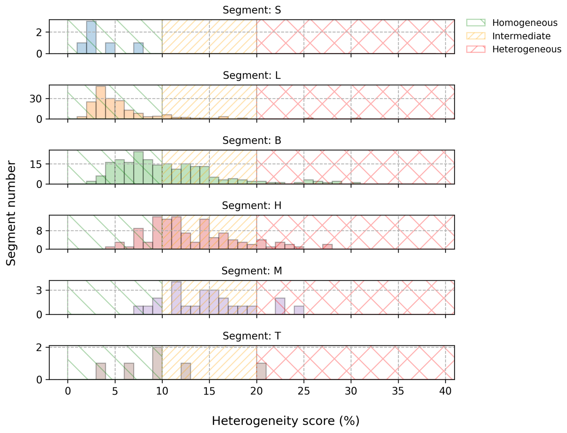
Figure 3 Histograms of ℋ (heterogeneity score) for each segment type. Shaded regions highlight indicative thresholds: scores below 10 % (green) indicate homogeneous segments; scores above 20 % (red) indicate heterogeneous segments; intermediate scores (orange) warrant cautious interpretation.

Figure 3 presents the histograms of ℋ obtained for each segment category throughout the entire MAESTRO campaign. As expected, low-level segments are generally more homogeneous than those collected at higher altitudes. Visual inspection of the time series guided the choice of indicative thresholds to distinguish homogeneous, quasi-homogeneous, and heterogeneous segments; these thresholds are not strict quality gates but serve as guidance for users. Using an upper threshold of 10 % to define homogeneity (green shaded area in Fig. 3), 8 (89 %) S-type and 180 (95 %) L-type segments qualify as homogeneous and are suitable for boundary-layer statistical moment computation. In total, 355 boundary-layer segments (all S-, L-, and B-type segments with ℋ< 10 %) are included in the MAESTRO turbulence dataset as homogeneous.

Segments with ℋ between 10 % and 20 % (orange) can be considered quasi-homogeneous. These likely contain intermittent cloud coverage or alternating air from the boundary layer and free troposphere (particularly for B-types). In the case of L- and S-types, quasi-homogeneous segments typically result from localized atmospheric events such as cold pools, rainfall, or regime transitions. These segments may be used for analysis, but moment estimates are less reliable.

Segments with ℋ exceeding 20 % (red) should not be used for usual turbulence statistics, as such calculations rely on the assumption of quasi-homogeneity. These high scores indicate laminar, non-turbulent, heterogeneous, or intermittent flow, and predominantly occur in high altitude segments classified as H-types. The time-series data can still be used to study gravity waves below the filtered length scales.

3.1.2 Calibration of Humidity Sensors

The accurate measurement of high-frequency humidity fluctuations from an aircraft platform is a longstanding technical challenge. Fast sensors often degrade over time when exposed to cloudy, dusty, or precipitation environments, or may be affected by noise due to imperfect mounting, while slow sensors are relatively stable but lack high-frequency fidelity.

We emphasize that this dataset is optimized for turbulence analysis. The primary objective is to provide accurate turbulence statistics. Consequently, the proper scaling of fluctuation amplitudes and minimal instrumental noise are critical, whereas absolute offsets in mean values are of secondary importance. For example, a 1 g kg⁻¹ bias in mean mixing ratio does not affect the variance $\stackrel{\mathrm{‾}}{q^{\prime \mathrm{2}}}$, but a 10 % error in the calibration slope increases the variance by 21 %. Our approach therefore prioritizes the accurate reproduction of fluctuation amplitudes across scales relevant to turbulence (sub-kilometer to a few meters), rather than absolute mean accuracy. Users requiring accurate absolute values of water vapor mixing ratio, for instance to compute precise relative humidity values, should be aware that the mean value of each calibrated FAST-WAVE signal is that of the WVSS-2 reference, whose absolute accuracy relative to the 1011C is characterized in Appendix B.

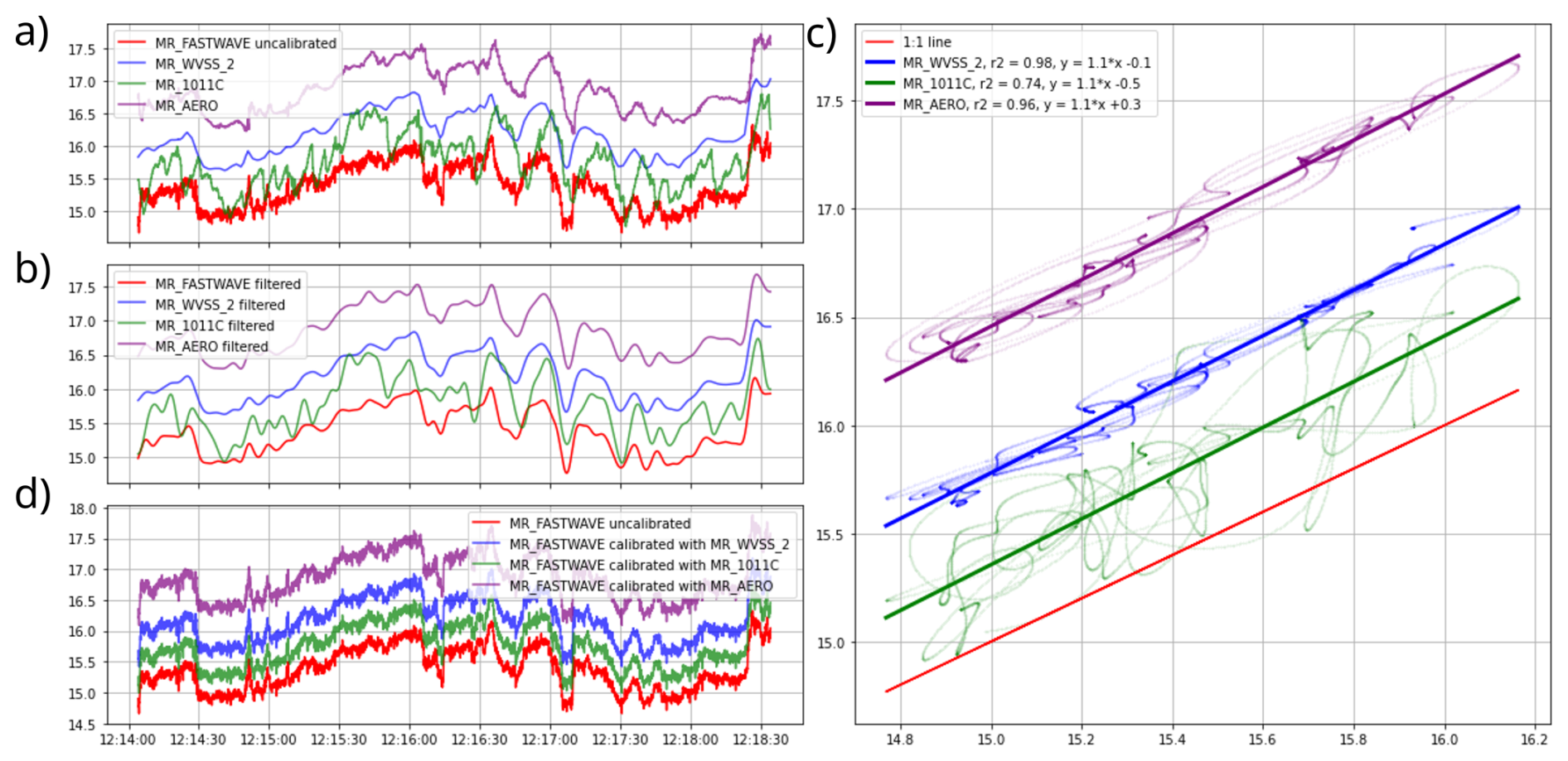
Figure 4 Example application of the calibration methodology for RF06: (a) uncalibrated time series for FAST-WAVE and the three slow sensors (g kg⁻¹); (b) corresponding low-pass filtered time series; (c) linear regression of WVSS-2 (y-axis) against FAST-WAVE; (d) calibrated FAST-WAVE time series.

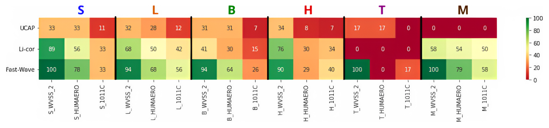
Figure 5 Results of the fast moisture sensor calibration. Percentage of segments with fast-slow sensor low frequency linear regression coefficient R² values above 0.9 for each segment category (heights) and each fast and reference humidity sensor.

It is common practice to calibrate a fast instrument against a slower, more stable reference by maximizing the low-frequency agreement between the two signals, quantified by the coefficient of determination R² after low-pass filtering (Brilouet et al., 2021). This corrects the primary amplitude scaling and instrumental drift. The calibration is performed independently for each segment rather than once per flight or per campaign, for two reasons. First, fast sensors on airborne platforms can experience gradual or abrupt changes in their response characteristics during a flight, due to exposure to clouds, precipitation, salt, and wide ranges of temperature and humidity; a segment-scale calibration accounts for these slow drifts and environment-induced changes. And second, the MAESTRO flight legs sample distinct meteorological regimes at very different altitudes: temperature ranges from approximately +28 °C near the surface to −10 °C at 6000 m, and water vapor mixing ratio spans nearly an order of magnitude between the boundary layer and the mid-troposphere. Capacitive and spectroscopic sensors are known to exhibit environment-dependent sensitivities: the sensitivity of capacitive sensors to relative humidity is a nonlinear function of temperature, while laser absorption spectrometers can be affected by pressure and temperature variations. A segment-scale calibration ensures that the retrieved slope and offset are locally appropriate for the thermodynamic regime actually sampled, rather than imposing a single correction averaged over heterogeneous conditions.

Figure 4 illustrates the procedure for an example segment. For each segment and fast sensor, the fast and reference signals (Fig. 4a) are low-pass filtered with a cutoff at $\mathrm{1}/\mathrm{6}$ Hz (Fig. 4b). The optimal lag between sensors is determined by maximizing their cross-correlation, and a linear regression is fitted to align amplitude and offset (Fig. 4c). Finally, the amplitude and offsets are applied to the original fast sensor signal to obtain calibrated time-series (Fig. 4d). Segment-sensor pairs with R²>0.9 indicate satisfactory agreement on large-scale structure.

We acknowledge that this approach has a limitation in segments where the thermodynamic field is nearly horizontally homogeneous,for instance in weakly turbulent or laminar layers. In corresponding segments, the low-frequency variability available for the regression is small, the fitted slope is uncertain, and the calibration is less constrained. For these cases, the R² criterion (R²>0.9) indicates where the low-frequency variability is potentially insufficient to produce a reliable regression. This is consistent with the general observation that weakly turbulent H-type segments, where horizontal homogeneity is expected, also show the lowest R² values in the calibration results.

Although technical limitations of the 1011C and chilled-mirror hygrometer and the HUMAERO capacitive sensor have been highlighted in Appendix B and reported in the instrumentation Sect. 2.3, we included them in the calibration procedure to further confirm our choice. The outcome of the calibrations of fast humidity sensors is presented in Fig. 5, categorized by segment type and each possible reference-fast sensor couplings. FAST-WAVE demonstrates the best agreement across all segment types and for each reference sensors, with only rare exceptions in a few T and H segments. Among the reference sensors, WVSS-2 consistently shows the best agreement across all segment types and fast sensors, except for the T-segments, where UCAP aligns better with HUMAERO than WVSS-2. Overall, the results demonstrate poor compatibility between UCAP and any reference sensor. FAST-WAVE and WVSS-2 are the most reliable combination for humidity calibration, achieving effective performance across 94 % of the segments. This highlights their robust compatibility and suitability for diverse conditions. On the basis of these results and to provide a consistent dataset, FAST-WAVE fluctuations, calibrated against the WVSS-2 are selected as the base signal for humidity fluctuations and computations of turbulent statistics.

3.2 Statistical description of segments

In the dataset, only horizontal components in the wind-aligned frame of reference (U_l and V_t) are used for the statistical description of individual segments. However, in the files, the suffixes are not repeated to maintain clarity. By projecting the wind onto the direction of the segment-averaged wind, the variance and covariance estimates represent fluctuations relative to the local flow, rather than with respect to fixed geographic or aircraft axes. This approach ensures that the statistics are physically interpretable and consistent across segments with differing sampling or wind directions.

3.2.1 Second- and third-order statistical moments

The 25 Hz fluctuations are used to compute segment-scale statistics. To compute these estimates, the only horizontal wind component used are those in the wind-oriented frame of reference. Second-order moments (variance for every of the five variables: U_l, V_t, W, θ, q and covariance of each possible variable couple) provide information about the energy contained in the fluctuations. In the moment dataset, variances are identified by the VAR_ prefix, and covariances by the COVAR_ prefix. For any two variables x and y and a segment of duration ΔT, the eddy-correlation method gives:

$$\begin{array}{}\text{(4)}& \stackrel{\mathrm{‾}}{x^{\prime }{y}^{\prime }}={\displaystyle \frac{\mathrm{1}}{\mathrm{\Delta }T}}\underset{\mathrm{0}}{\overset{\mathrm{\Delta }T}{\int }}{x}^{\prime }\left(t\right)y^{\prime }\left(t\right)\mathrm{d}t\end{array}$$

where the overbar denotes a temporal average over the segment. The variance of a single variable x is the special case $\stackrel{\mathrm{‾}}{x^{\prime \mathrm{2}}}$.

Among covariance estimates, those of direct physical relevance include the vertical turbulent fluxes of momentum ($\stackrel{\mathrm{‾}}{U^{\prime }{W}^{\prime }}$, $\stackrel{\mathrm{‾}}{V^{\prime }{W}^{\prime }}$), heat ($\stackrel{\mathrm{‾}}{W^{\prime }{\mathit{\theta }}^{\prime }}$), and moisture ($\stackrel{\mathrm{‾}}{W^{\prime }{q}^{\prime }}$). The momentum fluxes quantify the vertical transport of horizontal momentum and drive the wind shear structure of the boundary layer. $\stackrel{\mathrm{‾}}{W^{\prime }{\mathit{\theta }}^{\prime }}$ controls buoyancy-driven convection and is a key driver of boundary-layer growth. $\stackrel{\mathrm{‾}}{W^{\prime }{q}^{\prime }}$ governs the supply of moisture to the cloud layer, important to boundary layer convection and associated cloud formation. $\stackrel{\mathrm{‾}}{U^{\prime }{V}^{\prime }}$ quantifies horizontal shear production of TKE. And finally, the temperature-humidity covariance ($\stackrel{\mathrm{‾}}{{\mathit{\theta }}^{\prime }{q}^{\prime }}$) is related to buoyancy effects in moist air and can be related to the partitioning between heat and moisture contributions to the buoyancy flux.

Turbulent kinetic energy per unit mass (TKE) is defined as:

$$\begin{array}{}\text{(5)}& \text{TKE}={\displaystyle \frac{\mathrm{1}}{\mathrm{2}}}\left(\stackrel{\mathrm{‾}}{U^{\prime \mathrm{2}}}+\stackrel{\mathrm{‾}}{V^{\prime \mathrm{2}}}+\stackrel{\mathrm{‾}}{W^{\prime \mathrm{2}}}\right)\end{array}$$

and is provided in the dataset under the variable name TKE. It gives a global measure of the intensity of turbulent motions and is a key input for turbulence parameterization schemes in numerical models.

Third-order moments and skewness are also computed for the five variables. The third-order moment $\stackrel{\mathrm{‾}}{x^{\prime \mathrm{3}}}$ and the normalized skewness $\text{Sk}\left(x^{\prime }\right)=\stackrel{\mathrm{‾}}{x^{\prime \mathrm{3}}}/(\stackrel{\mathrm{‾}}{x^{\prime \mathrm{2}}}{)}^{\mathrm{3}/\mathrm{2}}$ characterize the asymmetry of the probability distribution of fluctuations. Non-zero skewness of vertical velocity (Sk(W^′)) can be indicative, for instance, of meteorological elements such as narrow updrafts and broad downdrafts, typical of convective boundary layers (Lenschow, 1986). In the dataset, third-order moments are identified by the M3_ prefix, and skewness by the SKEW_ prefix. All second- and third-order moments, as well as skewness values, are provided both from high-pass filtered fluctuations and from detrended fluctuations (identified by the _DET suffix), to allow users to assess the sensitivity of the statistics to the choice of mean-field removal method.

3.2.2 Integral length scale and inertial-range spectral slope

The integral length scale L_x is defined as the distance over which fluctuations of a variable x remain significantly correlated. It is obtained as the integral of the autocorrelation function up to its first zero crossing (Lenschow et al., 1994) (Fig. 6a and b):

$$\begin{array}{}\text{(6)}& L_x=U_{\mathrm{a}}\underset{\mathrm{0}}{\overset{{\mathit{\tau }}_{\mathrm{0}}}{\int }}{R}_{xx}\left(\mathit{\tau }\right)\mathrm{d}\mathit{\tau }\end{array}$$

where R_xx(τ) is the normalized autocorrelation function, τ the time lag, τ₀ the time lag corresponding to the first zero crossing of R_xx, and U_a is the true airspeed used to convert from time lag to length. The integral length scale gives a characteristic size of the largest energy-containing eddies and indicates the average spatial extent over which turbulent structures persist (Fig. 6c). It is a key parameter for characterizing the dominant turbulent structures in the boundary layer, and for quantifying sampling adequacy through the random error estimates (Sect. 3.3.1).

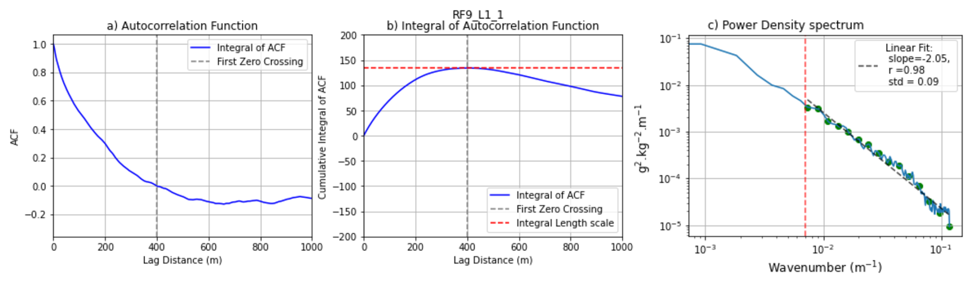
Figure 6 Example autocorrelation function (a), its integral (b), and the derived power spectrum (c) for the water vapor mixing ratio measured with FAST-WAVE for segment L1-1 of RF09. In (c), “r” is the determination coefficient, and “std” the root mean square errors between the spectrum and the fitted curve in log scale, taken for equally spaced points in log scale, represented in green in (c).

Integral length scales are computed for each of the five variables (L_U, L_V, L_W, L_θ, L_q) as well as for all ten cross-correlation pairs (e.g. L_Wθ, L_Wq, etc.), and are provided in the segment statistics files. In particular, L_W is used as input to the TKE dissipation rate computation described below. For each variable, the inertial-range spectral slope is also extracted. The power spectral density is computed using a Fast Fourier Transform on the fluctuation time series, and a linear regression in log-log space is performed over the inertial subrange, defined from the wavenumber corresponding to the integral length scale $k_{\text{IL}}=\mathrm{2}\mathit{\pi }/L_x$ up to the Nyquist wavenumber (as illustrated in Fig. 6c).

3.2.3 Turbulent kinetic energy dissipation rate

The TKE dissipation rate ε measures the rate at which turbulent kinetic energy is converted into heat through viscous effects at small scales. In the case of aircraft measurements with a spatial resolution of 4 m, the dissipation range lies beyond the scope of direct observations.

Following standard practice for aircraft turbulence measurements (Lenschow, 1986), ε is computed from the vertical wind component W, which is less affected by mesoscale horizontal variability and more reliably captures isotropic fluctuations in the inertial subrange. Assuming locally homogeneous and isotropic flow (Kolmogorov, 1991), the one-dimensional power spectrum of W in the inertial subrange takes the form:

$$\begin{array}{}\text{(7)}& S_W\left(k\right)={\displaystyle \frac{\mathrm{4}}{\mathrm{3}}}\mathit{\alpha }{\mathit{\epsilon }}^{\mathrm{2}/\mathrm{3}}{k}^{-\mathrm{5}/\mathrm{3}}\end{array}$$

where α=0.52 is the Kolmogorov constant for the vertical-velocity spectrum, taking the values obtained by Sreenivasan (1995) and Wyngaard and Coté (1971). This expression assumes that the spectral slope in the inertial subrange is exactly $-\mathrm{5}/\mathrm{3}$. Using the formula of Lambert and Durand (1998), and defining the inertial subrange from the integral length scale wavenumber k_IL up to an upper bound k_max (discussed below), ε is computed as:

$$\begin{array}{}\text{(8)}& \mathit{\epsilon }={\mathit{\sigma }}_f^{\mathrm{3}}{\left[\mathrm{2}\mathit{\alpha }\left(k_{\text{IL}}^{-\mathrm{2}/\mathrm{3}}-k_{\text{max}}^{-\mathrm{2}/\mathrm{3}}\right)\right]}^{-\mathrm{3}/\mathrm{2}}\end{array}$$

where ${\mathit{\sigma }}_f=\sqrt{{\int }_{k_{\text{IL}}}^{k_{\text{max}}}{S}_W\left(k\right)\mathrm{d}k}$ is computed by integrating the W power spectral density over the inertial subrange.

In the absence of instrumental noise, k_max is set to the Nyquist wavenumber (12.5 Hz ≈ 0.8 rad m⁻¹ at 100 m s⁻¹). However, the accuracy of ε estimates is fundamentally limited by instrumental noise at high wavenumbers, which becomes relevant in low-turbulence conditions where W fluctuation amplitudes are small. Following Muschinski et al. (2001), we assessed the spectral noise floor of the vertical wind measurements. Analysis of S_W(k) across all segments revealed that instrumental noise begins to influence the spectrum when spectral density values fall below approximately 2 × 10⁻⁶ m¹ s⁻². Such contamination can be observed exclusively in some H-type segments at mid-tropospheric altitudes; for all boundary-layer segment types (S, L, B), no spectral contamination by instrumental noise was detected.

To prevent noise from biasing ε estimates, k_max is therefore defined as the minimum of the Nyquist wavenumber and the first wavenumber at which S_W(k) falls below 1 × 10⁻⁵ m¹ s⁻², which is a conservative threshold approximately five times the observed noise floor. In practice, this truncation affects primarily weak-variance H-type segments; boundary-layer segments retain their full inertial subrange.

Let us consider the uncertainty of ε associated with the assumption $S_W\left(k\right)\propto k^{-\mathrm{5}/\mathrm{3}}$ throughout the integration range in Eq. (7). When the observed spectral slope deviates from $-\mathrm{5}/\mathrm{3}$, the integrated vertical wind variance ${\mathit{\sigma }}_f^{\mathrm{2}}$ changes, introducing a bias in the retrieved ε. To quantify this sensitivity, we numerically evaluated Eq. (8) for a spectrum of the form $S_W\left(k\right)=\frac{\mathrm{4}}{\mathrm{3}}\mathit{\alpha }{\mathit{\epsilon }}^{\mathrm{2}/\mathrm{3}}{k}^s$, where the slope $s=-\mathrm{5}/\mathrm{3}+\mathit{\delta }$ is varied. ε is kept constant, and the retrieval of ε uses Eq. (8), still assuming the $-\mathrm{5}/\mathrm{3}$ slope and meaning the error associated with a slope deviation is not only sensitive on δ, but also slightly on the integration range as σ_f is still evaluated on the s-scaled spectrum.

For parameters representative of L-type segments (integral length scale L_W = 50 m corresponding to k_IL≈ 0.13 rad m⁻¹, k_max equal to the Nyquist wavenumber ≈ 0.8 rad m⁻¹), a slope deviation of $\mathit{\delta }=+\mathrm{0.1}$ (i.e., an observed slope of −1.57 instead of $-\mathrm{5}/\mathrm{3}$) leads to an underestimation of ε by approximately −18 %, while a deviation of $\mathit{\delta }=-\mathrm{0.1}$ (slope of −1.77) causes an overestimation of approximately +23 %. For parameters representative of H-type segments (integral length scale L_W = 200 m corresponding to k_IL≈ 0.03 rad m⁻¹, k_max equal to the Nyquist wavenumber ≈ 0.8 rad m⁻¹), a slope deviation of $\mathit{\delta }=+\mathrm{0.1}$ (i.e., an observed slope of −1.57 instead of $-\mathrm{5}/\mathrm{3}$) leads to an underestimation of ε by approximately −30 %, while a deviation of δ = −0.1 (slope of −1.77) causes an overestimation of approximately +43 %. Segments where the parameter corresponding to the extracted spectral slope of the vertical wind (Slope_W) deviates substantially from $-\mathrm{5}/\mathrm{3}$ should be treated with caution when interpreting absolute values of ε.

Unlike fixed-scale approaches (e.g. Muschinski et al., 2001), which use a fixed wavelength range, our formulation dynamically adapts the spectral range to the integral length scale of each segment. In weakly turbulent H-type segments, L_W typically reaches 200 m, so the integration extends over a substantial wavenumber range before encountering the noise floor, yielding meaningful ε estimates even in relatively quiescent conditions. In highly turbulent boundary-layer segments, the integral length scale is tens of meters and the full inertial subrange up to the Nyquist limit is retained.

Similar methodological choices have been made in comparable aircraft studies (Brilouet et al., 2021; Shaw and Businger, 1985; Wacławczyk et al., 2020, 2017; Jen-La Plante et al., 2016; Malinowski et al., 2013), enabling direct comparison with prior field campaigns. Users requiring precise absolute values of ε at low turbulence levels are advised to consult the corresponding spectral slopes (Slope_W) and integral length scale (L_W) included in the segment statistics files as additional quality indicators that can be used to test the validity of the assumptions used.

3.3 Quality assessment

It is important to note that the accuracy of turbulence statistics is inherently dependent on the intensity of turbulence itself. In weakly turbulent, intermittent, or near-laminar conditions, predominantly for some tropospheric segments (B-, H-, T-, and M-types), the small magnitude of fluctuations may approach instrumental detection limits, making statistical estimation more uncertain. These conditions are identifiable through multiple quality indicators: low variance values, relatively high random errors, spectral slopes near or above −1 signalling possible noise contamination, and high heterogeneity scores ℋ, which often indicate transitions between turbulent and laminar regimes or intermittent turbulence. Users should interpret moments from weakly turbulent segments with caution.

3.3.1 Random error

Beyond instrumental limitations, the reliability of statistical moment estimates depends on sampling conditions. Following Lenschow et al. (1994), the random error ϵ_r is inherent to the finite segment length relative to the integral length scale. For any two variables x and y:

$$\begin{array}{}\text{(9)}& {\mathit{ϵ}}_{\mathrm{r}}=\sqrt{{\displaystyle \frac{\mathrm{2}{L}_{xy}}{L}}}\sqrt{\mathrm{1}+{\displaystyle \frac{\mathrm{1}}{r_{xy}^{\mathrm{2}}}}}\end{array}$$

where L_xy is the integral length scale of $x^{\prime }{y}^{\prime }$, L the segment length, and r_xy the correlation coefficient between x and y. For the variance of a single variable x:

$$\begin{array}{}\text{(10)}& {\mathit{ϵ}}_{\mathrm{r}}=\mathrm{2}\sqrt{{\displaystyle \frac{L_x}{L}}}\end{array}$$

In both cases, reliable estimates require L≫L_xy (or L≫L_x).

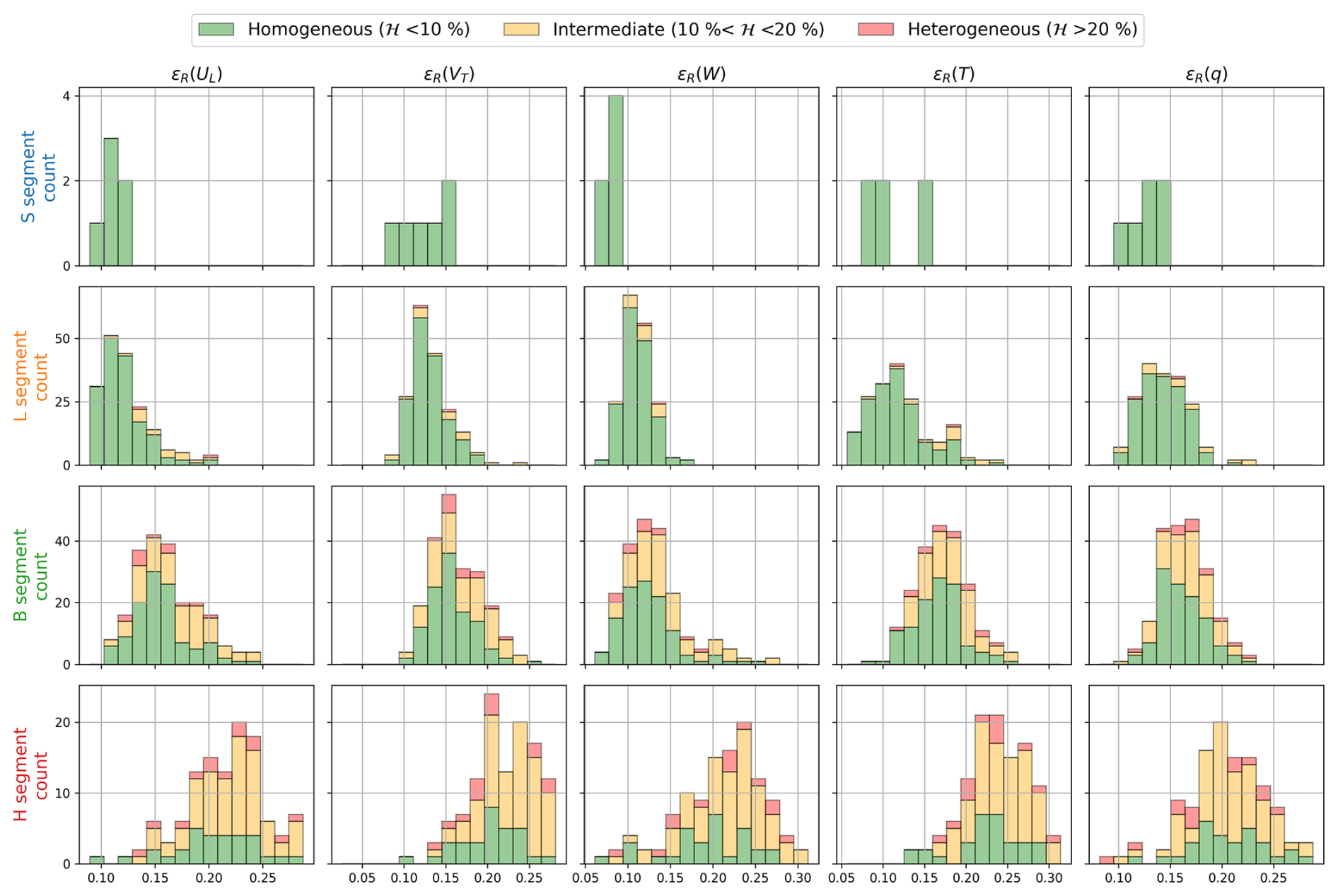
Figure 7 Histograms of random errors for the variances of all five variables, for each segment type. Colors indicate the heterogeneity class of each segment.

Figure 7 shows the histograms of ϵ_r for the whole campaign and for S-, L-, B-, and H-type segments. For the three boundary-layer categories (S, L, B), most segments show variance random errors below 20 %, with positively skewed distributions. For the H category, the only segment type with a statistically large sample size outside the boundary layer, the distributions are negatively skewed and centered around 20 %–30 %, consistent with the larger integral length scales expected in the free atmosphere. The heterogeneity score coloring confirms overall agreement between ℋ and ϵ_r: homogeneous segments (green) exhibit low random errors, while the high ϵ_r values in H-type segments with elevated ℋ (red, orange) reflect the mismatch between the fixed segment length and the large integral scales of laminar or intermittent flow.

3.3.2 Systematic error

The definition of the mean field directly influences the magnitude of the fluctuations, and the choice of a 5 km high-pass cutoff removes variance at scales larger than 5 km. To quantify this filtering effect, which is called systematic error (ϵ_S) the covariance of the high-pass-filtered series (F_fil) is compared to that of the detrended series (F_det):

$$\begin{array}{}\text{(11)}& {\mathit{ϵ}}_{\mathrm{f}}={\displaystyle \frac{F_{\text{det}}-F_{\text{fil}}}{F_{\text{det}}}}\end{array}$$

This quantity is computed for every second-order moment (variances and covariances) and provided in the dataset. It is not a systematic error in the classical sense (cf. Lenschow et al., 1994, who define systematic error as the inherent bias from approximating ensemble means with finite-sample temporal averages). Instead, it quantifies the variance suppressed by the choice of cutoff scale.

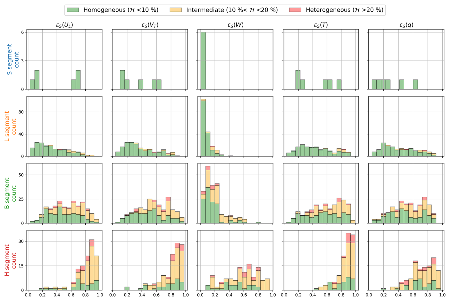
Figure 8 Histograms of the filtering-induced variance loss for all five variables, for each segment type.

Figure 8 shows the histograms of ϵ_f for all five variables and each segment type. For the boundary-layer types (S, L, B), the distribution of ϵ_f for vertical wind variance is much narrower and confined entirely below 25 %, reflecting the small contribution of large scales to the vertical wind in the mixed layer. For the other four variables, substantially more variance is removed by the 5 km filter, revealing the relatively stronger mesoscale influence on thermodynamic fields. The heterogeneity score coloring shows a strong link between ℋ and ϵ_f: non-linear trends in the large-scale component, associated with regime transitions or mesoscale structures, produce both high heterogeneity scores and large filtering effects.

4 Dataset summary

The nomenclature for the dataset file names and their content is given in Table 3. The dataset is divided by flight, legs and segments as explained below:

1. SEGMENT_STATISTICS (one file per flight). The statistical moments and associated errors, along with segment-averaged values for each thermodynamic variable, are provided for each segment. Additionally, the starting, and ending coordinates, mean true heading, true airspeed, and ground speed for a given segment are included.

2. SEGMENT_TIMESERIES (one file per segment). For each segment, one file is generated that includes the 25 Hz geographical coordinates, the corrected horizontal wind components in the geographic, stream-wise, and plane's frame of reference, the corrected vertical wind component, the calibrated water vapor mixing ratio, and potential temperature. In addition, fluctuations of the horizontal stream-wise wind components, vertical wind component, water vapor mixing ratio, and potential temperature are provided for high-pass filtered data.

3. LEG_TIMESERIES (one file per flight elements). For each leg, or specific flight element (D, A, and V, meaning decent, ascent, and Velocity Azimuth Display, respectively) one file is generated with a 25 Hz temporal resolution, without constraints on homogeneity. The variables within these files include 3D-Wind in the three coordinate systems (streamwise, aircraft frame of reference, and geographical), water vapor mixing ratio, and potential temperature. The purpose of this approach is to provide a suitable dataset for users wanting to study the variability along entire legs from turbulence to mesoscale, develop specific analyses, revise segmentation, identify specific meteorological patterns or events in the time series, or use ascents and descents to obtain vertical atmospheric profiles.

Table 3 MAESTRO turbulence dataset structure and variables. File nomenclature: file names begin with MAESTRO_ORCESTRA_ATR_TURBULENCE_^∗ YYYYMMDD = flight date (e.g., 20240815), NN = campaign flight number (e.g., 09), ZZ = SAFIRE flight identifier, X = leg identifier, i = segment identifier (e.g., L2_1), V = file version. Unless stated otherwise, statistics were computed using high-pass filtered fluctuations and using the wind-oriented frame of reference (U_l and V_t). Quantities obtained form detrended series are annotated with the _DET suffix. Random and systematic errors are available for each covariance and variance variable.

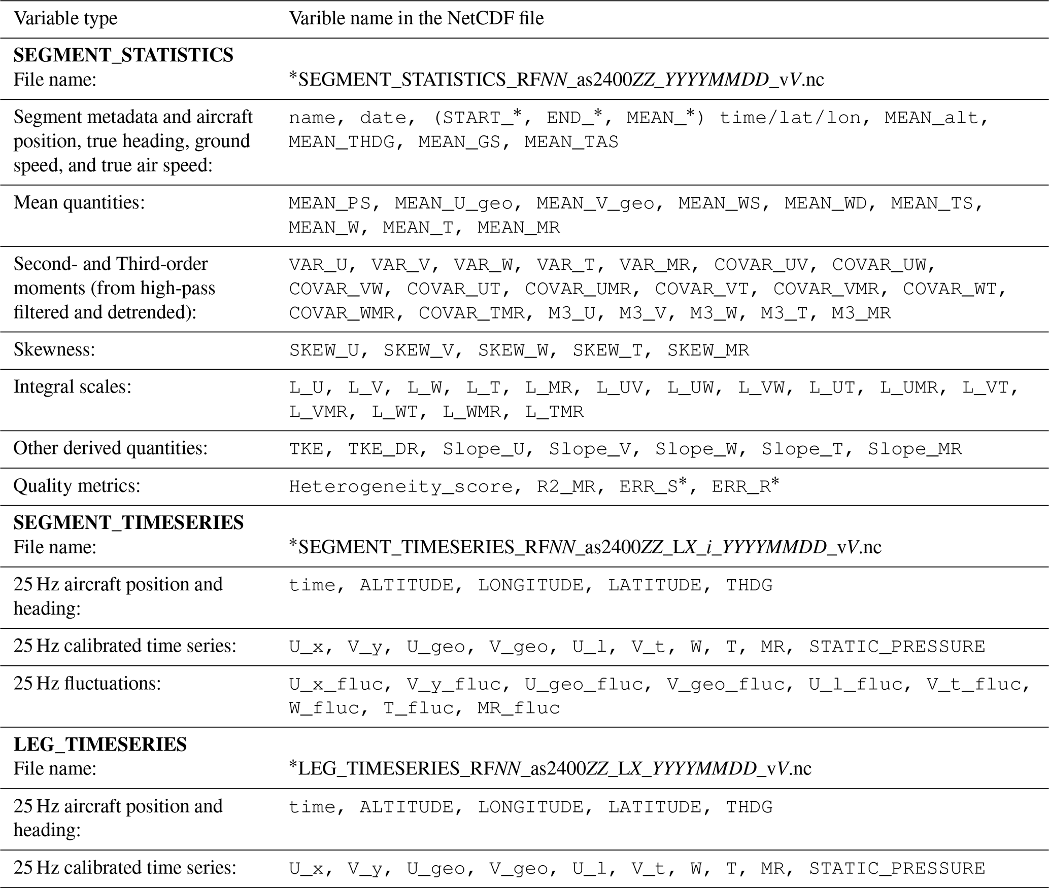
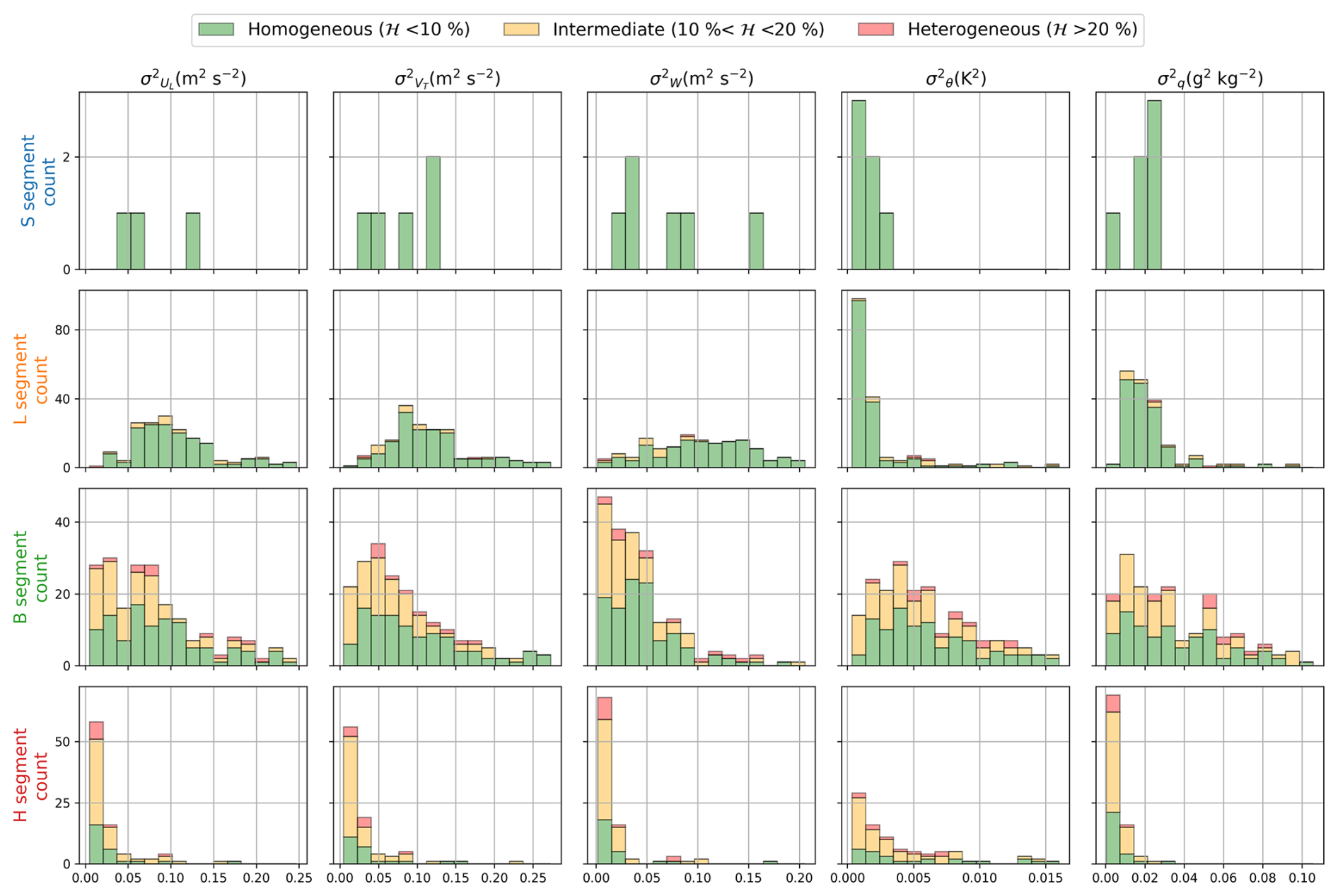
Figure 9 Histograms of computed variance for each segment category and the 5 high-pass filtered variables.

As a preview of the turbulence measured during the MAESTRO campaign, Fig. 9 presents histograms of the variances, computed from the high-pass filtered series for each segment category. The instruments used to compute these moments are the one selected for the dataset, after corrections and calibrations, as described in Sect. 3. For the three wind components in the streamwise frame of reference, the variance is usually higher within the boundary layer, in particular in L-segments. These high variance values indicate more turbulent flow near the ocean surface, which is characteristic of the atmospheric boundary layer.

For temperature and water vapor mixing ratio, cloud-base segments (B-type) are associated with the highest variance values. B-type legs are horizontal transects flown at cloud-base level. Two possible contributing factors can be identified: (1) the aircraft may alternately encounter clear air and cloud interior during partially cloudy segments, generating along-track horizontal gradients in both T and q due to the contrasting thermodynamic properties of these two environments, and (2) even in segments that are fully within the clouds, the cloud interior itself is a region of strong thermodynamic heterogeneity, where active condensation, evaporation, and mixing processes produce large local fluctuations in temperature and humidity.

Figure 10 Histograms of TKE dissipation rates for the turbulence dataset.

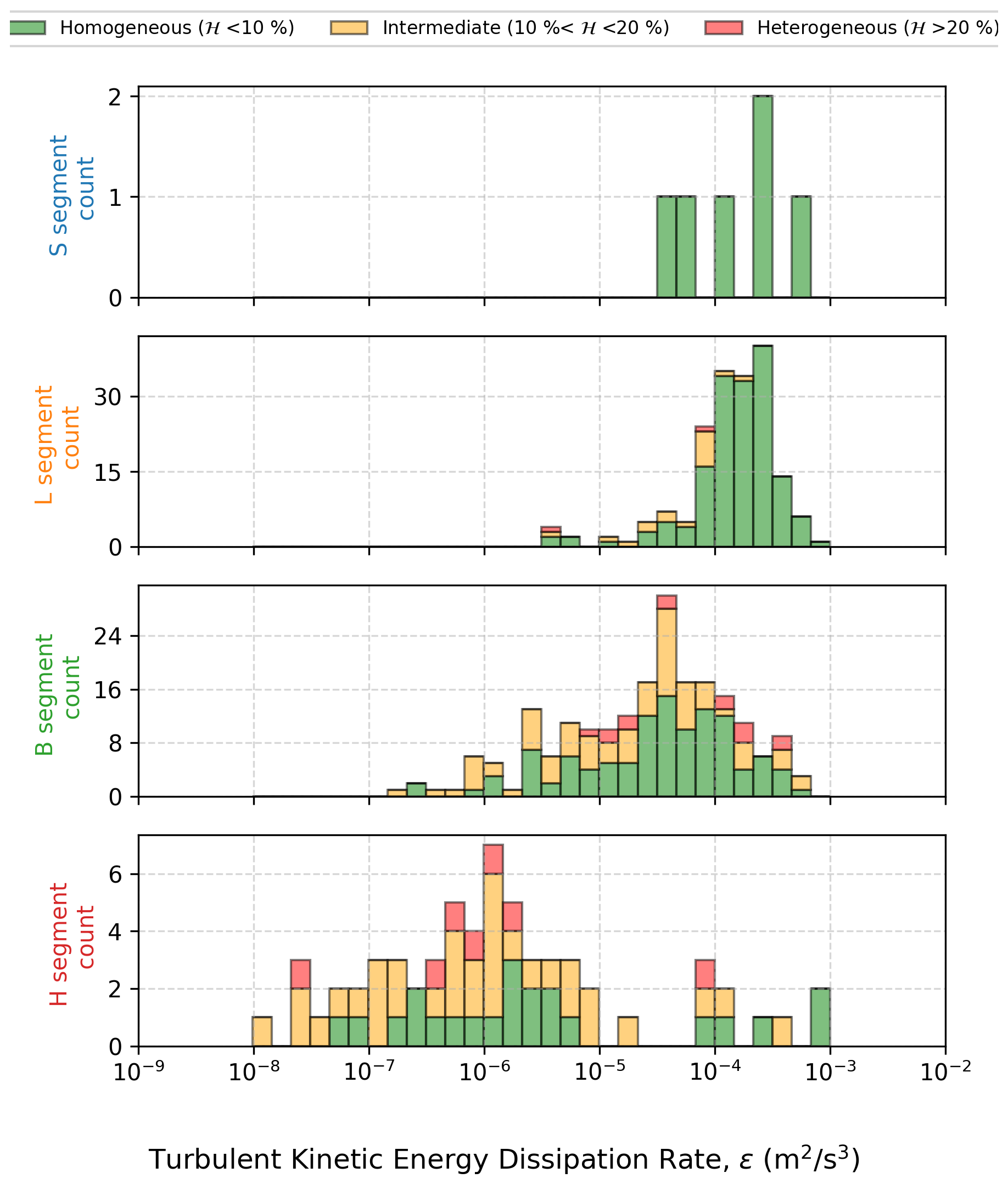
Figure 10 shows the TKE dissipation rate measured during MAESTRO. The general trend is an increase towards the sea surface (segments L and S) whose roughness contributes to turbulence. The obtained values for mixed layer segments (L and S types) are in-line with the one that can be found in the literature (for example in Lambert and Durand, 1998) ranging between 10⁻⁴ and 10⁻³ m² s⁻³. For higher altitudes, the values decrease substantially as flow regimes become more laminar and less energetic.

5 Code and data availability

Code is available on request to the corresponding authors. The turbulence dataset is available at https://doi.org/10.25326/812#v7.0 (Jaffeux and Lothon, 2025). The raw datasets used for this study are available on the AERIS website (https://doi.org/10.25326/738, Bony, 2024a; and https://doi.org/10.25326/744, Bony, 2024b).

6 Conclusions

The article presents the MAESTRO turbulence dataset, based on the in-situ wind, temperature, and moisture measurements from the instrumented ATR-42 from SAFIRE during the MAESTRO field campaign. It presented the sampling strategy and processing details. The quality of the variables of the dataset has been assessed, including the computation of systematic and random errors. On the one hand, the moment dataset can be used to perform process studies or model validation, as it summarizes the turbulence and mean data effectively in few key metrics that can be easily compared across segment types or flights. On the other hand, leg-scale time series dataset can be used to identify larger scales spatial variations that were cut off by the filtering. Calibrated time series at the leg scale enable finer analysis or reprocessing of the data to perform specific analyses with various methods such as wavelet analysis. Providing both types of data ensures the best and broadest utilization of the turbulence data collected during the MAESTRO field campaign.

With the data quality analysis, a few comments and recommendations for users of this dataset can be formulated. Nan values can be present in the moment and legs time series files. In the moment files, inertial slopes may contain NaN values if the inertial range is too small to be able to derive a reliable slope estimate or if the regression coefficient is below 0.9. The TKE dissipation rate ε can also take NaN values if the inertial range of the vertical wind component spectrum is too small. In the leg time series, NaN values are associated with INS malfunctions affecting altitude, latitude, longitude, static pressure, true heading, and all wind components. NaN values can be found in 12 of the 269 leg time series files. In the segment time series, NaN values are avoided through the use of the segmentation algorithm. For turbulence statistics, segments with a heterogeneity score below 10 % can be considered homogeneous and should be prioritized. Additionally, the treatment of FAST-WAVE data will be improved to better resolve frequencies higher than 25 Hz. A dedicated 100 Hz dataset will be released on the AERIS website following this publication.

While being a valuable resource for the broad atmospheric research community, the present dataset was primarily collected to address the MAESTRO research questions. The data presented in this article will be used to examine the relationships between turbulence characteristics within the marine boundary layer and the organization of convection in the tropics. As one of several MAESTRO and ORCESTRA datasets, it will be integrated with other observations to conduct analyses targeted at these research questions. Other datasets include sounding near Sal airport, airborne remote sensing instruments, satellite observations, and in-situ microphysics. Among the satellite products that were gathered during the campaign, SAR images are particularly promising. They document the centimeter-scale waves at the surface of the ocean (Atlas, 1994), thus they are relevant to the study of turbulence in the marine boundary layer and sea-air-cloud interactions (Brilouet et al., 2023; Kudryavtsev et al., 2005). Seven flights of the campaign were planned with respect to these acquisitions so that the plane was concomitantly performing a full leg at 150 m above the surface of the ocean. Exploring these data could lead to better interpretations of SAR images and plane turbulence data, and ultimately improve the current understanding of air-sea interactions within the tropical convective environment. This represents one of the direct research avenues for this dataset and a potential building block for further analyses, hopefully advancing the more fundamental questions that motivated MAESTRO and ORCESTRA.

Appendix A: Wind Corrections

The air velocity components are obtained by subtracting the ground velocity of the aircraft, measured by the INS, from the air velocity with respect to the aircraft, deduced from differential pressures measured by the five-hole nose radome and a Pitot tube. While gust probes are calibrated to mitigate flow disturbance effects, multiple sources of error can affect wind retrieval, including uncertainties in instrument alignment and performance. The full wind component equations in geographical coordinate are the following:

$$\begin{array}{}\text{(A1)}& {\displaystyle }\begin{array}{rl}{U}_{\text{geo}}=& -U_{\mathrm{a}}\cdot D^{-\mathrm{1}}[\sin \mathit{\psi }\cos \mathit{\theta }+\tan \mathit{\beta }(\cos \mathit{\psi }\cos \mathit{\varphi }\\ & +\sin \mathit{\psi }\sin \mathit{\theta }\sin \mathit{\varphi })+\tan \mathit{\alpha }(\sin \mathit{\psi }\sin \mathit{\theta }\cos \mathit{\varphi }\\ & -\cos \mathit{\psi }\sin \mathit{\varphi }\left)\right]+U_p-L(\dot{\mathit{\theta }}\sin \mathit{\theta }\sin \mathit{\psi }\\ & -\dot{\mathit{\psi }}\cos \mathit{\psi }\sin \mathit{\theta })\end{array}\text{(A2)}& {\displaystyle }\begin{array}{rl}{V}_{\text{geo}}=& -U_{\mathrm{a}}\cdot D^{-\mathrm{1}}[\cos \mathit{\psi }\cos \mathit{\theta }-\tan \mathit{\beta }(\sin \mathit{\psi }\cos \mathit{\varphi }\\ & -\cos \mathit{\psi }\sin \mathit{\theta }\sin \mathit{\varphi })+\tan \mathit{\alpha }(\cos \mathit{\psi }\sin \mathit{\theta }\cos \mathit{\varphi }\\ & +\sin \mathit{\psi }\sin \mathit{\varphi }\left)\right]+V_p-L(\dot{\mathit{\psi }}\sin \mathit{\psi }\cos \mathit{\theta }\\ & +\dot{\mathit{\theta }}\cos \mathit{\psi }\sin \mathit{\theta })\end{array}\text{(A3)}& {\displaystyle }\begin{array}{rl}W=& -U_{\mathrm{a}}\cdot D^{-\mathrm{1}}[\sin \mathit{\theta }\\ & -\tan \mathit{\beta }\cos \mathit{\theta }\sin \mathit{\varphi }-\tan \mathit{\alpha }\cos \mathit{\theta }\cos \mathit{\varphi }]+W_p\\ & +L\dot{\mathit{\theta }}\cos \mathit{\theta }\end{array}\end{array}$$

where: $D=\sqrt{\mathrm{1}+{\tan }^{\mathrm{2}}\mathit{\alpha }+{\tan }^{\mathrm{2}}\mathit{\beta }}$ is the normalization factor of the rotation matrix, ψ is the aircraft heading angle, θ is the aircraft pitch angle, ϕ is the aircraft roll angle, α is the angle of attack, β is the angle of sideslip, U_a is the true airspeed, U_p, V_p, W_p are the airplane speeds relative to the ground in the east, north, and vertical directions, respectively, $\dot{\mathit{\theta }}=\frac{\mathrm{d}\mathit{\theta }}{\mathrm{d}t}$ and $\dot{\mathit{\psi }}=\frac{\mathrm{d}\mathit{\psi }}{\mathrm{d}t}$ are the time derivatives of pitch and heading angles, L = 8.05 m, is the distance between the INS and the radome, U_geo, V_geo, W are the wind velocity components in the east, north, and vertical directions, respectively.

Initial analysis of the MAESTRO dataset revealed two significant indicators of wind measurement issues: (1) non-negligible averaged W values during stabilized legs (0.6 ± 0.1 m s⁻¹, whereas values close to 0 ± 0.1 m s⁻¹ are expected for sufficiently long averaging periods), and (2) substantial correlation (25 %) between ϕ and W outside of straight legs. These findings motivated dedicated calibration maneuvers during RF22 to diagnose and correct the calibration of the radome attack angles.

Following the methodology of Lenschow (1986) and similar to Mallaun et al. (2015), we performed a parameter optimization using data from all stabilized legs to compute biases in both radome angles (α and β). The approach minimizes the campaign-averaged vertical wind by optimizing constant biases for α and β, assuming a non-drifting systematic offset common to the entire dataset. This simultaneous optimization of both angle biases reduced the roll-vertical wind correlation from 25 % to 1.4 %, and yielded biases of −0.015 and −0.545° for the attack and sideslip angles, respectively.

Calibration maneuvers were performed during RF22, on the 7 September 2024, as described in Lenschow (1986) to confirm and resolve the apparent wind measurement issue. In particular, a reverse heading maneuver was performed by flying at constant height and true heading starting with the wind in the back, then taking a 90° heading change to the right, after that taking a 180° heading change to the right, and finally taking a 90° turn to the left. This maneuver was performed over 27 min at an altitude of 2.2 km, outside of the boundary layer. The initially obtained horizontal wind (Fig. A1a) strongly varies in direction and strength when crossing the same air volume after a 90 and 180° heading change. Moreover the vertical wind shows a strong positive change as the plane turns to the right, and a strong negative change as the plane turns to the left (see Fig. A1c). This is an example of the vertical wind being heavily correlated with the roll angle of the aircraft. The wind field was recomputed incorporating these bias corrections for all MAESTRO flights. Validation using a reverse heading maneuver confirms that the corrected horizontal wind maintains consistent direction and magnitude when the aircraft traverses the same air volume at different headings (see Fig. A1c), and that vertical wind is now independent of aircraft roll (see Fig. A1d).

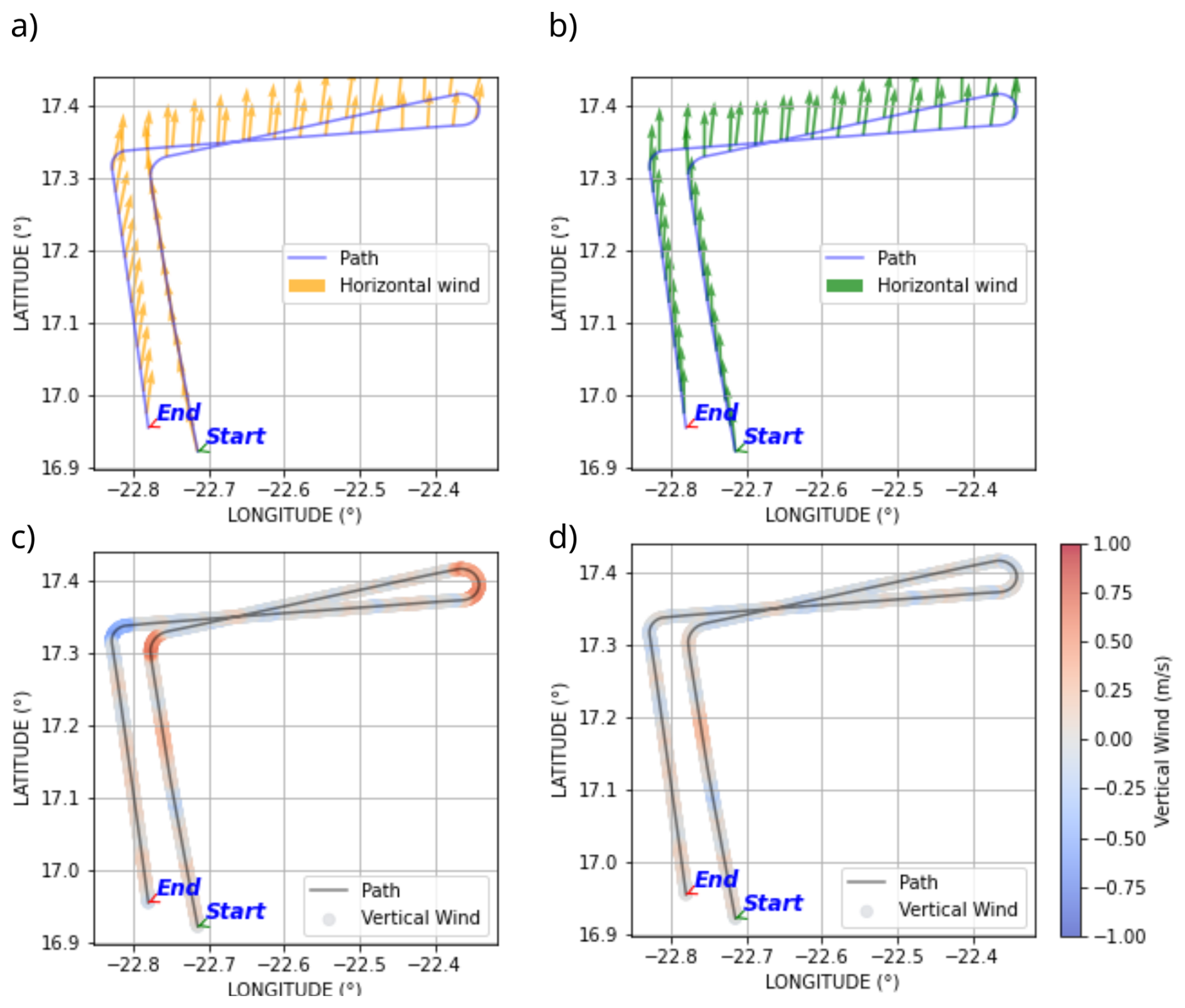
Figure A1 Computed wind vectors during the reverse heading maneuver with and without wind corrections. Initially computed horizontal (a) and vertical (c) winds along the plane's trajectory. Corrected horizontal (b) and vertical (d) winds along the plane's trajectory. This maneuvers took place during RF22 on 7 September 2024.

Appendix B: Intercomparison of humidity reference sensors

This analysis evaluates reference instruments against their known limitations and examines their mutual agreement under varying atmospheric conditions. In principle, the 1011C chilled-mirror hygrometer provides the most accurate humidity measurement available on the ATR-42, as it directly measures dew point temperature through condensation/evaporation rather than relying on calibrated spectroscopic or capacitive responses. This makes it the natural reference for evaluating the other instruments. However, its thermal response time (limited to 1 K s⁻¹ warming rate) constrains its ability to track rapid humidity changes. In heterogeneous atmospheric conditions, this limitation can introduce systematic errors, as discussed below. The WVSS-2 is a calibrated laser absorption spectrometer with negligible response time, while the HUMAERO is a calibrated capacitive sensor sensitive to relative humidity, which is then converted to mixing ratio using an associated temperature measurement. Unlike the 1011C, both the WVSS-2 and HUMAERO acquire independent, near-instantaneous measurements at each sampling point.

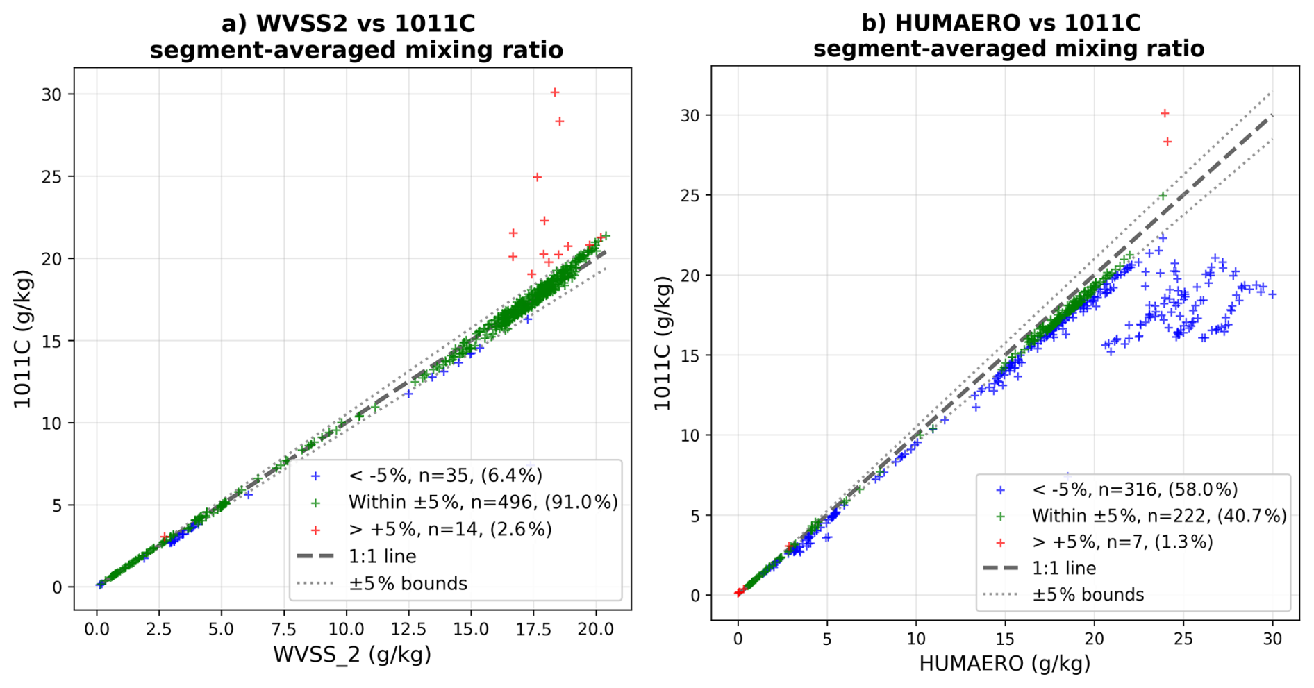
Figure B1 Comparison of mixing ratio values averaged over segments for the WVSS-2 (a) and HUMAERO (b) with respect to the 1011C instrument. In green, points where instruments agree within ± 5 %, in blue points where the 1011C measurements are lower by more than 5 %, and in red higher than 5 %.

Figure B1 compares segment-averaged mixing ratio values from the WVSS-2 and HUMAERO against those from the 1011C. The WVSS-2 agrees with the 1011C within ± 5 % for 509 segments (90.4 % of the dataset), whereas the HUMAERO agrees for only 236 segments (41.9 %). The HUMAERO systematically overestimates mixing ratio by more than 5 % in 317 segments (56.3 %). In contrast, the WVSS-2 shows excellent agreement across nearly all segment types, with deviations primarily confined to specific conditions (ice clouds and high-humidity segments) that can be physically explained (see below). Given that the majority of segments were acquired in clear-sky conditions, where the 1011C's thermal inertia is less problematic and its measurements are expected to be accurate, the underestimation by the HUMAERO cannot be attributed to limitations of the reference instrument. The capacitive sensor's conversion from relative humidity to mixing ratio also introduces additional uncertainty through its dependence on accurate temperature measurement and calibration stability under varying ambient conditions. Based on this evidence, the HUMAERO is excluded from further consideration as a reliable reference sensor for the MAESTRO dataset.

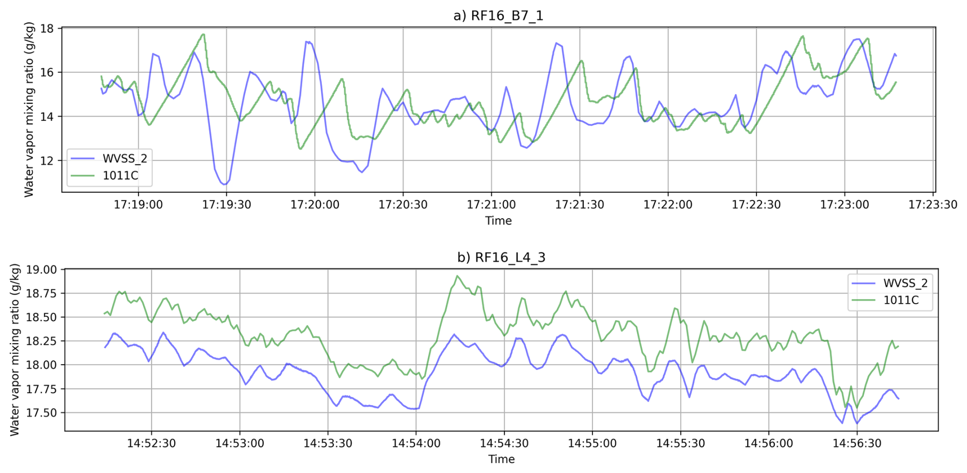
Figure B2 Example of mixing ratio time series from the 1011C and WVSS-2 instruments, showing ramping structures due to the relatively slow warming rate of the 1011C, compared with instantaneous recording of laser absorption from the WVSS-2 for a B-type segment (a) with cloud encounters and a clear sky L-type segment (b) from the same RF16 flight.

Figure B2 shows example time series from one of the mixed layer segments and one of the cloud base segments for the two remaining reference sensors (WVSS-2 and 1011C). The 1011C exhibits clear ramping phases when adapting to higher humidity/dew point values, while it cools down rapidly to measure negative humidity gradients thanks to the strong airstream. This asymmetric response to positive and negative humidity gradients causes a systematic underestimation of the average mixing ratio during such segments where local heterogeneity of the moisture field exceeds the adaptation capacity of the mirror. Figure B3 shows average values for each segment, obtained from the two reference sensors and sorted by segment type. Most cloud base segments (in green) fall below the 1:1 line, reflecting the fact that the behavior described in Fig. B2. Conversely, L-type segments generally lie slightly above the 1:1 line. These latter segments are very moist and approach the edge of the WVSS-2 calibration range. Similar issues may affect B-types as well.

Within the 36 segments (6.4 % of the dataset) for which the WVSS-2 values exceed those of the 1011C by more than 5 %, 26 belong to saturated H-type segments (traversing ice or mixed phase clouds), 6 to B-type segments, and 4 to M-type segments. When the deviation threshold is narrowed to 2 %, 109 segments exhibit deviations below this threshold, including 59 B-type, 39 H-type, 3 T-type, and 8 M-type segments. These results support the sustained hypothesis, attributing the disagreement between the WVSS-2 and 1011C to limitations of the 1011C rather than overestimation by the WVSS-2. Of the 18 segments for which the 1011C measured significantly higher mixing ratios compared to the WVSS-2, 14 belong to the B-type, 1 each to the H- and S-types, and 2 to the L-type. These segments are characterized by high relative humidities or cloud fraction. Inspection of these few anomalous segments reveals large mixing ratio jumps exceeding 10 g kg⁻¹ in the 1011C signal that strongly affect the mean values. Although we cannot provide a physical explanation for this behavior, an environmental origin is ruled out, as none of the other five instruments recorded similar patterns, and such variability is not expected in the atmosphere. No post-processing correction was applied to compensate for the 1011C's thermal inertia. Inversion techniques to correct for the limited warming rate (1 K s⁻¹) would likely introduce additional uncertainty in particular when combined with the calibration of fast sensors. Instead, we account for this limitation by selecting WVSS-2 as the primary reference, which combines robustness and high accuracy under all MAESTRO conditions.

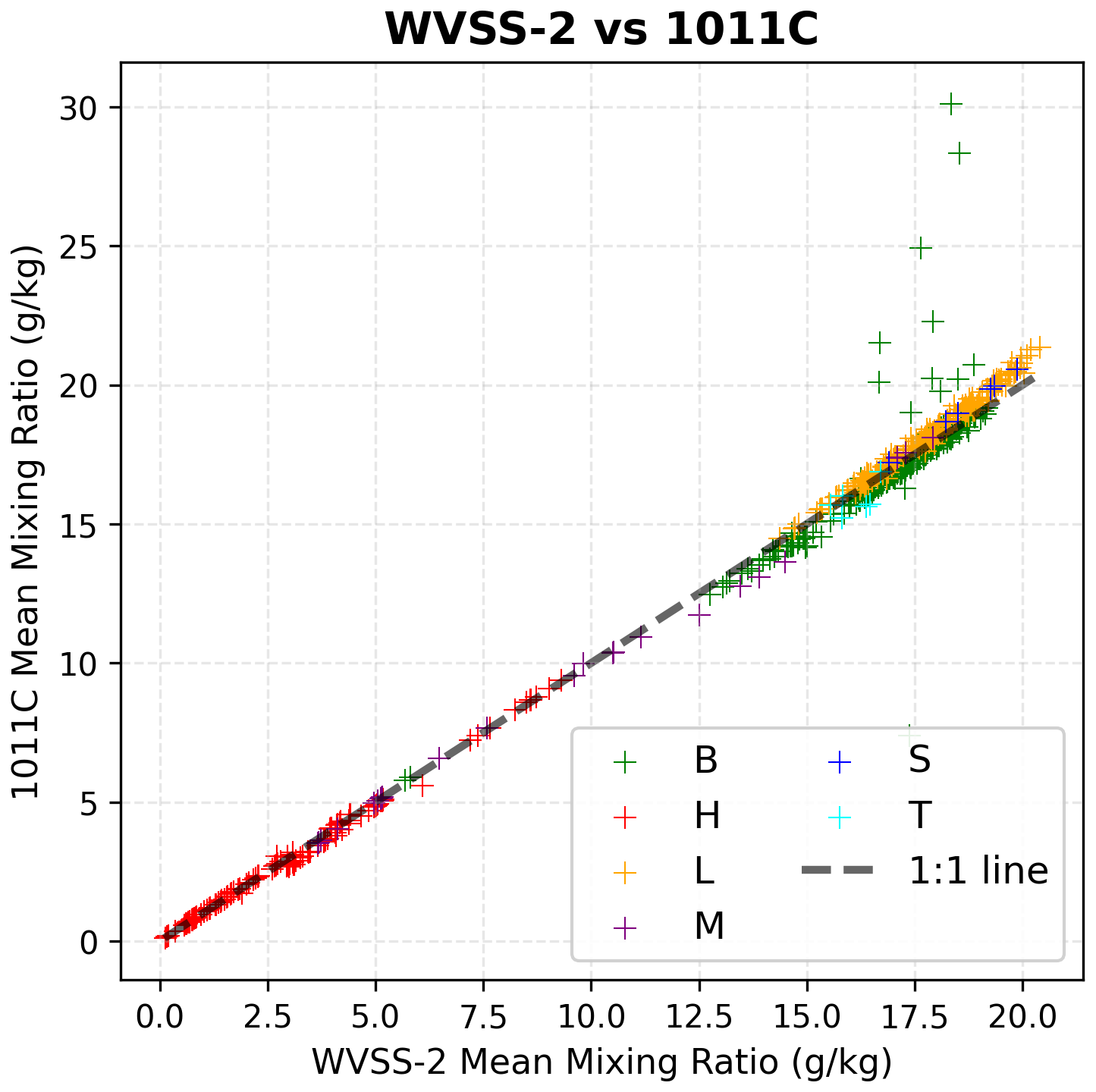
Figure B3 Comparison of mixing ratio values averaged over segments for the 1011C and WVSS-2, by segments types.