Daily global sea surface ageostrophic current dataset from 1993–2023 via physics-informed deep learning

Surface ocean circulation shapes climate, air–sea exchange, and the transport of heat, carbon, and other tracers, yet most long-term global datasets rely primarily on geostrophic balance and therefore miss important ageostrophic motions. Here, we reconstruct global daily sea surface circulation at 0.25° resolution from 1993 to 2023 using a physics-informed framework that integrates satellite altimetry with momentum constraints from geostrophic balance, wind stress, and nonlinear advection (Cui, 2026; https://doi.org/10.5281/zenodo.19966716). The resulting dataset is dynamically consistent, with a mean momentum balance error below 1.5 %, and reduces the median velocity error against independent mooring observations across the tropical Pacific, Atlantic, and Indian Oceans to 0.07 m s⁻¹, compared with 0.20 m s⁻¹ for geostrophic currents and 0.10 m s⁻¹ for Ekman corrected currents. We show that geostrophic flow sets the large-scale circulation, whereas Ekman and nonlinear contributions are smaller but comparable in magnitude to each other. Although nonlinear advection contributes little to relative vorticity, it strongly shapes surface divergence and the fine scale structure of eddy kinetic energy. Our results show that nonlinear ageostrophic flow is an essential component of global surface circulation and that neglecting it limits our ability to resolve surface transport and variability on climatically relevant scales.

1 Introduction

Surface ocean circulation regulates climate, air–sea exchange, and the transport of heat, carbon, nutrients, and other tracers. Over the past several decades, satellite remote sensing has provided the principal observational basis for studying upper ocean circulation (Du et al., 2021; Fan et al., 2025; Shang et al., 2025). Geostrophic currents derived from sea surface height have become central to analyses of ocean dynamics (Wunsch and Gaposchkin, 1980), climate change, and ecosystem assessments (Timmermans and Marshall, 2020; Srinivasan and Tsontos, 2023). However, geostrophic currents neglect the influence of ageostrophic processes, such as wind stress and nonlinear effects (Hiron et al., 2021). Although ageostrophic processes are relatively small in magnitude, both observational data and numerical simulations have consistently shown that they substantially modulate ocean circulation (Rio et al., 2014; Edwards et al., 2024). Ageostrophic motions play a crucial role in the evolution and adjustment of ocean circulation. For example, nonlinear effects contribute to the evolution of mesoscale eddies (Li et al., 2022) and are important for the transport of heat, dissolved carbon, and tracers (Ueno et al., 2023; Dong et al., 2020). Studies have also shown that nonlinear processes can reduce geostrophic current speeds by more than 0.2 m s⁻¹ (Cao et al., 2023b), whereas wind-driven Ekman effects can enhance sea surface current velocities (Rio et al., 2014). Neglecting ageostrophic processes (Armitage et al., 2017; Shankar et al., 2002; Cho et al., 2025) omits the complex features introduced by variations in nonlinear forcing and wind stress (Andres et al., 2008; Buckingham et al., 2021), leading to substantial discrepancies with drifter observed velocities (Douglass and Richman, 2015; Uchida and Imawaki, 2003). This omission introduces uncertainties in understanding the long-term evolution and energy transformation of ocean circulation.

The influence of ageostrophic motions is especially pronounced in energetically active regions such as western boundary currents, the subtropical countercurrent, and the Antarctic Circumpolar Current, where their kinetic energy can be comparable to that of geostrophic motions (Zhang et al., 2019). The development of ageostrophic motions can disrupt geostrophic balance, promote forward energy transfer, and influence the inverse transfer of geostrophic energy, leading to an increase in the mean geostrophic wavenumber (Kafiabad et al., 2019; Thomas and Daniel, 2021). Ageostrophic motions are also closely linked to marine ecosystems: the intense vertical motions they induce provide an important pathway for delivering nutrients into the euphotic zone and thereby help regulate primary productivity and carbon sequestration in the global ocean (Aluie et al., 2018; Liu et al., 2025; Masuda et al., 2021).

Most existing corrections to sea surface circulation adopt a steady state framework (Fraser et al., 2024), and two main methods are commonly used to represent nonlinear effects. One assumes axisymmetric vortices and reduces nonlinear forcing to the centrifugal term in the gradient wind equation (Ioannou et al., 2019). The other uses a perturbation expansion in which the nonlinear term is approximated by the rate of change of geostrophic velocity (Penven et al., 2014). In practice, most previous studies have used iterative schemes for circulation correction (Cao et al., 2023a; Penven et al., 2014). The iterative solution of the gradient wind equation was first developed in atmospheric science (Penven et al., 2014; Gold, 1908) and later introduced into oceanography. Such schemes have been applied to a large gyre in the Mozambique Channel, mesoscale eddies in the Mediterranean Sea (Cao et al., 2023a; Penven et al., 2014; Morales-Márquez et al., 2023), and the correction of the global sea surface circulation field (Cao et al., 2023b; Ruiz et al., 2014). However, these schemes can diverge when the gradient wind equation has no solution (Douglass and Richman, 2015; Qiu et al., 2019). Furthermore, the stopping criterion for these schemes is typically when the velocity residual either begins to diverge or decreases below a predefined threshold (Douglass and Richman, 2015; Qiu et al., 2019), which is commonly set to 0.01 m s⁻¹ in the literature (Cao et al., 2023a; Arnason et al., 1962; Penven et al., 2014). As a result, the dynamical consistency of the corrected solution remains uncertain.

Recent advances in artificial intelligence (AI) have created new opportunities for oceanographic data analysis and reconstruction (Li et al., 2020; Dong et al., 2022; Qin et al., 2023; Cui et al., 2025). AI has been applied to infer ocean surface dynamic parameters and structures (Bonino et al., 2024; Jang et al., 2022; Cui et al., 2026; Lenain et al., 2026), such as subsurface eddy kinetic energy (Cai and Gan, 2021; Dong et al., 2021) , subsurface thermohaline structure (Zhou et al., 2024), and sea surface temperature (Bonino et al., 2024; Kumar et al., 2021; Kartal, 2023). AI based research on sea surface circulation is also beginning to emerge. Existing work primarily uses machine learning to replace traditional geostrophic relationships by combining satellite observed variables, such as sea surface height, sea surface temperature, and wind stress, to reconstruct global sea surface circulation fields (Sinha and Abernathey, 2021; Manucharyan et al., 2021). However, these approaches do not fully integrate the governing physical equations of ocean surface circulation into the learning framework for ageostrophic correction. As a result, the reconstructed flow fields can retain non-negligible dynamical imbalances, as reflected in residual terms of the momentum equations.

Here, we develop a physics informed density neural network with ageostrophic circulation correction (AC-PIDNN) to reconstruct global sea surface circulation while explicitly enforcing momentum balance. The model integrates constraints from geostrophic balance, wind stress, and nonlinear advection to recover ageostrophic flow from satellite observed sea surface height gradients. Using the AC-PIDNN, we generate a daily global ageostrophic current dataset from 1993 to 2023 at a spatial resolution of 0.25°. This framework enables a dynamically consistent assessment of how ageostrophic processes shape global surface circulation, divergence, and eddy energetics. The structure of this paper is as follows: Sect. 2 describes the data used; Sect. 3 introduces the proposed methodology; Sect. 4 presents the experimental results and discussions; Sects. 5 and 6 present the code and data availability and conclusions, respectively.

2 Data

2.1 Satellite data

The dataset used in this study includes the daily Absolute Dynamic Topography (ADT) gridded data, geostrophic currents ${\mathit{V}}_{\text{geo}}=(u_{\text{geo}},v_{\text{geo}})$, and the corresponding surface Ekman components of the global ocean, which were downloaded from https://data.marine.copernicus.eu/product (last access: 3 November 2026). The ADT gridded data are processed by SSALTO/DUACS and distributed by AVISO (https://www.aviso.altimetry.fr, last access: 3 November 2026) supported by CNES (CNES and CLS, 2025). This system integrates observations from all Sentinel altimetry missions as well as other collaborative or opportunistic missions. The datasets incorporate high quality altimeter measurements and geophysical corrections and are generated using a consistent correction system to ensure maximum data quality and to minimize temporal artifacts. This dataset also provides geostrophic current V_geo based on the geostrophic balance. These data used in this study have a temporal resolution of 1 d and a spatial resolution of $\mathrm{1}/\mathrm{4}$°.

The surface Ekman components are obtained from the global Copernicus Ocean (GLOBCURRENT) surface and 15 m Ekman and geostrophic current datasets (Mulet et al., 2021; Rio et al., 2014). These data are derived by applying an empirical Ekman model to ERA5 wind stress fields, with the calculation taking into account both wind stress and the mixed layer depth. The inclusion of mixed layer depth reflects the dynamic variability of Ekman depth across time and space. This product provides datasets on a $\mathrm{1}/\mathrm{4}$° regular grid, offering current velocity fields at the surface and at 15 m depth with hourly, daily, and monthly temporal resolutions.

2.2 Simulation data

To provide an additional evaluation of the performance of the proposed method, we conducted a high resolution numerical simulation using the Regional Ocean Modeling System (ROMS) (Shchepetkin and Mcwilliams, 2005), which served as a supplementary and physically consistent reference for further assessing the effectiveness of our approach. ROMS is a widely used, high resolution numerical framework designed for simulating regional scale oceanic and atmospheric processes. By solving the governing equations of fluid motion, ROMS provides accurate simulations of ocean circulation, temperature, salinity, and other essential physical properties while maintaining strong dynamical consistency and numerical stability. In this study, the simulation configuration covers the western Pacific region (5–32° N, 109–141° E) (Chen et al., 2026) with a spatial resolution of 3 km, allowing the model to resolve mesoscale circulation features. The model was initialized using horizontally uniform temperature and salinity fields derived from the annual mean World Ocean Atlas 2013 data averaged over the North Pacific Ocean. The large scale circulation was driven by prescribed mean external volume fluxes at the southeastern and northeastern open boundaries, respectively, and no observational data were assimilated during the simulation. Following initialization, the model was integrated for 25 years, and the final 5 years of the simulation were used for analysis. The ROMS fields used in this study were averaged over 30 d to provide a more stable representation of the regional circulation for comparison. It also forms a foundation for further investigation of regional circulation characteristics and underlying dynamical mechanisms.

3 Methodology

3.1 The steady state momentum balance equations

In this study, the surface sea currents within the Ekman layer are assumed satisfy the steady state momentum balance between nonlinear advection, pressure gradient force, Coriolis force and wind stress (Sudre et al., 2013; Van Meurs and Niiler, 1997):

$$\begin{array}{}\text{(1)}& {\displaystyle }& {\displaystyle }\stackrel{{\text{ADV}}_x}{\overbrace{u{\displaystyle \frac{\partial u}{\partial x}}+v{\displaystyle \frac{\partial u}{\partial y}}}}=\stackrel{{\text{COR}}_x}{\overbrace{fv}}\stackrel{{\text{PGF}}_x}{\overbrace{-g{\displaystyle \frac{\partial \mathit{\eta }}{\partial x}}}}+\stackrel{{\text{WIND}}_x}{\overbrace{{\displaystyle \frac{\mathrm{1}}{h_{\mathrm{e}}}}\left({\displaystyle \frac{{\mathit{\tau }}_x}{\mathit{\rho }}}-r_{\mathrm{e}}{u}_{\text{ekman}}\right)}}\text{(2)}& {\displaystyle }& {\displaystyle }\stackrel{{\text{ADV}}_y}{\overbrace{u{\displaystyle \frac{\partial v}{\partial x}}+v{\displaystyle \frac{\partial v}{\partial y}}}}=\stackrel{{\text{COR}}_y}{\overbrace{-fu}}\stackrel{{\text{PGF}}_y}{\overbrace{-g{\displaystyle \frac{\partial \mathit{\eta }}{\partial y}}}}+\stackrel{{\text{WIND}}_y}{\overbrace{{\displaystyle \frac{\mathrm{1}}{h_{\mathrm{e}}}}\left({\displaystyle \frac{{\mathit{\tau }}_y}{\mathit{\rho }}}-r_{\mathrm{e}}{v}_{\text{ekman}}\right)}}\end{array}$$

where, u and v are the zonal and meridional velocities; η is the sea surface height from ADT data; f represents the Coriolis force parameter; g is gravity acceleration; and τ(τ_x,τ_y) is the wind stress field. The h_e and r_e are thickness of the Ekman layer and the linear drag coefficient that represents the vertical viscosity terms as a body force on the Ekman components. With the information from the locally estimated h_e and r_e, the ${\mathit{V}}_{\text{ekman}}=(u_{\text{ekamn}},v_{\text{ekamn}})$, can be calculated based on the wind stress field. In our calculation, the $\stackrel{{\text{WIND}}_x}{\overbrace{\frac{\mathrm{1}}{h_{\mathrm{e}}}\left(\frac{{\mathit{\tau }}_x}{\mathit{\rho }}-r_{\mathrm{e}}{u}_{\text{ekman}}\right)}}$ and $\stackrel{{\text{WIND}}_y}{\overbrace{\frac{\mathrm{1}}{h_{\mathrm{e}}}\left(\frac{{\mathit{\tau }}_y}{\mathit{\rho }}-r_{\mathrm{e}}{v}_{\text{ekman}}\right)}}$ are represented by the −fv_ekman and fu_ekman, in which u_ekman and v_ekman are the Ekman component of current in GLOBCURRENT data to simplify the calculation.

3.2 Physics informed density neural networks for correcting ageostrophic current (AC-PIDNN)

In this study, we propose a physics informed neural network (PINN) based architecture for correcting ageostrophic current, termed AC-PIDNN. The overall structure, as shown in Fig. 1, consists of three components: input module, custom density neural networks module, and loss function module.

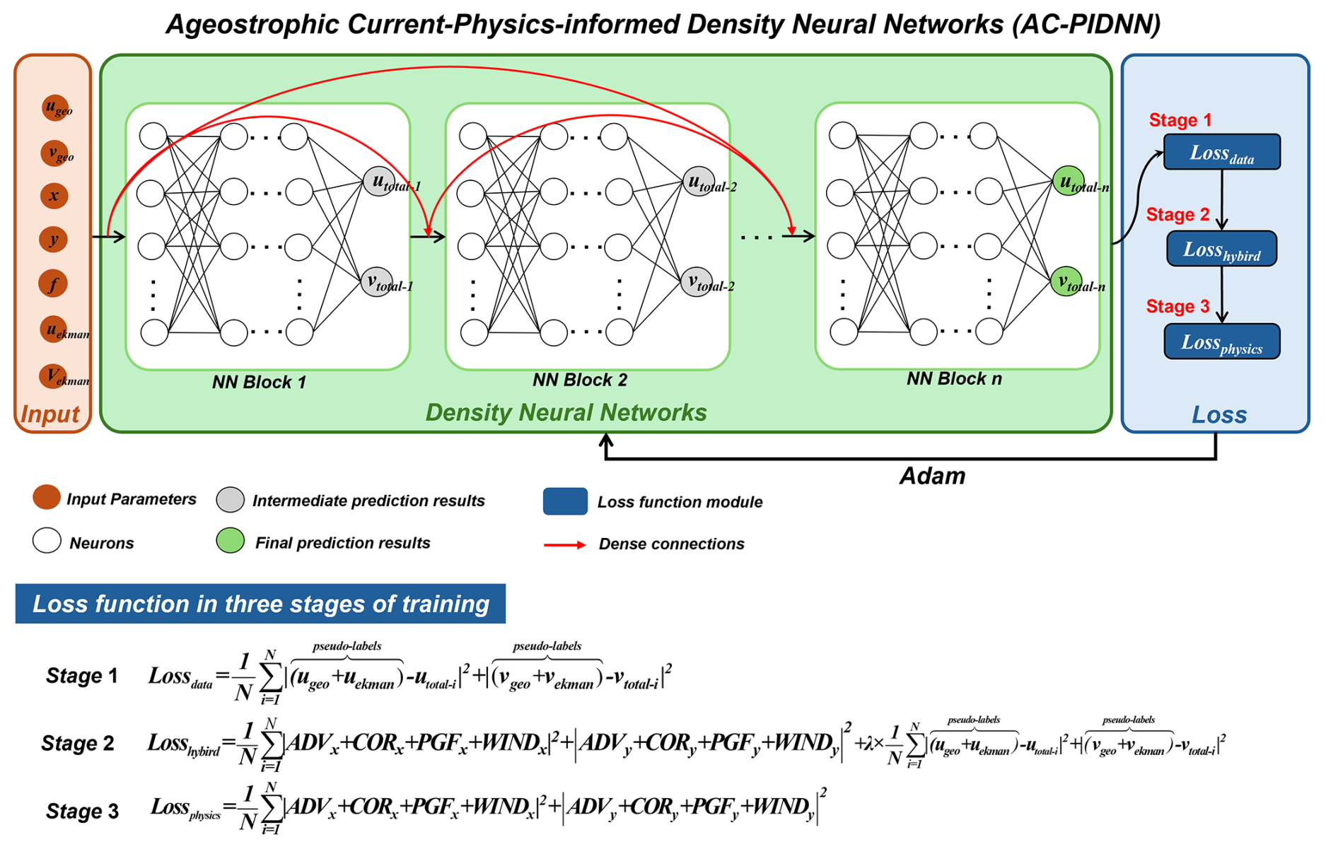
Figure 1 Schematic diagram of the proposed sea surface circulation correction model (AC-PIDNN).

3.2.1 Input module

The model inputs include geostrophic current components derived from the geostrophic approximation (u_geo,v_geo), surface Ekman current components (u_ekman,v_ekman), Coriolis parameter f, and geographical coordinates (x,y). The input features be represented as:

$$\begin{array}{}\text{(3)}& \mathbf{X}=\left[u_{\text{geo}},v_{\text{geo}},x,y,f,u_{\text{ekman}},v_{\text{ekman}}\right]\end{array}$$

The geostrophic currents are calculated based on the geostrophic balance:

$$\begin{array}{}\text{(4)}& {\displaystyle }& {\displaystyle }f{v}_{\text{geo}}-g{\displaystyle \frac{\partial \mathit{\eta }}{\partial x}}=\mathrm{0}\text{(5)}& {\displaystyle }& {\displaystyle }-f{u}_{\text{geo}}-g{\displaystyle \frac{\partial \mathit{\eta }}{\partial y}}=\mathrm{0}\end{array}$$

In this study, u_geo and v_geo are directly derived from the AVISO dataset. However, Eqs. (4) and (5) become singular at the equator (f=0), and they are also problematic in its vicinity due to the weak Coriolis effect. To address this issue, within the latitude band of ± 2°, this study adopts the so-called “semi-geostrophic” approximation to compute the equatorial current components ${\mathit{V}}_{\text{sg}}=(u_{\text{sg}},v_{\text{sg}})$, which replace the geostrophic currents in this region (Sudre et al., 2013):

$$\begin{array}{}\text{(6)}& {\displaystyle }& {\displaystyle }{u}_{\text{sg}}=-{\displaystyle \frac{g}{\mathit{\beta }}}{\displaystyle \frac{{\partial }^{\mathrm{2}}\mathit{\eta }}{\partial y^{\mathrm{2}}}}\text{(7)}& {\displaystyle }& {\displaystyle }{v}_{\text{sg}}={\displaystyle \frac{g}{\mathit{\beta }}}{\displaystyle \frac{{\partial }^{\mathrm{2}}\mathit{\eta }}{\partial x^{\mathrm{2}}}}\end{array}$$

where β is the meridional gradient of the Coriolis parameter, defined as $\mathit{\beta }=\frac{\mathrm{2}\mathrm{\Omega }\text{cos}\mathit{\phi }}{R}$, Ω is the Earth's angular velocity of rotation, φ is the latitude, R is the Earth's radius.

3.2.2 Density neural networks module

The Density Neural Networks module incorporates multiple fully connected neural network (NN) layers, organized into NN submodules, and employs residual connections similar to ResNet (He et al., 2016) to facilitate efficient information transfer between modules. This design aims to minimize the loss of information from the initial geostrophic current field during feature extraction and to accelerate model convergence and enhance stability. The AC-PIDNN architecture employs three NN blocks, each containing five hidden layers with 100 neurons per layer. Each NN block consists of a sequence of fully connected transformations:

$$\begin{array}{}\text{(8)}& h^{\left(l\right)}=\mathit{\sigma }\left(W^{\left(l\right)}{h}^{(l-\mathrm{1})}+b^{\left(l\right)}\right),l=\mathrm{1},\mathrm{\dots },L\end{array}$$

where h⁽⁰⁾=X, W^(l) and b^(l) are the trainable weights and biases of the lth layer, σ(⋅) denotes the activation function, and L is the number of hidden layers in each block. To preserve the physical meaning of the geostrophic input and reduce the loss of dynamical information, a residual connection is applied:

$$\begin{array}{}\text{(9)}& h^{\left(l\right)}=f\left(h^{\left(l\right)}\right)+h^{(l-\mathrm{1})}\end{array}$$

This residual mechanism allows the NN block to learn corrections to the geostrophic current field rather than relearning it from scratch. From a physical perspective, the predicted current field ${\mathit{V}}_{\text{total}}=(u_{\text{total}},v_{\text{total}})$ can be expressed as the sum of the geostrophic component and a correction term:

$$\begin{array}{}\text{(10)}& {\displaystyle }& {\displaystyle }{u}_{\text{total}}=u_{\text{geo}}+\mathrm{\Delta }u(\mathbf{X};\mathit{\theta })\text{(11)}& {\displaystyle }& {\displaystyle }{v}_{\text{total}}=v_{\text{geo}}+\mathrm{\Delta }v(\mathbf{X};\mathit{\theta })\end{array}$$

where Δu and Δv are the data driven corrections parameterized by the network weights θ. This formulation ensures that the essential dynamical information from the geostrophic approximation is retained while enabling the network to learn the ageostrophic corrections. Consequently, the residual structure accelerates convergence, improves gradient stability during backpropagation, and prevents the model from overfitting to spurious patterns in the training data.

3.2.3 Loss function module and training strategy

The loss function module consists of three customized loss functions. To address this and eliminate the need for manual hyperparameter tuning (e.g., grid search), we implemented an adaptive loss scaling mechanism during the Stage 2 hybrid training.

$$\begin{array}{}\text{(12)}& {\displaystyle }\begin{array}{rl}{\text{Loss}}_{\text{data}}=& {\displaystyle \frac{\mathrm{1}}{N}}\sum _{i=\mathrm{1}}^N\mathrm{|}{u}_{\text{Pseudo\hspace{0.17em}\hspace{0.17em}labels}}-u_{\text{total}-i}{\mathrm{|}}^{\mathrm{2}}\\ & +\mathrm{|}{v}_{\text{Pseudo\hspace{0.17em}\hspace{0.17em}labels}}-v_{\text{total}-i}{\mathrm{|}}^{\mathrm{2}}\end{array}\text{(13)}& {\displaystyle }\begin{array}{rl}{\text{Loss}}_{\text{physics}}=& {\displaystyle \frac{\mathrm{1}}{N}}\sum _{i=\mathrm{1}}^N\mathrm{|}{\text{ADV}}_x+{\text{COR}}_x+{\text{PGF}}_x\\ & +{\text{WIND}}_x{\mathrm{|}}^{\mathrm{2}}+\mathrm{|}{\text{ADV}}_y+{\text{COR}}_y\\ & +{\text{PGF}}_y+{\text{WIND}}_y{\mathrm{|}}^{\mathrm{2}}\end{array}\text{(14)}& {\displaystyle }{\text{Loss}}_{\text{hybird}}={\text{Loss}}_{\text{data}}+\mathit{\lambda }\times {\text{Loss}}_{\text{physics}}\end{array}$$

Here, N denotes the number of training samples; ${\mathit{V}}_{\text{Pseudo\hspace{0.17em}\hspace{0.17em}labels}}=(u_{\text{Pseudo\hspace{0.17em}\hspace{0.17em}labels}},v_{\text{Pseudo\hspace{0.17em}\hspace{0.17em}labels}})$ represents the pseudo labels for model initialization, which are constructed using the sum of the corresponding geostrophic and Ekman components; and ${\mathit{V}}_{\text{total}-i}=(u_{\text{total}-i},v_{\text{total}-i})$ are the model-predicted current components in the ith epoch; Loss_data represents the mean squared error between the predicted and pseudo label constructed from the geostrophic current plus the Ekman current, and is used for initial model fitting; Loss_physics measures the residuals of the predicted current field in the momentum equations, constraining the outputs to satisfy the two dimensional momentum balance as closely as possible; It is worth noting that the Loss_physics is calculated for each predicted ($u_{\text{total}-i},v_{\text{total}-i}$), which is dynamic value. Loss_hybird is a weighted combination of the above two, enabling a smooth transition from data-driven to physics-driven learning by gradually increasing the weight of physical constraints during training. The adaptive weight λ is calculated as $\mathit{\lambda }=sg\left(\frac{L_{\text{data}}}{L_{\text{physics}}}\right)$. Here, sg(⋅) denotes the stop gradient operation, ensuring that the weight acts only as a scaling factor and does not interfere with the backpropagation process. This mechanism maintains a 1:1 balance between data and momentum constraints throughout the training, ensuring robustness and reproducibility.

The adaptive optimization algorithm Adam (Kingma and Ba, 2014) is employed to minimize the loss function, and neural network parameters are initialized using the Xavier scheme (Xavier et al., 2025). The hyperbolic tangent (tanh) is adopted as the activation function. Furthermore, L₂ regularization and dropout are utilized to mitigate overfitting, with each serving distinct physical roles within the architecture. Once training converges and the loss function reaches a sufficiently small value, the predicted (u_total,v_total) values approximate the solutions of the Eqs. (1) and (2). To ensure stability and accuracy, a three stage training strategy is adopted:

Stage 1 data driven initialization, using only Loss_data (learning rate = 0.001, epochs = 1000). This allows the model to rapidly capture the macroscopic features of the geostrophic and Ekman flows. It establishes a physically reasonable starting point, preventing the non-uniqueness problem that occurs when starting from random initialization.

Stage 2 transitional hybrid optimization, using Loss_hybird (learning rate = 0.0001, epochs = 1000). Enforcing strong physical constraints too abruptly can cause gradient instability. This hybrid stage acts as a buffer, gently introducing momentum balance constraints to guide the model away from purely data fitted local minima.

Stage 3 pure physics refinement, using only Loss_physics (learning rate = 0.00001, epochs = 10 000). By removing the data constraint, we allow the network to minimize the momentum residuals strictly. Because the model is already anchored in a realistic state by Stages 1 and 2, minimizing Loss_physics does not lead to an arbitrary solution; instead, it accurately isolates and resolves the nonlinear dynamical components that cannot be captured by data fitting alone. During this stage, the spatial derivatives required for the advective terms within the momentum equations are evaluated via automatic differentiation of the network outputs with respect to the input coordinates (x,y). This approach leverages the continuous differentiability of the neural network to calculate velocity gradients more precisely than traditional finite difference methods.

Notably, to successfully isolate the ageostrophic components from the momentum equations, the combined geostrophic and Ekman flow components are utilized as pseudo labels during Stages 1 and 2. Subsequently, Stage 3 relies entirely on physical constraints to execute the separation of the ageostrophic components. Detailed parameter configurations for the proposed AC-PIDNN model are provided in Table S1 in the Supplement.

3.3 Ageostrophic current component decomposition

The ocean current field V_total predicted by PINN contains the component of geostrophy (V_geo), wind stress (V_ekman), and nonlinearity (V_adv):

$$\begin{array}{}\text{(15)}& {\mathit{V}}_{\text{total}}={\mathit{V}}_{\text{geo}}+{\mathit{V}}_{\text{adv}}+{\mathit{V}}_{\text{ekman}}\end{array}$$

Where V_total is the velocity vector predicted by AC-PIDNN, V_geo is the geostrophic current from AVISO data and V_ekman is surface Ekman current in GLOBCURRENT data. Thus, the ADV, COR and WIND effect in Eqs. (1) and (2) is represented as fk×V_adv, fk×V_total, and fk×V_ekman. To verify the balance of the predicted u_total and v_total from AC-PIDNN, the following balance was examined:

$$\begin{array}{}\text{(16)}& {\displaystyle }{\text{Bal}}_x={\text{COR}}_x+{\text{PGF}}_x+{\text{WIND}}_x+{\text{ADV}}_x\text{(17)}& {\displaystyle }{\text{Bal}}_y={\text{COR}}_y+{\text{PGF}}_y+{\text{WIND}}_y+{\text{ADV}}_y\text{(18)}& {\displaystyle }\text{Bal}={\left({\left({\displaystyle \frac{{\text{Bal}}_x}{{\text{PGF}}_x}}\right)}^{\mathrm{2}}+{\left({\displaystyle \frac{{\text{Bal}}_y}{{\text{PGF}}_y}}\right)}^{\mathrm{2}}\right)}^{\frac{\mathrm{1}}{\mathrm{2}}}\end{array}$$

Which quantifies the normalized residual of the balance in Eqs. (1) and (2). It is worth noting that, the Bal in this study is not intended as an independent external validation metric, but rather as a core self-consistency standard ensuring internal physical consistency. The minimization of this residual strictly validates that the extracted nonlinear advection terms satisfy the physical equation constraints.

4 Results and discussions

4.1 Validation of reconstructed currents and dynamical consistency

4.1.1 Dynamical consistency

This study employed the AC-PIDNN to reconstruct the daily global sea surface circulation from 1993 to 2023, incorporating geostrophic, nonlinear advective and Ekman corrected components. The 30-year mean dynamical consistency of the AC-PIDNN reconstructed surface circulation was evaluated by examining the zonal (Bal_x) and meridional (Bal_y) balances, together with the ratio of the residual magnitude to the pressure gradient force (Bal) (Fig. 2a–c). The residuals are generally small over most of the global ocean, with typical magnitudes on the order of 10⁻⁶ m s⁻². Relatively larger residuals are mainly confined to regions characterized by strong currents and energetic mesoscale variability, including western boundary current extensions and parts of the Southern Ocean. Despite these localized enhancements, the overall balance index Bal remains below 5 %, indicating that the reconstructed surface circulation satisfies the surface momentum balance to a high degree across the global ocean. The Fig. 2d illustrates the temporal evolution of the globally averaged Bal from 1993 to 2023. The global mean value remains stable over the entire period, with the global mean ± standard deviation range varies between 1 %–1.5 %. No systematic drift or long-term trend is evident, demonstrating that the correction maintains a consistent level of dynamical balance throughout the multi-decadal record. Figures S1 and S2 in the Supplement show the momentum balance (Bal) evolution from Stage 1 to Stage 3 of the AC-PIDNN model's training, as well as comparisons with in situ measurements and the Ocean Surface Current Analyses Real-time (OSCAR) dataset (ESR and Dohan, 2022), validating the strong accuracy of the AC-PIDNN corrections. Together, these results confirm that the AC-PIDNN correction yields a surface circulation that is dynamically self-consistent and temporally robust.

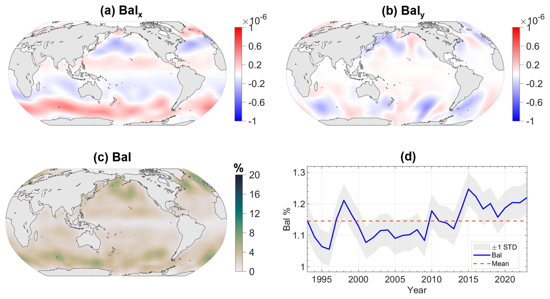
Figure 2 Balance analysis of the corrected 30-year means flow field within the momentum equations Eqs. (4) and (5). (a) 30-year mean residual of the zonal momentum equation, Bal_x (m s⁻²), from 1993 to 2023; (b) 30-year mean residual of the meridional momentum equation, Bal_y (m s⁻²), from 1993 to 2023; (c) 30-year mean ratio of the magnitude of the momentum equation residuals to the pressure gradient force, Bal, from 1993 to 2023. (d) Time evolution of the globally averaged Bal from 1993 to 2023, with the shaded area representing the ± 1 standard deviation range.

4.1.2 Comparison of AC-PIDNN corrected flow fields and OSCAR Products against in situ data

To comprehensively validate the reliability and applicability of the AC-PIDNN dataset across different dynamical regimes globally, a systematic evaluation was conducted using widespread in situ observations, alongside a multi-region comparative analysis with the existing OSCAR surface current product (1993–2022) downloaded from https://doi.org/10.5067/OSCAR-25F20 (ESR and Dohan, 2021). The in situ data used for validation are derived from the tropical mooring buoy arrays, comprising the TAO array in the Pacific Ocean, the PIRATA array in the Atlantic Ocean, and the RAMA array in the Indian Ocean. As shown in Fig. 3a, a total of 54 observation stations widely distributed across the Pacific Ocean (21 stations), Atlantic Ocean (14 stations), and Indian Oceans (19 stations) (downloaded from https://www.pmel.noaa.gov/tao/drupal/disdel/, last access: 3 November 2026).

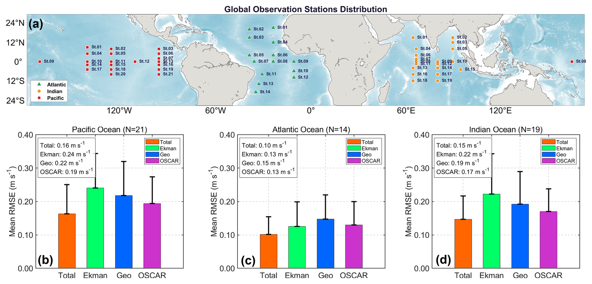
Figure 3 (a) Spatial distribution of TAO/PIRATA/RAMA mooring sites across the Pacific, Atlantic, and Indian Oceans. In situ observation stations in each ocean basin are individually numbered to facilitate subsequent comparative experiments. (b–d) Bar charts illustrating the averaged RMSE between TAO/PIRATA/RAMA mooring observations, OSCAR products and the AC-PIDNN corrected current fields, geostrophic currents, and Ekman corrected currents for the Pacific, Atlantic, and Indian Oceans, respectively.

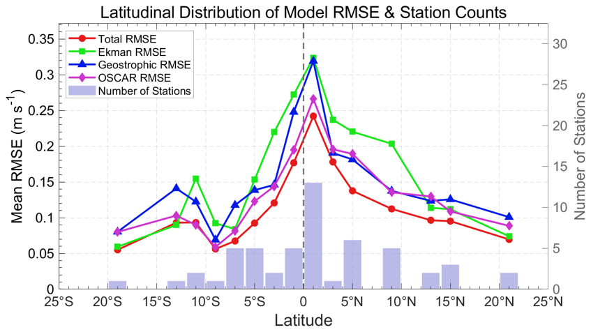
Figure 4 The latitudinal error curves of the in situ measurements against both the corresponding AC-PIDNN corrected currents and the OSCAR products across the 54 observation stations.

The Root Mean Square Error (RMSE) was utilized to evaluate the AC-PIDNN-corrected total currents, OSCAR currents, geostrophic currents (Geo), and Ekman corrected currents (Fig. 3b–d). Statistical results demonstrate that across all three major ocean basins, the surface circulations corrected by AC-PIDNN are significantly closer to the in situ observations compared to the traditional geostrophic and Ekman corrected components. Specifically, in the Pacific Ocean, the RMSE of the AC-PIDNN-corrected current is 0.16 m s⁻¹, which outperforms the Ekman corrected (0.24 m s⁻¹), geostrophic (0.22 m s⁻¹), and standard OSCAR product (0.19 m s⁻¹) currents, achieving an error reduction of approximately 15.8 % relative to OSCAR. In the Indian Ocean, the RMSE of AC-PIDNN is 0.10 m s⁻¹, outperforming both the Ekman corrected (0.13 m s⁻¹) and geostrophic (0.15 m s⁻¹) currents, with a 23.1 % error reduction compared to OSCAR (0.13 m s⁻¹). In the Atlantic Ocean, the RMSE of AC-PIDNN is 0.15 m s⁻¹, which is lower than the Ekman corrected (0.22 m s⁻¹) and geostrophic (0.17 m s⁻¹) currents, representing an 11.8 % error reduction compared to OSCAR (0.17 m s⁻¹). Furthermore, the Supplement provides time-series comparisons of the measured currents against the AC-PIDNN corrected flow fields, OSCAR products, as well as the geostrophic and Ekman corrected components at 16 stations. Please refer to Figs. S3–S6.

It is important to note that because these 54 independent stations from the TAO, PIRATA, and RAMA arrays are confined to the tropical regions (roughly ± 25° of the equator), this in situ validation is inherently biased toward regimes where advective and Ekman effects are large relative to the geostrophic flow. Therefore, while the validation demonstrates that the AC-PIDNN dataset delivers consistent and good agreement with the available mooring observations across the tropical Pacific, Atlantic, and Indian Oceans, the performance of the dataset in other regions requires further validation with additional in situ measurements.

To further evaluate the spatial distribution characteristics of the errors, a latitudinal error analysis of the AC-PIDNN and OSCAR surface current products was conducted using the in situ observations. As illustrated in Fig. 4, within the latitudinal range of approximately ± 25° (corresponding to the spatial coverage of the deployed observation arrays), the AC-PIDNN-corrected dataset consistently outperforms the OSCAR product in matching the in situ measurements. The analysis reveals that larger errors are predominantly concentrated in the equatorial band (within a latitude range of approximately ± 5°). Conversely, accuracy improves significantly in mid-to-low latitudes and regions further from the equator, aligning much more closely with field observations. Specifically, the RMSE decreases gradually from 0.25 m s⁻¹ near the equator to 0.05 m s⁻¹ in the higher-latitude observation areas. Overall, within the ± 25° latitudinal band, the AC-PIDNN product consistently demonstrates better performance than the OSCAR product, indicating that the improved reliability of the dataset is not an isolated artifact but a geographically consistent feature across a broad spatial extent. Additionally, it should be noted that due to the limited spatial coverage of current continuous in situ observation arrays, there is presently a lack of robust mooring data in high-latitude regions (e.g., the poles) for further validation.

4.1.3 Comparison of AC-PIDNN corrected flow fields against ROMS data

To further evaluate the reconstruction accuracy, we conducted an additional validation using a high-resolution ROMS simulation as a supplementary reference. The simulation results were not involved in training but were used mainly as an additional source of evidence to further assess the effectiveness of the proposed method. In this experiment, the ROMS simulated sea surface height was used as the sole input to reconstruct the surface velocity field, ensuring a fair comparison between the baseline iterative method and the AC-PIDNN approach. As the ROMS simulation used herein neglects the Ekman component, this component is not taken into account in the present study. Figure 5 compares the reconstructed surface velocity fields with the ROMS reference in the northwestern Pacific Ocean. The zonal (u) and meridional (v) velocity components, as well as the velocity magnitude, are shown for the ROMS simulation, the Iteration method, and the AC-PIDNN reconstruction. The Iteration method reproduces the general structure of the velocity fields but exhibits substantial amplitude mismatches, particularly in regions of strong currents and mesoscale activity, with RMSE values of 0.12 m s⁻¹ for u, 0.16 m s⁻¹ for v, and 0.11 m s⁻¹ for the magnitude of the velocity over the mapped domain. In contrast, the AC-PIDNN reconstruction reproduces the dominant spatial structures of the surface circulation more faithfully. The pathway and intensity of the western boundary current, as well as the surrounding mesoscale features, are captured with improved spatial coherence. Correspondingly, the RMSE is reduced to approximately 0.01 m s⁻¹ for both velocity components and for the velocity magnitude, representing nearly an order of magnitude improvement over the iterative approach. Together with the momentum balance diagnostics, the ROMS based validation confirms that the corrected surface circulation is both dynamically consistent and quantitatively accurate under controlled conditions.

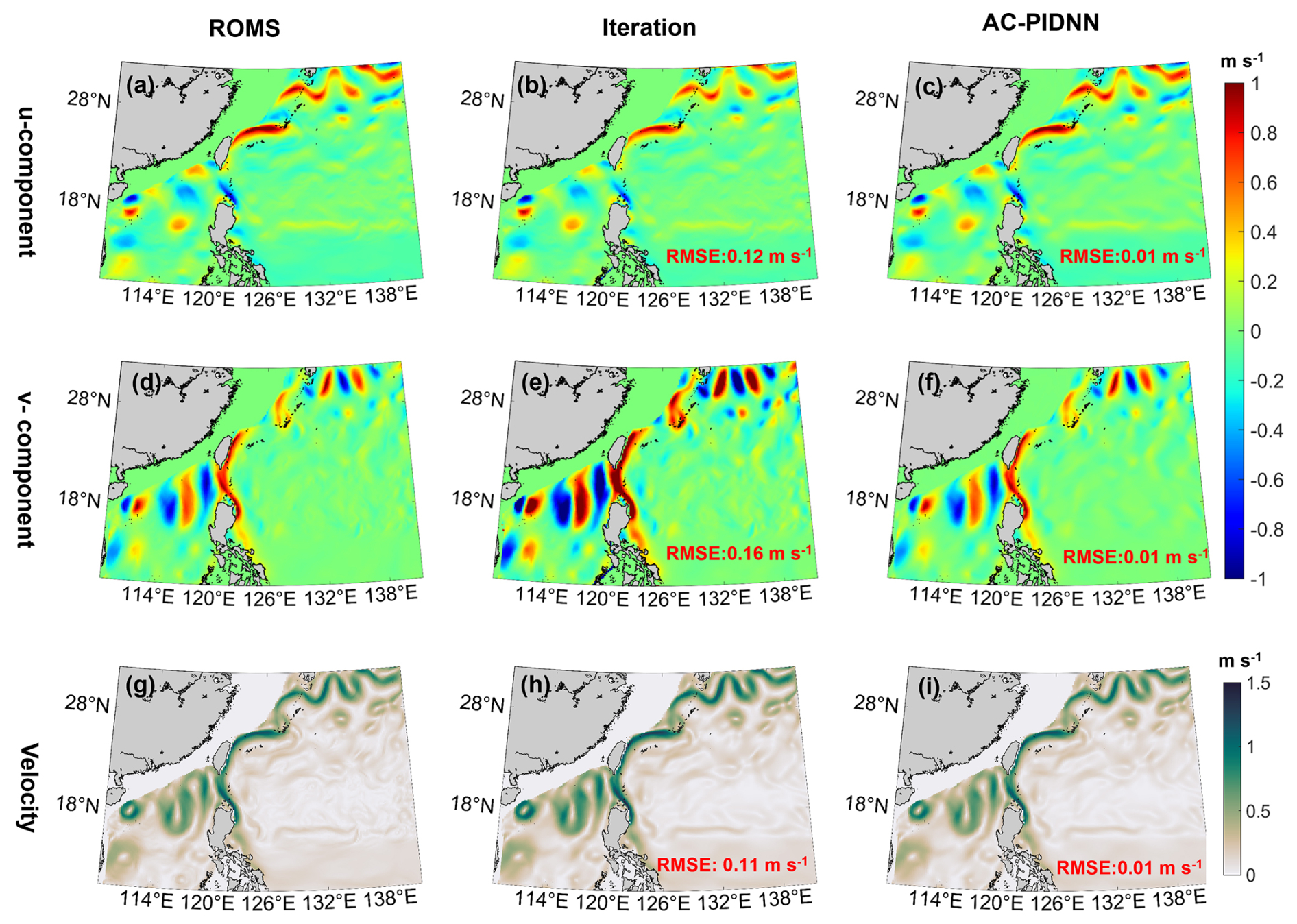
Figure 5 Sea surface flow field after correction of sea surface height anomalies in the Northwestern Pacific using iterative method and AC-PIDNN. The first column shows the u-component, v-component, and flow field of the simulated data; the second column show the results corrected by the iterative method and AC-PIDNN method.

4.2 Characteristics of the corrected surface circulation

In this section, we decompose the daily surface circulation (1993–2023) into geostrophic (V_geo), Ekman corrected (V_Ekman), nonlinear advective (V_adv) components. The detailed results for the Kuroshio region and the equatorial Pacific region are shown in Figs. S8 and S9, respectively. For each component, we analysed the zonal and meridional velocity components (u and v) together with the flow speed (Fig. 6).

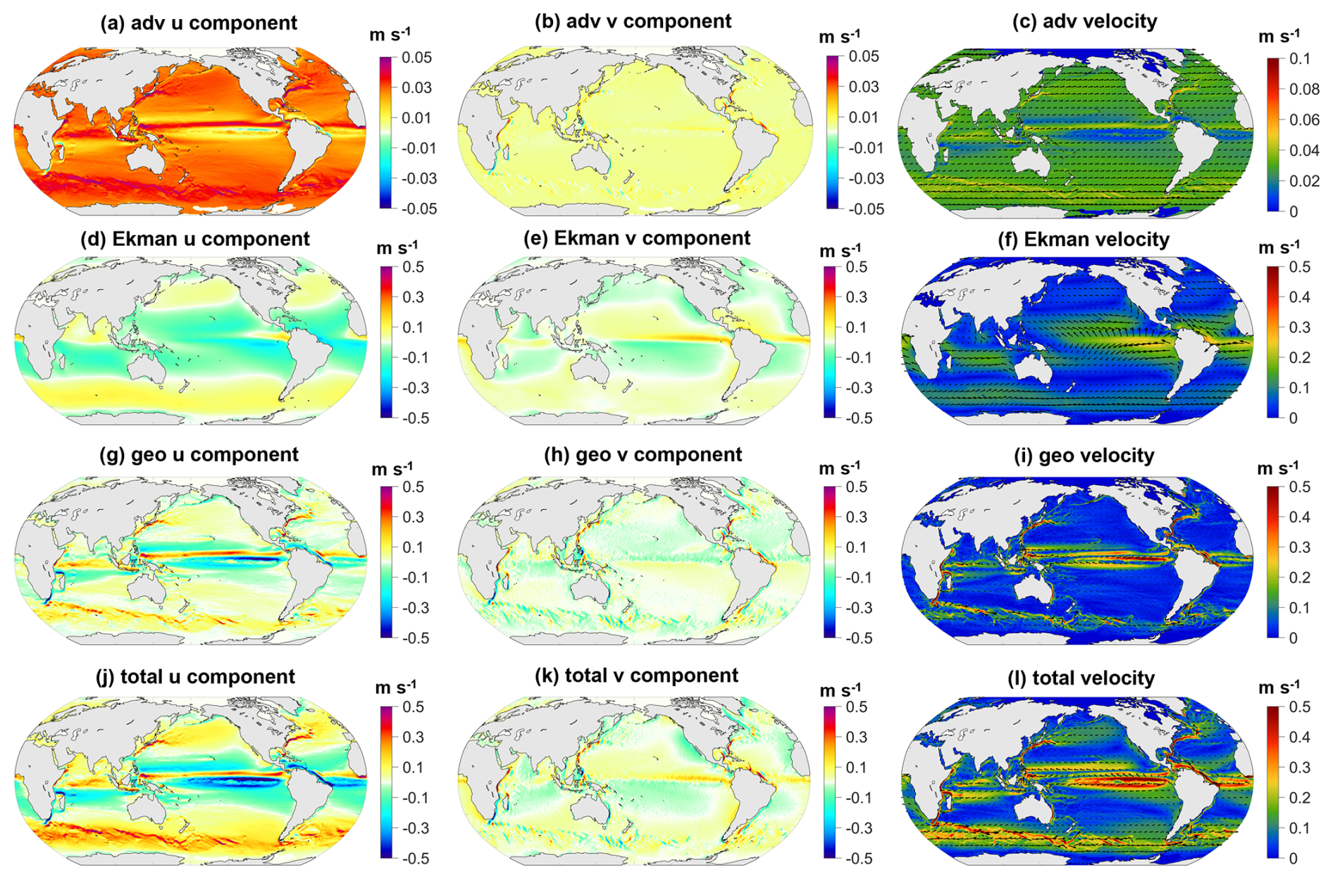
Figure 6 Results of sea surface circulation correction from 1993 to 2023, using the AC-PIDNN model, incorporating geostrophic, nonlinear advective and Ekman corrected components. Panels (a)–(c) show the u-component, v-component, and flow field of the nonlinear advective component; (d)–(f) show the u-component, v-component, and flow field of the Ekman corrected component; (g)–(i) show the u-component, v-component, and flow field of the geostrophic component; (j)–(l) show the u-component, v-component, and flow field of the total circulation.

The nonlinear advective component (Fig. 6a–c) exhibits a relatively smaller magnitude. Both its zonal and meridional contributions are generally on the order of 10⁻² m s⁻¹, with elevated values confined to dynamically active regions. These localized enhancements are most evident along the equatorial band, within western boundary current systems and their extensions, and over parts of the Southern Ocean (Qiu et al., 2014). Over the majority of the open ocean, the advective component remains weak, indicating that its contribution to the corrected surface circulation is primarily expressed through regional and localized modulation rather than basin-scale influence. The Ekman corrected component (Fig. 6d–f) displays a clear large-scale organization. Its zonal and meridional velocities show pronounced latitudinal banding over wide areas of the tropics and subtropics, consistent with the distribution of large-scale wind forcing. Typical Ekman corrected velocities reach O(10⁻¹) m s⁻¹ in low-latitude and mid-latitude regions, with reduced magnitudes toward higher latitudes.

The large-scale structure and intensity of the surface circulation are primarily controlled by the geostrophic flow (Fig. 6g–i). Both zonal and meridional geostrophic velocities exhibit strong signals associated with major current systems, including western boundary currents and their extensions and the Antarctic Circumpolar Current. The geostrophic speed commonly reaches O(10⁻¹–10⁰) m s⁻¹. The weaker values are found in the interiors of subtropical gyres. As a result of the combined contributions, the total surface velocity field (Fig. 6j–l) closely resembles the geostrophic circulation in its overall structure, while exhibiting systematic modifications in both magnitude and spatial details. In particular, westward zonal flow near the equator and Southern Ocean, and meridional transport in adjacent regions are strengthened relative to a purely geostrophic approximation, highlighting the cumulative influence of Ekman corrected and nonlinear advective processes in shaping the corrected surface circulation. Neglecting these ageostrophic components would therefore bias the spatial distribution and magnitude of reconstructed surface currents.

Because the total velocity is defined as the linear sum of the three components, this decomposition provides a natural basis for examining their respective contributions to commonly used kinematic and energetic diagnostics, as discussed in the following section.

4.3 Impacts on kinematic and energetic diagnostics

This section examines the impacts of the velocity correction on commonly used kinematic and energetic diagnostics, including surface relative vorticity (VOR), divergence (DIV), and eddy kinetic energy (EKE). These variables are widely applied in studies of upper ocean dynamics (Wunsch, 2025) and therefore provide an important perspective on the implications of the corrected surface circulation.

$$\begin{array}{}\text{(19)}& {\displaystyle }\text{VOR}={\displaystyle \frac{\partial v}{\partial x}}-{\displaystyle \frac{\partial u}{\partial y}}\text{(20)}& {\displaystyle }\text{DIV}={\displaystyle \frac{\partial u}{\partial x}}+{\displaystyle \frac{\partial v}{\partial y}}\text{(21)}& {\displaystyle }\text{EKE}={\displaystyle \frac{\mathrm{1}}{\mathrm{2}}}(u^{\prime \mathrm{2}}+v^{\prime \mathrm{2}})\end{array}$$

4.3.1 Vorticity

Sea surface relative vorticity is a key dynamical parameter that describes the rotational characteristics of the upper ocean flow, directly linked to flow shear, vortex structures, and angular momentum distribution (Zhang et al., 2024; Kwak and Richmond, 2014). The geostrophic component (Fig. 7c) dominates the large-scale structure of the relative vorticity field. Regions of strong positive and negative vorticity are closely aligned with major current systems, including western boundary currents, their downstream extensions, and the Antarctic Circumpolar Current. This distribution outlines the primary rotational framework of the surface circulation and reflects the strong shear associated with geostrophic jets and frontal zones. In addition to the geostrophic component, the wind-driven Ekman flow contributes significantly to the sea surface relative vorticity. Here, the Ekman corrected component refers specifically to the vorticity generated by the velocity field that balances the wind stress forcing in the horizontal momentum equations (i.e., the Ekman flow), as distinct from the vertical Ekman pumping velocity associated with wind stress curl (Chen et al., 2020). While generally weaker in magnitude than geostrophic vorticity, this component exhibits distinct regional signatures. Enhanced Ekman vorticity (Fig. 7b) is particularly evident in tropical and subtropical basins where winds are strong and relatively steady, such as the trade wind belts and prevailing westerlies, where lateral shear in the Ekman corrected velocity can generate significant vorticity signals (Chen et al., 2020). For instance, in equatorial regions, zonal wind stress can excite pronounced Ekman vorticity anomalies due to the variation of the Coriolis parameter. In contrast, the nonlinear vorticity (Fig. 7a) term arising from advection by the flow itself is typically about two orders of magnitude smaller in strength than the geostrophic and -corrected components. However, in regions of intense currents and strong shear, such as the Kuroshio Extension and Gulf Stream separation zones, nonlinear processes become crucial in modulating vorticity variability, energy cascade, and submesoscale vortex activities, and thus cannot be neglected(Chen et al., 2020). We present the 30-year average vorticity for the western boundary Kuroshio region and the wind forced equatorial Pacific current region in Figs. S10a–d and S11a–d, respectively. This indicates that while the foundational structure of the large-scale vorticity field is set by geostrophic balance, with wind forcing and nonlinear dynamics providing an additional contribution to vorticity magnitude particularly in dynamically active regions.

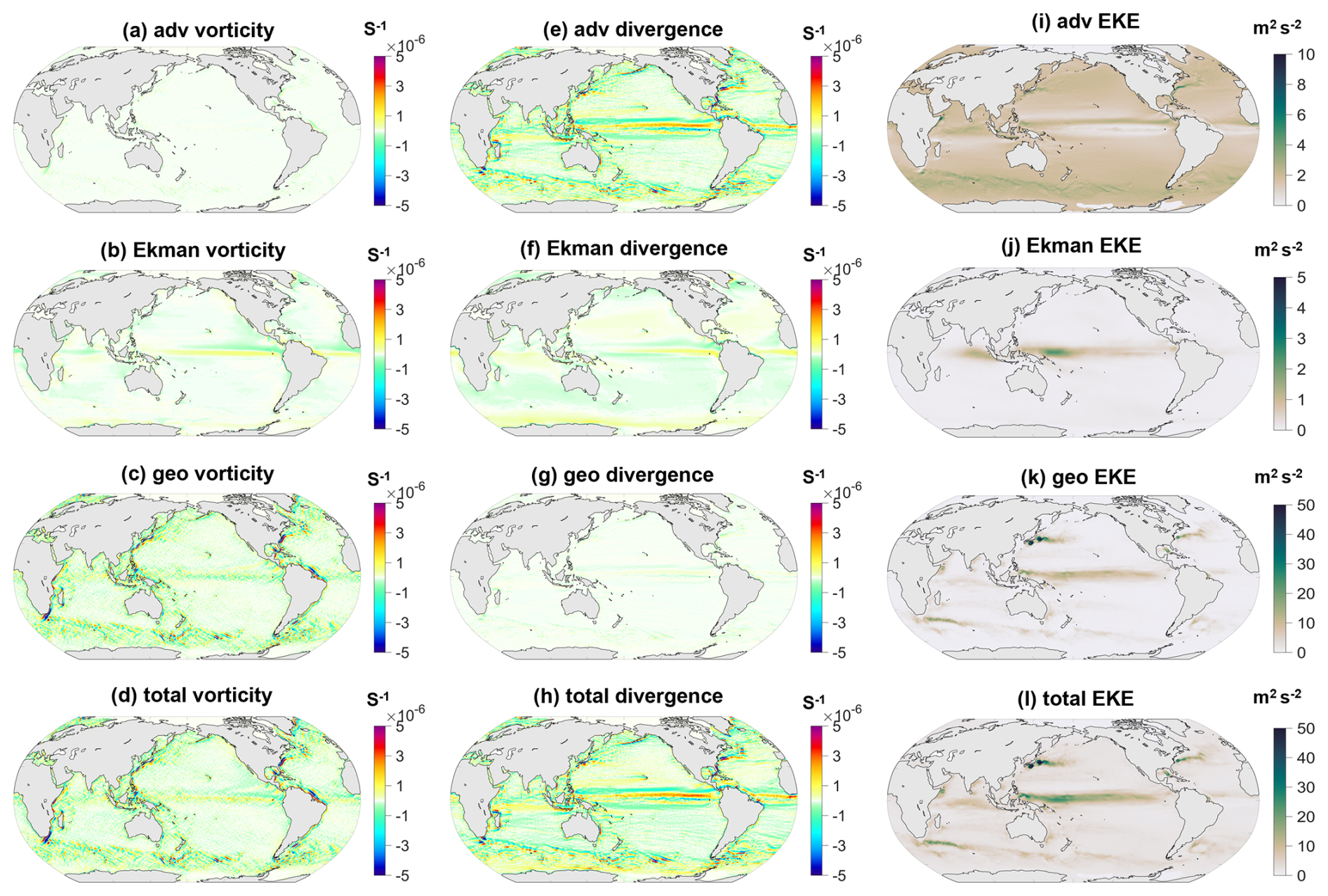
Figure 7 30-year average global sea surface dynamic parameter characteristics. Panels (a)–(d) showing the vorticity of the advective, Ekman corrected, geostrophic, and total components, respectively; (e)–(h) showing the divergence of the advective, Ekman corrected, geostrophic, and total components, respectively; (i)–(l) showing the EKE of the advective, Ekman corrected, geostrophic, and total components, respectively.

4.3.2 Divergence

Sea surface horizontal divergence is a key physical quantity characterizing the divergent/convergent nature of the upper-ocean flow, with important implications for mass transport (Dubois et al., 2016). Unlike the vorticity field, the dynamical components of the divergence field exhibit distinct and contrasting contributions. From a dynamical decomposition perspective, the horizontal divergence of the geostrophic component (Fig. 7g) is negligible at the sea surface under the continuum layer approximation, dictated by its non-divergent nature. Thus, the geostrophic flow contributes insignificantly to the large scale sea surface horizontal divergence. In contrast, the nonlinear advective component (Fig. 7e) dominates the large-scale spatial pattern of the divergence field. Its magnitude is substantially larger than other components, forming prominent bands of divergence/convergence in regions of strong currents (e.g., western boundary current extensions) and vigorous eddy activity. It is noteworthy that although the local amplitude of the advective divergence is large, its net contribution to basin scale or global integrated divergence is modest due to the cancellation between extensive positive and negative regions. The Ekman corrected component of divergence (Fig. 7f), however, originates directly from Ekman pumping/suction driven by wind stress curl. Its local intensity is typically weaker than the advective component. Due to its more spatially coherent sign (e.g., divergence over regions of positive wind stress curl and convergence over negative curl regions), the Ekman corrected component contributes significantly to the domain averaged or net divergent effect at regional or global scales, and its magnitude is non-negligible. For instance, in the major wind belts (trade winds, westerlies), Ekman divergence forms a key driver for large-scale vertical circulation cells, such as the subtropical gyres (Roquet et al., 2025). To further illustrate the impacts of nonlinear processes and wind forcing on sea surface divergence, we present the 30-year average vorticity for the western boundary Kuroshio region and the wind-forced equatorial Pacific current region in Figs. S10e–h and S11e–h, respectively.

4.3.3 Eddy Kinetic Energy

EKE is an integrated metric for the intensity of mesoscale variability, representing the perturbation energy of the flow velocity field relative to its temporal mean. It serves as a key parameter for assessing the energetic consistency and dynamical plausibility of the corrected velocity field (Huo et al., 2024). As shown in Fig. 7i–l the global EKE distribution derived from the corrected circulation field, which incorporates geostrophic, Ekman corrected, and nonlinear advective components exhibits the well documented pattern of high energy regimes: primarily concentrated in western boundary current extensions (e.g., the Kuroshio Extension, Gulf Stream Extension), the core regions of the Antarctic Circumpolar Current, and equatorial current systems, all areas of high dynamical activity (Su et al., 2023). To further illustrate this point, Figs. S10i–l and S11i–l present the 30-year mean EKE characteristics in the equatorial Pacific region and the Kuroshio region, respectively. These energetic hotspots are closely linked to strong shear, instability processes, and active mesoscale eddy generation. Compared to EKE estimates based solely on the geostrophic approximation, the inclusion of the Ekman and nonlinear advective components does not introduce spurious amplification of the total kinetic energy. Instead, it redistributes the energy spatially in a physically consistent manner. The correction primarily modulates the structure of the EKE field rather than significantly altering its global intensity magnitude. Specifically, in regions where wind forcing is pronounced, such as the equatorial and subtropical zones, incorporating the Ekman corrected component provides a more realistic representation of fluctuating energy directly generated by wind variability. Meanwhile, in the vicinity of strong current edges and frontal zones, nonlinear advective processes dominate in shaping the fine scale structure of EKE, such as energy cascade and eddy-mean flow interactions (Adeagbo et al., 2022). In summary, the multi-component velocity correction scheme redistributes the spatial pattern of EKE in a manner consistent with physical mechanisms while preserving the overall energetic framework of the surface circulation. This enhances the capability of the EKE field to characterize mesoscale processes, energy transfer pathways, and mixing efficiency, yielding a representation that is closer to the true dynamical context of the ocean.

4.3.4 Temporal evolution of dynamical diagnostics

To analyze the long-term variations in the three dynamic parameters mentioned above, Fig. 8 presents the 30-year averaged time series for the global ocean, the Kuroshio region (110–175° E, 12–50° N), and the Equatorial Current region (60° W–110° E, 20° S–20° N). On a global scale (Fig. 8a–c), the interannual variability of total divergence (O(10⁻⁸) s⁻¹) is primarily dominated by the Ekman corrected component (O(10⁻⁹) s⁻¹), with the nonlinear component (O(10⁻⁹) s⁻¹) also contributing significantly, and their variation trends are largely consistent. The magnitude of variability in nonlinear divergence is smaller than that of the Ekman corrected component but significantly larger than the negligible geostrophic divergence (O(10⁻¹⁰) s⁻¹). The total relative vorticity field (O(10⁻⁹) s⁻¹) is mainly determined by the combined effects of the geostrophic component (O(10⁻⁹) s⁻¹) and the Ekman corrected component (O(10⁻¹⁰) s⁻¹). In terms of trends, the Ekman corrected vorticity exhibits a weakening trend, whereas both geostrophic and total vorticities show a long-term enhancement of negative vorticity. No significant interannual signal is detected in nonlinear vorticity. Regarding EKE, the trend in total EKE aligns with that of geostrophic EKE but is notably modulated by nonlinear processes. Moreover, the magnitudes of the nonlinear and geostrophic components are comparable, with the nonlinear EKE being higher in most years, yet both remain within the same order of magnitude (O(10⁰–10¹) m² s⁻²).

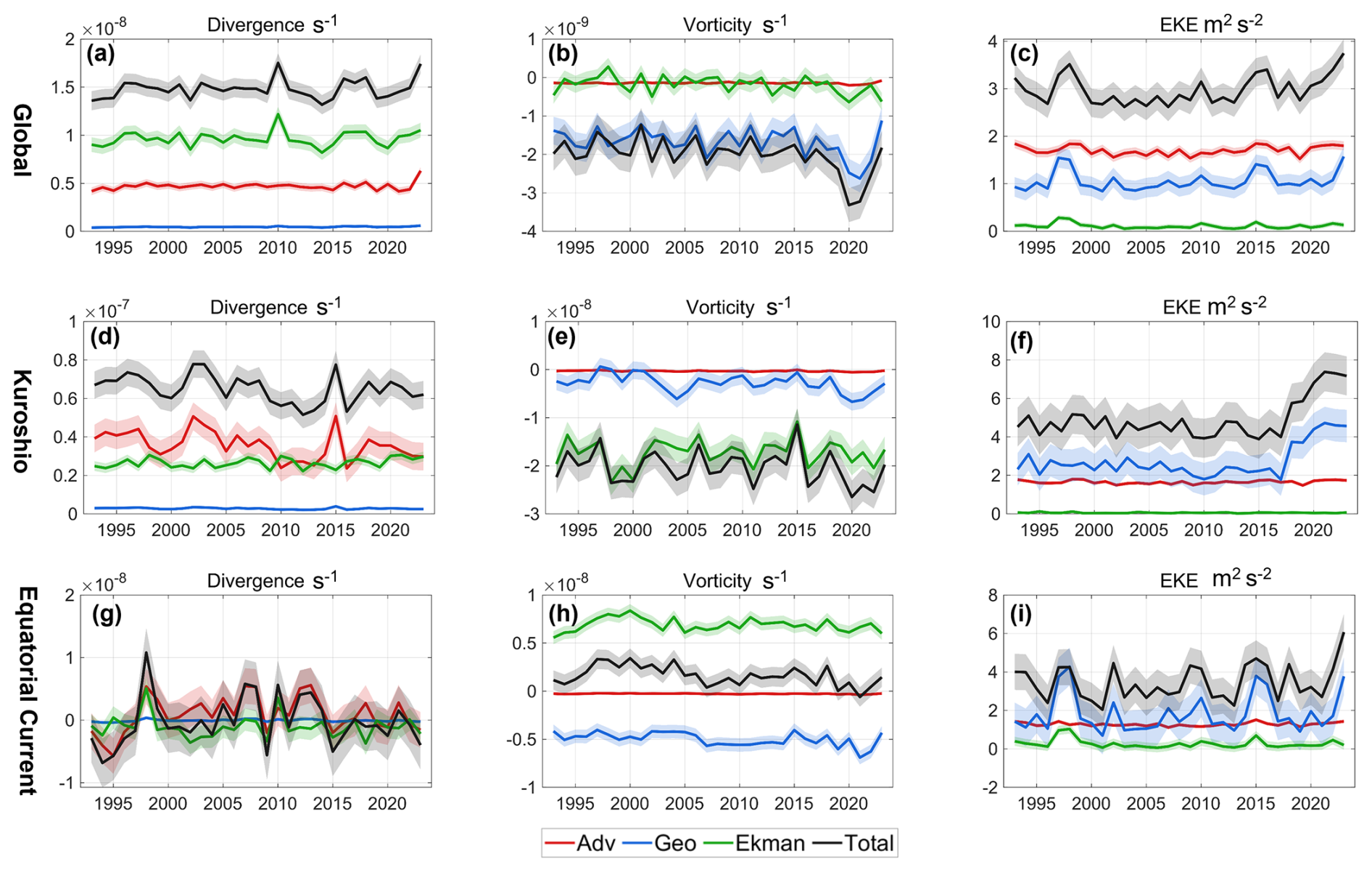
Figure 8 The annual mean variations in sea surface divergence, vorticity, and EKE from 1993 to 2023 for the global ocean, the Kuroshio region, and the equatorial current region. Panels (a)–(c) illustrate the interannual changes in globally averaged sea surface divergence, vorticity, and EKE; (d)–(f) show the corresponding variations in the Kuroshio region (110–175° E, 12–50° N); and (g)–(i) display the changes in the equatorial current region (110–175° E, 12–50° N). The shaded area around each curve represents the ± 1 standard deviation range.

Table 1 Dataset Variable Information.

On a regional scale, two representative areas, the Kuroshio region and the Equatorial Current region are selected for analysis (Fig. 8d–i). In the Kuroshio region, the variation in total divergence follows the trend of the nonlinear component, although the contribution of the Ekman corrected component is non-negligible, particularly in equatorial areas. The magnitude of divergence in the Kuroshio region (O(10⁻⁸) s⁻¹) is larger than that in the Equatorial Current region (O(10⁻⁹) s⁻¹). Regarding vorticity, the Kuroshio region is dominated by negative vorticity, with the absolute value of the Ekman corrected component being significantly larger than that of the geostrophic component. In contrast, the Equatorial Current region exhibits positive Ekman corrected vorticity and negative geostrophic vorticity, with total vorticity primarily contributed by the Ekman corrected component. Additionally, the magnitudes of geostrophic and total vorticities in the Kuroshio region (O(10⁻⁸) s⁻¹) exceed those in the Equatorial Current region (O(10⁻⁹) s⁻¹). For EKE, variations in both regions are mainly governed by the geostrophic component. The trend in total EKE in the Equatorial Current region closely resembles that of its geostrophic component, whereas the Kuroshio region has shown an increasing trend in EKE since approximately 2017. In terms of magnitude, total EKE, geostrophic EKE, and nonlinear EKE are all on the order of O(10⁰–10¹) m² s⁻². The Ekman corrected EKE in the Equatorial Current region (O(10⁻¹) m² s⁻²) is larger than that in the Kuroshio region (O(10⁻²) m² s⁻²).

5 Code and data availability

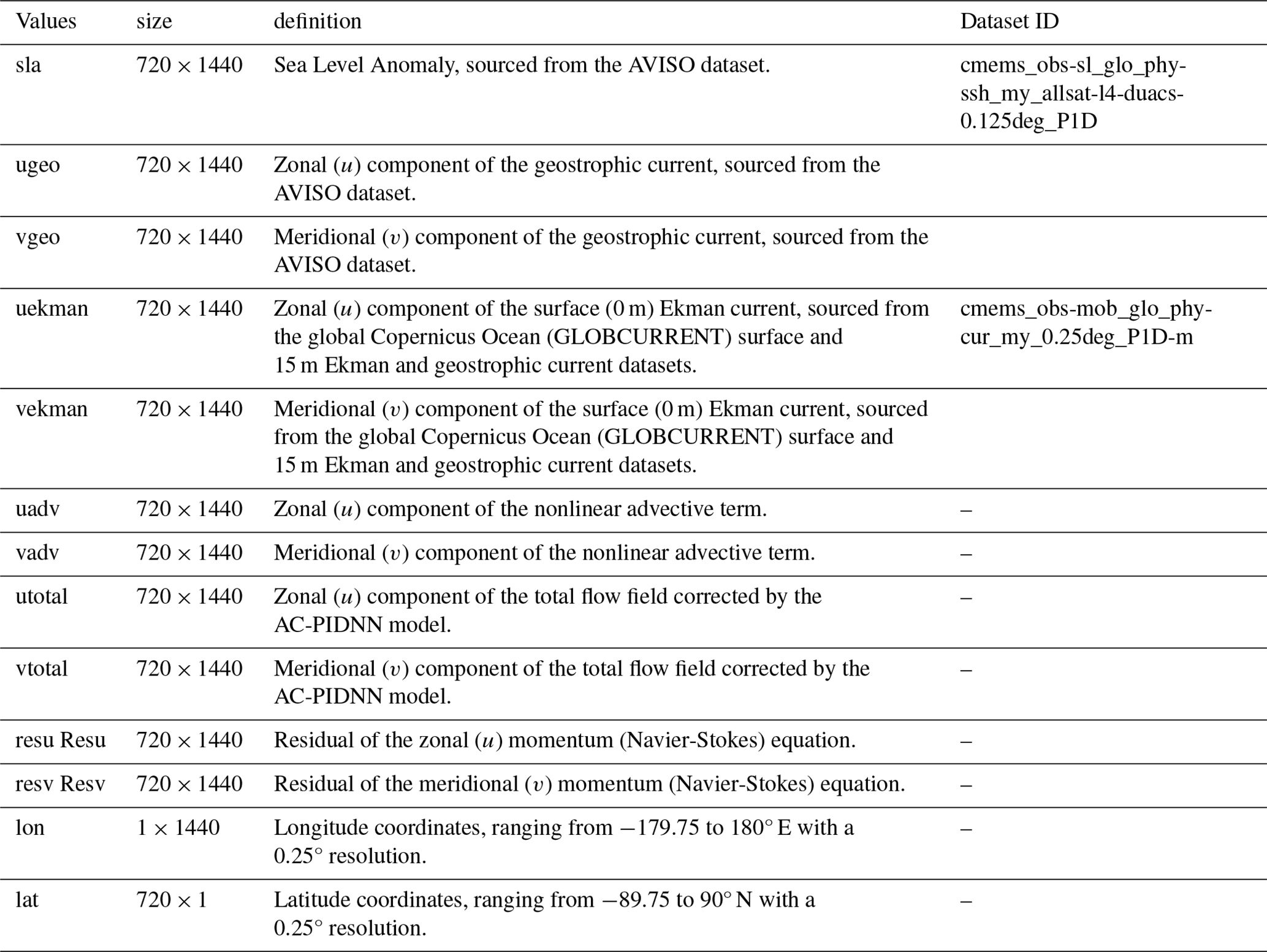
The code for AC-PIDNN is available at https://doi.org/10.5281/zenodo.23901902 (Cui, 2026). The global sea surface circulation dataset corrected for the period 1993–2023 in this study can be accessed via https://doi.org/10.5281/zenodo.19966716 (Cui and Cai, 2026). This dataset has a spatial resolution of 0.25°, and each daily flow field file contains the variable names and their descriptions as listed in Table 1. Furthermore, the table outlines the Dataset ID corresponding to the satellite data product (global gridded geostrophic currents and surface Ekman currents) obtained from the Copernicus Marine Service at: https://data.marine.copernicus.eu/product (last access: 3 November 2026).

6 Conclusions

A key contribution of this study is the development of a physics-informed deep learning framework to correct sea surface currents and quantify their dynamical components. By explicitly incorporating physical constraints, the framework substantially improves the dynamical consistency of reconstructed surface circulation and yields a global daily dataset for 1993–2023. Our results show that, although ageostrophic components are generally smaller than the geostrophic flow, they make important contributions to the total surface circulation, especially in energetic regions such as western boundary currents and the Kuroshio Extension. On a global scale, the mean velocity of the total flow field is on the order of $\mathit{O}\left({\mathrm{10}}^{-\mathrm{2}}\text{–}{\mathrm{10}}^{-\mathrm{1}}\right)$ m s⁻¹, with the Ekman corrected, geostrophic, and nonlinear components each exhibiting magnitudes of O(10⁻²) m s⁻¹. In particular, nonlinear contributions have limited influence on relative vorticity, as the dominant rotational structure is captured by the geostrophic circulation. In contrast, the nonlinear corrections strongly affect surface divergence and eddy kinetic energy, revealing aspects of ocean surface dynamics that are not captured by geostrophic circulation alone. These findings show that resolving ageostrophic dynamics is essential for a more complete understanding of global surface circulation and its variability.