MLAWind: a monthly sea surface wind dataset derived from an interpretable machine learning approach integrating in-situ observations and satellite data

A gridded sea surface wind dataset with long temporal coverage is crucial for understanding atmospheric circulation changes and air–sea interactions at different time scales. This study employs an interpretable machine learning model based on random forest algorithm to generate a 1° × 1° monthly sea surface wind dataset (MLAWind) from 1950 to 2023, covering the near-global ocean within 60° S–60° N. The data reconstruction model integrates the Cross-Calibrated Multi-Platform (CCMP) satellite data and the spatially sparse long-term International Comprehensive Ocean-Atmosphere Data Set (ICOADS), exhibiting robust interpretability and generalization capability. Quantitative validations against satellite and in-situ data indicate that MLAWind achieves better consistency with observations than most reanalysis datasets, maintaining robust performance during both training (1993–2022) and testing periods (2023). The performance of MLAWind since 1950 is assessed across multiple time scales. Its characteristics in climatology, annual cycle, and inter-annual variability are comparable to those of reanalysis datasets, even during the non-satellite period prior to 1993. Independent coral records from 1950–1982 are employed as proxy indicators to evaluate long-term sea surface wind trends. The trend derived from MLAWind is corroborated by these proxies, exhibiting significantly higher temporal correlation than those obtained from reanalysis products. MLAWind demonstrates a more reliable reconstruction of long-term sea surface wind variability during historical periods since 1950. The results indicate that MLAWind serves as a robust data resource for global climate change research. The reconstructed MLAWind dataset is publicly accessible at https://doi.org/10.12157/IOCAS.20250707.001 (Guo et al., 2025c).

1 Introduction

Sea surface wind is a critical factor in air–sea interactions, exerting significant impacts on climate change, marine ecosystem and human society (Tokinaga et al., 2012; Wang et al., 2018; Zhou et al., 2022). It governs variations of the hydrological cycle by modulating atmosphere-ocean heat and moisture exchanges (Held and Soden, 2006; Findell et al., 2019). Sea surface wind drives the large-scale redistribution of water masses and energy. The global ocean current systems, including the Kuroshio, Gulf Stream, South China Sea Throughflow, Indonesian Throughflow, and Antarctic Circumpolar Current, are primarily regulated by wind-driven Ekman transport and momentum transfer processes (Deser et al., 1999; Wang et al., 2006, 2023; Zhang et al., 2023b; Li et al., 2025). Sea surface wind can deliver energy to the deep ocean, inducing near-inertial waves and near-bottom currents (Zhang et al., 2024). Previous studies have demonstrated that equatorial sea surface wind anomalies are associated with the inter-annual variability of the tropical sea surface temperature (SST) anomalies, which promotes the development of El Niño-Southern Oscillation (ENSO) events (Kug, et al., 2009; Clarke, 2014; Wang, 2019). Sea surface wind is thus utilized as a precursor to improve the predictability of different types of ENSO (Ren et al., 2019; Tseng et al., 2022).

The existing observational sea surface wind datasets exhibit notable limitations despite remarkable advances in observation platforms and sensor technologies. Satellite data are characterized by exceptional spatiotemporal continuity, offering a robust data foundation for retrieving climate system characteristics at the global scale, including those associated with extreme meteorological events (Vinoth and Young, 2011; Yang et al., 2015; Young and Ribal, 2019). However, the relatively short temporal coverage of satellite observations constrains their capacity to analyze climate variability from inter-decadal time scale to long-term trends. The International Comprehensive Ocean-Atmosphere Data Set (ICOADS) is widely acknowledged as the most extensive and comprehensive global surface ocean dataset. It provides in-situ observations of critical atmospheric and oceanic variables dating back to 1662 (Freeman et al., 2017). In contrast to the extensive spatial coverage of satellite data, ICOADS exhibit an irregular distribution and suffer from significant sampling errors. Due to these deficiencies in existing observational datasets, the Sixth Assessment Report by the Intergovernmental Panel on Climate Change (IPCC AR6) assigns a 'low to medium' confidence level for the historical sea surface wind trends assessment (IPCC, 2023).

A long-term gridded global wind dataset can be constructed by integrating in-situ and satellite observations. Numerous reanalysis products have assimilated the ICOADS data and multi-platform satellite observations through data assimilation techniques, significantly extending the temporal-spatial coverage of the sea surface wind field (e.g. Kalnay et al., 1996; Kobayashi et al.,2015; Hersbach et al., 2019). The inherent limitations of reanalysis datasets primarily stem from two aspects: (1) the assimilation methodologies and models introduce significant biases into the reanalysis products; (2) variations in the types and volumes of in-situ data result in sampling biases. Substantial uncertainties persist in reanalysis datasets with different assimilation methodologies and data sources (Zhang et al., 2023a).

In addition to data assimilation techniques, direct reconstruction methods based on ICOADS data are employed in some studies (Berry and Kent, 2011; Tokinaga and Xie, 2011; Tokinaga et al., 2012). For example, the Wave- and Anemometer-Based Sea Surface Wind (WASWind) achieves high accuracy by integrating anemometer-measured winds and wave height-estimated winds from the ICOADS data (Tokinaga and Xie, 2011). WASWind exhibits a relatively coarse spatial resolution of 4° × 4° and limited temporal coverage from 1950 to 2008. The National Oceanography Centre Southampton Flux Dataset v2.0 (NOCS2) is another reconstructed dataset derived from the ICOADS data. It features an enhanced spatial resolution of 1° × 1° but covers a shorter time period (1973–2014) for sea surface wind speed (Berry and Kent, 2011).

Machine learning algorithms demonstrate superior capability in capturing nonlinear relationships between different variables compared to traditional techniques (Reichstein et al., 2019; Jiang et al., 2024; Wang and Li, 2024, He et al., 2026). These algorithms are applied in the reconstruction of various datasets such as sea surface temperature (Huang et al., 2025), air temperature (Yoo et al., 2018; He et al., 2022), ocean salinity (Tian et al., 2022), ocean heat content (Su et al., 2020; Bagnell and DeVries, 2021), carbon and water fluxes (Leng et al., 2024), and terrestrial water storage (Yin et al., 2023). Traditional machine learning models suffer from interpretability challenges, as their input-output mappings are treated as “black-box” systems lacking physically meaningful explanations. Recently, resolving machine learning interpretability issues has emerged as a critical research priority (Tian et al., 2022; Qin et al., 2024). SHapley Additive exPlanations (SHAP) is a reliable interpretable module based on cooperative game theory, which demonstrates excellent compatibility across diverse machine learning models (Lundberg and Lee, 2017; Kim et al., 2025). By generating both global and local interpretability, SHAP enables a more comprehensive attribution analysis than conventional feature importance metrics. The continuous advancement of interpretable machine learning techniques offers a robust methodology for historical sea surface wind reconstruction.

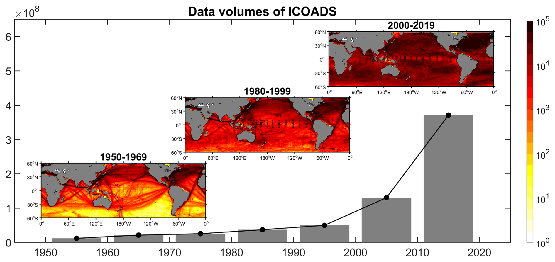
Figure 1 The volumes of ICOADS dataset since 1950. The bar illustrates the decadal cumulative volume of ICOADS dataset. The spatial distributions of the volumes of ICOADS dataset are presented in different periods.

This study employs an interpretable machine learning algorithm (Tian et al., 2022; Kim et al., 2025) to integrate ICOADS and satellite data, constructing a 1° × 1° monthly sea surface wind dataset from 1950–2023 with near-global ocean coverage within 60° S–60° N. The rest of the paper is organized as follows: the datasets, methods and data reconstruction model used in this study are described in Sect. 2; the evaluation processes of the reconstructed dataset are shown in Sect. 3; the performances of the reconstructed dataset at different time scales are examined in Sect. 4; the data availability statement is provided in Sect. 5; the study is summarized in Sect. 6.

2 Data and methods

2.1 Input data for model establishment

The reconstructed dataset is derived from in-situ observations of the ICOADS dataset. The ICOADS dataset provides an extensive collection of observations from diverse observing systems, containing multiple essential atmospheric and oceanic variables (Freeman et al., 2017). The incorporation of physically relevant feature inputs significantly enhances the reconstruction accuracy of machine learning models (Tian et al., 2022; Zhang et al., 2022). Multiple variables closely associated with sea surface winds are utilized in this study, including sea surface wind speed (WS), wind direction (WD), SST, air temperature (T_a), and sea level pressure (SLP) from 1950 to 2023. Note that the ICOADS observations exhibit pronounced spatiotemporal heterogeneity. During the period 1950–1969, data coverage is relatively limited in the Southern Hemisphere, contrasting with denser distributions in the North Pacific and North Atlantic Oceans. From 1980 to 1999, the data volume gradually increases, followed by significant growth after 2000, which achieves near-global coverage (Fig. 1).

Following previous studies (Berry and Kent, 2011; Tokinaga and Xie, 2011), comprehensive preprocessing is performed on the ICOADS dataset. All variables in the ICOADS dataset are subjected to rigorous quality control through an outlier detection procedure based on a climatological threshold of 3.5 standard deviations. The selection of the threshold aligns with the standardized processing implemented for both the ICOADS Monthly Summary Groups (MSG) product and the WASWind dataset (Tokinaga and Xie, 2011). Additional height adjustments are required for ICOADS sea surface winds, as the altitudes of ships and measurement instruments change over time. The bulk formulae and related parameters established by Smith (1980) are utilized to unify the unadjusted ICOADS sea surface winds to a standard reference height of 10 m. All data are initially processed into monthly means to enable point-to-point learning during model establishment process.

Table 1 A list of the datasets used in this study.

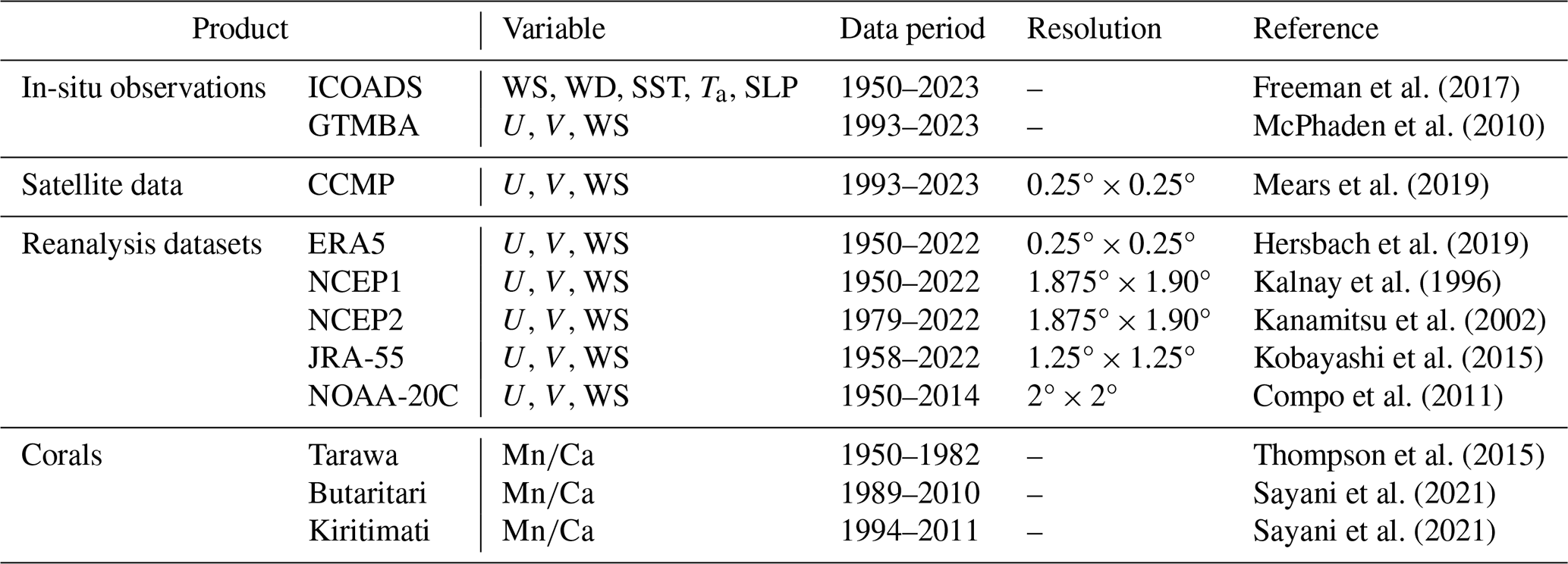
Satellite sea surface wind from the cross-calibrated multiplatform (CCMP) dataset is another important source of the reconstructed dataset. The CCMP dataset covers the period from 1993 to 2023 at a horizontal resolution of 0.25° × 0.25° (Mears et al., 2019). It is spatially interpolated onto a 1° × 1° grid to facilitate point-to-point learning with ICOADS dataset. The CCMP integrates multiple advanced satellites, including Advanced Scatterometer-A and B (ASCAT-A/B), Special Sensor Microwave/Imager (SSM/I), Special Sensor Microwave Imager/Sounder (SSMIS), Tropical Rainfall Measuring Mission's (TRMM) Microwave Imager (TMI), Global Precipitation Measurement (GPM) Microwave Imager (GMI), Advanced Microwave Scanning Radiometer-EOS (ASMR-E), Advanced Microwave Scanning Radiometer 2 (AMSR2), Quick Scaterometer (QuikScat), and Wind Satellite (WindSat). All satellite data are consistently converted to 10-m neutral stability winds, followed by inter-satellite cross-calibration to minimize systematic biases. Moored buoys are used to calibrate the satellite sensors, adjusting the CCMP background surface wind field during the data assimilation phase. Therefore, the CCMP demonstrates strong agreement with in-situ observations (Mears et al., 2019).

2.2 Data for evaluation

Five reanalysis products, including European Centre for Medium-Range Weather Forecasts (ERA5, Hersbach et al., 2019), the Japanese 55-year Reanalysis (JRA-55, Kobayashi et al., 2015), the National Oceanic and Atmospheric Administration 20th-Century Reanalysis (NOAA-20C, Compo et al., 2011), the National Centers for Environmental Prediction reanalysis 1 (NCEP1, Kalnay et al., 1996) and its upgraded version (NCEP2, Kanamitsu et al., 2002), are compared with the reconstructed dataset. All reanalysis products are spatially interpolated onto a 1° × 1° grid. Comprehensive descriptions of these datasets are presented in Table 1.

The Global Tropical Moored Buoy Array (GTMBA) in-situ observation is employed to evaluate the performance of multiple sea surface wind datasets. The GTMBA provides real-time observations in the tropics for weather and climate research. It integrates three buoy arrays, including the Tropical Atmosphere Ocean/Triangle Trans-Ocean Buoy Network (TAO/TRITON) in the Pacific Ocean, the Prediction and Research Moored Array in the Tropical Atlantic (PIRATA), and the Research Moored Array for African-Asian-Australian Monsoon Analysis and Prediction (RAMA) in the Indian Ocean (McPhaden et al., 2010). TAO provides a long-term observational record dating back to the early 1990s, while PIRATA and RAMA were deployed in 1997 and 2002, respectively. 56 TAO stations, 19 PIRATA stations, and 28 RAMA stations are utilized in this study.

Three coral $\mathrm{Mn}/\mathrm{Ca}$ records provided by Porites spp. corals are utilized to evaluate the long-term trends of sea surface wind. The coral record derived from Tarawa Atoll (1.33° N, 172.97° E) is resampled at approximately quarterly (4 per year) increments, spanning from 1894 to 1982 (Thompson et al., 2015). The coral records from Butaritari Atoll (3.07° N, 172.75° E) and Kiritimati Island (1.93° N, 157.49° W) exhibit bimonthly temporal resolution, covering the periods of 1989–2010 and 1994–2011, respectively (Sayani et al., 2021). These islands are located far from continental Mn sources and possess a west-facing lagoon that is sheltered from the easterly trade winds. Their $\mathrm{Mn}/\mathrm{Ca}$ records demonstrate a strong correlation with westerly wind events in the equatorial Pacific Ocean, serving as a valuable and independent resource for evaluating the zonal wind anomalies (Thompson et al., 2015; Sayani et al., 2021).

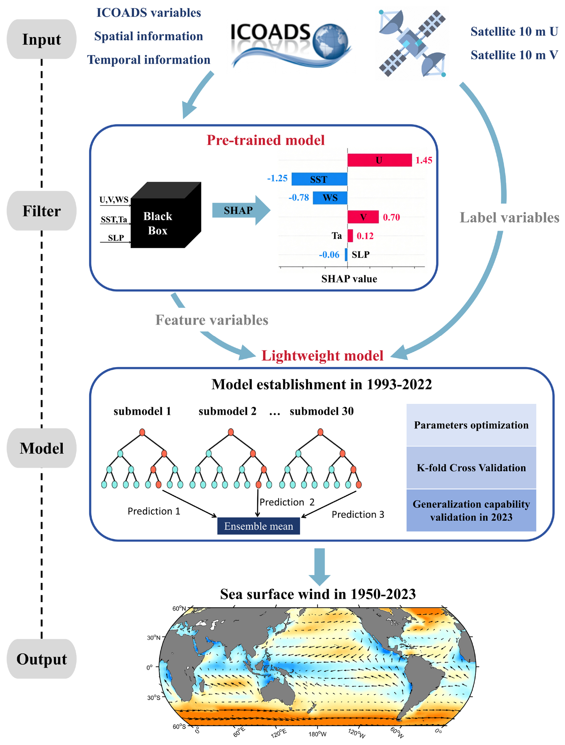
Figure 2 Schematic diagram of the construction process of machine learning-assisted sea surface wind dataset (MLAWind).

2.3 Data reconstruction model

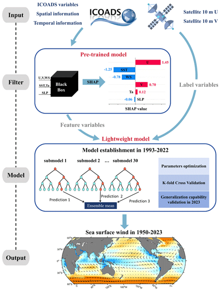
Figure 2 illustrates the schematic diagram of the construction process of the machine learning-assisted sea surface wind dataset (MLAWind). The random forest model is employed as the core algorithm. It effectively captures nonlinear relationships between feature and label variables through multiple decision trees (Breiman, 2001) and is extensively employed for temporal-spatial data processing (Yoo et al., 2018; Watt-Meyer et al., 2021; He et al., 2022). Notably, the inherent randomness in random forest model significantly improves its generalization capability, which is critical for robust reconstruction of long-term historical sea surface wind.

The reconstruction framework comprises four essential steps. The first is tokenization and preprocessing of the input data. Given that 10-m zonal wind, 10-m meridional wind and WS are routinely available from widely-used satellite and reanalysis products, these variables are selected as reconstruction targets to enable systematic inter-product comparison. Multiple ICOADS variables (WS, WD, SST, T_a, SLP) from 1993–2022 are used as feature inputs, while the CCMP 10-m wind field from 1993–2022 serves as the label variable for data reconstruction model establishment. The ICOADS data from 1950–1992 are employed in the model inference process to enable reconstruction of sea surface winds during historical periods without satellite data. All feature values for the data reconstruction model are normalized to enhance the efficiency of parameter optimization (Su et al., 2018; Watt-Meyer et al., 2021).

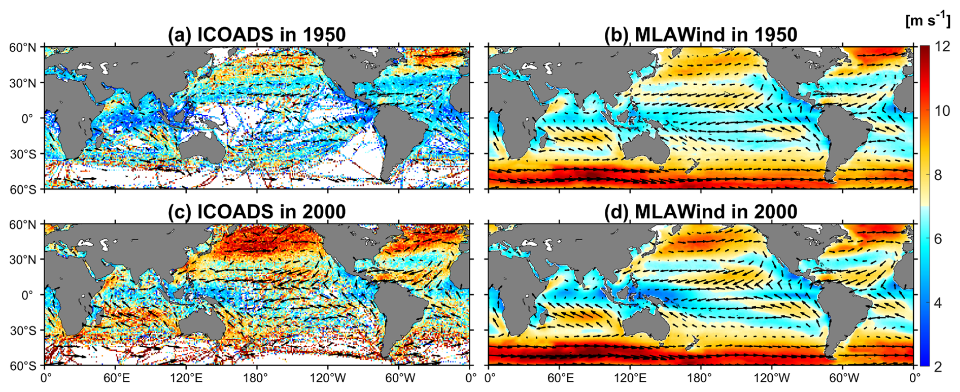
Figure 3 Reconstruction results presentation. 10-m wind velocity (vector, m s⁻¹) and sea surface wind speed (shading, m s⁻¹) of the original ICOADS and MLAWind dataset are compared in 1950 and 2000, respectively. These 2 years are chosen as examples to represent periods with sparse and abundant original data coverage, respectively.

The second step is establishing a pre-trained model integrating the SHAP algorithm to achieve synergistic optimization of model efficiency and interpretability. Specifically, the feature set comprising multiple wind-related variables and their spatiotemporal information is input into a pre-trained model. The SHAP algorithm quantifies the contribution of each feature to the model's output, thereby establishing a feature importance ranking (Lundberg and Lee, 2017). The top-K (e.g., 5–10) highest-contributing features are retained, while redundant variables with relative contribution below 10 % are eliminated to reduce model complexity and enhance physical interpretability. Based on the SHAP analysis, the ICOADS 10-m zonal wind, meridional wind, SST, WS, longitude, latitude, and month are identified as the seven key feature variables for sea surface wind reconstruction. They are utilized to establish a lightweight model, while other variables with little contribution (i.e. T_a, SLP and year) are excluded.

Thirdly, the lightweight model is trained from 1993–2022, facilitating point-to-point learning between ICOADS variables and CCMP sea surface winds. Parameter tuning, K-fold Cross Validation, and generalization capability validation are three key components for lightweight models: (1) a grid search approach is employed to identify the optimal model parameters. Consequently, the number of regression trees, the minimum number of samples required to split and samples required to be at a leaf node is set to 200, 3, 3, respectively; (2) leave-one-out Cross Validation (LOOCV), a specialized form of K-fold Cross Validation is implemented during the model establishment process (Mao et al., 2014). The 30-year samples from 1993–2022 are segmented into 30 submodels, with each submodel consisting of a 29-year training set and a 1-year validation set. LOOCV exhibits minimal discrepancies among these model, indicating the lightweight model's robust performance; (3) an independent verification is conducted in 2023 to evaluate model's generalization capability. The results will be presented in Sect. 3.

The final step is the model inference process that generates the restructured dataset. The process operates without label variable. Following the training process conducted from 1993–2022, the machine learning model derives a nonlinear relationship between ICOADS variables and CCMP sea surface wind. The established relationship enables the reconstruction of historical sea surface winds during the non-satellite periods by utilizing ICOADS data from 1950–1992. The resultant monthly MLAWind dataset spanning 1950 to 2023, covering near-global oceans between 60° S and 60° N at a horizontal resolution of 1° × 1°.

Figure 3 exhibits the reconstruction efficacy in 1950 and 2000. The two years are chosen as examples to represent periods with sparse and abundant original data coverage, respectively (Fig. 1). The original ICOADS from 1950 exhibits significant spatial data gaps, particularly in the tropical Pacific and Southern Ocean. MLAWind shows continuous spatial coverage. Despite limited observations in the Southern Ocean, it demonstrates robust reconstruction of the prevailing westerly wind belt (Garreaud et al., 2013). In 2000, ICOADS exhibits a higher spatial density, while still containing considerable noise. MLAWind demonstrates smoother sea surface wind characteristics. The CCMP satellite observation is used to evaluate the biases of ICOADS and MLAWind in 2000. ICOADS exhibits significant systematic biases, primarily attributed to uncertainties in ship height measurements and instrumental calibration protocols (Berry and Kent, 2011; Tokinaga and Xie, 2011). MLAWind effectively mitigates these biases and demonstrates high consistency with the CCMP, confirming the validity of the reconstruction.

2.4 Evaluation metrics

Five metrics are employed in the evaluation process, including mean error (Bias), root mean square error (RMSE), Pearson correlation coefficient (CORR), skewness and the coefficient of determination (R-squared). Bias, RMSE and CORR quantify discrepancies between observations and products. Skewness characterizes the asymmetry of a variable's probability distribution. Positive values denote right-skewed distributions with longer tails toward large values and a left-shifted peak. R-square serves as a key metric for assessing model performance. Its values span from 0 to 1, with those closer to 1 indicating better model performance. These metrics can be described as follows:

$$\begin{array}{}\text{(1)}& {\displaystyle }& {\displaystyle }\text{Bias}={\displaystyle \frac{\mathrm{1}}{n}}{\sum }_{i=\mathrm{1}}^n\left(y_i-{\widehat{y}}_i\right)\text{(2)}& {\displaystyle }& {\displaystyle }\text{RMSE}=\sqrt{{\displaystyle \frac{\mathrm{1}}{n}}{\sum }_{i=\mathrm{1}}^n{\left(y_i-{\widehat{y}}_i\right)}^{\mathrm{2}}}\text{(3)}& {\displaystyle }& {\displaystyle }\text{CORR}={\displaystyle \frac{{\sum }_{i=\mathrm{1}}^n\left(y_i-\stackrel{\mathrm{‾}}{y}\right)\left({\widehat{y}}_i-\stackrel{\mathrm{‾}}{\widehat{y}}\right)}{\sqrt{{\sum }_{i=\mathrm{1}}^n{\left(y_i-{\widehat{y}}_i\right)}^{\mathrm{2}}}\sqrt{{\sum }_{i=\mathrm{1}}^n{\left({\widehat{y}}_i-\stackrel{\mathrm{‾}}{\widehat{y}}\right)}^{\mathrm{2}}}}}\text{(4)}& {\displaystyle }& {\displaystyle }\text{Skewness}={\displaystyle \frac{\sqrt{n(n-\mathrm{1})}}{n-\mathrm{2}}}{\displaystyle \frac{\frac{\mathrm{1}}{n}{\sum }_{i=\mathrm{1}}^n{\left(y_i-\stackrel{\mathrm{‾}}{y}\right)}^{\mathrm{3}}}{{\left(\sqrt{\frac{\mathrm{1}}{n}{\sum }_{i=\mathrm{1}}^n{\left(y_i-\stackrel{\mathrm{‾}}{y}\right)}^{\mathrm{2}}}\right)}^{\mathrm{3}}}}\text{(5)}& {\displaystyle }& {\displaystyle }{R}^{\mathrm{2}}=\mathrm{1}-{\displaystyle \frac{{\sum }_{i=\mathrm{1}}^n{\left(y_i-{\widehat{y}}_i\right)}^{\mathrm{2}}}{{\sum }_{i=\mathrm{1}}^n{\left(y_i-\stackrel{\mathrm{‾}}{\widehat{y}}\right)}^{\mathrm{2}}}}\end{array}$$

where n represents the number of samples, y_i represents the values obtained from different products, ${\widehat{y}}_i$ represents observational values. $\stackrel{\mathrm{‾}}{y}$ and $\stackrel{\mathrm{‾}}{\widehat{y}}$ represent the mean values of y_i and ${\widehat{y}}_i$, respectively.

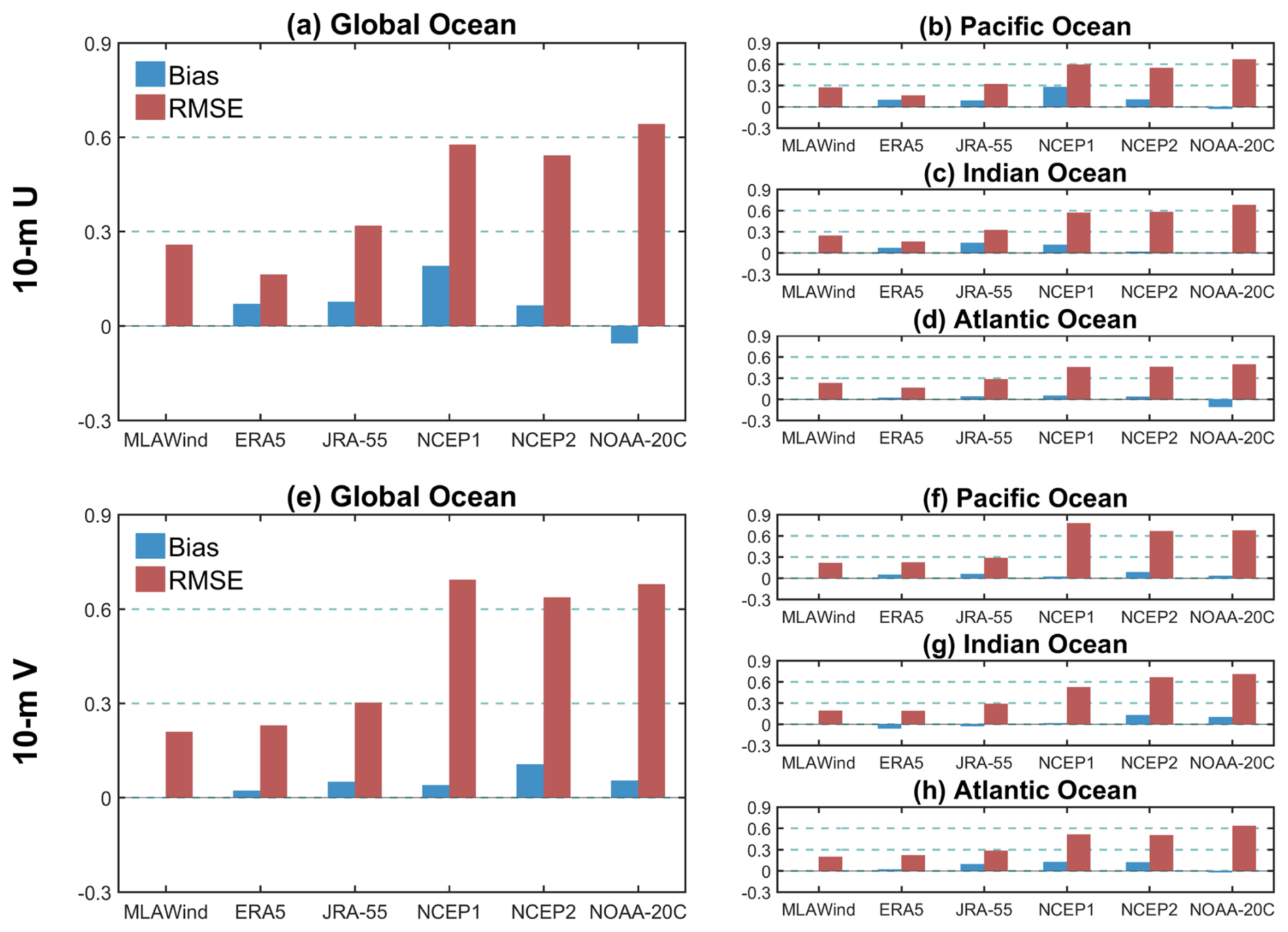
Figure 4 Evaluation based on satellite sea surface wind. (a–d) Bias and RMSE values (m s⁻¹) of multiple datasets evaluated with CCMP 10-m zonal wind over different oceans within 60° S–60° N from 1993–2022. (e–h) Same as (a–d) but for 10-m meridional wind.

3 Evaluation of the MLAWind dataset

Based on satellite data, we systematically evaluate the performance of the MLAWind dataset on the training set (1993–2022) and testing set (2023), respectively (Figs. 4–6). During the training period, the MLAWind dataset shows the smallest mean biases for both 10-m zonal and meridional winds (Fig. 4a and e). It achieves the lowest RMSE (0.21 m s⁻¹) for meridional wind, while its RMSE (0.26 m s⁻¹) ranks second only to the ERA5 dataset (0.16 m s⁻¹) for zonal wind. The mean bias and RMSE are quantified across the Pacific, Indian, and Atlantic Oceans. Their performance is comparable to those of near-global coverage for both 10-m zonal (Fig. 4b–d) and meridional wind (Fig. 4f–h). A global evaluation of WD is performed to further confirm the reliability of the MLAWind dataset. The MLAWind dataset demonstrates the lowest mean bias and the second-lowest RMSE across all evaluated products. Despite the absence of direct reconstruction of WD, the MLAWind dataset derives WD with high accuracy.

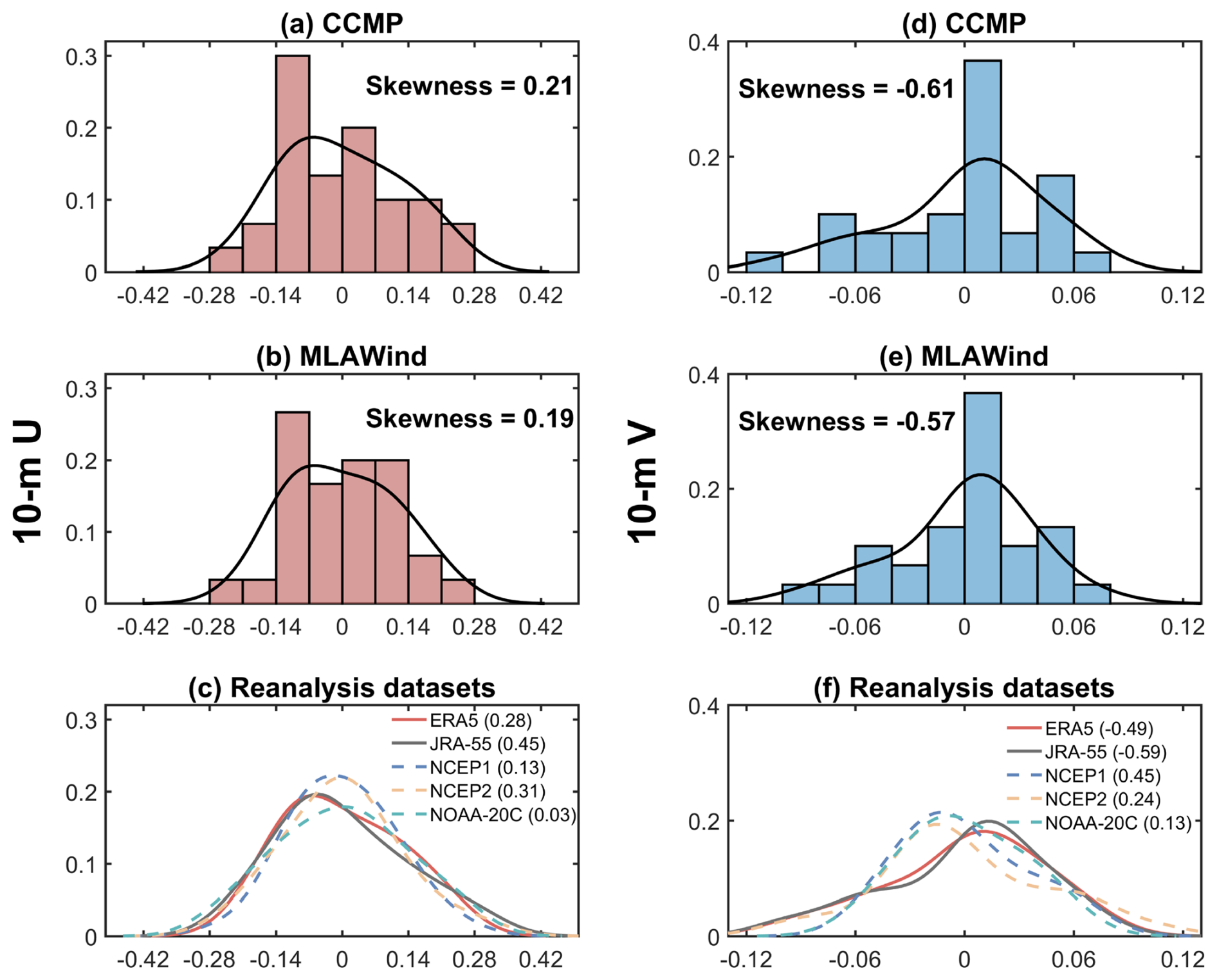
Figure 5 Comparison of probability density functions (PDF) among different datasets. (a–c) PDF and skewness coefficients of 10-m zonal wind in different datasets from 1993–2022. The horizontal axis denotes 10-m zonal wind anomalies. The vertical axis denotes probability densities. The values in parentheses in (c) denote skewness coefficients of reanalysis datasets. (d–f) Same as (a-c) but for 10-m meridional wind.

The probability density function (PDF) characteristics of different sea surface wind datasets are compared from 1993–2022. The 10-m zonal wind in CCMP, MLAWind, and reanalysis datasets collectively exhibit positive skewness distributions with longer tails toward larger values and left-shifted peaks (Fig. 5a–c). MLAWind demonstrates the closest skewness value (0.19) to CCMP satellite data (0.21) among all datasets. The 10-m meridional wind in MLAWind and CCMP are consistent in their negative skewness distributions, whereas substantial divergences emerge across reanalysis datasets (Fig. 5d–f). In contrast to the CCMP dataset, the 10-m meridional wind in NCEP1, NCEP2, and NOAA-20C exhibit positive skewness in their distributions (Fig. 5f), which may be attributed to their large RMSE with satellite data (Fig. 4).

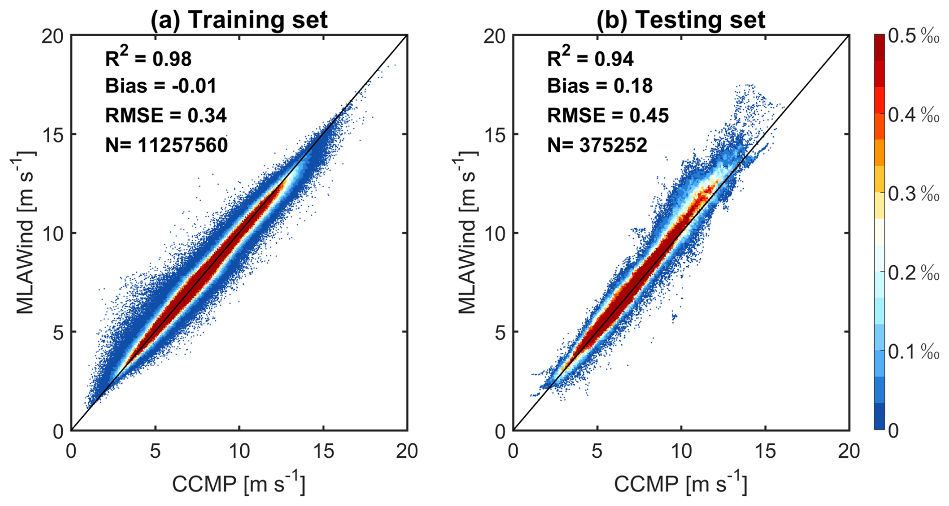
Figure 6 Validation of MLAWind's generalization capability. Density scatter plots compare the MLAWind and CCMP datasets during (a) training phase (1993–2022) and (b) testing phase (2023), respectively. The shading represents data density within each bin. R², mean bias, RMSE and sample size (N) are used as quantitative metrics for evaluating MLAWind's performance.

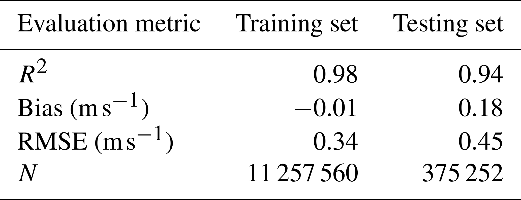
During the testing phase, the MLAWind dataset maintains strong agreement with satellite observations in 2023 (Fig. 6b). Most values fall near the 1:1 reference line, with relatively larger errors under high wind conditions (≥ 15 m s⁻¹). The mean bias and RMSE between the MLAWind and CCMP datasets are 0.18 and 0.45 m s⁻¹, respectively. Notably, the MLAWind dataset achieves R-squared values exceeding 0.90 for both the training and testing sets (Table 2). The high consistency exhibits its robust generalization capabilities without signs of overfitting.

Table 2 Comparison of MLAWind's performance on the training set (1993–2022) and testing set (2023). ‌The CCMP satellite data is used as the evaluation benchmark.

Figure 7 Evaluation of multiple datasets based on the GTMBA observations from 1993–2023.

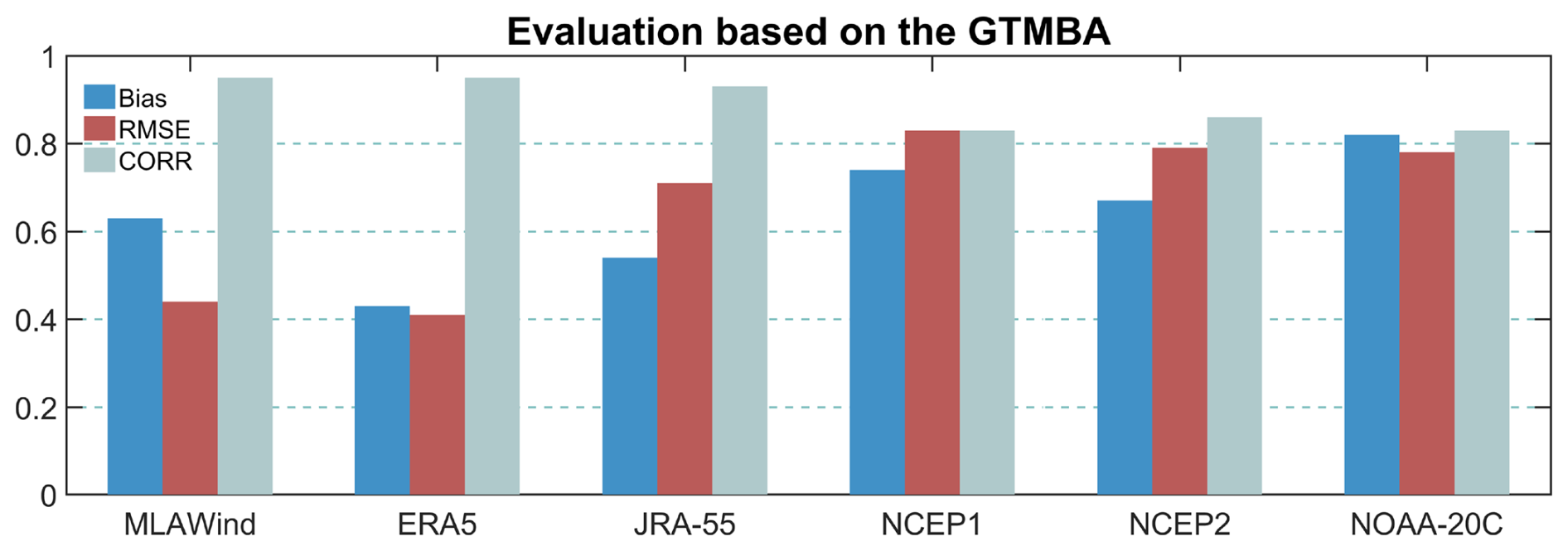
In addition to satellite data, the performance of multiple datasets from 1993 to 2023 is compared based on the GTMBA in-situ observations (Fig. 7). MLAWind and ERA5 demonstrate high consistency with the GTMBA, exhibiting smaller errors than other datasets. These two datasets equally achieve low RMSE (∼ 0.40 m s⁻¹) and high CORR (0.95), although MLAWind demonstrates a slightly larger bias than ERA5. Note that ERA5 assimilates the GTMBA and thus its evaluation results are not independent. MLAWind achieves reconstruction accuracy comparable to ERA5, without relying on in-situ buoy observations.

4 Performance of MLAWind from climatology to long-term trend

The reliability of the MLAWind dataset is validated through satellite and in-situ observations in both training and non-training periods (Figs. 4–7). In this section, the performance of the MLAWind dataset since 1950 are assessed across different time scales, including climatology, seasonality, inter-annual variations, and long-term trends. Its similarities and differences with reanalysis datasets are evaluated, particularly during the period without satellite data.

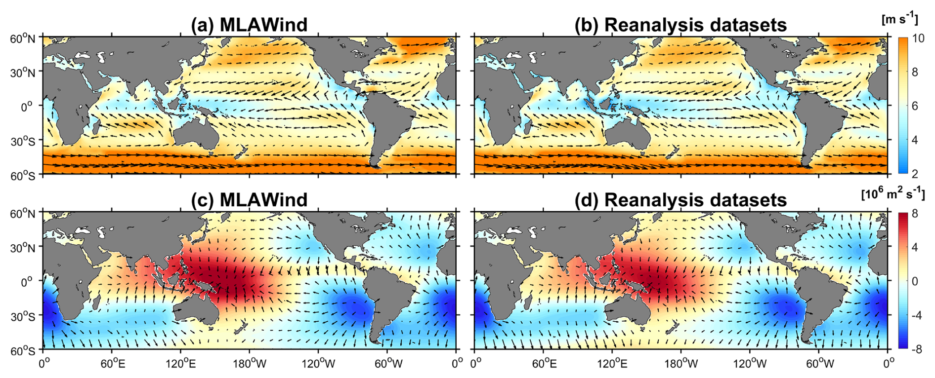
Figure 8 (a, b) Climatology of 10-m wind velocity (vector, m s⁻¹) and sea surface wind speed (shading, m s⁻¹) in the MLAWind dataset and the reanalysis datasets from 1981 to 2010. (c, d) Same as (a, b) but for divergent wind (vector, m s⁻¹) and velocity potential (shading, m² s⁻¹). The 30-year period is selected because all datasets are available during this period (Table 1). The climatological distribution of the MLAWind dataset over the 73-year period from 1950 to 2022 are examined and show no significant differences.

4.1 Climatology and annual cycle

The climatological spatial pattern of the MLAWind dataset aligns closely with those of multiple reanalysis products, demonstrating robust consistency in capturing the tropical trade wind belt and the mid-latitude westerly belt (Fig. 8a and b). Moreover, it can reproduce the key dynamical features of atmospheric circulation. The divergent wind and velocity potential of the MLAWind dataset exhibit a well-defined convergence–divergence dipole structure of the Walker circulation: intense convergence is concentrated over the Indo–Pacific Warm Pool, while robust divergence centers are distinctly localized in the southeastern Pacific Ocean (Fig. 8c).

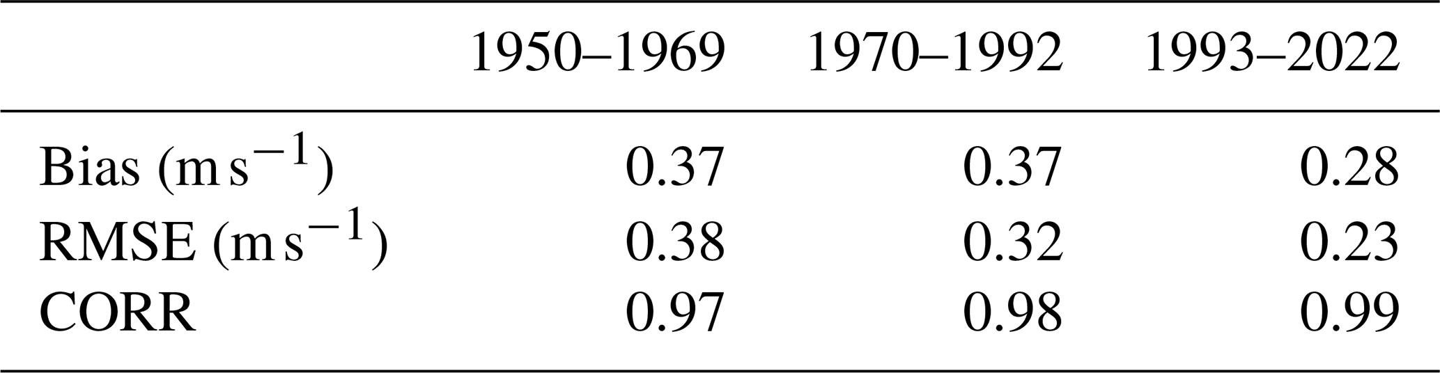
The climatological distributions between the MLAWind dataset and the reanalysis datasets are further compared across three distinct periods (i.e. 1950–1969, 1970–1992, and 1993–2022). Similar to Fig. 8, the spatial distributions of MLAWind are highly consistent with those of the reanalysis datasets, even during the pre-satellite periods (1950–1969 and 1970–1992). Both datasets capture prominent westerlies over the Kuroshio, Gulf Stream, and mid-latitude Southern Hemisphere. They reproduce the strong easterlies over the equatorial Pacific and Atlantic, together with the weak annual-mean winds over the equatorial Indian Ocean that arise from monsoon-driven seasonal reversals (Schott et al., 2009). The quantitative evaluation indicates that global-mean climatological sea surface wind speed of the MLAWind dataset exhibits low bias and RMSE relative to the reanalysis datasets, accompanied by a high correlation above 0.97 over the three examined periods (Table 3).

Table 3 Comparison of global-mean climatological sea surface wind speed between the MLAWind dataset and the reanalysis datasets across different periods.

The standard deviations of the 10-m zonal and meridional wind anomalies derived from the MLAWind dataset and the reanalysis datasets are assessed across different periods. The MLAWind dataset exhibits strong spatial consistency with the reanalysis datasets, despite differences in magnitude. Both datasets consistently indicate that high-variability regions are confined to the westerly wind belt and the Indo–Pacific Warm Pool region. These results demonstrate that the MLAWind dataset effectively captures the variability of sea surface winds, even during periods with sparse satellite data and in regions with limited observations.

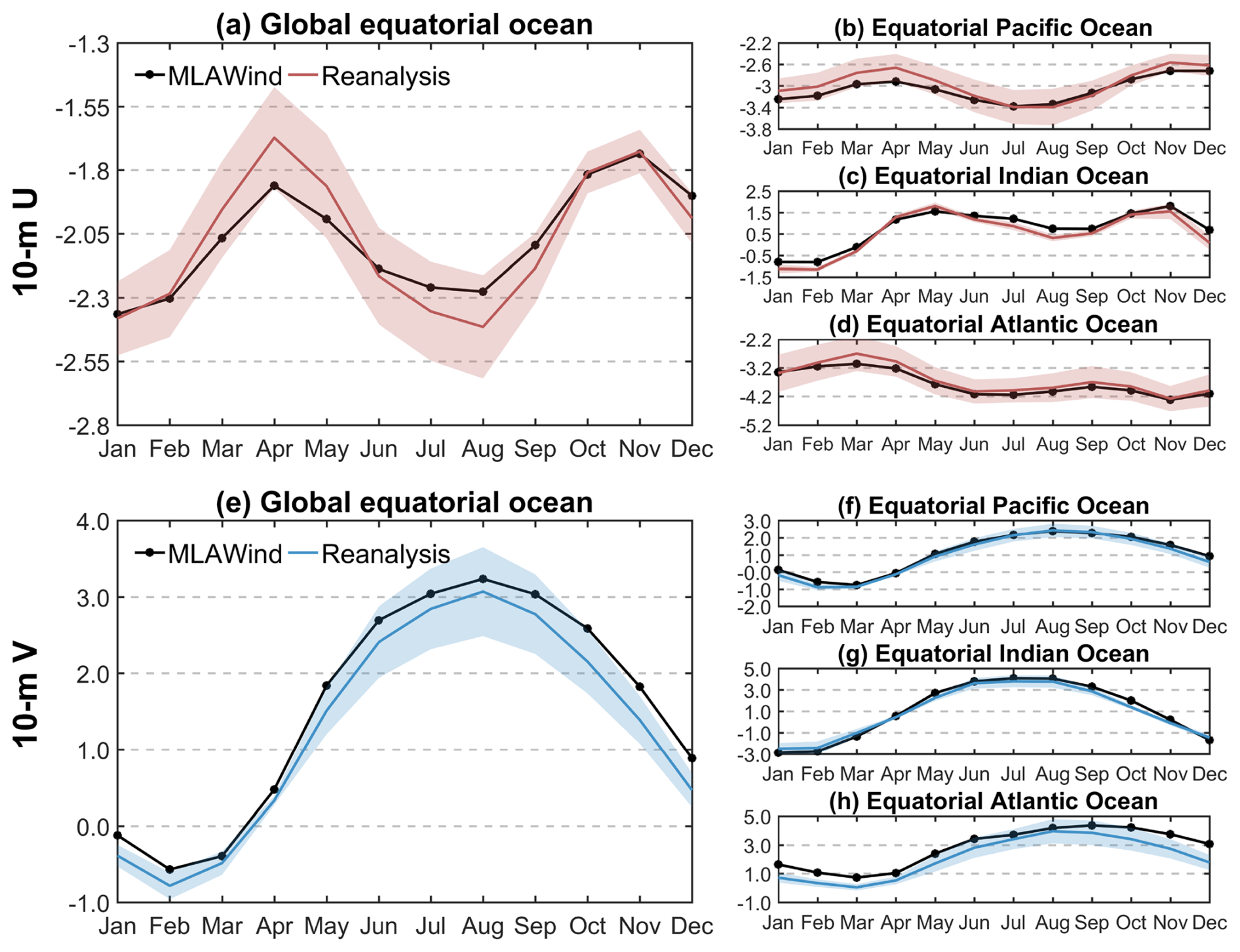
Figure 9 Annual cycle of sea surface wind (m s⁻¹) over equatorial oceans (5° S–5° N) from 1981 to 2010: (a–d) 10-m zonal wind and (e–h) 10-m meridional wind. The red shadings in (a–d) and the blue shading in (e–h) denote one standard deviations of 10-m zonal and meridional winds from multiple reanalysis datasets, respectively. The 30-year period (1981–2010) is selected because all datasets are available during this period (Table 1). The annual cycle of the MLAWind dataset over the 73-year period from 1950 to 2022 are examined and show no significant differences.

The annual cycle of mean sea surface winds is evaluated in equatorial regions within 5° S–5° N (Fig. 9). The 10-m zonal winds in the MLAWind dataset and reanalysis datasets show similar seasonal variations over the global equatorial ocean, with their easterlies persisted within a range of 1.55–2.55 m s⁻¹ throughout the year. A discrepancy in intensity exists between the two datasets. The 10-m zonal winds in the MLAWind dataset exhibit stronger easterlies during March–May and weaker easterlies during July–September compared to reanalysis datasets (Fig. 9a). The annual cycle characteristics of the MLAWind dataset show a general agreement with those of reanalysis datasets over the three equatorial oceans, albeit with some differences in magnitude (Fig. 9b–d). The 10-m meridional wind in both the MLAWind dataset and reanalysis datasets display a distinct unimodal structure, featuring a southerly wind peak in February and a northerly wind peak in August (Fig. 9e). The MLAWind dataset accurately captures the annual cycle of 10-m meridional winds across different equatorial oceans, consistent with reanalysis datasets (Fig. 9f–h).

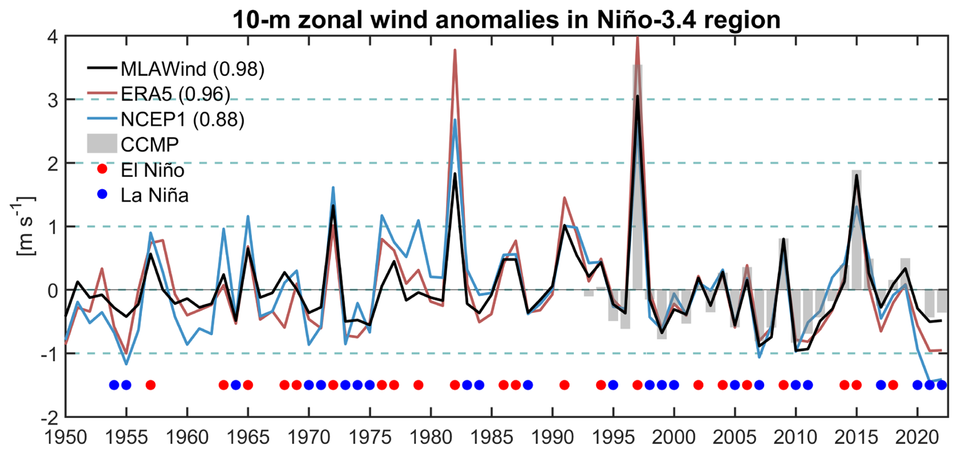
Figure 10 Inter-annual variations of the November–December mean 10-m zonal wind anomalies (m s⁻¹) over the Niño-3.4 region (5° S–5° N, 170–120° W). Long-term linear trends from 1950–2022 are removed. The grey bars denote 10-m zonal wind anomalies of CCMP from 1993–2022. The values in parentheses denote correlation coefficients with the CCMP data. The red and blue circles denote El Niño and La Niña events, respectively. El Niño and La Niña events are defined when the November–December mean Niño-3.4 index ≥ +0.5 and ≤ −0.5 °C, respectively.

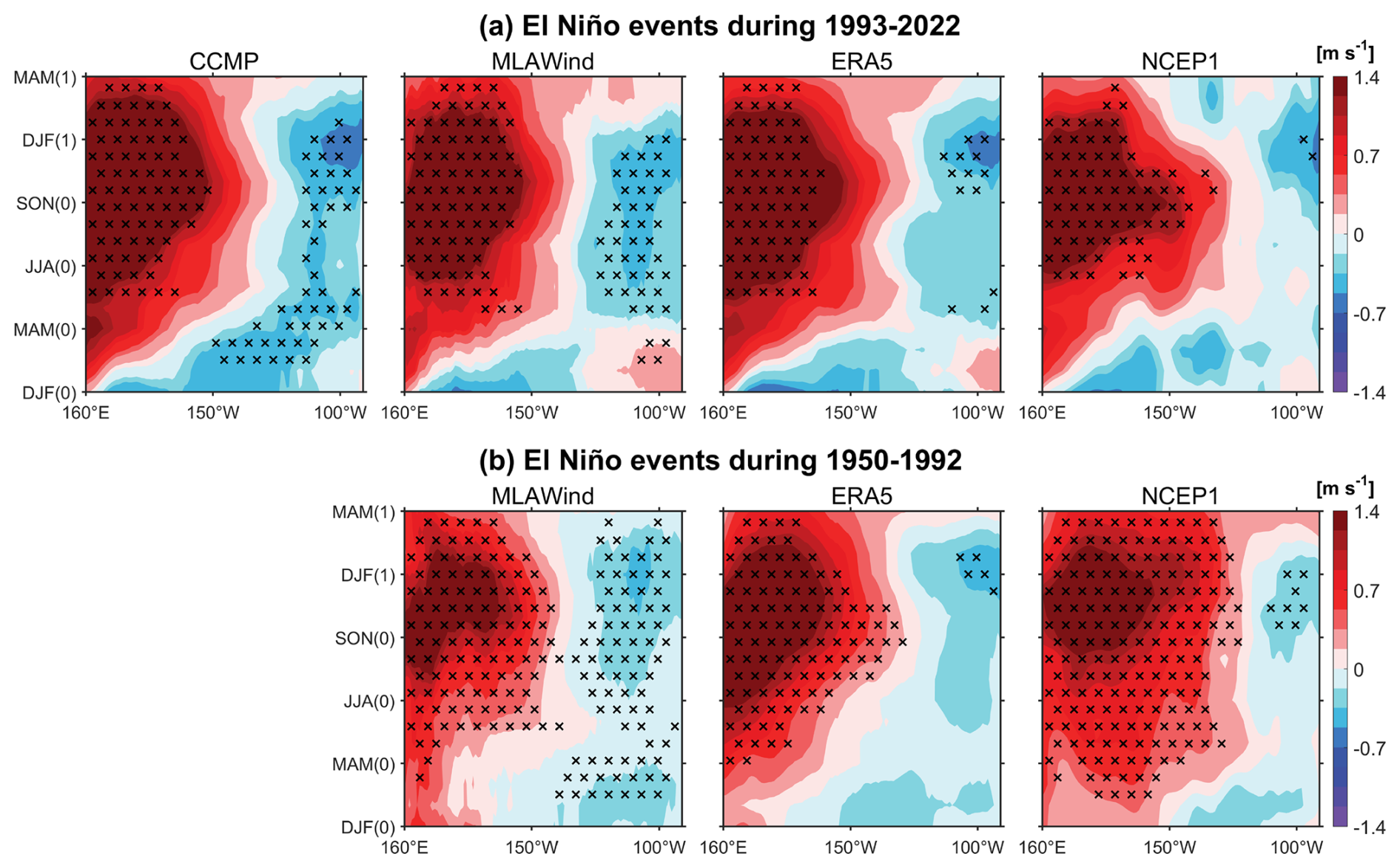
Figure 11 Composites of meridional mean (5° S–5° N) of 10-m zonal wind anomalies. (a) El Niño events during 1993–2022. (b) Same as (a) but for the period lacking satellite data (1950–1992). DJF(0)-SON(0) denote the periods in the developing year while DJF(1)-MAM(1) denote the periods in the decaying year. The black crosses denote the composites exceeding the 99 % significance level based on Student's t-test.

4.2 Inter-annual variabilities

ENSO is the dominant inter-annual climate variability in the tropics, exerting significant influences on both regional and global climate systems (e.g. Bjerknes, 1969; Trenberth et al., 1998; McPhaden et al., 2006). Sea surface wind anomalies are greatly associated with the ENSO cycle (Bjerknes, 1969; McPhaden et al., 2006; Kug et al., 2009). Time series of 10-m zonal wind anomalies from multiple datasets are compared over the Niño-3.4 region (Fig. 10). During the satellite observation period (1993–2022), MLAWind, ERA5, and NCEP1 show strong agreement with CCMP, among which MLAWind exhibits the highest correlation coefficient (CORR = 0.98). During the historical period lacking satellite data (1950–1992), MLAWind maintains comparable inter-annual variations to those of both ERA5 and NCEP1, while demonstrating a higher correlation coefficient with the Niño-3.4 index (CORR = −0.86). The 10-m zonal wind anomalies derived from MLAWind show a robust association with ENSO dynamics, exhibiting strong westerly wind anomalies during El Niño events and persistent easterly anomalies during La Niña events, which aligns closely with the canonical Bjerknes feedback mechanism (Bjerknes, 1969; McPhaden et al., 2006; Kug et al., 2009). Moreover, the inter-annual variabilities of MLAWind across other tropical ocean basins have been validated, equally exhibiting high consistency with reanalysis datasets and SST variabilities (Guo et al., 2025a).

A composite analysis of El Niño events is conducted for the satellite (Fig. 11a) and non-satellite periods (Fig. 11b). The selected El Niño events are marked by red circles in Fig. 10, with a total of 13 events during 1950–1992 and 8 events during 1993–2022. During the satellite period (1993–2022), MLAWind reveal the development of westerly wind anomalies over the equatorial central-western Pacific Ocean (5° S–5° N, 160° E–150° W), peaking around DJF(1). Weak easterly wind anomalies are observed over the equatorial eastern Pacific Ocean (5° S–5° N, 150–90° W). The pattern is consistent with those of CCMP, with the spatial correlation coefficient exceeding 0.95. ERA5 and NCEP1 exhibit pronounced westerly anomalies in the region west of 150° W, but the easterly anomalies in the equatorial eastern Pacific Ocean are weaker than those of CCMP and MLAWind (Fig. 11a).

During the historical period of 1950–1992, both MLAWind and reanalysis datasets show comparable sea surface wind patterns to those observed during the satellite period. They collectively demonstrate significant westerly wind anomalies that are strongly linked to the development of El Niño events (Fig. 11b). It is noted that there are several discrepancies in the three datasets. MLAWind shows relatively stronger easterly anomalies in the eastern equatorial Pacific Ocean. NCEP1 exhibits more pronounced westerly anomalies during the DJF(0)-MAM(0) period, which extends further eastward compared to those of MLAWind and ERA5 (Fig. 11b). Although the absence of robust benchmarks hinders the assessment of their relative accuracy, the consistency with satellite data and the Niño-3.4 index (Fig. 10) suggests that MLAWind may provide more reliable sea surface wind variations.

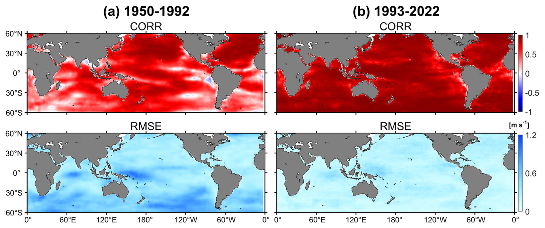
Figure 12 (a) Correlation coefficient (CORR) and Root Mean Square Error (RMSE) between MLAWind and ERA5 for 10-m zonal winds during 1950–1992. (b) Same as (a) but for 1993–2022.

In addition to the tropical Pacific Ocean, the inter-annual variability of the MLAWind dataset is systematically assessed on a global scale. Figure 12 presents the CORR and RMSE between MLAWind and ERA5. During 1993–2023, the 10-m zonal winds from MLAWind exhibit the strongest positive correlations with those from ERA5, which can be attributed to the incorporation of CCMP satellite data in the generation of both datasets (Hersbach et al., 2019). During 1950–1992, MLAWind maintains significant positive correlations with ERA5 over most of the globe. It indicates that MLAWind can effectively reproduce the inter-annual variability characteristics of reanalysis datasets, even in the absence of satellite data (Fig. 12).

The 10-m zonal wind of MLAWind exhibits minimal RMSE values during the satellite period. During 1950–1992, its RMSE remains modest over most of the global ocean, with relatively large values concentrated in the Southern Ocean and the eastern tropical Indian Ocean (Fig. 12). The pronounced discrepancies over the Southern Ocean can be attributed to the sparse observational coverage within the 30–60° S band, which introduces substantial uncertainties across all products. In addition, previous study has revealed considerable uncertainties among different datasets in the tropical Indian Ocean, where MLAWind are found to be more reliable than the existing reanalysis datasets (Guo et al., 2025a).

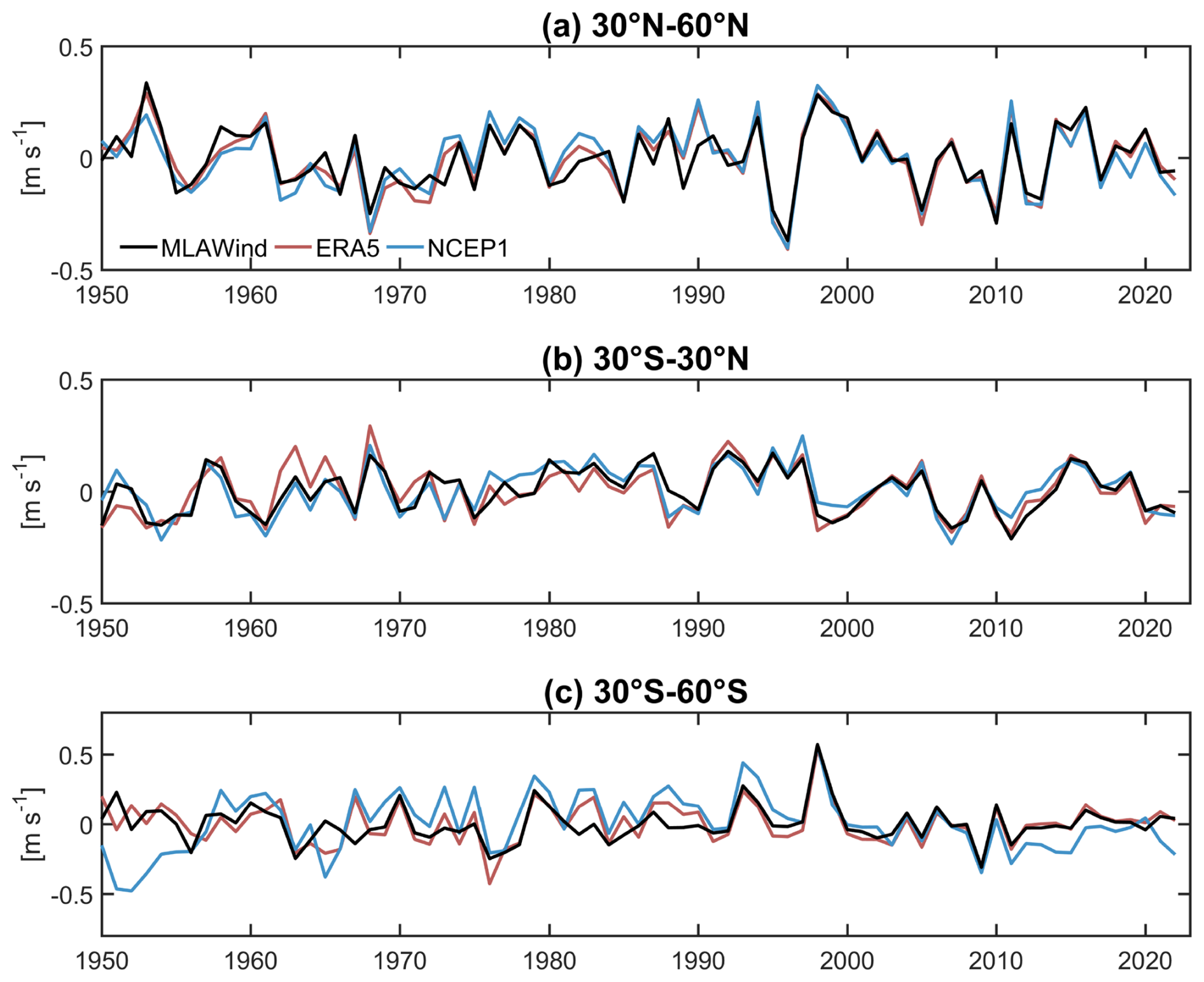
Figure 13 Inter-annual variations of the 10-m zonal wind anomalies (m s⁻¹) across different latitude bands. Long-term linear trends from 1950–2022 are removed.

To further compare the performance of the MLAWind dataset and the reanalysis datasets in different regions, their inter-annual variations are assessed across three broad latitude bands: 30–60° S, 30° S–30° N, and 30–60° N (Fig. 13). The 10-m zonal wind anomalies from MLAWind exhibit strong temporal consistency with those from reanalysis datasets across different regions, even during periods without satellite observations. Despite the relatively large RMSE between MLAWind and ERA5 over the westerly wind belt in the Southern Hemisphere (Fig. 12), MLAWind is effective in capturing the inter-annual variability of the 10-m zonal wind anomalies within the 30–60° S region (Fig. 13c). The result demonstrates that MLAWind maintain robust applicability during non-satellite periods and over the Southern Ocean. It can serve as a reliable data source for global wind field change studies.

Table 4 Long-term trends of coral $\mathrm{Mn}/\mathrm{Ca}$ and 10-m zonal wind surrounding Tarawa Atoll (4° S–6° N, 166–176° E) from 1950–1982. Positive values of coral $\mathrm{Mn}/\mathrm{Ca}$ indicate an intensification of westerly winds. The temporal correlation coefficients between $\mathrm{Mn}/\mathrm{Ca}$ and multiple datasets are assessed. All datasets are smoothed using a 11-year running mean filter to remove the impact of high-frequency signals.

4.3 Long-term trends

The long-term trend can filter the interference from short-term fluctuations, and thus reveal the linear change over a long time span (usually decades or longer periods). The long-term trends of the MLAWind dataset are evaluated in both the satellite (after 1993) and non-satellite (before 1993) periods to analyze its reliability across the two periods. The analysis during 1993–2022 reveals that the MLAWind dataset attains the most robust spatial concordance with observations among all evaluated datasets (CORR = 0.95). This strong agreement is due to its low bias and RMSE with satellite data (Fig. 4).

The long-term trends among different products exhibit significant divergence during historical periods without satellite data (Guo et al., 2025a). Coral records are used to assess the performance of sea surface wind during these periods. The skeletal $\mathrm{Mn}/\mathrm{Ca}$ ratio in corals from atolls with west-facing lagoons serves as an effective proxy for identifying westerly wind anomalies (Shen et al., 1992), thereby reflecting the strength and variability of zonal winds at both inter-annual and multi-decadal time scales (Thompson et al., 2015). The employed coral $\mathrm{Mn}/\mathrm{Ca}$ records are collected from three distinct sites in the tropical Pacific Ocean, including Tarawa Atoll (1.33° N, 172.97° E), Butaritari Atoll (3.07° N, 172.75° E) and Kiritimati Island (1.93° N, 157.49° W).

The coral $\mathrm{Mn}/\mathrm{Ca}$ records from Tarawa Atoll (4° S–6° N, 166–176° E) provide a valuable proxy for the period of 1950–1982, when satellite observations are unavailable. The pronounced increasing trend in $\mathrm{Mn}/\mathrm{Ca}$ ratios from 1950 to 1982 suggests an intensification of the westerlies, yet it does not afford a quantitative estimate of the magnitude of sea surface wind variability. Significant uncertainties remain in the long-term trends across multiple datasets (Table 4), primarily attributed to discrepancies in their data assimilation models and technical approaches. Consistent with $\mathrm{Mn}/\mathrm{Ca}$ records, the MLAWind and ERA5 datasets reveal a significant strengthening of westerly winds (p<0.05), with a more pronounced trend observed in the MLAWind dataset. The trends derived from the NCEP1 and NOAA-20C datasets are weaker and statistically insignificant, demonstrating their relatively lower reliability for the period lacking satellite data. Moreover, the positive temporal correlation between MLAWind and $\mathrm{Mn}/\mathrm{Ca}$ surrounding Tarawa Atoll is much stronger than those observed in ERA5, NCEP1, and NOAA-20C, indicating that MLAWind provides a more reliable and physically consistent reconstruction of long-term sea surface wind variability during non-satellite periods (Table 4). Two supplementary $\mathrm{Mn}/\mathrm{Ca}$ records from Butaritari Atoll (1989–2010) and Kiritimati Island (1994–2011) are also examined. The MLAWind dataset likewise exhibits strong agreement with the long-term trends of these records.

A comprehensive analysis of sea surface wind trends in the tropical Indian Ocean (TIO) reveals significant discrepancies among multiple datasets (Guo et al., 2025a). Different from reanalysis results, the MLAWind dataset exhibits a significant weakening of sea surface wind speed over the TIO during 1950–2019. The trend is corroborated by the asymmetrical west-east variations in both thermocline depth and sea surface height since 1950 (Guo et al., 2025a), demonstrating the reliability of the MLAWind dataset in capturing sea surface wind variations over long time periods.

5 Data availability

The MLAWind dataset reconstructed in this study is available at https://doi.org/10.5281/zenodo.17354864 (Guo et al., 2025b) and https://doi.org/10.12157/IOCAS.20250707.001 (Guo et al., 2025c). Here, we provide a monthly gridded sea surface wind product at 1° × 1° horizontal resolution from 1950 to 2023, covering the near-global ocean between 60° S and 60° N.

6 Conclusions

This study employs a random forest algorithm integrated with the SHAP interpretable module to generate a monthly sea surface wind dataset (MLAWind). The MLAWind dataset effectively combines the respective strengths of in-situ and remote sensing observations, covering the near-global ocean between 60° S and 60° N from 1950 to 2023, with a spatial resolution of 1° × 1°. The evaluations based on satellite data reveal that MLAWind exhibits better agreement with observations during the training period (1993–2022) compared to most reanalysis datasets. It shows strong generalization capability, maintaining robust performance during the testing period (2023). The performance of MLAWind since 1950 is evaluated across different time scales, including climatology, annual cycle, inter-annual variation, and long-term trends. The assessments based on reanalysis datasets and coral records indicate that MLAWind demonstrates better skill in capturing long-term variations of sea surface winds compared to other datasets. MLAWind is expected to become an important resource for global climate change research.

The MLAWind dataset will continue to be optimized and updated in future work. The current version of the MLAWind dataset is limited within 60° S–60° N, owing to the insufficient data coverage of the ICOADS and CCMP datasets in high-latitude regions. More reliable high-latitude datasets will be integrated into the machine learning model in the future, enabling the development of a global sea surface wind dataset. In addition, the MLAWind dataset, currently available at a horizontal resolution of 1° × 1°, demonstrates robust capability in capturing large-scale circulation signals. Further enhancement of its spatial resolution to 0.25° × 0.25° will significantly advance mesoscale marine and climate research. Several potential approaches can be used to construct a higher-resolution version of the MLAWind dataset, including the integration of higher-resolution input variables (Tian et al., 2022), the application of machine learning-based interpolation (He et al., 2022) and super-resolution techniques (Wang et al., 2021; Doury et al., 2023). An assessment of diverse approaches will be conducted in future work to ensure the upcoming high-resolution MLAWind dataset retains the existing version's accuracy while capturing mesoscale atmospheric processes.