RRBF-KMA: high-resolution radar–gauge merged precipitation dataset for South Korea (2016–2024)

This study presents a long-term, high-resolution precipitation dataset over South Korea generated by merging nationwide composite radar reflectivity with dense rain gauge observations from the Korea Meteorological Administration (KMA). The dataset provides precipitation at 10 min temporal resolution and 0.5 km spatial resolution on a regular grid of 2305 pixels × 2881 pixels, covering the period from 2016 to 2024.

Rain gauge observations, originally recorded at 1 min intervals, are quality-controlled and aggregated to 10 min accumulations prior to merging. Radar inputs are obtained from the nationwide composite reflectivity product provided by KMA. To ensure temporal consistency in the merged precipitation fields, a radar–gauge bias correction scheme is applied in which scaling factors are updated at 10 min intervals during precipitation events and constrained relative to preceding time steps. This approach reduces spurious temporal variability while maintaining sensitivity to evolving precipitation systems.

Residual differences between bias-corrected radar estimates and gauge observations are interpolated using a Residual Radial Basis Function (RRBF) method. The method models spatially structured residuals to preserve fine-scale radar-derived variability while incorporating gauge-based corrections. The entire merging procedure is computationally efficient, requiring approximately one minute per 10 min analysis, which supports near-real-time implementation.

The resulting product provides temporally continuous and spatially consistent precipitation fields suitable for hydrological applications, extreme rainfall analysis, and urban flood forecasting. The dataset, together with detailed documentation of the generation and validation procedures, is publicly available for research and operational use. The dataset is publicly available at https://doi.org/10.5281/zenodo.19491708 (Ryu et al., 2026a) and https://doi.org/10.5281/zenodo.19562910 (Ryu et al., 2026b).

1 Introduction

High-resolution precipitation datasets are essential for meteorological and hydrological applications, including flood forecasting, hydrological modeling, and urban water management (Kidd and Huffman, 2011; Ochoa-Rodriguez et al., 2019). In particular, sub-hourly and kilometer-scale rainfall estimates are required to resolve localized heavy rainfall events that can trigger flash floods and produce severe impacts in highly urbanized regions.

Several long-term radar-based precipitation datasets have been developed at national and continental scales, including RADKLIM over Germany (Winterrath et al., 2018), the UK Met Office NIMROD radar composite (Met Office, 2003), the European OPERA composites (Huuskonen et al., 2014), and EURADCLIM (Overeem et al., 2023). These datasets illustrate current practices for generating long-term radar-derived precipitation products, with emphasis on harmonized gauge quality control, bias correction, and temporally consistent radar–gauge merging to ensure homogeneity in gridded archives.

South Korea is characterized by complex terrain and frequent summer convective systems associated with the East Asian monsoon, resulting in highly variable precipitation at short temporal scales. These conditions require precipitation datasets with high spatial and temporal resolution to adequately represent localized heavy rainfall. Recent field campaigns, such as ICE-POP 2018 in South Korea (e.g., Gehring et al., 2021), have provided detailed observations of precipitation microphysics and highlighted the challenges associated with radar-based precipitation estimation in complex terrain and mixed-phase conditions.

Rain gauges provide accurate point measurements but are spatially limited (Habib et al., 2001). Weather radar offers broad spatial coverage and high temporal resolution but is affected by systematic biases, including attenuation, bright-band effects, and calibration uncertainties (Ciach and Krajewski, 1999; Berne and Krajewski, 2013; Bellon et al., 2005; Kwon et al., 2015; Lee and Zawadzki, 2005, 2006). Consequently, radar–gauge merging has become a widely adopted approach for quantitative precipitation estimation (Krajewski and Smith, 2002; Villarini and Krajewski, 2010).

Merging techniques range from simple mean field bias adjustment to geostatistical approaches such as kriging with external drift (Seo, 1998; Haberlandt, 2007; Jewell and Gaussiat, 2015). While these methods effectively reduce systematic radar errors, bias correction applied independently at each time step can produce temporally inconsistent scaling factors, particularly in rapidly evolving precipitation systems at sub-hourly resolution (Villarini and Krajewski, 2010; Goudenhoofdt and Delobbe, 2009; Thorndahl et al., 2014; Ochoa-Rodriguez et al., 2019). Therefore, maintaining temporal consistency in mean field bias adjustment is essential for producing physically consistent precipitation estimates (Seo et al., 1999; Germann et al., 2009; Ryu et al., 2025). However, achieving such consistency remains challenging for sub-hourly datasets, where independently estimated scaling factors may fluctuate substantially and introduce artificial temporal variability.

To address these limitations, a temporally constrained radar–gauge bias correction framework is applied in combination with systematic gauge quality control procedures. In addition, to improve spatial smoothness and numerical stability, a residual radial basis function (RRBF) approach is used to interpolate differences between bias-corrected radar estimates and gauge observations. RBF-based methods have been widely applied in environmental interpolation over complex terrain and in radar–gauge merging (Ryu et al., 2024, 2025), and the RRBF framework enables the representation of spatially structured residuals while preserving fine-scale variability.

The framework is implemented using nationwide radar and rain gauge observations over South Korea for the period 2016–2024. The resulting dataset provides precipitation estimates at 0.5 km spatial and 10 min temporal resolution. Dataset characteristics, methodology, validation results, and data availability are described in the following sections.

2 Data

2.1 KMA radar data

The nationwide composite reflectivity fields produced by the Korea Meteorological Administration (KMA) were used in this study. Since 2016, these data have been continuously available through the KMA API Hub (KMA, 2025). The Hybrid Surface Rainfall (HSR) composite reflectivity product is provided at 5 min intervals with a spatial resolution of 500 m × 500 m on a regular grid of 2305 pixels × 2881 pixels and is distributed in compressed binary format (*.bin.zip). It should be noted that these values refer to the native grid spacing of the HSR product rather than the physical resolution of the radar measurement itself, which varies with range from each radar. All radar observation times are referenced to Korea Standard Time (KST, UTC + 9).

The composite reflectivity fields are defined on a projected Cartesian grid using the Lambert Conformal Conic (LCC) projection, with a reference latitude of 38.0° N and a reference longitude of 126.0° E. The horizontal grid spacing is 500 m in both directions. This configuration is consistent with the operational HSR products distributed by KMA and ensures spatial consistency with other national meteorological datasets.

According to KMA documentation, individual radar volume data are processed using the Clutter Elimination Algorithm for Non-Precipitation Echoes of Radar data (CLEANER) prior to compositing (Oh et al., 2020). The quality-controlled radar data are subsequently combined using the HSR synthesis technique (Kwon et al., 2015; Lyu et al., 2017). During this process, reflectivity is projected to a near-surface altitude by selecting the lowest elevation scan not affected by terrain blockage. When beam shielding occurs, higher elevation scans are adaptively used to compensate for blocked beams, thereby reducing the influence of orographic effects and residual non-meteorological echoes. These procedures are implemented within the operational HSR processing framework of KMA.

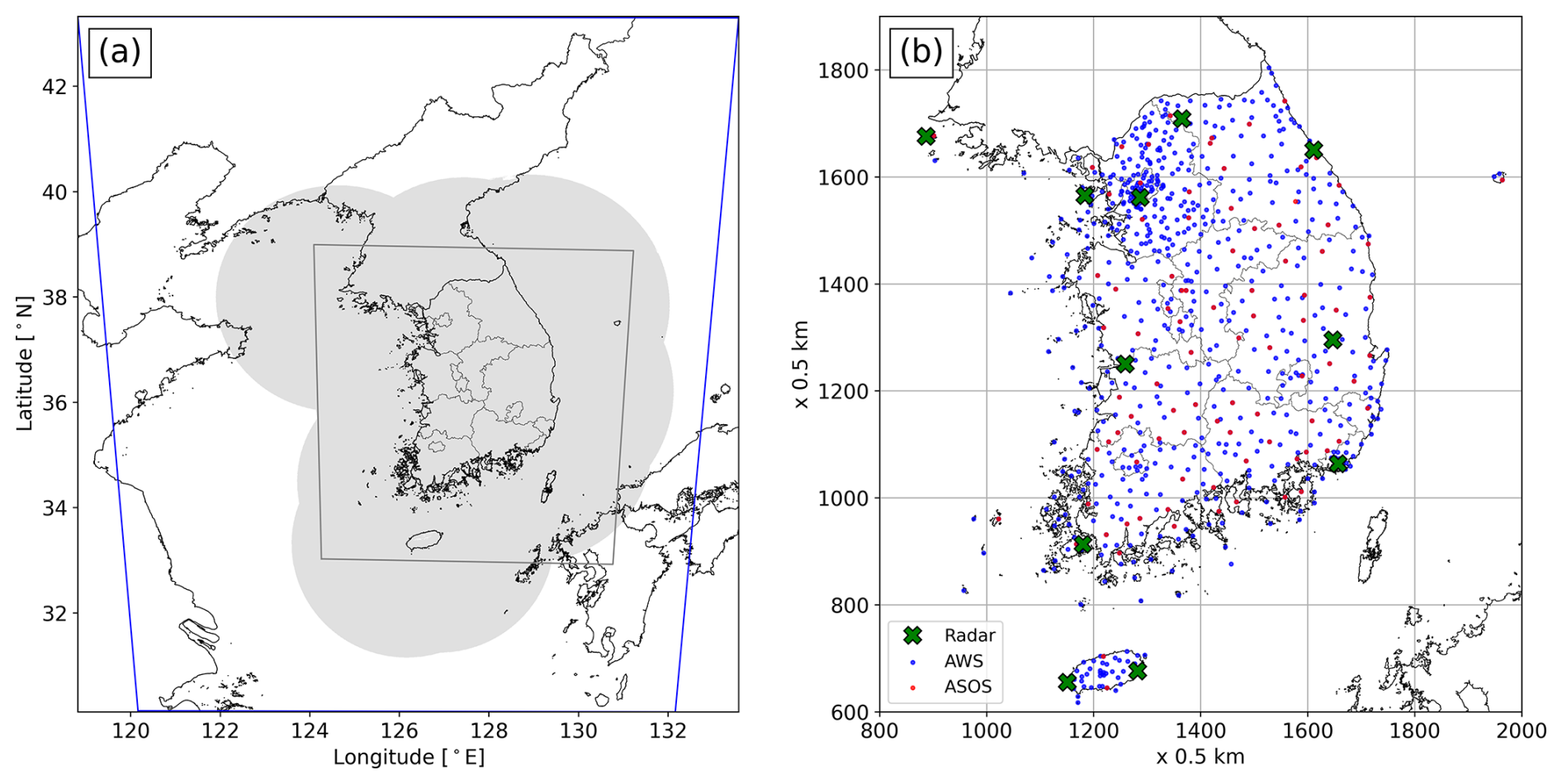
Figure 1 (a) Radar observation domains. The blue outline shows the HSR domain provided through the KMA API Hub at 0.5 km resolution (2305 pixels × 2881 pixels). The gray-shaded area denotes the nationwide HSR radar composite coverage, and the inner gray line indicates the verification domain. (b) Enlarged view of the verification domain, showing the locations of weather radars (green crosses), automatic weather systems (AWSs; blue dots), and automated synoptic observing systems (ASOSs; red dots).

Single-radar HSR fields from 11 weather radars operated by KMA (10 S-band and 1 C-band) are mosaicked to produce the nationwide composite reflectivity product. Table B1 (Appendix B) summarizes the operation start year, the year of dual-polarization upgrade, antenna altitude, and frequency band for each radar site. Most radars were sequentially upgraded to dual-polarization systems between 2014 and 2019, with Baengnyeongdo being the first (2014) and Gangneung the last (2019) among the ten operational sites, consistent with KMA's nationwide upgrade schedule. The Incheon International Airport radar was separately replaced with a dual-polarization system in August 2022. As a result, radar hardware configurations changed during the study period. In addition, operational scanning strategies, and consequently compositing altitude selection and quality control procedures, may have evolved over time. Although the HSR composite is generated within a standardized framework, potential impacts of these changes on long-term reflectivity homogeneity cannot be fully excluded.

Figure 1 illustrates the radar domains and their locations used in this study. The blue outline denotes the fixed 500 m grid domain provided through the KMA API Hub and used for generating the merged radar–gauge precipitation fields. The gray-shaded area indicates the representative spatial coverage of the HSR composite. Although this coverage is not strictly constant over the 9-year period due to changes in radar operation and network configuration, it represents the typical extent of nationwide radar coverage. Temporary radar outages and maintenance periods are reflected in the operational HSR composite product. No additional spatial gap filling or correction was applied to the radar data prior to merging. Reflectivity was converted to rainfall intensity using the operational Z–R relationship adopted by KMA (see Sect. 3.2, Eq. 1) before the radar–gauge merging procedure.

2.2 KMA rain gauge data

Rainfall observations were obtained from two nationwide automatic observation networks operated by the Korea Meteorological Administration (KMA): the Automatic Weather System (AWS) and the Automated Synoptic Observing System (ASOS). As of 2023, the combined network consists of approximately 550 AWS stations and 100 ASOS stations (Fig. 1b) across South Korea, corresponding to an average inter-station spacing of approximately 13 km. AWS stations are primarily installed in mountainous and rural areas to monitor localized weather conditions and are equipped with tipping-bucket rain gauges with a resolution of 0.5 mm per tip. ASOS stations are located at principal meteorological sites and follow World Meteorological Organization (WMO) standards, using weighing-type gauges with a measurement resolution of 0.1 mm. Both networks provide rainfall observations at 1 min temporal resolution, with precipitation amounts recorded in millimeters (mm).

The 1 min rainfall time series were subjected to quality control procedures prior to merging. These procedures included the detection of missing values, removal of physically unrealistic intensities, and identification of abrupt resets in cumulative tipping-bucket measurements (WMO, 2018). Records failing these checks were excluded from further analysis. The quality-controlled 1 min data were then aggregated into 10 min accumulations to reduce short-term variability and measurement noise. These accumulations were subsequently converted to rainfall intensity (mm h⁻¹) and used as gauge input for the radar–gauge merging procedure.

Figure 2 Overall workflow of the RRBF-based radar-gauge merging procedure.

3 Methodology

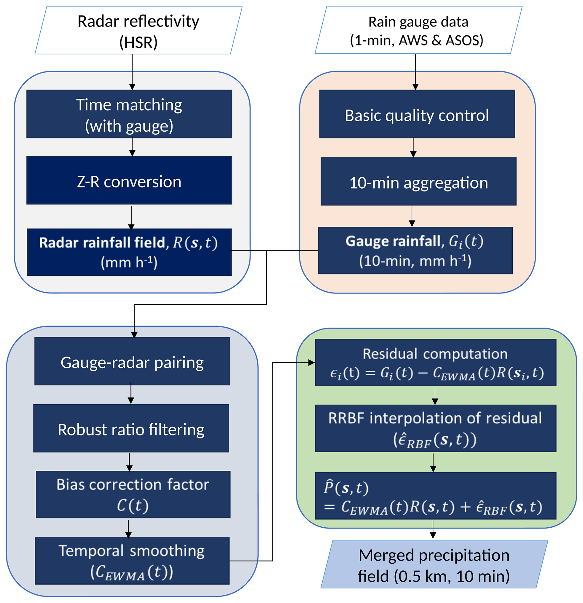
This section describes the radar–gauge merging procedure used to generate the high-resolution precipitation dataset. The processing framework is designed to ensure temporal consistency and spatial representativeness while integrating radar and rain gauge observations. Figure 2 provides an overview of the workflow, including gauge preprocessing, radar rainfall estimation, temporally constrained bias correction, residual interpolation using the RRBF method, and validation. In this study, R(s,t) denotes the radar-derived rainfall field at location s and time t, while G_i(t) denote the 10 min rainfall observed at the ith rain gauge. The radar rainfall corresponding to the ith gauge is denoted by R(s_i,t). The bias correction factor and its temporally smoothed value are denoted by C(t) and C_EWMA(t), respectively.

3.1 Gauge data processing

Rain gauge observations from the AWS and ASOS networks were subjected to basic quality control prior to merging. Missing values were identified, and range checks were applied to exclude unrealistic rainfall intensities exceeding 8 mm min⁻¹ (El Hachem et al., 2022). Following Ryu et al. (2025), the quality-controlled 1 min rainfall data were aggregated into 10 min accumulations (that is, 10 min average rainfall rate) to reduce short-term variability. These average rainfall rates were used as gauge input for the radar–gauge merging procedure.

3.1.1 Radar rainfall estimation

Radar reflectivity from the nationwide HSR composite was converted to rainfall intensity using the operational Z–R relationship adopted by KMA:

$$\begin{array}{}\text{(1)}& Z=\mathrm{148}{R}^{\mathrm{1.59}},\end{array}$$

as reported by Ro et al. (2022). Radar–gauge temporal matching followed the procedure described in Ryu et al. (2025). For each 10 min radar time step, gauge rainfall was accumulated over the corresponding 10 min period ending 8 min after the radar observation time and then converted to rainfall intensity (mm h⁻¹). A minimum rainfall threshold of 0.1 mm h⁻¹ was applied uniformly to both radar and gauge data across all temporal aggregations, and values below this threshold were treated as no-rain. This value corresponds to the finest resolvable rainfall rate achievable with ASOS gauges (0.1 mm) when accumulated over 60 min window. For 10 min accumulation, the same nominal threshold was retained for consistency; in this case the minimum non-zero rainfall rate that any gauge in the network can physically report is higher (0.6 mm h⁻¹ for ASOS and 3.0 mm h⁻¹ for AWS, owing to their respective tipping/weighing resolutions), so that the 0.1 mm h⁻¹ threshold functions equivalently to a strictly non-zero criterion at this timescale.

3.1.2 Estimation of temporally consistent bias correction factor

Radar rainfall at each gauge location was extracted from the nearest grid cell. To reduce representativeness differences between point-scale gauge measurements and gridded radar data, radar rainfall was averaged over a 3 pixels × 3 pixels window (1.5 km × 1.5 km) centered on each station.

Bias correction factors were estimated only when both radar and gauge rainfall exceeded 0.5 mm h⁻¹ and when at least 20 valid gauge–radar pairs were available. Individual ratios were calculated as

$$\begin{array}{}\text{(2)}& q_i\left(t\right)={\displaystyle \frac{G_i\left(t\right)}{R_i\left(t\right)}},\end{array}$$

where G_i(t) and R_i(t) denote gauge and radar rainfall at station i and time t, respectively. Ratios outside the 5th–95th percentile range were excluded to limit the influence of outliers. The raw bias correction factor was defined as

$$\begin{array}{}\text{(3)}& C\left(t\right)={\displaystyle \frac{{\sum }_{i=\mathrm{1}}^N{G}_i\left(t\right)}{{\sum }_{i=\mathrm{1}}^N{R}_i\left(t\right)}},\end{array}$$

where N is the number of valid pairs. To reduce abrupt temporal variability, changes in C(t) relative to the previous time step were limited to ± 30 %. The final correction factor was obtained using an exponentially weighted moving average (EWMA; Hunter, 1986):

$$\begin{array}{}\text{(4)}& C_{\text{EWMA}}\left(t\right)=\mathit{\alpha }C\left(t\right)+(\mathrm{1}-\mathit{\alpha })C_{\text{EWMA}}(t-\mathrm{1}),\mathit{\alpha }=\mathrm{0.5}.\end{array}$$

If fewer than 20 valid pairs were available, the correction factor from the previous time step was retained.

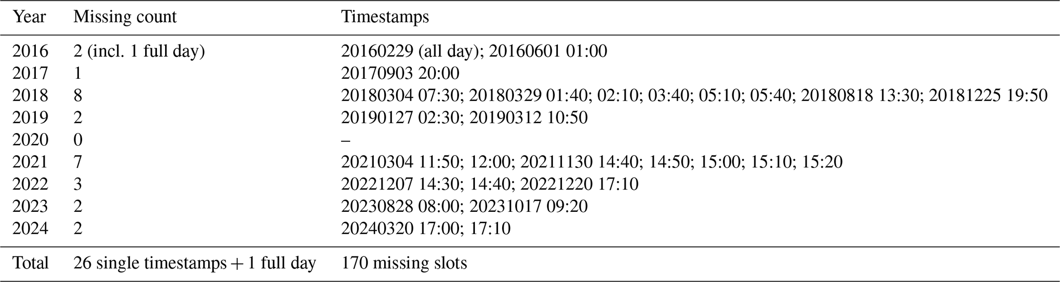
Table 1 Summary of missing 10 min RRBF precipitation timestamps (2016–2024). All time stamps are reported in Local Standard time (KST, UTC + +9).

3.1.3 RRBF based residual interpolation

After bias correction, residuals between gauge observations and corrected radar rainfall were computed as

$$\begin{array}{}\text{(5)}& {\mathit{ϵ}}_i\left(t\right)=G_i\left(t\right)-C_{\text{EWMA}}\left(t\right)R_i\left(t\right).\end{array}$$

Residual interpolation was performed only when at least five stations satisfied the rainfall threshold (≥ 0.5 mm h⁻¹ for both radar and gauge observations). The residuals were interpolated at an arbitrary location z using a radial basis function (RBF) approach (Buhmann, 2003; Fasshauer, 2007; Ryu et al., 2025):

$$\begin{array}{}\text{(6)}& {\widehat{\mathit{ϵ}}}_{\text{RBF}}(z,t)={\sum }_{i=\mathrm{1}}^N{w}_i\left(t\right)\mathit{\varphi }(\mathrm{|}z-z_i\mathrm{|}).\end{array}$$

Here, an exponential RBF kernel was adopted, defined as $\mathit{\varphi }(\mathrm{|}\cdot \mathrm{|})=\text{exp}(-\mathrm{|}\cdot \mathrm{|}/s)$, with a shape parameter of s = 16 km (Ryu et al., 2024). When fewer than five stations satisfied the threshold, residual interpolation was omitted, and only the bias-corrected radar rainfall was retained. The final merged precipitation field was defined as

$$\begin{array}{}\text{(7)}& \widehat{P}(z,t)=C_{\text{EWMA}}R(z,t)+{\widehat{\mathit{ϵ}}}_{\text{RBF}}(z,t).\end{array}$$

3.2 Validation strategy

The merged precipitation fields were evaluated using a leave-one-out cross-validation (LOOCV) approach applied to the RRBF residual interpolation. At each time step, individual stations were sequentially excluded, and residuals at the excluded locations were estimated using the remaining stations. To reduce computational cost, LOOCV errors were calculated using Rippa's theorem (Rippa, 1999), which allows efficient estimation of cross-validation errors without recomputing the interpolation for each station. Note that the excluded station was withheld only from the residual interpolation; it was retained in the estimation of the domain-wide bias factor C(t) and hence of C_EWMA, so the validation is not fully independent of the gauge observations. Because C(t) is estimated from a large number of gauge-radar pairs after outlier filtering and is temporally constrained and smoothed, the contribution of a single station is expected to be small. Nevertheless, the LOOCV statistics should be regarded as slightly optimistic. Validation metrics included mean absolute error (MAE), normalized mean absolute error (NMAE), normalized bias error (NBE), and the Pearson correlation coefficient (COR).

4 Description of the released dataset

4.1 Overview of temporal coverage

The dataset is a nationwide radar–gauge merged precipitation product covering the period from 1 January 2016 to 31 December 2024. Precipitation fields are provided at 10 min intervals with a spatial resolution of 0.5 km on a regular grid consistent with the KMA HSR composite domain. The dataset is generated using the RRBF-based merging framework described in Sect. 3 and provides spatially continuous precipitation estimates over South Korea.

4.2 Temporal completeness and missing data

A total of 473 472 10 min intervals are expected over the 9-year period. Among these, 170 time steps (0.036 %) are missing due to unavailable or empty radar input files in the operational HSR archive. Most missing cases correspond to isolated single time steps. The only extended data gap occurred on 29 February 2016, when the national radar composite was unavailable for the entire day. No temporal interpolation or gap filling was applied to replace missing intervals. A complete list of missing timestamps is provided in Table 1.

4.3 File naming convention and data format

The dataset is stored as individual NetCDF files, each corresponding to a 10 min average precipitation field. File names follow the convention Radar_Gauge_RRBF_YYYYMMDDHHmm.nc, where YYYYMMDDHHmm denotes the timestamp in Local Standard Time (KST, UTC + 9). The files are organized in a hierarchical directory structure by month and day, following the format YYYYMM/DD/Radar_Gauge_RRBF_YYYYMMDDHHmm.nc, where YYYYMM represents the year and month and DD represents the day of the month. For data distribution, each monthly directory (YYYYMM) is archived as a compressed file named YYYYMM.tar.gz.

Within each file, precipitation is stored on a regular Lambert Conformal Conic (LCC) projected grid with a spatial resolution of 0.5 km. The grid consists of 2305 points × 2881 points in the east–west and north–south directions, respectively, consistent with the operational HSR radar grid provided by KMA. Each NetCDF file contains a single precipitation field corresponding to the observation time. Projection parameters and coordinate variables are defined in accordance with CF metadata conventions. All files are stored in NetCDF4 format with internal compression to reduce storage requirements while preserving data integrity.

4.4 Variables and metadata

The primary variable (RR) represents the merged precipitation field expressed as rainfall intensity (mm h⁻¹). The values correspond to 10 min averages expressed as equivalent hourly rates. Data are stored as scaled 16-bit integers with a scale factor of 0.1. Each file also includes the temporally smoothed radar–gauge bias correction factor (C_EWMA), stored as a one-dimensional variable along the time dimension. Global attributes provide information on spatial resolution, projection parameters, temporal coverage, data sources, and processing history. All variables and metadata follow CF-compliant NetCDF conventions to facilitate interoperability and long-term reuse.

This per-interval file structure reflects the near-real-time production design of the RRBF framework, in which each precipitation field is generated and made available as soon as processing is completed. A comparable practice is followed by KMA, which distributes its operational composite radar reflectivity product (HSR) as individual files at 5 min intervals. Since one objective of this dataset is to support future operational implementation, the per-interval structure was preserved to reflect the native output of the processing algorithm. For archival distribution, however, individual files are aggregated into monthly compressed archives to reduce the total file count and facilitate data transfer (see Sect. 6).

5 Results

5.1 Event-based evaluation of the radar–gauge merging method (summer 2022)

The performance of the RRBF-based merging framework was evaluated using rainfall events observed from June to August 2022 over South Korea. This period includes both convective and stratiform precipitation associated with the East Asian summer monsoon. Only time steps with 10 min gauge rainfall rate greater than or equal to 0.1 mm h⁻¹ were included in the analysis. Two types of temporal accumulation windows (10 min and 1 h) were used for cross-validation.

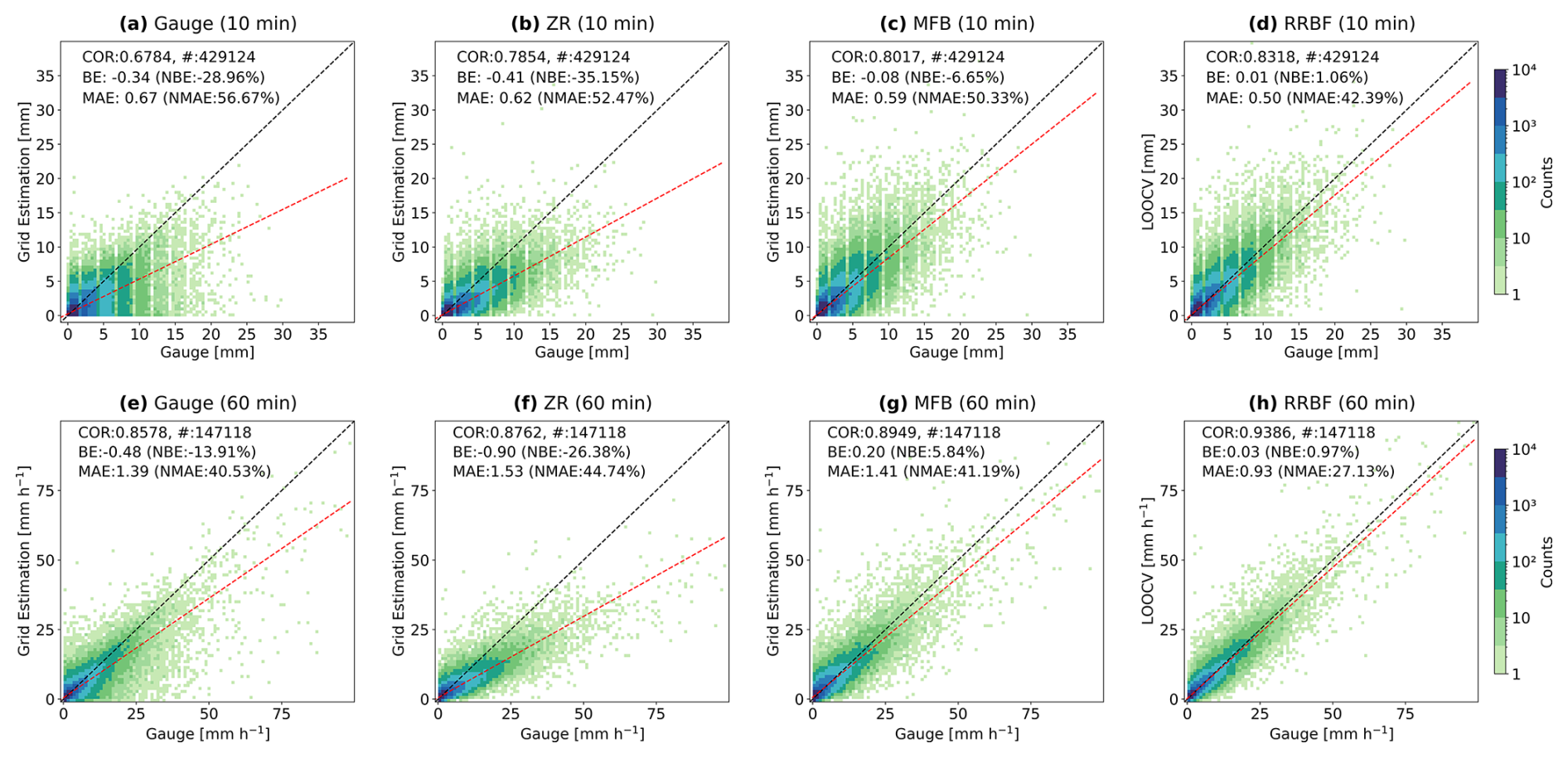
Figure 3 Scatter density plots comparing gauge interpolation, radar-only Z–R, mean field bias (MFB), and RRBF-merged precipitation estimates with rain gauge observations for summer rainfall events (June–August 2022). Panels (a)–(d) show 10 min accumulated rainfall (mm). Panels (e)–(h) show non-overlapping 60 min accumulated rainfall (mm) obtained by summing six consecutive 10 min accumulations. The dashed black line indicates the 1:1 relationship, and the red dashed line represents the linear regression fit.

5.1.1 Comparison of estimated accuracy against rain gauges

Figure 3 presents scatter density plots comparing estimated rainfall with rain gauge observations for summer 2022 events. Figure 3a–d show 10 min accumulated rainfall (mm). Figure 3e–h show non-overlapping 60 min accumulated rainfall obtained by summing six consecutive 10 min accumulations from the 10 min time series; these windows are not necessarily aligned to the top of the clock hour. For reference (Fig. 3a and e), gauge-only rainfall fields were obtained by interpolating gauge observations using the RBF method. Radar-only estimates based on the operational Z–R relationship and mean field bias (MFB) adjustment are shown in Fig. 3b, c and f, g, respectively. The RRBF results (Fig. 3d and h) correspond to LOOCV estimates, ensuring independence between validation observations and interpolation inputs.

For rainfall intensities derived from 10 min accumulations (Fig. 3a–d), the Z–R estimates exhibit a negative bias (NBE = −35.15 %) and relatively large dispersion (COR = 0.7854; MAE = 0.62 mm). The MFB adjustment reduces the bias (NBE = −6.65 %) but still shows considerable scatter around the 1:1 line. The RRBF method demonstrates higher correlation (COR = 0.8318) and lower MAE (0.50 mm), with near-zero bias (NBE = 1.06 %). The discrete banding patterns visible in the scatter plots, particularly along the x-axis, arise from the finite resolution of tipping-bucket rain gauges. Rainfall is recorded in discrete increments (e.g., 0.5 mm), resulting in quantized 10 min accumulations that produce distinct linear patterns in the scatter distribution.

For the 60 min accumulated rainfall (Fig. 3e–h), all methods show improved agreement due to temporal aggregation. The RRBF method achieves the highest correlation (COR = 0.9386) and lowest MAE (0.93 mm h⁻¹), compared to the Z–R (COR = 0.8762; MAE = 1.53 mm h⁻¹) and MFB (COR = 0.8949; MAE = 1.41 mm h⁻¹) estimates.

Across both temporal aggregation approaches, the RRBF-based merging approach shows reduced bias and improved agreement with rain gauge observations relative to radar-only estimates. These results indicate that the RRBF framework provides consistent performance across different temporal scales.

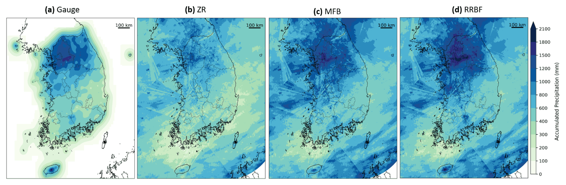
Figure 4 Spatial distribution of accumulated precipitation (mm) from June to August 2022 derived using different estimation methods: (a) gauge-based RBF interpolation, (b) radar-only Z–R product, (c) mean field bias (MFB)–corrected radar rainfall, and (d) RRBF-based merged precipitation. The dashed contours indicate regions where the 3-month accumulated precipitation derived from gauge-only RBF interpolation exceeds 100 mm, representing areas with substantial gauge influence. All panels are shown over the same spatial domain.

5.1.2 Spatial characteristics of accumulated precipitation

Figure 4 presents the spatial distribution of accumulated precipitation from June to August 2022 derived using different estimation methods. Figure 4a shows the gauge-based precipitation field obtained by applying radial basis function (RBF) interpolation to rain gauge observations, while Fig. 4b–d show the corresponding accumulations from the radar-only Z–R product, the mean field bias (MFB) – corrected field, and the RRBF-based merged field, respectively.

The gauge-based RBF interpolation (Fig. 4a) reproduces localized rainfall maxima associated with summer precipitation but exhibits spatial smoothing and pronounced gradients in regions with sparse station coverage. The dashed contours indicate areas where the 3-month accumulated precipitation exceeds 100 mm based on the gauge-only RBF field. This threshold is used as a practical criterion to identify regions with substantial seasonal rainfall and strong gauge influence and does not represent a physical boundary. Outside these regions, spatial uncertainty increases due to limited station density.

The radar-only Z–R product (Fig. 4b) captures the large-scale precipitation patterns over the Korean Peninsula but shows lower accumulated amounts in regions influenced by intense convective rainfall compared to the gauge-based field. The MFB-corrected field (Fig. 4c) reduces the overall differences in accumulated precipitation relative to the Z–R product; however, its spatially uniform adjustment results in residual spatial discrepancies.

The RRBF-based merged field (Fig. 4d) preserves the large-scale spatial structure of radar-derived precipitation while incorporating gauge-based adjustments. The resulting accumulation patterns show closer agreement with the gauge-based field in regions with dense gauge coverage. When precipitation is accumulated over the full 3-month period, azimuthal spatial features associated with radar beam geometry and scanning characteristics remain evident (Fig. 4b and c). These artifacts originate from the HSR compositing process and therefore should be addressed within the radar processing stage. Although residual interpolation partially reduces these features, they are not fully eliminated.

5.2 Long-term validation (2016–2024)

To assess the long-term characteristics of the merged precipitation dataset, analyses were conducted over the full period from 2016 to 2024. The evaluation focuses on interannual variability and the spatial distribution of accumulated precipitation.

5.2.1 Interannual variability and accumulated precipitation

Annual accumulated precipitation was calculated for each year from 2016 to 2024 using the RRBF-based merged dataset. Annual totals were spatially averaged within the dashed region shown in Fig. 4, which represents an area with sufficiently dense gauge observations to ensure a consistent influence on the merged field and defines the analysis domain for interannual comparison.

Figure 5 presents the time series of annual mean precipitation over this domain. Pronounced interannual variability is evident throughout the 9-year period. Among the analyzed years, 2017 exhibits the lowest annual precipitation, whereas 2020 records the highest total, reflecting year-to-year differences in precipitation conditions. Despite these variations, the dataset exhibits temporally consistent behavior without abrupt discontinuities. The time series indicates that interannual variability is robustly preserved across the full record from 2016 to 2024.

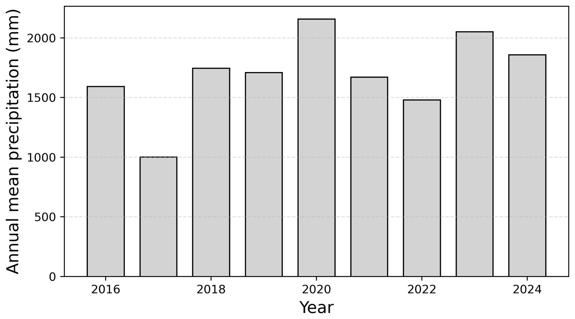
Figure 5 Time series of annual mean precipitation averaged over the analysis domain for 2016–2024.

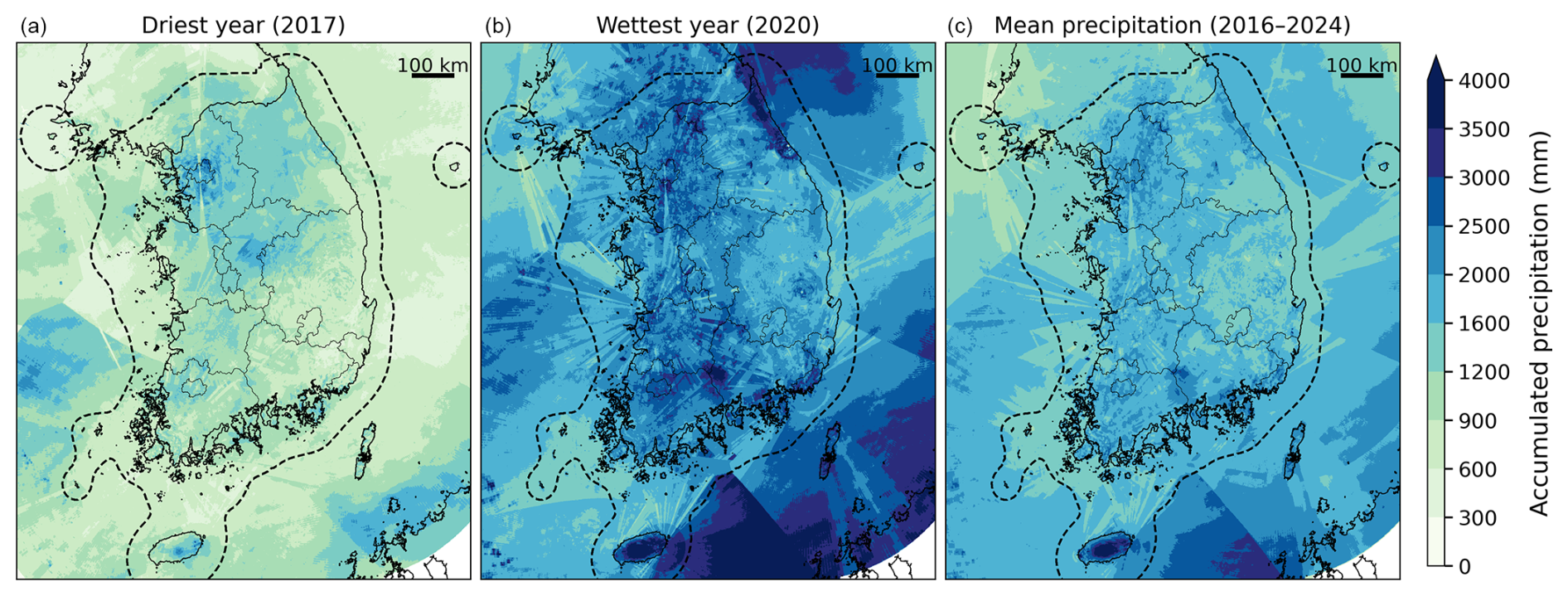
Figure 6 Spatial distribution of annual accumulated precipitation derived from the RRBF-based merged dataset for (a) 2017 (driest year), (b) 2020 (wettest year), and (c) the 9-year mean (2016–2024). The dashed outline denotes the analysis domain used for interannual statistics.

Figure 6 shows the spatial distribution of annual accumulated precipitation for the driest year (2017), the wettest year (2020), and the 9-year mean over the period 2016–2024. The dashed boundary denotes the analysis domain used for the statistical evaluation presented in Fig. 5. 2020 exhibits substantially higher annual precipitation over widespread areas, together with pronounced spatial variability, particularly over the southern and eastern parts of the peninsula. This spatial structure is likely associated with a combination of the exceptionally prolonged summer rainy season, orographic and coastal effects, and heavy rainfall from successive typhoons in late August and early September. In particular, Typhoons Maysak and Haishen produced substantial rainfall over southern and eastern Korea, including the mountainous regions of Gangwon Province (KMA National Typhoon Center, 2021), which may have contributed to the enhanced spatial structure observed in the 2020 annual accumulation field. The 9-year mean field represents the average spatial distribution of precipitation during the study period and shows relatively persistent localized maxima associated with orographic and coastal influences.

Compared to event-scale precipitation fields derived from short-term summer events, annual and multi-year accumulations exhibit substantially smoother spatial patterns. This smoothing reduces the apparent impact of short-term variability and radar observation artifacts. However, weak spatial signatures related to radar beam geometry are still detectable in some areas, indicating that residual structural artifacts of radar observations persist even in long-term accumulations. It should be noted that Fig. 6 presents only the sub-domain used for statistical analysis. The full dataset is available over the complete radar composite domain (2305 × 2881 grid points) shown in Fig. 1a. Annual accumulation maps for all individual years over the full domain are provided in Appendix A.

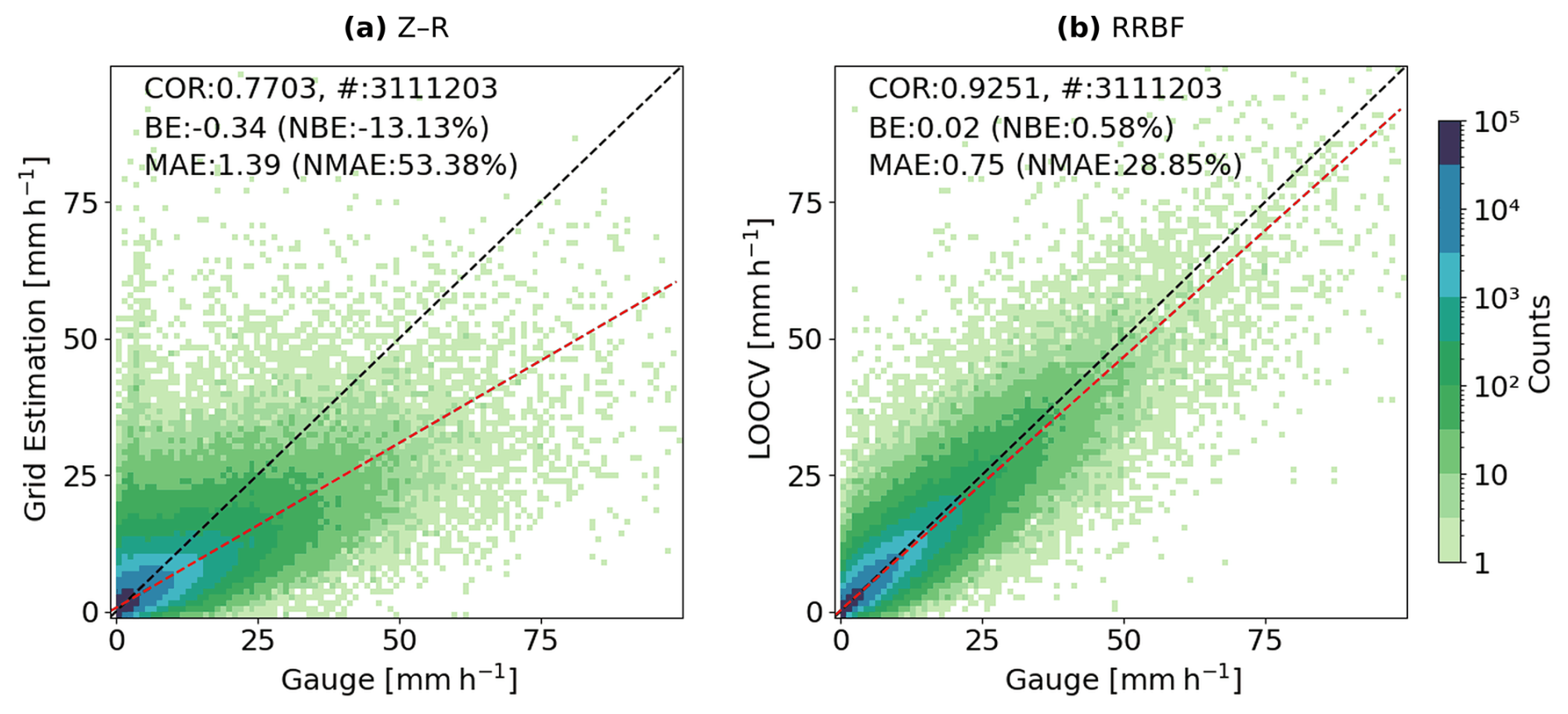
Figure 7 Scatter density plots of hourly precipitation comparing (a) radar-only Z–R estimates and (b) RRBF-based merged precipitation against rain gauge observations for the period 2016–2024. Only cases with gauge-observed rainfall greater than 0.1 mm h⁻¹ are included. Radar precipitation values are extracted from the grid cell closest to each gauge location, whereas RRBF estimates correspond to LOOCV results. Dashed lines indicate the 1:1 relationship, and colors represent the logarithm of sample density.

5.2.2 Validation against rain gauge observation

The long-term statistical performance of the merged precipitation dataset was evaluated against KMA rain gauge observations over the period 2016–2024 at an hourly time scale, using non-overlapping 60 min accumulated rainfall derived by summing six consecutive 10 min observations, with windows not necessarily aligned to the top of the clock hour. Radar-only Z–R precipitation and RRBF-based merged precipitation were compared across multiple rainfall intensity thresholds. Figure 7 presents scatter density plots for cases with gauge-observed rainfall ≥ 0.1 mm h⁻¹. Radar-only values were obtained from the nearest radar grid cell at each gauge location, whereas RRBF values correspond to LOOCV estimates, ensuring independence between validation observations and interpolation inputs.

Table 2 Statistical comparison of hourly radar-only Z–R and RRBF precipitation against KMA rain gauge observations for 2016–2024 at multiple rainfall thresholds.

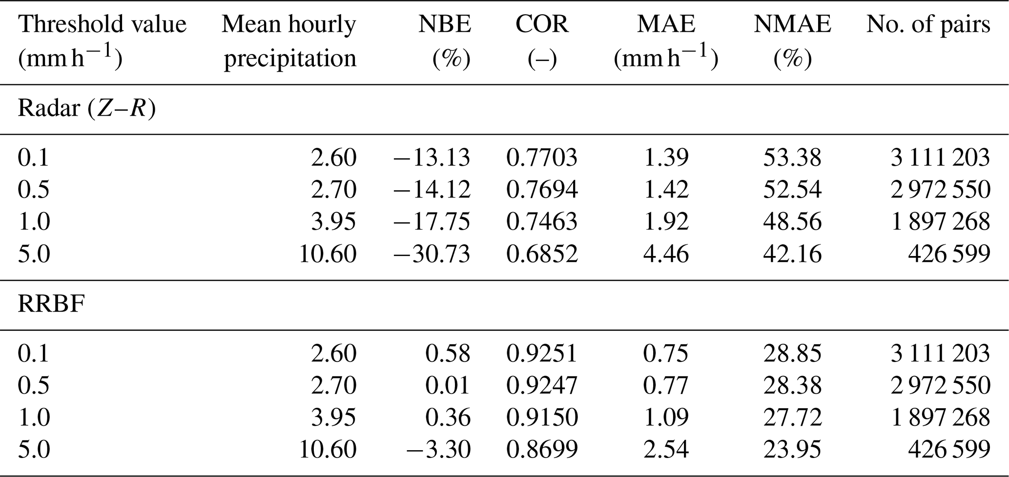
Consistent with the event-based analysis, the Z–R estimates exhibit a systematic negative bias across the full range of observed intensities, with increasing dispersion at higher rainfall rates. Moreover, the long-term evaluation demonstrates that these error characteristics persist across the entire analysis period. In contrast, the RRBF estimates show a sustained reduction in bias and improved agreement with gauge observations over all intensity ranges. For rainfall ≥ 0.1 mm h⁻¹, the normalized mean absolute error (NMAE) decreases from 53.38 % (Z–R) to 28.85 % (RRBF), while the correlation coefficient increases from 0.7703 to 0.9251 (Table 2). The bias is also markedly reduced, from −13.13 % to 0.58 %.

Table 2 summarizes performance metrics for rainfall thresholds of 0.1, 0.5, 1.0, and 5.0 mm h⁻¹. Across all thresholds, the RRBF-based estimates consistently demonstrate improved performance relative to radar-only Z–R estimates, indicating that the benefits observed in event-scale analysis are robust across long-term conditions. As the threshold increases, the negative bias of the Z–R estimates becomes progressively larger (NBE from −13.13 % to −30.73 %) and their correlation with gauge observations decreases (COR from 0.7703 to 0.6852), reflecting the tendency of radar-only estimates to underestimate more heavily during higher-intensity rainfall. In contrast, the RRBF estimates maintain a bias close to zero across all thresholds (NBE within ± 3.3 %) and show only a modest decline in correlation (COR from 0.9251 to 0.8699), indicating that the gauge-based bias correction remains effective even for higher rainfall intensities.

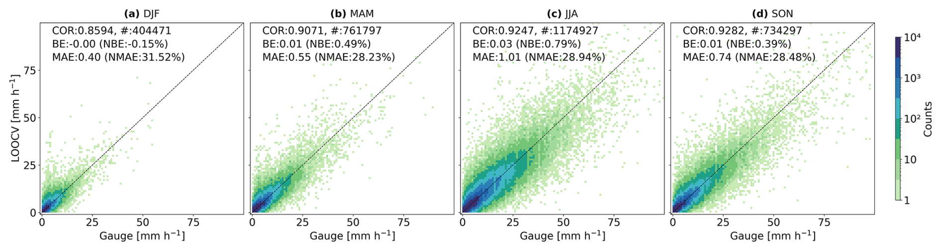
Figure 8 Seasonal scatter density plots of RRBF-based LOOCV precipitation estimates against rain gauge observations for (a) DJF, (b) MAM, (c) JJA, and (d) SON during the period 2016–2024. Colors denote the logarithm of sample density, and dashed lines indicate the 1:1 relationship. Performance statistics shown in each panel summarize seasonal variations in bias and correlation.

Seasonal variations in the performance of the RRBF-based precipitation estimates are presented in Fig. 8 for winter (December–February, DJF), spring (March–May, MAM), summer (June–August, JJA), and autumn (September–November, SON). The correlation coefficient ranges from approximately 0.86 in DJF to values exceeding 0.92 in JJA and SON. A relatively larger dispersion is evident during winter, whereas warm-season estimates show tighter clustering around the 1:1 reference line.

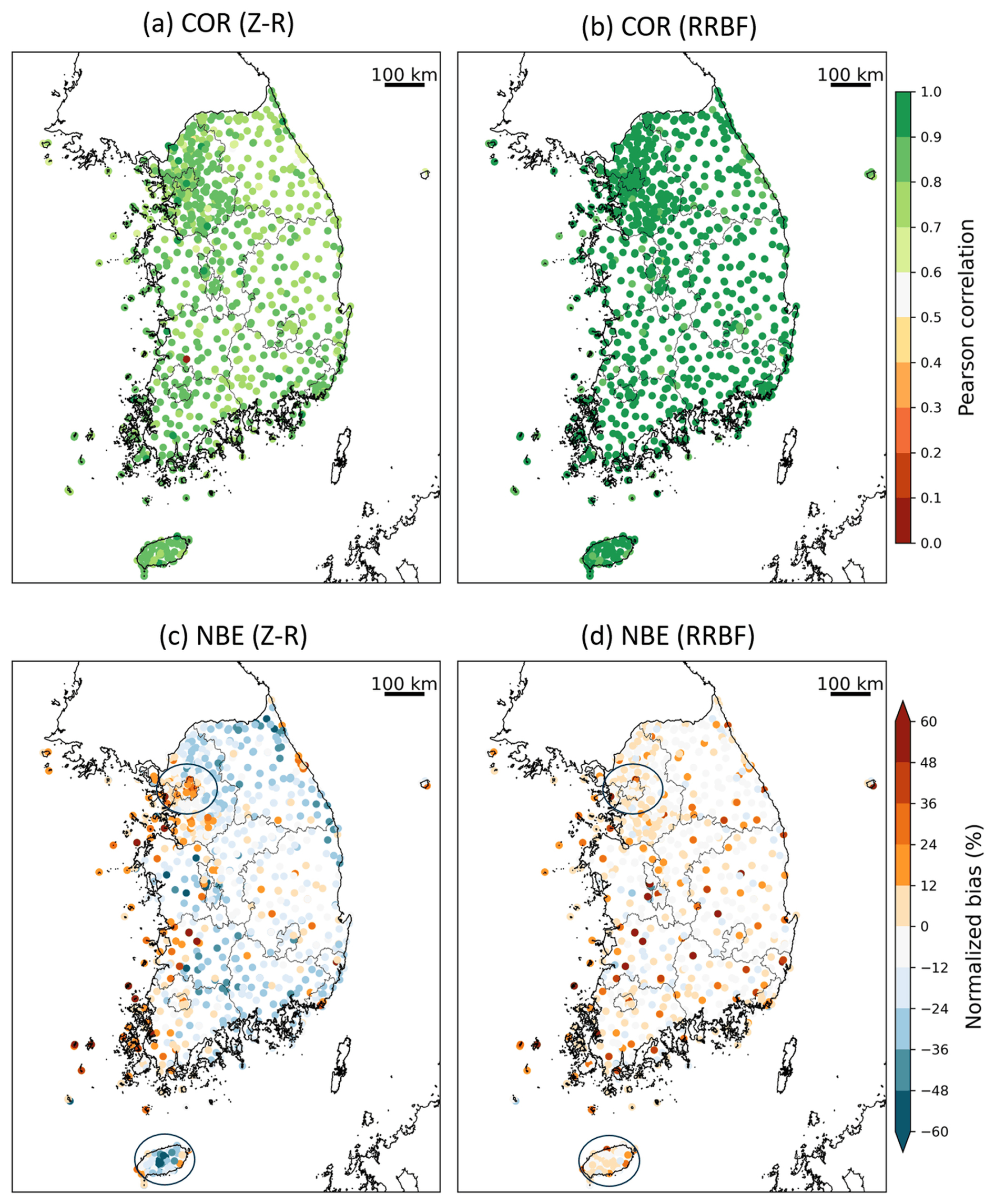
Figure 9 Station-based spatial distributions of Pearson correlation coefficient (COR) and normalized bias error (NBE) for radar-only Z–R (a, c) and RRBF-based precipitation (b, d) over South Korea during 2016–2024. RRBF statistics are derived from leave-one-out cross-validation (LOOCV) estimates.

5.2.3 Spatial error distributions

To assess the spatial characteristics of estimation performance, station-based COR and NBE were computed for each rain gauge over the period 2016–2024 using non-overlapping 60 min accumulated rainfall derived from 10 min data. Only hours with gauge-observed rainfall ≥ 0.5 mm h⁻¹ were included in the analysis. Figure 9 presents the spatial distribution of these metrics for radar-only Z–R estimates and RRBF-based precipitation. For the RRBF product, station-level statistics were derived from LOOCV estimates to ensure independence from the gauge observations used in the merging process.

For the radar-only Z–R estimates (Fig. 9a), correlation coefficients exhibit moderate to high values across South Korea, with pronounced spatial variability. Lower correlations are evident in some coastal regions and areas of complex terrain. In contrast, the RRBF-based estimates (Fig. 9b) show generally higher correlations at many stations and reduced spatial variability compared to the Z–R product.

The spatial distribution of normalized bias error further highlights differences between the two approaches. Radar-only Z–R estimates (Fig. 9c) are characterized by widespread negative bias across much of the domain, with spatially coherent underestimation in several regions, including coastal and mountainous areas. In the RRBF results (Fig. 9d), bias magnitudes are substantially reduced at many stations, and NBE values are more frequently centered near zero. Localized differences are apparent in regions such as the Seoul metropolitan area and Jeju Island, where bias patterns differ between the Z–R and RRBF estimates. On Jeju Island, this likely reflects beam blockage near Hallasan (1947 m, the highest mountain in South Korea), which requires the HSR algorithm to use higher-elevation scans and can lead to underestimation in the Z–R estimates; the RRBF estimates are less affected, as gauge observations are directly incorporated into the bias correction. Although some stations still exhibit relatively large positive or negative bias in the RRBF results, these are spatially isolated rather than regionally coherent. Overall, the station-based spatial analysis indicates that the RRBF-based precipitation estimates exhibit reduced bias magnitude and more spatially uniform correlation patterns compared to the radar-only Z–R estimates over the 2016–2024 period.

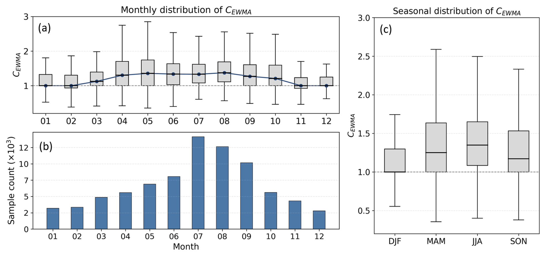
Figure 10 Monthly and seasonal distribution of C_EWMA for 2016–2024. (a) Monthly boxplots with blue markers indicating monthly means; the dashed line denotes C_EWMA=1. (b) Monthly sample counts (× 10³). (c) Seasonal boxplots grouped into DJF, MAM, JJA, and SON; the dashed line denotes C_EWMA=1.

5.2.4 Temporal distribution of the bias adjustment factor

To investigate the temporal characteristics of the radar–gauge adjustment, the distribution of C_EWMA was analyzed by month and season for the period 2016–2024 (Fig. 10). The correction factor C_EWMA represents the multiplicative bias adjustment factor applied to radar-derived precipitation; values greater than 1 indicate that radar estimates are, on average, lower than gauge observations. Figure 10a presents monthly boxplots of C_EWMA aggregated over the 9-year period. Median values exceed 1 in all months. Slightly higher medians are observed from late spring to summer (May–August), whereas winter months exhibit comparatively lower values. The interquartile range varies seasonally, with broader distributions during the warm season and narrower distributions in winter. Monthly sample counts (Fig. 10b) show a pronounced seasonal cycle, with substantially higher counts in July and August and lower counts during winter months. Months with larger sample sizes also tend to exhibit wider distributions of C_EWMA.

Seasonal boxplots (Fig. 10c) indicate that median values are lowest in DJF and higher in the other seasons. Variability also differs by season, with broader interquartile ranges in MAM and JJA and narrower distributions in DJF. These seasonal patterns reflect differences in both the magnitude and variability of the radar–gauge adjustment factor across seasons during 2016–2024.

6 Data availability

The radar–gauge merged precipitation dataset for South Korea (2016–2024) is publicly available on Zenodo:

• Part 1 (2016–2020):
  https://doi.org/10.5281/zenodo.19491708 (Ryu et al., 2026a)

• Part 2 (2021–2024):
  https://doi.org/10.5281/zenodo.19562910 (Ryu et al., 2026b).

The dataset was divided into two repositories owing to Zenodo's limits on the total number of files and total storage volume permitted per DOI, rather than for scientific reasons. Within each repository, the dataset is distributed as monthly compressed archives (YYYYMM.tar.gz), each containing NetCDF files for individual 10 min precipitation fields organized in the directory structure: “YYYYMM/DD/Radar_Gauge_RRBF_YYYYMMDDHHmm.nc”. Part 2 additionally includes supplementary information such as metadata describing missing data periods, the spatial domain (latitude–longitude grid definition), and a README file providing detailed guidance on data structure and usage. Radar input data were obtained from the KMA API Hub and are subject to KMA data policy. The merged dataset is released under the Creative Commons Attribution 4.0 International (CC BY 4.0) license.

7 Code availability

The processing code used to generate the dataset is not publicly available but may be provided by the corresponding author upon reasonable request.

8 Conclusions

This study presents a high-resolution radar–gauge merged precipitation dataset for South Korea covering the period 2016–2024. The dataset is provided at 0.5 km spatial resolution and 10 min temporal resolution and is based on nationwide composite radar reflectivity from the KMA and quality-controlled rain gauge observations from the AWS and ASOS networks. The merging framework combines a temporally smoothed multiplicative bias adjustment with residual interpolation using a radial basis function (RRBF). The bias correction factor is updated at 10 min intervals while incorporating information from previous time steps, and spatial discrepancies between radar and gauge observations are addressed through residual interpolation.

Event-based and long-term evaluations characterize the statistical, spatial, and seasonal performance of the merged dataset. Compared to radar-only Z–R estimates, the RRBF-based product exhibits reduced bias magnitude and higher correlation with rain gauge observations across rainfall thresholds and seasons. Station-based analyses further indicate more spatially uniform error characteristics relative to the radar-only product. The dataset captures interannual variability and spatial patterns of accumulated precipitation over 2016–2024. Seasonal variations in the bias adjustment factor reveal systematic differences in both magnitude and variability, consistent with seasonal rainfall characteristics.

Despite these improvements, limitations inherent to radar-based precipitation estimation remain, particularly in regions affected by complex terrain and partial radar beam blockage. In addition, rain gauge quality control in this study was based on general range checks and consistency filtering; site-specific measurement uncertainties and representativeness issues may contribute to localized residual discrepancies. Further refinement of gauge quality assurance procedures may help reduce these uncertainties in future developments.

The resulting dataset provides a continuous, high-resolution precipitation record for South Korea and is intended to support hydrological, climatological, and related applications requiring sub-hourly rainfall information. The dataset is publicly available and can support applications such as extreme rainfall analysis, hydrological modeling, and satellite precipitation validation. As one of the first long-term radar–gauge merged precipitation products at sub-kilometer and sub-hourly resolution for South Korea, this dataset represents a valuable resource for studies requiring detailed precipitation information.

Appendix A: Annual accumulated precipitation over the full composite domain (2016-2024)

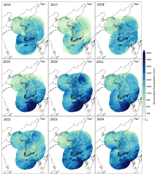
Figure A1 presents the spatial distribution of annual accumulated precipitation derived from the RRBF-based merged dataset for 2016–2024 over the full radar composite domain (2305 × 2881 grid points), corresponding to the area shown in Fig. 1a. In contrast to Fig. 6, which is limited to the sub-domain used for validation analysis (Fig. 1b), the maps in this appendix provide the complete spatial coverage of the dataset. The full set of annual accumulation maps is made available as part of the dataset accompanying this publication. These maps represent the full spatial extent of the precipitation dataset developed and provided in this study, illustrating its capability to capture large-scale precipitation patterns across the entire radar composite domain. The annual accumulation fields exhibit coherent large-scale spatial structures, with relatively higher precipitation along southern coastal regions and in mountainous areas. Interannual variability is also evident across the full domain, including comparatively dry conditions in 2017 and enhanced precipitation in 2020.

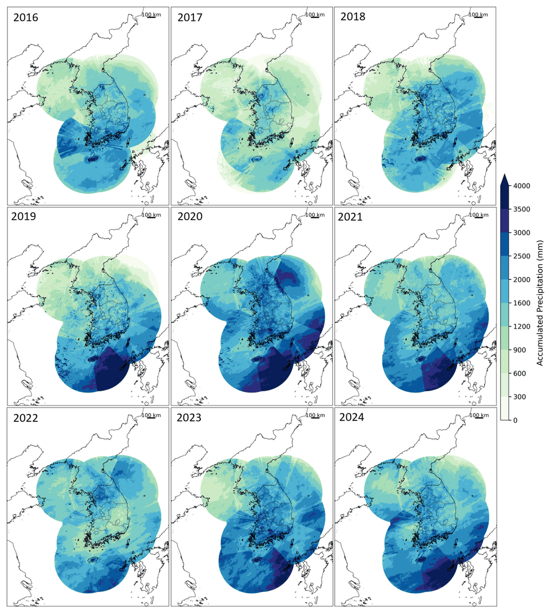
Figure A1 Annual accumulated precipitation (mm) over the full radar composite domain (2305 × 2881 grid points) for the period 2016–2024. The maps correspond to the operational HSR composite coverage shown in Fig. 1a and represent the complete spatial extent of the RRBF-based merged precipitation dataset developed in this study.

Appendix B: KMA weather radar site information

Table B1 summarizes the operation start year, the year of dual-polarization upgrade, antenna altitude, and frequency band for each radar site comprising the KMA composite network described in Sect. 2.1.

Table B1 Overview of the KMA weather radar network used to generate the HSR composite product, including operation start year, antenna altitude, dual-polarization upgrade year, and frequency band.

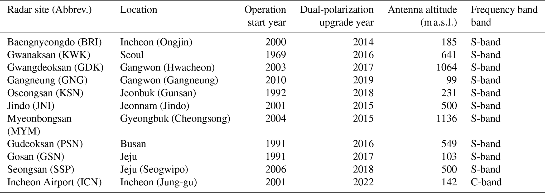
Source: KMA Weather Radar Center (2018); KMA API Hub (2025).