Global 30 m annual cropland extent dynamics (2000–2024): a harmonized baseline of structural evolution and regional disparities

Accurate annual information on cropland extent is essential for monitoring agricultural change, yet existing global products are often limited to snapshots or multiyear epochs and differ in their cropland definitions. Here we present GACED30, which, to our knowledge, is the first dedicated global 30 m annual cropland-extent dataset covering 2000–2024. The mapping framework combines gap-free SDC30 observations, spectral-semantic alignment of expert-annotated and spatially augmented samples, and rule-based spatial and temporal refinement. Independent classifiers were trained for each year using a common observation, feature, sample-construction, and modeling protocol, and the resulting annual record was used to derive pixel-level Cropping Frequency and 1 km Structural Evolution Indicators. Against independent stable-site FAST-Crop samples, GACED30 achieved an overall accuracy of 0.965 and an F₁ score of 0.844. Multitemporal assessments using GLAD Cropland and LUCAS reference samples showed higher recall and F₁ scores than GLC_FCS30D for both crop gain and crop loss, although the absolute transition scores remained modest. In a matched regional assessment in China, GACED30 achieved OA and F1 scores of 0.946 and 0.840, respectively, showing performance comparable with CACD. At the national scale, GACED30 agreed closely with definition-reconciled FAOSTAT statistics (R²: 0.95; area-weighted direction match rate: 83.1 %). The sample-adjusted global cropland area was estimated at 1488.5 Mha in 2024, approximately 30.0 Mha higher than in 2000. Persistent expansion was concentrated in parts of Africa and South America, whereas stability and reduction were more widespread across much of the Global North. GACED30 provides a harmonized baseline for monitoring global cropland-extent dynamics and is publicly available at https://doi.org/10.5281/zenodo.18199675 (Chen et al., 2026).

1 Introduction

Ensuring global food security while remaining within planetary boundaries is one of the defining challenges of the 21st century (Godfray et al., 2010; FAO, 2017). Rising food demand and climate variability intensify the tension between increasing agricultural production and limiting cropland encroachment into carbon-rich ecosystems and biodiversity hotspots (Tilman et al., 2011; Foley et al., 2011; Zhang et al., 2025b; Ceaușu et al., 2025). Assessing this trade-off requires moving from static measures of total area to the long-term spatiotemporal trajectories of agricultural expansion, stability, and reduction, here termed structural evolution (Potapov et al., 2022). Robust information on these long-term cropland dynamics is a foundational prerequisite for diagnosing the health of the global land system (Tu et al., 2024; FAO, 2025). By rigorously distinguishing between permanent land cover conversion (e.g., commodity-driven deforestation or urbanization) and the rotational variability inherent to management cycles, such data empowers policymakers to differentiate true sustainable intensification from extractive land reclamation (Tubiello et al., 2021; Pretty, 2018).

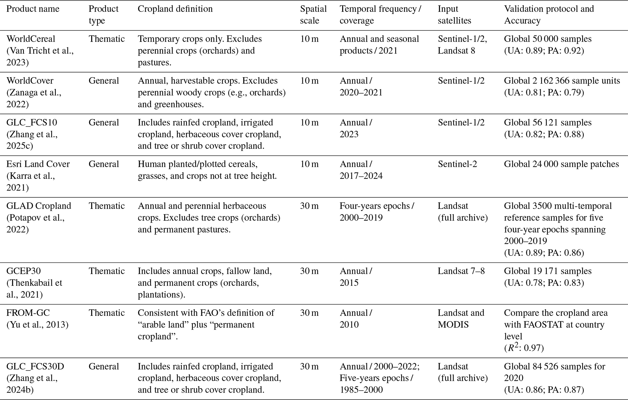
Global cropland monitoring has been transformed by the convergence of open satellite archives (Wulder et al., 2012; Drusch et al., 2012), machine learning (Zhu et al., 2017), and cloud computing (Gorelick et al., 2017), enabling a new generation of high-resolution (10–30 m) mapping products (Table 1). However, despite the emergence of high-resolution mapping products, current operational datasets exhibit critical limitations when applied to the monitoring of long-term structural evolution. These products generally fall into four categories, each constrained by specific trade-offs. The first two categories comprise short-term thematic studies (e.g., the 30 m GCEP30, Thenkabail et al., 2021, and 10 m WorldCereal, Van Tricht et al., 2023) and short-term comprehensive land cover products (e.g., ESA WorldCover, Zanaga et al., 2022, Esri Land Cover, Karra et al., 2021, and GLC_FCS10, Zhang et al., 2025c). While offering high spatial fidelity, these datasets function as independent temporal fragments or isolated snapshots. Lacking multi-decadal continuity, they cannot capture the historical trajectory required to distinguish current structural patterns from past land use dynamics. The third category involves long-term thematic products, represented by Global Land Analysis and Discovery (GLAD) Cropland (Potapov et al., 2022). While achieving high thematic accuracy, this dataset relies on multi-year epoch aggregation (e.g., 4-year composites) to mitigate observational gaps. Consequently, it primarily supports bi-temporal change detection (comparing aggregated epochs) rather than continuous annual monitoring. This aggregation strategy effectively blurs inter-annual dynamics, masking the exact timing of expansion or abandonment and limiting the ability to track detailed structural evolution. The fourth category consists of long-term comprehensive land cover products, such as GLC_FCS30D (Zhang et al., 2024b). Although offering a multi-decadal span (1985–2022), these generalist products frequently adopt broad definitions that encompass rainfed, herbaceous, and shrub-based mosaics, leading to systematic area overestimation (Tubiello et al., 2023b). Furthermore, their classification systems often fail to distinguish fallow-rotation cycles from natural vegetation changes. These semantic differences and temporal fluctuations complicate the robust identification of structural trends. Consequently, a gap remains for a global product that combines the thematic focus of a dedicated cropland map with annual coverage and a harmonized definition suitable for characterizing the long-term structural evolution of global agriculture.

Table 1 Summary of major global high-resolution (10 and 30 m) land cover products relevant to cropland monitoring.

The primary observational barrier to annual cropland mapping is the requirement for continuous, gap-free time series to capture the distinct intra-annual phenological pulse of agriculture. Unlike stable land cover types, the reliable separation of active cultivation from spectrally similar natural vegetation (e.g., grasslands) depends entirely on detecting the temporal signature of planting, green-up, and senescence (Bégué et al., 2018; Zhang et al., 2025a). However, preserving this high-frequency signal in optical satellite imagery is severely hampered by cloud contamination, which creates critical data gaps (Whitcraft et al., 2015). While strategies such as multi-year epoch aggregation (Potapov et al., 2022) effectively mitigate data gaps, they do so by sacrificing the annual temporal fidelity required to distinguish cropping cycles from natural variability. Consequently, recent advancements have shifted toward dense time-series reconstruction through sensor fusion – such as the Harmonized Landsat and Sentinel-2 (HLS) project (Claverie et al., 2018) and the generation of Seamless Data Cubes (SDC) (Chen et al., 2024; Liang et al., 2024; Liu et al., 2021).

Although gap-free observations provide the temporal continuity required for annual cropland monitoring, consistency also depends on the temporal and semantic compatibility of the training labels. Stable-classification theory suggests that classifiers can tolerate some random labeling errors during sample transfer (Gong et al., 2019, 2024), but systematic conflicts are more problematic, particularly where categories such as temporary grassland and fallow are defined differently across sample sources. In addition, the spectral similarity between temporary fallow and natural bare land can produce false negatives, spurious interannual variability, and biased long-term trends. Robust annual mapping therefore requires explicit spectral-semantic alignment and limited postclassification rules to reduce temporal and definition-level conflicts among heterogeneous training samples while preserving the cropland definition adopted by GACED30.

To address these challenges, we developed GACED30, to our knowledge the first dedicated global 30 m annual cropland-extent dataset spanning 2000–2024, using a harmonized mapping framework that integrates the gap-free 30 m Seamless Data Cube (SDC30) with spectral-semantic sample alignment and spatiotemporal refinement. The evaluation combined an independent FAST-Crop static thematic assessment, a multi-temporal endpoint-transition assessment using GLAD Cropland and European Union Land Use/Cover Area frame Survey (LUCAS) reference samples, a matched regional assessment in China, agro-ecological-zone-stratified performance diagnostics, sample-adjusted inter-product area comparison, and comparison with definition-reconciled FAOSTAT statistics. Leveraging this harmonized annual baseline, we quantified the long-term structural evolution of global agriculture. We derived a Cropping Frequency layer to characterize mapped cropland persistence and a 1 km Structural Trend Indicator to distinguish directional changes from interannual variability. This analysis reveals divergent agricultural trajectories between the expanding Global South and the stabilizing or contracting Global North, providing an evidence base for monitoring the changing footprint of global food systems. The dataset is publicly available at https://doi.org/10.5281/zenodo.18199675 (Chen et al., 2026).

The remainder of this paper is organized as follows: Sections 2 and 3 detail the datasets and the mapping framework; Sect. 4 presents the global, regional, and agro-ecological evaluation results, harmonization with agricultural statistics, and derived global cropping-frequency and structural-evolution patterns; and Sect. 5 discusses the product's advantages and limitations before concluding in Sect. 6.

2 Datasets

The generation and validation of the GACED30 dataset relied on a multi-faceted data strategy. This involved leveraging a high-density satellite data cube for primary analysis, incorporating auxiliary datasets for contextual information, utilizing extensive sample sets for model training and validation, and referencing global and regional cropland products, official agricultural statistics, and agro-ecological zoning data for complementary evaluation.

2.1 Definition and harmonization with FAO standards

Unlike general land cover products that characterize the instantaneous physical state of the surface (e.g., bare soil or green vegetation) (Di Gregorio and Jansen, 2005), GACED30 defines “Cropland” based on the evidence of active anthropogenic management cycles. Under this definition, a temporary absence of vegetation may represent a functional phase of agriculture, such as fallow for soil recovery or rotation, rather than bare land. We aligned this definition with the FAO Cropland category, which combines “Arable land” and “Permanent crops” (Tubiello et al., 2023b). Consequently, the GACED30 cropland class encompasses the following actively managed categories:

• Annual Herbaceous Crops: Corresponding to the FAO's “Temporary crops,” this includes land used for crops with a less-than-one-year growing cycle, such as cereals (e.g., rice, wheat, maize) and vegetables.

• Perennial Woody Crops: Corresponding to FAO's “Permanent crops,” this includes orchards, vineyards, and plantations that do not require replanting for several years. This differs from products that exclude woody crops and consequently map a narrower cropland extent.

• Active Fallow: Aligning with FAO's “Temporary fallow,” we include land that is temporarily resting as part of a cultivation rotation. Long-term phenological information was used to reduce confusion between temporary fallow and abandoned or naturally barren land.

• Agricultural Structures: This includes greenhouses and other permanent production structures essential to modern agricultural systems.

While FAO includes “Temporary meadows and pastures,” defined as land cultivated with forage for less than five years, these areas are often spectrally similar to natural grasslands in satellite imagery. Temporary meadows and pastures were excluded from the target cropland definition to reduce the inclusion of pasture and rangeland.

2.2 Input datasets

A central observational challenge in annual cropland mapping is obtaining continuous time series that capture the distinctive intra-annual phenological cycle of agriculture. Cloud contamination can obscure critical stages such as sowing, peak greenness, and harvest, particularly in tropical and monsoonal agricultural regions (Whitcraft et al., 2015). To address this challenge, we used the Global 30 m Seamless Data Cube (SDC30; Chen et al., 2023, 2024). Unlike conventional composites that aggregate observations over extended periods, SDC30 provides daily, gap-free surface-reflectance records from 2000 to 2024. This temporal continuity enables the characteristic sequence of rapid green-up and harvest to be distinguished more consistently from natural vegetation phenology (Bégué et al., 2018; Zhang et al., 2025a), including in regions where conventional optical observations are sparse.

To provide additional topographic context, we integrated elevation, slope, and aspect derived from NASADEM (NASA JPL, 2020). These variables provide information on whether bare surfaces occur in terrain that is broadly compatible with cultivation and thereby help reduce confusion between agricultural bare land and natural barren areas in terrain less suitable for farming. The digital elevation model can be accessed via the NASA Earthdata portal at https://www.earthdata.nasa.gov/data/catalog/lpcloud-nasadem-hgt-001 (last access: 22 September 2026).

Further, the GLAD Cropland product served as a thematic stratification layer for generating the spatially augmented candidate pool. Its long-term record (Potapov et al., 2022) enabled candidate sampling across established cultivation zones and under-represented ecoregions. However, GLAD principally represents annual and perennial herbaceous crops and excludes tree crops, whereas GACED30 additionally includes permanent woody crops and agricultural structures. GLAD was therefore used as a spatial prior rather than as a complete representation of the GACED30 cropland definition, and its candidate labels were subsequently screened using a classifier trained on the expert-annotated FAST-Crop samples. The GLAD Cropland product and its associated validation sample set are available from https://glad.umd.edu/dataset/croplands (last access: 22 September 2026).

2.3 Sample sets

2.3.1 Training samples

To support cropland mapping across diverse agro-ecological environments, we constructed a composite training set comprising two tiers: the expert-annotated FAST-Crop samples and a spatially augmented weak-label sample set (Fig. 1). The foundation of the training strategy was the First All-Season Sample Set (FAST) (Li et al., 2017). Expert interpreters used seasonal Landsat 8 imagery, high-resolution Google Earth imagery, and MODIS phenology profiles to verify land-cover stability. This all-season verification was particularly important for the GACED30 definition (Sect. 2.1), because it enabled evidence of active management cycles, such as ploughing, sowing, and harvesting, to be distinguished from a single static land-cover state. We filtered the original FAST records to retain 66 194 samples, comprising 9924 cropland and 56 270 non-cropland samples. Within the FAST-Crop cropland subset, Orchard and Greenhouse samples, which represent categories not consistently included as cropland by GLAD, accounted for approximately 11 % of the samples.

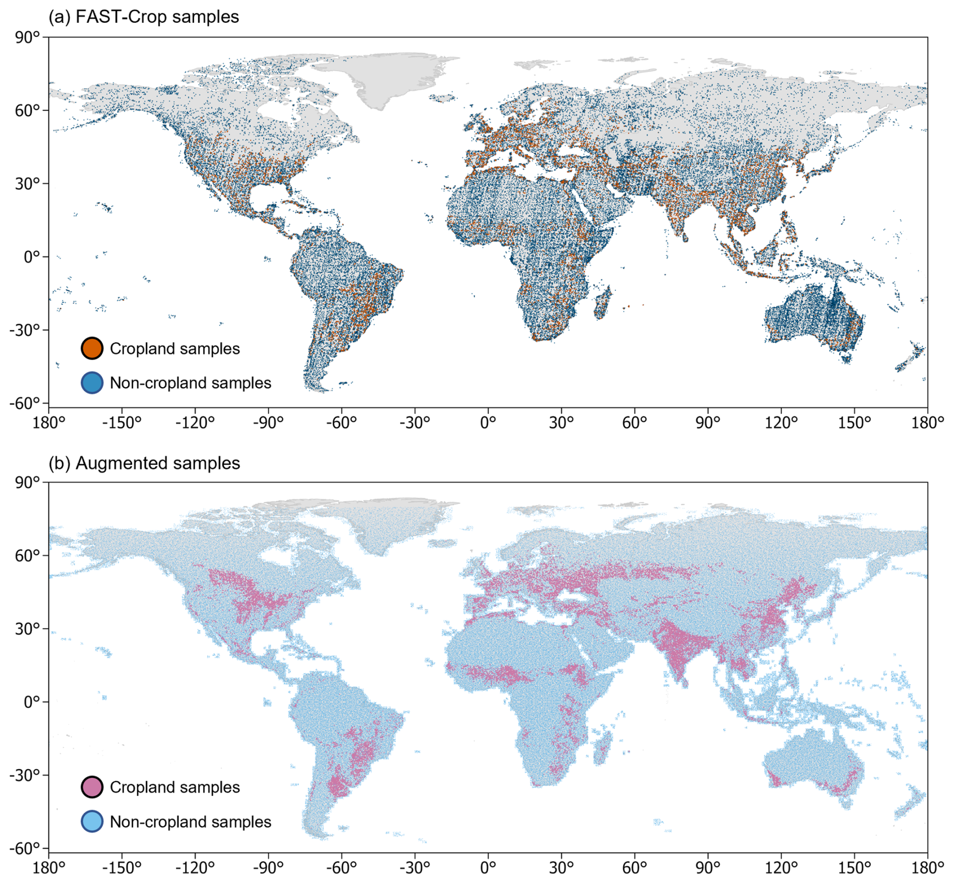
Figure 1 Spatial distribution of the training sample sets used for GACED30 generation. (a) FAST-Crop sample sets derived by expert annotation; (b) spatially augmented sample sets generated via rule-based expansion to improve global coverage.

To expand the geographical coverage of this expert-annotated baseline, we generated a spatially augmented sample set using global equal-area sampling and GLAD-based thematic stratification, followed by agreement screening with a FAST-Crop-trained classifier, spatial-spectral distribution screening, performance-guided subset selection, and year-specific weak-label screening (Sect. 3.2.1 and Sects. S1.1 and S1.2 in the Supplement). This multi-stage procedure yielded 332 471 retained sample locations. Because the augmented cropland tier predominantly represented categories included within the GLAD cropland definition, adding these samples reduced the combined proportion of Orchard and Greenhouse samples from approximately 11 % in the FAST-Crop cropland subset to approximately 3 % in the final cropland training set. The potential effect of this compositional shift was evaluated through the training-set ablation experiment reported in Sect. 4.1.1 and Sect. S1.3 in the Supplement.

2.3.2 Independent static validation samples

To provide an objective static thematic assessment of GACED30, we employed a validation set isolated entirely from model calibration. This subset was extracted from the temporally stable records of the FAST validation set (Li et al., 2017). The FAST project generated its validation data using a sampling protocol distinct from that used for the training data: whereas training sites were manually selected for spectral representativeness, validation samples were allocated through a probabilistic global equal-area random sampling design. This probability-based framework provided spatially distributed observations of global land-cover heterogeneity. Unlike the augmented training samples, these validation samples were not subject to GLAD-based stratification or automated agreement filtering, thereby preventing GLAD-conditioned candidate selection from being propagated into this assessment. The final validation set comprised 29 226 sample locations, including 3268 confirmed stable cropland samples. Because this subset emphasizes stable land-cover states, it assesses thematic agreement near the reference date rather than cropland gain, crop loss, or transition timing.

2.3.3 Independent multi-temporal transition reference samples

To complement the static FAST-Crop assessment, we used two external multi-temporal reference sources whose reference labels were not used in GACED30 training or spatiotemporal post-processing. The first was the global probability-based reference sample associated with GLAD Cropland, comprising 3500 sample locations with cropland interpretations for five four-year epochs: 2000–2003, 2004–2007, 2008–2011, 2012–2015, and 2016–2019 (Potapov et al., 2022). These observations supported the assessment of crop gain and crop loss between four pairs of adjacent epochs.

The second reference source was the European Union Land Use/Cover Area frame Survey (LUCAS), which provides harmonized in situ land-cover observations for the 2006, 2009, 2012, 2015, and 2018 survey campaigns (d'Andrimont et al., 2020), supplemented with observations from the 2022 campaign (d'Andrimont et al., 2024). Only locations with valid observations at both endpoints of a survey interval were retained.

GLAD Cropland provides global transition evidence across four adjacent four-year intervals, whereas LUCAS supplies denser repeated observations over five European survey intervals. Together, these datasets enable a targeted multi-temporal assessment of crop gain and crop loss, although their temporal spacing does not independently identify the exact year in which a transition occurred.

The GLAD Cropland reference samples are available at https://glad.umd.edu/dataset/croplands (last access: 22 September 2026). The LUCAS primary data are available from https://ec.europa.eu/eurostat/web/lucas/database/primary-data (last access: 22 September 2026).

2.4 National Agricultural Statistics (FAOSTAT)

To evaluate the agreement between our satellite-derived product and official national statistics, we compared the annual cropland area estimates from GACED30 with data from the Food and Agriculture Organization Corporate Statistical Database (FAOSTAT) (FAO, 2022). FAOSTAT compiles national land-use statistics reported by member countries through censuses and surveys. We obtained land-use statistics from the FAOSTAT Land Use domain (https://www.fao.org/faostat/en/#data/RL, last access: 22 September 2026) for 132 countries with observations available during 2000–2024.

2.5 Regional and agro-ecological reference datasets

For regional evaluation in China, we employed the China Annual Cropland Dataset (CACD), a 30 m annual cropland dataset covering 1986–2021 (Tu et al., 2024). CACD estimates annual cropland probabilities and applies LandTrendr trajectory segmentation together with a spatial–temporal consistency check to reduce interannual noise and refine its annual maps. These explicit temporal-refinement procedures make CACD a valuable regional benchmark for evaluating annual cropland time series. For the China-specific accuracy assessment, we used FAST-2015-China, the China subset of the FAST validation set in 2015 following the FROM-GLC classification system, to evaluate the 2015 GACED30 and CACD layers.

We additionally used the global 10 m reference dataset of Lesiv et al. (2025), hereafter GeoWiki2015. Its large collection of visually interpreted 10 m samples was used to derive a complementary estimate of temporary-crop area in China. We further used the Third National Land Survey (3rd NLS) as an official benchmark for 2019. The 3rd NLS reported 127.86 Mha of cultivated land and 20.17 Mha of garden land (State Council Third National Land Survey Leading Group Office et al., 2021). Their combined area of 148.03 Mha was compared with the full GACED30 Cropland estimate, whereas the cultivated-land area was compared with the GeoWiki2015 temporary-crop estimate.

To examine geographical variation in mapping performance, we used the Global Agro-Ecological Zones version 4 dataset (GAEZ v4; FAO and IIASA, 2021). The GAEZ thermal and moisture regimes were organized into 18 broad analytical strata spanning tropical, subtropical, temperate, and boreal environments under semi-arid, sub-humid, and humid moisture conditions. These strata were used to diagnose geographic variation in accuracy, not agricultural suitability.

3 Methods

The framework for generating the GACED30 dataset is illustrated in Fig. 2. This process integrates multi-source Earth observation data with machine learning to produce a harmonized 25-year annual record. The workflow comprises five main components: (1) feature engineering to construct a high-dimensional spectral-temporal space using SDC30; (2) annual cropland probability mapping using spectral-semantic sample alignment, year-specific weak-label screening, and year-specific CatBoost classification under a common mapping protocol; (3) spatiotemporal cropland extent refinement through a limited temporal rotation rule and morphological field reconstruction; (4) derivation of Structural Evolution Indicators, including cropping frequency and trend analysis; and (5) comprehensive global, regional, and agro-ecological evaluation using independent static samples, multi-temporal transition references, peer map products, agro-ecological strata, and agricultural statistics.

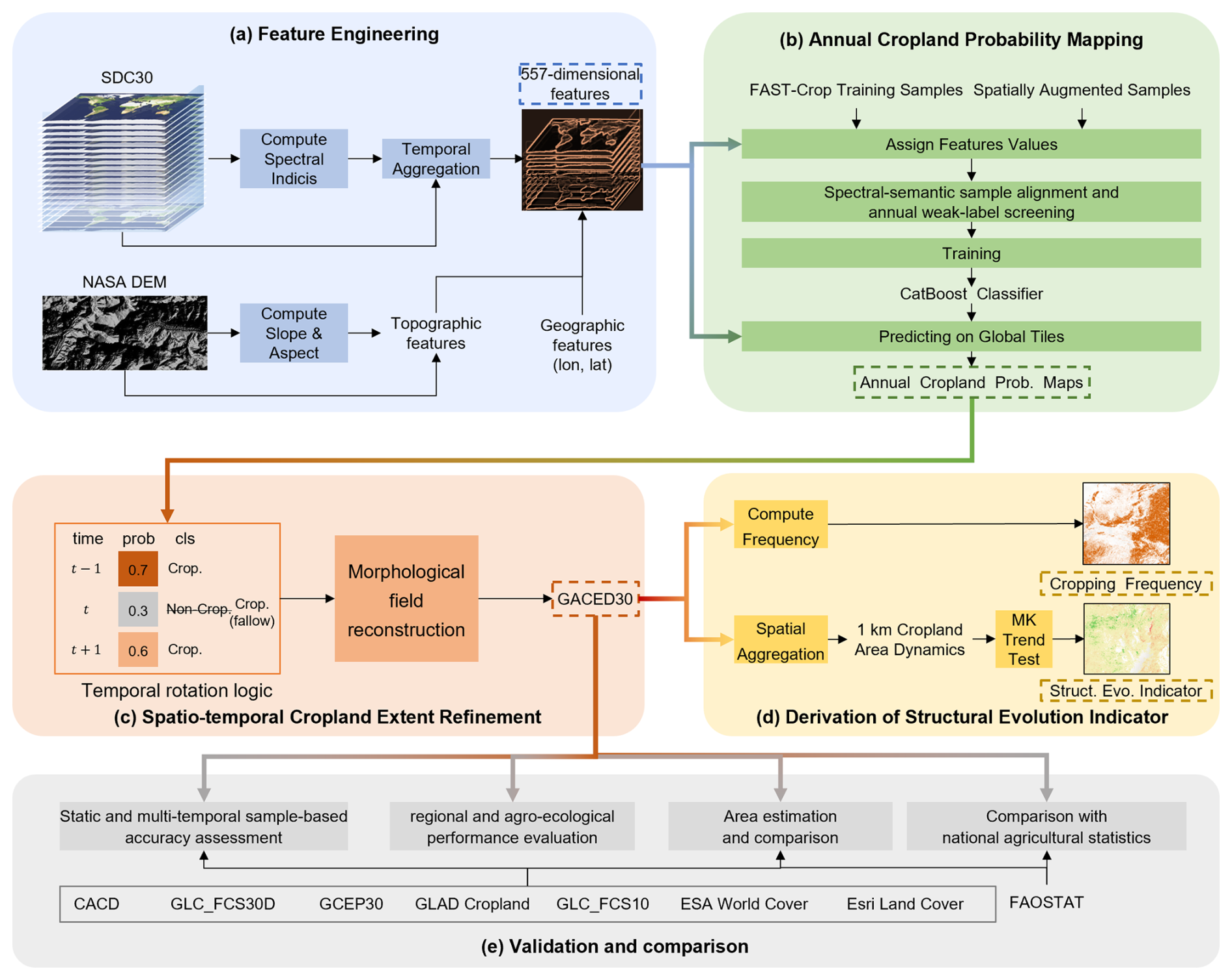
Figure 2 Workflow for generating and evaluating GACED30. (a) Feature engineering using SDC30 and NASADEM data. (b) Annual cropland probability mapping through multi-stage spectral-semantic sample alignment, annual weak-label screening, and year-specific CatBoost classification. (c) Spatiotemporal cropland extent refinement using temporal rotation logic and morphological field reconstruction. (d) Derivation of Structural Evolution Indicators, including cropping frequency and trend analysis. (e) Static thematic accuracy assessment, multi-temporal transition assessment, regional and agro-ecological performance evaluation, global and regional area estimation and inter-product comparison, and comparison with national agricultural statistics.

3.1 Feature engineering

Static spectral signatures alone are insufficient to distinguish active cropland from natural vegetation. Agricultural land is often characterized by phenological trajectories associated with sowing, biomass accumulation, and harvest. To capture this dynamic signal, we constructed a high-dimensional feature space based on the SDC30 time series (Fig. 2a).

While SDC30 offers daily resolution, global agricultural monitoring requires balancing temporal fidelity with computational feasibility. Therefore, we aggregated the daily reflectance into 8 d composites using a median reducer. This produced 46 evenly spaced observations per year, retaining phenological detail, including in double-cropping systems, while reducing residual noise. For each of the 46 time steps, we extracted 12 spectral components optimized for agricultural monitoring:

• Basic Spectral Bands (6): Blue, Green, Red, NIR, SWIR1, and SWIR2

• Biomass and Structure Indices (3): NDVI (general greenness), kNDVI (to minimize saturation in high-biomass crops) (Camps-Valls et al., 2021), and MNDWI (to capture paddy rice inundation).

• Tasseled Cap Components (3): Brightness, Greenness, and Wetness (to enhance soil and moisture detection).

This process generated a dense time-series vector of 552 features per pixel.

To further constrain the model against false positives in non-arable terrain, we appended five auxiliary features to the spectral vector. We utilized NASADEM to derive Elevation, Slope, and Aspect, helping the model distinguish flat arable land from natural vegetation on steep slopes, where extensive cultivation is generally less likely. Additionally, pixel-level Latitude and Longitude were included not merely as location variables, but to implicitly represent broad agro-climatic variation, allowing the model to adapt to geographical differences in crop calendars.

The final input vector comprised 557 features per pixel, combining the phenological depth of the time series with the physical constraints of the terrain.

3.2 Annual cropland probability mapping

To generate annual cropland probability maps under a common mapping framework, we first constructed spatially extensive and thematically harmonized annual training subsets through multi-stage sample alignment and year-specific weak-label screening (Sect. 3.2.1). We subsequently used year-specific CatBoost models to estimate pixel-wise cropland probabilities across the 2000–2024 archive (Sect. 3.2.2). The annual classifiers were trained independently, and direct temporal linkage between their outputs was introduced only through the limited post-classification rotation rule described in Sect. 3.3.1.

3.2.1 Spectral-semantic sample alignment and year-specific weak-label screening

To construct a spatially extensive and thematically harmonized training sample set, we implemented a four-stage sample-alignment strategy that combined the semantic detail of expert annotation with the broader geographical coverage provided by spatially stratified candidate sampling. We first generated approximately 360 000 candidate locations using a global equal-area sampling design stratified by GLAD Cropland (Potapov et al., 2022), with additional sampling directed toward underrepresented ecoregions. In Stage 1, a preliminary CatBoost classifier trained exclusively on the expert-annotated FAST-Crop samples was applied to these candidates. A candidate was retained only when its predicted Cropland/Non-cropland class agreed with the corresponding GLAD-stratified label. FAST-Crop therefore provided the semantic reference for agreement screening, whereas GLAD Cropland provided the initial spatial and thematic prior. Because GLAD Cropland and GACED30 differ in their treatment of permanent woody crops, agricultural structures, and active fallow, this screening reduced but did not eliminate definition-level conflicts.

In Stage 2, spatial, spectral, and category filtering was performed. The global land surface was divided into 5°×5° geographical grids. Within each grid, augmented candidates were sampled according to the statistical distribution of the six-band annual-median SDC30 surface-reflectance vector, drawing on the approximately Gaussian behaviour of log-transformed surface reflectance in homogeneous land-cover regions (Liao et al., 2026a). Category balancing was then performed by sampling the filtered augmented candidates according to the Cropland/Non-cropland proportions of FAST-Crop within each grid. In Stage 3, the remaining candidates were optimized using the sample-size–performance scaling relationship established by Liao et al. (2026b). At each iteration, alternative 10 000-sample batches were evaluated, and the batch producing the highest estimated asymptotic performance was retained. Iterations were stopped once the retained augmented-sample total reached the target of approximately 340 000. Detailed implementation settings are provided in Sect. S1.1 and Table S1 in the Supplement.

The augmented samples nevertheless remained conditioned on the GLAD spatial prior. In particular, the combined proportion of Orchard and Greenhouse samples decreased from approximately 11 % in the FAST-Crop cropland subset to approximately 3 % in the final cropland training sample set. We therefore evaluated the sensitivity of individual FAST-Crop subclasses to the addition of the GLAD-conditioned augmented samples through the controlled training-set comparison reported in Sect. 4.1.1 and Sect. S1.3.

Finally, annual weak labels were assigned directly to the selected spatial samples for 2000–2024. For 2000–2019, the label from each GLAD Cropland epoch was assigned to every year covered by that epoch; because GLAD Cropland provides no subsequent epoch, the 2016–2019 labels were also used as the initial weak labels for 2020–2024. For each year, five-fold out-of-fold CatBoost probabilities were generated using StratifiedKFold(n_splits=5, shuffle=False) and supplied to CleanLab's default find_label_issues procedure (Northcutt et al., 2021). FAST-Crop labels were treated as fixed reference labels and were excluded from possible pruning, whereas only the augmented point-year labels were eligible for screening. No manually selected probability or confidence threshold was applied. An augmented point-year flagged by CleanLab was excluded from the training sample set for the corresponding annual classifier, and an augmented location was removed entirely when more than 25 % of its 25 annual labels were flagged, corresponding to at least seven years. This procedure screens year-specific weak-label conflicts rather than imposing a transition rule between adjacent years. The annual training subsets therefore shared the same expert-reference basis, feature definition, sample-construction framework, and screening procedure, but were not identical because augmented point-year labels could be excluded separately for each annual classifier. After annual weak-label assignment and screening, the final augmented sample set contained 332 471 locations, comprising approximately 25 000 Cropland and 307 000 Non-cropland samples.

3.2.2 Annual probability estimation

Following construction of the annual training subsets, we trained independent year-specific classifiers to account for interannual phenological variability. For each year from 2000 to 2024, the corresponding valid FAST-Crop and augmented samples were used to train a CatBoost classifier (Prokhorenkova et al., 2018). The preliminary screening classifier, the models used to generate out-of-fold probabilities for CleanLab, and the final annual classifiers shared the same core CatBoost configuration, which is reported in Sect. S1.1 and Table S1.

CatBoost was selected because its ordered-boosting mechanism mitigates prediction shift in conventional gradient-boosted decision trees, while its oblivious-tree structure efficiently handles the 557-dimensional spectro-temporal feature space without manual feature reduction. To assess this choice empirically, we compared CatBoost with Random Forest and XGBoost using the same training-sample and feature framework. Predictive performance was measured using F₁ score, and computational efficiency was represented by observed full-batch inference throughput (Sect. S1.2 and Table S2 in the Supplement).

The trained year-specific CatBoost models were applied to the corresponding annual SDC30 feature stacks to generate pixel-wise cropland probability maps for 2000–2024. Because these classifiers were fitted independently, no parameter sharing, temporal regularization, or explicit model-level coupling was imposed between adjacent years. Cross-year comparability instead relies on the harmonized SDC30 inputs and the common feature, sample-construction, and model protocols. These elements standardize annual mapping, while temporal linkage is limited to the postclassification rotation rule in Sect. 3.3.1. Production training and inference were performed on the high-performance iEarth remote-sensing cloud computing platform hosted by Pengcheng Laboratory.

3.3 Spatiotemporal cropland extent refinement

The raw probability maps generated in the previous step capture annual phenological signals but inevitably contain salt-and-pepper noise and temporal flickering caused by residual observational uncertainty or phenological ambiguity. A particular challenge lies in the spectral confusion between active fallow and natural bareland: both exhibit low vegetation indices, yet active fallow represents a functional phase of a cropping cycle and is therefore included as Cropland. To transform these pixel-level probabilities into a spatially coherent cropland dataset, we applied a spatiotemporal refinement framework designed to improve field-level spatial structure and correct a restricted class of locally implausible one-year sequences (Fig. 2c).

3.3.1 Limited temporal rotation rule

Because the annual CatBoost models were trained independently, temporal evidence was introduced after classification through a limited rotation rule targeting uncertain observations. Specifically, we identified pixels within the probability interval ($P\in [\mathrm{0.3},\mathrm{0.5}]$), which would otherwise be classified as Non-cropland under the standard binary threshold.

For a pixel in year t, an uncertain observation within this interval was retained as Cropland under a temporary-fallow interpretation only when the same pixel was classified as Cropland (P>0.5) in both the preceding (t−1) and following (t+1) years. This rule bridges isolated one-year gaps that are compatible with temporary fallow or weak phenological signals. The temporal context reduces, but does not eliminate, confusion with spectrally similar pasture, rangeland, or bare surfaces. The rule does not alter observations with probabilities below 0.3, smooth complete pixel trajectories, or impose general temporal consistency across the annual series.

3.3.2 Morphological field reconstruction

Following temporal refinement, the probability maps were binarized to generate initial boolean masks. We then applied morphological filtering to improve spatial coherence. Large contiguous fields are common in intensive agricultural regions, whereas isolated pixels and narrow fragments often reflect classification noise. Raw pixel-based classification, however, often results in “salt-and-pepper” noise that misrepresents field boundaries. To address this, we designed a morphological filter to identify and remove spurious cropland detections that violate shape regularity. We specifically targeted and removed artifacts defined by weak connectivity or insufficient area, including:

• Isolated single pixels lacking immediate neighbours

• Small linear fragments (e.g., 1 pixel×2 pixel strips) that do not form a cohesive field structure

• Diagonally connected clusters (checkerboard patterns) that lack 4-connectivity

By removing these fragmented clusters, the filter reduced pixel-scale artifacts and improved the spatial coherence of the mapped cropland parcels.

3.4 Derivation of Structural Evolution Indicators

To characterize the spatiotemporal dynamics of global agricultural systems from 2000 to 2024, we developed a grid-based analytical framework combining mapped cropland persistence with directional trend analysis (Fig. 2d).

First, we calculated pixel-level Cropping Frequency (F_crop), defined as the proportion of the 25 annual layers in which a pixel was classified as Cropland. This metric summarizes the temporal persistence of mapped cropland status, distinguishing persistently mapped cropland from pixels with low or intermediate frequencies. Cropping Frequency alone does not determine the direction of change: for example, the same frequency could result from recent cropland expansion or from cropland present only during the earlier part of the record.

To resolve this ambiguity and identify the directional evolution of these landscapes, we derived Structural Evolution Indicators from GACED30 using a grid-based trend analysis framework (Fig. 2d). Area calculations were performed in a global equal-area projection following the practical principles outlined by Tyukavina et al. (2025). The annual 30 m binary cropland maps were aggregated to 1 km×1 km grid cells, and mapped cropland area was summed within each grid cell for each year. This produced a 25-observation annual cropland-area series for each analysed grid cell over 2000–2024. The non-parametric Mann–Kendall (MK) test and Theil–Sen estimator were applied to each time series, yielding the MK significance level (p), the Theil–Sen slope (β, ha yr⁻¹), and the confidence interval of the slope. Using the minimum slope threshold τ, grid cells with β>τ, $\mathit{\beta }<-\mathit{\tau }$, and $\left|\mathit{\beta }\right|\le \mathit{\tau }$ were classified as general expansion, general reduction, and stable, respectively. Expansion and reduction were additionally classified as stringent when the corresponding Mann–Kendall test satisfied p<0.01.

The minimum slope threshold τ is an operational choice that depends on the spatial aggregation unit, study duration, and analytical objective. For the principal analysis in this study, we adopted τ=0.2 ha yr⁻¹ as an operational grid-scale threshold. Because a 1 km×1 km grid cell covers approximately 100 ha, this value corresponds to a linear trend equivalent to 0.2 % of the grid area per year and to 4.8 ha, or 4.8 % of the grid area, across the 24 elapsed annual intervals between 2000 and 2024. It therefore provides an interpretable minimum magnitude for identifying landscape-scale structural change over the study period.

Although 0.2 ha corresponds to approximately 2.2 nominal 30 m pixels, τ applies to the slope estimated from the complete 25-year cropland-area trajectory, not to a single-year pixel-count change. Instead, β is estimated from the complete 25-year cropland-area trajectory within each grid cell. We therefore evaluated the sensitivity of both classifications using τ values from 0.10 to 0.50 ha yr⁻¹ at intervals of 0.05 ha yr⁻¹ (Figs. S1 and S2 in the Supplement).

Compared with bi-temporal differences between multi-year epochs, analysis of all 25 annual observations reduces sensitivity to the selection of baseline and endpoint windows and limits the influence of short-lived fluctuations. The Mann–Kendall test and Theil–Sen estimator quantify the statistical support, direction, and magnitude of mapped trends under the specified criteria. These statistics do not independently establish the cause of a trend or guarantee that every mapped change represents a permanent land-cover conversion.

3.5 Validation and comparison

To assess the quality and reliability of GACED30, we adopted five complementary approaches (Fig. 2e): (1) static thematic accuracy assessment using the independent FAST-Crop validation samples; (2) multi-temporal assessment of crop gain and crop loss using GLAD Cropland and LUCAS reference samples; (3) matched regional evaluation in China together with agro-ecological-zone-stratified accuracy assessment; (4) global and regional area estimation and inter-comparison with existing global and regional cropland products; and (5) comparison with national agricultural statistics from FAOSTAT. These components respectively evaluate static thematic agreement, transition detection across multiple intervals, regional and environmental variations in performance, sample-adjusted area trajectories, and aggregated national-scale consistency.

3.5.1 Static thematic accuracy assessment

We evaluated the pixel-level accuracy of GACED30 using the independent FAST-Crop validation set. For each validation sample observed in year T_sample, we selected the closest available layer from GACED30 or each peer product by minimizing $|T_{\text{sample}}-T_{\text{product}}|$.

We calculated a binary confusion matrix (Cropland vs. Non-cropland) to derive standard quantitative accuracy metrics. Let n_ij denote the number of samples classified as class i in the map but belonging to class j in the reference data, where k=2 is the number of classes, and N is the total number of samples. The specific metrics are calculated as follows.

Overall Accuracy (OA) represents the proportion of correctly classified pixels:

$$\begin{array}{}\text{(1)}& \text{OA}={\displaystyle \frac{{\sum }_{i=\mathrm{1}}^k{n}_{ii}}{N}}\end{array}$$

Producer's Accuracy (PA), which relates to omission error, indicates the probability that a ground reference pixel is correctly classified in the map:

$$\begin{array}{}\text{(2)}& {\text{PA}}_i={\displaystyle \frac{n_{ii}}{n_{+i}}}\end{array}$$

where n_+i is the total number of reference samples for class i.

User's Accuracy (UA), which relates to commission error, indicates the probability that a pixel classified as class i on the map actually represents that class on the ground:

$$\begin{array}{}\text{(3)}& {\text{UA}}_i={\displaystyle \frac{n_{ii}}{n_{i+}}}\end{array}$$

where n_i+ is the total number of map predictions for class i.

The F₁ score is the harmonic mean of the precision and recall. It thus symmetrically represents both precision and recall in one metric.

$$\begin{array}{}\text{(4)}& {\mathrm{F}}_{\mathrm{1}}\text{score}={\displaystyle \frac{\mathrm{2}\times \text{UA}\times \text{PA}}{\text{UA}+\text{PA}}}\end{array}$$

The Kappa Coefficient (κ) measures the agreement between the classification map and reference data while accounting for chance agreement:

$$\begin{array}{}\text{(5)}& \mathit{\kappa }={\displaystyle \frac{P_{\mathrm{o}}-P_{\mathrm{e}}}{\mathrm{1}-P_{\mathrm{e}}}}\end{array}$$

where P_o is the observed agreement (OA), and P_e is the hypothetical probability of chance agreement, calculated as:

$$\begin{array}{}\text{(6)}& P_{\mathrm{e}}={\displaystyle \frac{{\sum }_{i=\mathrm{1}}^k(n_{i+}\times n_{+i})}{N^{\mathrm{2}}}}\end{array}$$

To benchmark the performance of GACED30, we applied these metrics to conduct a comparative accuracy assessment against the GLAD Cropland product (Potapov et al., 2022), as well as other available global land cover datasets including 30 m products (GCEP30, Thenkabail et al., 2021, GLC_FCS30D, Zhang et al., 2024b) and 10 m products (GLC_FCS10, Zhang et al., 2025c, ESA WorldCover, Zanaga et al., 2022, Esri Land Cover, Karra et al., 2021). All products were evaluated against the same FAST-Crop reference labels following the cropland definition described in Sect. 2.1. Because the native product legends differ in their treatment of orchards and other perennial woody crops, active fallow, and temporary meadows and pastures, part of the observed disagreement may reflect definitional differences. Additionally, since the FAST-Crop validation subset predominantly represents stable land-cover states, these metrics evaluate static thematic agreement and are not interpreted as direct validation of cropland transitions.

3.5.2 Multi-temporal transition assessment

We evaluated two directional transitions separately: Cropland to Non-cropland, hereafter termed crop loss, and Non-cropland to Cropland, hereafter termed crop gain. For each directional assessment, the target transition was treated as the positive class, whereas stable pairs and the opposite transition were treated as negative cases. These sample-level transitions provide a targeted assessment of change detection but are not identical to the 1 km structural expansion and reduction classes, which are derived from trends fitted to the complete 25-year annual record.

For the GLAD Cropland assessment, the annual binary layers of GACED30 and GLC_FCS30D were aggregated within each corresponding four-year epoch using the pixel-wise median. Crop gain and crop loss were then determined for each of the four adjacent-epoch intervals: 2000–2003 to 2004–2007, 2004–2007 to 2008–2011, 2008–2011 to 2012–2015, and 2012–2015 to 2016–2019. The mapped transitions were evaluated against the corresponding GLAD reference transitions at the same sample locations. Each valid location–interval pair was treated as one observation, and the four intervals were pooled for the overall assessment. The same temporal aggregation, spatial extraction, and class-harmonization procedures were applied to GACED30 and GLC_FCS30D.

For LUCAS, valid observations at the same location in successive available surveys were paired. The corresponding annual GACED30 and GLC_FCS30D classes were extracted for the two survey years, and the reference and mapped transitions were determined from their respective endpoint classes. When a location occurred in more than one survey interval, each location–interval pair was treated as one unweighted observation. Results from the 2006–2009, 2009–2012, 2012–2015, 2015–2018, and 2018–2022 intervals were pooled for the overall assessment.

Class harmonization was performed before determining the transitions. GACED30 class 10 was treated as Cropland. For LUCAS, land-cover codes B, B11–B19, B21–B23, B31–B37, B41–B45, B51–B54, B71–B77, B81–B84, BX1, and BX2 were mapped to Cropland. Temporary grassland (B55) was mapped to Grassland and was therefore excluded. For GLC_FCS30D, classes 10, 11, 12, and 20 were mapped to Cropland, whereas class 130 was treated as Grassland. Consequently, permanent crops were included, temporary grasslands were excluded, and fallow land was not automatically assigned to Cropland but followed its original observed or product land-cover class.

Because stable observations predominated in both reference sources, overall accuracy was not used as the principal transition metric, as it would be dominated by unchanged pairs. The resulting metrics were interpreted within the spatial, temporal, and semantic support of each reference dataset.

3.5.3 Regional and agro-ecological evaluation

We evaluated the 2015 GACED30 and CACD layers using the FAST-2015-China validation sample set. OA and cropland-specific UA, PA, and F₁ were calculated from the confusion matrix following the definitions provided in Sect. 3.5.1.

For the national area assessment, we compared the China-specific GACED30 estimates produced using the FAST-Crop area-adjustment estimator described in Sect. 3.5.4 with two complementary regional benchmarks. The adjusted GACED30 estimate for 2019 and its 95 % confidence interval were compared with the combined cultivated-land and garden-land area reported by the 3rd NLS. For 2021, we compared the adjusted GACED30 estimate with the published sample-adjusted CACD estimate and its reported 95 % confidence interval (Tu et al., 2024). Given differences in classification scope, observation protocol, spatial representation, and area estimation, these comparisons were interpreted as consistency checks.

Finally, each independent FAST-Crop static validation record was spatially assigned to one of the 18 agro-ecological strata derived from GAEZ v4. OA, UA, PA, F₁ score, and Kappa were then calculated separately for each stratum. Where a stratum contained no positive Cropland reference cases, cropland-specific UA, PA, F₁, and Kappa were considered not applicable and reported as NA rather than as zero accuracy.

3.5.4 Global and regional area estimation and inter-comparison

To ensure accurate area estimation within a consistent and reproducible framework, we utilized Open Data Cube (ODC) technology to manage and process all multi-source datasets (Killough, 2018; Killough et al., 2020). Rather than reprojecting all data into a single global system – which can introduce resampling artifacts – we maintained the native projections of each product and calculated areas using projection-specific protocols derived from Tyukavina et al. (2025).

For datasets provided in UTM projections (including GACED30 and Esri Land Cover), we calculated the area separately for each UTM zone to minimize geometric distortion, summing the results to derive global totals as per the zonal guidelines in Tyukavina et al. (2025). For datasets provided in EPSG:4326 (Geographic Lat/Lon) (including ESA WorldCover, GLAD Cropland, GLC_FCS30D, and the geographic version of Esri Land Cover), we retained the native grid and calculated pixel areas using the latitude-weighted geodetic formula described by Tyukavina et al. (2025), which accounts for the convergence of meridians towards the poles.

To ensure a consistent inter-product comparison, we applied the same sample-based area-adjustment framework to all map products shown in Fig. 6a. The FAST-Crop reference set was generated using stratified random sampling based on the underlying land-surface classes, together with a global equal-area hexagonal framework for spatial stratification. For each product, one product-specific binary confusion matrix was constructed using the available layer or epoch closest to the FAST-Crop reference imagery time. For every available year or epoch, the CRS-aware mapped Cropland and Non-cropland area proportions were combined with the corresponding product-specific confusion matrix to obtain sample-adjusted global cropland areas. Standard errors and 95 % confidence intervals were calculated consistently following Olofsson et al. (2014) and Tyukavina et al. (2025). This procedure retains the product-specific omission and commission patterns while placing all area estimates relative to the same FAST-Crop reference definition. Applying a fixed confusion matrix across each product series assumes that its error structure remains reasonably stable over the corresponding temporal coverage.

For the China-specific area assessment, the same adjustment procedure was applied separately using the FAST-2015-China and GeoWiki2015 reference samples. The mapped Cropland and Non-cropland areas were combined with the corresponding confusion matrices to derive sample-adjusted estimates for 2019. The FAST-Crop-based estimate represents the full GACED30 Cropland definition, whereas the GeoWiki2015-based estimate primarily represents temporary crops. The standard error and 95 % confidence interval of the FAST-Crop-based estimate were calculated following Olofsson et al. (2014). To avoid repeatedly using observations from the same validation sites across years, the area adjustment was updated using only the FAST-2015-China.

3.5.5 Comparison with national agricultural statistics

National statistics provide a crucial independent benchmark for evaluating the reliability of satellite-derived area estimates. We compared the aggregated national cropland areas from GACED30 with official statistics from FAOSTAT.

To facilitate a rigorous comparison, we reconciled the FAOSTAT aggregates to match the definition of GACED30 (Sect. 2.1). The standard FAO definition of “Cropland” (Item 6620) comprises “Arable land” (Item 6621) and “Permanent crops” (Item 6650). However, the sub-category “Arable land” includes “Temporary meadows and pastures” (Item 6633) – defined as land cultivated with herbaceous forage for less than five years. Because GACED30 excludes “Temporary meadows and pastures” (Item 6633), we subtracted this category from total FAO “Cropland” (Item 6620), following Tubiello et al. (2023b). This adjusted metric, encompassing annual temporary crops, temporary fallow, and permanent woody crops (orchards), aligns with our mapped classes and serves as the benchmark for assessing national-scale area agreement and long-term trends of the GACED30 dataset. We utilized the Coefficient of Determination (R²) and Normalized Root Mean Square Error (NRMSE) to quantify the correlation between the GACED30-derived areas and the adjusted FAOSTAT statistics across all available countries.

Beyond static area comparisons, we further evaluated the consistency of long-term cropland dynamics by benchmarking the net area change derived from GACED30 against FAOSTAT trends. We calculated the net area change for each country over the study period (2000–2024). To mitigate the impact of inter-annual fluctuations (e.g., extreme weather events) and reporting inconsistencies, we adopted a robust multi-year averaging approach, defining net change as the difference between the mean area of the last three available years and the mean area of the first three available years. We restricted this analysis to countries with records spanning at least 10 years and with a material change reported by FAOSTAT, defined as an absolute net change exceeding either 0.5 % of the reference cropland area or 1000 ha. This filtering focuses the comparison on substantial long-term changes rather than minor reporting fluctuations. The agreement was quantified using two metrics: the Direction Match Rate, which measures the percentage of countries where GACED30 and FAOSTAT report the same trajectory (expansion or contraction), and the Weighted Match Rate, which weights this agreement by the total cropland area of each country to emphasize performance in major agricultural nations.

4 Results

4.1 Quantitative evaluation

4.1.1 Static thematic accuracy assessment

To assess static thematic agreement, we evaluated GACED30 using the independent FAST-Crop stable-site validation set, which was excluded from model training. We then compared GACED30 with six global 10 and 30 m land-cover or cropland products: GLAD Cropland, GCEP30, GLC_FCS30D, GLC_FCS10, ESA WorldCover, and Esri Land Cover.

As shown in Table 2, GACED30 achieved the highest OA (0.965), F₁ score (0.844), UA (0.883), and PA (0.808) among the evaluated products. Its F₁ score exceeded those of GLAD Cropland and ESA WorldCover by 0.100 and 0.122, respectively. These results demonstrate strong static thematic agreement between GACED30 and the independent FAST-Crop validation samples under the adopted Cropland/Non-cropland definition.

Table 2 Static thematic accuracy of GACED30 and peer products against the independent FAST-Crop stable-site validation set.

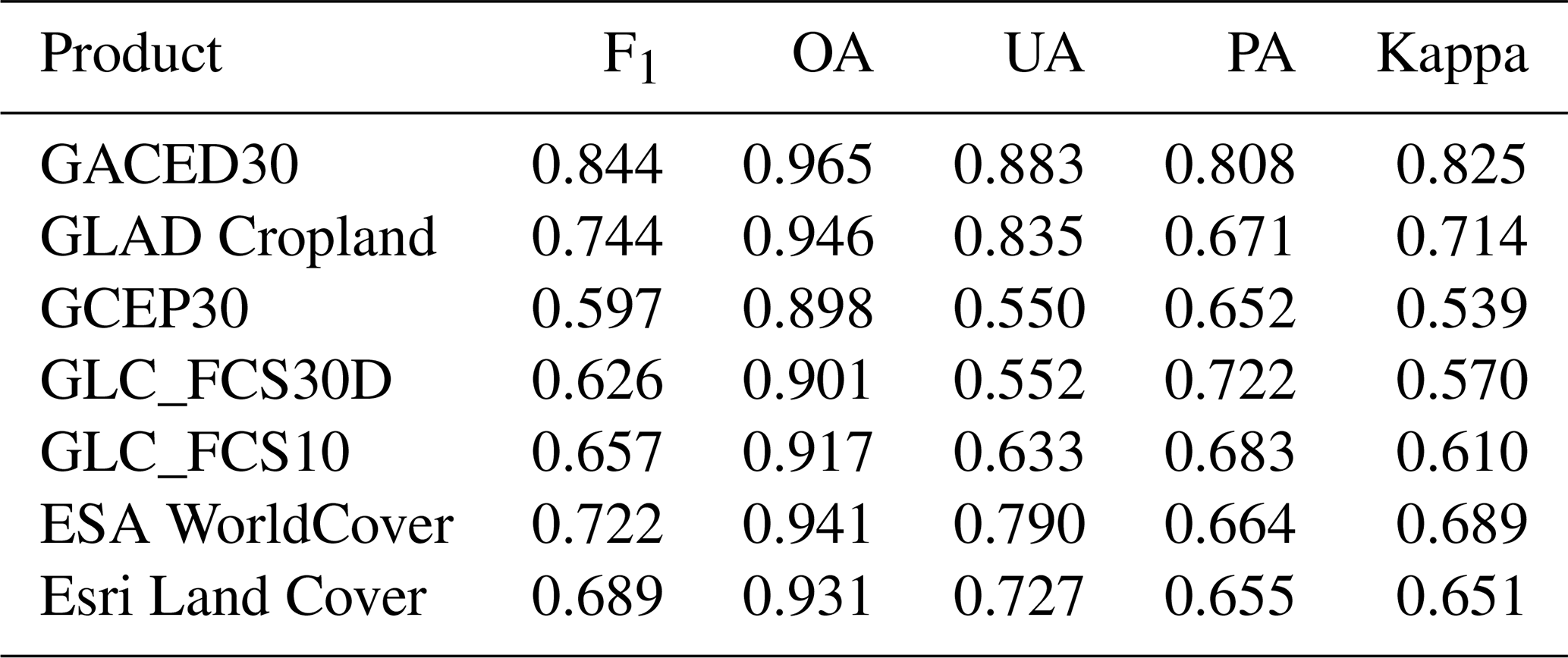
Part of the mismatch with peer products may reflect differences in cropland definitions rather than mapping errors alone. Specifically, GACED30 includes orchards and active fallow but excludes temporary meadows and pastures, whereas peer products differ in their treatment of these categories. Temporal mismatches between the validation samples and product layers may also contribute to the observed differences. Table 2 therefore compares relative agreement with the adopted FAST-Crop/GACED30 definition; transition performance is evaluated separately in Sect. 4.1.2.

The classifier benchmark provided additional empirical support for selecting CatBoost (Table S2). CatBoost achieved the highest F₁ score of 0.8358, compared with 0.832 for XGBoost and 0.828 for Random Forest. On the common NVIDIA A100 platform, CatBoost processed 3 148 493 samples s⁻¹, compared with 719 361 samples s⁻¹ for XGBoost, corresponding to approximately 4.4 times the observed full-batch GPU inference throughput. Random Forest processed 163 614 samples s⁻¹ on the CPU platform. Because Random Forest and the two boosting models were evaluated on different processor architectures, the Random Forest throughput is reported as an implementation-specific reference rather than a hardware-normalized comparison. Overall, CatBoost provided the highest observed F₁ score and the fastest GPU inference among the evaluated implementations.

We further conducted a training-set ablation experiment to examine whether adding the GLAD-conditioned augmented samples affected binary cropland recognition for the second-level FAST-Crop subclasses (Table S3 in the Supplement). Adding the augmented samples increased F1 by 0.025 for Other Farmland, 0.035 for Bare Farmland, and 0.055 for Greenhouse. Orchard showed a smaller decrease of 0.017, from 0.574 to 0.557, whereas Rice Paddy decreased by 0.055. Thus, despite the reduction in the relative representation of Orchard and Greenhouse samples, the FAST-Crop tier continued to support orchard recognition, with only a small observed decrease in Orchard performance. Nevertheless, the analysis qualifies rather than eliminates the potential influence of GLAD-conditioned augmentation on categories outside the GLAD cropland definition. Because each subclass was evaluated separately against non-cropland, these results should be interpreted as a binary sensitivity analysis rather than a multiclass subclass assessment.

4.1.2 Multi-temporal transition assessment

The multi-temporal assessment (Table 3) provides a targeted evaluation of crop gain and crop loss that is not available from the stable-site FAST-Crop samples. Across the four pooled adjacent GLAD Cropland epoch intervals, GACED30 achieved higher recall and F₁ score than GLC_FCS30D for both transition directions. For crop loss, its recall and F₁ score were 0.177 and 0.178, compared with 0.129 and 0.152 for GLC_FCS30D. For crop gain, the corresponding values were 0.199 and 0.212 for GACED30 and 0.171 and 0.197 for GLC_FCS30D. GACED30 nevertheless had slightly lower precision: 0.180 versus 0.186 for crop loss and 0.227 versus 0.232 for crop gain.

The pooled LUCAS comparison showed larger differences between the products. For crop loss, GACED30 achieved precision, recall, and F₁ score values of 0.099, 0.072, and 0.083, respectively, compared with 0.062, 0.016, and 0.026 for GLC_FCS30D. For crop gain, GACED30 obtained values of 0.113, 0.058, and 0.076, whereas GLC_FCS30D obtained 0.057, 0.014, and 0.023.

Table 3 Pooled transition detection by GACED30 and GLC_FCS30D using the GLAD Cropland and LUCAS multi-temporal reference samples.

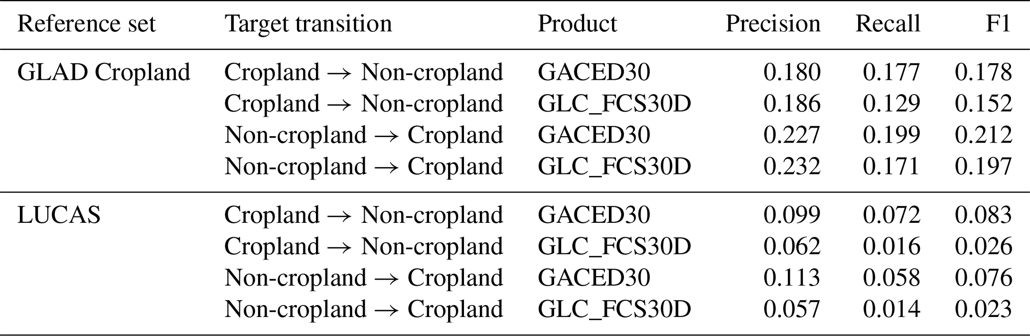
Note: GLAD Cropland results pool four transitions between adjacent four-year epochs spanning 2000–2019 after pixel-wise median aggregation of the annual product layers within each epoch. LUCAS results pool five successive survey intervals between 2006 and 2022. Each valid location–interval pair was treated as one observation, and metrics are reported as proportions.

Across both reference assessments, GACED30 showed higher transition recall and F₁ scores, although the absolute values remained modest and GLAD-based precision was slightly lower than for GLC_FCS30D. Transition detection requires correct classification at both temporal endpoints, so an error at either endpoint can generate an incorrect change label. The low prevalence of transitions, temporal aggregation, spatial-support differences, and residual semantic differences further affect these metrics. The common-sample comparison assesses transitions across multiple intervals under harmonized definitions but not their exact annual timing.

4.1.3 Regional and agro-ecological performance

The FAST-2015-China assessment showed that GACED30 achieved an OA of 0.946 and cropland-specific UA, PA, and F1 of 0.838, 0.843, and 0.840, respectively, compared with 0.940, 0.830, 0.810, and 0.820 for CACD. The two products therefore showed comparable overall performance, with GACED30 achieving slightly higher cropland-specific accuracy. GACED30 mainly benefits from harmonized, gap-free SDC30 observations and the strong classification capacity of CatBoost. CACD has a particular methodological advantage in spatiotemporal consistency. By combining annual cropland probabilities with LandTrendr trajectory segmentation, transition rules, and spatiotemporal consistency checking, CACD integrates information across years and neighboring pixels to reduce isolated classification errors and implausible temporal fluctuations. This design produces more coherent annual sequences, especially in heterogeneous agricultural landscapes and areas experiencing complex cropland changes.

The raw mapped cropland area of GACED30 in China in 2019 was 168.07 Mha. Adjustment using the 2015 FAST-Crop samples increased this estimate to 179.70 Mha, with a standard error of 3.98 Mha and a 95 % confidence interval of 171.91–187.50 Mha. The adjustment added 30.86 Mha of estimated omitted cropland from the mapped Non-cropland area and removed 19.23 Mha of estimated commission error, producing a net increase of 11.63 Mha. The adjusted estimate was 31.67 Mha, or 21.4 %, higher than the combined cultivated-land and garden-land area of 148.03 Mha reported by the 3rd NLS. In contrast, the GeoWiki2015 adjustment produced a temporary-crop estimate of 149.44 Mha, which remained 21.58 Mha, or 16.9 %, higher than the 3rd NLS cultivated-land area of 127.86 Mha.

The consistently higher values from the raw map and the two reference-sample adjustments show that the positive area difference is not specific to one reference dataset. The broader GACED30 definition contributes to this difference, particularly relative to the cultivated-land category alone, but does not fully explain it because the GeoWiki2015 temporary-crop estimate is also higher. Additional differences may arise because GACED30 represents cropland as 30 m raster pixels, whereas the 3rd NLS delineates land-use parcels using higher-resolution imagery and field investigation; mixed pixels along field boundaries can therefore affect the resulting totals. In 2021, the corresponding GACED30 estimate was approximately 180.00 Mha, remaining within the 95 % confidence interval of the published CACD estimate of 172.52 ± 21.24 Mha.

The AEZ-stratified results further showed that global accuracy was not spatially uniform (Table S4 in the Supplement). Across the tropical, subtropical, and temperate strata represented by AEZs 1–15, OA ranged from 0.931 to 0.997 and F₁ ranged from 0.631 to 0.913. The warm, humid subtropical stratum achieved the highest F₁ score among these zones (0.913), with a UA of 0.905 and a PA of 0.922. The lowest F₁ score occurred in the cool, humid tropical stratum (0.631), where the relatively high UA of 0.861 was accompanied by a substantially lower PA of 0.498. This contrast indicates that omission of cropland was the principal source of error in this environment and that its high OA of 0.951 partly reflected the predominance of Non-cropland reference records. The boreal sub-humid and humid strata contained no positive Cropland reference cases and therefore did not support the calculation of cropland-specific accuracy metrics.

4.1.4 Statistical consistency with FAO national statistics

To evaluate national-scale area consistency, we aggregated the GACED30 classifications into national totals and compared them with definition-reconciled FAOSTAT statistics. Across 132 countries, GACED30 achieved an R² of 0.95 and an NRMSE of 3.7 % (Fig. 3a). These metrics indicate close agreement in country-level cropland area after definition reconciliation but do not measure pixel-level thematic accuracy or transition detection.

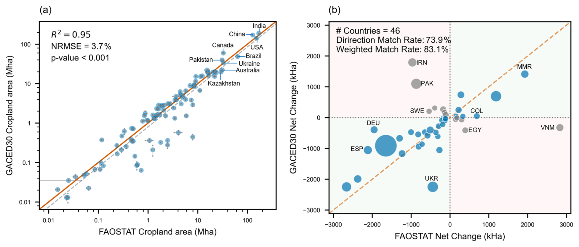
Figure 3 Consistency between GACED30 and FAOSTAT national statistics. (a) Comparison of mean annual cropland area (Mha) for 132 countries. The solid orange line indicates the 1:1 relationship; error bars represent the inter-annual standard deviation. (b) Comparison of long-term net area change (kHa) from 2000 to 2024 for 46 countries with significant reported dynamics. Bubbles are scaled by total cropland area, with blue indicating directional agreement and grey indicating disagreement.

For broader context, these values can be compared with those reported for other global cropland products in Table D1 of Tubiello et al. (2023a). Because those values were obtained using different product years, cropland definitions, and comparison protocols, they provide contextual information on the magnitude of national-area agreement rather than a controlled inter-product ranking. The sample-based assessments in Sects. 4.1.1–4.1.3 provide the more direct comparisons of static thematic, multi-temporal transition, and regional performance.

Beyond national area levels, we compared the long-term net change derived from GACED30 with FAOSTAT for 46 countries reporting substantial cropland dynamics (Fig. 3b). The directional match rate was 73.9 %, and the area-weighted match rate was 83.1 %. These results support agreement in the aggregated direction of long-term cropland change, particularly for major agricultural countries. Because the comparison is based on national totals, it does not validate the spatial location of changes, their exact annual timing, or their underlying causes.

Remaining discrepancies can arise from several sources, including mixed pixels at 30 m, fragmented agricultural parcels, differences between mapped land cover and administratively reported land use, residual definitional differences, and errors in either data source. In smallholder and highly fragmented landscapes, cultivated parcels may occupy only part of a Landsat pixel, causing their spectral signal to be mixed with surrounding non-cropland (Pax-Lenney and Woodcock, 1997).

For China, GACED30 estimates were also higher than the corresponding FAOSTAT values. As further demonstrated through the comparisons with CACD and the 3rd NLS in Sect. 4.1.3, these differences may reflect classification scope, spatial measurement, reporting frameworks, sample adjustment, mixed-pixel effects, and mapping errors. They should therefore not be interpreted as evidence that either source systematically underestimates the true cropland area.

The inter-annual variability represented by GACED30 also differs from that of FAOSTAT in countries such as Australia. Satellite-derived variation may partly reflect physical changes in rainfed cultivation and fallow cycles, but it can also include classification uncertainty and differences in temporal reporting. The two sources consequently provide complementary information and should not be treated as directly interchangeable accuracy benchmarks.

4.2 Qualitative evaluation

4.2.1 Inter-comparison in challenging landscapes

To illustrate inter-product differences in challenging agricultural landscapes, we compared the 2020 GACED30 layer with temporally corresponding GLC_FCS30D and ESA WorldCover layers and the 2019 GLAD Cropland epoch (Fig. 4). The selected cases include cloud-prone, semi-arid, fragmented, and spectrally ambiguous agricultural environments and are intended to illustrate differences in mapped spatial patterns rather than provide case-specific accuracy validation.

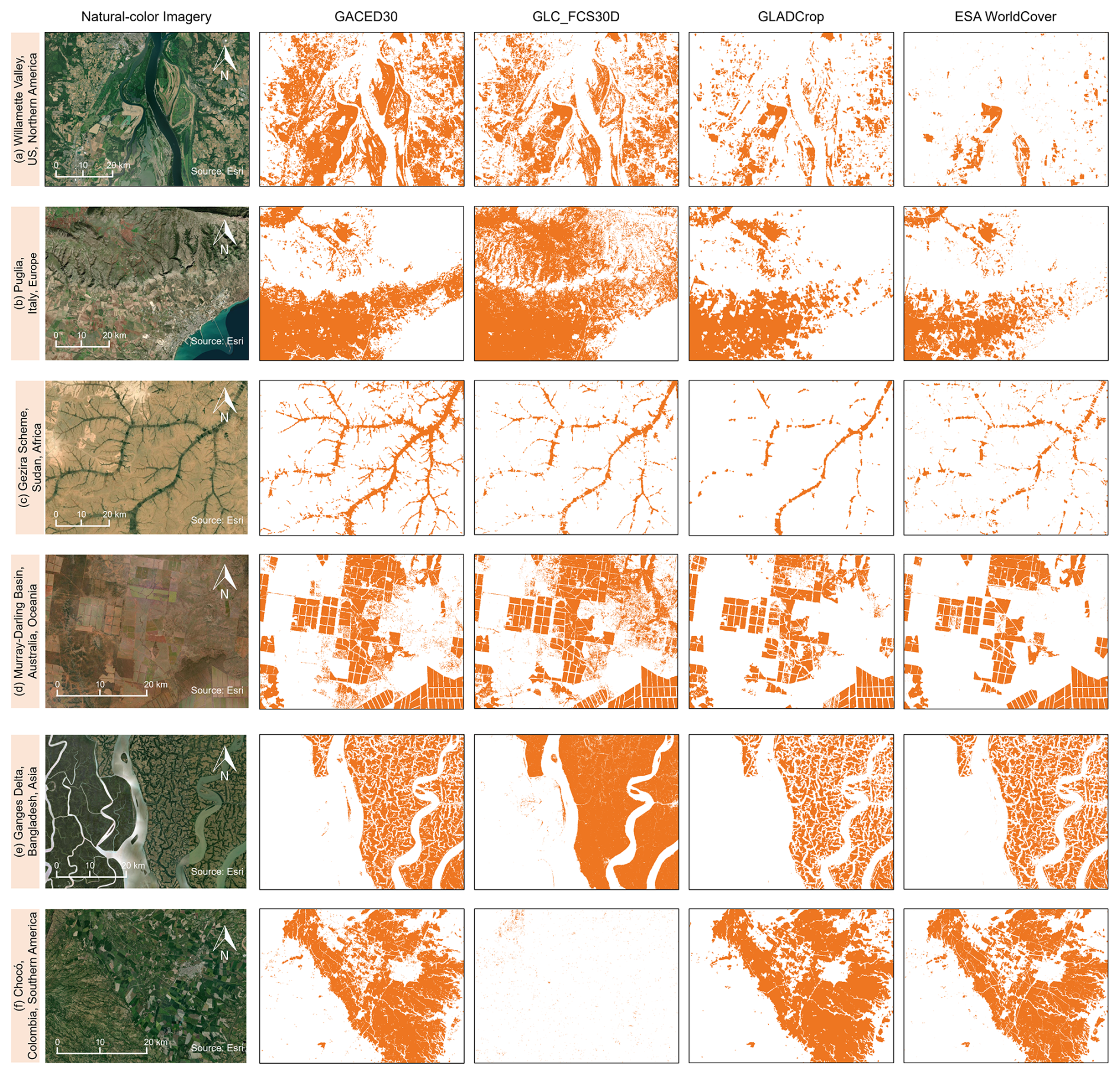
Figure 4 Visual comparison of GACED30 with GLC_FCS30D, GLAD Cropland, and ESA WorldCover across six representative challenging agricultural landscapes. The panels illustrate performance in: (a) Willamette Valley, USA; (b) Puglia, Italy; (c) Gezira Scheme, Sudan; (d) Murray–Darling Basin, Australia; (e) Ganges Delta, Bangladesh; and (f) Chocó Department, Colombia. Background satellite imagery is sourced from Esri World Imagery Wayback (Sources: Esri | Powered by Esri).

In the Willamette Valley, USA (Fig. 4a), the products differ in their representation of managed grass-seed fields that may be spectrally similar to pasture and hay (Mueller-Warrant et al., 2011). Substantial differences are also visible in the drought-prone Murray–Darling Basin, Australia (Fig. 4d), where fallow cropland, pasture, and semi-arid vegetation can be difficult to distinguish (Xie et al., 2024). In Puglia, Italy (Fig. 4b), GACED30 maps broader cropland coverage across the mixed olive-grove and annual-crop landscape than GLAD Cropland, consistent with the inclusion of permanent woody crops in the GACED30 definition (Damianidis et al., 2021). In the Gezira Scheme, Sudan (Fig. 4c), the products differ in their treatment of temporarily bare fields within the irrigated agricultural landscape.

Differences are also apparent in the fragmented paddy and aquaculture landscape of the Ganges Delta, Bangladesh (Fig. 4e), and in the persistently cloud-prone Chocó Department, Colombia (Fig. 4f), where GACED30 produces a comparatively continuous mapped cropland pattern. These examples illustrate how product definitions, observation strategies, and temporal representations affect mapped cropland patterns; quantitative case-level accuracy would require independent reference data.

4.2.2 Characterization of annual cropland dynamics

Whereas Sect. 4.2.1 compares spatial mapping patterns, Fig. 5 illustrates how the annual GACED30 record represents the mapped timing of cropland-status changes. Each panel uses an interval selected to encompass its principal visually evident change episode, and the colours indicate the first year within that interval in which the new status was mapped. This provides a finer temporal description than the multi-year windows available from epoch-based products, although the mapped year should not be treated as an independently verified conversion date.

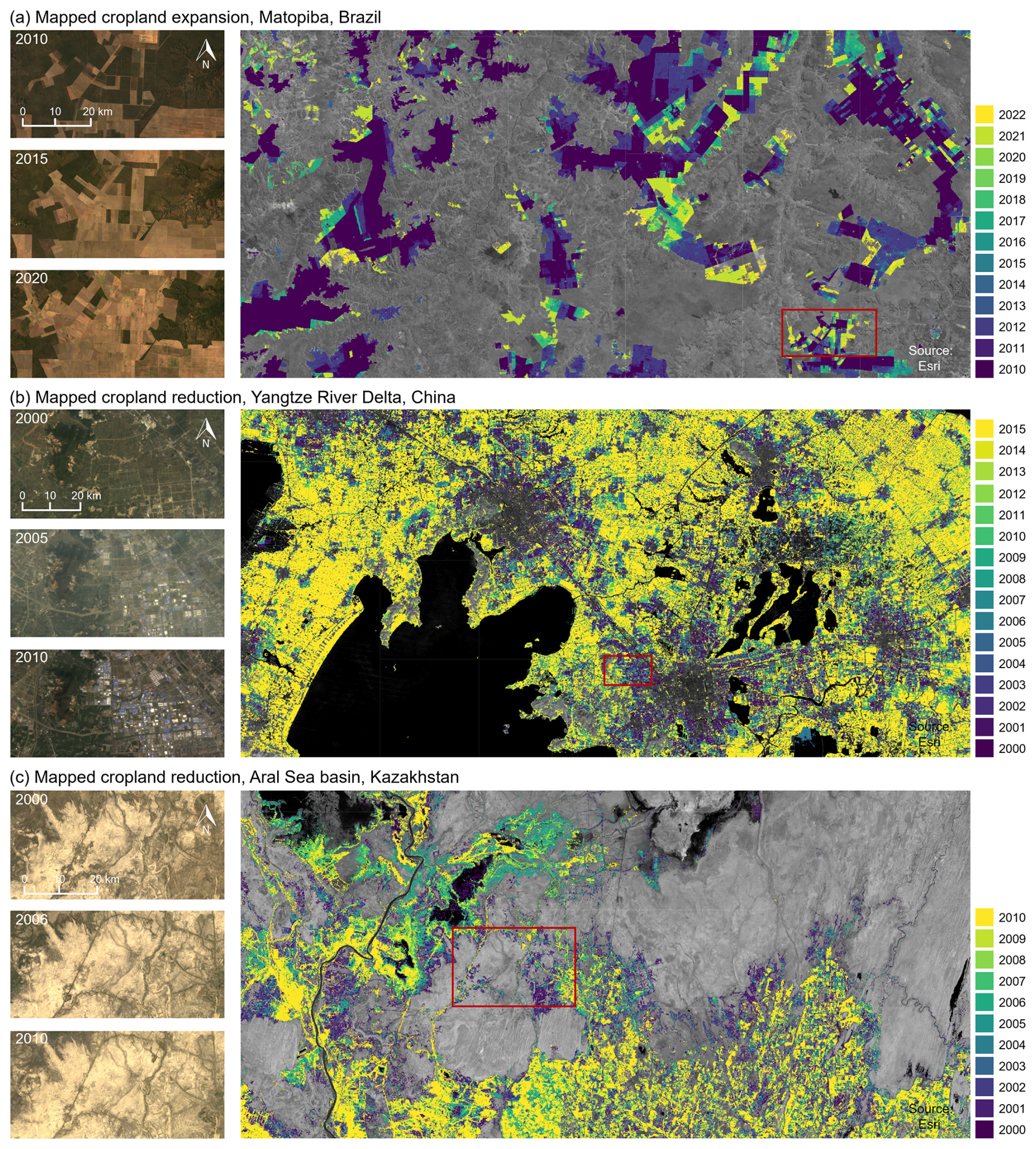
Figure 5 Representative annual cropland-status changes mapped by GACED30 (Sources: Esri | Powered by Esri). Colours denote the first mapped year of the displayed cropland-status transition within each panel-specific interval: (a) cropland expansion in Matopiba, Brazil (2010–2022); (b) cropland reduction in the Yangtze River Delta, China (2000–2015); and (c) cropland reduction in the Aral Sea basin, Kazakhstan (2000–2010). The intervals were selected to encompass the principal visually evident change episode in each case. These examples illustrate the annual temporal information provided by GACED30 and are not intended to verify the cause of change or support quantitative comparisons of change magnitude or timing among regions.

GACED30 depicts the field-scale progression of cropland expansion in Matopiba, Brazil (Fig. 5a), persistent cropland reduction in the peri-urban landscape of the Yangtze River Delta, China (Fig. 5b), and the mapped cessation of cropland status in parts of the Aral Sea basin, Kazakhstan (Fig. 5c). These trajectories can support investigation of potential drivers when combined with independent land-cover, infrastructure, hydrological, soil-salinity, market, and policy information.

4.3 Spatiotemporal dynamics and structural evolution (2000–2024)

4.3.1 Trends in global and regional cropland area

The sample-adjusted GACED30 series estimated global cropland area at 1458.5 Mha (95 % CI: 1428.2–1488.8 Mha) in 2000, 1483.3 Mha in 2020, and 1488.5 Mha (1457.7–1519.3 Mha) in 2024 (Fig. 6a). This represents a net increase of approximately 30.0 Mha, or 2.1 %, from 2000 to 2024, corresponding to an average increase of approximately 1.2 Mha yr⁻¹.

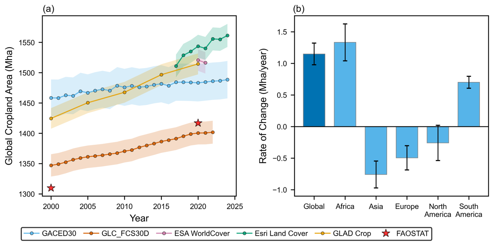
Figure 6 Inter-annual variation and trends in global cropland area from 2000 to 2024. (a) Global cropland-area trajectories from GACED30, GLC_FCS30D, GLAD Cropland, Esri Land Cover, ESA WorldCover, and FAOSTAT. (b) Global and continent-level trends in cropland extent.

The consistently adjusted peer-product series showed different area levels and endpoint changes over their respective periods. GLC_FCS30D increased from 1347.2 Mha in 2000 to 1401.8 Mha in 2022, whereas GLAD Cropland increased from 1424.6 Mha for the 2000–2003 epoch to 1514.5 Mha for the 2016–2019 epoch. Over its shorter temporal coverage, Esri Land Cover increased from 1511.1 Mha in 2017 to 1561.4 Mha in 2024. ESA WorldCover showed little change between its two available years, decreasing from 1520.8 Mha in 2020 to 1516.3 Mha in 2021. The adjusted peer-product series retain substantial differences in both total area and temporal evolution. GACED30 provides a continuous 25-year annual record with a comparatively gradual long-term increase. Across products, the adjusted estimates form a continuum shaped by product-specific mapping behavior and native definitions, particularly their treatment of perennial woody crops, active fallow, temporary meadows and pastures, and mixed agricultural mosaics.

For comparison, the definition-reconciled FAOSTAT estimate was approximately 1417 Mha in 2020, compared with 1483.3 Mha from GACED30, a difference of approximately 66.3 Mha or 4.7 %. In 2020, GACED30 exceeded the definition-reconciled FAOSTAT estimate by 66.3 Mha (4.7 %) but remained within the range spanned by the peer products.

At the continental scale, positive trends were observed in Africa and South America, whereas Asia and Europe showed negative trends (Fig. 6b). The North American trend was slightly negative, but its 95 % confidence interval included zero. The modest global increase therefore reflects opposing regional trajectories rather than uniform worldwide expansion. However, GACED30 alone does not determine the commodity, demographic, policy, or environmental processes responsible for the mapped changes. By emphasizing persistent trends over temporary variability, the analysis indicates that regional expansion frontiers coexist with a relatively stable aggregate global cropland area.

4.3.2 Patterns of cropland persistence and cropping frequency

Beyond static cropland delineation, the annual GACED30 record enables the calculation of cropping frequency (Fig. 7), defined as the proportion of the 25 annual layers in which a pixel was mapped as Cropland. Unlike epoch-based datasets, this annual record directly represents how often each pixel received the Cropland label between 2000 and 2024. In this context, cropping frequency measures the persistence of mapped cropland status – which encompasses both active cultivation and temporary fallow – rather than harvest intensity, such as double or triple cropping. The metric therefore converts the annual binary classifications into a descriptive continuum of mapped persistence.

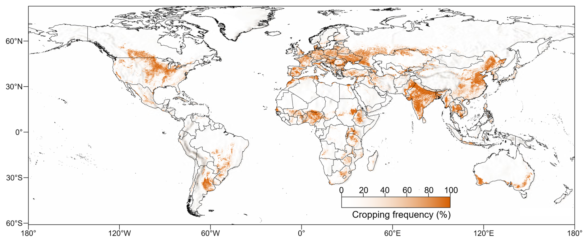
Figure 7 Global spatial distribution of cropping frequency derived from the GACED30 dataset (2000–2024). Pixel values represent the percentage of annual layers in which each pixel was mapped as Cropland, ranging from 0 % (never mapped as Cropland) to 100 % (mapped as Cropland in all 25 years).

Regions exhibiting a cropping frequency approaching 100 % (represented by the darkest orange tones in Fig. 7) delineate areas with persistently mapped cropland status. These areas broadly coincide with established agricultural regions, including the US Corn Belt, the North China Plain, and the Indo-Gangetic Plain. In these core production zones, the high frequency indicates that the corresponding pixels were classified as Cropland in most years under the common annual mapping protocol. Because cropping frequency is derived from the GACED30 classifications themselves, it should be interpreted as a descriptive temporal indicator rather than as independent validation of pixel-level interannual consistency. Conversely, extensive areas in rainfed agricultural regions, particularly the Sahel, Central Asia, and parts of Australia, exhibit intermediate cropping frequencies, typically between 40 % and 70 %. These values may reflect rotational systems, shifting cultivation, land-cover transitions, variable expression of fallow conditions, or residual annual classification variability. They should therefore be interpreted together with the Structural Evolution Indicators and complementary regional evidence.

Low Cropping Frequency values (<30 %) identify pixels classified as Cropland during only a limited part of the 25-year record. Such values can result from recent expansion, earlier cropland reduction, crop rotation or fallow management, or residual annual classification variability and therefore cannot by themselves establish reclamation or abandonment. Their concentration around agricultural margins in regions such as the Brazilian Cerrado, sub-Saharan Africa, eastern Europe, and the Russian Federation identifies locations where Cropping Frequency can be interpreted together with the Structural Evolution Indicators and independent regional evidence.

4.3.3 Spatiotemporal patterns of structural evolution

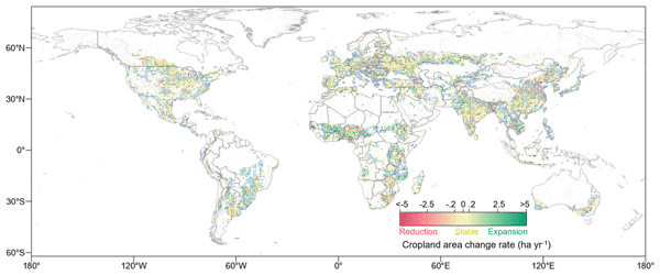
Leveraging the continuous annual time series of GACED30, we quantified global cropland dynamics through grid-level MK and Theil–Sen trend analysis rather than simple bi-temporal differencing. Figure 8a presents both complementary interpretations of the resulting trends: the general structural trend describes all grid cells whose estimated slope exceeds the selected minimum magnitude, whereas the stringent structural trend identifies the subset that additionally satisfies p<0.01. Under the principal threshold of τ=0.2 ha yr⁻¹, stable was the dominant structural-status class, accounting for slightly more than half of the analyzed grid cells; approximately one-quarter were classified as general reduction and slightly more than one-fifth as general expansion (Fig. S1a). Stable cropland was especially extensive in established agricultural regions such as the US Corn Belt, the North China Plain, and Western Europe.

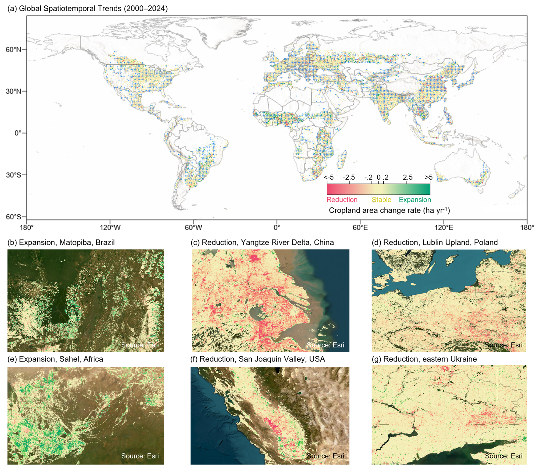
Figure 8 Spatiotemporal patterns of global cropland dynamics from 2000 to 2024. (a) Global distribution of cropland trends aggregated to 1 km grid cells. Grid cells are classified as Expansion (slope>0.2 ha yr⁻¹), Reduction ($\text{slope}<-\mathrm{0.2}$ ha yr⁻¹), or Stable ($\left|\text{slope}\right|\le \mathrm{0.2}$ ha yr⁻¹); blue dots identify grid cells with Mann–Kendall (p<0.01). (b–g) Regional examples of mapped structural change: (b) expansion in Matopiba, Brazil; (c) reduction in the Yangtze River Delta, China; (d) reduction in the Lublin Upland, Poland; (e) expansion in the Sahel; (f) reduction in the San Joaquin Valley, USA; and (g) reduction in eastern Ukraine. Background satellite imagery is sourced from Esri World Imagery Wayback (June 2020) (Sources: Esri | Powered by Esri). National administrative boundaries are sourced from the Resources and Environmental Science Data Platform.

Because τ is an operational rather than theoretically optimal threshold, we examined whether the principal geographical interpretation depended strongly on its selected value. Increasing τ from 0.10 to 0.50 ha yr⁻¹ progressively reassigned lower-magnitude expansion and reduction grid cells to stable, as expected, and therefore changed the absolute mapped extent of structural change (Fig. S1a). However, the continental composition of the general expansion and reduction areas changed only modestly across the evaluated thresholds, with no abrupt redistribution around τ=0.2 ha yr⁻¹ (Fig. S1b and c). Spatial agreement with the τ=0.2 reference masks was also high for nearby thresholds under both definitions: at τ=0.15 and 0.25, the Jaccard indices were approximately 0.88–0.91 for the general masks and 0.91–0.93 for the stringent masks (Fig. S2). Thus, the precise extent of lower-magnitude change remains threshold-dependent, but the broad continental distribution and principal spatial patterns are retained across reasonable values surrounding τ=0.2. Together with the regional patterns in Fig. 8, this supports the robustness of the central interpretation that agricultural expansion is disproportionately concentrated in the Global South, whereas widespread stability and localized contraction characterize much of the Global North. Nevertheless, the sensitivity results do not imply that τ=0.2 is a uniquely optimal threshold.

Under the stringent structural-evolution definition, statistically supported expansion was concentrated in several agricultural-frontier regions of the Global South, including Matopiba in Brazil and parts of the African Sahel (Fig. 8b and e). Persistent reduction was mapped in the Yangtze River Delta, the San Joaquin Valley, the Lublin Upland, and eastern Ukraine (Fig. 8c, d, f, and g). These regional examples were selected to represent contexts in which commodity agriculture, smallholder extensification, urban expansion, groundwater constraints, afforestation or land abandonment, and armed conflict may contribute to cropland change. Such processes provide hypotheses for interpreting the mapped patterns, but causal attribution requires independent land-cover, environmental, socioeconomic, and policy evidence.

Comparison with the GLAD Cropland change maps shows both broad agreement and systematic differences between the two analytical approaches. Both products identify major expansion frontiers in South America and Africa, whereas larger discrepancies occur in semi-arid and transitional regions such as Central Asia and Australia. GLAD represents crop gain and crop loss between adjacent four-year epochs, while the GACED30 Structural Evolution Indicator identifies persistent monotonic trends across the complete annual record under specified slope and significance criteria. Consequently, a change detected within an individual GLAD epoch interval may not produce a statistically supported monotonic trend over the complete 2000–2024 GACED30 record. The products therefore offer complementary representations: GLAD characterizes changes between consecutive multi-year epochs, whereas GACED30 delineates persistent structural trends across the full annual series.

5 Discussion

5.1 From static mapping to structural evolution: Advantages and uncertainties

GACED30 extends global cropland monitoring beyond isolated snapshots by providing annual maps generated under a common observation framework, cropland definition, feature representation, sample-construction procedure, and model configuration. The gap-free SDC30 record supports comparable representation of annual phenological signals, while spectral-semantic alignment expands the geographical coverage of the expert-annotated FAST-Crop samples. The annual classifiers are nevertheless trained independently, and temporal linkage is introduced only through the rotation rule for uncertain one-year observations. GACED30 should therefore be regarded as a harmonized annual baseline rather than an explicitly constrained temporal sequence in which every local transition is enforced.

The complete annual record supports two complementary descriptions of cropland dynamics. Cropping Frequency summarizes the proportion of years in which a pixel was mapped as Cropland, whereas the Structural Evolution Indicators use annual grid-level cropland area, the Mann–Kendall test, and Theil–Sen slopes to identify persistent directional patterns. Analysis of the full trajectory reduces sensitivity to the selection of individual endpoint years, but the exact spatial extent of expansion and reduction remains dependent on the minimum slope threshold. The sensitivity analysis indicates that the broad continental distribution is retained across thresholds near τ=0.2 ha yr⁻¹, although mapped extent remains threshold-dependent and causal interpretation requires additional evidence.

The complementary evaluations describe different aspects of product performance. The FAST-Crop assessment indicates strong static thematic agreement, the matched China assessment shows overall accuracy comparable with CACD, and the AEZ-stratified results identify geographically heterogeneous performance. The GLAD Cropland and LUCAS assessments provide direct evidence on crop-gain and crop-loss detection across multiple intervals: GACED30 achieved higher recall and F₁ than GLC_FCS30D on the common samples, although the modest absolute scores demonstrate the continuing difficulty of transition mapping. Together, these evaluations support global and regional structural monitoring while indicating greater uncertainty in local transition timing.

Differences among the adjusted inter-product trajectories should also be interpreted in relation to product definitions and mapping strategies. GACED30 includes permanent woody crops and active fallow while excluding temporary meadows and pastures, and its GLAD-conditioned augmentation changes the representation of individual cropland subclasses. The global and regional trajectories are therefore specific to the adopted cropland definition and trend criteria.

5.2 Implications for global sustainability and Earth system modelling

The results in Sects. 4.3.1–4.3.3 indicate that global cropland increased modestly from 1458.5 Mha in 2000 to 1488.5 Mha in 2024, while stable cropland remained predominant and statistically significant expansion and reduction were spatially concentrated. This combination shows that a relatively small global net change can coexist with substantial regional reorganisation, particularly the contrast between concentrated expansion in parts of Africa and South America and widespread stability or reduction in much of the Global North. When combined with crop-type maps, yield and production statistics, population, market-access, and nutrition data, GACED30 can contribute the land-extent component of food-security assessments and help distinguish production changes accompanied by cropland expansion from those occurring without marked extent change. The significant trend layer can also identify candidate agricultural-frontier and persistent cropland-reduction zones for targeted monitoring; determining the preceding land cover and environmental implications requires independent forest, grassland, biodiversity, protected-area, infrastructure, and land-tenure information. When combined with trade-flow and socioeconomic data, these spatial trajectories can support telecoupled land-system analyses linking distant production and consumption regions; when paired with policy boundaries, implementation dates, and an appropriate comparison or counterfactual design, they can also serve as an outcome layer for land-use policy evaluation.

Cropland extent is also a fundamental input to irrigation mapping. LANID uses cropland masks to constrain annual irrigation classification, while CIrrMap250 identifies cropland-mask uncertainty as a source that can propagate into irrigation estimates (Xie et al., 2021; Zhang et al., 2024a). The annual 30 m GACED30 layers may therefore provide a consistent cropland baseline for future irrigation mapping and help distinguish changes in irrigated area caused by shifts in cropland extent from changes in irrigation status.

The structural trend record also has practical value for carbon accounting and land-use–climate analysis because persistent directional changes can be distinguished from short-term fluctuations under a transparent statistical criterion. Combined with preceding land-cover classes, biomass and soil-carbon stocks, emission factors, and model assumptions, mapped cropland expansion and reduction can provide spatial activity data or stratification for carbon-accounting and sensitivity analyses. At coarser scales, the 2000–2024 record can be aggregated and harmonised with model grids to compare the spatial allocation, direction, and persistence of observed cropland trends with land-use inputs or outputs used by Earth system models, including LUH2 (Hurtt et al., 2020). Such comparisons can support evaluation of land-use inputs and model behavior; complete land-use forcing additionally requires data on crop types, pasture, management, and transitions among non-cropland classes.

5.3 Limitations and future work

The principal spatial and semantic limitations of GACED30 arise from its binary class structure and 30 m spatial resolution. Active cultivation and rotational fallow are represented within a single Cropland class, so the dataset does not distinguish their annual management status. Fields smaller than or comparable to a Landsat pixel may be omitted or spatially smoothed, particularly in fragmented smallholder landscapes. Temporary fallow, ploughed pasture, degraded rangeland, and natural bare or sparsely vegetated surfaces can also exhibit similar spectral and phenological characteristics. The AEZ assessment illustrates this geographical heterogeneity: in the cool, humid tropical stratum, the producer's accuracy of 0.498 indicates substantial cropland omission despite a high overall accuracy. The boreal sub-humid and humid reference subsets contained no positive Cropland cases and therefore did not support class-specific evaluation. Local applications in these environments require additional regional validation.

Temporal comparability is supported by the common observation, feature, sample-construction, and model protocols, but complete pixel-level interannual consistency is not enforced. The independently trained annual classifiers can remain sensitive to annual spectral conditions, particularly near the classification threshold or during abrupt land-cover changes. Differences between the earlier Landsat–MODIS observation environment and the more recent sensor era may also influence temporal comparability and are not eliminated solely by trend analysis. Moreover, the available GLAD Cropland and LUCAS references assess crop gain and crop loss across multi-year intervals rather than every annual layer. They cannot identify the exact transition year, detect all within-interval reversals, or distinguish permanent cropland reduction from temporary non-cropland states. More independent annual and transition-specific reference observations are therefore needed.

The augmented Cropland layer also retains the influence of the GLAD Cropland spatial prior. Because GLAD Cropland excludes some categories included in GACED30, permanent woody crops and agricultural structures were represented primarily by the FAST-Crop tier and accounted for approximately 3 % of the final combined Cropland training set. The ablation experiment indicated that the effects of augmentation varied among FAST-Crop subclasses, including a small decrease in Orchard performance. Strong binary cropland accuracy should therefore not be interpreted as demonstrating equally well-constrained performance for every cropland subtype.

Future cropland products could integrate 10 m imagery and intra-annual phenology to map finer crop and management categories, complex planting patterns such as multiple cropping, rotations, and intercropping, and individual field boundaries. These advances would improve the representation of small and fragmented fields and extend monitoring beyond binary annual extent.

6 Code and data availability

The Global 30 m Annual Cropland Extent Dynamics (GACED30) dataset generated in this study is openly available from Zenodo at https://doi.org/10.5281/zenodo.18199675 (Chen et al., 2026). Each annual raster layer follows the FROM-GLC coding convention, in which a value of 10 denotes cropland and a value of 0 denotes non-cropland. The SDC30 data cube and the FAST-Crop sample set, which were used as the core input and reference datasets for GACED30 generation and validation, are available at https://data-starcloud.pcl.ac.cn/ (last access: 22 September 2026).

7 Conclusion

This study presents GACED30, to our knowledge the first dedicated global 30 m annual cropland-extent dataset spanning 2000–2024. By combining gap-free SDC30 observations with spectral-semantic sample alignment and a common annual mapping protocol, GACED30 provides a harmonized record of cropland extent from which Cropping Frequency and grid-level Structural Evolution Indicators can be derived. Independent stable-site validation yielded an overall accuracy of 0.965 and an F1 score of 0.844; in the matched China assessment, GACED30 achieved OA, UA, PA, and F1 scores of 0.946, 0.838, 0.843, and 0.840, respectively, comparable to CACD. Multitemporal assessments yielded higher recall and F₁ scores than GLC_FCS30D for both crop gain and crop loss; however, the modest absolute transition scores indicate that local annual changes should be interpreted cautiously. GACED30 estimated global cropland area at 1488.5 Mha in 2024, approximately 30.0 Mha higher than in 2000. The annual trajectory indicates that this modest global net increase comprises contrasting regional patterns, with persistent expansion concentrated in parts of Africa and South America and stability or reduction more widespread across much of the Global North. GACED30 therefore provides a high-resolution annual baseline for monitoring cropland-extent dynamics and for integration with complementary environmental, agricultural, and socioeconomic information.