Signal-domain guided deep learning for gap-filling of XCO and XCH₄: a masked spatio-temporal fusion of TROPOMI and GEOS-Chem (2019–2023)

Long-term, high-resolution monitoring of carbon monoxide (CO) and methane (CH₄) is essential for understanding their spatiotemporal variability and supporting climate mitigation strategies. However, satellite observations from instruments such as the TROPOspheric Monitoring Instrument (TROPOMI) are often spatially and temporally incomplete, while existing fusion methods still struggle to achieve both high accuracy and spatiotemporal continuity. Here, we propose a signal-domain fusion approach that combines three-dimensional discrete cosine transform (3D DCT) and singular value decomposition (SVD) to integrate TROPOMI retrievals with GEOS-Chem simulations. A lightweight residual U-Net is further employed to refine the initial reconstruction by learning residual fields from GEOS-Chem simulations and DCT/SVD reconstruction outputs, guided by a masked loss. The method generates global 0.25° and China-specific 0.05° daily gap-free XCO and XCH₄ datasets from 2019 to 2023. In the time-series comparison analysis at representative sites, the fused datasets generally follow the temporal variations observed by the Total Carbon Column Observing Network (TCCON) and TROPOMI. Missing-rate-threshold experiments further show that the fused products perform comparably to original TROPOMI retrievals under low and moderate missing-rate conditions and show improved performance under sparse TROPOMI coverage (MR >0.5), with R² values of 0.91 for XCO and 0.83 for XCH₄, along with reduced biases and standard deviations. The fused datasets also capture regional XCO increases in parts of North America, decreases over eastern China, and widespread XCH₄ growth, wildfire-related enhancements in Chongqing in 2022, and short-term variations over rice-growing regions. These results indicate that the proposed framework can reconstruct missing satellite observations with improved continuity and provide useful fused datasets for studying regional variability, event-related enhancements, and atmospheric composition changes. The generated datasets are publicly available at https://doi.org/10.5281/zenodo.22010891 (An et al., 2026).

1 Introduction

Carbon monoxide (CO) and methane (CH₄) are two critical atmospheric gases that play a key role in air quality monitoring and climate change research. CO is primarily produced through incomplete combustion of fossil fuels and biomass, as well as the oxidation of CH₄ and other hydrocarbons. Its main sink is the reaction with hydroxyl radicals (OH), which contributes to the formation of tropospheric ozone (O₃) and greenhouse gases such as carbon dioxide (CO₂) (Lelieveld et al., 2016; Spivakovsky et al., 2000). Due to its atmospheric lifetime of weeks to months, CO serves as an effective tracer for pollutant transport, facilitating the study of both horizontal and vertical atmospheric movements (Heald et al., 2003). CH₄ is a powerful greenhouse gas with a significantly longer atmospheric lifespan – around ten years – and a greater global warming potential compared to numerous other gases (Filonchyk et al., 2024; Heilig, 1994). It originates from both natural sources, such as wetlands, permafrost, and wildfires, and anthropogenic activities, including agriculture, livestock digestion, landfills, and fossil fuel extraction (Chai et al., 2016; Jackson et al., 2020). CH₄ plays a crucial role in atmospheric chemistry, influencing the oxidative capacity of the atmosphere and contributing to tropospheric ozone formation. Its rising concentration is a major driver of climate change (Lelieveld et al., 2016).

Although CO and CH₄ are often discussed separately in terms of their sources and impacts, they are chemically and dynamically coupled in the atmosphere. Both gases are predominantly removed by the hydroxyl radical (OH), meaning that changes in one can affect the atmospheric lifetime and concentration of the other through OH competition (Lelieveld et al., 2016). Moreover, they share major emission sources, particularly biomass burning and fossil-fuel-related activities such as incomplete combustion and flaring, where they can be emitted simultaneously (Andreae and Merlet, 2001; Akagi et al., 2011; Andreae, 2019). Their co-emission and co-transport imply that the spatial patterns of CO and CH₄ may be correlated near fire hotspots, industrial regions, and other combustion-influenced areas. Therefore, joint reconstruction of XCO and XCH₄ offers two key advantages: (1) shared spatial structure and common meteorological drivers can provide complementary constraints for deep learning models, improving generalization in data-sparse regions; (2) simultaneous monitoring can support more consistent estimation of emission ratios and source attribution, as demonstrated by studies using CH₄/CO or related trace-gas ratios to constrain biomass-burning and fossil-fuel methane emissions (Worden et al., 2013; Worden et al., 2017; Ramsden et al., 2022). A comprehensive understanding of these coupled gases is fundamental to improving air quality predictions and formulating climate mitigation policies.

Global satellite monitoring enables effective tracking and analysis of the sources, transport, and removal processes of atmospheric pollutants. At present, several satellite instruments provide observations of CO and/or CH₄, including the Measurements of Pollution in the Troposphere (MOPITT), which primarily focuses on CO retrievals (Deeter et al., 2003), as well as the Atmospheric Infrared Sounder (AIRS) (McMillan et al., 2005), Tropospheric Emission Spectrometer (TES) (Rinsland et al., 2006), and Interferometer for the Exploration of the Atmosphere in the Infrared (IASI) (Turquety et al., 2004), which are capable of retrieving multiple trace gases, including CO and CH₄, using different spectral channels and retrieval algorithms. These instruments offer critical data support for the global distribution of CO and CH₄ in the atmosphere.

The TROPOspheric Monitoring Instrument (TROPOMI) onboard the European Space Agency's Sentinel-5P mission provides higher daily global coverage and finer spatial resolution than previous observing missions. According to the official Sentinel-5P/TROPOMI Level-2 product table, the CO and CH₄ products are provided as total column products. In this study, XCO and XCH₄ refer to the column-averaged dry-air mole fractions of atmospheric CO and CH₄, respectively, derived from the corresponding TROPOMI total column products. TROPOMI has already been employed in numerous pertinent applications for XCO and XCH₄ investigations, including the calculation of emissions from biomass combustion (Goudar et al., 2023; Griffin et al., 2024). However, the continuity of TROPOMI atmospheric column retrievals is affected by clouds and aerosols, which can attenuate or scatter the reflected solar radiation measured by satellite sensors. As a result, observations may be incomplete, particularly in regions with high cloud cover and aerosol load – such as the humid tropics and high-latitude zones (Gao et al., 2023), Southeast Asia (Valerio et al., 2025), and eastern China during intense pollution episodes (Wang et al., 2021).

The generation of continuous TROPOMI XCO and XCH₄ products has been addressed through a range of gap-filling approaches. First, machine learning-based interpolation methods (Chen et al., 2022; Hu et al., 2022; Valerio et al., 2025; Wei et al., 2025) reconstruct missing observations by learning nonlinear spatiotemporal relationships. However, their performance strongly depends on the quality and representativeness of the training data, and biased or insufficient samples may lead to unreliable predictions. Second, enhanced spectral fitting algorithms (Borsdorff et al., 2019; Guanter et al., 2015; Schneising et al., 2023; Wang et al., 2020) improve retrieval continuity by refining the spectral inversion process, for example through higher-order polynomial fitting to reduce reflectance-induced biases, albeit at increased computational cost. Third, physics–data–driven coupling approaches, including model fusion, data assimilation, and hybrid machine learning frameworks, integrate satellite retrievals with chemical transport models or reanalysis datasets (Fritz et al., 2022; Schneising et al., 2023; Sicard et al., 2021). By combining physical constraints with data-driven learning or observational corrections, these methods improve spatial consistency and temporal continuity while reducing retrieval bias. However, their performance remains dependent on uncertainties in prior model simulations and the representativeness of assimilated observations (Inness et al., 2022; Wang et al., 2023).

Despite these advances, current methods face challenges in balancing computational efficiency with physical consistency, particularly in regions with persistent cloud cover. To overcome these limitations, this study proposes a novel signal-domain guided spatio-temporal fusion framework. Our core objective is to generate daily global and regional continuous XCO and XCH₄ products (2019–2023) at high resolution (0.25° globally and 0.05° over China) by effectively leveraging complementary information from chemical transport modeling and frequency-domain representations.

The proposed method specifically addresses the shortcomings of existing approaches in three key aspects: (1) Addressing Data Sparsity and Non-linearity: Unlike pure machine learning interpolation that may struggle with unbalanced datasets, we employ a two-stage strategy. We first use 3D Discrete Cosine Transform (DCT) and Singular Value Decomposition (SVD) to perform low-rank signal-domain reconstruction (Rao and Yip, 2014; Wall et al., 2003). This step exploits the shared spatiotemporal structure between GEOS-Chem simulations and TROPOMI observations to approximate missing values in the frequency domain, providing a robust prior; (2) Enhancing Physical Consistency: To correct residual biases without overfitting, we implement a lightweight residual U-Net for pixel-level refinement (Ronneberger et al., 2015; Tang, 2022). Crucially, instead of using the TROPOMI data mask as a direct input feature, we incorporate it as a weighting mask in the loss function (Wei et al., 2022). This masked learning strategy ensures that the model is supervised exclusively by valid observations, thereby preserving the physical consistency of the DCT/SVD-derived signal-domain reconstructed fields; (3) Improving Efficiency and Accuracy: By fusing model-driven priors and observational constraints in both frequency and spatial domains, our method significantly reduces computational load compared to enhanced spectral fitting while avoiding the “black-box” limitation of pure data-driven methods.

Validation against independent TCCON observations demonstrates that the fused outputs outperform GEOS-Chem simulations alone and maintain accuracy comparable to or better than original TROPOMI retrievals in cloud-covered regions. This framework provides an efficient and interpretable solution for large-scale trace gas monitoring and offers new opportunities for atmospheric data assimilation and climate analysis.

2 Measurement and materials

2.1 Data description

2.1.1 TROPOMI XCO and XCH₄ products

This study employs TROPOMI Level-2 data products of column-averaged CO (XCO) and CH₄ (XCH₄). The TROPOMI instrument onboard the Sentinel-5 Precursor (S5P) satellite operates in a polar sun-synchronous orbit, and provides daily global XCO and XCH₄ observations at approximately 13:30 local solar time, thereby enabling near-global daily coverage. The pixel resolution of the TROPOMI XCO and XCH₄ products was improved from 7.0×7.0 km² to 7.0×5.5 km² in June 2019.

TROPOMI retrieves XCO and XCH₄ by measuring Earth-reflected radiation in the shortwave infrared (SWIR) spectral range (2305–2385 nm). For XCO, the retrieval shows high sensitivity to the tropospheric boundary layer under clear-sky conditions; however, this sensitivity is reduced under cloudy conditions due to changes in photon path length and scattering effects (Landgraf et al., 2016). For XCH₄, the operational retrieval algorithm simultaneously estimates column-averaged dry-air mole fractions of CH₄ together with atmospheric scattering parameters. High retrieval accuracy and precision are generally achieved under clear-sky conditions over land after strict filtering of scenes affected by clouds, aerosols, or high surface albedo variability (Hu et al., 2016).

The TROPOMI Level-2 CO and CH₄ products used in this study were obtained from the NASA GES DISC Sentinel-5P/TROPOMI archive for the period 2019–2023. We used the OFFL (Offline) datasets. Specifically, the CO product used is S5P_L2__CO_____HiR, Version 02 (Copernicus Sentinel-5P (processed by ESA), 2021a), while the CH₄ product used is S5P_L2__CH4____HiR, Version 02 (Copernicus Sentinel-5P (processed by ESA), 2021b). These Version 02 products include updated spectroscopic parameters and improved treatments for non-scattering clouds compared with earlier releases. The CO product was converted to XCO, and the CH₄ product is reported as XCH₄. Both XCO and XCH₄ are reported as column-averaged dry-air mole fractions in parts per billion (ppb). To ensure the quality and reproducibility of the satellite observations, we applied product-specific quality screening and retained only TROPOMI retrievals with a quality value (qa_value) greater than 0.5 for subsequent analysis, following the recommended quality-screening threshold for the Sentinel-5P CO and CH₄ Level-2 products.

2.1.2 GEOS-Chem chemical transport model

This study employs the GEOS-Chem model, a global three-dimensional atmospheric chemistry model driven by meteorological input from the Goddard Earth Observing System (GEOS) of the NASA Global Modeling and Assimilation Office (GMAO). We employed version 14.1.1 (https://geoschem.github.io/, last access: 9 September 2026), which is driven by GEOS-FP meteorological data. The most recent GEOS-5 meteorological data product to be provided by NASA/GMAO is GEOS-FP (“forward processing”) (https://geoschem.github.io/overview.html, last access: 9 September 2026). This product has a native horizontal resolution of 0.25° latitude × 0.3125° longitude and a temporal resolution of hourly data and 3-hourly data.

To balance computational cost and regional spatial detail, GEOS-Chem simulations were performed at a 2° × 2.5° horizontal resolution for global simulations, and at a 0.25° × 0.3125° nested resolution for regional simulations over China. The model time steps were set to 300 s for convective and advective transport, and 600 s for chemical processes.

The simulations incorporated detailed region-specific emission inventories. Anthropogenic emissions were sourced from the Air Pollutant Emission Inventory (APEI) v2016 for Canada, the National Emission Inventory (NEI) v2015-03 for North America, DICE-Africa for Africa (Marais and Wiedinmyer, 2016), and the MIX v1.1 inventory combined with HTAP for Asia (Li et al., 2017). Global aircraft and ship emissions were provided by the Community Emissions Data System (CEDS) (Hoesly et al., 2018), while biomass-burning CO emissions were obtained from the Quick Fire Emissions Dataset (QFED) versions 2.1, 2.2, and 2.4.

Based on these inputs and physical processes, GEOS-Chem simulates three-dimensional CO and CH₄ fields. However, XCO and XCH₄ are not direct native outputs; they were diagnosed during post-processing from the simulated vertical profiles. Specifically, the dry-air mole fraction profiles were vertically averaged using pressure-layer thickness as weighting, producing column-averaged dry-air mole fractions consistent with the definitions used by TROPOMI and TCCON. The resulting fields were converted to parts per billion (ppb) for use in the fusion framework.

In the proposed fusion framework, these GEOS-Chem simulations serve as large-scale physical priors. To match the spatial resolution of satellite observations, the global 2° × 2.5° GEOS-Chem fields were regridded to a 0.25° × 0.25° target grid, while the China 0.25° × 0.3125° fields were regridded to a 0.05° × 0.05° target grid. Regridding was performed using inverse distance weighting (IDW) to interpolate GEOS-Chem fields onto the target grids.

2.1.3 Total Carbon Column Observing Network (TCCON) measurements

TCCON employs a Fourier Transform Infrared Spectrometer (FTS) to measure direct solar light in order to determine the total column concentrations of greenhouse gases in the atmosphere, including carbon dioxide (CO₂), CH₄, CO, and others (Buschmann et al., 2016; Kiel et al., 2016; Sha et al., 2020; Yang et al., 2020). These data are extensively utilized to validate satellite remote sensing data (e.g., Chander et al., 2013; Imasu et al., 2023; Lin et al., 2024; Loew et al., 2017; Wu et al., 2019; etc.) and to evaluate the performance of climate models. Due to its high precision, standardized retrieval algorithm, and consistent calibration across sites, TCCON is widely regarded as a primary ground-based reference network for validating satellite greenhouse-gas products (Wunch et al., 2011; Herkommer et al., 2024). They are rigorously calibrated and validated with high accuracy and reliability. TCCON's observing stations are situated in numerous regions worldwide, providing a comprehensive understanding of the global greenhouse gas distribution. These stations are capable of observing a diverse array of climates and ecosystems. Harmonized processing is implemented for each site's data. In order to guarantee data consistency and comparability, the data from each station is processed in a consistent manner. TCCON's XCO and XCH₄ Dry Air Mole Fraction (Xgas) in ppb are employed in this study. Site-specific and time-scale data are accessible through the official website of TCCON (https://tccondata.org/, last access: 9 September 2026), and users may select the data that is most relevant to their research requirements. The validation of XCO and XCH₄ products from TROPOMI and GEOS-Chem is frequently conducted using TCCON (Borsdorff et al., 2019; Cogan et al., 2012; Inness et al., 2022; Schneising et al., 2019).

In this study, we employed the TCCON GGG2020 data release (Laughner et al., 2023), with site-specific datasets accessible through the official TCCON website (https://tccondata.org/2020, last access: 9 September 2026). The TCCON sites used in this study, shown in Fig. S1 and listed in Table S1 in the Supplement, were selected based on data availability during 2019–2023, temporal overlap with the TROPOMI and GEOS-Chem datasets, and geographical representativeness. The selected sites cover broad latitudinal ranges and different environmental conditions, including remote background regions, mid-latitude continental sites, high-latitude regions, island sites, and urban-influenced or emission-affected regions. All stations listed in Table S1 were included in the comprehensive TCCON validation whenever valid collocated samples were available after applying the temporal and spatial matching criteria described in Sect. 3.1. A subset of these stations was additionally selected for representative time-series and scatterplot examples based on data completeness and relatively continuous records; these illustrative examples were not used as the sole basis for the overall validation statistics.

Regarding data filtering, TCCON FTS instruments measure direct solar radiation, and the retrievals are therefore already subject to the network's standard clear-sky retrieval and quality-control procedures. In this study, we applied the standard quality control provided with the TCCON GGG2020 data release and did not impose additional cloud-cover filters on the TCCON measurements. Additional filtering related to satellite data availability, including the TROPOMI missing-rate criterion within the 2° collocation window, is described separately in Sect. 3.1.

2.2 Methodology

In this study, we propose a two-stage fusion framework that integrates physical modeling, signal-domain reconstruction, and deep learning-based residual correction to achieve continuous and accurate global mapping of atmospheric trace gases. The overall workflow is illustrated in Fig. 1, which presents the main components and their interconnections. In the first stage, a signal-domain spatio-temporal reconstruction is employed to exploit the low-frequency consistency and spatio-temporal correlations between the TROPOMI observations and GEOS-Chem simulations, effectively filling missing data regions caused by cloud cover or instrument limitations. In the second stage, a residual learning network based on a lightweight residual U-Net is introduced to refine the fused data by learning nonlinear and region-specific discrepancies between the preliminary reconstruction and the true satellite observations.

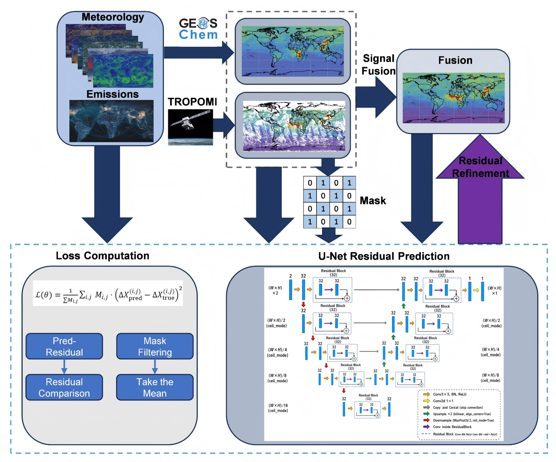
Figure 1 Overview of the proposed fusion framework combining physical modeling, signal-domain reconstruction, and deep learning-based residual correction. The process includes data preprocessing, DCT&SVD-based spatio-temporal fusion, and residual refinement via a lightweight residual U-Net architecture. Arrows indicate the information flow across different modules.

2.2.1 Data preprocessing

Data preprocessing is essential for ensuring the reliability of the fusion results. To reconcile the spatial resolution differences between satellite retrievals and model simulations, TROPOMI XCO and XCH₄ retrievals with qa_value below 0.5 were excluded, and the remaining observations were aggregated onto a global 0.25° × 0.25° grid (720×1440) using area-weighted averaging (Wang et al., 2018). GEOS-Chem outputs were subsequently interpolated to the same grid using inverse distance weighting (Setianto and Triandini, 2013). The 0.25° spatial resolution was selected to balance the representation of mesoscale spatial variability with computational efficiency for multi-year global fusion analyses (Hu et al., 2024; Wang et al., 2023).

To evaluate the influence of the resolution mismatch between GEOS-Chem simulation results and the final fused product, we used the 2019 CO data to conduct a one-year resolution sensitivity experiment. In this experiment, we used GEOS-Chem simulation data at the native 2° × 2.5° resolution and aggregated TROPOMI XCO to the 2° × 2.5° resolution using the area-weighted averaging method. The related fusion calculation framework was directly implemented on the 2° × 2.5° grid; subsequently, the obtained fused XCO data at the 2° × 2.5° resolution were compared with the fused product obtained by aggregating the fused XCO data at the 0.25° resolution to the same 2° × 2.5° grid using the area-weighted averaging method.

2.2.2 Averaging-kernel sensitivity test

We conducted an additional sensitivity test to examine the influence of TROPOMI averaging kernels (AKs) on the comparison between satellite retrievals and model simulations. For 2019, quality-screened TROPOMI CO Level-2 retrievals (qa_value >0.5) were collocated with GEOS-Chem CO vertical profiles. Two GEOS-Chem XCO datasets were then generated for comparison. For the first dataset, GEOS-Chem XCO was diagnosed from the simulated CO profiles by vertically averaging the dry-air mole fractions using pressure-layer thickness as weighting, consistent with the standard post-processing procedure described above. For the second dataset, the GEOS-Chem CO profiles were first interpolated to the TROPOMI pressure layers and then smoothed using the TROPOMI CO column averaging kernels. Finally, both the original GEOS-Chem XCO and the AK-smoothed GEOS-Chem XCO were compared with TROPOMI XCO in ppb.

2.2.3 Spatio-temporal data fusion method based on signal domain reconstruction

Previous studies have shown that emission inventories typically underestimate GEOS-Chem simulation results (Hu et al., 2018; Liang et al., 2023). Despite these magnitude biases, GEOS-Chem simulations generally remain consistent with TROPOMI observations in terms of spatio-temporal variability, exhibiting similar temporal evolution patterns, including concurrent increases and decreases. This consistency suggests that the spatio-temporal correlation between GEOS-Chem simulations and TROPOMI observations can be effectively exploited. By leveraging this relationship, a data fusion framework based on signal-domain reconstruction can be used to generate datasets with improved spatial continuity and more complete coverage (Chen et al., 2022; He et al., 2022; Wang et al., 2021).

We assume that a spatio-temporal relationship exists between the GEOS-Chem simulations and TROPOMI observations for XCO and XCH₄, as expressed below:

$$\begin{array}{}\text{(1)}& \mathrm{XT}=f\left(\mathrm{XG},\mathrm{Lat},\mathrm{Lon},\mathrm{Date}\right)\end{array}$$

where Lat, Lon, and Date denote latitude, longitude, and time, respectively; XG represents the GEOS-Chem XCO and XCH₄ concentration field; and XT represents the corresponding TROPOMI observation field. In other words, the TROPOMI value at a given spatio-temporal coordinate can be approximated using the modeled concentration and its spatial and temporal information.

To simplify the representation of this relationship, Eq. (1) is reformulated as an element-wise scaling of the GEOS-Chem field by a spatio-temporal transformation matrix ρ:

$$\begin{array}{}\text{(2)}& \mathrm{XT}=\mathrm{XG}\cdot \mathit{\rho }\end{array}$$

where ⋅ denotes element-wise multiplication, also known as the Hadamard product. The matrix ρ represents the local spatio-temporal relationship between GEOS-Chem and TROPOMI at each grid cell and time step. It has the same dimensions as XT and XG. Known values of ρ can be obtained at valid TROPOMI pixels by comparing XT and XG, while missing values of ρ need to be reconstructed.

The parameter matrix ρ is assumed to be smooth in space and time, inspired by previous studies on filling missing values in spatio-temporal data and enhancing data smoothness using multidimensional discrete cosine transforms (Elharar et al., 2007; Garcia, 2010; Robinson and Kecman, 2003; Okolie and Smit, 2022; Peng et al., 2005; Rao and Yip, 2014; Wang et al., 2023). We therefore propose a spatio-temporal 3D matrix smoothing algorithm based on the discrete DCT and SVD to enhance data smoothness and fill missing values in spatio-temporal data. The method effectively handles spatio-temporal data with missing values while maintaining spatio-temporal correlation by combining spatio-temporal nearest-neighbor interpolation and regularized optimization techniques.

We find the spatio-temporal 3D matrix $\widehat{\mathit{\rho }}$ that minimizes Eq. (3) by means of the 3D DCT. The objective function includes the residual term on the left-hand side and the smoothing term on the right-hand side:

$$\begin{array}{}\text{(3)}& E\left(\widehat{\mathit{\rho }}\right)=\left|\right|{\mathit{\omega }}^{\frac{\mathrm{1}}{\mathrm{2}}}\cdot (\widehat{\mathit{\rho }}-\mathit{\rho })|{|}^{\mathrm{2}}+\mathit{ϵ}|\left|{\mathrm{\nabla }}^{\mathrm{2}}\widehat{\mathit{\rho }}\right|{|}^{\mathrm{2}}\end{array}$$

where $\left|\right|\cdot \left|\right|$ denotes the Euclidean paradigm, ω is a binary mask indicating the availability of a parameter corresponding to the spatio-temporal location of ρ, ϵ denotes the smoothing parameter, and ∇² denotes the Laplace operator. The satisfied condition $\widehat{\mathit{\rho }}$ can be solved by iteration of Eq. (4):

$$\begin{array}{}\text{(4)}& \widehat{\mathit{\rho }}=\mathit{\alpha }{\mathrm{IDCT}}_{\mathrm{3}}\left({\mathrm{\Gamma }}^{\mathrm{3}}\cdot {\mathrm{DCT}}_{\mathrm{3}}\left(\mathit{\omega }\cdot \left(\mathit{\rho }-\widehat{\mathit{\rho }}\right)+\widehat{\mathit{\rho }}\right)\right)+\left(\mathrm{1}-\mathit{\alpha }\right)\widehat{\mathit{\rho }}\end{array}$$

where α is a parametric factor for accelerating convergence, Γ³ denotes the 3D spatio-temporal filtering matrix associated with the smoothing term, which can be obtained through Eq. (5), and DCT₃ and IDCT₃ denote the 3D discrete cosine signal transform and its inverse transform, respectively.

$$\begin{array}{}\text{(5)}& {\mathrm{\Gamma }}_{i_{\mathrm{1}},i_{\mathrm{2}},i_{\mathrm{3}}}^{\mathrm{3}}={\displaystyle \frac{\mathrm{1}}{\mathrm{1}+\mathit{ϵ}{\sum }_{k=\mathrm{1}}^{\mathrm{3}}\mathrm{2}\left[\mathrm{1}-\cos \frac{(i_k-\mathrm{1})\mathit{\pi }}{n_k}\right]}}\end{array}$$

Here, i_k denotes the i-th value along the k-th dimension and n_k denotes the size of ρ along the k-th dimension. This means that the value at each position of this three-dimensional spatio-temporal filtering matrix is completely determined by its position. The closer its position is to the element at position (1, 1, 1), the larger (the closer it is to 1) the value is, and vice versa. The value at position (1, 1, 1) is 1. Since the low-frequency components of the discrete cosine transformed signal matrix are mainly located close to position (1, 1, 1), this filtering matrix allows us to search for a smoothed ρ in the frequency domain. In this study, the total number of iterations is empirically set to 100, α is set to 0.75, and ϵ is selected through an automated search within 10⁻³ to 10⁻¹, using the value that minimizes the reconstruction error on valid observations. This optimization is performed independently for XCO and XCH₄ and for the global and China domains.

Equations (6) and (7) define the forward and inverse three-dimensional discrete cosine transforms used in the iterative update in Eq. (4). Specifically, DCT₃ transforms the spatio-temporal parameter matrix ρ from the latitude–longitude–time domain into the frequency domain, where the dominant large-scale and slowly varying structures are represented by low-frequency coefficients. After the smoothing filter Γ³ in Eq. (5) is applied to these coefficients, IDCT₃ transforms the filtered signal back to the original spatio-temporal domain. Therefore, Eqs. (6) and (7) provide the mathematical basis for the frequency-domain smoothing and reconstruction of ρ.

The 3D DCT, denoted as DCT₃, is defined as:

$$\begin{array}{}\text{(6)}& \begin{array}{rl}F(u,v,w)& ={\displaystyle \frac{\mathrm{2}}{\sqrt{\mathrm{NMP}}}}{\sum }_{x=\mathrm{0}}^{N-\mathrm{1}}{\sum }_{y=\mathrm{0}}^{M-\mathrm{1}}{\sum }_{z=\mathrm{0}}^{P-\mathrm{1}}\\ f(x,y,z)& \cos \left({\displaystyle \frac{\mathit{\pi }(\mathrm{2}x+\mathrm{1})u}{\mathrm{2}N}}\right)\cos \left({\displaystyle \frac{\mathit{\pi }(\mathrm{2}y+\mathrm{1})v}{\mathrm{2}M}}\right)\\ & \cos \left({\displaystyle \frac{\mathit{\pi }(\mathrm{2}z+\mathrm{1})w}{\mathrm{2}P}}\right)\end{array}\end{array}$$

where $u=\mathrm{0},\mathrm{1},\mathrm{2},\mathrm{\dots },N-\mathrm{1}$, $v=\mathrm{0},\mathrm{1},\mathrm{2},\mathrm{\dots },M-\mathrm{1}$, and $w=\mathrm{0},\mathrm{1},\mathrm{2},\mathrm{\dots },P-\mathrm{1}$. N, M, and P represent the size of the signal in each of the three dimensions.

The inverse 3D DCT, denoted as IDCT₃, is defined as:

$$\begin{array}{}\text{(7)}& \begin{array}{rl}f(x,y,z)& ={\displaystyle \frac{\mathrm{2}}{\sqrt{\mathrm{NMP}}}}{\sum }_{u=\mathrm{0}}^{N-\mathrm{1}}{\sum }_{v=\mathrm{0}}^{M-\mathrm{1}}{\sum }_{w=\mathrm{0}}^{P-\mathrm{1}}\\ F(u,v,w)& \cos \left({\displaystyle \frac{\mathit{\pi }(\mathrm{2}x+\mathrm{1})u}{\mathrm{2}N}}\right)\cos \left({\displaystyle \frac{\mathit{\pi }(\mathrm{2}y+\mathrm{1})v}{\mathrm{2}M}}\right)\\ & \cos \left({\displaystyle \frac{\mathit{\pi }(\mathrm{2}z+\mathrm{1})w}{\mathrm{2}P}}\right)\end{array}\end{array}$$

where $x=\mathrm{0},\mathrm{1},\mathrm{2},\mathrm{\dots },N-\mathrm{1}$, $y=\mathrm{0},\mathrm{1},\mathrm{2},\mathrm{\dots },M-\mathrm{1}$, and $z=\mathrm{0},\mathrm{1},\mathrm{2},\mathrm{\dots },P-\mathrm{1}$. N, M, and P represent the size of the signal in each of the three dimensions. Through the repeated application of DCT₃ frequency-domain filtering, and IDCT₃, missing values in ρ can be reconstructed while preserving the dominant low-frequency spatio-temporal structure.

Furthermore, the 3D discrete cosine transform requires a complete 3D matrix for signal conversion. Consequently, we first interpolate ρ with missing values using the spatio-temporal autocorrelation property of ρ. Subsequently, SVD is applied to retain the dominant components of the reconstructed parameter matrix and reduce weak noisy components. In this study, 80 % of the cumulative singular-value energy is retained as a practical and computationally efficient truncation threshold for the preliminary reconstruction. The rule of SVD is illustrated in Eq. (8), which is used to preserve the primary components of ρ for the iteration in Eq. (4):

$$\begin{array}{}\text{(8)}& \mathbf{A}=\mathbf{U}\mathbf{\Sigma }{\mathbf{V}}^T\end{array}$$

where $\mathbf{A}\in {\mathbb{R}}^{m\times n}$, $\mathbf{U}\in {\mathbb{R}}^{m\times m}$ are orthogonal matrices whose column vectors are called left singular vectors; $\mathbf{\Sigma }\in {\mathbb{R}}^{m\times n}$ is a diagonal matrix whose diagonal elements are the singular values ${\mathit{\sigma }}_{\mathrm{1}}\ge {\mathit{\sigma }}_{\mathrm{2}}\ge \mathrm{\cdots }\ge {\mathit{\sigma }}_r\ge \mathrm{0}$, and r is the rank of the matrix A. $\mathbf{V}\in {\mathbb{R}}^{n\times n}$ is an orthogonal matrix whose column vectors are called right singular vectors.

To evaluate whether this empirical threshold materially affects the reconstruction, we conducted an additional threshold-sensitivity experiment for the 2019 daily global XCO reconstruction. Daily GEOS-Chem XCO simulations and collocated TROPOMI CO retrievals on the 0.25° × 0.25° grid were used to construct the TROPOMI/GEOS-Chem ratio fields. The same DCT-SVD reconstruction procedure was repeated using cumulative singular-value energy thresholds of 70 %, 75 %, 80 %, 85 %, 90 %, and 95 %, with the 80 % case used as the reference. The results are summarized in Table S8 and Fig. S2.

Calculate the total energy of the singular values as $E_{\mathrm{total}}={\sum }_{i=\mathrm{1}}^r{\mathit{\sigma }}_i^{\mathrm{2}}$, and find the smallest k such that the first k singular values account for at least 80 % of the total energy, i.e., $\left({\sum }_{i=\mathrm{1}}^k{\mathit{\sigma }}_i^{\mathrm{2}}\right)/E_{\mathrm{total}}\ge \mathrm{0.8}$. Then, setting the last r–k smaller singular values in Σ to zero yields the truncated diagonal matrix ${\mathbf{\Sigma }}_k=\mathrm{diag}({\mathit{\sigma }}_{\mathrm{1}},{\mathit{\sigma }}_{\mathrm{2}}\mathrm{\dots },{\mathit{\sigma }}_k,\mathrm{0},\mathrm{\dots },\mathrm{0})$. Finally, reconstruct the approximation matrix using the truncated singular value matrix A_k=UΣ_kV^T.

2.2.4 Deep residual refinement via learning-based mask reconstruction

To further enhance the reconstruction quality, we introduced a residual learning module based on a deep neural network to refine the preliminary DCT/SVD reconstruction. Although the signal-domain reconstruction captures the dominant spatiotemporal structures shared by GEOS-Chem and TROPOMI, local nonlinear discrepancies may still remain because of retrieval noise, regional emission variability, transport errors, and meteorological influences. Therefore, a residual U-Net was employed to learn pixel-level corrections between the preliminary fused field and valid TROPOMI observations.

Because the target grids are finer than the native GEOS-Chem grids, the residual-learning step should be interpreted as observation-constrained reconstruction rather than pure model downscaling. GEOS-Chem provides the large-scale physical background, while the residual network learns corrections between the preliminary DCT/SVD reconstruction and valid TROPOMI observations on the target grid. Therefore, fine-scale variations in the fused datasets are constrained primarily by satellite-observed spatial patterns and auxiliary meteorological information, rather than being generated solely from the coarse GEOS-Chem fields.

Residual learning objective

Let X_DCT denote the preliminary fused XCO/XCH₄ field obtained from the DCT/SVD-based reconstruction, and X_TROPOMI be the valid observational values from the satellite. The residual between the fusion estimate and the true value (only available at observed locations) is defined as:

$$\begin{array}{}\text{(9)}& \mathrm{\Delta }{X}_{\mathrm{true}}=X_{\mathrm{TROPOMI}}-X_{\mathrm{DCT}},\mathrm{where}\mathbf{M}=\mathrm{1}\end{array}$$

Here, $\mathbf{M}\in \mathit{\{}\mathrm{0},\mathrm{1}{\mathit{\}}}^{H\times W}$ is a binary mask indicating the presence (1) or absence (0) of valid satellite data. The goal is to train a model ℱ_θ(⋅) parameterized by θ to predict the residual ΔX_pred across the entire domain:

$$\begin{array}{}\text{(10)}& \mathrm{\Delta }{X}_{\mathrm{pred}}={\mathcal{F}}_{\mathit{\theta }}(X_{\mathrm{G}},X_{\mathrm{DCT}},\mathbf{A})\end{array}$$

where X_G denotes the GEOS-Chem full-coverage simulation data; X_DCT denotes the DCT/SVD-reconstructed preliminary fusion; A denotes the auxiliary information such as meteorological fields and emission inventories. Precursor meteorological data simulated by GEOS-Chem and emission inventory were used in this study. The final fused data is obtained by correcting the DCT/SVD estimate with the predicted residual:

$$\begin{array}{}\text{(11)}& X_{\mathrm{fused}}=X_{\mathrm{DCT}}+\mathrm{\Delta }{X}_{\mathrm{pred}}\end{array}$$

Loss function design

The model is trained using only the valid observations, i.e., locations where M=1. The masked loss was used because reliable TROPOMI targets are available only at valid retrieval pixels; pixels affected by clouds, aerosols, or retrieval failures do not provide trustworthy reference values. The mask therefore avoids penalizing the network at invalid or missing satellite pixels. Although the loss is computed only at valid pixels, the trained residual model is applied to the full spatial domain because its inputs, including GEOS-Chem simulations and the preliminary DCT/SVD reconstruction, are spatially complete or reconstructed before residual learning. Thus, the model transfers residual relationships learned from valid observations to missing regions with similar spatiotemporal patterns represented by the two input fields, following the logic of recent masked-learning atmospheric gap-filling studies (Wei et al., 2023; Sun et al., 2026). The loss function is designed to minimize the residual error at these observed locations:

$$\begin{array}{}\text{(12)}& \mathcal{L}\left(\mathit{\theta }\right)={\displaystyle \frac{\mathrm{1}}{\sum M_{i,j}}}{\sum }_{i,j}{M}_{i,j}\cdot {\left(\mathrm{\Delta }{X}_{\mathrm{pred}}^{(i,j)}-\mathrm{\Delta }{X}_{\mathrm{true}}^{(i,j)}\right)}^{\mathrm{2}}\end{array}$$

This masked mean squared error ensures that the learning focuses on valid TROPOMI retrievals. However, because valid retrievals may be spatially or temporally clustered in cloud-free regions, the masked loss may introduce sampling bias and affect extrapolation in persistently cloudy or aerosol-affected areas where valid observations are sparse. This risk is partly mitigated by the use of spatially complete predictors, including GEOS-Chem simulations and the preliminary DCT/SVD reconstruction, which provide physical and spatiotemporal constraints across the full domain. Nevertheless, fused data in regions with persistent data gaps should be interpreted with caution.

Model architecture and training

In this study, we employed a lightweight residual U-Net architecture to predict the full-domain residual field ΔX_pred, which represents the correction from the DCT/SVD reconstruction to the expected TROPOMI observation. The network inputs include two channels: the GEOS-Chem simulation and the DCT/SVD reconstruction output (Wang et al., 2025). The TROPOMI mask is not used as an input but is instead applied during the loss computation to focus learning only on valid pixels.

The residual U-Net consists of an encoder–decoder structure with skip connections and lightweight residual blocks. The network contains 10 convolutional layers in total, including the convolutional layers inside the residual blocks. All hidden convolutional layers use 32 filters, with two input channels and one output channel for the predicted residual field. The input and output spatial dimensions remain unchanged (i.e., 720×1440 at 0.25° resolution), enabling pixel-wise learning of spatial residuals. The model was trained using daily global maps from 2019 to 2023. Training was performed for 5 epochs with a batch size of 4. We used the Adam optimizer with a fixed learning rate of $\mathrm{1}\times {\mathrm{10}}^{-\mathrm{4}}$, and no learning-rate scheduler was applied. No dropout layer or data augmentation was used in the final configuration. To improve numerical stability, all input variables were normalized before training. The final output is truncated to avoid physically implausible corrections, by enforcing:

$$\begin{array}{}\text{(13)}& \left|\mathrm{\Delta }{X}_{\mathrm{pred}}\right|<\mathit{\gamma }\cdot {\mathit{\sigma }}_{\mathrm{TROPOMI}},\mathit{\gamma }=\mathrm{3}\end{array}$$

where σ_TROPOMI denotes the standard deviation of observed valid values, and γ is a hyperparameter controlling confidence bounds. This truncation is applied only to the neural-network-predicted residual correction, not directly to the final XCO or XCH₄ concentration fields. Its purpose is to prevent unphysical residual corrections arising from unstable extrapolation in regions with sparse valid TROPOMI observations. We acknowledge that such truncation may partly dampen extremely large residual corrections and could therefore reduce the magnitude of rare local extremes. However, because the truncation is imposed on the residual term rather than on the full concentration fields, the large-scale and physically consistent extreme signals already present in the GEOS-Chem simulations, TROPOMI observations, or DCT/SVD reconstruction are retained. Thus, the constraint mainly suppresses anomalous correction spikes while preserving the dominant extreme-event signals.

2.2.5 Ablation study design

To explicitly isolate the contribution of each component in the proposed two-stage framework, we conducted an ablation study using site-based validation across all TCCON stations for the year 2021. Five configurations were compared: (1) only DCT fusion (Garcia, 2010), (2) DCT and SVD mixed-signal reconstruction (Bengherabi et al., 2008; Majhi and Pal, 2021), (3) residual CNN (Jiang et al., 2024), (4) residual U-Net (Ronneberger et al., 2015; Yan et al., 2022), and (5) residual XGBoost (Naseem et al., 2024). The performance was assessed using the coefficient of determination (R²), root mean square error (RMSE), and mean bias (μ). This design allows the contribution of the DCT/SVD signal-domain reconstruction stage and the residual-correction stage to be evaluated separately. The site-based validation results are summarized in Tables S2 and S3.

2.2.6 Evaluation scheme

Our evaluation methodology includes TCCON site validation, spatial-distribution assessment, and application-oriented analyses. For TCCON site validation, GEOS-Chem simulations, TROPOMI observations, and fused XCO and XCH₄ data are compared with TCCON measurements at both individual-site and all-site scales. The evaluation metrics include the coefficient of determination (R²), root mean square error (RMSE), mean bias (μ), and standard deviation of the bias (σ) (Karunasingha, 2022; Kobayashi and Salam, 2000; Wang et al., 2023). These metrics are used as descriptive validation statistics, and no formal hypothesis tests or p-value thresholds are applied. The spatial-distribution assessment includes comparisons among GEOS-Chem simulations, TROPOMI observations, and fused XCO and XCH₄ data over multiple temporal scales, including multi-year averages, seasonal variations, and annual metrics. Application-oriented analyses include the evaluation of TROPOMI data availability, the responses of XCO and XCH₄ to extreme events, and the comparison of multi-year column concentration trends across different regions.

3 Results and discussion

3.1 TCCON site validation

TCCON provides a high-precision and widely used ground-based reference for validating satellite greenhouse-gas products. Therefore, TCCON-based validation was used as the primary benchmark for evaluating the fused XCO and XCH₄ datasets. The TCCON sites are sparsely and unevenly distributed across the globe, with higher concentrations in North America, Europe, East Asia, and a limited number of remote oceanic and high-altitude regions. Because TROPOMI overpasses each region at approximately 13:30 local time, TCCON observations within 13:30 ± 1 h local solar time were averaged to obtain daily ground-based validation data. For spatial consistency, GEOS-Chem simulations, TROPOMI observations, and the fused datasets were extracted within a 2° radius around each TCCON site. We acknowledge that TCCON provides near-point-scale column measurements, whereas the TROPOMI and fused datasets represent spatially averaged grid-cell values at 0.25° resolution. Therefore, a spatial representativeness mismatch is unavoidable, especially in regions with strong horizontal gradients, complex terrain, coastal influences, or localized emission sources. The 2° radius was used as a compromise to include a sufficient number of satellite and gridded data samples around each station while limiting the influence of distant air masses.

To evaluate the performance of the fused data under sparse TROPOMI coverage, the TROPOMI missing rate was used as an additional selection criterion. For each site-day collocation, the missing rate was defined as the fraction of grid cells within the 2° radius that had no valid TROPOMI retrieval after quality filtering:

$$\begin{array}{}\text{(14)}& \mathrm{MR}=\mathrm{1}-{\displaystyle \frac{N_{\text{valid}}}{N_{\text{total}}}}\end{array}$$

where N_total is the total number of 0.25° grid cells within the 2° radius and N_valid is the number of grid cells with valid TROPOMI retrievals after applying the qa_value >0.5 criterion. Grid cells without satellite retrievals or with qa_value ≤0.5 were treated as missing. We selected site-day observation cases with MR>0.5, corresponding to less than 50 % valid TROPOMI coverage within the collocation window, to evaluate the performance of the fused XCO and XCH₄ datasets under sparse TROPOMI coverage conditions.

3.1.1 TCCON-based validation setup and stage-wise ablation

Based on the same TCCON collocation strategy, we first performed an ablation analysis to clarify the contribution of each component in the proposed two-stage framework before evaluating the final fused datasets. As summarized in Tables S2 and S3, the comparison between “Only DCT” and “DCT/SVD mixed-signal reconstruction” isolates the contribution of the SVD-based low-rank constraint, while the comparison between “DCT/SVD mixed-signal reconstruction” and the residual-learning configurations isolates the contribution of the residual-correction stage. For XCO, adding SVD to DCT increased R² from 0.8227 to 0.8335 and reduced RMSE from 10.439 to 10.1166 ppb. The residual U-Net further improved R² to 0.8450 and reduced RMSE to 9.7616 ppb. For XCH₄, adding SVD increased R² from 0.7056 to 0.7320 and reduced RMSE from 17.5156 to 16.7111 ppb, while the residual U-Net further improved R² to 0.7598 and reduced RMSE to 15.8212 ppb. These results indicate that both the DCT/SVD signal-domain reconstruction stage and the residual U-Net correction stage make measurable contributions to the final fused datasets.

After confirming the contribution of each component, we further evaluated the final fused datasets against TCCON observations at representative stations and across all qualified station-day collocations.

3.1.2 Sensitivity to the SVD energy threshold

The sensitivity experiment showed that the reconstructed XCO fields were highly stable across the tested SVD energy thresholds. Relative to the 80 % reference case, all threshold experiments yielded spatial correlation coefficients higher than 0.9998, RMSE differences below 0.62 ppb, spatial standard deviation ratios close to unity, and hotspot overlap ratios greater than 0.97 (Table S8). The cumulative singular-value energy analysis further showed that the first, first two, and first three singular values explained approximately 92.0 %, 96.6 %, and 97.5 % of the total energy, respectively (Fig. S2). These results indicate that the XCO reconstruction is not sensitive to the exact SVD truncation threshold within the tested range of 70 %–95 %, supporting the use of 80 % as a stable and computationally efficient threshold.

3.1.3 Validation of the final fused datasets

Figures 2 and 3 illustrate representative time series of daily GEOS-Chem simulations, TROPOMI observations, fused data, and TCCON XCO and XCH₄ measurements at selected ground stations. The ground stations were selected according to the following criteria. For each gas, we first screened TCCON stations that retained a relatively large number of valid spatially collocated data pairs after applying the 13:30 ± 1 h temporal window, the 2° spatial matching radius, and the TROPOMI quality filter (qa_value >0.5). Among these qualified stations, we further selected those with relatively continuous multi-year records and limited long data gaps to illustrate the temporal consistency among GEOS-Chem, TROPOMI, the fused data, and TCCON observations. Therefore, easttroutlake01, lamont01, and parkfalls01 were selected as representative XCO time-series examples, while edwards01, nicosia01, and pasadena01 were selected as representative XCH₄ examples. These selected stations were used only for illustrative time-series comparison, whereas the quantitative site-level and overall validation statistics were calculated separately using all qualified TCCON station-day collocations under the corresponding validation criteria. Compared with TCCON observations, both GEOS-Chem XCO and XCH₄ simulations show systematic underestimation; nevertheless, they capture similar temporal variations, i.e., comparable increase–decrease patterns over time. This indicates that GEOS-Chem can provide useful spatiotemporal reference information for the fusion process. The temporal variations of both TROPOMI and fused XCO and XCH₄ are generally consistent with those observed by TCCON. Compared with TROPOMI, the fused data show reduced biases μ (−0.79, −3.58, and −1.08 ppb for XCO; −5.43, −2.49, and −4.34 ppb for XCH₄) and lower standard deviations σ (9.93, 4.26, and 5.73 ppb for XCO; 5.99, 6.87, and 6.77 ppb for XCH₄) at the selected representative sites.

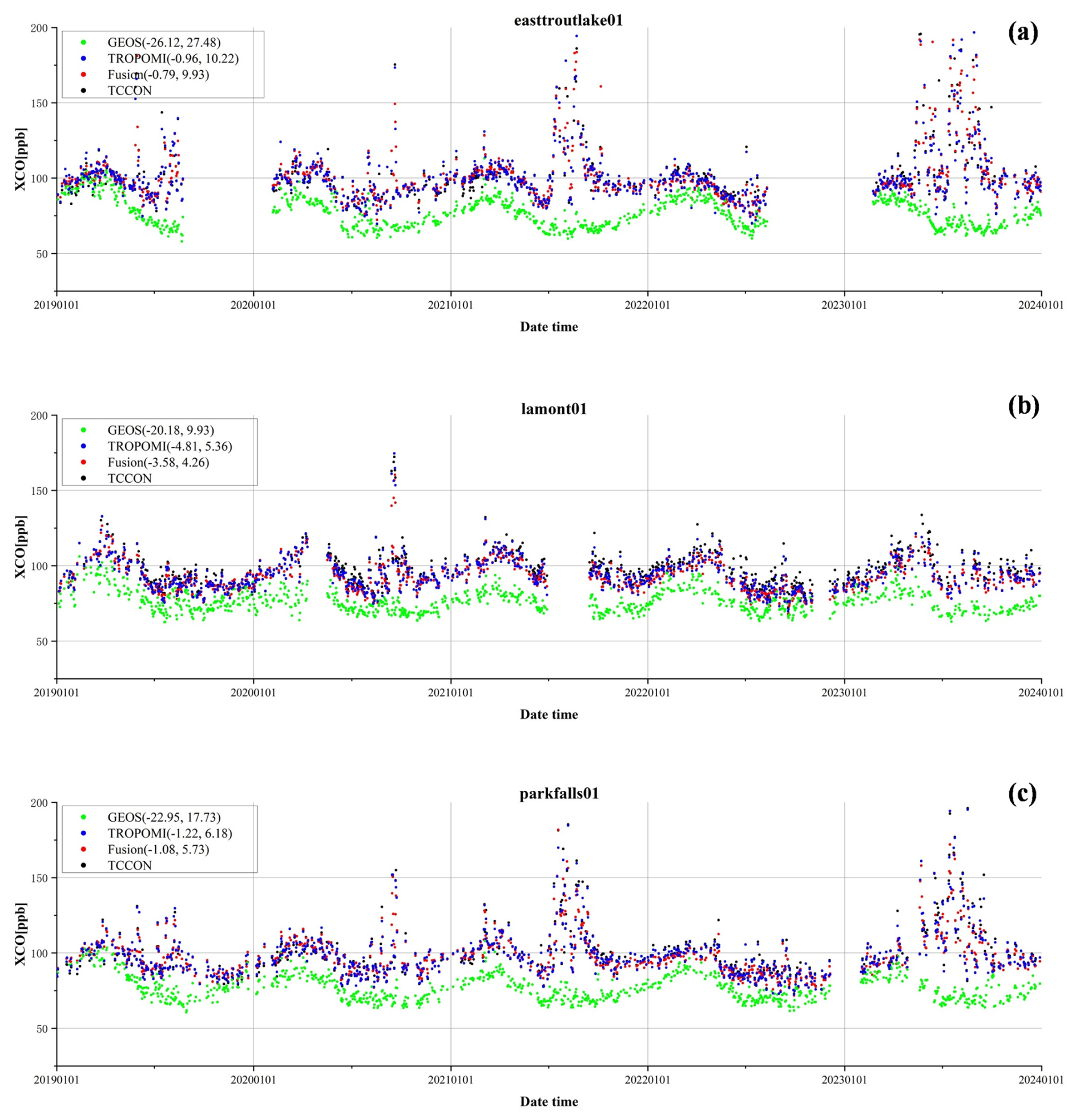
Figure 2 Scatterplots of the time series for daily GEOS-Chem, TROPOMI, fused, and TCCON XCO data at (a) easttroutlake01, (b) lamont01, and (c) parkfalls01. The first and second numbers in parentheses represent μ and σ, respectively. Unit: parts per billion for μ and σ.

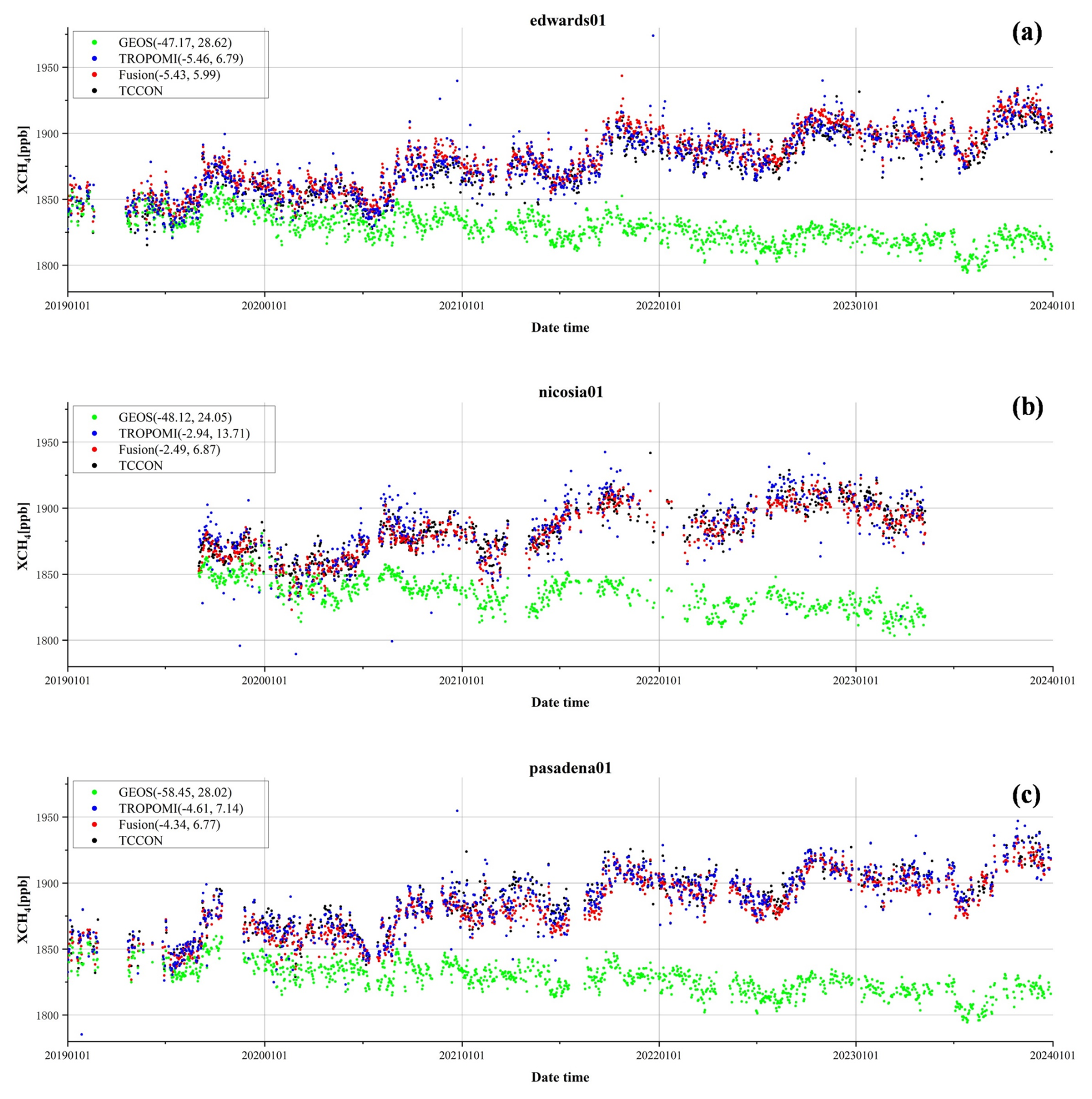
Figure 3 Scatterplots of the time series for daily GEOS-Chem, TROPOMI, fused, and TCCON XCH₄ data at (a) edwards01, (b) nicosia01, and (c) pasadena01. The first and second numbers in parentheses represent μ and σ, respectively. Unit: parts per billion for μ and σ.

GEOS-Chem simulations show a systematic low bias relative to TCCON observations. The raw, uncorrected GEOS-Chem simulations are used as the physical prior in the fusion and reconstruction framework. The mean-bias adjustment is applied only for the diagnostic GEOS-Chem–TCCON comparison and is not used in generating the fused datasets. For each TCCON station and each gas, we calculate the mean difference between GEOS-Chem simulations and TCCON observations over all valid collocated days, and then subtract this mean bias from the GEOS-Chem time series at that station. This procedure removes the station-mean offset while preserving the model's day-to-day variability, allowing a clearer assessment of whether GEOS-Chem captures the temporal variations observed by TCCON. All figures and tables involving this bias-adjusted GEOS-Chem diagnostic comparison are explicitly labeled to indicate that the GEOS-Chem results were bias-corrected before validation.

Following the representative time-series comparison, we further evaluated site-level statistical agreement using scatterplots at selected representative stations under sparse TROPOMI coverage conditions in Figs. 4 and 5. This selection was based on the number of valid collocated samples after applying the missing-rate criterion, rather than on validation performance. Specifically, for each TCCON station, we first applied the qa_value >0.5 quality filter, the 13:30 ± 1 h temporal window, the 2° spatial collocation radius, and the site-day missing-rate criterion (MR >0.5). Subsequently, stations with a relatively large number of valid collocated samples after applying the missing-rate screening criterion were selected for visualization, whereas the overall validation statistics were calculated using all qualified high-missing-rate site-day collocations rather than only these representative stations. For XCO validation, burgos01, izana01, and nicosia01 were selected as representative sites (Fig. 4). At burgos01 and izana01, the fused data show improved agreement with TCCON compared with GEOS-Chem simulations and the original TROPOMI retrievals, as indicated by higher coefficients of determination (R²), lower root-mean-square errors (RMSE), smaller biases (μ), and lower standard deviations (σ). At nicosia01, the fused data do not show a clear improvement over TROPOMI but remain comparable, indicating that the fusion method does not degrade the validation performance at this site. For XCH₄ validation, burgos01, rikubetsu01, and xianghe01 were selected as representative sites (Fig. 5). At burgos01 and xianghe01, the fused data show improved statistical consistency with TCCON relative to GEOS-Chem and modest improvements relative to TROPOMI across several evaluation metrics, including R², RMSE, μ, and σ. At rikubetsu01, the fused data remain comparable to TROPOMI, further indicating the robustness of the fusion method across different sites. Tables S4 and S5 present the validation results for all qualified individual sites for XCO and XCH₄, respectively. Overall, as shown in Tables S4 and S5, the fused data improve at least one of the three reported site-level metrics relative to the original TROPOMI retrievals at 14 of 18 XCO sites (77.8 %) and 10 of 17 XCH₄ sites (58.8 %). Here, improvement refers to higher R², lower RMSE, or smaller $\left|\mathit{\mu }\right|$.

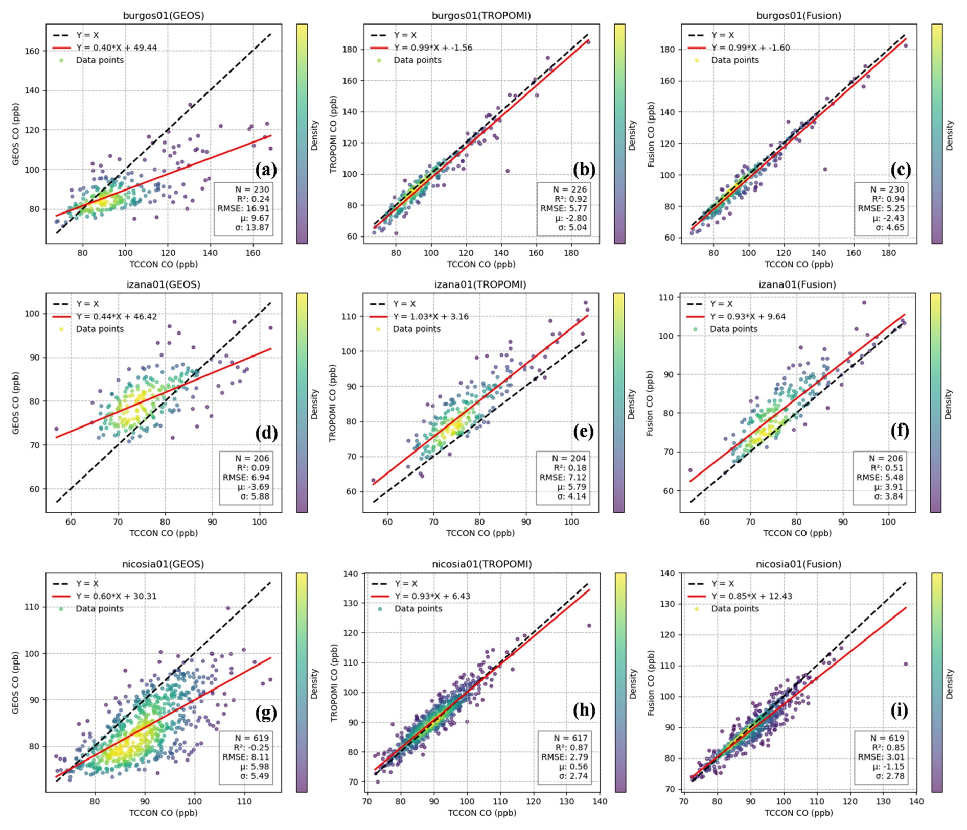
Figure 4 Density scatterplots of the independent validation results for GEOS-Chem, TROPOMI, and fused XCO data at burgos01, izana01, and nicosia01 under sparse TROPOMI coverage conditions (MR >0.5). Panels (a), (d), (g); (b), (e), (h); and (c), (f), (i) correspond to GEOS-Chem, TROPOMI, and fused XCO data, respectively. Black dotted and red solid lines indicate the 1:1 line and fitted regression line, respectively. X: TCCON data; Y: GEOS-Chem, TROPOMI, and fused data. Units: ppb for RMSE, μ, and σ.

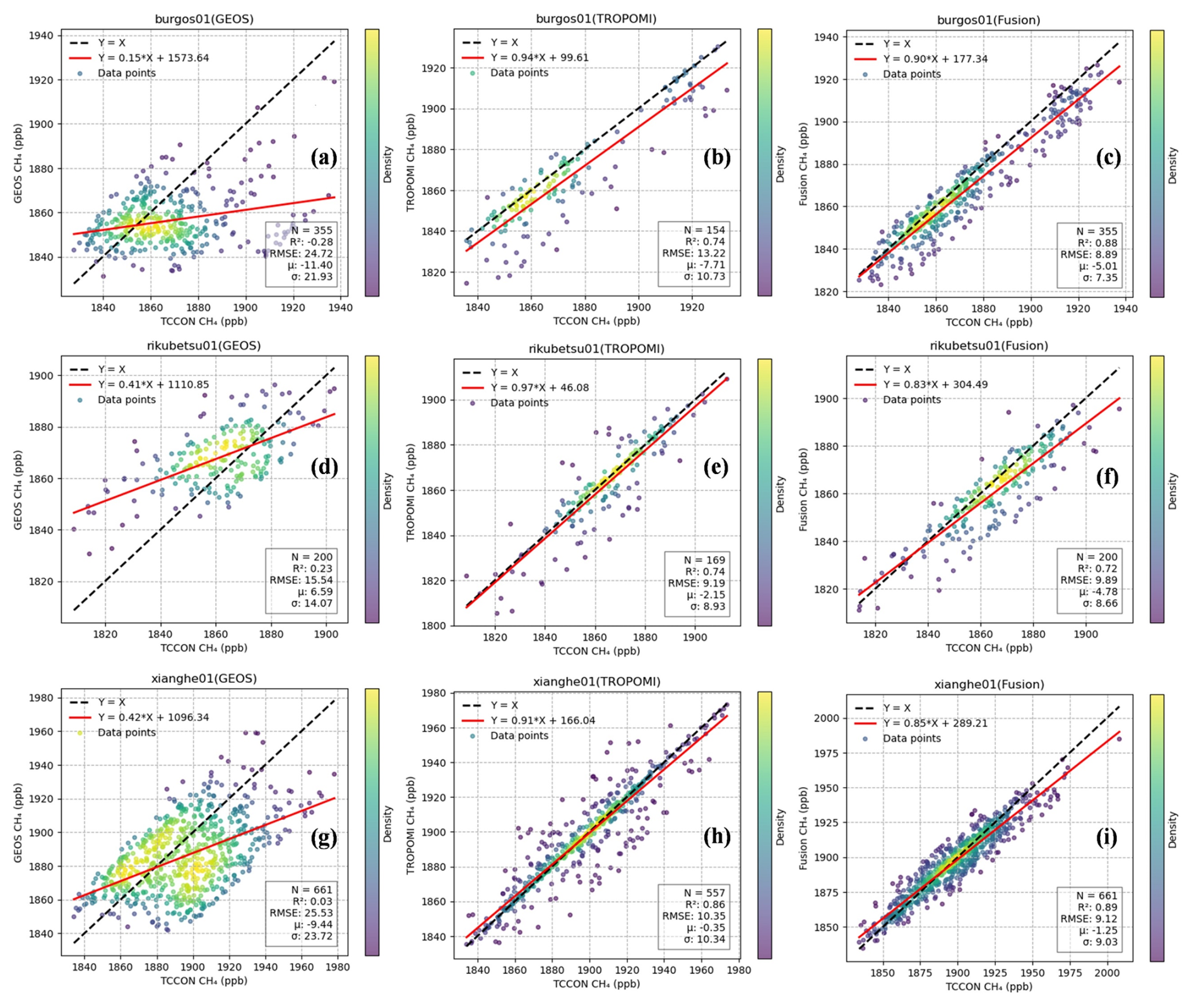
Figure 5 Density scatterplots of the independent validation results for GEOS-Chem, TROPOMI, and fused XCH₄ data at burgos01, rikubetsu01, and xianghe01 under sparse TROPOMI coverage conditions (MR >0.5). Panels (a), (d), (g); (b), (e), (h); and (c), (f), (i) correspond to GEOS-Chem, TROPOMI, and fused XCH₄ data, respectively. Black dotted and red solid lines indicate the 1:1 line and fitted regression line, respectively. X: TCCON data; Y: GEOS-Chem, TROPOMI, and fused data. Units: ppb for RMSE, μ, and σ.

Figure 6 presents the overall validation results for XCO and XCH₄ across all qualified TCCON site-day collocations under sparse TROPOMI coverage conditions (MR >0.5). For XCO, the fused dataset substantially reduces the systematic low bias of GEOS-Chem and shows improved agreement with TCCON compared with the original TROPOMI retrievals across several validation metrics. The fused XCO dataset achieves an R² of 0.91, which is higher than that of TROPOMI, indicating an improved ability to capture the variability observed by TCCON. Its RMSE and standard deviation of the bias are 5.65 and 5.48 ppb, respectively, both lower than those of TROPOMI. The mean bias (μ) is also comparable to that of TROPOMI, suggesting that the fusion process preserves the overall magnitude while reducing random deviations. For XCH₄, the fused dataset also shows improved statistical consistency with TCCON. The fused XCH₄ dataset achieves an R² of 0.83 and a lower standard deviation of the bias than TROPOMI under the same validation protocol. Although its RMSE and mean bias are comparable to those of TROPOMI, the reduced dispersion indicates that the fused dataset provides more stable estimates under sparse-observation conditions. Overall, these results demonstrate that the proposed fusion approach improves the consistency and robustness of XCO and XCH₄ estimates relative to GEOS-Chem and maintains comparable or improved performance relative to TROPOMI, particularly under high-missing-rate conditions.

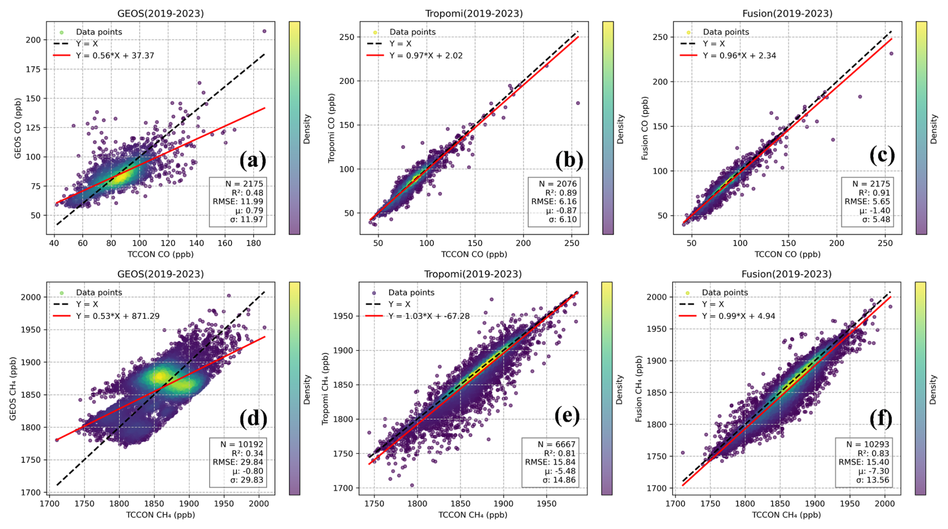
Figure 6 Density scatterplots of the overall validation results for GEOS-Chem, TROPOMI, and fused XCO and XCH₄ data at all corresponding validation sites under sparse TROPOMI coverage conditions (MR >0.5). GEOS-Chem results were bias-corrected before validation. Panels (a), (d); (b), (e); and (c), (f) correspond to GEOS-Chem, TROPOMI, and fused data, respectively. Black dotted and red solid lines indicate the 1:1 line and fitted regression line, respectively. X: TCCON data; Y: GEOS-Chem, TROPOMI, and fused data. Units: ppb for RMSE, μ, and σ.

To demonstrate the performance of our fused datasets under different TROPOMI coverage, we conducted experiments using different MR thresholds. Tables S6 and S7 further quantify how the performance of the fused datasets varies with TROPOMI coverage. For XCO, when the missing rate is low or moderate (MR <0.3 and 0.3≤ MR ≤0.5), TROPOMI shows slightly higher R² values and lower RMSE values than the fused dataset, indicating the high reliability of TROPOMI retrievals under relatively good coverage conditions. However, under sparse TROPOMI coverage conditions (MR >0.5), the performance of TROPOMI decreases, with its R² decreasing to 0.89 and RMSE increasing to 6.16 ppb. In contrast, the fused XCO data maintain a higher R² value of 0.91 and a lower RMSE value of 5.65 ppb, indicating greater robustness under high-missing-rate conditions. For XCH₄, a similar pattern is observed. TROPOMI performs better than the fused product under low and moderate missing-rate conditions, with higher R² and lower RMSE. However, when MR >0.5, TROPOMI performance decreases markedly, with R² declining to 0.81 and RMSE increasing to 15.84 ppb. The fused XCH₄ data show a slightly higher R² of 0.83 and a lower RMSE of 15.40 ppb under the same high-missing-rate condition. Although the fused XCH₄ bias is larger than that of TROPOMI, the higher R² and lower RMSE suggest that the fused dataset reduces overall errors under sparse-observation conditions. Overall, under conditions of good TROPOMI coverage, the fused XCO and XCH₄ datasets perform comparably to the TROPOMI datasets. When TROPOMI retrievals are sparse, the fused datasets show relatively high reliability. These results indicate that our fusion framework is effective for gap-filling applications.

To further position the proposed fused datasets within the current landscape of atmospheric composition products, we compared our TCCON-based validation results with reported accuracies of representative existing products in the literature, rather than conducting a direct pixel-level comparison. Direct product-to-product comparison is not straightforward because existing products differ in target species, input observations, assimilation or fusion methods, spatial and temporal resolutions, and validation protocols. For example, CAMS-EGG4 provides global greenhouse-gas reanalysis fields for CO₂ and CH₄ by combining model and satellite information within the ECMWF Integrated Forecasting System, but it does not provide a TROPOMI-based XCO product directly comparable to the fused XCO dataset developed here (Agustí-Panareda et al., 2023). Agustí-Panareda et al. (2023) reported that CAMS-EGG4 generally shows monthly systematic and random errors for CO₂ and CH₄ within about 1 % during 2003–2020, while also noting caveats related to changes in assimilated observations and fixed underlying emissions. Wang et al. (2023) developed a daily seamless 0.25° global XCO₂ and XCH₄ fusion product from GOSAT, OCO-2, and CAMS-EGG4, and reported TCCON validation statistics of σ≈1.18 ppm for XCO₂ and σ≈11.3 ppb for XCH₄, with R² values of 0.91–0.95 for XCO₂ and 0.90 for XCH₄. In comparison, our fused datasets achieve R² values of 0.91 for XCO and 0.83 for XCH₄ against TCCON. Although these values are not strictly comparable because of differences in target gases, input data, and validation settings, they indicate that the proposed TROPOMI–GEOS-Chem fusion framework provides competitive TCCON-based validation performance while extending daily gap-free mapping to both XCO and XCH₄ at global 0.25° resolution and China-specific 0.05° resolution.

Note that averaging kernels (AKs) were not explicitly applied in the TCCON comparison. This choice was made because the validation focuses on column-averaged dry-air mole fractions after strict quality filtering and spatial–temporal aggregation, for which AK-related smoothing differences are expected to be smaller than retrieval noise, sampling gaps, and spatial representativeness errors. Previous TROPOMI XCH₄/XCO validation studies have shown that AK-related adjustments can be small when column averaging kernels are close to unity in the lower atmosphere (Schneising et al., 2026), although rigorous validation studies still account for smoothing uncertainty and a priori profile effects (Sha et al., 2021). Nevertheless, we acknowledge that ignoring AKs may introduce residual smoothing uncertainty, especially under cloudy conditions or in regions with strong vertical gradients.

3.2 Multi-scale spatiotemporal analysis

Figure S3 illustrates the comparison of worldwide yearly GEOS-Chem, TROPOMI, fused XCO, and XCH₄ for the years 2020 and 2022. The fused data exhibit a similar geographical distribution with TROPOMI. Despite a substantial underestimation of GEOS-Chem, it retains a robust geographic distribution alignment with TROPOMI, providing a critical reference for data fusion, and this underestimation is markedly altered post-fusion.

Figure S4 illustrates the global distribution of fused XCO and XCH₄ for three representative days in 2020 and 2022, respectively. The fusion findings, as seen in the image, offer comprehensive information on atmospheric CO and CH₄, distinctly revealing their worldwide geographical distribution. For comparison, Fig. S5 illustrates the global distribution of XCO and XCH₄ observed by TROPOMI on these corresponding days. Meteorological factors have resulted in several gaps in the satellite observations, particularly evident in the XCH₄ data, when compared to Fig. S3. Figure S3 illustrates that the fused data addresses the deficiencies in geographical and temporal information, so improving data continuity while preserving the integrity of the satellite observations.

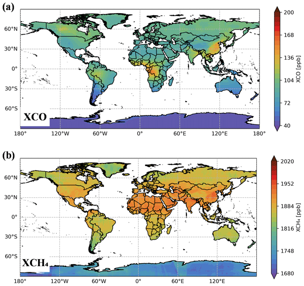
Figure 7 illustrates the global multi-year average distributions of fused XCO and XCH₄ for the period 2019–2023. Elevated concentrations of both gases are predominantly observed across Asia, particularly over China and India. For XCO, distinct high-value regions are also evident in Central Africa and northern South America. Figures S6 and S7 illustrate the seasonal averages of the fused global XCO and XCH₄ data from 2019 to 2023. The seasonal variations in the geographical distribution are distinctly captured by the fusion results. Notably, XCO exhibits more pronounced spatiotemporal variability compared to XCH₄. Specifically, CO tends to be spatially concentrated in certain regions, whereas CH₄ displays a relatively more uniform global distribution.

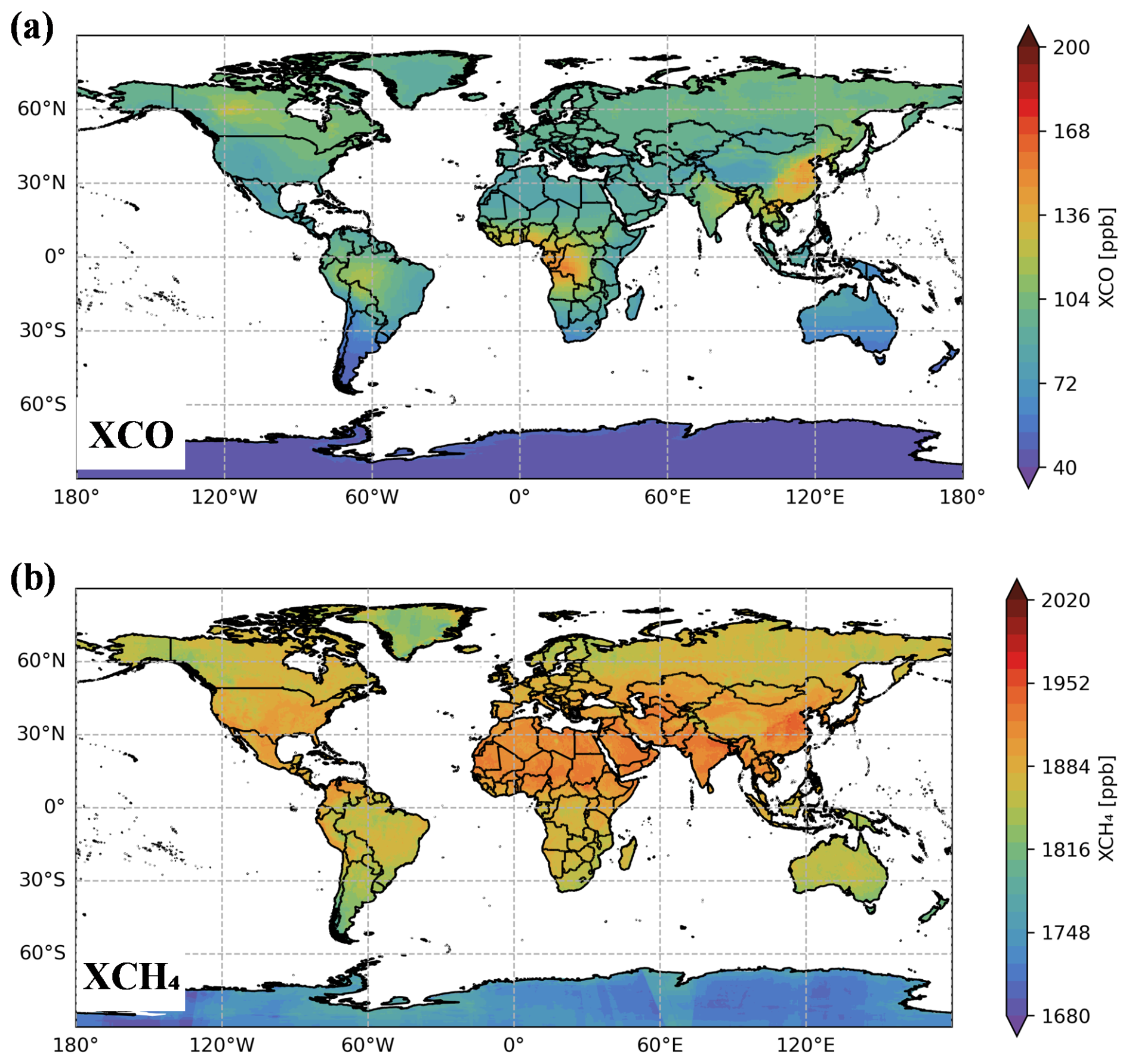
Figure 7 Multi-year mean global concentration distributions of fused (a) XCO and (b) XCH₄ data from 2019 to 2023. Color bars indicate XCO and XCH₄ concentrations in parts per billion.

Figures S8 and S9 illustrate the spatial distribution of the annual rates of change in global XCO and XCH₄ from 2019 to 2023. For each grid cell, the rate of change is estimated by applying ordinary least-squares linear regression to the five annual mean values. Based on this analysis, XCO shows an increasing tendency over North America, whereas Central Africa and Eastern China show decreasing tendencies during 2019–2023 (Fig. S8). For XCH₄, the global annual mean increases over the same period, with a larger positive rate of change observed over Central Africa (Fig. S9).

3.3 Local high-resolution data analysis

To enhance the refinement capability of our fused data, we employed GEOS-Chem to simulate 0.25×0.3125 nested gridded data for the Chinese region. Utilizing the same methodology, we refined the fused data for this region, achieving a grid accuracy of 0.05°, which served as the basis for our analysis of the local area in China.

Figures S10 and S11 illustrate the variations in XCO and XCH₄ from the TROPOMI and fusion datasets during the late August 2022 Chongqing hill fire. To quantify the concentration enhancements, the fire-affected area is defined as a localized domain of 29°–30.5° N and 105.5°–107.5° E, based on the spatial extent of thermal anomalies and smoke plumes observed during the peak of the event. The active fire period is defined as 21–31 August 2022, while 10–20 August 2022 is used as the reference period. The reference period is selected as an adjacent pre-fire baseline, rather than a climatological baseline, to reduce the influence of broader seasonal variability and to better isolate short-term concentration changes associated with the fire episode. Mean XCO and XCH₄ values are calculated by averaging all grid cells within the defined fire-affected domain for each day. The reported enhancements are then calculated as the difference between the mean concentrations during the active fire period and those during the reference period. Based on this definition, the fused data show average increases of 17.1 ppb for XCO and 24.5 ppb for XCH₄ during the fire period. The comparison also indicates that the fused datasets preserve local spatial features observed by TROPOMI while providing more complete spatial coverage over the fire-affected region.

Rice paddies are an important source of CH₄ emissions, while associated agricultural activities, such as crop-residue burning, may also affect regional CO variability. Therefore, we further analyzed the short-term temporal changes in XCO and XCH₄ over the major rice-growing regions of Northeast and Southeast China to evaluate the applicability of the high-resolution fused datasets in agricultural emission-related regions. Figures 8 and 9 show the temporal variations in XCO and XCH₄ derived from TROPOMI and the fused data over these regions, respectively. To reduce the influence of the seasonal cycle, the short-term rates of change were derived using harmonic regression with annual and semiannual terms, and the corresponding 95 % confidence intervals are provided in Tables S9 and S10.

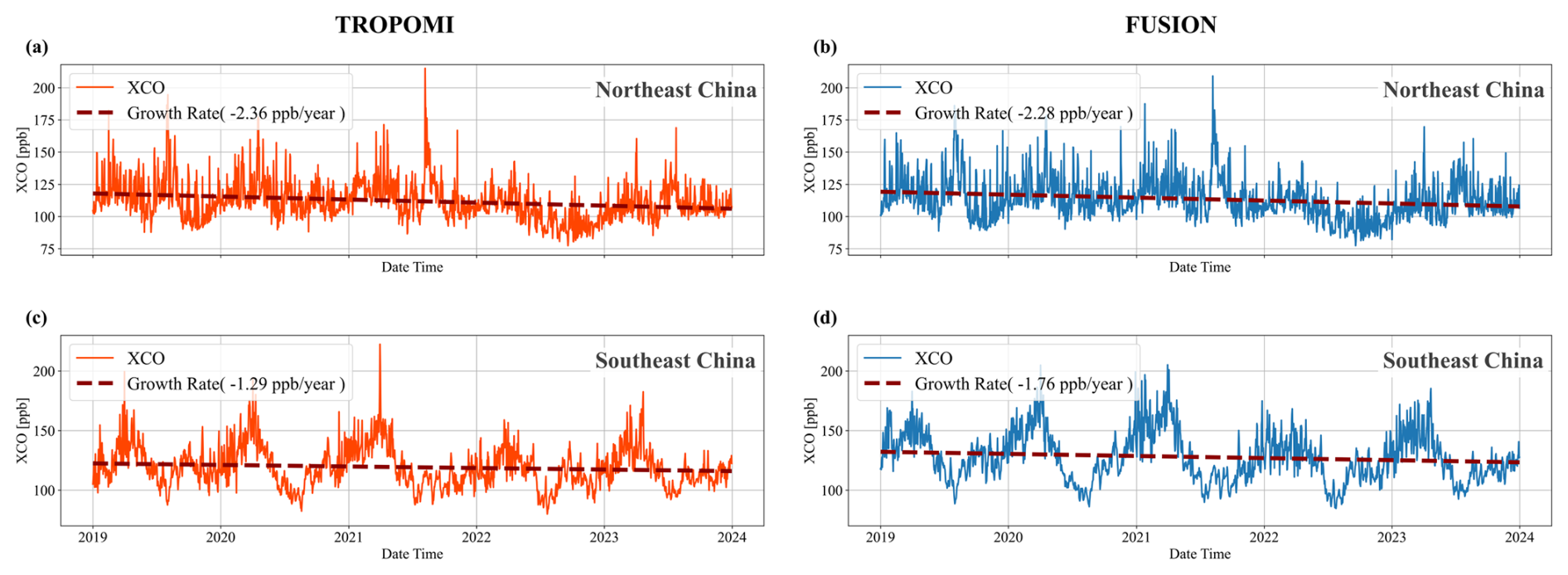
Figure 8 Daily time series of TROPOMI and fused XCO data over rice-growing regions in (a, b) Northeast China and (c, d) Southeast China. Red dashed lines indicate short-term rates of change derived from harmonic regression after accounting for the seasonal cycle, with values shown in parentheses. Unit: parts per billion per year.

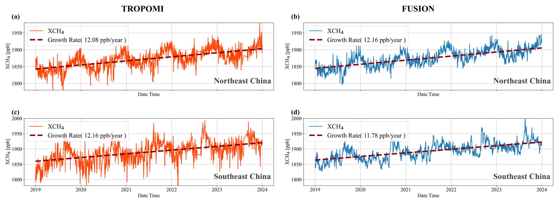
Figure 9 Daily time series of TROPOMI and fused XCH₄ data over rice-growing regions in (a, b) Northeast China and (c, d) Southeast China. Red dashed lines indicate short-term rates of change derived from harmonic regression after accounting for the seasonal cycle, with values shown in parentheses. Unit: parts per billion per year.

The results show that XCO exhibits negative short-term rates of change in both the satellite and fused datasets across the rice cultivation areas of Northeast and Southeast China. In Northeast China, the XCO rate is −2.36 ppb yr⁻¹ for TROPOMI and −2.28 ppb yr⁻¹ for the fused data. In Southeast China, the XCO rate is −1.29 ppb yr⁻¹ for TROPOMI and −1.76 ppb yr⁻¹ for the fused data. The consistent negative rates indicate that the fused dataset preserves the main decreasing XCO signal observed by TROPOMI. Differences between the two datasets may be partly related to the uneven temporal sampling of TROPOMI caused by clouds, aerosols, and retrieval filtering, whereas the fused dataset provides spatially and temporally continuous fields.

In contrast, XCH₄ exhibits positive short-term rates of change in both the satellite and fused datasets. In Northeast China, the XCH₄ rate is 12.08 ppb yr⁻¹ for TROPOMI and 12.16 ppb yr⁻¹ for the fused data. In Southeast China, the XCH₄ rate is 12.16 ppb yr⁻¹ for TROPOMI and 11.78 ppb yr⁻¹ for the fused data. The close agreement between the two datasets indicates that the fused dataset preserves the main increasing XCH₄ signal observed by TROPOMI while providing improved temporal continuity.

3.4 Discussion of uncertainties and limitations

Although the proposed fusion framework substantially improves the spatial continuity of TROPOMI XCO and XCH₄ products and provides daily gap-free fields, several limitations should be considered when using the fused datasets.

Figures 10–11 show the temporal and latitudinal distributions of daily biases between GEOS, Fused, TROPOMI, and TCCON. Overall, GEOS exhibits a clear systematic underestimation of both XCO and XCH₄ relative to TCCON, especially after 2020, when strong negative biases appear at many sites. After fused, the biases are substantially reduced, with colors generally shifting from dark blue to light blue or near white. This indicates that the fusion method effectively corrects the systematic underestimation in GEOS and improves its consistency with TCCON. Compared with GEOS, TROPOMI shows smaller overall biases, but it has more missing data and still exhibits localized positive or negative biases at some sites and periods. Overall, the fusion product performs better than GEOS in reducing biases and improving reliability, although residual uncertainties remain at individual sites.

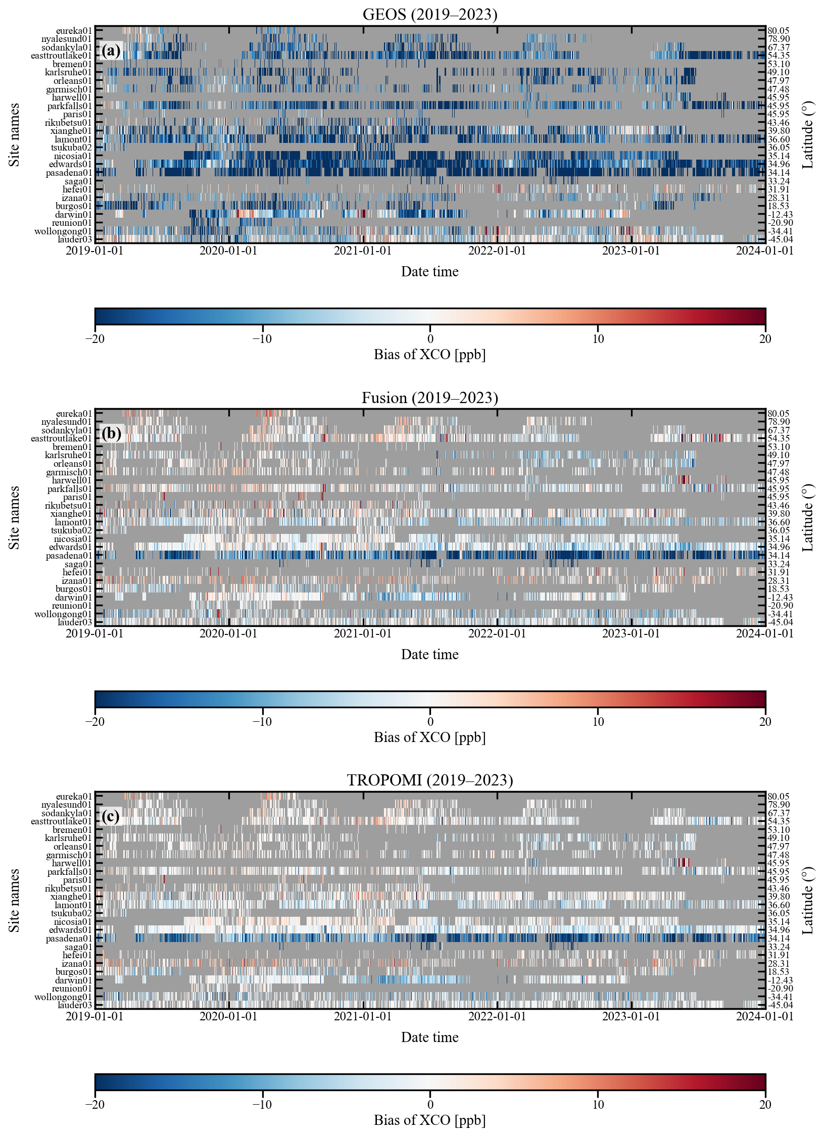
Figure 10 Heat maps of the biases between daily (a) GEOS, (b) fused, and (c) TROPOMI XCO and TCCON XCO over time and latitude. Color ramps stand for the biases of XCO. Background colors (grey) indicate the missing data.

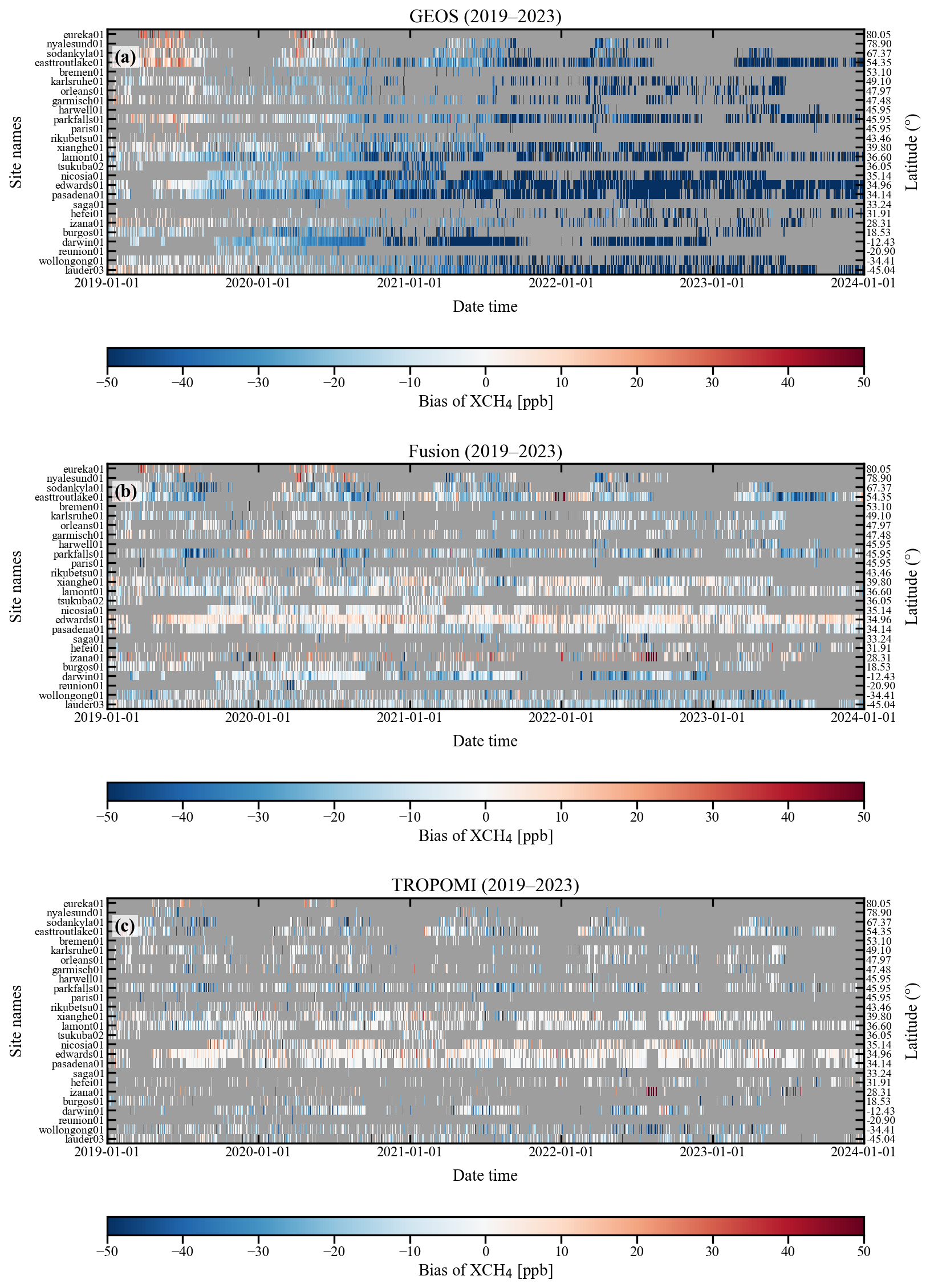
Figure 11 Heat maps of the biases between daily (a) GEOS, (b) fused, and (c) TROPOMI XCH₄ and TCCON XCH₄ over time and latitude. Color ramps stand for the biases of XCH₄. Background colors (grey) indicate the missing data.

AKs are an important source of uncertainty in comparisons between satellite retrievals and model simulations because they describe the vertical sensitivity of TROPOMI retrievals. To evaluate this effect, we conducted an AK sensitivity test using the 2019 CO data by comparing GEOS-Chem XCO with TROPOMI XCO before and after applying the TROPOMI CO column averaging kernels. As shown in Table S11, applying the TROPOMI CO column averaging kernels slightly increased the R² from 0.543 to 0.565, while the RMSE increased from 28.17 to 28.66 ppb and the mean bias changed from −17.09 to −18.34 ppb. These results indicate that AK treatment has a limited influence on the column-concentration-based fusion results in this experiment.

Another concern relates to the dependence of the fused datasets on the accuracy of the GEOS-Chem prior and the representativeness of valid TROPOMI observations. GEOS-Chem provides physically consistent large-scale background information, but it carries uncertainties from emission inventories, transport, chemistry, boundary conditions, vertical mixing, and other model parameterizations. In regions or periods where valid TROPOMI retrievals are persistently sparse – such as the Intertropical Convergence Zone, high-latitude zones, or heavily polluted areas with dense cloud or aerosol cover – the reconstruction relies more strongly on the GEOS-Chem prior and the DCT/SVD spatiotemporal structure. Consequently, systematic biases in the prior model may propagate into the fused fields. Users are therefore advised to consult the obs_mask variable provided in the dataset to assess observational support and to interpret the reconstructed values cautiously in persistently missing regions.

Figure S12 shows that the fused XCO data generated directly at the native 2° × 2.5° resolution (Fig. S12a) and the 0.25° fused XCO data aggregated to the same 2° × 2.5° grid (Fig. S12b) present relatively similar global spatial distributions, with relatively high XCO over East Asia, central Africa, and parts of South America. The quantitative comparison results in Fig. S13 also show high consistency, with R²=0.926, RMSE =6.93 ppb, and mean bias =0.15 ppb. These results indicate that the 0.25° fused XCO data preserve the coarse-scale spatial structure, and that the resolution mismatch does not have a substantial influence on the coarse-scale reconstruction fidelity of XCO.

The masked residual-learning strategy itself introduces uncertainty in persistently missing regions. Because the residual U-Net is trained only at valid TROPOMI pixels, the model learns the statistical relationship between the preliminary reconstruction error and the input predictors under observed conditions. When applied to unobserved regions – especially those with persistent cloud cover or aerosol contamination – the model infers the most likely residual pattern given similar meteorological and spatiotemporal conditions, rather than the exact unobserved atmospheric state on a specific day. This does not invalidate the gap-filling framework, but it implies that reconstructed values in long-term data gaps should be understood as observation-constrained estimates rather than direct measurements. Users should be aware of this extrapolation uncertainty when analyzing local short-lived anomalies in persistently cloudy regions.

Finally, possible discontinuities associated with changes in the input satellite product should be considered. The TROPOMI pixel size changed around June 2019 from 7.0 km × 7.0 km to 7.0 km × 5.5 km, which may affect sampling density and local spatial representativeness. Although the fusion framework uses gridding, quality filtering, and residual correction to mitigate such effects, subtle artifacts or temporal discontinuities may remain. Caution is advised when interpreting local-scale or short-term variations that span this instrumental transition.

In summary, the fused datasets are most suitable for studying daily to seasonal spatiotemporal variability, improving data continuity and spatial coverage, examining regional-scale events (e.g., biomass burning emissions), and supporting comparative analyses during 2019–2023. For fine-scale local anomaly detection in persistently missing regions, for applications in areas lacking independent ground-based validation, or for studies requiring strict profile-sensitive validation or long-term climate trend attribution, users should consult the observation-support variables, including obs_mask, MR, and observation_fraction, and carefully consider all the limitations discussed above.

4 Fused dataset summary

The final data products generated in this study consist of daily gap-free fused XCO and XCH₄ datasets for the period 2019–2023. Two spatial scales are provided. The global product contains daily XCO and XCH₄ fields at 0.25° × 0.25° resolution, covering the global domain. The regional product provides higher-resolution daily XCO and XCH₄ fields over China at 0.05° × 0.05° resolution. Both products are reported as column-averaged dry-air mole fractions in parts per billion (ppb).

The datasets are distributed in NetCDF4 (.nc/.nc4) format. Each monthly file contains gridded daily fields with the dimensions “time”, “lat”, and “lon”. The “time” coordinate is defined using CF-style physical time units, for example, “days since 2019-01-01 00:00:00”, with “time = 0” corresponding to the first day of the month. Users can therefore retrieve a specific daily field by selecting the corresponding “time” index in the monthly NetCDF file. The coordinate variables “lat” and “lon” define the spatial grid of each product.

The main data variables are “XCO” and “XCH₄”, representing the fused column-averaged dry-air mole fractions of CO and CH₄, respectively. In addition, an obs_mask variable is provided to indicate whether the value at each grid cell is a TROPOMI observation or reconstructed by the fusion framework. The obs_mask variable is a dimensionless binary mask, where obs_mask = 1 indicates that the value at that grid cell and day is a TROPOMI observation, while obs_mask = 0 indicates that the value was generated by the proposed reconstruction method.

An “observation_fraction” variable is also included in each monthly file. This variable is calculated as the mean of “obs_mask” over the “time” dimension and represents the fraction of days in that month for which valid TROPOMI observations are available at each grid cell. For example, “observation_fraction = 1” indicates that valid satellite observations are available for all days in the month at that grid cell, whereas “observation_fraction = 0” indicates that all daily values at that grid cell are reconstructed by the fusion framework. This information is provided to prevent users from interpreting the entire gap-free product as purely observation-based.

Because of file-size and repository upload limitations, the daily data are organized into monthly NetCDF files rather than being provided as a single file for the entire study period. This monthly organization does not indicate temporal averaging. Each monthly file contains all daily fields for that calendar month.

The revised NetCDF files include CF-style metadata, including coordinate attributes, variable long names, units, missing-value definitions, temporal coverage, spatial resolution, product region, data source, author, institution, and contact information. The main variables included in the released NetCDF files are summarized as follows: “XCO” (ppb), fused column-averaged dry-air mole fraction of carbon monoxide; “XCH₄” (ppb), fused column-averaged dry-air mole fraction of methane; “obs_mask” (unitless binary mask), indicating whether the grid-cell value is derived from a valid satellite observation (“1”) or reconstructed by the proposed fusion method (“0”); “observation_fraction” (unitless fraction from 0 to 1), indicating the monthly fraction of days with valid satellite observations at each grid cell; “time”, the daily time coordinate within each monthly file, defined using CF-style units; and “lat” and “lon”, the latitude and longitude coordinates of the gridded product.

5 Data availability

The global (0.25°) and China-specific (0.05°) daily gap-free XCO and XCH₄ datasets (2019–2023) generated in this study are openly available in the Zenodo repository at https://doi.org/10.5281/zenodo.22010891 (An et al., 2026).

6 Conclusions

This study developed a two-stage signal-domain guided spatio-temporal fusion framework for generating continuous XCO and XCH₄ products by integrating GEOS-Chem simulations with TROPOMI satellite observations. The framework first applies 3D DCT and SVD to reconstruct low-rank signal-domain structures, thereby providing a robust prior for missing-value approximation. A lightweight residual convolutional neural network is then used to refine pixel-level residuals under observational constraints. Using this framework, we generated daily continuous XCO and XCH₄ products for 2019–2023 at 0.25° global resolution and 0.05° resolution over China.

Validation against independent TCCON observations shows that the fused datasets improve spatiotemporal continuity while still maintaining good consistency with TCCON data. In the time-series comparison analysis at representative sites, the fused XCO and XCH₄ products generally conform to the temporal variation patterns observed by TCCON and TROPOMI, while reducing the systematic underestimation phenomenon associated with GEOS-Chem simulations. To further evaluate the performance under different TROPOMI data coverage rates, we conducted experiments based on missing-rate thresholds, with three MR intervals: MR <0.3, 0.3≤ MR ≤0.5, and MR >0.5. The results show that when MR <0.3 and 0.3≤ MR ≤0.5, the fused products perform comparably to the original TROPOMI retrievals; whereas under sparse TROPOMI data coverage conditions (MR >0.5), the fused XCO product obtained a higher R² value and a lower RMSE value than the TROPOMI product, with R²=0.91 and RMSE =5.65 ppb. The fused XCH₄ product obtained a higher R² value and a lower RMSE value, with R²=0.83 and RMSE =15.40 ppb. Compared with GEOS-Chem simulations, the fused products significantly reduced systematic bias.

The fused datasets also captured meaningful spatial and temporal patterns of atmospheric CO and CH₄. During 2019–2023, the reconstructed products revealed regional XCO increases in parts of North America, decreases over eastern China, and widespread XCH₄ growth. The high-resolution China product further resolved regional-scale features, including enhanced XCO and XCH₄ during the 2022 Chongqing wildfire event. Over rice-growing regions, the fused datasets preserved the main short-term temporal signals observed by TROPOMI while reducing the influence of uneven sampling caused by satellite data gaps.

By combining the spatiotemporal continuity of GEOS-Chem, the observational constraints of TROPOMI, and signal-domain reconstruction, the fused datasets provide more complete and statistically consistent representations of global and regional XCO and XCH₄ variations. The fusion process also mitigates the systematic underestimation observed in GEOS-Chem simulations. Such model biases may arise from multiple sources, including uncertainties in emission inventories, chemical mechanisms, atmospheric transport, boundary conditions, vertical mixing, and other model parameterizations. Therefore, the fused products can serve as an improved basis for analyzing long-term spatial patterns, seasonal variability, and regional changes in atmospheric CO and CH₄.

Despite these advances, several limitations remain. The fusion framework depends partly on the quality of GEOS-Chem simulations, and residual uncertainties may persist due to imperfect emission inventories, transport representation, chemical mechanisms, and parameterizations. Future work should further improve the prior model fields, refine the fusion strategy, and incorporate additional independent observations, such as GOSAT/GOSAT-2 for CH₄, MOPITT or IASI for CO, and expanded ground-based measurements, to further enhance the robustness and applicability of the dataset. Overall, this study provides continuous, high-resolution, and validated datasets of XCO and XCH₄ that can support future research on atmospheric composition, air quality, emission monitoring, and climate-related applications.