Hydrographic CTD profiles capturing the onset of near-surface stratification in Southwest Greenland fjords during two consecutive spring 2025 field campaigns

In situ hydrographic observations in Greenland fjords remain sparse, particularly during late winter and early spring, despite their importance for Arctic freshwater export, glacier–ocean interactions, and the seasonal development of stratification. A major limitation of many existing hydrographic datasets is the poor representation of the near-surface layer, where meltwater lenses, sharp salinity gradients, and strong density gradients are often concentrated within the upper few metres.

Here we present a quality-controlled conductivity, temperature, and depth dataset comprising 73 vertical hydrographic profiles collected across Southwest Greenland fjords (60.2–69.5° N, 43.6–53.9° W) during two expeditions aboard the icebreaker Le Commandant Charcot: the Sea Ice Measurements for Satellite thickness retrieval Validation campaign (32 profiles, 24 March–4 April 2025) and the Freshwater fluxes and Atlantic-Nordic Seas hydrography campaign (41 profiles, 18–28 April 2025).

The dataset includes pressure, temperature, conductivity, practical salinity, and derived thermodynamic variables. Two RBR Concerto3 conductivity, temperature, and depth instruments sampling at 16 Hz and 2 Hz were processed through a reproducible eight-step workflow including atmospheric-pressure correction, automatic soak detection, signal conditioning, loop removal, thermodynamic calculations, and automated quality control following international ocean-data recommendations.

Unlike many standard conductivity, temperature, and depth products, the processing strategy retains the shallowest valid observations and preserves the native vertical sampling. This enables users to examine thin freshwater lenses and sharp near-surface gradients without systematically excluding the upper few metres of the water column. It also allows alternative vertical averaging or filtering strategies to be applied according to the objectives of future analyses.

Thermohaline diagnostics identify four main hydrographic regimes: coastal and glacier meltwater-influenced waters, Polar Water, Winter Water, and modified Atlantic or Irminger Water. Comparison of the late-winter and early-spring campaigns documents the onset of surface restratification across Southwest Greenland fjords. The strongest freshening and shallow stratification occur in fjords directly influenced by tidewater glaciers, whereas deeper water masses remain comparatively stable over the one-month period.

The dataset is distributed in NetCDF-4 format compliant with Climate and Forecast Metadata Conventions version 1.8 and Attribute Convention for Data Discovery version 1.3, and is publicly available through Zenodo. The processing code is archived on GitHub and Zenodo (https://doi.org/10.5281/zenodo.20489479, Hoareau et al., 2026). Together, these observations provide a valuable resource for studies of Arctic freshwater dynamics, glacier–ocean interactions, and fjord stratification, as well as for ocean model evaluation and satellite product validation.

1 Introduction

Greenland fjords are highly dynamic coastal environments where oceanic waters interact with freshwater inputs from glaciers, runoff, and sea-ice processes. These systems strongly influence regional stratification, circulation, and biogeochemical exchanges, while acting as key gateways linking the Greenland Ice Sheet with the surrounding ocean.

In situ hydrographic measurements within Greenland fjords remain sparse compared to adjacent open-ocean regions. Observations are limited by logistical constraints, seasonal accessibility, and complex fjord geometries. Profiling floats such as Argo cannot operate in these shallow and confined environments, and ship-based surveys are difficult to carry out, particularly under ice-covered conditions. As a result, existing datasets often exhibit uneven spatial and temporal coverage, complicating cross-study comparisons and limiting their use for model evaluation.

A further limitation of many hydrographic datasets is the poor representation of the uppermost metres of the water column. Standard ship-based CTD casts often exclude the near-surface layer because of sensor equilibration or ship disturbance, while Argo floats do not sample shallow, narrow, and ice-affected fjord environments. However, in glacier-influenced fjords, some of the most dynamic hydrographic signals occur precisely in this shallow layer, where meltwater lenses, sharp haloclines, and density inversions can be confined to the upper few metres. Preserving these measurements, together with their quality-control flags, is therefore essential for documenting meltwater-driven stratification that would otherwise be missed or filtered out.

Observations are specially sparse during late winter and early spring. Ship access to fjords is typically restricted by sea-ice cover from November to March, making winter CTD profiles rare (Straneo et al., 2019; Straneo and Cenedese, 2015). Most available datasets are collected during summer and early autumn, when glacier melt and surface runoff are at their peak (Bendtsen et al., 2015; Mortensen et al., 2013; Stuart-Lee et al., 2021). Consequently the winter thermohaline state of Southwest Greenland fjords remains poorly characterised (Straneo et al., 2019). Late-winter profiles capture the hydrographic conditions at the end of the convective season, prior to the onset of freshwater-driven restratification, and provide essential initial conditions for the seasonal evolution of stratification, heat content, and biological productivity (Carroll et al., 2017; Meire et al., 2016; Massicotte et al., 2020).

The SIMSVAL expedition (March–April 2025), conducted aboard the icebreaker Le Commandant Charcot, exploited the vessel's ice-capable operations to access Southwest Greenland fjords during this undersampled late-winter period, yielding 32 CTD profiles. To our knowledge, no published quality-controlled, open-access hydrographic dataset documents the interior of these fjords during late winter. The FANS expedition (April 2025) provides complementary observations during early spring across eight Southwest Greenland fjords. The campaign targeted the hydrographic structure of fjords with contrasting glacier influence, including tidewater glacier fjords, land-terminating systems, and fjords without direct glacier input. Freshwater export from Greenland fjords and the intrusion of Atlantic-origin waters (Atlantic Water and Irminger Water) play a key role in controlling stratification and submarine melting processes (Straneo and Cenedese, 2015; Rignot et al., 2015; Jenkins, 2011). The April sampling captures the onset of the spring thermohaline transition, when surface restratification begins under the combined influence of meltwater input and atmospheric forcing (Stuart-Lee et al., 2021; Meire et al., 2016; Jackson et al., 2014).

Standardized and well-documented hydrographic datasets are essential for improving the characterisation of Arctic coastal systems. Datasets produced through consistent workflows and quality-control procedures provide a robust basis for analysing water-mass structure, vertical stratification, freshwater influences, and for validating models and satellite products.

Here we present the quality-controlled CTD dataset from the SIMSVAL and FANS campaigns conducted in March–April 2025. The dataset comprises 73 profiles from Southwest Greenland fjords (60.2–69.5° N), covering the late-winter to early-spring period across fjords with different glacier influence. All profiles were processed through a common reproducible pipeline and quality-controlled following QARTOD, Argo, and SeaDataNet standards. Beyond providing an open hydrographic data product, the dataset documents the onset of near-surface stratification and its modulation by glacier influence. A key feature of the dataset is the retention of valid near-surface measurements, which supports the analysis of fine-scale upper-ocean stratification. In addition, the original high vertical resolution of the profiles has been preserved, enabling users to adapt the vertical binning and resolution according to the needs of future analyses.

This paper describes the dataset, its processing pipeline, and its technical validation. Section 2 presents the study region and field campaigns. Section 3 describes the instrumentation. Section 4 details data processing and quality control. Section 5 describes the dataset structure and file format. Section 6 presents the technical validation and a scientific characterisation of the water column, including the March–April thermohaline transition.

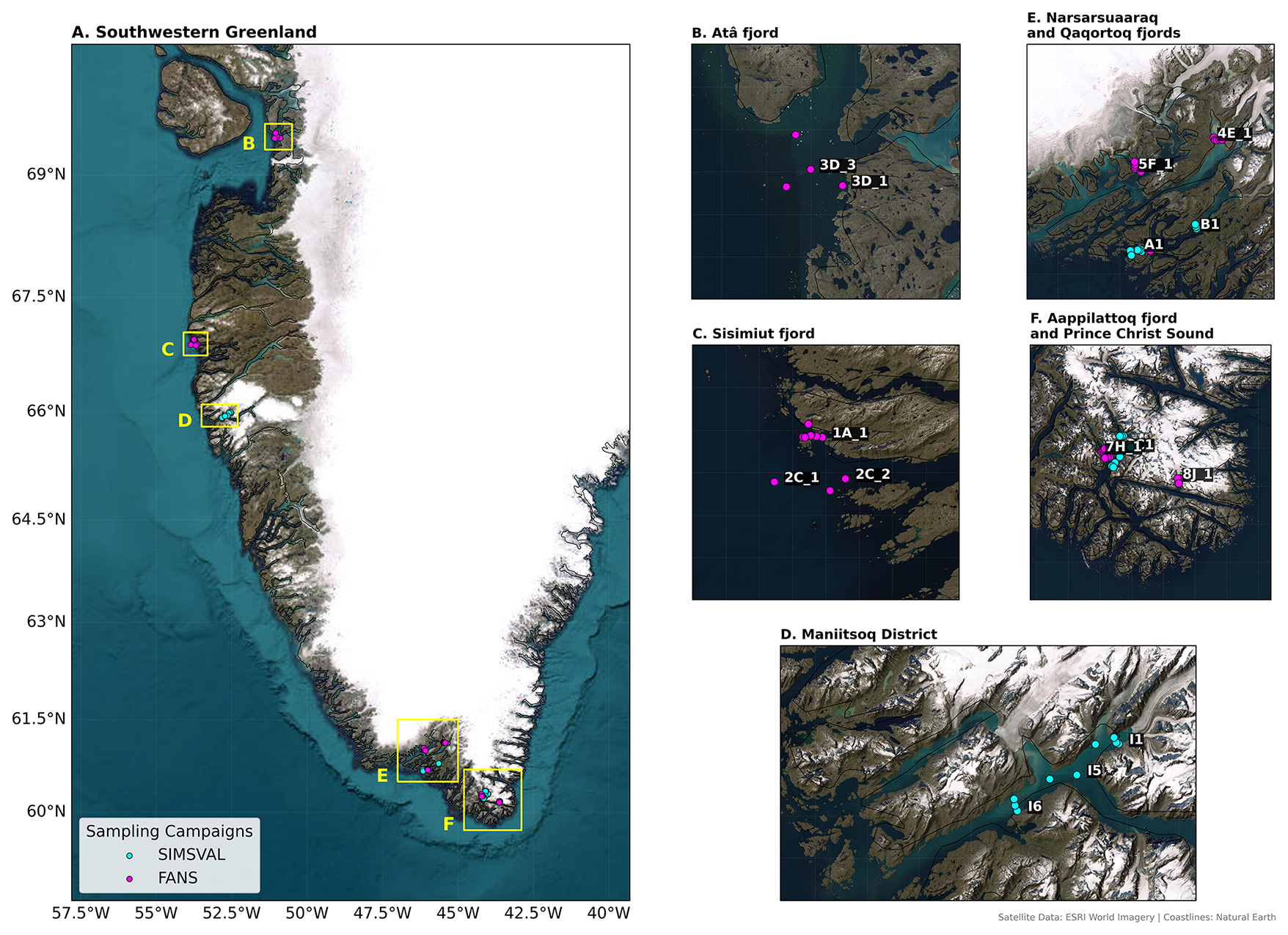
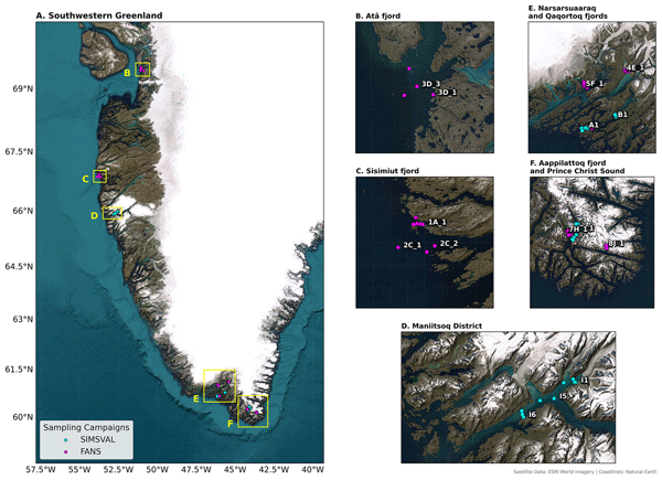
Figure 1 Study region and CTD station distribution along the south-west coast of Greenland during the SIMSVAL and FANS 2025 campaigns. Panel (A) shows the regional overview, with yellow boxes indicating the locations of the detailed subregions displayed in Panels (B)–(F): (B) Atâ fjord, (C) Sisimut fjord, (D) Maniitsoq district, (E) Narsarsuaaraq and Qaqortoq fjords, and (F) Aappilattoq and Prince Christian Sound. Cyan circles correspond to SIMSVAL stations collected between 21 March and 5 April 2025 (n=32), while magenta circles indicate FANS stations collected between 18 and 28 April 2025 (n=41). Station labels correspond to the identifiers used in the dataset files and metadata tables. Satellite imagery background from ESRI World Imagery|Powered by Esri; coastlines in black from Natural Earth.

2 Study region and field campaigns

2.1 Study region

This dataset covers fjord and coastal environments along the Southwest Greenland margin between 60.2 and 69.5° N and (43.6–53.9° W), and spans contrasting fjord environments from the Narsarsuaq–Prince Christian region near Cape Farewell (∼60° N) to the Disko Bay approaches at Atâ Sund (∼69° N; Fig. 1). The sampled areas include fjords connected to active tidewater glaciers, semi-enclosed sill fjords, and more open coastal systems influenced by shelf circulation. Together, these regions constitute one of the most dynamic and rapidly changing coastal environments of the sub-Arctic North Atlantic.

West Greenland fjords are glacially carved systems, typically 2–20 km wide and 20–150 km long, with basin depths reaching 200–1300 m. Sill depths at fjord mouths range from tens of metres (e.g. Tunuillarfik near Narsarsuaq) to more than 200 m in the Nuuk–Godthåbsfjord system (Mortensen et al., 2013), and exert a primary control on the exchange of water masses between fjord interiors and the adjacent continental shelf (Mortensen et al., 2014). Many fjords terminate in active tidewater glaciers or marine-terminating fronts that deliver freshwater to the fjord water column as liquid subglacial discharge, surface runoff, and calving icebergs (Cowton et al., 2015; Mankoff et al., 2016).

The hydrographic structure of the Southwest Greenland shelf and fjord systems is governed by the West Greenland Current (WGC), which transports contrasting Arctic- and Atlantic-origin water masses poleward along the continental margin (Straneo and Cenedese, 2015; Rysgaard et al., 2020). Following the updated classification proposed by Rysgaard et al. (2020), the regional water column is characterised by the interaction between Polar Water (PW), coastal and glacier meltwater-influenced surface waters (CW/GMW), Winter Water (WW), and Atlantic-origin Irminger Water (IW/WGIW).

At depth, warm and saline Irminger Water (IW or WGIW) constitutes the main subsurface heat reservoir of SouthWest Greenland fjords and the primary oceanic heat source for submarine melting at tidewater glacier fronts (Holland et al., 2008; Jenkins, 2011). This water mass is characterised by relatively high salinity and positive temperature (S_A≳33.3 g kg⁻¹, Θ>0 °C in the present dataset) and intrudes into fjord basins deeper than the local sill. Irminger Water is a regional branch of Atlantic Water (AW): after crossing the Iceland–Faroe Ridge, North Atlantic Water circulates cyclonically through the Irminger Sea and rounds Cape Farewell before feeding the WGC along the West Greenland shelf (Straneo and Heimbach, 2013; Daniault et al., 2016). Along this pathway, the water mass is modified through mixing and cooling, becoming slightly fresher and colder than the Atlantic Water entering the Arctic through Fram Strait, while remaining thermodynamically distinct from ambient fjord waters.

In the upper water column, relatively cold and fresh Polar Water (PW), partly derived from Arctic-origin waters transported southward by the East Greenland Current and recirculated around Cape Farewell, occupies the outer shelf and fjord surface layers (Rysgaard et al., 2020). Within glacier-influenced fjords, local freshwater inputs from runoff, iceberg melt, and subglacial discharge generate buoyant coastal and glacier meltwater-influenced waters (CW/GMW), frequently confined to the upper few metres during spring. Between these surface waters and the Atlantic-origin subsurface layer, Winter Water (WW) forms a temperature minimum layer associated with winter cooling and convective mixing. The interaction and mixing between PW, CW/GMW, WW, and IW/WGIW produce the characteristic stratified thermohaline structure of Southwest Greenland fjords documented in this study.

Seasonal variability strongly modulates the hydrographic structure of Southwest Greenland fjords. Sea-ice cover, which typically persists in northern fjords from November to April or May, acts both as an observational barrier and as a surface buoyancy forcing that suppresses deep convection and controls the timing of spring restratification (Straneo et al., 2019). Following ice break-up, increasing meltwater input from sea ice, runoff, and subglacial discharge drives rapid near-surface freshening and the development of shallow stratified surface layers. By summer, surface salinities in glacier-influenced inner fjords can fall below 28 PSU (Stuart-Lee et al., 2021; Mortensen et al., 2013).

These seasonal changes strongly influence fjord–shelf exchange, upper-ocean stratification, heat delivery toward glacier fronts, and the timing of the spring phytoplankton bloom (Meire et al., 2016; Carroll et al., 2017; De Andrés et al., 2020). However, observations during the late-winter to early-spring transition remain scarce because fjord access is frequently limited by sea ice and harsh weather conditions. This poorly sampled period corresponds precisely to the onset of the surface restratification documented in the present dataset.

2.2 SIMSVAL expedition leg (March–April 2025)

The SIMSVAL expedition (Sea Ice Measurements for Satellite thickness retrieval VALidation; cruise CC210325) was conducted aboard Le Commandant Charcot from 21 March to 5 April 2025, departing from Reykjavík (Iceland) and concluding in Nuuk (Greenland). The primary scientific objective of the campaign was the characterization of sea ice properties using an L-band radiometer and the SIMS (Sea Ice Monitoring System) instrument for satellite sea-ice thickness validation. The collection of oceanographic CTD profiles constituted a secondary objective, aimed at documenting ice–ocean interactions in glacier-fjord systems along the vessel track.

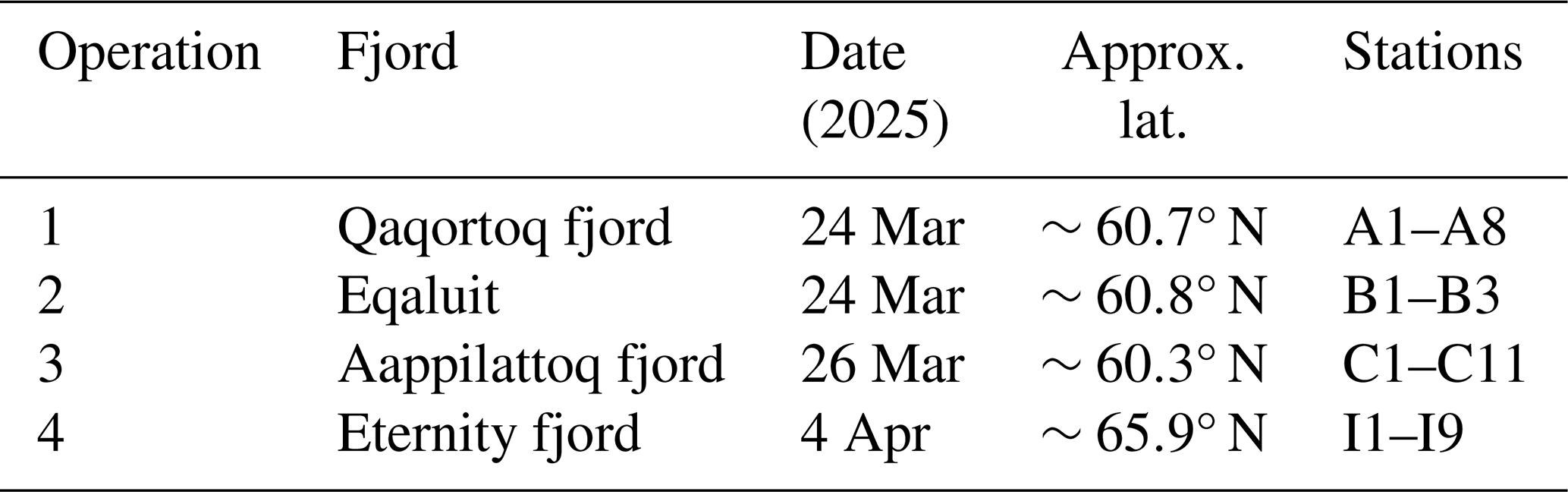
Hydrographic profiles were carried out from a zodiac yielding 32 ocean profiles distributed across four fjord systems in Southwest Greenland (60.2–66.0° N, 44–53° W; Table 1): Qaqortoq fjord (group A, 60.7° N, 46.1° W), Eqaluit (group B, 60.8° N, 45.6° W), Aappilattoq fjord (group C, 60.3° N, 44.1° W), and Eternity fjord in the Nuuk approaches (group I, 65.9° N, 52.7° W). A second CTD instrument (owned by the vessel company) was co-deployed at one station. That instrument was a RBR Concerto3 CTD and acquired at 2 Hz CTD (hereafter referred to as B1_val, within 2 min of station B1) to provide a direct inter-sensor comparison under quasi-identical ocean conditions.

Table 1 SIMSVAL zodiac CTD operations (cruise CC210325, March–April 2025). Station groups follow the identifier scheme used throughout this paper.

2.3 FANS expedition leg (April–May 2025)

The FANS expedition (Freshwater fluxes and Atlantic-Nordic Seas hydrography; cruise CC170425) was conducted from 17 April to 2 May 2025, departing from Nuuk (Greenland) and concluding in Reykjavík (Iceland). The campaign targeted the hydrographic structure of Southwest Greenland fjords along a meridional transect from ∼60.2 to ∼69.5° N, with the primary objectives of characterising water mass properties and freshwater fluxes, documenting near-ice-edge stratification variability, and evaluating the consistency of satellite and reanalysis products with in-situ measurements.

Table 2 Summary of the two expedition legs. Depth range is the actual range across all retained profiles.

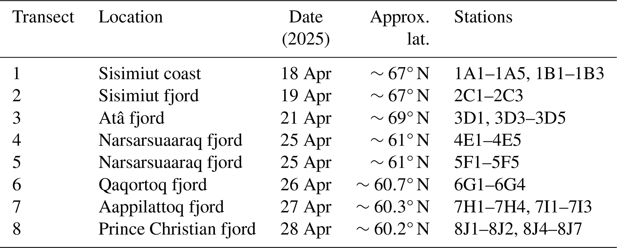
Table 3 FANS fjord transects (cruise CC170425, April 2025). Station groups follow the identifier scheme used throughout this paper. Profiles n counts only the ocean profiles retained in the final dataset.

A total of 73 ocean profiles were retained in the final dataset: 32 from SIMSVAL and 41 from FANS (Table 2).

Eight fjord transects were occupied between 18 and 28 April 2025, beginning with the Sisimiut and Atâ fjord systems in the north (67–69° N) before progressing southward to the Cape Farewell region (∼60° N; Table 3). The sampled fjords were: Sisimiut coast and fjord (∼67° N; station groups A, B, C), Atâ fjord (∼69° N; group D), Narsarsuaq fjord (Tunuillarfik; ∼61° N; group E), Narsarsuaaraq fjord (∼61° N; group F), Qaqortoq fjord (∼60.7° N; group G), Aappilattoq fjord (∼60.3° N; groups H and I), and Prince Christian fjord (∼60.2° N; group J).

2.4 Deployment method

All fjord CTD profiles were obtained using zodiac-based deployments from Le Commandant Charcot, enabling operations in shallow and near-shore fjord environments inaccessible to the main vessel. Priority was given to cross-fjord transects designed to capture the spatial variability of hydrographic conditions across the freshwater gradient from the glacier terminus toward the fjord mouth.

The deployment system consisted of a manual winch with 150 m of rope, a pulley and support bar mounted on the zodiac, and a weight attached to the lower end of the CTD to ensure vertical descent. Upon arrival at each station, the CTD was powered on and immersed at the surface for approximately 30 seconds to allow sensor stabilisation before the downcast was initiated at a controlled speed not exceeding 0.5 m s⁻¹. Surface water samples were collected in parallel in 38 stations, and measured later at laboratory of ICM-CSIC. Only downcast data were retained for processing; upcast data were discarded due to potential wake and disturbance effects.

Potential short-term vertical motions associated with Zodiac movement or manual winch operation were subsequently identified from the CTD pressure-derived vertical velocity and handled during the signal conditioning (Sect. 4.3) and the loop-removal step described in Sect. 4.4.

3 Instrumentation and data acquisition

3.1 RBR Concerto³ CTD – 16 Hz

The primary instrument was an RBR Concerto³ fast-sampling CTD (serial number 237957; ICM-CSIC) operating at 16 Hz (62.5 ms sampling period). It measures conductivity, temperature, and pressure with the following factory-stated uncertainties: temperature ±0.002 °C, conductivity ±0.003 mS cm⁻¹, pressure ±0.05 % full scale. The instrument was calibrated by RBR Ltd. prior to the SIMSVAL campaign. No post-deployment calibration drift was detected over the two-month deployment period based on the inter-sensor comparison described in Sect. 6.2.

3.2 RBR Concerto³ CTD – 2 Hz

A second RBR Concerto instrument (serial number 237329; PONANT) sampled at 2 Hz (500 ms period). Sensor specifications are identical to the 16 Hz instrument. The temperature channel is labeled Temperature1 in the RBR Ruskin database and was systematically renamed to Temperature immediately after each RSKreadprofiles call to maintain compatibility with RSKtools internal functions (Sect. 4).

3.3 Atmospheric measurements

Atmospheric pressure was measured continuously by two independent sensors aboard Le Commandant Charcot at 1 min interval. Hourly means were computed and matched to each CTD profile by nearest-time interpolation, enabling sea-pressure derivation (Sect. 4.1). Wind speed, wind direction, and relative humidity were also recorded and are included as auxiliary variables in the dataset.

4 Data processing and quality control

All processing was performed using RSKtools v3.6 (RBR Ltd.) combined with custom MATLAB routines developed for this dataset with workflow outlined in Fig. 2. The resulting product corresponds to Level 2 (georeferenced data with derived variables and automated quality control) following CF-1.8, ACDD-1.3, and SeaDataNet conventions. All QC flags derive exclusively from the automated tests described in Sect. 4.6.

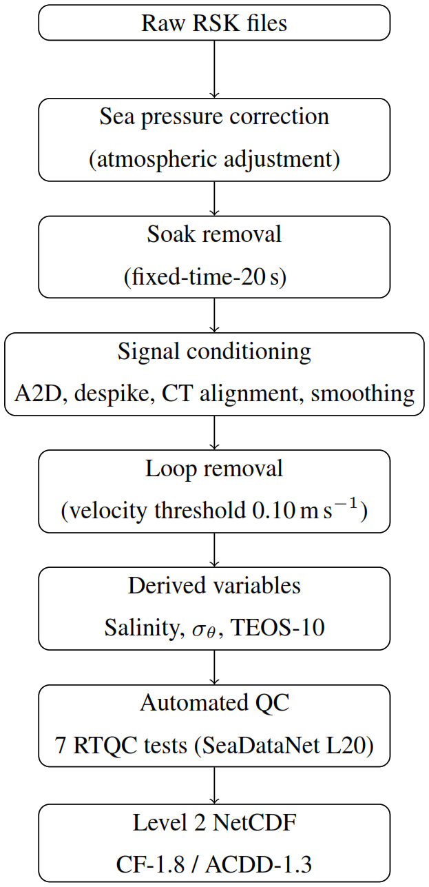
Figure 2 Level 2 processing workflow applied to the ARICE 2025 CTD profiles. Steps 1–8 are described in Sect. 4.

4.1 Sea pressure derivation

The raw CTD pressure includes atmospheric pressure. Sea pressure was derived as:

$$\begin{array}{}\text{(1)}& P_{\mathrm{sea}}=P_{\mathrm{raw}}-P_{\mathrm{atm}},\end{array}$$

where P_atm is the contemporaneous atmospheric pressure from the onboard FerryBox weather station. When atmospheric measurements were unavailable, the standard value of 10.1325 dbar was applied. All subsequent processing steps use sea pressure.

4.2 Soak phase removal

Prior to active profiling, the CTD remained immersed near the surface to allow thermal and conductivity stabilisation. The soak phase was removed by discarding the first 20 s of each cast (RSKtrim_soak_auto, fixed_time mode), applied uniformly to all 73 profiles regardless of campaign or sensor frequency. This fixed-time approach was adopted for its reproducibility and simplicity: the consistent ship-side deployment procedure and manual information ensured that a 20 s immersion period was always available, and a predetermined window removes any dependence on instantaneous descent velocity, which can vary among casts.

Two profiles (1A_1 and 7H_4) required shorter windows of 5 s via station-specific overrides, owing to an unusually rapid initial descent that began from the very moment of water entry, leaving no time for a standard pre-cast stabilization period. No minimum-depth threshold was enforced (min_soak_depth = 0): the first retained observation corresponds to the sensor position at the soak endpoint, whose depth varies by cast.

Independent near-surface water samples were also collected during the campaigns and are described in Sect. 4.8, where they provide an external reference for evaluating the uppermost salinity values retained after processing.

4.3 Signal conditioning

After soak removal, profiles underwent:

• Zero-order hold correction (RSKcorrecthold): A2D staircase artefacts replaced by linear interpolation.

• Despiking (RSKdespike): temperature and conductivity spikes flagged via a 4σ threshold in a 15-point moving window; flagged values set to NaN.

• Conductivity–temperature alignment (16 Hz only, RSKalignchannel): the thermal response lag (Δt≈0.06 s) was estimated from RSKcalculateCTlag over 5–30 dbar and applied to correct salinity spiking. Not applicable at 2 Hz (insufficient temporal resolution).

• Low-pass smoothing (RSKsmooth): 5-point moving average on temperature and conductivity to reduce high-frequency electronic noise.

4.4 Loop removal

Data segments where vertical velocity fell below 0.10 m s⁻¹ were removed using RSKremoveloops to eliminate artefacts from winch pauses, minor profile reversals or short-term vertical motions of the CTD potentially induced by Zodiac movement. This procedure ensures that only continuously descending portions of the downcast are retained for the calculation of the final hydrographic variables.

4.5 Derived thermodynamic variables

Practical salinity S_P (PSS-78) was derived from temperature and conductivity. Potential density anomaly σ_θ was computed using TEOS-10 (GSW toolbox). Absolute Salinity S_A and Conservative Temperature Θ were derived.

4.6 Automated quality control

Quality control followed a Real-Time Quality Control (RTQC) framework consistent with QARTOD (IOOS, 2020), Argo (Argo Data Management Team, 2022), and SeaDataNet L20 (SeaDataNet, 2010) recommendations. No Delayed-Mode Quality Control (DMQC) was applied. Seven automated tests were executed:

1. NaN check: flag 9 (Missing) for absent values.

2. Gross range test: global physical limits (T: −5 to 50 °C; S_P: 0 to 45 PSU; p: 0 to 12 000 dbar).

3. Regional range test: Arctic-specific limits (T: −2 to 15 °C; S_P: 20 to 36 PSU; p: 0 to 500 dbar).

4. Flat line test: flags stuck sensor readings.

5. Gradient test: $|\mathrm{d}T/\mathrm{d}p|>\mathrm{2}$ °C dbar⁻¹ or $|\mathrm{d}S/\mathrm{d}p|>\mathrm{1}$ PSU dbar⁻¹.

6. Density inversion test: ${\mathit{\sigma }}_{\mathit{\theta }}(n+\mathrm{1})<{\mathit{\sigma }}_{\mathit{\theta }}\left(n\right)-\mathrm{0.03}$ kg m⁻³.

7. Pressure monotonicity check: non-monotone sequences flagged Suspect.

The gross range test serves as a first-pass check for physically impossible values indicative of sensor malfunction; all observations in this dataset fall well within these limits. The regional limits were selected to encompass the broad range of hydrographic conditions expected across Arctic and sub-Arctic fjord environments, including highly fresh glacier-influenced surface waters and saline Atlantic-origin waters. Separate thresholds were not defined for individual fjords because the sampled regions exhibit strongly contrasting hydrographic regimes, and more restrictive local limits could incorrectly flag physically plausible observations. Automated QC flags were therefore used as indicators rather than exclusion criteria, and all original values were retained in the dataset. Flags were not used to remove data; original values are preserved in the NetCDF with their associated flags, enabling users to apply custom filtering. Profiles with soak depth > 10 dbar received Suspect flags at the surface layer. QC performance statistics are reported in Sect. 6.1.

4.7 Frequency-specific processing differences

The sampling frequency was auto-detected from the RBR database field rsk.continuous.samplingPeriod (ms), with per-station overrides where needed. CT lag correction and hold-error correction were applied only to 16 Hz data. All time-window parameters were scaled to maintain equivalent physical timescales (Table 4).

Table 4 Processing parameters by sampling frequency.

4.8 Discrete salinity samples (AutoSal)

At each station, a near-surface water sample was collected from the upper 0–10 cm layer using 200 mL sampling tubes. The samples were immediately sealed with Parafilm and stored until laboratory analysis at the ICM using a Guildline Autosal 8400B salinometer (precision ± 0.001 PSU relative to IAPSO Standard Seawater). These discrete salinity measurements are included in the dataset as a complementary variable and are presented in the scientific context section (Sect. 5.3.1). Their inclusion specifically provides information on the very near-surface layer, which may be of interest for studies focused on air–sea interactions, freshwater lenses, and upper-ocean stratification.

Figure 3 shows selected examples from different hydrographic regions, illustrating how the discrete AutoSal samples complement the CTD profiles by providing an independent estimate of the very near-surface salinity. The comparison highlights the strong spatial variability of the uppermost salinity field, including both well-mixed profiles and stations with sharp near-surface gradients or fresh surface lenses.

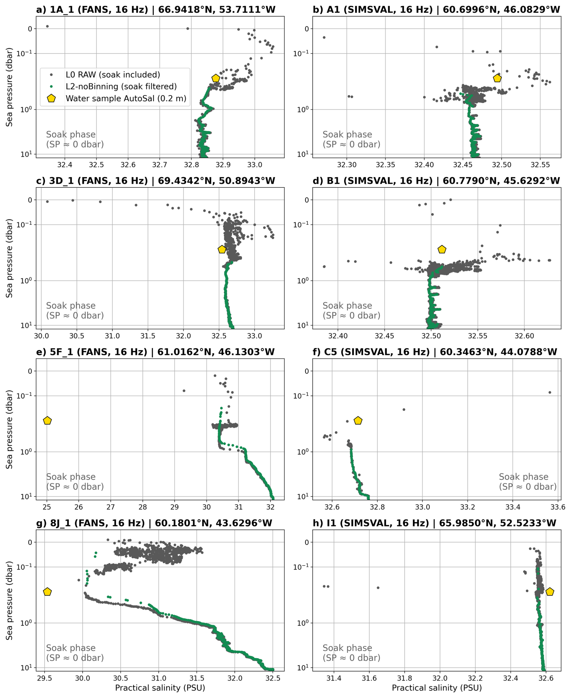
Figure 3 Near-surface salinity comparison for selected stations representative of different hydrographic settings sampled during the FANS and SIMSVAL campaigns. Grey dots show the raw low-resolution CTD practical salinity measurements, including the initial soak phase, while green profiles correspond to the filtered salinity profiles retained in the final dataset. Yellow diamonds indicate the discrete near-surface salinity samples measured with the Guildline Autosal 8400B salinometer at approximately 0.2 m depth. Sea pressure y axis is shown in symmetric logarithmic scale to improve the visualization of the first meters of the water column.

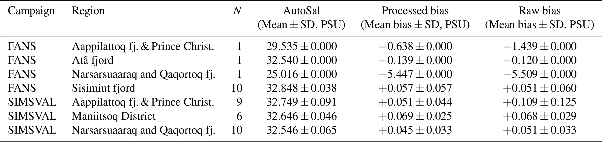
To quantify these differences, Table 5 summarizes the mean bias and standard deviation between the discrete AutoSal samples and the corresponding soak-filtered CTD salinity values, grouped by campaign and sampling area. This regional grouping allows the comparison to account for the strong spatial variability of near-surface salinity rather than treating all stations as a single homogeneous dataset.

Table 5 Mean near-surface salinity and statistical comparison of biases (computed as S_AutoSal−S_CTD) grouped by campaign and region (Fig. 1), expressed as mean bias ± the standard deviation (SD) of regional measurements. Biases are evaluated using the first available depth of filtered processed profiles and the average raw surface data within the top 3.0 dbar. N denotes the number of discrete AutoSal samples per campaign and region.

5 Dataset description

5.1 Overview and spatial coverage

The dataset consists of 73 quality-controlled CTD profiles (Table 2): 32 from SIMSVAL and 41 from FANS. Each profile spans 0–∼150 dbar on the nominal vertical resolution. Actual maximum profiling depths range from 5.1 to 148.9 dbar, depending on local bathymetry and operational conditions. Complete per-profile metadata, including acquisition date and time (UTC), geographic coordinates, maximum pressure, and instrument sampling frequency, are provided in Tables A1 and A2.

To facilitate the regional interpretation of hydrographic variability, the profiles were grouped into the geographical sectors defined in Fig. 1. Figure 4 presents the vertical distributions of conservative temperature, absolute salinity, and the ratio between the thermal expansion and saline contraction ($\mathit{\alpha }/\mathit{\beta }$) for each sector (areas B–F). The $\mathit{\alpha }/\mathit{\beta }$ ratio provides a measure of the relative contribution of temperature and salinity to density variations: low values indicate salinity-dominated density variability, whereas higher values indicate an increasing thermal contribution.

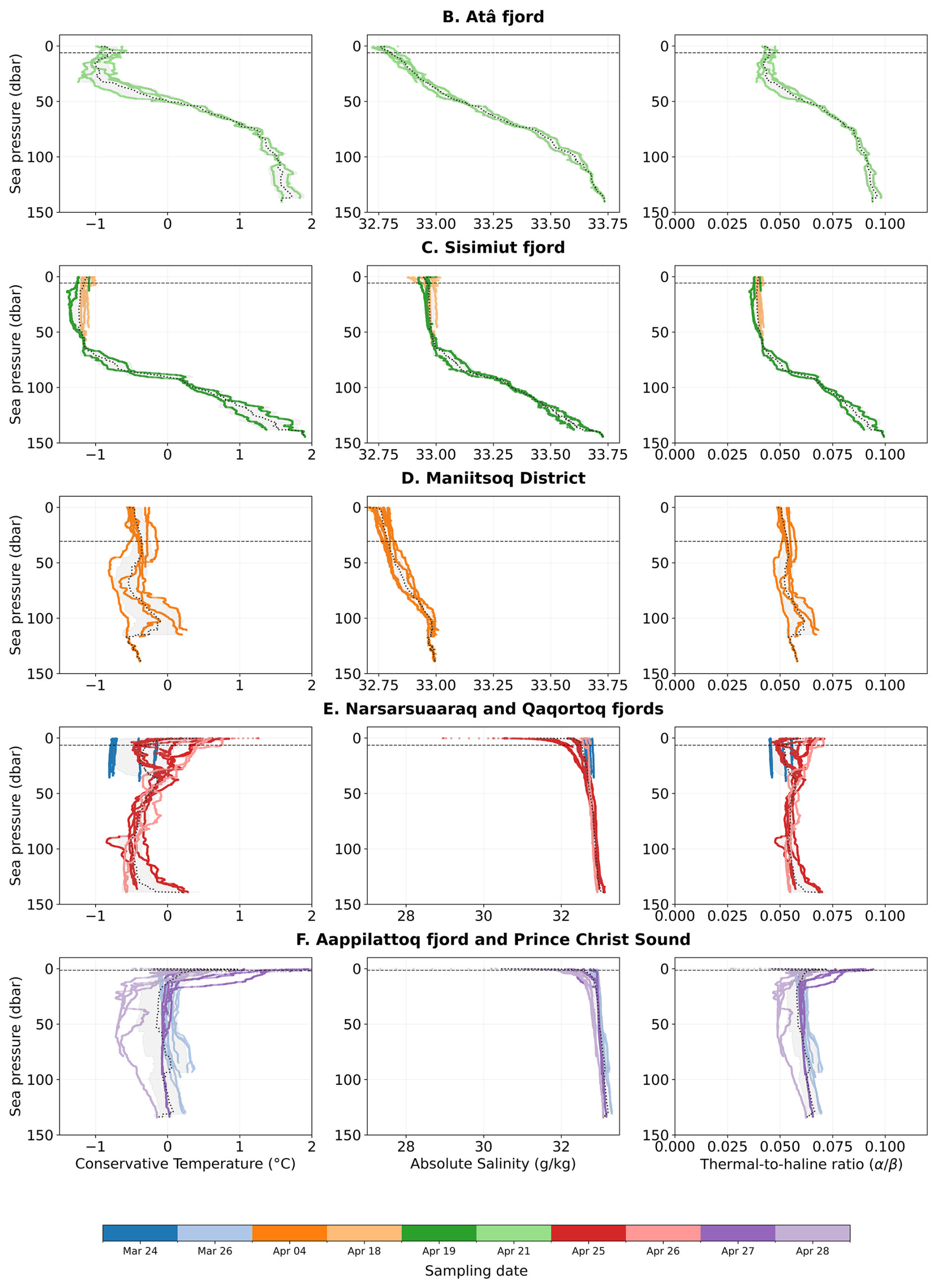
Figure 4 Vertical profiles by region (areas B–F in Fig. 1) of conservative temperature (left panels), absolute salinity (centre panels), and the ratio of thermal expansion to saline contraction coefficients ($\mathit{\alpha }/\mathit{\beta }$) (right panels). Individual casts are coloured by sampling date. The grey shaded band represents the standard deviation around the regional mean profile (grey dotted line). The black dashed line indicates the median pycnocline depth, defined as the depth of maximum buoyancy frequency squared (N²; Brunt–Väisälä stability criterion) across profiles within each region.

Area B is characterised by relatively warm and saline subsurface waters, with conservative temperature increasing from near-freezing surface conditions to >1.5 °C below ∼70–100 dbar and absolute salinity exceeding 33 g kg⁻¹. The $\mathit{\alpha }/\mathit{\beta }$ ratio increases with depth, indicating that temperature becomes progressively more important for density variations in the subsurface layer.

Area C exhibits a marked two-layer structure, including a shallow fresh surface layer overlying warmer and saltier subsurface waters. The strongest salinity gradients occur within the upper ∼10–20 m. The low $\mathit{\alpha }/\mathit{\beta }$ values in the upper layer indicate that density variability is mainly controlled by salinity, while the increase with depth reflects a greater thermal contribution below the pycnocline.

Area D shows colder and fresher conditions overall, together with enhanced profile-to-profile variability, particularly within the upper ∼50 m where strong near-surface salinity gradients are observed. The relatively low $\mathit{\alpha }/\mathit{\beta }$ values indicate a predominantly salinity-controlled density structure, consistent with strong freshwater influence and stratification.

Areas E and F display the widest hydrographic range of the dataset, including extremely fresh near-surface layers associated with meltwater and coastal freshwater inputs. In several profiles, these freshwater lenses are confined to the upper few metres, producing very sharp near-surface stratification. In these sectors, very low near-surface $\mathit{\alpha }/\mathit{\beta }$ values indicate that density variability in the upper layer is strongly dominated by salinity rather than temperature.

Across all regions, the updated near-surface processing reveals that the strongest hydrographic variability is concentrated within the upper few metres, where thin freshwater lenses and sharp pycnoclines frequently develop during spring.

The grey shaded regions in Fig. 4 represent the standard deviation of all profiles around the regional mean (grey dotted line), providing a reference for the hydrographic variability sampled within each region. The black dashed line indicates the median pycnocline depth, defined as the depth of maximum buoyancy frequency squared (N²) across profiles in each sector, highlighting the shallow stratification characteristic of several glacier-influenced regions.

5.2 File format and conventions

The NetCDF-4 file follows CF Conventions v1.8 (CF Conventions Committee, 2020) and ACDD v1.3 (ESIP Federation, 2015). Compliance was verified with the IOOS cfchecker tool (0 errors, 0 warnings). The file uses a 2D structure (depth × profile) with fill value NaN for missing data.

The file contains n_profile=73 profiles (32 SIMSVAL and 41 FANS), stored at native temporal resolution in a two-dimensional (obs × profile) structure. The obs dimension equals the maximum sample count across all profiles; arrays are NaN-padded beyond each profile's valid sample count (n_samples). There is no common pressure grid: each sample carries its own sea_pressure value, spanning from the near-surface to a profile-dependent maximum depth (5.1–148.9 dbar for FANS; 10.6–145.9 dbar for SIMSVAL). Time is encoded as seconds since 1 January 1970, 00:00:00Z (UTC), both as a per-profile scalar (time) and as a per-sample array (sample_time).

5.3 Variable definitions

The NetCDF file (SIMSVAL_FANS_MarApr2025_PROC. nc) contains the following variables (Table 6):

• Measured: temperature T (°C, ITS-90), conductivity C (S m⁻¹), the absolute pressure P_raw (dbar).

• Derived: sea-water pressure P_sea (dbar) – raw pressure minus ship atmospheric pressure (P_atm, from Ferrybox), practical salinity S_P (PSS-78), potential density anomaly σ_θ (kg m⁻³, TEOS-10), descent velocity w (m s⁻¹).

• Coordinates: per-profile deployment time (time, POSIX s), per-sample time (sample_time, POSIX s), latitude (° N), longitude (° E), station identifier, campaign label (SIMSVAL or FANS).

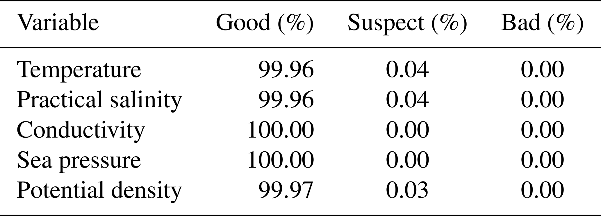
• QC flags: SeaDataNet L20 integer flags for T, C, S_P, σ_θ, and p (1 = Good, 3 = Suspect, 4 = Bad, 9 = Missing/NaN-padding fill).

• Soak metadata: soak duration`(s), soak depth (dbar), number of samples removed during soak trimming.

• Sampling info: number of valid samples per profile (n_samples), nominal sampling frequency (Hz).

• Atmospheric: ship atmospheric pressure from two independent sensors (hPa), wind speed and direction, relative humidity.

• Complementary: near-surface water sample salinity (sss, PSS-78), collected by zodiac at ∼0.2 m depth (Guildline Autosal 8400B, ±0.001 PSU).

Table 6 NetCDF variable summary for (SIMSVAL_FANS_MarApr2025_PROC.nc) (v5 L2, 73 profiles). Dimensions: obs = maximum sample count across all profiles (arrays NaN-padded); profile = 73.

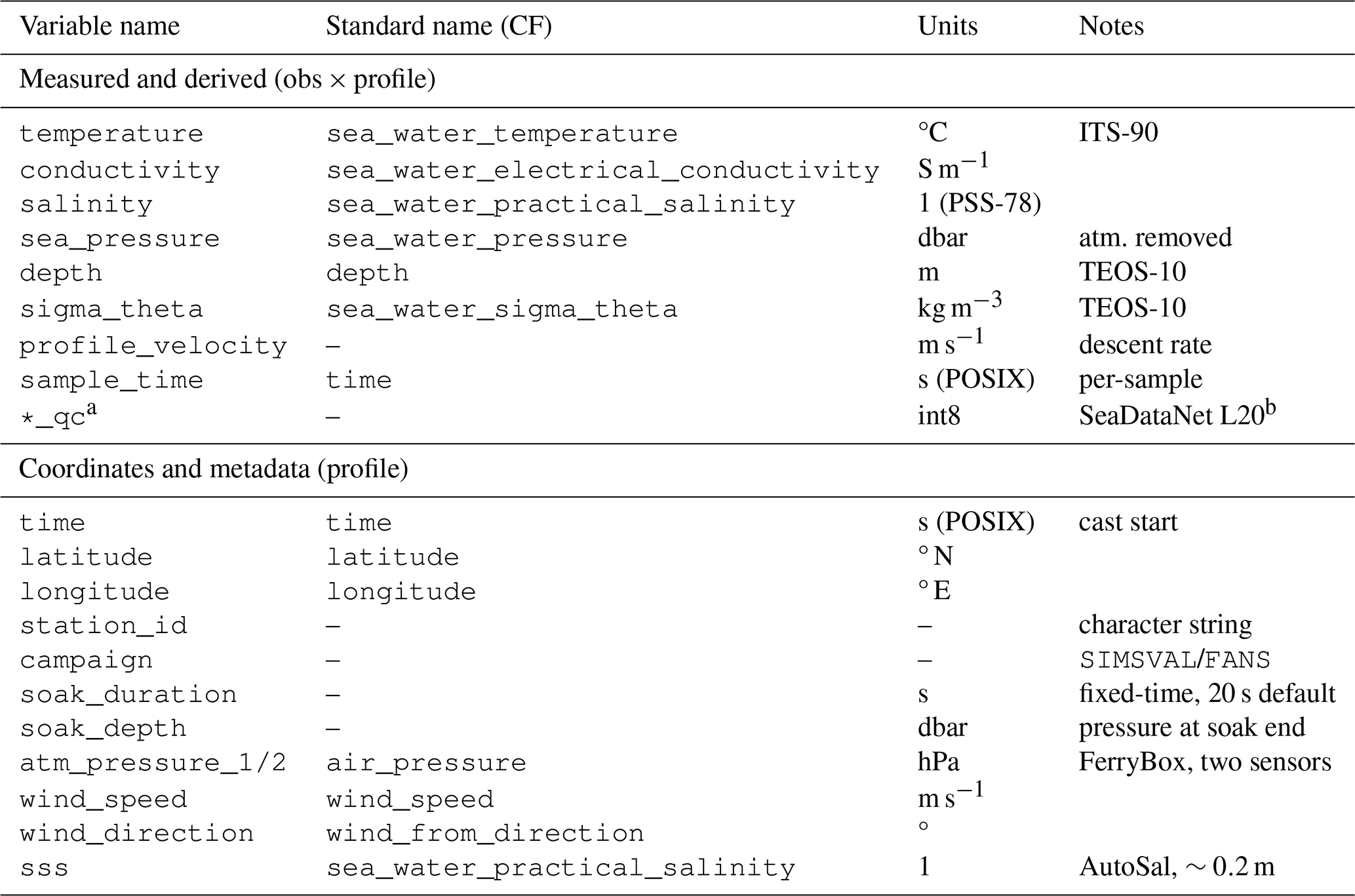
^a Five QC flag variables: temperature_qc, conductivity_qc, Salinity_qc, sigma_theta_qc, sea_pressure_qc. ^b 1 = Good, 3 = Suspect, 4 = Bad, 9 = Missing/padding.

Near-surface salinity: AutoSal Niskin bottle samples

At each station, a discrete water sample was collected at 0.2 m depth by Niskin bottle and analysed with a Guildline Autosal 8400B salinometer (precision ± 0.001 PSU relative to IAPSO Standard Seawater). These measurements are included in the dataset as a complementary variable and are presented here alongside the CTD profiles to characterise the near-surface salinity structure.

These discrete samples cannot serve as a formal validation reference for the CTD salinity at the shallowest valid bin (∼1 dbar). West Greenland fjords develop intense near-surface haloclines with vertical gradients of order 0.5–4 PSU m⁻¹ within the upper 6–10 m during the melt onset in March–April (Mortensen et al., 2013; Stuart-Lee et al., 2021; Meire et al., 2019). At these gradients, the 0.5 m depth offset between the Niskin closure and the CTD first valid bin implies an expected natural salinity difference of 0.25–2 PSU – more than two orders of magnitude larger than the RBR Concerto salinity accuracy (±0.003 PSU). Furthermore, atmospheric forcing (rainfall, surface meltwater) generates sub-metre salinity stratification on sub-hourly timescales (Drushka et al., 2016), and Niskin bottle sampling in a strong vertical salinity gradient is subject to entrainment and flushing biases (Paver et al., 2020). Standard GO-SHIP and HOT protocols explicitly prefer bottle samples from deep, homogeneous water for CTD conductivity calibration, and flag near-surface samples as having inherently higher uncertainty (Argo Data Management Team, 2022; IOOS, 2020).

6 Technical validation

6.1 Quality control performance

Among non-missing values, 99.99 % of temperature, 99.94 % of salinity, 100.00 % of conductivity, and 100.00 % of sea pressure measurements received flag 1 (Good, Table 7). No data were flagged 4 (Bad). Suspect flags (flag 3) represent <0.1 % of non-missing values across all variables and are concentrated in the upper 10 dbar, primarily associated with density inversions from near-surface meltwater lenses (density inversion test) and near-surface salinity gradients (gradient test).

Table 7 QC flag distribution (% of non-missing data).

6.2 Inter-sensor comparison (16 Hz vs. 2 Hz)

Inter-sensor consistency was assessed using a simultaneous validation cast performed at Station B (60.78° N, 45.63° W) during SIMSVAL. The PONANT instrument (RBR Concerto, 2 Hz, S/N 237329) was deployed 1.4 min after the ICM-CSIC instrument (RBR Concerto³, 16 Hz, S/N 237957) at the same location (distance < 0.01 km). The results presented here should therefore be interpreted as a field-based of inter-sensor consistency rather than a formal evaluation of sensor accuracy. No pre-cruise laboratory intercomparison was possible because the PONANT instrument was not available before the campaigns, and no simultaneous side-by-side deployment was conducted.

The comparison was conducted in two steps to distinguish instrumental offsets from processing-induced differences. irst, raw temperature and conductivity data were compared directly, without any correction, soak removal, or quality-control filter. The ICM profile (16 Hz) was linearly interpolated onto the PONANT native pressure levels (2 Hz) over the 2–10 dbar window (N=59 points), to avoid sensor acclimation effects. The raw inter-sensor biases (PONANT − ICM) are $\mathrm{\Delta }T=+\mathrm{0.0008}$ °C (SD = 0.0024 °C) and $\mathrm{\Delta }C=-\mathrm{0.0098}$ mS cm⁻¹ (SD = 0.0031 mS cm⁻¹, Table 8). Both values fall within or very close to the manufacturer-specified precision of the RBR Concerto sensors (±0.002 °C for temperature, ±0.003 mS cm⁻¹ for conductivity), confirming that the offset is primarily of instrumental origin rather than introduced by the processing chain.

After applying the full post-processing pipeline (pressure correction, hold-event removal, CT-lag alignment, despiking, smoothing, and soak- and loop-phase removal), comparison of the processed profiles (N=31 QC-good points between 2 and 10 dbar) yielded $\mathrm{\Delta }T=+\mathrm{0.0028}$ °C (SD = 0.0014 °C), $\mathrm{\Delta }C=-\mathrm{0.0107}$ mS cm⁻¹ (SD = 0.0021 mS cm⁻¹), and $\mathrm{\Delta }S=-\mathrm{0.017}$ PSU (SD = 0.0029 PSU).

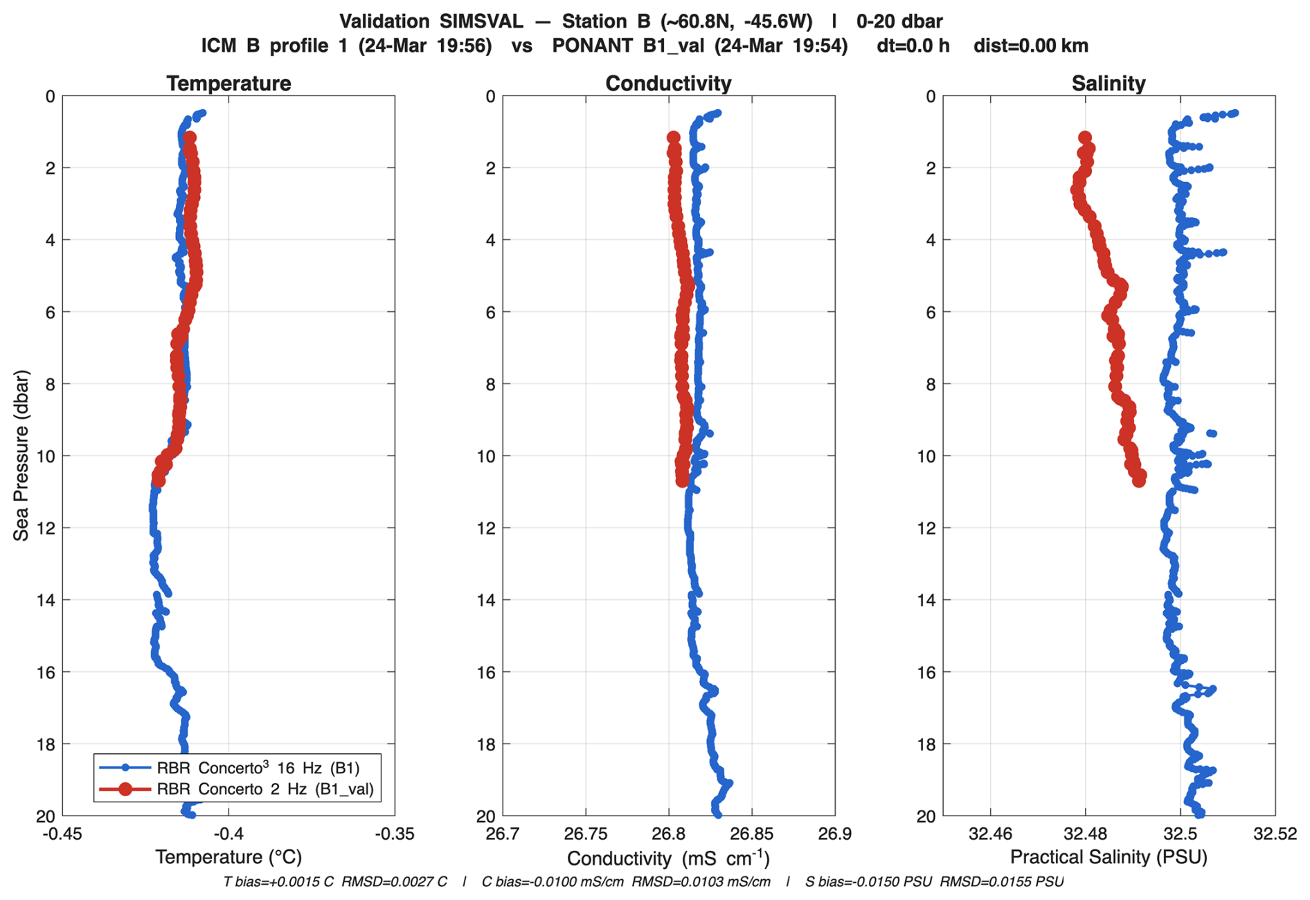
Figure 5 Inter-sensor comparison: temperature (left panel), conductivity (centre panel), and practical salinity (right panel) profiles from the simultaneous SIMSVAL co-deployment at station B1 (24 March 2025, Δt=1.4 min). Blue: RBR Concerto³ – 16 Hz; red: RBR Concerto – 2 Hz.

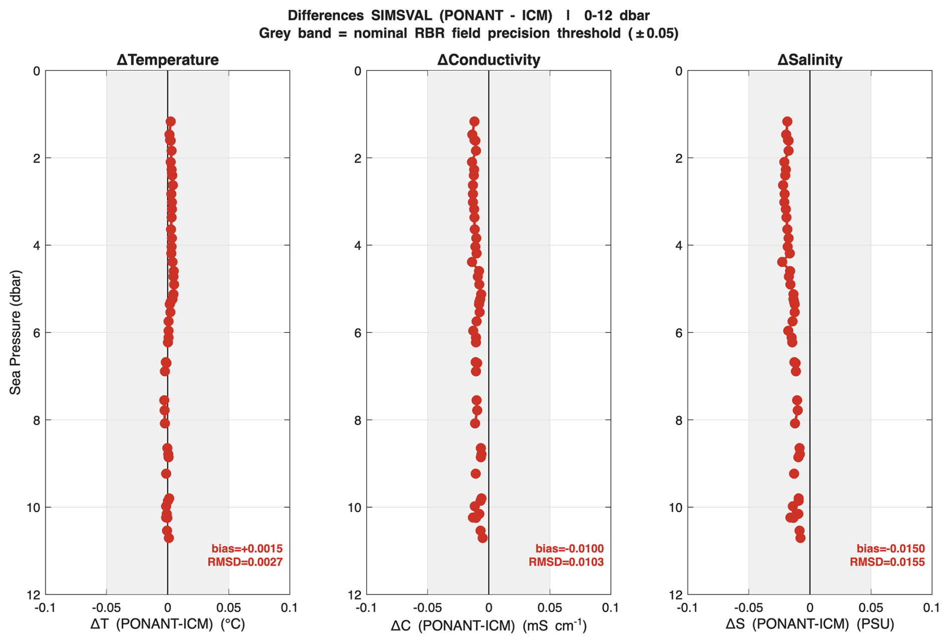
Figure 6 Profile differences between the two RBR Concerto CTDs (2 and 16 Hz) for temperature (left panel), conductivity (centre panel), and practical salinity (right panel). The grey band indicates the nominal RBR sensor precision (±0.05 for the indicative field comparison threshold). Mean bias and SD are annotated on each panel.

Table 8 Inter-sensor validation between the two RBR CTD (2–16 Hz), mean bias ± SD over good-flagged data only shown in Figs. 5 and 6). SIMSVAL station B1 is the only pair with verified quasi-simultaneous co-location.

The slightly larger bias and scatter in the processed comparison most likely reflect differences in processing and sampling conditions rather than intrinsic disagreement between the sensors. First, the CT-lag correction, applied only to the 16 Hz ICM sensor, shifts the conductivity channel by approximately one scan (∼0.06 s), potentially introducing a small offset when conductivity measurements from the two instruments are compared at identical pressure levels. Second, the 1.4 min delay between the casts means that the instruments sampled slightly different water parcels, particularly within the near-surface layer where temperature and salinity gradients are strongest. Over this time interval, tidal oscillations and internal waves may have displaced the pycnocline by several decimetres, producing apparent inter-sensor differences that reflect genuine oceanographic variability rather than sensor bias. Consequently, a substantial fraction of the residual scatter (SD ≈ 0.003–0.018 across variables) is likely attributable to short-term environmental variability rather than instrumental differences.

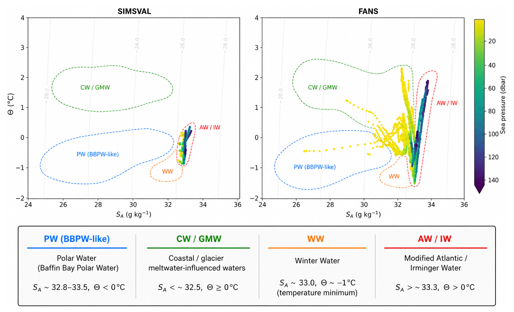
Figure 7 Conservative temperature–absolute salinity (Θ–S_A) diagrams for the SIMSVAL (March 2025) and FANS (April 2025) campaigns. Colours indicate sea pressure (dbar). Dashed envelopes indicate the approximate thermohaline domains of modified Atlantic/Irminger Water (AW/IW), Winter Water (WW), Polar Water or Baffin Bay Polar Water-like waters (PW/BBPW-like), and coastal/glacier meltwater-influenced waters (CW/GMW). Compared with SIMSVAL, the FANS profiles show a broader near-surface spread toward lower salinity and warmer conservative temperature, consistent with the onset of early-spring meltwater input, runoff, and surface restratification.

Although ΔC and ΔS slightly exceed the nominal single-instrument precision of the RBR Concerto (±0.003 PSU), the observed discrepancies remain well within the recommended field-comparison thresholds (±0.05 °C and ±0.05 PSU). Moreover, they are more than an order of magnitude smaller than the hydrographic variability observed across the Greenland fjords (ΔT∼3 °C and ΔS∼3 PSU over 0–150 dbar). Overall, the agreement between the two instruments is considered fully adequate for the objectives of this dataset.

6.3 Thermohaline diagnostics and hydrographic regimes

Figure 7 presents the Θ–S_A diagrams separated by expedition leg, allowing comparison between the late-winter conditions sampled during SIMSVAL (March 2025) and the early-spring conditions sampled during FANS (April 2025). The diagrams provide a thermohaline framework for interpreting the main water-mass regimes sampled across Southwest Greenland fjords. The dashed envelopes are intended as approximate hydrographic regimes and mixing end-members, rather than strict water-mass boundaries.

Both campaigns exhibit coherent thermohaline structures, with observations distributed along physically consistent mixing branches. This confirms the internal consistency of the processing workflow and of the TEOS-10-derived variables. The most saline and relatively warm branch corresponds to modified Atlantic-origin waters associated with Irminger Water inflow (AW/IW), characterized in this dataset by S_A>33.3 g kg⁻¹ and positive conservative temperature. These waters occupy the deeper part of the sampled fjord water column and represent the main subsurface heat reservoir.

At intermediate salinities, the profiles converge toward a colder temperature-minimum layer centred around S_A∼33 g kg⁻¹ and $\mathrm{\Theta }\sim -\mathrm{1}$ °C, consistent with Winter Water (WW) formed by winter cooling and convective mixing. Fresher and colder waters are associated with Polar Water or Baffin Bay Polar Water-like waters (PW/BBPW-like), while the freshest and relatively warmer near-surface values correspond to coastal and glacier meltwater-influenced waters (CW/GMW).

The SIMSVAL and FANS datasets show broadly similar subsurface thermohaline properties, indicating limited changes below the near-surface layer over the approximately one-month interval between campaigns. In contrast, FANS displays a much wider spread toward low salinity and warmer surface conditions, consistent with the onset of early-spring meltwater input, runoff, and surface atmospheric warming. This contrast supports the interpretation that the strongest seasonal signal is concentrated in the upper water column, while deeper Atlantic-origin and winter-cooled waters remain comparatively stable (Mortensen et al., 2018; Rysgaard et al., 2020).

The continuity between the identified water masses suggests physically consistent mixing pathways linking polar surface waters, winter-cooled intermediate waters, and Atlantic-origin subsurface waters within the fjord systems.

6.4 Spring thermohaline transition across glacier influence regimes

To investigate the early spring thermohaline transition, CTD profiles were grouped according to their glacier influence: (i) tidewater glacier fjords, (ii) land-terminating glacier fjords, and (iii) fjords with no direct glacier influence (Fig. 8, Table 9). For each group, SIMSVAL (March) and FANS (April) profiles are compared in terms of temperature and salinity vertical structure (Figs. 9–11).

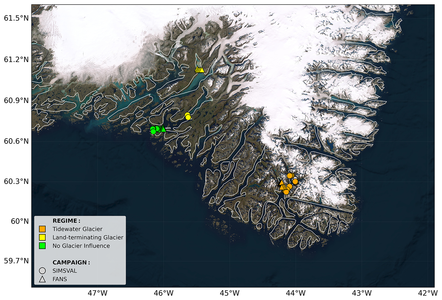
Figure 8 CTD station locations grouped by glacier influence regime. Colours indicate fjord type: tidewater glacier fjords (cyan), land-terminating glacier fjords (yellow), and fjords with no direct glacier influence (green). Circles correspond to SIMSVAL (March 2025) and triangles to FANS (April 2025). Satellite imagery background from ESRI World Imagery|Powered by Esri; coastlines in white from Natural Earth.

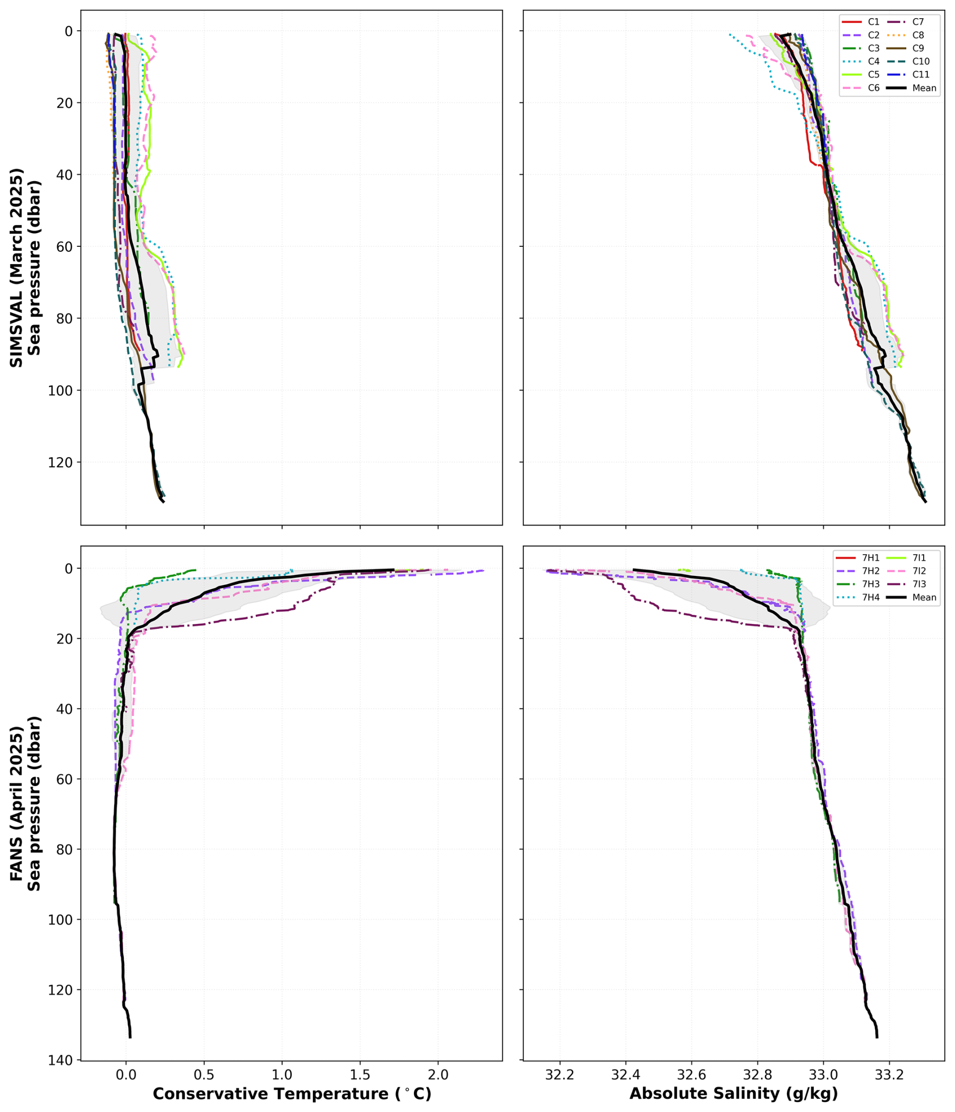
Figure 9 Vertical profiles of conservative temperature (left panels) and absolute salinity (right panels) in tidewater glacier fjords (Aappilattoq) for SIMSVAL (top panels, March 2025) and FANS (bottom panels, April 2025). Individual stations are displayed using distinct color-and-line-style combinations for accessibility and unambiguous identification. Dotted black lines and shaded areas denote the multi-station mean and standard deviation, respectively. The comparison highlights the development of a shallow, freshened and slightly warmer near-surface layer during FANS, while the deeper water column remains comparatively similar to March conditions.

Table 9 Geographic grouping of CTD profiles used to analyse the March–April thermohaline transition. Fjords are classified by glacier influence (tidewater, land-terminating, and no direct glacier influence). Sampling dates correspond to SIMSVAL (March 2025) and FANS (April 2025). n denotes the number of profiles included in each group.

The tidewater glacier group (Aappilattoq fjord) exhibits the strongest seasonal contrast between March and April (Fig. 9). During SIMSVAL (March), temperature profiles are relatively homogeneous, with weak stratification and values generally close to 0 °C throughout the upper 100 m, consistent with late-winter mixed conditions. Salinity remains relatively high (S_A≳32.6 g kg⁻¹) in the upper water column, indicating limited freshwater influence.

In contrast, FANS (April) profiles display pronounced near-surface freshening and stratification, particularly within the upper ∼1–10 m. Several stations exhibit very fresh near-surface waters, indicating the presence of a shallow meltwater lens. This surface freshening is accompanied by enhanced stratification and slight near-surface warming. Below the freshened layer, temperature and salinity progressively converge toward the March conditions, indicating that the seasonal signal is largely confined to the upper water column. This structure is consistent with the onset of glacial meltwater input and surface buoyancy forcing typical of early spring.

Profiles from fjords influenced by land-terminating glaciers show a more moderate seasonal transition than the tidewater glacier group (Fig. 10). In March, both temperature and salinity profiles are nearly vertical, indicating a relatively well-mixed water column with weak stratification.

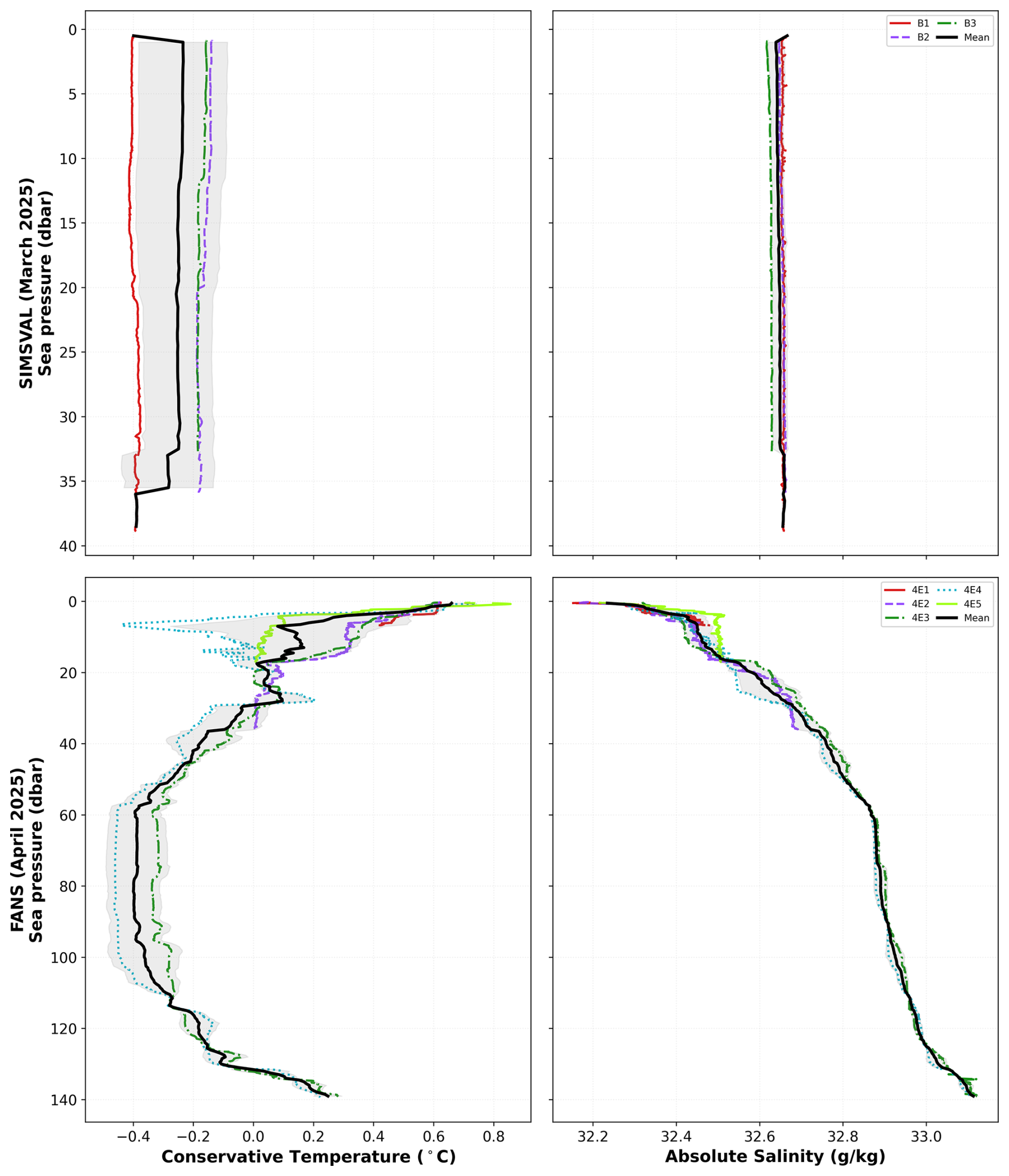
Figure 10 Vertical profiles of conservative temperature (left panels) and absolute salinity (right panels) in fjords influenced by land-terminating glaciers (Qaqortoq region) for SIMSVAL (top panels, March 2025) and FANS (bottom panels, April 2025).Individual stations are displayed using distinct color-and-line-style combinations for accessibility and unambiguous identification. Dotted black lines and shaded areas denote the multi-station mean and standard deviation, respectively.

By April, surface-intensified stratification becomes apparent. Several profiles exhibit a shallow fresh surface layer confined to the upper ∼5–15 m, overlying colder and saltier subsurface waters. Salinity generally decreases toward the surface through the upper ∼30–50 m, although the strongest gradients remain concentrated within the first few metres. Temperature profiles also show enhanced vertical structure in the upper water column, suggesting the combined influence of surface warming and freshwater input. Below ∼80 m, hydrographic properties remain comparatively stable between campaigns.

Fjords with no direct glacier influence exhibit the weakest seasonal signal among the three regimes (Fig. 11). During SIMSVAL (March), the water column is nearly homogeneous in both conservative temperature and absolute salinity, reflecting late-winter conditions dominated by vertical mixing.

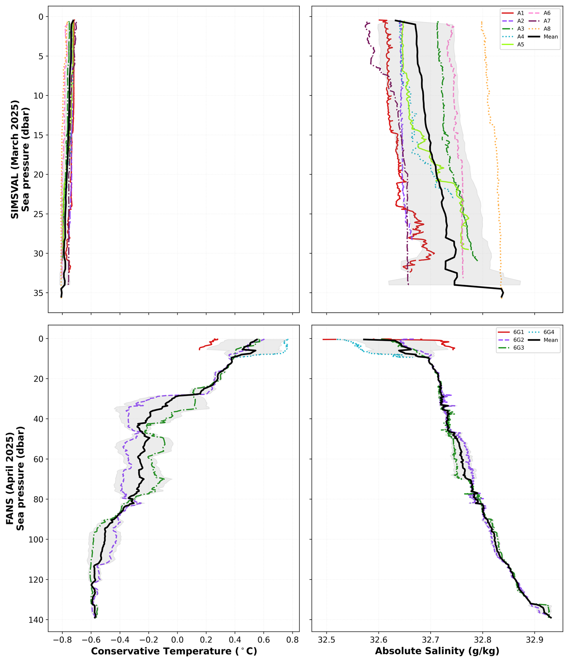
Figure 11 Vertical profiles of conservative temperature (left panels) and absolute salinity (right panels) in fjords with no direct glacier influence for SIMSVAL (top panels, March 2025) and FANS (bottom panels, April 2025). Individual stations are displayed using distinct color-and-line-style combinations for accessibility and unambiguous identification. Dotted black lines and shaded areas denote the multi-station mean and standard deviation, respectively. Compared with glacier-influenced fjords, the April profiles show weaker and less spatially coherent near-surface freshening, indicating a more moderate early-spring transition.

In April, some surface-intensified stratification develops, mainly expressed as a gradual salinity decrease toward the surface within the upper ∼30–50 m. However, the magnitude of freshening is smaller and less spatially coherent than in glacier-influenced fjords. Temperature changes are also more moderate, with no clear evidence of the strong shallow warm and fresh surface layer observed in the tidewater glacier group. This suggests that, in fjords without direct glacier input, the early-spring transition is primarily driven by regional surface forcing and coastal freshwater influence rather than local glacier-derived meltwater.

Overall, the comparison across glacier influence regimes indicates that the March–April transition is strongest in tidewater glacier fjords, moderate in fjords influenced by land-terminating glaciers, and weakest in fjords without direct glacier influence. In all cases, the main seasonal signal is concentrated in the upper water column, while deeper thermohaline properties remain comparatively stable over the one-month interval. This pattern supports the interpretation that early-spring restratification in Southwest Greenland fjords is controlled by the combined effects of local freshwater input, glacier influence, and regional surface forcing (Straneo and Heimbach, 2013; Mortensen et al., 2011).

7 Code and data availability

The CTD dataset described in this study is publicly available at Zenodo (https://doi.org/10.5281/zenodo.20489479, Hoareau et al., 2026) in NetCDF-4 format compliant with CF 1.8 and ACDD 1.3 conventions. The repository contains two complementary files: a processed Level-2 product (SIMSVAL_FANS_MarApr2025_PROC.nc, 73 profiles), including quality-control flags, derived thermodynamic variables (TEOS-10), soak metadata, auxiliary atmospheric data, and discrete AutoSal surface salinity measurements; and a native Level-0 product (SIMSVAL_FANS_MarApr2025_RAW.nc, 73 profiles), preserving the native instrument output. Data are released under the Creative Commons Attribution 4.0 International (CC-BY-4.0) licence.

All data-processing, quality-control, and validation work-flows are openly available on GitHub (https://github.com/Barcelona-Polar-Lab/SIMSVAL_FANS_MarApr2025_postprocessing, last access: 2 April 2026), with a citable archived version on Zenodo (https://doi.org/10.5281/zenodo.20527364, Hoareau, 2026). The repository contains documented MATLAB scripts sufficient to reproduce the full processing chain and all validation figures presented in this paper.

8 Conclusions

We present a dataset of 73 quality-controlled CTD profiles from Southwest Greenland fjords (60.2–69.5° N), collected during two late-winter to early-spring 2025 campaigns (SIMSVAL, 24 March–4 April; FANS, 18–28 April) aboard Le Commandant Charcot. The profiles were processed through a reproducible workflow based on RSKtools and TEOS-10, original vertical resolution, and quality-controlled with seven automated tests following QARTOD, Argo, and SeaDataNet L20 recommendations. More than 99.96 % of temperature and salinity measurements were flagged Good, with no Bad values detected, indicating a high level of data reliability.

A key feature of this dataset is the preservation of the shallowest valid measurements and of QC-flagged Suspect values, rather than applying an automatic filtering of the near-surface layer. This is particularly important in glacier-influenced fjords, where meltwater lenses, sharp haloclines, and density inversions are often confined to the upper few metres. These structures are commonly missed or under-resolved by standard ship-based CTD surveys, which often exclude the uppermost meters during processing, and by autonomous platforms such as Argo floats, which cannot operate in shallow, narrow, and ice-affected fjord environments. Retaining these near-surface observations therefore allows the dataset to resolve meltwater-driven stratification that would otherwise remain poorly documented.

Inter-sensor comparison from a quasi-simultaneous co-deployment demonstrates excellent agreement between instruments, with temperature, conductivity, and salinity biases well within nominal sensor precision. Thermohaline diagnostics confirm the presence of the expected regional hydrographic regimes, including coastal and glacier meltwater-influenced waters, Polar or Baffin Bay Polar Water-like waters, Winter Water, and modified Atlantic or Irminger Water. These regimes reveal physically consistent mixing structures, supporting the internal thermodynamic coherence of the dataset.

Beyond its technical quality, the dataset captures the onset of the late-winter to early-spring thermohaline transition in Southwest Greenland fjords. The comparison between March and April observations shows the development of a freshened and stratified surface layer, while deeper water masses remain comparatively stable. This transition is strongest in fjords directly influenced by tidewater glaciers and progressively weaker in systems with reduced or absent glacier input, highlighting the dominant role of freshwater forcing in shaping early-season stratification.

The dataset provides new observations of hydrographic conditions in several remote and sparsely sampled fjords of Southwest Greenland during the late-winter to early-spring period, when in situ measurements are limited and access can be restricted by sea ice and harsh weather conditions. By resolving and preserving the upper few metres of the water column, the dataset documents shallow meltwater signals and near-surface stratification processes relevant to local fjord freshwater dynamics, glacier–ocean interactions, and seasonal hydrographic evolution.

The combination of high-quality measurements, consistent processing, near-surface data preservation, and open availability provides a robust resource for studies of fjord dynamics, freshwater pathways, glacier–ocean interactions, and Arctic coastal stratification, as well as for the evaluation of ocean models and satellite-derived products. By documenting both the vertical structure of fjord water masses and their seasonal transition during the onset of spring, this dataset provides a valuable reference for future observational and modeling efforts in a rapidly changing cryosphere–ocean system.

Appendix A: Station coordinates and metadata

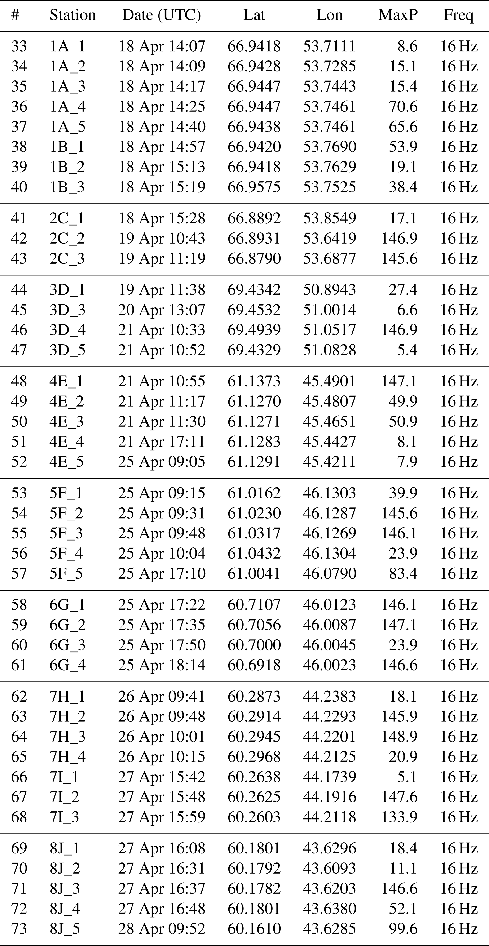
Tables A1 and A2 list the full metadata for all 73 CTD profiles in the dataset: profile index within the combined file, station identifier, date and time (UTC), geographic coordinates, maximum valid pressure, and sampling frequency.

Table A1 SIMSVAL profile metadata (cruise CC210325, March–April 2025). Longitude is given as degrees West (° W). MaxP: maximum valid sea pressure. Freq: RBR sampling frequency.

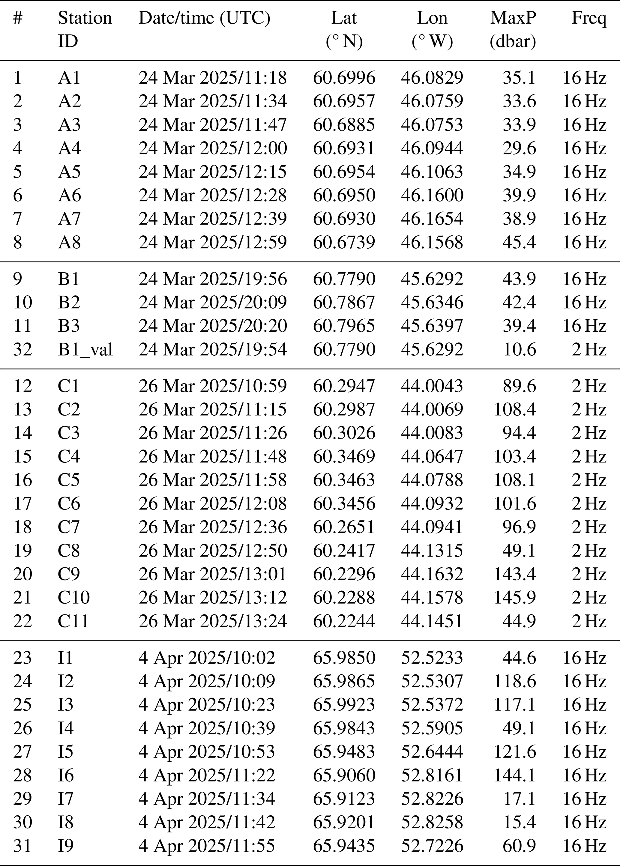
Table A2 FANS profile metadata (cruise CC170425, April 2025). Longitude in ° W. Profiles without GPS are indicated by –. MaxP: maximum valid sea pressure. Freq: sampling frequency.