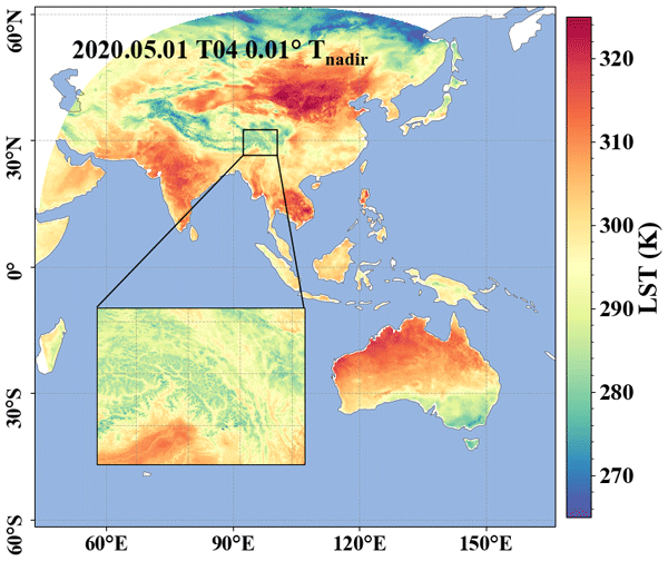
Generation of angular-normalized, cloud-filled, 0.01°-downscaled land surface temperature from 2018 to 2023 based on official FY-4A dataset

Land surface temperature (LST) is an essential climate variable in geophysical, ecological, and environmental research. Remote sensing provides a unique observation approach for obtaining large-scale LST products. However, current official LST datasets (such as FY-4A) are limited by the unaddressed thermal radiation directionality effect and suffer from the spatial discontinuities due to the pervasive presence of clouds. Moreover, geostationary LST products have relatively coarser resolution than those of polar-orbiting satellites due to trade-off between spatial and temporal resolutions. Based on the official hourly FY-4A LST dataset, this study proposes a novel framework for generating angular-normalized, cloud-filled, and 0.01°-downscaled LST (ANCFDS-LST) product, encompassing directional (T_dir), nadir (T_nadir), and hemispherical (T_hemi) LST layers. First, the angular-normalized T_nadir and T_hemi were generated using a time-evolving kernel driven model (TEKDM) with the inputs of multi-temporal FY-4A T_dir. Subsequently, hypothetical clear-sky LST was predicted using a CatBoost model optimized via Bayesian methods. The cloudy-sky LST values were then derived through a cloud radiation force (CRF) correction. Finally, the 0.05° all-weather T_dir, T_nadir, and T_hemi values were downscaled to 0.01° resolution using an improved hybrid downscaling algorithm (IHDA) combining kernel- and fusion-based methods. Taking the daytime clear-sky near-nadir VNP21A1 LST as reference, the 0.05° T_dir before angular-normalization has a root mean squared difference (RMSD) of 4.53 K and a mean bias difference (MBD) of −1.85 K, whereas the angularly normalized T_nadir has a much smaller RMSD of 2.56 K and a better MBD of 0.06 K. For the all-weather T_hemi, temperature-based validation over 8 sites in the Heihe River Basin and Australia shows a root mean squared error (RMSE) and mean bias error (MBE) of 2.48 and −0.83 K under clear-sky conditions, 3.65 and −1.43 K under cloudy-sky conditions. After the spatial downscaling, the 0.01° all-weather T_hemi exhibits abundant texture details. The generated LST products over the FY-4A disk from 2018 to 2023 exhibit enhanced angular consistency, spatial continuity, and finer resolution, offering valuable support for subsequent LST-related applications. The ANCFDS-LST data is freely available at https://doi.org/10.11888/RemoteSen.tpdc.303249 (Na et al., 2026).

1 Introduction

Land Surface Temperature (LST) quantifies the thermal properties of the Earth's land surface and serves as a driving force of climate change, radiation budgets, water cycle, and atmospheric processes (Wei et al., 2020, 2021). Compared to polar-orbiting satellite LST products, geostationary LSTs have the advantage of enhanced temporal resolution, which is more suitable to characterize the dynamic variations of land surface thermal conditions (Li et al., 2023c). To ensure both retrieval accuracy and computational efficiency, numerous easy-to-implement methods such as the split-window (SW) and temperature and emissivity separation (TES) methods have been developed for the geostationary satellites over the past decades (Li et al., 2013). These methods have been successfully applied in the generation of official LST products, including the Fengyun-4A (FY-4A) Advanced Geosynchronous Radiation Imager (AGRI) LST product (Dong et al., 2013, 2023a; Lin et al., 2025), Geostationary Operational Environmental Satellites R-Series (GOES-R) Advanced Baseline Imager (ABI) LST products (Yu et al., 2009), and the Meteosat Second Generation (MSG) Spinning Enhanced Visible and Infrared Imager (SEVIRI) LST product (Freitas et al., 2013; Trigo et al., 2011).

Despite the significant advancement of LST retrieval methods, current geostationary LST products still suffer from three major limitations: (1) most existing LST retrieval methods assume that surface-emitted radiance is isotropic. However, the complex structure and heterogeneous sub-pixel temperature distribution lead to different LST values when observing a pixel from different directions at the same time, i.e., the thermal radiation directionality (TRD) effect (Cao et al., 2019a). As a result, current LST products are directionally dependent and require normalization to a reference direction. (2) Because thermal-infrared (TIR) signals cannot penetrate clouds, current LST products exhibit significant spatial discontinuities, with more than half of the land surface often obscured by cloud cover (Stubenrauch et al., 2013). Therefore, generating all-weather (including clear-sky and cloudy-sky conditions) LST has attracted considerable research interest in the TIR remote sensing community (Jia et al., 2024; Wu et al., 2021). (3) A trade-off between spatial and temporal resolution is inherent to LST products. Hourly LST products from geostationary satellites typically have a spatial resolution of 2–5 km. Improving sensor performance is one direct approach, while spatial downscaling methods offer a more practical and efficient alternative for enhancing the texture detail of LST products (Sun et al., 2024; Wu et al., 2021; Zhan et al., 2013).

The influence of TRD effect during summer is as large as 4.0 K in sparsely vegetated areas and 5.1 K in urban regions (Coll et al., 2019; Du et al., 2023, 2025; Zhan et al., 2025). The semi-physical kernel-driven model (KDM) is regarded as the most promising approach for reducing LST angular dependence and achieving angular normalization (Cao et al., 2019b, 2021; Michel et al., 2023). It simulates the LST angular distribution through a linear combination of several kernel functions. The primary step is to calibrate the kernel coefficients, which then allows for correcting the directional LST (i.e., T_dir) to a nadir LST (i.e., T_nadir) or to a hemispherical LST (i.e., T_hemi) by integrating over the upper hemisphere. Solving for three or four unknown kernel coefficients typically requires at least three or four simultaneous multi-angle observations which cannot be satisfied by current satellite sensors. To address this problem, previous studies have either omitted one anisotropic kernel (Qin et al., 2023; Teng et al., 2023) or assumed that certain kernel coefficients remain constant over broad spatial or temporal scales (Chang et al., 2025; Ermida et al., 2017, 2018a, b; Vinnikov et al., 2012). Recently, Qin et al. (2025) proposed a time-evolving kernel-driven model (TEKDM) with seven parameters which captures the multi-temporal multi-angle LST patterns within a single day and enables the coefficient calibration in the overlapping region of two geostationary satellites. To broaden the application region of TEKDM, Na et al. (2024b) normalized the LST in the overlapping region of TERRA/AQUA Moderate Resolution Imaging Spectroradiometer (MODIS) and GOES-16 ABI LST products. Results showed that the root mean squared error (RMSE) was reduced from 3.29 to 2.34 K. Although angular normalization methods have been well developed, their large-scale application, validation, and the generation of operational nadir and hemispherical LST products remain unsolved, which has long been a key objective in the TIR remote sensing field. Here, the FY-4A AGRI and TERRA/AQUA MODIS official LST products were jointly employed for solving the TEKDM and achieving the angular normalization of FY-4A LST (i.e., producing T_nadir and T_hemi).

Due to the lack of TIR information of the land surface under cloudy-sky conditions, all-weather LST estimation for geostationary satellites typically relies on various types of auxiliary data and can be categorized into three main approaches: interpolation-based methods, surface energy balance (SEB) based methods, and simulation-based methods. Interpolation-based methods utilize spatially or temporally adjacent information to estimate missing LST values (Hong et al., 2021, 2022; Quan et al., 2018; Wang et al., 2024b). These methods can effectively preserve fine spatial textures, but they are uncertain under extensive cloud cover (Jia et al., 2024). Furthermore, they do not account for the influence of cloud radiation force (CRF). The SEB-based methods are commonly used to calculate the CRF effects in all-weather LST estimation. For example, Jia et al. (2021) proposed an iterative CRF correction method, Liu et al. (2023) solved a quartic equation to perform CRF correction, and Zhang et al. (2024) developed an analytical CRF correction formula. LST values after CRF correction can represent the actual thermal properties of the land surface and are recommended for large-scale applications (Jia et al., 2024; Wu et al., 2021). Simulation-based methods also show excellent potential for estimating all-weather LST, but they suffer from coarse resolution and substantial biases in simulated LST (Ding et al., 2022; Dong et al., 2022). The rapid advancement of machine learning (ML) models offers promising opportunities to improve the all-weather LST estimation. Zhang et al. (2024) recently proposed a two-step gap-filling algorithm. In the first step, hypothetical LST values are estimated using an ML model with the input of reanalysis data. Then, an SEB-based CRF correction is applied to generate the all-weather LST. Results showed stable accuracy with the maximum RMSE within 4 K. Physically, the clear-sky LST in SEB calculation should represent an integrated quantity over the upper hemisphere, which cannot be satisfied by current LST products (Jia et al., 2024). Instead, existing gap-filling methods typically rely on clear-sky directional LST (i.e., T_dir), thereby accumulating uncertainties associated with the TRD effect. In this study, Zhang's method is employed as the basic gap-filling framework. The angular independent clear-sky nadir and hemispherical LST (i.e., T_nadir, T_hemi) were introduced to improve the reliability of hypothetical LST and further enhance the accuracy of generated cloudy-sky LST.

Downscaling methods are widely used to produce LST products with high spatial resolution. These methods can generally be classified into three categories: kernel-based approaches (Dong et al., 2020; Zhan et al., 2013; Zhang et al., 2020; Zheng et al., 2024), fusion-based approaches (Tang et al., 2024; Wang et al., 2024b), and hybrid downscaling method combining both kernel- and fusion-based approaches (Dong et al., 2023b; Li et al., 2023b; Xia et al., 2019). Kernel-based methods typically establish a relationship between LST and regression kernels such as the normalized vegetation index (NDVI) at a coarse resolution. This relationship is then applied at a finer scale to generate high-resolution LST. These methods have evolved from simple linear regressions using single variables to ML-based regressions incorporating multiple kernels (Agam et al., 2007; Ebrahimy and Azadbakht, 2019; Xu et al., 2024; Zheng et al., 2024). Fusion-based methods aim to estimate fine-scale LST variability using multi-resolution LST data as inputs (Tang et al., 2024; Wang et al., 2024b; Wu et al., 2015). In these approaches, high-resolution LST temporal variation is typically estimated by weighting the coarse-resolution LST temporal variation of neighbouring similar pixels. The estimated temporal variation is then added to the high-resolution LST at the initial time to derive the final LST at the target time. A hybrid downscaling method combining both kernel- and fusion-based approaches offers improved accuracy and computational efficiency than single method (Dong et al., 2023b), which was adopted in this study. However, this method requires gap-free, high-resolution LST at the initial time as input, which is difficult to obtain at the full-disk scale due to the widespread presence of clouds over large areas. The annual temperature cycle (ATC) model has the potential to provide the necessary gap-free high-resolution LST texture information (Quan et al., 2018; Zhan et al., 2016) and thereby ensure the generation of 0.01° LST at the full-disk scale. Therefore, ATC-derived texture information was incorporated to extend and refine the hybrid downscaling method over a broader spatial extent.

It should be noted that this study does not aim to introduce incremental improvements to individual components, as the angular normalization, cloudy-sky reconstruction, and spatial downscaling modules have been previously developed. Instead, the novelty lies in establishing a unified processing framework that explicitly resolves angular inconsistency and enables their synergistic integration toward a conceptually consistent LST. By doing so, this work moves beyond conventional LST product generation and represents a step toward next-generation LST datasets that simultaneously satisfy the requirements of Global Climate Observing System (GCOS, https://gcos.wmo.int/site/global-climate-observing-system-gcos/essential-climate-variables/land-surface-temperature, last access: 16 June 2026), including ∼1 km spatial resolution, sub-daily temporal frequency, and climate-level consistency. The generation of hourly, angular-normalized, cloud-filled, and 0.01°-downscaled LST (ANCFDS-LST) consists of the following key steps: First, the TEKDM was calibrated using FY-4A and MODIS official LST products to generate daytime nadir and hemispherical LST at a 0.05° resolution. Second, an ML-based model was trained to generate hypothetical clear-sky LST, using angular-normalized LST as labels. Then, the all-weather LST was produced through an analytical CRF correction process. Finally, an improved hybrid downscaling algorithm (IHDA) combining kernel- and fusion-based methods was developed and carried out with the input of ATC-simulated gap-free 0.01° LST for producing the 0.01° all-weather directional, nadir, and hemispherical LST products. The hemispherical LST is validated using 8 sites in the Heihe River Basin and Australia, which measure the hemispherical longwave radiation via in situ pyrgeometer. The nadir LST is cross-validated using Visible Infrared Imaging Radiometer Suite (VIIRS) near nadir LST. The structure of this study is as follows: Sect. 2 describes the remote sensing and reanalysis data, cross-validation data and in situ validation data. Section 3 presents the TEKDM-based angular normalization method, the all-weather LST estimation method, and the IHDA downscaling approach. Section 4 provides the results of the generated LST products. Section 5 presents the discussion and limitation of this study. Sections 6 and 7 introduce the data availability and the main conclusions, respectively.

2 Data

2.1 Input remote sensing and reanalysis data

Table 1 lists the information of the required 15 datasets for the three main steps in the generation of ANCFDS-LST (namely, LST angular normalization, all-weather LST estimation, and spatial downscaling). The LST dataset produced in this study spans the period from 2018 to 2023, covering the full operational phase of the FY-4A LST product (note that the official FY-4A LST product has not been generated since 4 March 2024, as it has been superseded by a subsequent operational satellite). First, FY-4A and MODIS directional LSTs (i.e., 2 datasets) were used to generate angular-normalized nadir LST (T_nadir) and hemispherical LST (T_hemi). Next, 10 remote sensing and reanalysis products were employed to drive the generation of hypothetical clear-sky LST and the application of CRF correction, for estimating all-weather T_dir, T_nadir, and T_hemi at a 0.05° spatial resolution. Finally, these three 0.05° all-weather LST products were downscaled using 0.01° regression kernels obtained from 3 datasets, including MYD11A1, GTOPO30 DEM, and ERA5 Land.

Table 1 The employed remote sensing and reanalysis dataset.

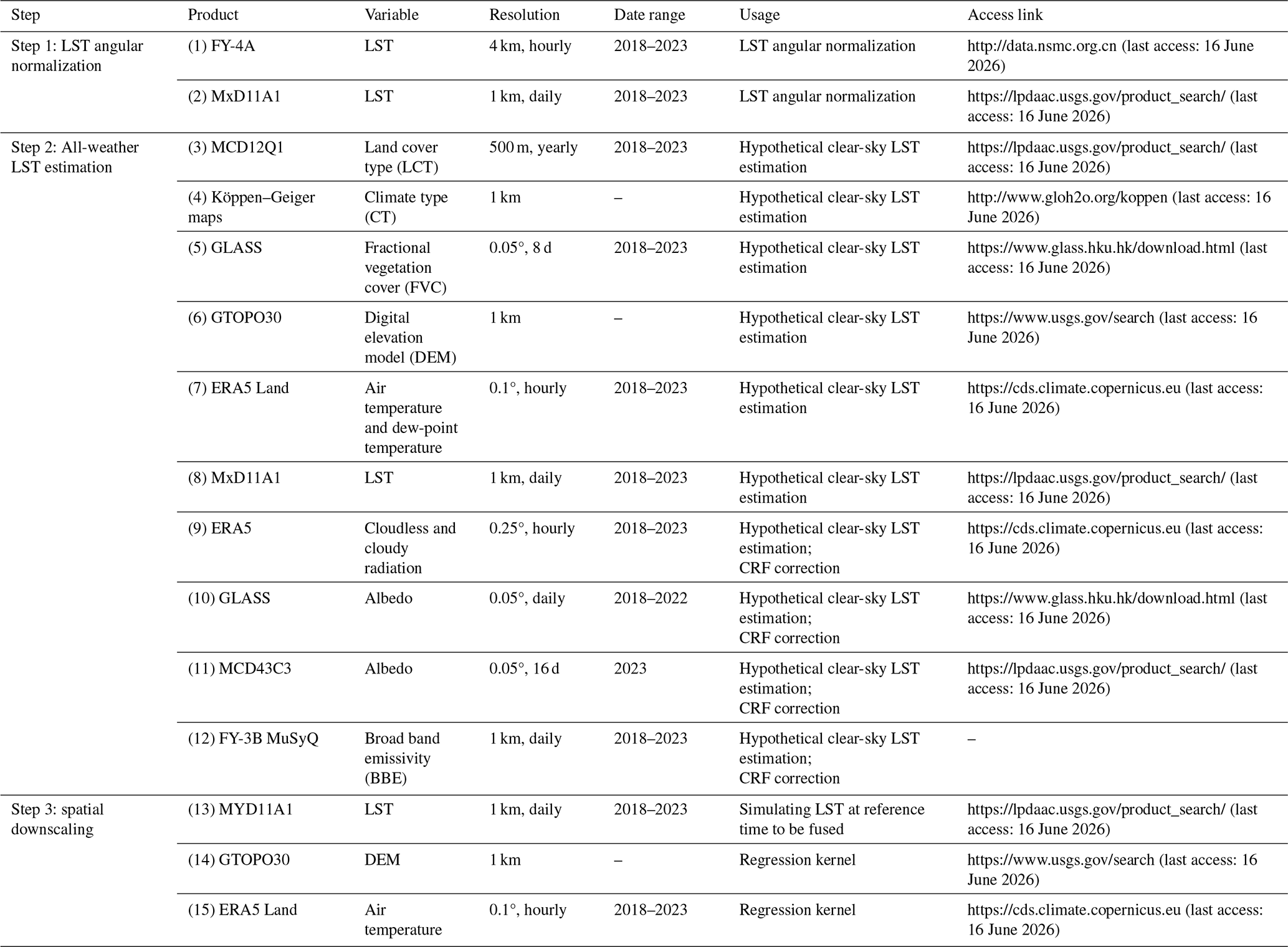
For the first step (i.e., LST angular normalization), the FY-4A directional LST (LST_FY) and MODIS LST (LST_MxD) products (i.e., datasets 1–2 in Table 1) were jointly utilized to calibrate the TEKDM model. Based on the calibrated model, clear-sky T_nadir and T_hemi were derived using the corresponding kernels and kernel coefficients. The official FY-4A LST is retrieved using a SW algorithm, with land surface emissivity (LSE) estimated via NDVI-based threshold method (Dong et al., 2013, 2023a). The MODIS MxD11A1 LST was retrieved using a generalized split-window (GSW) algorithm, incorporating land-cover-based LSE as input (Wan and Dozier, 1996). Both FY-4A and MODIS LST products were resampled to the same spatial resolution (i.e., 0.05°) using simple averaging before the joint estimation. Pixels with a view zenith angle (VZA) greater than 70° were masked (Freitas et al., 2013). To reduce systematic discrepancies between these two datasets, the 0.05° FY-4A LST was linearly adjusted to match the 0.05° MODIS MxD11A1 LST using a linear transformation (i.e., LST${}_{\mathrm{MxD}}=a\times {\mathrm{LST}}_{\mathrm{FY}}+b$). The parameters a and b were determined based on nighttime matchups under the condition of VZA < 50°, VZA difference < 5°, and LST difference < 5 K, referenced to Ermida et al. (2017, 2018a). A total of 132 972 698 matchup pairs were collected from 1 January 2018 to 31 December 2023 in the disk of FY-4A, resulting in a slope of a=1.0240 and an intercept of $b=-\mathrm{5.7378}$. It should be noted that all subsequent cloud-filling and downscaling procedures were performed based on the bias-corrected FY-4A LST, and thus the final released products are provided on the MODIS-referenced LST scale.

The second step (i.e., all-weather LST estimation) includes the estimation of hypothetical clear-sky LST and the CRF correction. In the hypothetical clear-sky LST estimation, datasets 3–7 in Table 1 – including the MCD12Q1 IGBP land cover type (LCT) product (dataset 3), the Köppen-Geiger climate type (CT) product (dataset 4), the Global LAnd Surface Satellite (GLASS) fractional vegetation cover (FVC) product (dataset 5), the GTOPO30 DEM data (dataset 6), the ERA5-Land 2 m air temperature (T_2 m), and dew-point temperature (D_2 m) data (dataset 7) – were employed to characterize surface properties (Wei et al., 2019). Moreover, datasets 8–12 in Table 1 were further used to calculate three additional variables to depict surface thermal conditions – including the ATC-simulated LST, the surface incoming radiation (R_in), and hypothetical clear-sky skin temperature (T_ERA5-skin).

The ATC model has three parameters as shown in Eq. (1), which was calibrated using the MxD11A1 LST product as input (dataset 8). In total, four ATC models were obtained since TERRA and AQUA MODIS sensors provide observations during both day and night. A 3×3 spatial median filter was applied to fill invalid ATC parameters caused by persistent cloud coverage. Then, the LST values simulated using the calibrated ATC model were used in the estimation of hypothetical clear-sky LST. These ATC-simulated LSTs are denoted as $T_{\mathrm{ATC},{\mathrm{d}}_{\mathrm{1}}}$, $T_{\mathrm{ATC},{\mathrm{d}}_{\mathrm{2}}}$, $T_{\mathrm{ATC},{\mathrm{n}}_{\mathrm{1}}}$, and $T_{\mathrm{ATC},{\mathrm{n}}_{\mathrm{2}}}$, where the subscripts “d” and “n” refer to daytime and nighttime data, respectively, and “1” and “2” indicate TERRA and AQUA platforms.

$$\begin{array}{}\text{(1)}& T_{\mathrm{ATC}}\left(\mathrm{DOY}\right)=\mathrm{MAST}+\mathrm{YAST}\times \cos \left[{\displaystyle \frac{\mathrm{2}\mathit{\pi }}{\mathrm{365}}}(\mathrm{DOY}-\mathrm{d}x)\right]\end{array}$$

where T_ATC(DOY) is the ATC-simulated LST as a function of day-of-year (DOY). MAST is the annual mean surface temperature, YAST is the yearly temperature amplitude, and dx is the phase shift. The QC band was filtered to ensure high-quality inputs for the ATC model calibration.

R_in is the sum of absorbed shortwave and longwave radiation as calculated in Eq. (2), with the input of surface downward shortwave radiation (SDSR_clr), land surface albedo (Albedo), surface downward longwave radiation (SDLR_clr) and broad band emissivity (BBE, ε_bb). Both SDSR_clr and SDLR_clr under hypothetical clear-sky condition are extracted from ERA5 products (dataset 9). The Albedo is from the GLASS product for 2018–2022 (dataset 10) and supplemented by MCD43C3 for 2023 (dataset 11). A Harmonic ANalysis of Time Series (HANTS) method was employed to smooth and fill the gaps in MCD43C3 product in this study (Zhou et al., 2022, 2023). The BBE is generated from MUlti-source data SYnergized Quantitative (MuSyQ) remote sensing system (dataset 12) (Li et al., 2019). Datasets 9–12 were resampled to a 0.05° resolution to match LST_FY.

$$\begin{array}{}\text{(2)}& R_{\mathrm{in}}=(\mathrm{1}-\mathrm{Albedo})\cdot {\mathrm{SDSR}}_{\mathrm{clr}}+{\mathit{\epsilon }}_{\mathrm{bb}}\cdot {\mathrm{SDLR}}_{\mathrm{clr}}\end{array}$$

Based on the Stefan–Boltzmann law, the ERA5 hypothetical clear-sky surface thermal radiation – e.g., surface downward longwave radiation (SDLR_clr) and surface net thermal radiation STR_clr – could be used to calculate the hypothetical clear-sky skin temperature (T_ERA5-skin) at a spatial resolution of 0.25° to depict temporal dynamics of LST. It was then physically downscaled to a 0.05° resolution using DEM data, assuming a temperature lapse rate (K) of 6.5 K km⁻¹ (Minder et al., 2010). Therefore, the T_ERA5-skin was calculated by the following equation:

$$\begin{array}{}\text{(3)}& \begin{array}{rl}{T}_{\mathrm{ERA}\mathrm{5}\text{-}\mathrm{skin}}& =\sqrt[\mathrm{4}]{{\displaystyle \frac{{\mathrm{SDLR}}_{\mathrm{clr}}-{\mathrm{STR}}_{\mathrm{clr}}-\left(\mathrm{1}-{\mathit{\epsilon }}_{\mathrm{bb}}\right){\mathrm{SDLR}}_{\mathrm{clr}}}{{\mathit{\epsilon }}_{\mathrm{bb}}{\mathit{\sigma }}_{\mathrm{s}}}}}\\ & +K\cdot \left({\mathrm{DEM}}_i-{\mathrm{DEM}}_m\right)\end{array}\end{array}$$

where σ_s is the Stefan–Boltzmann constant $\mathrm{5.67}\times {\mathrm{10}}^{-\mathrm{8}}$. The DEM_i and DEM_m refer to the elevation of the 0.05° pixel and the mean elevation of the corresponding 0.25° pixel, respectively.

After generating the hypothetical clear-sky LST, a CRF correction is required to convert it into cloudy-sky LST. This correction is physically based on the surface energy balance differences between clear-sky and cloudy conditions. Specifically, cloud-free and cloudy SDSR from ERA5 reanalysis data (dataset 9), together with albedo data (dataset 10 and 11), are used to describe the shortwave radiation budget. For the longwave radiation budget, ERA5 cloud-free and cloudy-sky SDLR data (dataset 9), BBE data (dataset 12), the hypothetical clear-sky LST and cloudy-sky LST are required. Then, the only unknown variable, cloudy-sky LST (expressed as the sum of hypothetical clear-sky LST and the CRF correction value) can be retrieved by solving the SEB equation. More details will be given in Sect. 3.2.

In the third step (i.e., spatial downscaling), a new algorithm combining existing kernel- and fusion-based methods was proposed to downscale LST to the target time, consisting of two main processes. First, a 0.05° gap-free high-resolution LST at the initial time is required. In this study, $T_{\mathrm{ATC},{\mathrm{d}}_{\mathrm{2}}}$ simulated by the ATC model (dataset 13) is resampled as the initial LST. Second, the 0.05° LST difference between the initial and target time is predicted using an ML method. The input features include $T_{\mathrm{ATC},{\mathrm{d}}_{\mathrm{2}}}$; AQUA MODIS ATC parameters for both day (MAST${}_{{\mathrm{d}}_{\mathrm{2}}}$, YAST${}_{{\mathrm{d}}_{\mathrm{2}}}$, and $\mathrm{d}{x}_{{\mathrm{d}}_{\mathrm{2}}}$) and night (MAST${}_{{\mathrm{n}}_{\mathrm{2}}}$, YAST${}_{{\mathrm{n}}_{\mathrm{2}}}$, and $\mathrm{d}{x}_{{\mathrm{n}}_{\mathrm{2}}}$), derived from dataset 13; DEM data (dataset 14); and ERA5-Land T_2 m (dataset 15). To apply this spatial downscaling model at the 0.01° scale, the T_2 m data were further downscaled to 0.01° resolution using high-resolution DEM and the temperature lapse rate (K) of 6.5 K km⁻¹. Finally, the gap-free high-resolution LST at the target time is obtained by adding the estimated 0.01° LST difference to 0.01° $T_{\mathrm{ATC},{\mathrm{d}}_{\mathrm{2}}}$.

2.2 Cross-validation dataset for T_nadir

For cross-validation of the generated T_nadir, the VIIRS VNP21A1 LST data (https://lpdaac.usgs.gov/product_search/, last access: 16 June 2026) in 2020 was adopted as reference. The VIIRS instrument onboard the Suomi National Polar-orbiting Partnership (S-NPP) satellite provides clear-sky TIR observations at 13:30 LT (local time). The VNP21 LST was retrieved using a TES algorithm using observations from the M14–M16 bands as input. Recent temperature-based (T-based) evaluation showed that its RMSE is 1.79 K during nighttime and 2.79 K during the day (Na et al., 2024a). Here, VNP21 LST values with the VZA < 5° were employed for cross-evaluation of T_nadir as done by Wei et al. (2025). Meanwhile, the MODIS-referenced FY-4A LST product was temporally interpolated to match the exact observation time of VIIRS LST. The resulting near-nadir VNP21 LST was first resampled to a spatial resolution of 0.05°, and then bias-corrected to MODIS-referenced FY-4A LST using nighttime matchups (consistent with the bias correction applied between MODIS and FY-4A LST products). A total of 12 379 672 matchup pairs were collected over the full disk of FY-4A in 2020, yielding a regression slope of 0.9478 and an intercept of 13.9510. This relationship was subsequently applied to the daytime VIIRS near-nadir LST. After bias correction, the root mean square difference (RMSD) between the VIIRS LST and MODIS-referenced FY-4A LST decreased from 6.21 to 4.53 K, while the mean bias difference (MBD) was reduced from −4.04 to −1.85 K. Finally, the RMSD, MBD, and coefficient of determination (R²) were used as three evaluation indicators for the cross-validation. The extracted VNP21 LST results for four typical days are shown in Fig. 1. Only several narrow strips were extracted due to the limitation of VIIRS field-of-view (VZA < 5°). VNP21 LST shows significant seasonal variation. It is relatively lower in 1 March and 1 December 2020 than that in 1 June and 1 September 2020 in the northern hemisphere and the situation is reversed in the southern hemisphere.

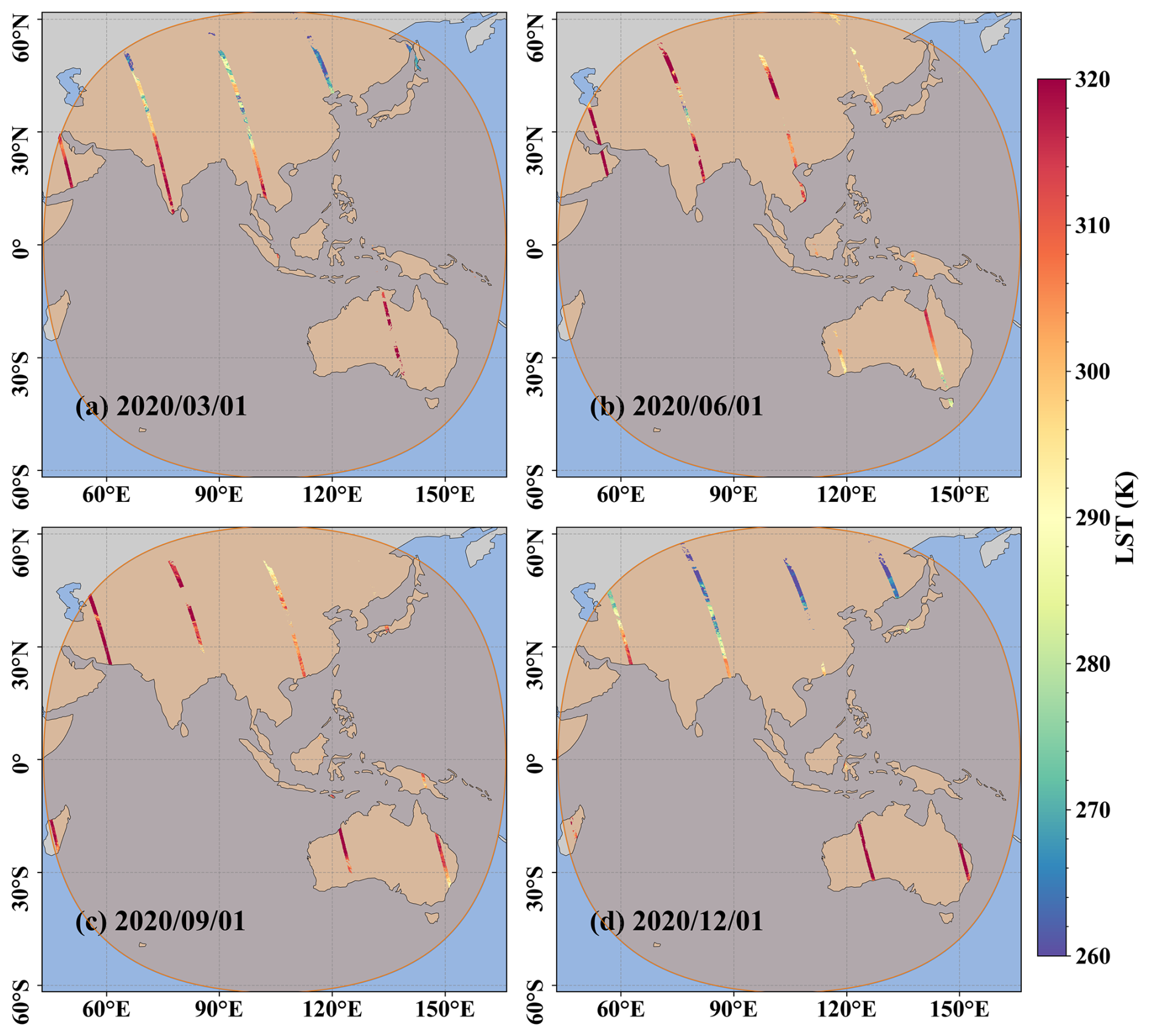
Figure 1 Spatial distribution of the extracted VNP21 LST strips in four typical days (a) 1 March 2020, (b) 1 June 2020, (c) 1 September 2020, (d) 1 December 2020. The FY-4A observed area is marked in the orange region.

2.3 In situ validation dataset for T_hemi

T-based evaluation (i.e., directly comparing satellite-derived LST with in situ LST) is the most widely used validation method and should be performed whenever possible (Guillevic et al., 2018; Li et al., 2014, 2023a; Na et al., 2024a). The in situ pyrgeometer measures both upward and downward hemispherical longwave radiation, which can be converted into hemispherical LST to perform the T-based validation for the normalized T_hemi products. As shown in Fig. 2, 5 sites from the Heihe Watershed Allied Telemetry Experimental Research (HiWATER) experiment within the Heihe River Basin (HRB) and 3 sites from the Terrestrial Ecosystem Research Network (TERN) OzFlux network in 2020 were selected, which have been used in LST evaluation studies (Beringer et al., 2016; Che et al., 2019; Li et al., 2025, 2020). More detailed information on the in situ sites is listed in Table 2. In addition, the median standard deviation (SD) of Landsat 8 LST within a 0.05° window and the RMSE between nighttime FY-4A LST and in situ LST are also provided, as these two metrics were used to assess the spatial representativeness of the selected validation sites (see Sect. 5.3).

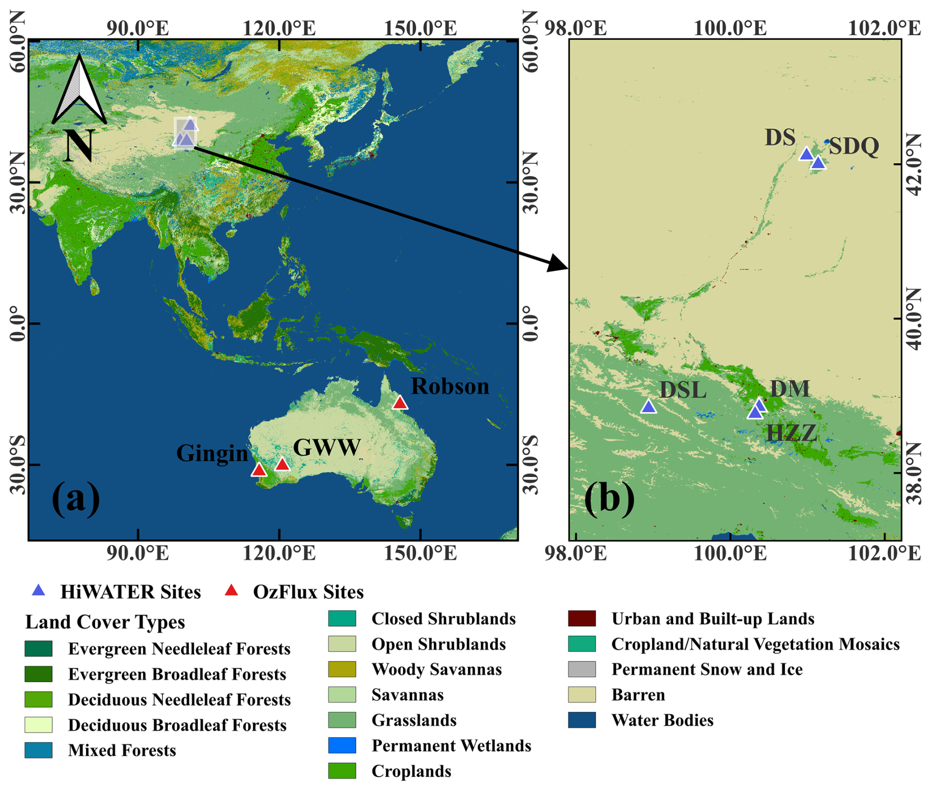
Figure 2 Spatial distribution of selected in situ sites.

Table 2 Information of the in situ sites.

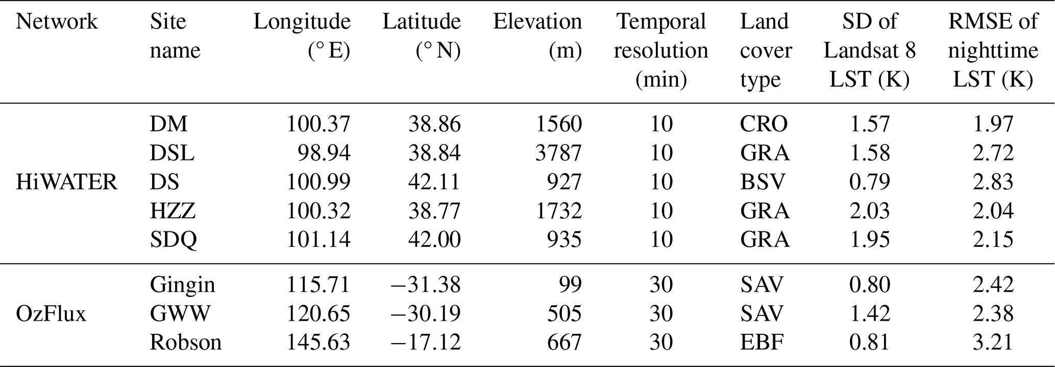
As listed in Table 2, five land cover types are represented across the 8 validation sites: 1 cropland (CRO) site, 3 grassland (GRA) sites, 1 barren/sparse vegetation (BSV) site, 2 savanna (SAV) sites, and 1 evergreen broadleaf forest (EBF) site. The temporal resolution of the in situ observations varies by network: 10 min for the HiWATER sites, and 30 min for the OzFlux sites. Linear interpolation was applied to align in situ measurements with the exact satellite observation time. The in situ LST (T_insitu) is calculated using the Stefan–Boltzmann law, as shown in Eq. (4):

$$\begin{array}{}\text{(4)}& T_{\mathrm{insitu}}=\sqrt[\mathrm{4}]{{\displaystyle \frac{{\mathrm{SULR}}_{\mathrm{insitu}}-\left(\mathrm{1}-{\mathit{\epsilon }}_{\mathrm{bb}}\right){\mathrm{SDLR}}_{\mathrm{insitu}}}{{\mathit{\epsilon }}_{\mathrm{bb}}{\mathit{\sigma }}_{\mathrm{s}}}}}\end{array}$$

where SULR_insitu and SDLR_insitu are the surface upward and downward longwave radiation measured by the in situ pyrgeometer, respectively. ε_bb is the broadband emissivity derived from the FY-3B MuSyQ product. Outliers were identified and removed using the “3σ-Hampel identifier” method for each site (Davies and Gather, 1993; Pearson, 2002). The RMSE, mean bias error (MBE), and R² were used as evaluation metrics to validate the LST products.

3 Method

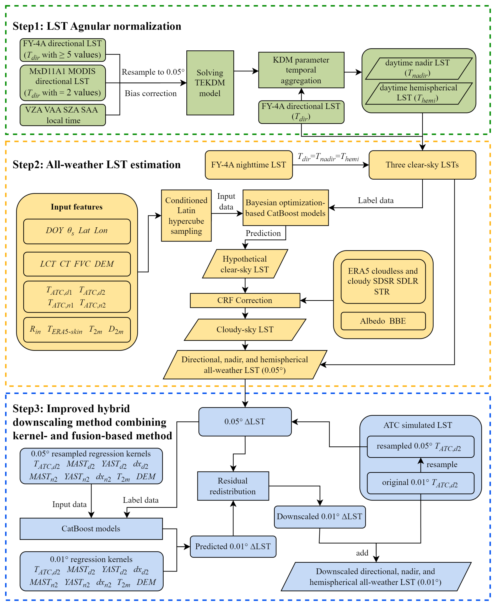
The generation of 0.01° ANCFDS-LST involves three main steps: (1) angular normalization of daytime LST; (2) generation of 0.05° all-weather LST using clear-sky LST as labels; (3) downscaling of all-weather LST to 0.01° resolution using an IHDA method. The overall flowchart is shown in Fig. 3. First, 0.05° clear-sky FY-4A and resampled MxD11A1 directional LST products were matched and bias corrected for solving the unknown parameters of TEKDM using auxiliary information of viewing geometry and local time. For the generation of T_nadir and T_hemi from FY-4A T_dir, the KDM coefficients were temporally aggregated over a 17 d window to ensure a complete spatial coverage of the FY-4A disk. Second, clear-sky T_dir, T_nadir, and T_hemi during the day, as well as nighttime FY-4A LST (where $T_{\mathrm{dir}}=T_{\mathrm{nadir}}=T_{\mathrm{hemi}}$ due to the negligible angular effect at night) were used as training labels to predict the hypothetical clear-sky LST under cloudy conditions. A Bayesian optimization-based categorical boosting (CatBoost) model was trained using auxiliary input variables described in Sect. 2.1. The training samples were spatially determined using a widely used conditioned Latin hypercube sampling (cLHS) approach. The predicted hypothetical clear-sky LST requires a CRF correction using the cloudless and cloudy radiation budget variables, ultimately yielding the cloudy-sky T_dir, T_nadir, and T_hemi. In the third step, the 0.05° all-weather LST was downscaled to 0.01° resolution using a proposed IHDA method. This approach downscales the LST difference (ΔLST) between the 0.05° all-weather LST and the 0.05° $T_{\mathrm{ATC},{\mathrm{d}}_{\mathrm{2}}}$ at the reference time (i.e., 13:30 LT) using another CatBoost model. After predicting three ΔLSTs at 0.01° resolution and applying a residual redistribution procedure, the final downscaled 0.01° ΔLSTs were obtained. The final 0.01° all-weather T_dir, T_nadir, and T_hemi were derived by summing the corresponding downscaled 0.01° ΔLST with the corresponding 0.01° ATC-simulated LST.

Figure 3 The overall workflow in this study.

3.1 Angular normalization of clear-sky LST

The FY-4A LST disk has different viewing geometries for each pixel, and these values need to be normalized to a reference direction before subsequent applications. The KDM offers a solution by simulating the angular distribution of LST through a linear combination of several kernel functions. However, traditional KDM typically requires three or four simultaneous clear-sky LST observations to calibrate the unknown kernel coefficients, which cannot be satisfied by FY-4A satellite. To enhance its applicability, Qin et al. (2023, 2025) proposed a time-evolving KDM (TEKDM) by coupling a diurnal temperature cycle (DTC) model (i.e., depicting LST temporal variation) and a KDM model (i.e., depicting LST angular variation) as shown in Eq. (5). Based on this TEKDM model, Na et al. (2024b) further estimated daytime nadir LST using GOES-16 and MODIS LST products, and obtained a significantly improved accuracy.

$$\begin{array}{}\text{(5)}& \begin{array}{rl}{T}_{\mathrm{dir}}\left(t,{\mathit{\theta }}_{\mathrm{s}},{\mathit{\theta }}_{\mathrm{v}},\mathrm{\Delta }\mathit{\phi }\right)& =f_{\mathrm{iso}}\left(t\right)\times \left[\mathrm{1}+\mathit{\alpha }\cdot K_{\mathrm{GapFraction}}\left({\mathit{\theta }}_{\mathrm{v}}\right)\right.\\ & \left.+\mathit{\beta }\cdot \cos {\mathit{\theta }}_{\mathrm{s}}\cdot K_{\mathrm{Hotspot}}\left({\mathit{\theta }}_{\mathrm{s}},{\mathit{\theta }}_{\mathrm{v}},\mathrm{\Delta }\mathit{\phi },W\right)\right]\end{array}\end{array}$$

where $T_{\mathrm{dir}}(t,{\mathit{\theta }}_{\mathrm{s}},{\mathit{\theta }}_{\mathrm{v}},\mathrm{\Delta }\mathit{\phi })$ represents the directional LST observed at the local time of t, with the solar zenith angle (SZA) of θ_s, the VZA of θ_v, and the relative azimuth angle (RAA) of Δφ. The term f_iso(t) is the isotropic kernel coefficient. The coefficients α and β are unknowns corresponding to the gap fraction kernel (K_GapFraction) and hotspot kernel (K_Hotspot), respectively. W is another unknown parameter related to the hotspot width. The temporal dynamics of isotropic kernel coefficient (i.e., f_iso(t)) during daytime can be effectively modeled using a DTC model as given in Eq. (6):

$$\begin{array}{}\text{(6)}& f_{\mathrm{iso}}\left(t\right)=T_{\mathrm{0}}+T_{\mathrm{a}}\times \cos \left[{\displaystyle \frac{\mathit{\pi }}{\mathit{\omega }}}\cdot \left(t-t_{\mathrm{m}}\right)\right]\end{array}$$

where T₀ is the temperature at sunrise, T_a represents the amplitude of daily LST variation, ω is the length of the daytime period, t_m is the local time at which the LST reaches its maximum. The nighttime LST was not processed here, as the angular effect is generally negligible during nighttime. In this study, the LSF kernel and the Chen kernel were selected to represent K_GapFraction and K_Hotspot respectively, as shown in Eqs. (7)–(9).

$$\begin{array}{}\text{(7)}& {\displaystyle }\begin{array}{rl}{K}_{\mathrm{GapFraction}}\left({\mathit{\theta }}_{\mathrm{v}}\right)& =K_{\mathrm{LSF}}\left({\mathit{\theta }}_{\mathrm{v}}\right)={\displaystyle \frac{\mathrm{1}+\mathrm{2}\cos {\mathit{\theta }}_{\mathrm{v}}}{\sqrt{\mathrm{0.96}}+\mathrm{1.92}\cos {\mathit{\theta }}_{\mathrm{v}}}}\\ & -{\displaystyle \frac{\mathrm{1}}{\mathrm{4}}}\cdot {\displaystyle \frac{\cos {\mathit{\theta }}_{\mathrm{v}}}{\mathrm{1}+\mathrm{2}\cos {\mathit{\theta }}_{\mathrm{v}}}}+\mathrm{0.15}\cdot \left(\mathrm{1}-e^{\frac{-\mathrm{0.75}}{\cos {\mathit{\theta }}_{\mathrm{v}}}}\right)\\ & -\mathrm{1.0304}\end{array}\text{(8)}& {\displaystyle }{K}_{\mathrm{Hotspot}}\left({\mathit{\theta }}_{\mathrm{s}},{\mathit{\theta }}_{\mathrm{v}},\mathrm{\Delta }\mathit{\phi },W\right)=K_{\mathrm{Chen}}\left({\mathit{\theta }}_{\mathrm{s}},{\mathit{\theta }}_{\mathrm{v}},\mathrm{\Delta }\mathit{\phi },W\right)=e^{\frac{-\mathit{\xi }}{\mathit{\pi }\cdot W}}\text{(9)}& {\displaystyle }\mathit{\xi }=\arccos \left(\cos {\mathit{\theta }}_{\mathrm{v}}\cdot \cos {\mathit{\theta }}_{\mathrm{s}}+\sin {\mathit{\theta }}_{\mathrm{v}}\cdot \sin {\mathit{\theta }}_{\mathrm{s}}\cdot \cos \mathrm{\Delta }\mathit{\phi }\right)\end{array}$$

where ξ is the angular distance between the viewing direction and the solar direction. The TEKDM involves seven unknown parameters to be calibrated: T₀, T_a, ω, t_m, α, β, and W, therefore, at least seven clear-sky daytime observations are required as inputs. To enhance the angular information content of the input data, two daytime clear-sky MODIS observations (i.e., TERRA and AQUA) were utilized. Then, the TEKDM can be solved under the condition with ≥5 clear-sky FY-4A observations. A “trust-region-reflective” algorithm was employed for the non-linear optimization of Eq. (5), with initial values and parameter boundaries set according to Qin et al. (2025). Then, a 17 d moving average (i.e., covering 8 d before and after the target day) was applied to the parameters of α, β, and W for each pixel for two purposes: filling gaps in pixels with fewer than seven observations, and reducing the impact of outliers in the estimated TEKDM parameters. As shown in Eq. (10), the LST at any direction (i.e., the $T_{\mathrm{dir}}(t,{\mathit{\theta }}_{\mathrm{s}},{\mathit{\theta }}_{\mathrm{v}},\mathrm{\Delta }\mathit{\phi })$) can be simulated with the input of FY-4A direction LST – i.e., $T_{\mathrm{dir}}(t,{\mathit{\theta }}_{\mathrm{s}},{\mathit{\theta }}_{\mathrm{v}}^{\mathrm{FY}},\mathrm{\Delta }{\mathit{\phi }}^{\mathrm{FY}})$ – and averaged α, β, and W parameters.

$$\begin{array}{}\text{(10)}& \begin{array}{rl}& {\displaystyle \frac{T_{\mathrm{dir}}\left(t,{\mathit{\theta }}_{\mathrm{s}},{\mathit{\theta }}_{\mathrm{v}},\mathrm{\Delta }\mathit{\phi }\right)}{T_{\mathrm{dir}}\left(t,{\mathit{\theta }}_{\mathrm{s}},{\mathit{\theta }}_{\mathrm{v}}^{\mathrm{FY}},\mathrm{\Delta }{\mathit{\phi }}^{\mathrm{FY}}\right)}}=\\ & {\displaystyle \frac{\mathrm{1}+\mathit{\alpha }\cdot K_{\mathrm{LSF}}\left({\mathit{\theta }}_{\mathrm{v}}\right)+\mathit{\beta }\cdot \cos {\mathit{\theta }}_{\mathrm{s}}\cdot K_{\mathrm{Chen}}\left({\mathit{\theta }}_{\mathrm{s}},{\mathit{\theta }}_{\mathrm{v}},\mathrm{\Delta }\mathit{\phi },W\right)}{\mathrm{1}+\mathit{\alpha }\cdot K_{\mathrm{LSF}}\left({\mathit{\theta }}_{\mathrm{v}}^{\mathrm{FY}}\right)+\mathit{\beta }\cdot \cos {\mathit{\theta }}_{\mathrm{s}}\cdot K_{\mathrm{Chen}}\left({\mathit{\theta }}_{\mathrm{s}},{\mathit{\theta }}_{\mathrm{v}}^{\mathrm{FY}},\mathrm{\Delta }{\mathit{\phi }}^{\mathrm{FY}},W\right)}}\end{array}\end{array}$$

Specifically, the nadir LST can be derived when setting θ_v=0° as shown in Eq. (11):

$$\begin{array}{}\text{(11)}& \begin{array}{rl}& T_{\mathrm{nadir}}\left(t,{\mathit{\theta }}_{\mathrm{s}},\mathrm{0}\mathit{°},\mathrm{\Delta }\mathit{\phi }\right)=T_{\mathrm{dir}}\left(t,{\mathit{\theta }}_{\mathrm{s}},{\mathit{\theta }}_{\mathrm{v}}^{\mathrm{FY}},\mathrm{\Delta }{\mathit{\phi }}_{\mathrm{v}}^{\mathrm{FY}}\right)\\ & \cdot {\displaystyle \frac{\mathrm{1}+\mathit{\alpha }\cdot K_{\mathrm{LSF}}\left(\mathrm{0}\mathit{°}\right)+\mathit{\beta }\cdot \cos {\mathit{\theta }}_{\mathrm{s}}\cdot K_{\mathrm{Chen}}\left({\mathit{\theta }}_{\mathrm{s}},\mathrm{0}\mathit{°},\mathrm{\Delta }\mathit{\phi },W\right)}{\mathrm{1}+\mathit{\alpha }\cdot K_{\mathrm{LSF}}\left({\mathit{\theta }}_{\mathrm{v}}^{\mathrm{FY}}\right)+\mathit{\beta }\cdot \cos {\mathit{\theta }}_{\mathrm{s}}\cdot K_{\mathrm{Chen}}\left({\mathit{\theta }}_{\mathrm{s}},{\mathit{\theta }}_{\mathrm{v}}^{\mathrm{FY}},\mathrm{\Delta }{\mathit{\phi }}_{\mathrm{v}}^{\mathrm{FY}},W\right)}}.\end{array}\end{array}$$

Correspondingly, the normalized hemispherical LST (T_hemi) could be calculated through integration as shown in Eq. (12).

$$\begin{array}{}\text{(12)}& \begin{array}{rl}& T_{\mathrm{hemi}}\left(t,{\mathit{\theta }}_{\mathrm{s}}\right)={\left({\displaystyle \frac{\mathrm{1}}{\mathit{\pi }}}\cdot \underset{\mathrm{0}}{\overset{\mathrm{2}\mathit{\pi }}{\int }}\underset{\mathrm{0}}{\overset{\mathit{\pi }/\mathrm{2}}{\int }}{T}_{\mathrm{dir}}^{\mathrm{4}}\left(t,{\mathit{\theta }}_{\mathrm{s}},{\mathit{\theta }}_{\mathrm{v}},\mathrm{\Delta }\mathit{\phi }\right)\cdot \cos {\mathit{\theta }}_{\mathrm{v}}\cdot \sin {\mathit{\theta }}_{\mathrm{v}}\mathrm{d}{\mathit{\theta }}_{\mathrm{v}}\mathrm{d}{\mathit{\phi }}_{\mathrm{v}}\right)}^{\frac{\mathrm{1}}{\mathrm{4}}}\\ & ={\displaystyle \frac{T_{\mathrm{dir}}\left(t,{\mathit{\theta }}_{\mathrm{s}},{\mathit{\theta }}_{\mathrm{v}}^{\mathrm{FY}},\mathrm{\Delta }{\mathit{\phi }}_{\mathrm{v}}^{\mathrm{FY}}\right)\cdot {\left(\frac{\mathrm{1}}{\mathit{\pi }}\cdot \underset{\mathrm{0}}{\overset{\mathrm{2}\mathit{\pi }}{\int }}\underset{\mathrm{0}}{\overset{\mathit{\pi }/\mathrm{2}}{\int }}{\left(\mathrm{1}+\mathit{\alpha }\cdot K_{\mathrm{LSF}}\left({\mathit{\theta }}_{\mathrm{v}}\right)+\mathit{\beta }\cdot \cos {\mathit{\theta }}_{\mathrm{s}}\cdot K_{\mathrm{Chen}}\left({\mathit{\theta }}_{\mathrm{s}},{\mathit{\theta }}_{\mathrm{v}},\mathrm{\Delta }\mathit{\phi },W\right)\right)}^{\mathrm{4}}\cdot \cos {\mathit{\theta }}_{\mathrm{v}}\cdot \sin {\mathit{\theta }}_{\mathrm{v}}\mathrm{d}{\mathit{\theta }}_{\mathrm{v}}\mathrm{d}{\mathit{\phi }}_{\mathrm{v}}\right)}^{\frac{\mathrm{1}}{\mathrm{4}}}}{\left(\mathrm{1}+\mathit{\alpha }\cdot K_{\mathrm{LSF}}\left({\mathit{\theta }}_{\mathrm{v}}^{\mathrm{FY}}\right)+\mathit{\beta }\cdot \cos {\mathit{\theta }}_{\mathrm{s}}\cdot K_{\mathrm{Chen}}\left({\mathit{\theta }}_{\mathrm{s}},{\mathit{\theta }}_{\mathrm{v}}^{\mathrm{FY}},\mathrm{\Delta }{\mathit{\phi }}_{\mathrm{v}}^{\mathrm{FY}},W\right)\right)}}\end{array}\end{array}$$

To accelerate the computation of T_hemi, the integral in the numerator of Eq. (12) was approximated using a third-order polynomial fit based on the input variables of α, β, W, θ_s and K_Chen at nadir. More details about the integration procedure are provided in Appendix A. As shown in Fig. A1, this polynomial approximation substantially reduces computational cost while introducing an uncertainty of less than 0.1 K.

3.2 All-weather LST estimation method

The all-weather LST estimation method consists of two main sub-steps. First, a hypothetical clear-sky LST was predicted using a Bayesian optimization-based CatBoost model. Second, the CRF correction was applied to estimate the cloudy-sky LST, ultimately producing cloud-filled 0.05° all-weather directional, nadir, and hemispherical LST.

ML-based LST reconstruction methods have been widely used because they can accurately simulate the non-linear relationship between the hypothetical clear-sky LST and vegetative, meteorological, and topographical parameters (Li et al., 2024a; Ma et al., 2024a; Zhang et al., 2024). The CatBoost is a recently developed model based on the traditional gradient-boosting decision tree (GBDT) framework with several enhancements: (1) ordered target statistics, which encode categorical features without target leakage by using permutation-based strategies; (2) ordered boosting, which minimizes gradient bias by employing permutation-driven training to reduce overfitting; (3) oblivious trees, which apply the same splitting criterion across all nodes at each level, thereby improving speed and regularization (Prokhorenkova et al., 2018). These improvements enhance the model's robustness and efficiency, especially when handling large-scale datasets containing categorical variables, and have proven effective in LST reconstruction studies (Dai et al., 2025). Here, the CatBoost model was used to capture the complex non-linear relationship (i.e., f_clr) between hypothetical clear-sky LST and the auxiliary parameters, as represented in Eq. (13).

$$\begin{array}{}\text{(13)}& \begin{array}{rl}{T}_{\mathrm{clr}}=& f_{\mathrm{clr}}\left(\mathrm{DOY},{\mathit{\theta }}_{\mathrm{s}},\mathrm{Lat},\mathrm{Lon},\mathrm{LCT},\mathrm{CT},\mathrm{FVC},\mathrm{DEM},\right.\\ & T_{\mathrm{ATC},{\mathrm{d}}_{\mathrm{1}}},T_{\mathrm{ATC},{\mathrm{d}}_{\mathrm{2}}},T_{\mathrm{ATC},{\mathrm{n}}_{\mathrm{1}}},T_{\mathrm{ATC},{\mathrm{n}}_{\mathrm{2}}},R_{\mathrm{in}},\\ & \left.T_{\mathrm{ERA}\mathrm{5}\text{-}\mathrm{skin}},T_{\mathrm{2}\mathrm{m}},D_{\mathrm{2}\mathrm{m}}\right)\end{array}\end{array}$$

where the input features include the geolocation and temporal parameters, such as the DOY, θ_s, latitude (Lat), longitude (Lon). The other parameters in Eq. (13) have been introduced in Table 1. It should be noted that the reanalysis variables are introduced to provide spatial information that is not captured by satellite observations, rather than to replace satellite information. The primary observational constraint remains the official FY-4A LST products. The clear-sky LST values remain unchanged and also act as the training labels for cloudy-sky LST estimation.

The target labels consisted of daytime T_dir, T_nadir, and T_hemi, along with nighttime FY-4A LST from 1 January 2018 to 31 December 2023. A total of six ML models were trained on a year-by-year basis for each target temperature, rather than using a single model across multiple years. Each model is applied exclusively to data from its corresponding year, without temporal extrapolation to other periods. Considering the large volume of label data, a two-step approach was employed to determine the number and geolocation of sample points as introduced in Appendix B. As shown in Fig. B1, 37 000 locations distributed over the FY-4A disk were selected for each year. Then, the clear-sky LST and corresponding input features were extracted to train the CatBoost model in Eq. (13). To better align with the 0.25° spatial resolution of ERA5, a FY-4A pixel was strictly considered as clear-sky only when all surrounding pixels within a 5×5 neighbourhood were under clear-sky conditions. Six CatBoost models were trained for each year from 2018 to 2023. The average number of extracted samples per year was 138 817 085, which were randomly divided into training, testing, and Bayesian optimization sets in a ratio of $\mathrm{6}:\mathrm{3}:\mathrm{1}$. The Bayesian optimization method adjusted the CatBoost hyperparameters by reconstructing the posterior distribution of the cost function, defined as the average fitting RMSE from two-fold cross-validation. After the ML training, the CatBoost model can predict the hypothetical clear-sky T_dir, T_nadir, and T_hemi under cloudy-sky conditions, which requires CRF correction.

The core of the CRF correction lies in establishing the relationship between net radiation changes and CRF-induced LST changes, based on the surface radiation budget equation. The CRF-corrected LST is equal to the sum of hypothetical clear-sky LST with CRF-induced LST variation (i.e., ΔT_CRF). Considering that our aim is not to fully resolve the SEB equation, a simplified analytical correction equation (Eq. 14) proposed by Zhang et al. (2024) was adopted for the CRF correction of T_hemi.

$$\begin{array}{}\text{(14)}& \mathit{\gamma }\cdot \mathrm{\Delta }{T}_{\mathrm{CRF}}=\mathrm{\Delta }{R}_{\mathrm{in}}-{\mathit{\epsilon }}_{\mathrm{bb}}{\mathit{\sigma }}_{\mathrm{s}}\left[{\left(T_{\mathrm{clr}}^{\mathrm{hemi}}+\mathrm{\Delta }{T}_{\mathrm{CRF}}\right)}^{\mathrm{4}}-{\left(T_{\mathrm{clr}}^{\mathrm{hemi}}\right)}^{\mathrm{4}}\right]\end{array}$$

where ΔT_CRF is the correction value for hemispherical LST; γ is an energy transfer parameter, which could be estimated by Eq. (15). A temporal median filter with a 17 d window and a spatial median filter with a 3×3 window were applied to replace outlier values in the calculation of γ. ΔR_in is the change in surface incoming radiation induced by the CRF effect, which could be estimated by Eq. (16); $T_{\mathrm{clr}}^{\mathrm{hemi}}$ is predicted hypothetical clear-sky hemispherical LST using Eq. (13).

$$\begin{array}{}\text{(15)}& {\displaystyle }\mathit{\gamma }={\displaystyle \frac{\left[R_{\mathrm{in}}\left(t_{\mathrm{n}}\right)-R_{\mathrm{in}}\left(t_{\mathrm{sr}}\right)\right]-{\mathit{\epsilon }}_{\mathrm{bb}}{\mathit{\sigma }}_{\mathrm{s}}\left[T_{\mathrm{clr}}^{\mathrm{hemi}}{\left(t_{\mathrm{n}}\right)}^{\mathrm{4}}-T_{\mathrm{clr}}^{\mathrm{hemi}}{\left(t_{\mathrm{sr}}\right)}^{\mathrm{4}}\right]}{T_{\mathrm{clr}}^{\mathrm{hemi}}\left(t_{\mathrm{n}}\right)-T_{\mathrm{clr}}^{\mathrm{hemi}}\left(t_{\mathrm{sr}}\right)}}\text{(16)}& {\displaystyle }\begin{array}{rl}\mathrm{\Delta }{R}_{\mathrm{in}}& =(\mathrm{1}-\mathrm{Albedo})\cdot \left({\mathrm{SDSR}}_{\mathrm{clr}}-{\mathrm{SDSR}}_{\mathrm{cld}}\right)+{\mathit{\epsilon }}_{\mathrm{bb}}\\ & \cdot \left({\mathrm{SDLR}}_{\mathrm{clr}}-{\mathrm{SDLR}}_{\mathrm{cld}}\right)\end{array}\end{array}$$

where R_in is the clear-sky surface incoming radiation calculated by Eq. (2). t_n and t_sr denote the noon time and sunrise time. The subscripts “clr” or “cld” indicate that the parameter is under hypothetical clear-sky or actual cloudy-sky conditions. After the determination of γ and ΔR_in, the only unknown parameter ΔT_CRF in Eq. (14) can be estimated. Here, it was analytically solved through neglecting its quartic and cubic terms (see Eq. 17).

$$\begin{array}{}\text{(17)}& \begin{array}{rl}\mathrm{6}{\mathit{\epsilon }}_{\mathrm{bb}}{\mathit{\sigma }}_{\mathrm{s}}& {\left(T_{\mathrm{clr}}^{\mathrm{hemi}}\right)}^{\mathrm{2}}\mathrm{\Delta }{T}_{\mathrm{CRF}}^{\mathrm{2}}+\left(\mathit{\gamma }+\mathrm{4}{\mathit{\epsilon }}_{\mathrm{bb}}{\mathit{\sigma }}_{\mathrm{s}}{\left(T_{\mathrm{clr}}^{\mathrm{hemi}}\right)}^{\mathrm{3}}\right)\\ & \mathrm{\Delta }{T}_{\mathrm{CRF}}-\mathrm{\Delta }{R}_{\mathrm{in}}=\mathrm{0}\end{array}\end{array}$$

After the pixel-by-pixel estimation of ΔT_CRF, the mean (μ_CRF) and standard deviation (σ_CRF) of ΔT_CRF were calculated for each image. To reduce the impact of extreme values, the maximum and minimum limits of ΔT_CRF were set to μ_CRF±3σ_CRF. In the end, the cloudy-sky T_dir, T_nadir, and T_hemi are obtained by summing the CatBoost-estimated hypothetical clear-sky LST (i.e., using Eq. 13) and ΔT_CRF (i.e., using Eq. 17). It should be noted that T_hemi represents the physically most defensible all-weather LST quantity, whereas cloudy-sky T_dir and T_nadir are model-derived estimates based on two independent assumptions: the assumed hypothetical clear-sky LST–ancillary variable relationship and the application of the same CRF correction derived for hemispherical LST.

3.3 IHDA combining kernel- and fusion-based methods

To meet the 1 km spatial resolution and 1-hour temporal resolution requirement of GCOS, downscaling methods have garnered increasing attention for enhancing the spatial textures of low-resolution LST products (e.g., FY-4A LST). Fusion-based downscaling approaches typically require high-resolution LST data as input, whereas kernel-based methods require LST-related auxiliary data (i.e., regression kernels). Combining fusion-based and kernel-based downscaling methods could achieve higher accuracy than using either method alone (Li et al., 2023b; Xia et al., 2019). Dong et al. (2023b) recently proposed a simple and effective downscaling (SED) method that utilizes clear-sky, high-resolution Landsat 8 LST at an initial time to downscale low-resolution MODIS data at a target time. However, this requirement is difficult to satisfy over the full-disk region due to the frequent presence of clouds. To address this limitation, an IHDA method is proposed by leveraging the ATC-fitted spatiotemporal trend surface of LST (Liang et al., 2025). First, the ATC model is adopted to estimate gap-free LST at the initial time of 13:30 LT ($T_{\mathrm{ATC},{\mathrm{d}}_{\mathrm{2}}}$) using Eq. (1) with the driven data of MYD11A1 LST products. Although the ATC model may introduce additional uncertainty, recent studies have shown that incorporating meteorological data can further reduce the modeling residuals (Liu et al., 2019; Yang et al., 2024). Here, a CatBoost model is employed to establish the non-linear relationship (i.e., f_downscale) between the resampled 0.05° regression kernels and the 0.05° LST bias (i.e., $\mathrm{\Delta }{\mathrm{LST}}_{\mathrm{0.05}}=T_{\mathrm{0.05}}-T_{\mathrm{ATC},{\mathrm{d}}_{\mathrm{2}}}$, where T_0.05 is the 0.05° all-weather LST at the target time to be downscaled) as shown in Eq. (18).

$$\begin{array}{}\text{(18)}& \begin{array}{rl}\mathrm{\Delta }{\mathrm{LST}}_{\mathrm{0.05}}=& f_{\mathrm{downscale}}\left(T_{\mathrm{ATC},{\mathrm{d}}_{\mathrm{2}}},{\mathrm{MAST}}_{{\mathrm{d}}_{\mathrm{2}}},{\mathrm{YAST}}_{{\mathrm{d}}_{\mathrm{2}}},\right.\\ & \left.\mathrm{d}{x}_{{\mathrm{d}}_{\mathrm{2}}},{\mathrm{MAST}}_{{\mathrm{n}}_{\mathrm{2}}},{\mathrm{YAST}}_{{\mathrm{n}}_{\mathrm{2}}},\mathrm{d}{x}_{{\mathrm{n}}_{\mathrm{2}}},T_{\mathrm{2}\mathrm{m}},\mathrm{DEM}\right)\end{array}\end{array}$$

The ATC parameters of daytime (13:30 LT) and nighttime (01:30 LT) MODIS LST were included as regression kernels to characterize surface thermal properties. Additionally, ERA5-Land air temperature (i.e., T_2 m) was incorporated to capture cloud information, whereas the DEM was introduced to represent the topographic information. For model training, two typical days (i.e., the mid-month of January in winter and July in summer) were initially used to tune the hyperparameters of the CatBoost model using a Bayesian optimization approach. Then, the f_downscale was established individually for each image, covering 157 680 images in total (i.e., 6 years × 365 d × 24 h × 3 types of LST). For each image, 70 % of the samples were used to train the CatBoost model, while the remaining 30 % were reserved for testing. The 0.01° LST difference ($\mathrm{\Delta }{\mathrm{LST}}_{\mathrm{0.01}}^{\mathrm{pred}}$) was then predicted using the trained CatBoost model with 0.01° regression kernels as input:

$$\begin{array}{}\text{(19)}& \begin{array}{rl}\mathrm{\Delta }{\mathrm{LST}}_{\mathrm{0.01}}^{\mathrm{pred}}=& f_{\mathrm{downscale}}\left(T_{\mathrm{ATC},{\mathrm{d}}_{\mathrm{2}}}^{\mathrm{0.01}},{\mathrm{MAST}}_{{\mathrm{d}}_{\mathrm{2}}}^{\mathrm{0.01}},{\mathrm{YAST}}_{{\mathrm{d}}_{\mathrm{2}}}^{\mathrm{0.01}},\right.\\ & \mathrm{d}{x}_{{\mathrm{d}}_{\mathrm{2}}}^{\mathrm{0.01}},{\mathrm{MAST}}_{{\mathrm{n}}_{\mathrm{2}}}^{\mathrm{0.01}},{\mathrm{YAST}}_{{\mathrm{n}}_{\mathrm{2}}}^{\mathrm{0.01}},\mathrm{d}{x}_{{\mathrm{n}}_{\mathrm{2}}}^{\mathrm{0.01}},\\ & \left.T_{\mathrm{2}\mathrm{m}}^{\mathrm{0.01}},{\mathrm{DEM}}^{\mathrm{0.01}}\right)\end{array}\end{array}$$

where the “0.01” means the input features are in 0.01° resolution. Finally, a residual redistribution process was applied to produce the final ΔLST_0.01 as shown in Eq. (20).

$$\begin{array}{}\text{(20)}& \mathrm{\Delta }{\mathrm{LST}}_{\mathrm{0.01}}=\mathrm{\Delta }{\mathrm{LST}}_{\mathrm{0.01}}^{\mathrm{pred}}+{\left(\mathrm{\Delta }{\mathrm{LST}}_{\mathrm{0.05}}-\mathrm{\Delta }{\mathrm{LST}}_{\mathrm{0.05}}^{\mathrm{pred}}\right)}_{\mathrm{0.01}}\end{array}$$

where ΔLST_0.05 represents the difference between the 0.05° all-weather LST and the ATC-simulated LST. ΔLST${}_{\mathrm{0.05}}^{\mathrm{pred}}$ means the 0.05° LST difference obtained by aggregating the predicted ΔLST${}_{\mathrm{0.01}}^{\mathrm{pred}}$. The second term on the right-hand side of Eq. (20) is the CatBoost modeling residual to be redistributed. A 3×3 median filter was applied to reduce the impact of extreme outliers in the residuals. The notation (⋅)_0.01 indicates the process that the 0.05° residual (i.e., ΔST_0.05−ΔLST${}_{\mathrm{0.05}}^{\mathrm{pred}}$) was resampled to 0.01° using the widely used bilinear interpolation. Finally, the downscaled 0.01° all-weather directional, nadir, and hemispherical LST (T_0.01) could be calculated by summing the 0.01° ATC simulated LST at initial time ($T_{\mathrm{ATC},{\mathrm{d}}_{\mathrm{2}}}$ (0.01°)) and the Eq. (20) estimated ΔLST_0.01 as below.

$$\begin{array}{}\text{(21)}& T_{\mathrm{0.01}}=T_{\mathrm{ATC},{\mathrm{d}}_{\mathrm{2}}}\left(\mathrm{0.01}\mathit{°}\right)+\mathrm{\Delta }{\mathrm{LST}}_{\mathrm{0.01}}\end{array}$$

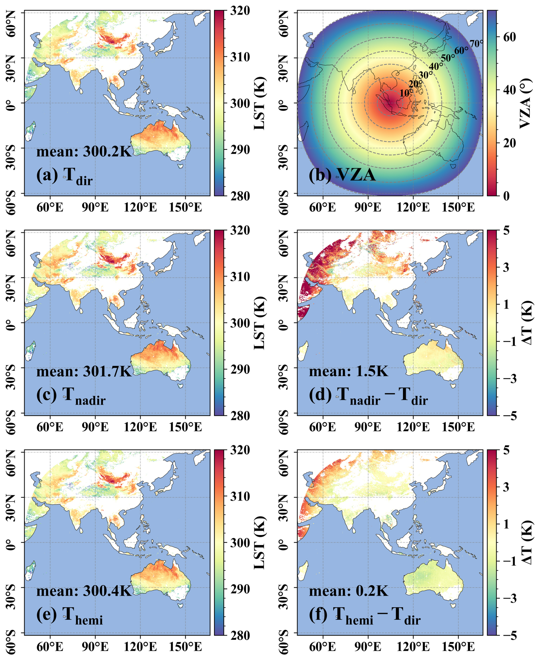
Figure 4 The spatial distribution of (a) directional LST, (b) VZA, (c) nadir LST, (d) LST difference between nadir and directional LST, (e) hemispherical LST, and (f) LST difference between hemispherical and directional LST on 24 June 2020 at 03:00 UTC.

4 Results

4.1 Results of angular normalization

Figure 4 shows the spatial distributions of FY-4A directional LST (T_dir), FY-4A VZA, normalized nadir LST (T_nadir), the LST difference between T_nadir and T_dir, hemispherical LST (T_hemi), and the difference between T_hemi and T_dir on 24 June 2020 at 03:00 UTC (i.e., the Beijing time of 11:00 BJT). As shown in Fig. 4c, T_nadir is 1.5 K larger than T_dir on average. It closely resembles T_dir (with a small value of T_nadir−T_dir) when the VZA is within 40°, and becomes significantly higher than T_dir as VZA increases, with a correction value of T_nadir−T_dir exceeding 5 K near the edge of the FY-4A disk as shown in Fig. 4d. When the VZA is small, the observation angle of FY-4A is close to the nadir direction, resulting in a small correction value from T_dir to T_nadir. However, more cool vegetated elements were viewed at large VZA (i.e., the well-known gap fraction effect), which resulted in a much lower T_dir than T_nadir and further led to a larger angular correction value. For hemispherical LST, the T_hemi (Fig. 4e) is only 0.2 K higher than T_dir on average. It is approximately 2 K lower than T_dir (Fig. 4a) in Australia, while being very close to T_dir in northern China. At the edge of the FY-4A disk, T_hemi is around 3 K higher than T_dir (where the VZA exceeds 60°, see Fig. 4b and f). This spatial pattern can be partially explained by the value of the hemispherical equivalent angle (i.e., the VZA at which T_dir=T_hemi), which has been reported to range from 44 to 53° in relevant studies (Hu et al., 2023; Zhang et al., 2025). When the VZA is smaller than 44°, T_dir tends to be higher than T_hemi because more hot soil components are viewed. Conversely, for large VZAs over 53° (e.g., at the edge of FY-4A disk), T_dir becomes lower than T_hemi as more cool vegetation components are viewed.

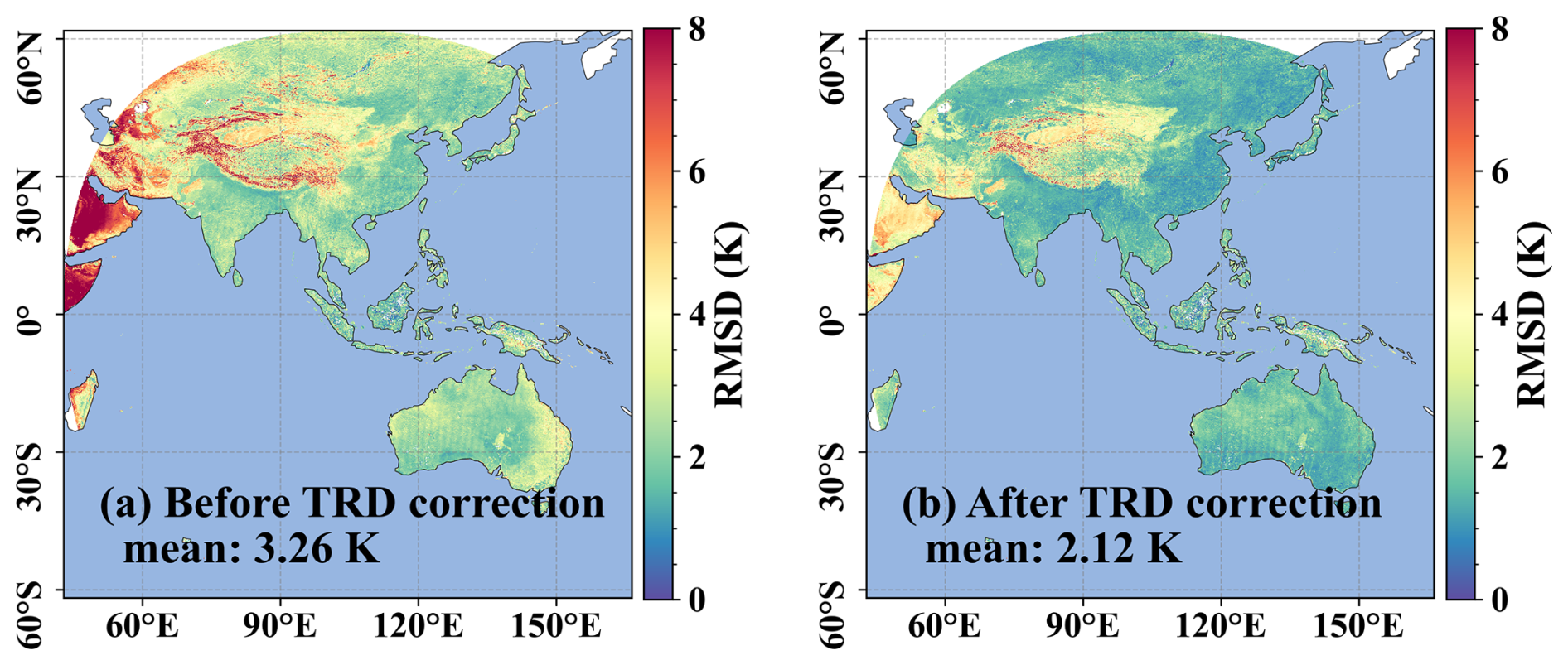
Figure 5 Spatial distribution of RMSD between FY-4A and MODIS (a) before and (b) after TRD correction.

There will be significant inconsistencies in directional LST between FY-4A and MODIS due to the TRD effect. Figure 5a quantifies this discrepancy by presenting the RMSD between FY-4A and MOD11A1 directional LST. After correcting both LST products to nadir values, the corresponding RMSD is shown in Fig. 5b. The average RMSD across the full FY-4A disk decreases from 3.26 to 2.12 K, representing a reduction of 1.14 K (35.0 %). The extremely high values near the western edge of the disk are substantially reduced after correction. However, relatively high values over the western Qinghai–Tibetan Plateau persist, which may be partly attributed to limitations of the employed LSF-Chen model, as it is derived under the assumption of flat terrain. Overall, the TEKDM demonstrates strong performance in reducing angular inconsistencies between LST products as expected.

The cross-validation between FY-4A T_dir, T_nadir, and the VNP21A1 near-nadir LST (i.e., the VZA < 5°) in 2020 is shown in Fig. 6. The root mean squared difference (RMSD) and mean bias difference (MBD) are 4.53 and −1.85 K for T_dir as shown in Fig. 6a. After angular normalization, the RMSD and MBD for T_nadir is 2.56 and 0.06 K as shown in Fig. 6b, with a 1.97 K (i.e., 43.5 %) reduction in RMSD and an almost unbiased MBD. Figure 6c shows the RMSD values of T_dir and T_nadir across different VZA intervals with a step of 10°. The RMSD difference between them remains within 0.2 K when VZA is less than 40°. However, when VZA exceeds 40°, the RMSD for T_dir increases substantially (from 3.4 to 6.5 K), while the RMSD for normalized T_nadir remains lower than 3.0 K for large VZA. The higher RMSD of T_dir at large VZA can be partially attributed to its significant underestimation as shown in Fig. 6d. The MBD of T_dir exceeds −3.8 K when the VZA is between 60 and 70°, whereas that of the normalized T_nadir is 0.9 K. The gap fraction effect could explain this angular dependence of MBD, i.e., a larger VZA leads to a smaller T_dir compared with nadir LST.

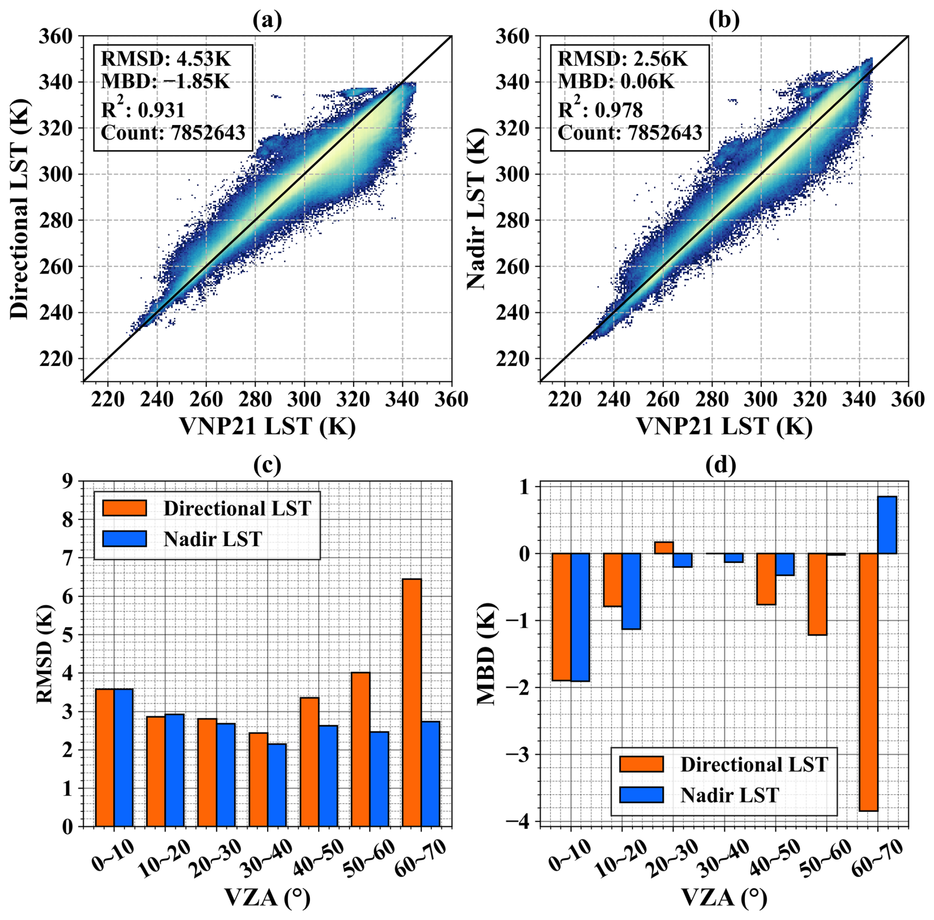
Figure 6 The cross-validation of (a) directional and (b) nadir LST against VNP21 near-nadir LST at 0.05° resolution. The angular variation of (c) RMSD and (d) MBD for directional and nadir LST at 0.05° resolution.

The evaluation of 0.05° FY-4A T_dir and T_hemi during daytime over 8 stations is shown in Fig. 7a and b. Results show that the RMSE decreased from 2.22 to 2.00 K, with an improvement of 0.22 K. The MBE changed from 0.19 to −0.54 K. For the temperatures between 280 to 300 K with the highest density, the scatter points become closer to the 1:1 line after the angular normalization. Figure 7c and d shows the RMSE and MBE of FY-4A T_dir and T_hemi at different local times. T_dir exhibits a pronounced overestimation with higher RMSE in the morning, and an underestimation with smaller RMSE in the afternoon. After the angular normalization, the T_hemi shows significantly improved performance in the morning, with an RMSE reduced by approximately 0.4–0.8 K (Fig. 7c). As shown in Fig. 7d, the MBEs of T_hemi are much smaller than those of T_dir in the morning, with a maximum reduction of 1.7 K at 11:00 LT.

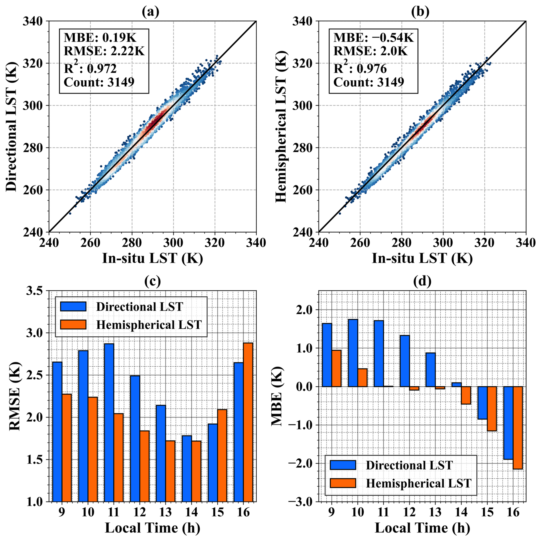
Figure 7 The accuracy of FY-4A (a) directional LST, (b) hemispherical LST, and the temporal variation of (c) RMSE and (d) MBE for directional and hemispherical LST.

4.2 Results of all-weather LST estimation

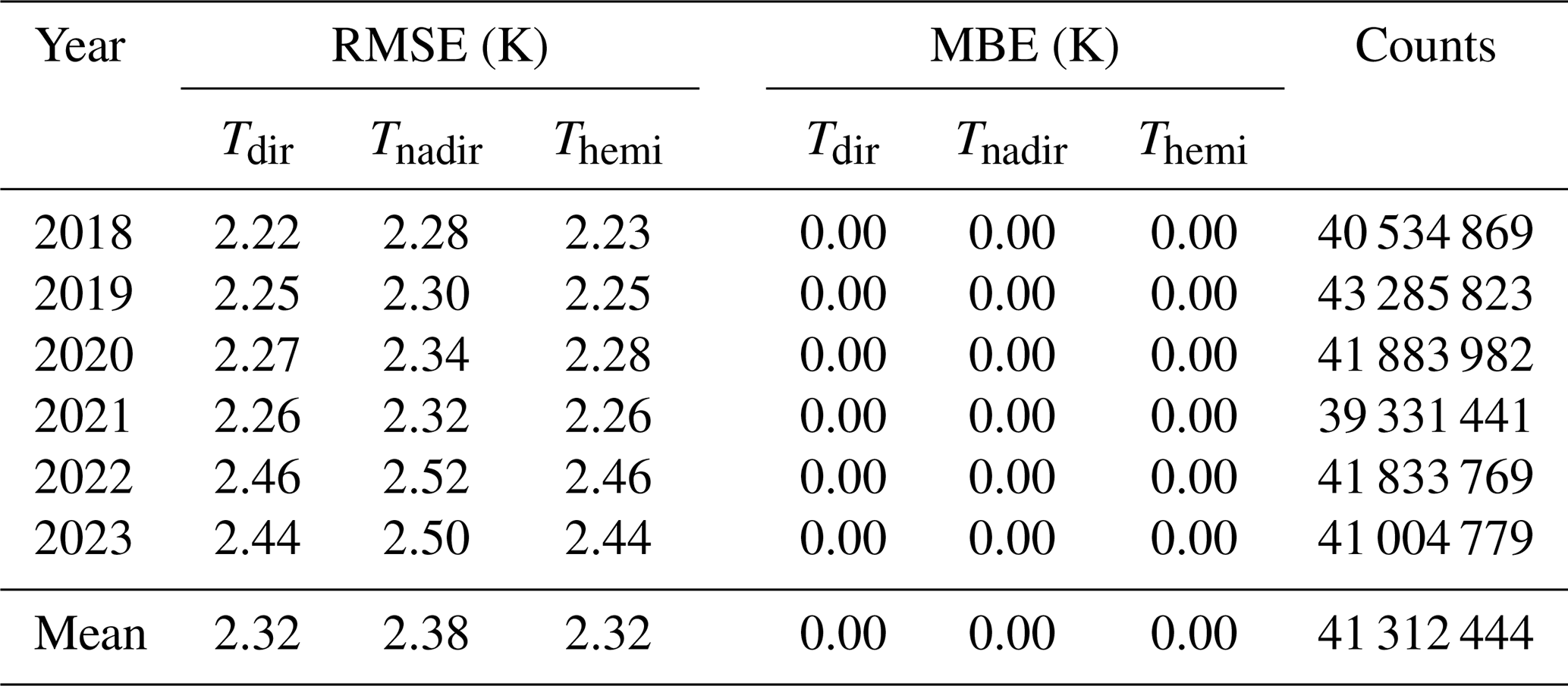
The prediction accuracy of f_clr in reconstructing hypothetical clear-sky T_dir, T_nadir, and T_hemi over the test set from 2018 to 2023 is summarized in Table 3. The average annual number of samples is 41 312 444. The RMSE ranges from 2.22 to 2.46 K for T_dir, from 2.28 to 2.52 K for T_nadir, and from 2.23 to 2.46 K for T_hemi. RMSE values remain relatively stable from 2018 to 2021, followed by an increase of approximately 0.2 K during 2022–2023. On average, the RMSE for T_dir is 0.06 K lower than that for T_nadir, and is the same as that for T_hemi, indicating comparable fitting performance across different CatBoost models. The MBE is zero for all models, indicating that no significant systematic bias was introduced in the predicted hypothetical clear-sky LST.

Table 3 The prediction accuracy for reconstructing hypothetical clear-sky directional, nadir, and hemispherical LST.

Spatial heterogeneity in LST can lead to variations in model performance. The pixel-level RMSE of the CatBoost model for 2020 was evaluated by comparing the CatBoost-predicted hypothetical nadir LST with the normalized FY-4A nadir LST. The nadir configuration is well suited for quantifying the performance of ML model, because it minimizes systematic uncertainties associated with angular effects. As shown in Fig. 8, the mean RMSE of the cloud-filling results is 2.49 K. Higher uncertainties are observed over regions such as the Qinghai–Tibet Plateau and the Indonesian Peninsula, which can likely be attributed to persistent cloud cover. In such regions, the reduced availability of clear-sky observations limits the training samples, leading to increased uncertainty in the machine learning model performance.

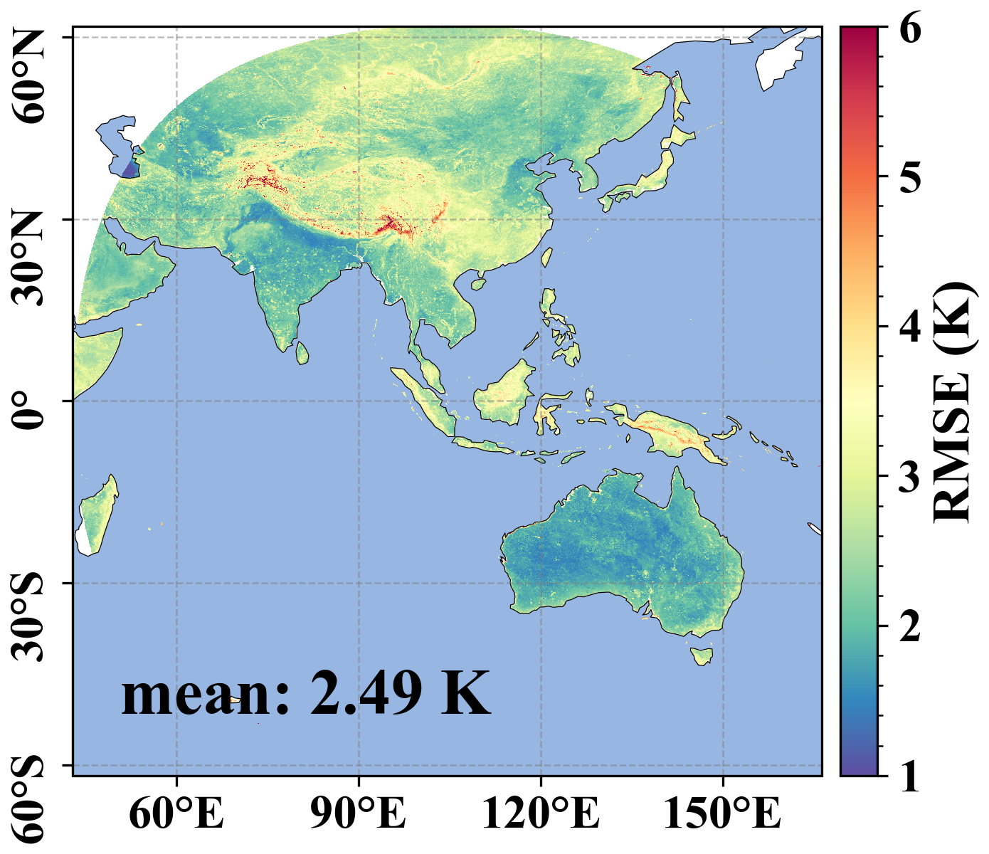
Figure 8 Pixel-level prediction RMSE of the CatBoost model in 2020.

The estimated 0.05° all-weather T_hemi results were further evaluated by the in situ hemispherical LSTs from 8 in situ stations (Fig. 9). The samples are divided into clear-sky (Fig. 9a) and cloudy-sky (Fig. 9b) conditions. The “3σ-Hampel identifier” method was applied to minimize the influence of outliers at each site. Both daytime and nighttime T_hemi values were considered here. Under clear-sky conditions, 0.05° T_hemi shows an RMSE of 2.48 K and an MBE of −0.83 K. The distribution of residuals ($\mathrm{\Delta }\mathrm{LST}=T_{\mathrm{hemi}}-T_{\mathrm{insitu}}$) approximately follows a normal distribution. Under cloudy-sky conditions, T_hemi shows a higher RMSE of 3.65 K and a more significant negative MBE of −1.43 K. It is challenging to maintain the same level of accuracy under cloudy-sky conditions, as uncertainties in both the CatBoost-predicted hypothetical LST and the estimated ΔT_CRF are introduced.

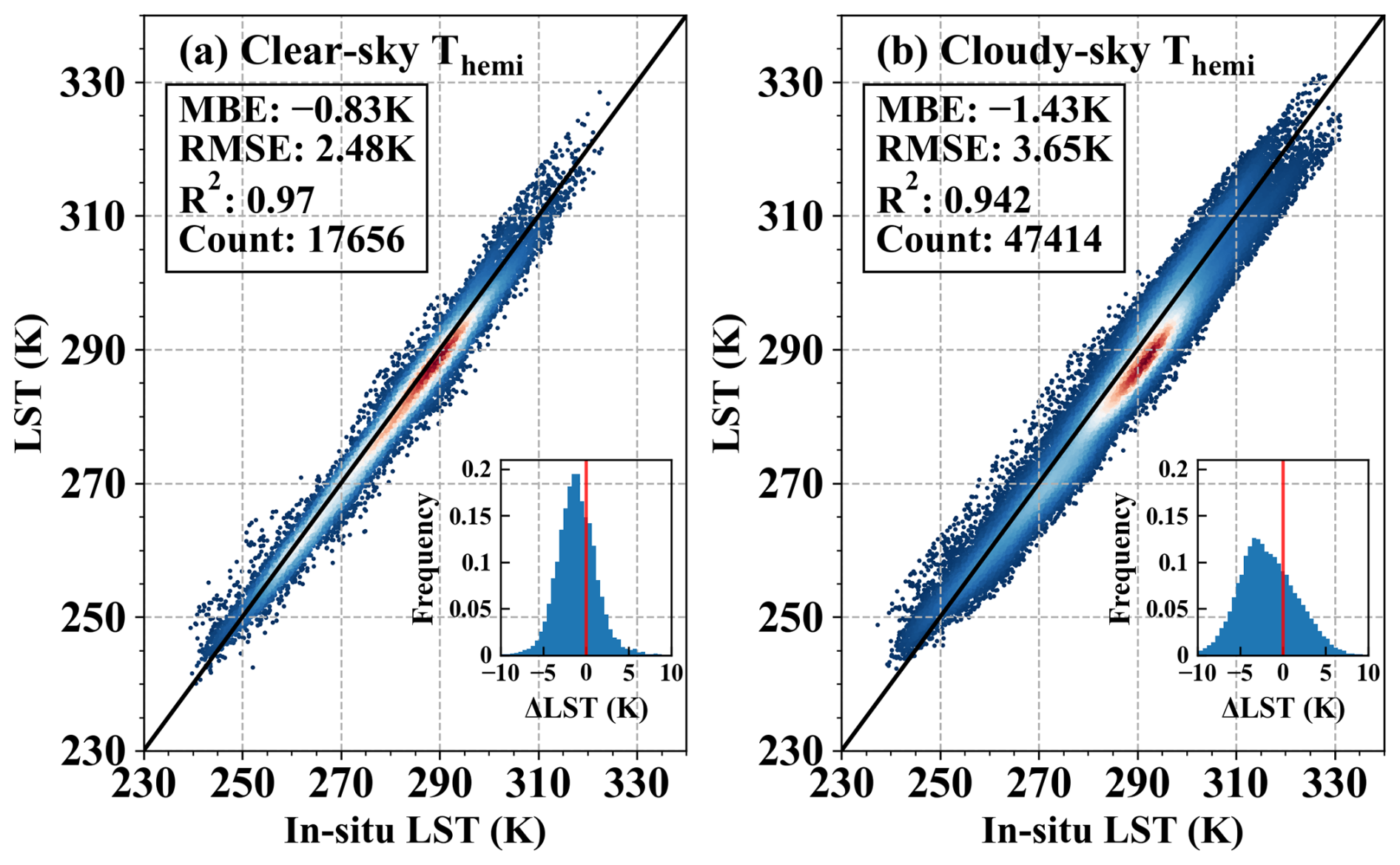
Figure 9 The accuracy of all-weather hemispherical LST under (a) clear-sky and (b) cloudy-sky condition.

Figure 10a and b shows the temporal consistency of FY-4A official LST, T_hemi, and in situ LST at the DM and SDQ sites throughout 2020 at 04:00 and 16:00 UTC (i.e., 12:00 and 00:00 BJT). Overall, the all-weather T_hemi agrees well with the in situ LST. At the DM site during daytime (Fig. 10a), the clear-sky RMSE (MBE) of FY-4A official LST is 3.20 K (2.43 K), whereas the corresponding values for T_hemi are 2.15 K (0.46 K), indicating that the systematic overestimation is significantly mitigated after angular normalization. Similarly, at the SDQ site during daytime (Fig. 10b), the clear-sky RMSE (MBE) decreases from 4.77 K (4.02 K) for the FY-4A official LST to 3.60 K (2.55 K) for T_hemi. During nighttime, the clear-sky T_hemi is the same as FY-4A official LST, showing lower RMSE values than during daytime. The RMSE (MBE) values are 2.38 K (−0.94 K) at the DM site and 2.2 K (−0.17 K) at the SDQ site. Under cloudy-sky conditions, the RMSE (MBE) values are 3.54 K (−0.53 K) at the DM site and 4.09 K (1.97 K) at the SDQ site during daytime, and 4.58 K (−3.77 K) at the DM site and 3.46 K (−1.36 K) at the SDQ site during nighttime. In summary, the all-weather LST could effectively capture the characteristics of the annual temperature cycle.

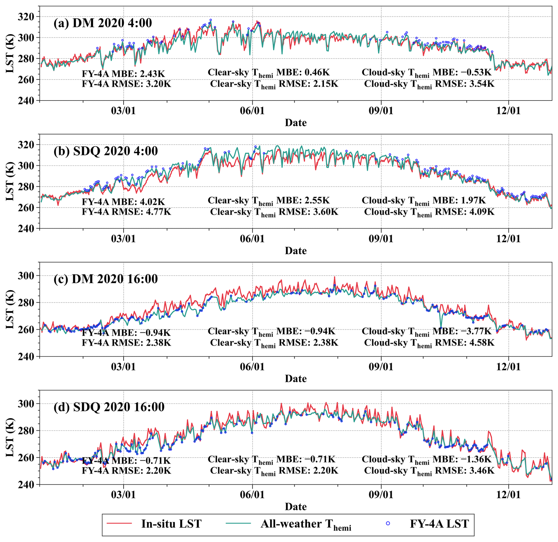
Figure 10 The temporal variation trend of in situ LST, T_hemi, and FY-4A official LST in 2020 for (a) DM site at 04:00 UTC, (b) SDQ site at 04:00 UTC, (c) DM site at 16:00 UTC, (d) SDQ site at 16:00 UTC. Note that the clear-sky T_hemi is the same as FY-4A LST during nighttime because the TRD effect is ignored at night.

4.3 Results of spatial downscaling

In the spatial resolution downscaling process, the CatBoost model was used to establish the relationship between regression kernels and the LST difference (e.g., the satellite LST minus ATC-simulated LST) at 0.05° resolution. The prediction accuracy of each month over the test set from 1 January 2018 to 31 December 2023 for daytime and nighttime conditions is shown in Fig. 11. The nighttime RMSE ranges from 1.8 to 2.4 K, which is consistently lower than the daytime RMSE (2.6–3.1 K). This discrepancy can be partially attributed to the fact that daytime LST tends to be more heterogeneous than nighttime LST, leading to greater modeling errors during the day. The daytime RMSE increases from January to May and then decreases. In contrast, the nighttime RMSE decreases from January to July and then rises. The RMSE difference among directional, nadir, and hemispherical LST are within 0.2 K. Overall, the results demonstrate the reliable capability of the CatBoost model in the spatial resolution downscaling.

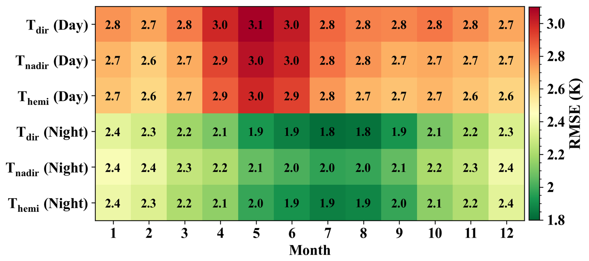
Figure 11 The prediction RMSE over test set for directional, nadir, and hemispherical LST during both daytime and nighttime for each month.

The spatial distribution of prediction accuracy for the machine learning model during the downscaling process is presented in Fig. 12, where the RMSE was calculated between the CatBoost-estimated LST and the input all-weather nadir LST. The overall RMSE is 2.28 K, with higher values predominantly observed in mountainous regions, likely due to enhanced surface heterogeneity and elevation-induced variability. It should be noted that clear-sky pixels remain unchanged in the all-weather LST product; therefore, the ANCFDS-LST for these pixels is affected only by uncertainties introduced during the downscaling step. In contrast, for cloud-contaminated pixels, the final LST incorporates uncertainties arising from both the cloud-filling and downscaling processes.

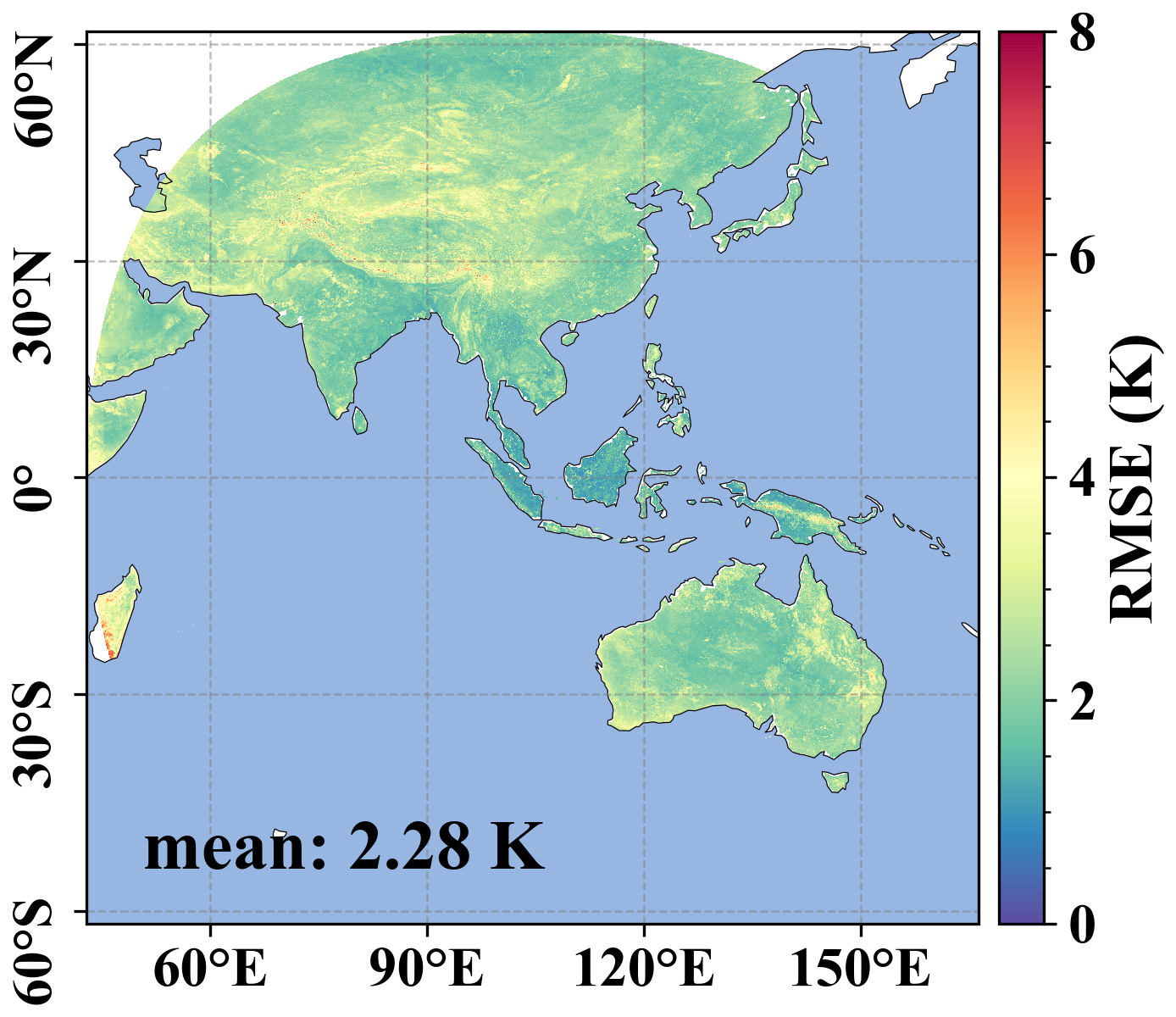
Figure 12 Spatial distribution of prediction RMSE for nadir LST over the test set in 2020.

Downscaled LST is expected to exhibit enhanced spatial texture, which is quantitatively evaluated in this study. The local variance ratio (LVR) and the structural similarity index (SSIM) were employed as metrics to compare the spatial textures of bilinearly interpolated LST (derived from 0.05° all-weather LST) and the downscaled 0.01° nadir LST. Values of LVR and SSIM closer to 1 indicate a higher similarity between the reconstructed and reference spatial textures. The reference texture was reconstructed using the ATC model, which also provided the prior thermal texture information during downscaling. Therefore, the LVR and SSIM metrics mainly evaluate the consistency and preservation of the prescribed ATC-based spatial texture (Jia et al., 2024), rather than serving as an independent assessment of sub-pixel LST accuracy. As shown in Fig. 13, the median LVR increases from 0.41 to 0.97, while the median SSIM improves from 0.83 to 0.91, indicating that the downscaled LST better preserves the imposed spatial texture characteristics than bilinear interpolation.

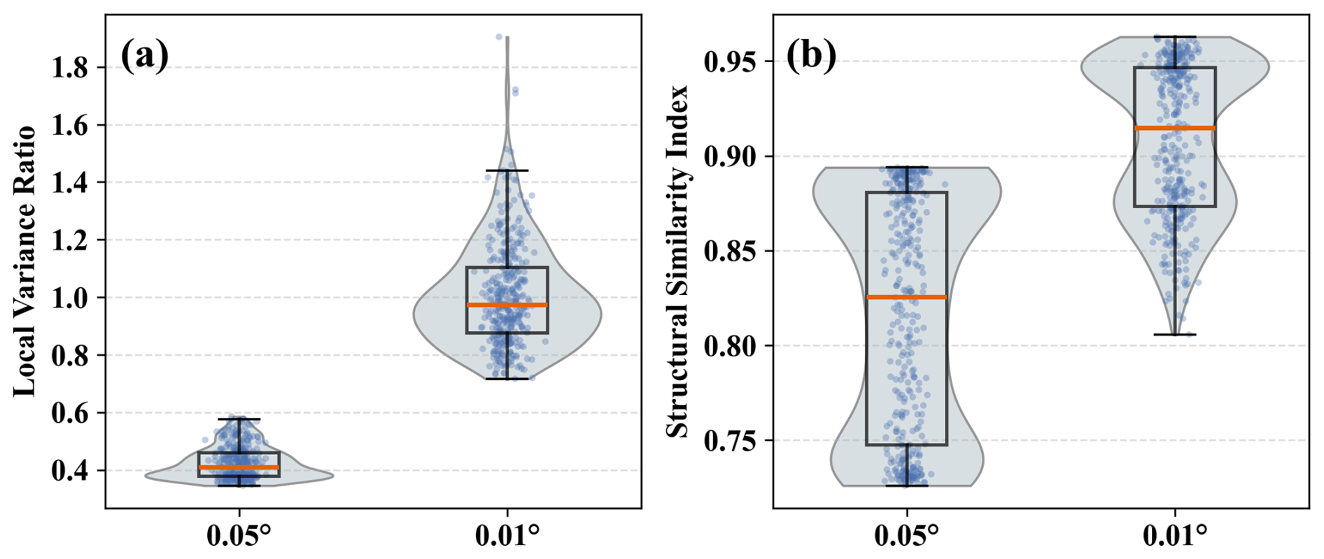
Figure 13 (a) Local variance ratio and (b) structural similarity index between bilinearly interpolated LST and the downscaled 0.01° nadir LST, with ATC-simulated LST used as the reference.

T-based validation results for the all-weather T_hemi product before and after downscaling are presented in Fig. 14. The RMSE remained unchanged at 3.34 K for both the 0.05 and 0.01° resolutions, while the MBE changed only marginally from −1.27 to −1.28 K. These nearly identical validation statistics suggest that the downscaling procedure introduces minimal additional uncertainty. This consistency can be attributed to two main factors. First, the downscaling framework employs a residual redistribution strategy, which preserves the large-scale thermal information of the original 0.05° LST product. As a result, the accuracy of the downscaled 0.01° T_hemi product remains strongly constrained by the performance of the original coarse-resolution LST. Second, the validation sites were rigorously screened to ensure strong spatial representativeness at both the 0.05 and 0.01° scales. Consequently, the retrieved LSTs at the two spatial resolutions are expected to exhibit comparable validation accuracy.

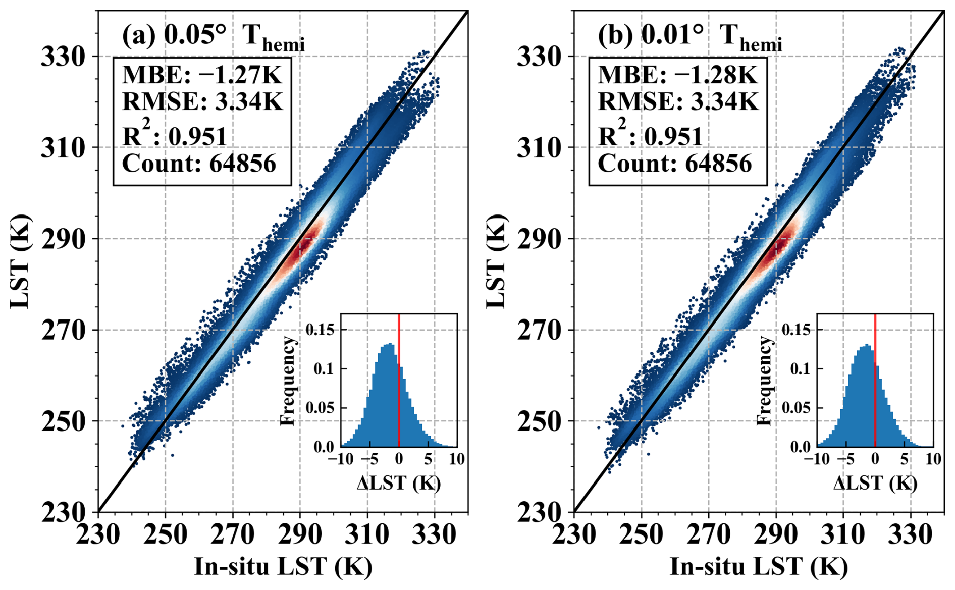
Figure 14 The accuracy of all-weather hemispherical LST products (a) before and (b) after downscaling.

The spatial distributions of all-weather T_nadir and T_hemi at 0.05 and 0.01° resolutions on 24 June 2020 at 04:00 UTC (12:00 BJT) are presented in Fig. 15. Two representative regions are highlighted for detailed comparison: the western Tibetan Plateau (red rectangles in Fig. 15a–d) and the Greater Khingan Mountains (blue rectangles in Fig. 15a–d). As shown in Fig. 15a–d, the large-scale spatial patterns of LST are well preserved after downscaling, with both T_nadir and T_hemi exhibiting clear latitudinal and elevational gradients (i.e., lower temperatures are consistently observed in high-latitude and high-altitude regions). T_hemi integrates directional LST values over all viewing angles and thus generally shows smoother spatial variability than T_nadir. At finer scales (Fig. 15e–l), the downscaled results (0.01°) reveal substantially enhanced spatial details compared to the coarse-resolution counterparts. In particular, complex terrain features become more distinguishable, such as ridge–valley structures over the Tibetan Plateau and the heterogeneous forest–grassland patterns in the Greater Khingan Mountains. The contrast between sunlit and shaded slopes, as well as between higher and lower elevations, is more pronounced in the downscaled LST fields. These improvements in spatial texture and terrain-related variability demonstrate the effectiveness of the IHDA downscaling method in capturing fine-scale thermal heterogeneity.

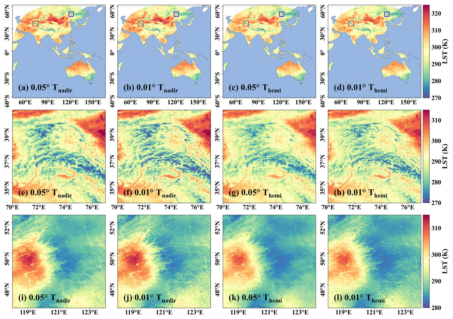
Figure 15 Spatial distributions of nadir LST at 0.05° (a, e, i) and 0.01° (b, f, j), and hemispherical LST at 0.05° (c, g, k) and 0.01° (d, h, l) at 04:00 UTC on 24 June 2020. The first row (a–c) shows LST over the FY-4A full disk, the second row (e–h) over the western Qinghai–Tibetan Plateau, and the third row (i–l) over the Greater Khingan Mountains.

5 Discussion

5.1 The temporal aggregation method for KDM parameters

In this study, a temporal aggregation method spanning 8 d before and after the target day (a total of 17 d) was employed to aggregate the KDM parameters (i.e., α, β, and W). It not only filtered out extreme values in the TEKDM results but also filled the gaps for pixels where TEKDM could not be solved. The 17 d compositing method was comprehensively compared with three other aggregation approaches: (1) 9 d composition: averaging values from four days before and after the target day (a total of 9 d). (2) Monthly composition (i.e., ∼30 d in total): calculating the monthly average of KDM parameters, assuming they remain constant throughout each month. (3) Yearly composition (i.e., ∼365 d in total): calculating the yearly average of KDM parameters, assuming they remain constant throughout the whole year. After calibrating the KDM parameters using each approach, FY-4A directional LST could be normalized to T_nadir. Then, the 2020 T_nadir results were cross-validated using VNP21A1 near-nadir LST (i.e., VZA < 5°), following the same procedure as in Fig. 6.

Figure 16a–e shows the cross-validation results between the $T_{\mathrm{dir}}/T_{\mathrm{nadir}}$ and VNP21A1 near-nadir LST, whereas Fig. 16f shows the valid pixel fraction (i.e., the ratio of pixels with valid KDM parameters to the total number of clear-sky land surface pixels) for the above temporal aggregation methods. The RMSD (MBD) of the FY-4A official LST is 4.53 K (−1.85 K), while the RMSD (MBD) for the four compositing methods ranges from 2.53 to 2.66 K (−0.12 to 0.07 K). The RMSD values in ascending order are: monthly method < 17 d method < 9 d method < yearly method. In terms of valid pixel fractions, the order is the 9 d method (89.3 %) < 17 d method (93.6 %) < monthly method (95.9 %) < yearly method (99.5 %). The significant lower valid pixel fractions for the 9 and 17 d methods in August 2020 (Fig. 16f) are attributed to the absence of MYD11A1 LST products between 16 and 31 August 2020 (induced by a Formatter-Multiplexer Unit/Solid State Recorder (FMU/SSR) error, more details can be found at https://atmosphere-imager.gsfc.nasa.gov/issues/l1b#Issue01, last access: 16 June 2026). The yearly method was not adopted since it has the largest RMSD, whereas the 9 d method was not used since it has the lowest valid pixel fraction. The 17 d and monthly methods could achieve comparable and acceptable accuracy. The 17 d method was ultimately selected with reference to parameter aggregation approaches commonly used in the optical remote sensing domain (Liu et al., 2013).

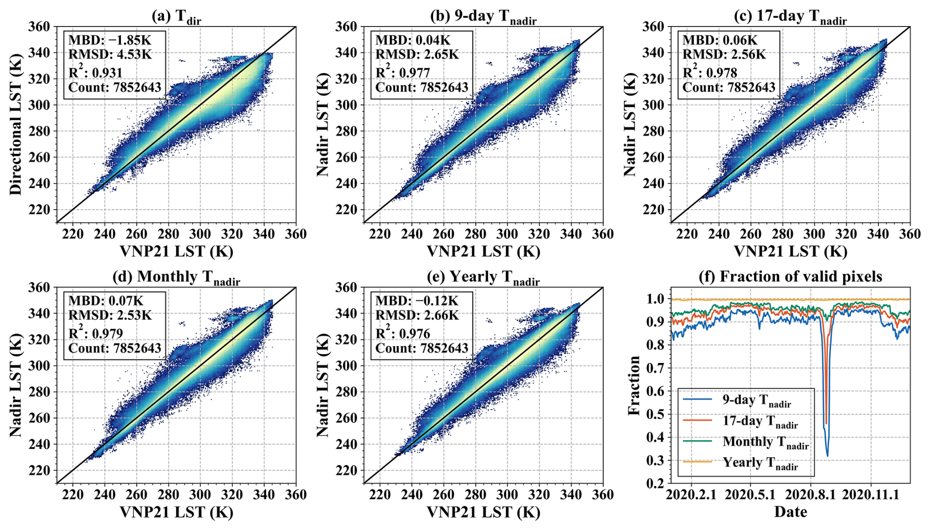
Figure 16 The cross-validation results of (a) FY-4A directional LST, (b) T_nadir generated using 9 d composition method, (c) using 17 d composition method, (d) using monthly composition method, (e) using yearly composition method. (f) The fraction of valid pixels for different composition methods.

5.2 Feature Importance for CatBoost models in hypothetical clear-sky LST estimation and LST downscaling

The relative feature importance of the CatBoost model was determined based on each feature's contribution to the reduction of the loss function. We employed the logarithmic value of (1 + score_norm) to quantify the importance of each model (where score_norm is the max-min normalized feature scores). The average relative feature importance across all CatBoost models is shown in Fig. 17. In the estimation of hypothetical clear-sky LST (Fig. 17a), T_ERA5-skin exhibited the highest importance. The T_2 m and R_in were also identified as influential predictors, aligning with the findings of Zhang et al. (2024). The θ_s accounted for a significant 9.9 % of the importance, reflecting the strong influence of solar radiation on LST. Most other features had relatively low importance (below 5 %), and ATC${}_{{\mathrm{d}}_{\mathrm{1}}}$, CT, FVC, and LCT contributed less than 1 %. In the LST downscaling task from 0.05 to 0.01° using CatBoost model (Fig. 17b), the ATC-simulated LST at the initial time had the highest importance of 30.8 %. The air temperature (T_2 m) and MAST${}_{{\mathrm{d}}_{\mathrm{2}}}$ also had high importance exceeding 10 %. The YAST${}_{{\mathrm{d}}_{\mathrm{2}}}$, DEM, and $\mathrm{d}{x}_{{\mathrm{n}}_{\mathrm{2}}}$ showed moderate importance between 5 % and 10 %, while the $\mathrm{d}{x}_{{\mathrm{d}}_{\mathrm{2}}}$, MAST${}_{{\mathrm{n}}_{\mathrm{2}}}$, and YAST${}_{{\mathrm{n}}_{\mathrm{2}}}$ contributed less than 5 %. Eliminating those features with low importance has the potential to enhance computational efficiency and reduce dependency on related auxiliary datasets, which should be carefully assessed in future studies.

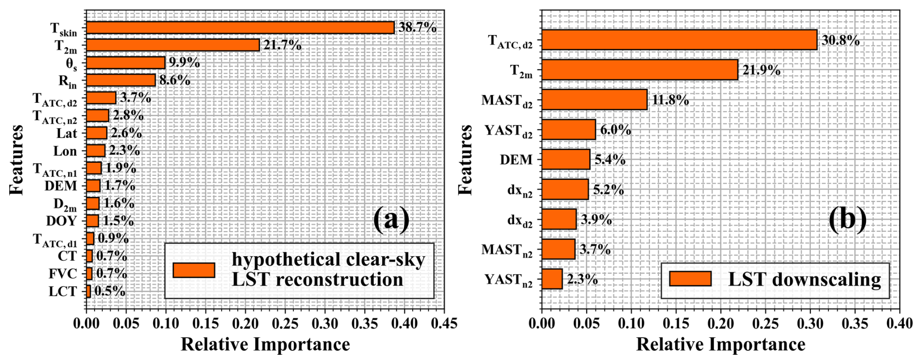
Figure 17 The relative importance for the CatBoost model when (a) estimating the hypothetical clear-sky LST using Eq. (13), and (b) downscaling the 0.05° LST difference using Eq. (18).

5.3 The spatial representativeness of in situ sites

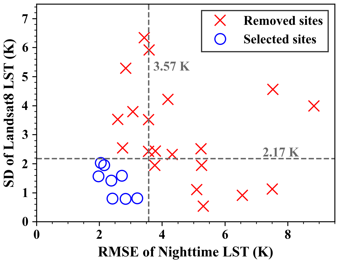
T_nadir was evaluated against near-nadir LST from VNP21A1, whereas the 0.05° T_hemi product was validated using in situ measurements. The T-based validation of T_hemi requires in situ sites with high spatial representativeness. To this end, the spatial heterogeneity of 11 HiWATER sites, 11 OzFlux sites, and 6 sites over the Tibetan Plateau in 2020 was assessed (Beringer et al., 2016; Che et al., 2019; Ma et al., 2024b). Following Zhang et al. (2024), two metrics were adopted: (1) the median standard deviation (SD) of Landsat 8 LST within a 0.05° window, and (2) the RMSE between nighttime FY-4A LST and in situ LST. Sites that substantially deviated from the median values of these two indicators were excluded, as illustrated in Fig. 18. Ultimately, 8 out of 28 candidate sites were retained, all satisfying the criteria of nighttime RMSE < 3.57 K and SD < 2.17 K.

Figure 18 The spatial representativeness evaluation of the employed in situ sites.

5.4 The inter-comparison with other all-weather LST products

The inter-comparison between the generated all-weather T_hemi product and four existing all-weather LST products against in situ LST measurements in 2020 is shown in Fig. 19. Although the absolute accuracy is influenced by the spatial representativeness of in situ sites as analyzed in Sect. 5.3, the relative accuracy of different LST products is comparable. Two of the employed datasets are reanalysis products: ERA5-Land LST at 0.1° resolution and China Land Surface Data Assimilation System (CLDAS) LST at 0.0625° resolution. Additionally, two remote sensing products were included: a global all-weather 0.05° LST dataset generated by Jia et al. (2023), and a regional 0.02° LST product for East Asia region developed by Dong et al. (2022). Jia's method first estimates hypothetical clear-sky LST using a Kalman filter with ERA5, Himawari-8 and MODIS LSTs as inputs. An iterative CRF correction is then applied to produce the cloudy-sky LST. Dong's approach first retrieves clear-sky LST from Himawari-8 using a TES algorithm, and then estimates cloudy-sky LST using a multiresolution Kalman filter based on CLDAS LST. For consistency, all four products were resampled to 0.05° resolution to match the 0.05° T_hemi for inter-comparison, and only HiWATER sites were used due to the limited spatial extent of CLDAS LST. Under clear-sky conditions (Fig. 19a), ERA5 and CLDAS show similar accuracy with RMSE values of 4.2–4.5 K during the day and 4.2 K at night. Our T_hemi product has superior accuracy with RMSE values of 2.3 K during both day and night. Dong's LST shows accuracy comparable to T_hemi, whereas Jia's LST exhibits RMSE values between those of the reanalysis products and T_hemi. Under cloudy-sky conditions (Fig. 19b), ERA5 LST has the lowest accuracy with an RMSE of 5.2 K during the day and an RMSE of 4.1 K at night. CLDAS LST has RMSEs of 5.1 K during daytime and 4.0 K at night, which performs worse than remote sensing-based LST. The RMSE of T_hemi is comparable to that of Jia's LST, but lower than that of Dong's LST. The overall performance of the T_hemi product under both clear-sky and cloudy-sky conditions demonstrates its strong potential for subsequent applications.

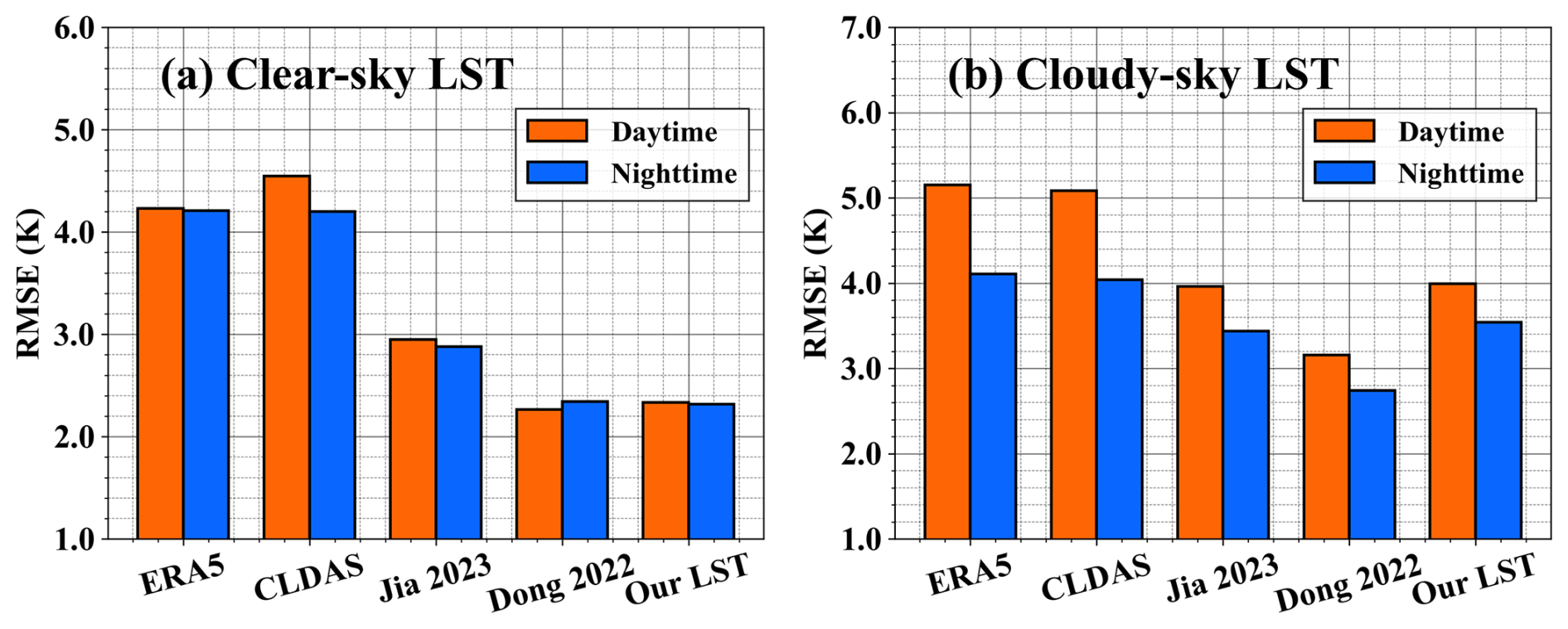
Figure 19 The RMSE comparison of five products during the day and night under (a) clear-sky condition and (b) cloudy-sky condition.

5.5 Limitations and future work

The evaluation results of the generated ANCFDS-LST demonstrate its high accuracy and detailed texture. Several limitations remain to be addressed in future work:

1. The TEKDM used in this study is developed for vegetated canopies, which is dominated by the gap fraction and hot spot effects. However, the applicability of this model to other land covers, such as bare soil, snow, and urban areas, requires further exploration and validation (Du et al., 2023, 2024; Wang et al., 2024a; Xiong et al., 2024). Moreover, the reliability of TEKDM in complex terrain also demands in-depth studies (Zhan et al., 2025).

2. The nighttime TRD effect was neglected in this study, as LST is generally more homogeneous within a pixel and angular effects are typically weak under nighttime conditions (Na et al., 2024a). However, TRD effects may persist in geostationary observations shortly after sunset (Jiang et al., 2022). Modeling daytime and nighttime TRD effects separately is a promising approach for improving nighttime angular normalization; however, this strategy has not yet been implemented in the current TEKDM framework. Therefore, the development of an advanced TEKDM that explicitly accounts for nighttime TRD effects warrants further investigation in future studies.

3. Thermal infrared directional anisotropy is primarily governed by canopy structure and surface thermal heterogeneity, the latter being strongly affected by solar illumination and the resulting temperature contrast between soil and vegetation components. Under cloudy conditions, direct solar radiation is reduced, while diffuse radiation and atmospheric longwave emission increase, which tends to weaken the magnitude of TIR directional anisotropy. However, the weakened TRD effect is strongly influenced by cloud optical properties, cloud duration, and atmospheric humidity, making it difficult to model using physical approaches. Future studies should incorporate multi-angle observations under cloudy-sky conditions to better characterize TRD effects under cloud cover (Jia et al., 2024).

4. In this study, a sinusoidal ATC model was employed to provide auxiliary thermal texture information. However, this approach may introduce uncertainties in tropical regions, where LST typically exhibits bimodal seasonal cycles with two annual peaks. Previous studies have attempted to address this limitation by incorporating dual-sinusoidal functions (Xing et al., 2020). In future work, the adoption of more accurate and universally applicable ATC models would be beneficial for improving the robustness of cloudy-sky LST estimation and downscaling.

5. This study extensively employs machine learning methods driven by reanalysis products. Although the primary observational constraints are derived from remote sensing products, uncertainties in the inputs may still propagate through the cloudy-sky LST estimation and downscaling processes. In future studies, developing robust error quantification techniques would aid in tracing how uncertainties in input parameters influence the final 0.01° all-weather LST, thereby further refining the ANCFDS-LST product (Li et al., 2024b).

6. The T-based validation in this study is based on 8 in situ sites from HiWATER and OzFlux networks, which inevitably introduces uncertainty due to their limited representativeness across land cover types. Future studies could incorporate radiance-based (R-based) validation to mitigate this issue, offering a valuable complement to T-based validation (Li et al., 2021).

6 Data availability

The hourly 0.01° all-weather T_dir, T_nadir, and T_hemi product (ANCFDS-LST) from 2018 to 2023 is freely available at https://doi.org/10.11888/RemoteSen.tpdc.303249 (Na et al., 2026). Data are stored in GeoTIFF format with three sequential bands (T_dir, T_nadir, and T_hemi, respectively), and the units of each file is kelvin. A scale factor of 0.1 and offset of 0 have been applied for value encoding. Quality check (QC) flags are also provided. A value of 1 indicates clear-sky LST with angular normalization applied, whereas a value of 0 denotes reconstructed LST generated using the all-weather estimation procedure.

7 Conclusion

In this study, an angular-normalized, cloud-filled, and 0.01° downscaled LST was generated from 2018 to 2023 based on the official FY-4A LST dataset. Firstly, a TEKDM-based angular normalization method was used to generate nadir and hemispherical LST products. Secondly, an all-weather LST estimation approach was adopted to produce 0.05° cloud-filled directional, nadir, and hemispherical LST. Finally, an IHDA method was employed to enhance the spatial resolution of the LST products from 0.05 to 0.01°. The main conclusions are summarized as follows:

1. The TEKDM model significantly normalized the angular dependence of daytime clear-sky T_dir. Taking the near-nadir VNP21A1 LST as reference, the RMSD (MBD) decreased from 4.53 K (−1.85 K) of the T_dir to 2.56 K (0.06 K) of normalized 0.05° T_nadir. Taking the in situ hemispherical LSTs in the Heihe River Basin and Australia as reference, the RMSE decreased from 2.22 K of the T_dir to 2.00 K of the normalized 0.05° T_hemi.

2. For the all-weather 0.05° T_hemi, the T-based validation shows an RMSE of 2.48 K under clear-sky conditions and 3.65 K under cloudy-sky conditions. The generated all-weather T_hemi shows comparable accuracy with the existing four all-weather LST products (i.e., ERA5, CLDAS, Jia2023 and Dong2022). After downscaling, the 0.01° all-weather LST successfully recovered fine spatial details.

Although the generated directional, nadir, and hemispherical LST products exhibit high accuracy and rich spatial texture, their spatial coverage is currently limited to the FY-4A disk. Further work is needed to expand this methodology for producing global-scale LST products, e.g., gathering Himawari, GOES and MSG satellite datasets. In addition, the T-based validation was performed over limited in situ sites in this study, and a more comprehensive approach such as R-based validation is still lacking. Future research should focus on performing robust validation over more land covers and also over complex terrains.

Appendix A

Accurate numerical integration for deriving T_hemi is computationally expensive. To improve efficiency, a polynomial fitting approach was adopted to approximate the exact integration. As shown in the numerator of Eq. (12), the integration involved in estimating T_hemi depends only on α, β, W, and SZA. Accordingly, a look-up table was constructed by traversing α from −0.35 to 0.35 with a step of 0.01, β from 0 to 0.05 with a step of 0.001, W from 0.05 to 0.5 with a step of 0.01, and SZA from 0 to 90° with a step of 1°. In total, 1 479 880 integration values were obtained using accurate but computationally intensive numerical integration. Subsequently, a third-order polynomial was fitted, taking α, β, W, SZA, and K_Chen value at nadir as inputs, and the corresponding integration value as the output. Equation (A1) shows the integration target for fitting, while Eq. (A2) shows the final computation of T_hemi.

$$\begin{array}{}\text{(A1)}& {\displaystyle }\begin{array}{rl}\mathrm{\Phi }\left(\mathit{\alpha },\mathit{\beta },W,{\mathit{\theta }}_{\mathrm{s}}\right)& =\left({\displaystyle \frac{\mathrm{1}}{\mathit{\pi }}}\cdot \underset{\mathrm{0}}{\overset{\mathrm{2}\mathit{\pi }}{\int }}\underset{\mathrm{0}}{\overset{\mathit{\pi }/\mathrm{2}}{\int }}\left(\mathrm{1}+\mathit{\alpha }\cdot K_{\mathrm{LSF}}\left({\mathit{\theta }}_{\mathrm{v}}\right)+\mathit{\beta }\right.\right.\\ & {\left.\cdot \cos {\mathit{\theta }}_{\mathrm{s}}\cdot K_{\mathrm{Chen}}\left({\mathit{\theta }}_{\mathrm{s}},{\mathit{\theta }}_{\mathrm{v}},\mathrm{\Delta }\mathit{\phi },W\right)\right)}^{\mathrm{4}}\cdot \cos {\mathit{\theta }}_{\mathrm{v}}\\ & {\left.\cdot \sin {\mathit{\theta }}_{\mathrm{v}}\mathrm{d}{\mathit{\theta }}_{\mathrm{v}}\mathrm{d}{\mathit{\phi }}_{\mathrm{v}}\right)}^{\frac{\mathrm{1}}{\mathrm{4}}}\end{array}\text{(A2)}& {\displaystyle }{T}_{\mathrm{hemi}}=f_{\mathrm{iso}}\cdot \mathrm{\Phi }\left(\mathit{\alpha },\mathit{\beta },W,{\mathit{\theta }}_{\mathrm{s}}\right)\end{array}$$

where Φ is the integration value to be estimated. The fitting performance is shown in Fig. A1a, where nearly all data points closely follow the 1:1 line, yielding an RMSE of 0.000158. Figure A1b shows how errors from polynomial fitting propagate into the final hemispherical LST. Specifically, the isotropic kernel coefficient (f_iso) was set to 300 K, and 10 000 sample of α, β, W, and SZA were randomly generated. The T_hemi estimated using the polynomial approximation was then evaluated against the reference T_hemi derived from accurate numerical integration. The results indicate strong consistency between the two estimates, with an RMSE within 0.1 K, which is substantially smaller than the uncertainty associated with TRD correction.

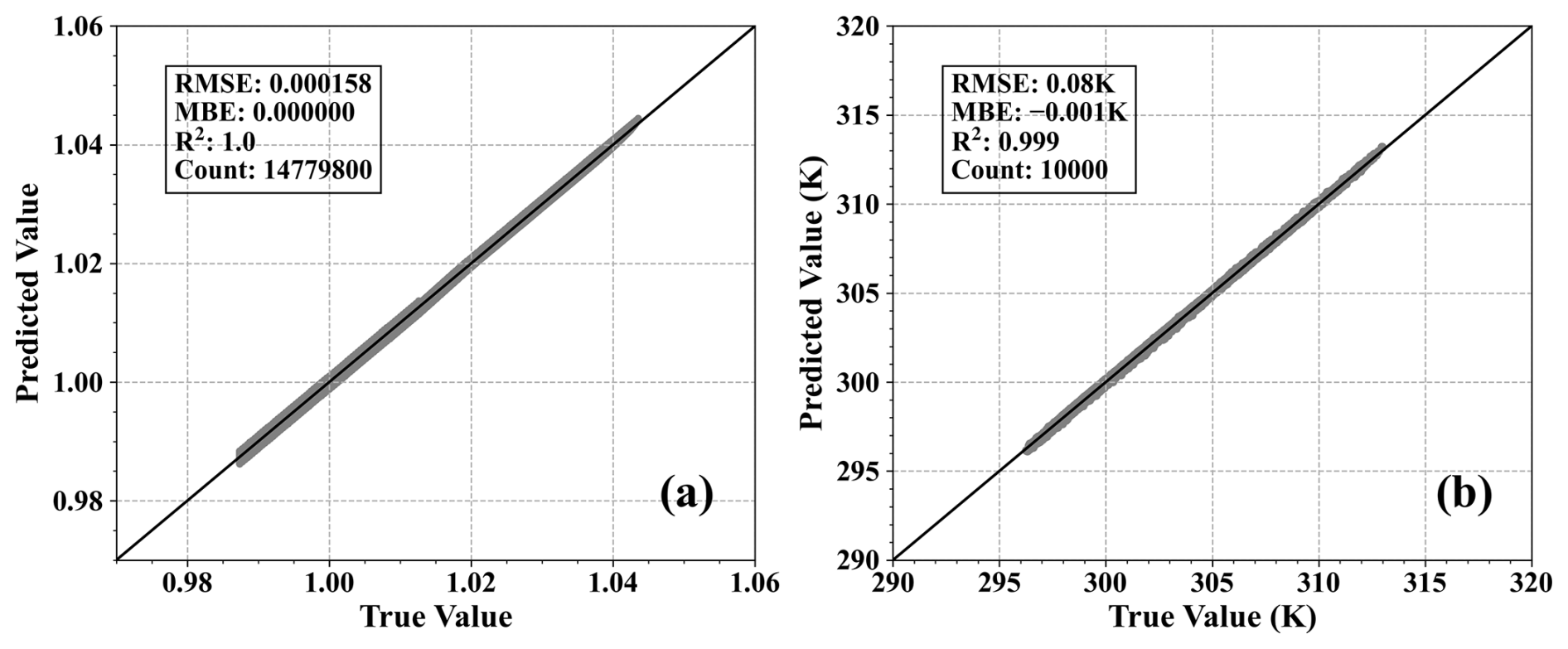
Figure A1 Performance of the polynomial fitting for (a) Φ and (b) T_hemi.

Appendix B

The sampling of label data is essential in the estimation of hypothetical clear-sky LST since the large volume of clear-sky LST observations. In this study, a representative sub-dataset was determined through a two-step sampling approach:

Step 1: determining the number of samples by evaluating the CatBoost model's performance in fitting the annual maximum LST (i.e., $T_{\max }=\mathrm{MAST}+\mathrm{YAST}$). Due to its highest level of heterogeneity, T_max is the most challenging variable for CatBoost to fit. Here, a CatBoost model was trained with the inputs of following features: Lat, Lon, LCT, CT, FVC, DEM, and the annual mean values of R_in, T_2 m, and D_2 m, as shown in Eq. (B1).

$$\begin{array}{}\text{(B1)}& \begin{array}{rl}{T}_{\max }=& f_{\mathrm{CatBoost}}\left(\mathrm{Lat},\mathrm{Lon},\mathrm{LCT},\mathrm{CT},\mathrm{FVC},\mathrm{DEM},R_{\mathrm{in}},\right.\\ & \left.T_{\mathrm{2}\mathrm{m}},D_{\mathrm{2}\mathrm{m}}\right)\end{array}\end{array}$$

Firstly, 10 % of the samples (974 403 samples) were used to tune the hyperparameters of the CatBoost model using a Bayesian optimization method. Another 30 % of the samples (2 923 400 samples) were allocated as the test set. The training set includes a total of 5 847 441 samples (i.e., 60 % of the samples). Aimed to determine the optimal sample size, directly transverse all the possible sample sizes over training set is impractical. In this study, the number of training samples was gradually increased from 2000 to 100 000 with an increment of 2000. As shown in Fig. B1a, the optimal sample size (i.e., 37 000) was determined based on the point at which the RMSE variation (i.e., $\left|\mathrm{\Delta }\mathrm{RMSE}\right|$) remained less than 0.001 K.

Step 2: determining the exact geolocations of 37 000 points for each year (i.e., 6 years from 2018 to 2023). Here, a conditioned Latin hypercube sampling (cLHS) method was employed, which first divides the features into equal partitions according to their values and then randomly selects sample points from each partition. It has been demonstrated to be both efficient and reliable for large datasets (Minasny and McBratney, 2006; Yang et al., 2020). The input features for this step are identical to those in Eq. (B1). The final spatial distribution of 37 000 selected points per year is shown in Fig. B1b–g, indicating a uniform distribution across the FY-4A disk without significant clustering.

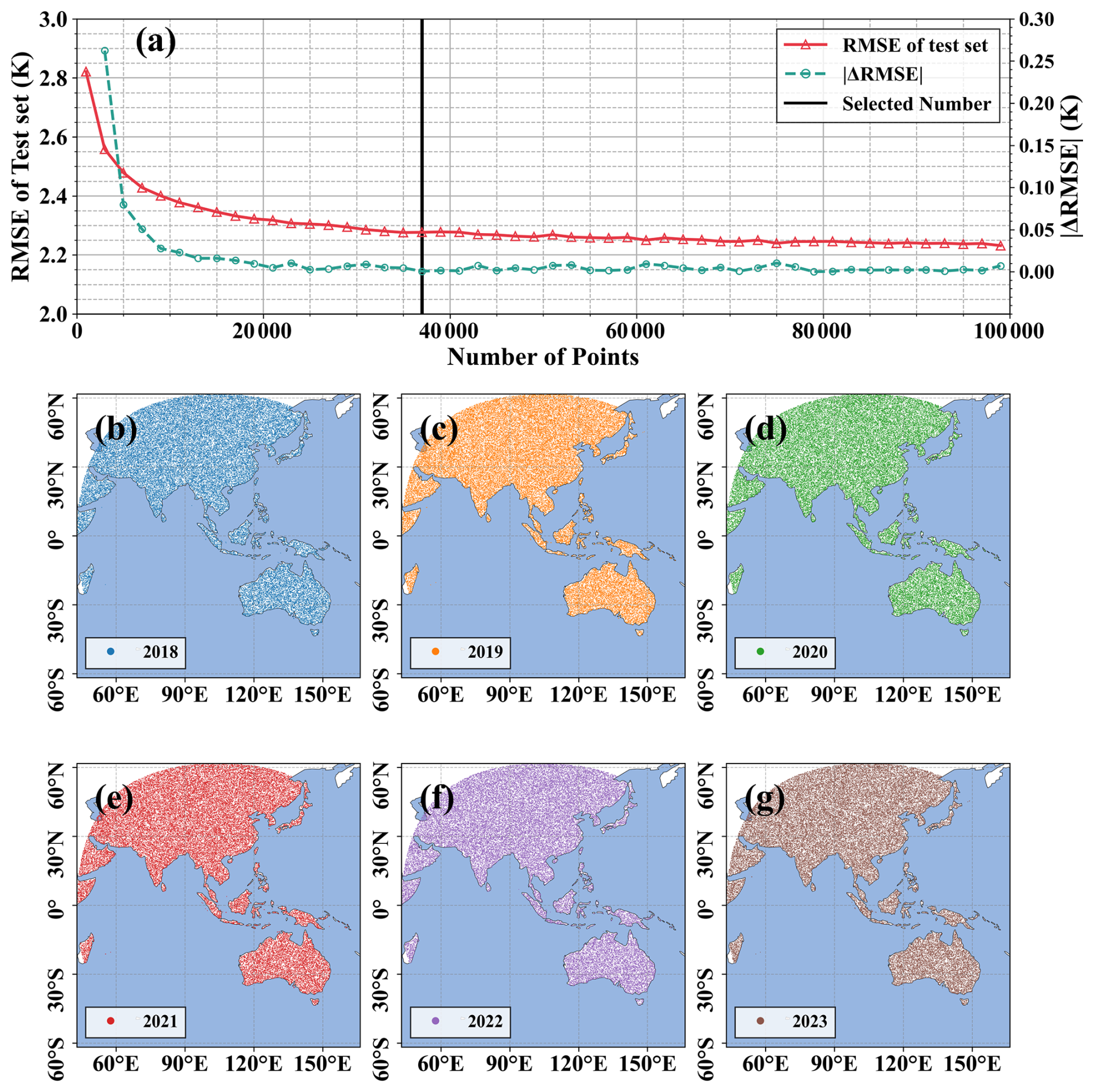
Figure B1 The selection of optimal sample number (a) and the geolocation of 37 000 sample points in (b) 2018, (c) 2019, (d) 2020, (e) 2021, (f) 2022, (g) 2023.