A global high-resolution temperature and salinity reconstruction by spatiotemporal multiscale correlations and dynamic height constraints

High-resolution temperature and salinity (T & S) gridded datasets are essential for exploring large and mesoscale ocean phenomena. In this study, a global, weekly T & S gridded dataset with a horizontal resolution of $\mathrm{1}/\mathrm{4}$° and a depth range of 0–1500 m from 2005 to 2023 is reconstructed using a four-dimensional multigrid analysis (4D-MGA) framework, based on the T & S profiles in WOD23. With minimal prior statistical assumptions, the 4D-MGA efficiently extracts information from in-situ T & S profiles and satellite-observed sea level anomalies by integrating multiscale spatiotemporal correlation and physical constraints. The results show that the 4D-MGA product successfully delivers a credible, high-resolution analysis that combines robustness with reliable mesoscale information. Specifically, our product exhibits a lower root mean square error and excellent unbiased performance on a global scale when compared with the ARMOR3D product and the GLORYS reanalysis. Furthermore, the clear recirculation in the western boundary currents (WBCs) can be well captured by the 4D-MGA product. The product is then applied to investigate the linear trends of geostrophic transport within five key sections in WBCs. The Kuroshio and Agulhas Current transports exhibit significant decreasing trends, with rates of 0.34 ± 0.07/0.26 ± 0.06, 0.23 ± 0.05/0.10 ± 0.06, and 0.30 ± 0.06/0.12 ± 0.05 Sv yr⁻¹ in 4D-MGA, ARMOR3D, and GLORYS, respectively. The weekly reconstructed dataset (4D-MGA) is freely available at https://doi.org/10.5281/zenodo.19378150 (Wu et al., 2026a).

1 Introduction

Temperature and salinity (T & S) are recognised as the two fundamental factors in the physical oceanography (Talley et al., 2011). Three-dimensional (3D) gridded T & S fields play a crucial role in studying multi-scale ocean dynamics (e.g., Zhang et al., 2014; Li et al., 2022; Miyaji et al., 2025; Zhou et al., 2025), optimizing ocean observations (e.g. Tan et al., 2023, 2025; Garcia et al., 2024; Reagan et al., 2024b), evaluating model performance (e.g., Tang et al., 2003; Matei et al., 2012; Polkova et al., 2023), as well as investigating climate change (e.g. Lyman and Johnson, 2014; Ishii et al., 2017; Bagnell and DeVries, 2021; Liang et al., 2021; Liu et al., 2026; Pan et al., 2026). The reconstruction of a global, high-quality 3D T & S fields remains a fundamental pursuit in the relevant literature.

Nowadays, three distinct types of 3D T & S products have been identified, namely the objective analysis, the reanalysis, and the artificial intelligence (AI) based products, according to the historical development of the subject. Objective analysis products were established through the spatiotemporal correlation of error distributions between observations and background fields (Roemmich and Gilson, 2009; Guinehut et al., 2012; Good et al., 2013; Gaillard et al., 2016; Cheng and Zhu, 2016; Li et al., 2017; Zhou et al., 2023). Reanalysis products utilize ocean numerical models to supply background information, and combine assimilation methods to link the observations and models to produce dynamically consistent T & S analyses (Forget et al., 2015; Chamberlain et al., 2021; Lellouche et al., 2021; Chepurin et al., 2025; De Boisseson et al., 2024). AI products have grown in recent years. They are based on learning the representative correlations among multiple input variables (e.g., Su et al., 2020; Tian et al., 2022; Zhu et al., 2025; Wang et al., 2026).

Each product possesses advantages and disadvantages. Reanalysis products are capable of representing continuous dynamical evolution with fine-scale structures (e.g., Mason et al., 2019; Castillo-Trujillo et al., 2023; El Aouni et al., 2025). Nonetheless, the model errors and parameterisation uncertainties will give rise to unrealistic results (e.g., Schneider et al., 2013; Paul et al., 2025). AI-based products offer powerful nonlinear fitting capabilities, but there are limitations in interpretability, the risk of perpetuating biases, and errors present in training data (Gray et al., 2024; Nunziante et al., 2025). In contrast, objective analysis products show lower performance in continuity and resolution, but can provide the most reliable representation of observations, with minimal errors (Chang et al., 2014; Carton et al., 2019). What's more, the heavy reliance on observations ensures a greater degree of determinism. They are often regarded as a reference benchmark for evaluations (e.g., Szekely, 2022; Cao et al., 2026), though their quality is dependent on the quantity and distribution of observations.

At present, the distribution of the in-situ T & S observations is uneven in terms of both space and time. Even for the largest global observation system, the spatial resolution of Argo is only ∼ 3° × 3° (Argo, 2026). Therefore, the present objective analysis products remain limited in capturing mesoscale signals due to their relatively low horizontal resolution (1° × 1°) (e.g., Roemmich and Gilson, 2009; Gaillard et al., 2016; Cheng and Zhu, 2016; Li et al., 2017), which hampers our understanding of the multi-scale oceanic dynamic processes. On the other hand, the satellite-based products feature relatively high spatiotemporal resolutions (e.g. Donlon et al., 2012; AVISO/DUACS, 2024), while they cannot provide subsurface information. It is still challenging to combine in-situ and satellite observations in objective analysis to create global, high-quality and high-resolution 3D gridded T & S fields.

The issue under consideration is the challenge of separating multi-scale superimposed signals and leveraging the spatiotemporal continuity and multivariate physical linkages in most objective analysis methods (e.g., Paris et al., 2002; Gray and Riser, 2015). On the other side of the spectrum, as a popular approach in data assimilation, four-dimensional variational (4D-Var; Le Dimet and Talagrand, 1986) uses an adjoint model to directly enforce temporal correlations and deterministic physical constraints. It has been proved that 4D-Var can generate dynamically consistent, mesoscale-resolving ocean estimates (e.g., Forget et al., 2015; Wang et al., 2022). A similar philosophy can be extended to objective analysis. The four-dimensional multigrid analysis (4D-MGA; Zhou et al., 2023, Wu et al., 2026b) features spatiotemporal evolution constraints and deterministic physical links without relying on prior statistical assumptions. Through the multigrid analysis (MGA; Li et al., 2008, 2013; Han et al., 2011, 2013), error signals in T & S fields are progressively distilled from large to small scales. Based on these advantages, 4D-MGA has been successfully used in reconstructing 3D gridded T & S fields in a regional ocean with a powerful ability to capture mesoscale signals (e.g., Zhou et al., 2023). Now it is time for us to use this excellent method to reconstruct a global high-resolution 3D gridded T & S field.

This study constructs a $\mathrm{1}/\mathrm{4}$° global subsurface (0–1500 m) T & S gridded dataset from 2005–2023 based on the 4D-MGA method. A comprehensive evaluation of the dataset is conducted. Furthermore, the detailed 3D structure and long-term trends of the transport of the western boundary currents (WBCs) were also investigated.

The remainder of this paper is organized as follows. Section 2 introduces the datasets and the 4D-MGA method employed in this study. The overall performance of our product is introduced in Sect. 3. Data availability is described in Sect. 5. Sections 4 and 6 provide conclusion and discussion.

2 Data and Methods

2.1 Data

2.1.1 Background Field

Weekly background fields of T, S and sea level anomaly (SLA) are required as prior inputs for the 4D-MGA. The $T/S$ background fields are derived from the high-resolution ($\mathrm{1}/\mathrm{4}$°) World Ocean Atlas 2023 (WOA23; Reagan et al., 2024a). To match our study period, we merged the available WOA23 decadal monthly fields (2005–2014 and 2015–2022) via time-span weighted averaging to generate a representative climatology. The SLA climatology was computed from daily AVISO SLA analysis (https://doi.org/10.48670/moi-00148, E.U. CMEMS, 2024) over the same period. All monthly climatological fields were linearly interpolated to the weekly analysis times, corresponding to the 4D-MGA product.

2.1.2 In-situ T & S Observations

In-situ T & S in standard levels were obtained from the World Ocean Database 23 (WOD23; Mishonov, 2024). The WOD23 aggregates global ocean observations from diverse platforms, including OSD, CTD, XBT, MBT, PFL, DRB, MRB, and GLD. WOD23 implements a well-established quality control (QC) system (Garcia et al., 2024). All observations failing to meet any of the WOD23 QC criteria were discarded. Systematic biases in XBT and MBT data were corrected according to the method of Cheng et al. (2014). Furthermore, an additional level of QC was conducted. Data were excluded where the errors relative to the background field exceeded three times the local error standard deviation (SD; Fig. S1 in the Supplement). This step removed ∼ 1 % of the profiles. In total, there are ∼ 4.67 × 10⁶ temperature and ∼ 4.32 × 10⁶ salinity profiles used in the study to conduct the objective analysis (Fig. S2).

In-situ T & S from EN4 (Good et al., 2013) was used as a reference to evaluate the performance of the 4D-MGA product. It collects and synthesizes profile observations from multiple sources, including Argo, WOD, and GTSPP, and applies further rigorous QC and data correction to each dataset. Only profiles with a QC flag of 1 (good) were utilised.

2.1.3 Tide Gauge Observations

The daily-averaged sea level data from the UHSLC tide gauges (Caldwell et al., 2015) were used as an independent reference for evaluating dynamic height anomalies (DHA). A total of 129 tide gauges covering 2005–2021 were selected for analysis (Fig. 4b). For all selected stations, both the tide gauge data and the DHA products were subjected to a process of time-mean value removal, with the objective of aligning them to a common reference level. Subsequently, a 12-week low-pass Gaussian filter is then applied to the tide gauge data to suppress high-frequency signals.

2.1.4 Blended Satellite-derived Products

Blended satellite-derived SLA products were ingested into 4D-MGA product as well. We employed the CMEMS AVISO Level-4 SLA analysis, which is the same dataset as that used to generate the climatological background field. The horizontal resolution of this product is $\mathrm{1}/\mathrm{8}$°. To improve computational efficiency, the AVISO SLA analysis were remapped onto the WOA23 horizontal grid.

The Ocean Surface Current Analyses Real-time (OSCAR; ESR, 2009) surface geostrophic current product was used for an independent reference for evaluation. OSCAR provides global $\mathrm{1}/\mathrm{4}$° geostrophic currents derived from satellite altimetry. In this study, the final level was used from 1 January 2005 to 5 August 2022, and the interim level from 6 August 2022 to 31 December 2023, as the final level ceased updates during the latter period.

2.1.5 Independent products for intercomparison

The ARMOR3D is a global 3D T & S product with a horizontal resolution of $\mathrm{1}/\mathrm{4}$°, covering depths from 0 to 5500 m (Guinehut et al., 2012). ARMOR3D uses a two-step approach to generate fine-scale T & S structures: first, it reconstructs preliminary 3D T & S fields from satellite-derived OSTIA SST (Nunes et al., 2012), AVISO SLA, and SMOS and SMAP sea surface salinity. This reconstruction is based on multivariate linear regression derived from historical in-situ profiles. Second, it further optimizes the reconstructed fields using real-time in-situ T & S observations. In this study, the multi-year reprocessed weekly data in ARMOR3D were used.

The GLORYS12V4 (hereinafter referred to as GLORYS) product (Lellouche et al., 2021) is a global eddy-resolving ocean reanalysis with a horizontal resolution of $\mathrm{1}/\mathrm{12}$°, spanning depths from 0.5 to 5728 m. GLORYS assimilates satellite observations including AVHRR SST, AVISO L3 SLA, CERSAT sea ice concentration (Ezraty et al., 2007), as well as in-situ T & S observations. In our study, the reprocessed daily data covering 2005–2021 were applied. In subsequent evaluations, these datasets were subsampled to a weekly frequency in order to align with the 4D-MGA product.

2.2 Reconstruction Methods

2.2.1 4D-MGA

Our reconstruction method adapts the 4D-MGA framework of Wu et al. (2026b). By introducing the Laplace operator (S), 4D-MGA can simultaneously define the spatiotemporal correlation of ocean variables. The 4D-MGA is aimed at addressing the analysis increments ($\stackrel{\mathrm{̃}}{\mathit{X}}$) relative to the background field (X^b). The cost function is

$$\begin{array}{}\text{(1)}& \begin{array}{rl}J\left(\stackrel{\mathrm{̃}}{\mathit{X}}\right)& ={\displaystyle \frac{\mathrm{1}}{\mathrm{2}}}{\stackrel{\mathrm{̃}}{\mathit{X}}}^T\left[\mathit{\alpha }\mathbf{S}\right]\stackrel{\mathrm{̃}}{\mathit{X}}+{\displaystyle \frac{\mathrm{1}}{\mathrm{2}}}{\left[\mathbf{H}\left({\mathit{X}}^{\mathrm{b}}+\stackrel{\mathrm{̃}}{\mathit{X}}\right)-{\mathit{Y}}^{\mathrm{obs}}\right]}^T\\ & \cdot {\mathbf{O}}^{-\mathrm{1}}\left[\mathbf{H}\left({\mathit{X}}^{\mathrm{b}}+\stackrel{\mathrm{̃}}{\mathit{X}}\right)-{\mathit{Y}}^{\mathrm{obs}}\right].\end{array}\end{array}$$

Where the first term on the right-hand side is the smoothing term based on the Laplace operator (S), α is the penalty coefficient matrix to define the weight of the smoothing term; the second term is the observation term, where Y^obs represents the observations, H represents the linear projection operator from the background to the observations, and O⁻¹ is the diagonal inverse matrix with elements of independent observation errors.

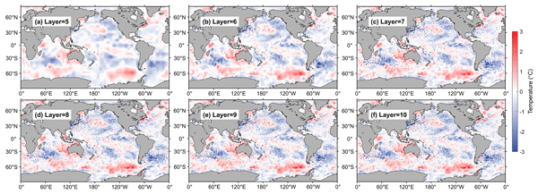
In Eq. (1), the smoothing term defines the continuity of error evolution, which represents minor, static constraints. The MGA method (Li et al., 2008, 2013; Han et al., 2011, 2013) is therefore employed to provide the dominant multi-scale spatiotemporal correlations. MGA allows for the extraction of observational signals sequentially from coarse to fine resolutions. After applying Eq. (1) on the nth grid layer, the analysis results will be projected onto the n+1th grid layer by grid-doubling. As shown in Fig. 1, the coarse grid layers extract a smoothed large-scale signal from observations, while the fine grid layers complement the small-scale structures. By summing the analysis fields from each layer, the final mapping result (X^a) is obtained:

$$\begin{array}{}\text{(2)}& {\mathit{X}}^{\mathrm{a}}={\mathit{X}}^{\mathrm{b}}+\sum _{n=N_{\mathrm{start}}}^{N_{\mathrm{end}}}{\mathbf{P}}^{\left(n\right)}{\stackrel{\mathrm{̃}}{\mathit{X}}}^{\left(n\right)}.\end{array}$$

Where N_start and N_end are the first and last layers of the grid, respectively; P⁽ⁿ⁾ is the projection matrix interpolated from the nth layer grid to the background grid, and ${\stackrel{\mathrm{̃}}{\mathit{X}}}^{\left(n\right)}$ is the increment of the observation relative to the background at the nth layer.

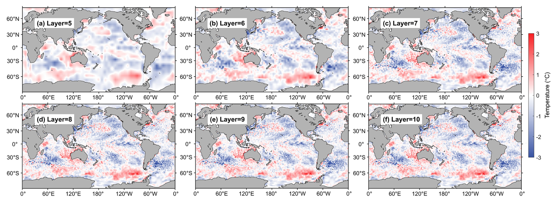
Figure 1 Schematic of cumulative adjustments to sea surface temperature (SST) relative to WOA23, shown sequentially from the 5th to the 10th layers of the 4D-MGA procedure.

However, in regions with sparse observations, the coarse grid layers may generate unrealistically long-range correlations. A pseudo-observation scheme is therefore introduced to constrain this effect, with its specific configuration following Wu et al. (2026b).

2.2.2 Dynamic height integration

In the 4D-MGA framework, AVISO SLA analysis will be combined with $T/S$ observations. SLA will be approximated as the DHA. Since high-frequency barotropic signals induced by wind forcing and the inverse-barometer effect have been removed in the Level-4 SLA analysis, the barotropic component can be neglected. Through dynamic height integration, a direct relationship between T & S and the perturbation in DHA (denoted as δDHA) can then be established as follows:

$$\begin{array}{}\text{(3)}& \mathit{\delta }\mathrm{DHA}=-\underset{\mathrm{0}}{\overset{z_m}{\int }}{\displaystyle \frac{\mathit{\rho }\left(P,T,S\right)-\mathit{\rho }\left(P,T^{\mathrm{b}},S^{\mathrm{b}}\right)}{\mathit{\rho }\left(P,T^{\mathrm{b}},S^{\mathrm{b}}\right)}}\mathrm{d}z.\end{array}$$

Where ρ is the seawater density; z_m=1500 m is the reference depth. If the water depth is less than z_m, the SLA observations at that grid point are not considered; T^b and S^b are background fields of T & S, respectively. P=ρ₀gz is the approximate pressure, where g (9.8 m s⁻²) is the gravitational acceleration and ρ₀ (1025 kg m⁻³) denotes the reference density.

By incorporating Eq. (3), the observation term for a single SLA observation can be derived:

$$\begin{array}{}\text{(4)}& \begin{array}{rl}\mathrm{OBS}\left(\stackrel{\mathrm{̃}}{\mathit{T}},\stackrel{\mathrm{̃}}{\mathit{S}}\right)& ={\displaystyle \frac{\mathrm{1}}{\mathrm{2}}}[\mathbf{H}\mathit{\delta }\mathrm{DHA}\left({\mathit{T}}^{\mathrm{b}}+\stackrel{\mathrm{̃}}{\mathit{T}},{\mathit{S}}^{\mathrm{b}}+\stackrel{\mathrm{̃}}{\mathit{S}},{\mathit{T}}^{\mathrm{b}},{\mathit{S}}^{\mathrm{b}}\right)-\mathit{\delta }{Y}_{\mathrm{sla}}{]}^T\\ & O^{-\mathrm{1}}\left[\mathbf{H}\mathit{\delta }\mathrm{DHA}\left({\mathit{T}}^{\mathrm{b}}+\stackrel{\mathrm{̃}}{\mathit{T}},{\mathit{S}}^{\mathrm{b}}+\stackrel{\mathrm{̃}}{\mathit{S}},{\mathit{T}}^{\mathrm{b}},{\mathit{S}}^{\mathrm{b}}\right)-\mathit{\delta }{Y}_{\mathrm{sla}}\right].\end{array}\end{array}$$

Where $\stackrel{\mathrm{̃}}{\mathit{T}}$ and $\stackrel{\mathrm{̃}}{\mathit{S}}$ represent the increments of the background field of T & S from the surface to z_m, respectively; Y_sla is the observations of SLA and O is the observation error.

Note that Eq. (4) characterizes an underdetermined mapping between AVISO SLA analysis and the full-depth vertical T & S profiles. During the minimization process, the solver tends to adjust the DHA via the highest-gradient elements, specifically S at deep layers. To mitigate this inconsistency with physical reality, α is prescribed based on the variable and vertical resolution (Wu et al., 2026b).

2.3 Production of the weekly data

As shown in Eq. (1), the 4D-MGA method generates four-dimensional analysis increments relative to the background fields. Following the approach of Zhou et al. (2023) and Wu et al. (2026b), the central time increments are selected to reconstruct the analysis field. In this study, the minimization time window (MTW) was set to 120 d. The finest vertical layer was divided into the following 33 levels: 0.0, 2.5, 7.5, 12.5, 17.5, 22.5, 27.5, 32.5, 37.5, 42.5, 47.5, 52.5, 57.5, 62.5, 67.5, 72.5, 77.5, 82.5, 87.5, 92.5, 97.5, 112.5, 137.5, 187.5, 212.5, 237.5, 262.5, 287.5, 387.5, 487.5, 675.0, 1075.0, and 1500.0 m. The MGA was performed sequentially from a horizontal resolution of ∼ 7° (with 3 vertical grid layers and 2 temporal layers) to a resolution of ∼ $\mathrm{1}/\mathrm{4}$° (with 33 vertical layers and 5 temporal layers distributed over the MTW). For satellite observations, whose data density is sufficient, only observations at the analysis time were combined. A weekly analysis was conducted from 1 January 2005, to 30 December 2023, yielding a total of 992 reconstructions.

2.4 RMSE, bias and ACC

To estimate the performance of 4D-MGA, we introduce the root mean square error (RMSE), bias, and anomaly correlation coefficient (ACC) as validation metrics, with their respective formulas given as follows:

$$\begin{array}{}\text{(5)}& {\displaystyle }\mathrm{RMSE}=\sqrt{{\displaystyle \frac{\mathrm{1}}{n}}\sum _{i=\mathrm{1}}^n{\left(X_i-Y_i\right)}^{\mathrm{2}}},\text{(6)}& {\displaystyle }\mathrm{bias}={\displaystyle \frac{\mathrm{1}}{n}}\sum _{i=\mathrm{1}}^n\left(X_i-Y_i\right),\text{(7)}& {\displaystyle }\mathrm{ACC}={\displaystyle \frac{\mathrm{cov}\left(\stackrel{\mathrm{̃}}{\mathit{X},}\stackrel{\mathrm{̃}}{\mathit{Y}}\right)}{\mathit{\sigma }\left(\stackrel{\mathrm{̃}}{\mathit{X}}\right)\mathit{\sigma }\left(\stackrel{\mathrm{̃}}{\mathit{Y}}\right)}}.\end{array}$$

Where X_i denotes the gridded dataset and Y_i is the reference data (including in-situ and satellite derived datasets), with $\stackrel{\mathrm{̃}}{\mathit{X},}\stackrel{\mathrm{̃}}{\mathit{Y}}$ representing their respective anomalies. Here, cov stands for covariance and σ is the SD.

2.5 Calculation of the geostrophic currents

The geostrophic currents are estimated by using the thermal wind relation referenced to the 1500 m level:

$$\begin{array}{}\text{(8)}& \left\{\begin{array}{l}{u}_{\mathrm{g}}\left(x,y,z\right)=\frac{g}{f{\mathit{\rho }}_{\mathrm{0}}}\underset{z=\mathrm{1500}\mathrm{m}}{\overset{z}{\int }}\frac{\partial }{\partial y}\mathit{\rho }\left(x,y,z\right)\mathrm{d}z\\ v_{\mathrm{g}}\left(x,y,z\right)=-\frac{g}{f{\mathit{\rho }}_{\mathrm{0}}}\underset{z=\mathrm{1500}\mathrm{m}}{\overset{z}{\int }}\frac{\partial }{\partial x}\mathit{\rho }\left(x,y,z\right)\mathrm{d}z\end{array}.\right.\end{array}$$

Where $u_{\mathrm{g}}\left(x,y,z\right)$ and $v_{\mathrm{g}}\left(x,y,z\right)$ are the zonal and meridional geostrophic velocity components, respectively; f is the Coriolis parameter; and x, y, z denote the zonal, meridional, and vertical coordinates, respectively.

3 Results

3.1 T & S errors

To evaluate the overall reconstruction performance, a comparison is made between the RMSE of the 4D-MGA product and that of the ARMOR3D and GLORYS, using EN4 observations as a reference. Figure 2 shows the spatially binned RMSE of T & S for the three products.

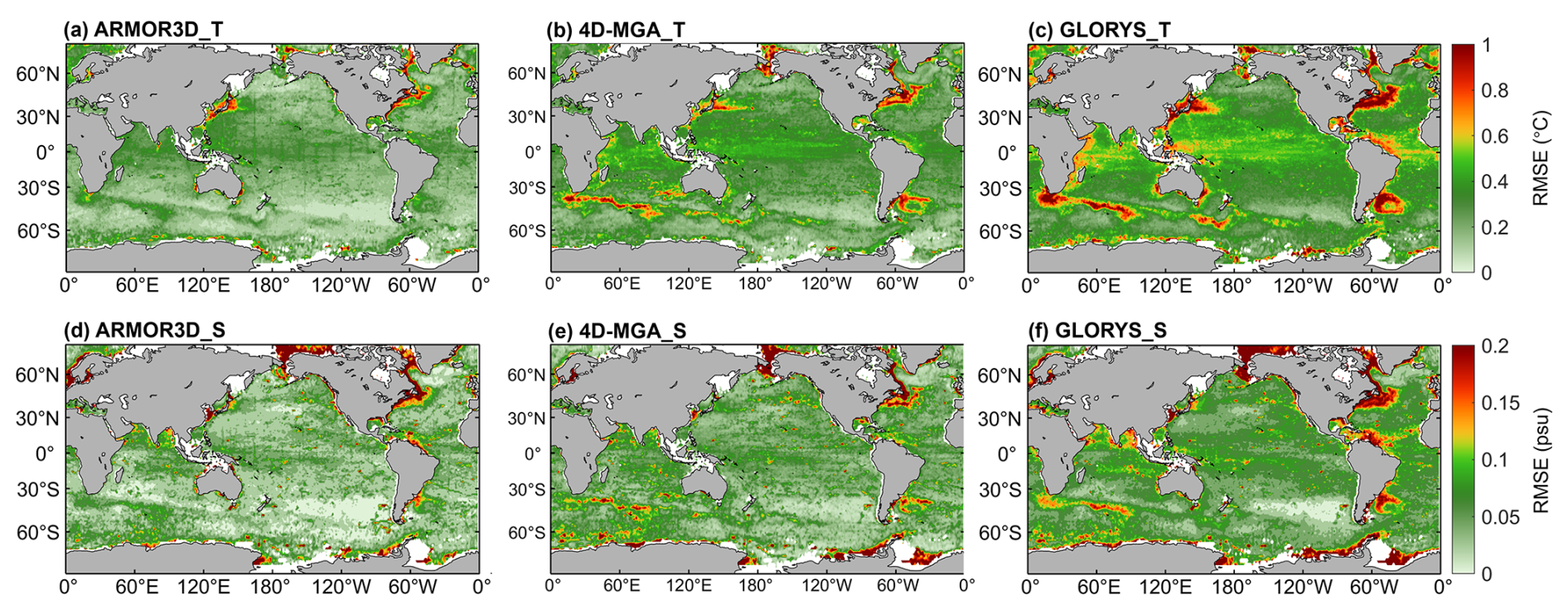
Figure 2 Spatial distribution of the RMSE averaged over 1° × 1° bins, the full water column (0–1500 m), and the entire period for ARMOR3D temperature (a), 4D-MGA temperature (b), and GLORYS temperature (c). Panels (d)–(f) are the same as (a)–(c), but for salinity.

The RMSE of 4D-MGA has been shown to be comparable to those of GLORYS and ARMOR3D. Globally averaged $T/S$ RMSE values are 0.29 °C/0.08 psu, 0.49 °C/0.12 psu, and 0.33 °C/0.07 psu for ARMOR3D, GLORYS, and 4D-MGA, respectively. Regions of higher errors are primarily located in the WBCs, the equatorial zone, and the Antarctic Circumpolar Current where active multi-scale dynamics are prevalent (e.g., Figs. 5–6 below). Furthermore, the relatively large errors are manifested in the marginal seas, coastal ocean, and high latitudes, which are presumably associated with the relatively sparse observations in these regions (e.g., Fig. S2). In terms of extreme errors, the percentage of grid points with $T/S$ RMSE exceeding 0.5 °C/0.1 psu is 7 %/18 % for ARMOR3D, 33 %/31 % for GLORYS, and 13 %/14 % for 4D-MGA.

The vertical structure of the error is further examined. As shown in Fig. 3a, 4D-MGA achieves a reasonably low average T & S RMSE across all vertical layers. The maximum T RMSE in the vertical are 0.48 °C (ARMOR3D), 0.67 °C (GLORYS), and 0.49 °C (4D-MGA). For S (Fig. 3b), 4D-MGA exhibits relatively lower RMSE in the upper ocean (< 300 m), with the maximum RMSE of 0.12 psu.

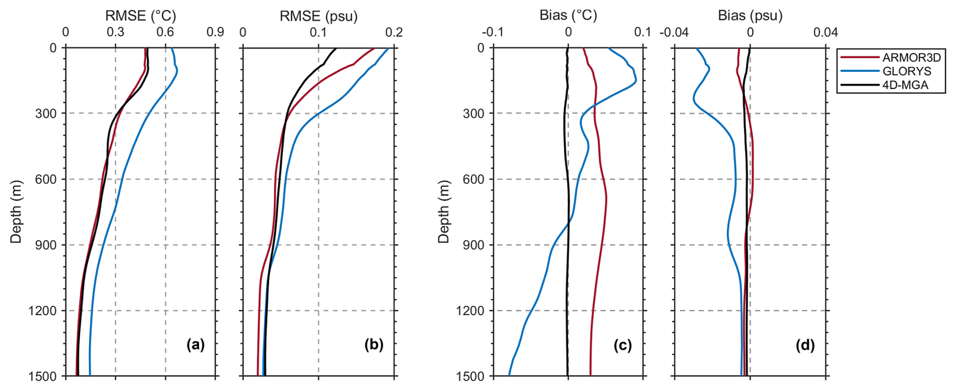
Figure 3 Full-period horizontal averages (smoothed using a moving average) of RMSE (a, b) and bias (c, d) for temperature (a, c) and salinity (b, d) from ARMOR3D, GLORYS, and 4D-MGA.

The favourable RMSE performance of 4D-MGA in Fig. 3a and b can be largely attributed to its exceptional bias control (Fig. 3c and d). This bias advantage is further confirmed by the independent tests in Sect. 4.1 below. The coarse-resolution grid layers of 4D-MGA are sufficiently constrained by the available observational resolution, allowing them to converge robustly while filtering out small-scale random noise.

3.2 Dynamic height anomaly

Based on the gridded T & S, we further validate the performance of DHA from the 4D-MGA product. A case from 10 August 2013 was randomly selected and is shown in Fig. 4a–b. The distribution of DHA in 4D-MGA agrees well with the SLA in satellite observations. Both show rich mesoscale information (e.g., eddies, meanders and fronts etc.) with alternating positive and negative SLA in the WBCs and the Antarctic Circumpolar Current (Fig. 4a–b). In addition, it can be seen that the RMSE of DHA remains below 0.05 m in most regions. The relatively large (> 0.1 m) RMSEs appear in marginal seas, WBCs, Antarctic Circumpolar Current, and high latitudes (Fig. 4c), consistent with that in Fig. 2. At the same time, the ACC exceeds 0.6 over nearly the entire global ocean (Fig. 4d), with a distribution consistent with that of RMSE.

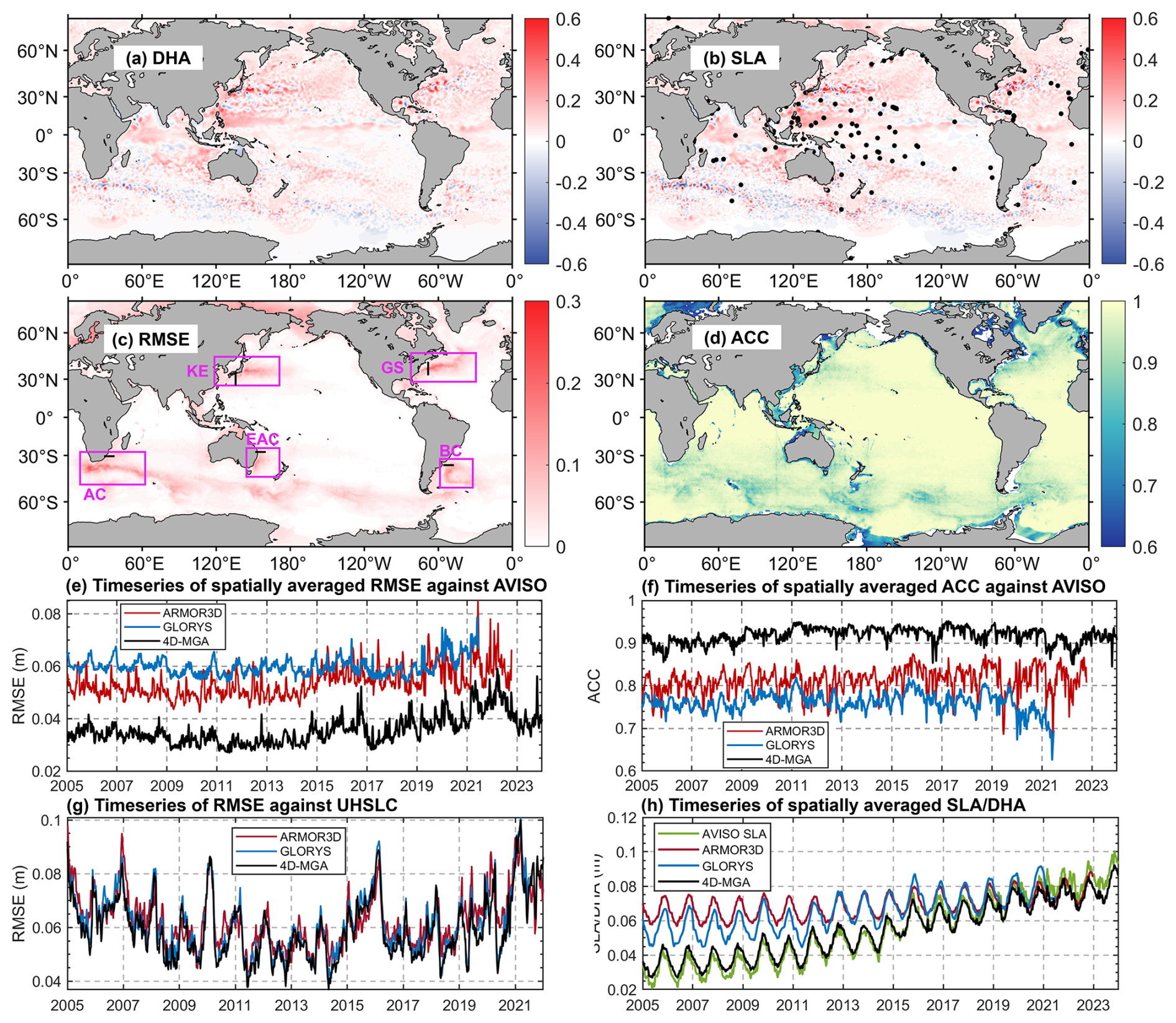
Figure 4 Spatial distribution of DHA (m) from the 4D-MGA product (a) and AVISO SLA analysis (m) (b) on 10 August 2013. Black dots in (b) indicate tide gauge stations. (c, d) Time-averaged RMSE (c) and ACC (d) of 4D-MGA DHA against AVISO SLA analysis. The pink boxes in (c) indicate the major WBC regions: Kuroshio Extension (KE), Gulf Stream (GS), Agulhas Current (AC), East Australia Current (EAC), and Brazil Current (BC). The black lines denote the WBC sections shown in Figs. 7–8. (e–g) Timeseries of spatially averaged RMSE (e), ACC (f), and SLA (AVISO) and DHA (ARMOR3D, GLORYS, and 4D-MGA) (g). (h) Timeseries of the RMSE relative to sea level from UHSLC tide gauges.

The timeseries of the DHA is also evaluated (Fig. 4e–h). As shown in Fig. 4e–f, 4D-MGA exhibits a significantly lower RMSE with a time-averaged value of 0.04 m (0.06 m in GLORYS and 0.05 m in ARMOR3D), and a higher ACC (time-averaged value of 0.91) over the entire period, compared with those of the GLORYS (time-averaged ACC of 0.76) and ARMOR3D (time-averaged ACC of 0.81). It is consistent with the relatively larger RMSE of GLORYS and ARMOR3D shown in Fig. 3. After 2014, an increase in RMSE alongside stronger temporal fluctuations appears, which coincides with variability of SLA (Fig. S3). This may be related to progressive upgrades in the AVISO SLA analysis' data fusion algorithms and the expanding constellation of altimeter missions (Pujol et al., 2016; Taburet et al., 2019). By contrast, the tide gauge evaluation shows little difference among the three products, all achieving a time-averaged RMSE of about 0.06 m (Fig. 4h). The DHA derived from 4D-MGA are consistent with the independent tide gauge observations, demonstrating its reliability.

The timeseries of the spatially averaged DHA estimated by the three products and AVISO SLA analysis show the pronounced interannual signals (Fig. 4g). Their distinct correlations (r=0.99, P<0.01 for 4D-MGA; r=0.79, P<0.01 for ARMOR3D; r=0.91, P<0.01 for GLORYS) with satellite observation show the advantage of the 4D-MGA product. In addition, the spatially averaged DHA of ARMOR3D and GLORYS significantly exceeds SLA about 2–3 cm before 2015. This is probably because their relatively large T & S biases (Fig. 3c–d) lead to a systematic overestimation. In contrast, 4D-MGA's DHA agrees well with the AVISO SLA analysis, showing the reliability of the 4D-MGA product.

3.3 Geostrophic currents

The surface geostrophic currents in WBC regions (the Kuroshio, the Gulf Stream, the Agulhas Current, the East Australia Current (EAC) and Brazil Current) for August 2013 are further evaluated (Figs. 5–6). It is evident that all of the products display the significant features of WBCs with the magnitude of the geostrophic current exceeding 0.5 m s⁻¹. The location, width and intensity of the WBCs are generally consistent with each other. Furthermore, the meanders, mesoscale eddies, and fronts with horizontal scale of 25–200 km are enriched in these regions, indicating the presence of active meso-scale dynamic features. Their structures and scales are also in line with OSCAR. For example, one mesoscale eddy is located at 32° N, 145° E in the south of the Kuroshio Extension in the 4D-MGA product (Fig. 5a). This eddy has a similar intensity (∼ 0.9 m s⁻¹) and radius (∼ 100 km) to those in the OSCAR (Fig. 5j). It is evident that the surface geostrophic current speeds estimated by the three products are smaller than those in satellite observations. One possible cause is the assumption of a motionless plane at 1500 m. However, the spatial patterns and magnitudes of the geostrophic current speeds demonstrate a high degree of agreement, despite the presence of certain discrepancies in detail. These discrepancies in WBCs are further quantified and compared with each other, with the time-averaged ACC/RMSE values of 0.81/0.12 m s⁻¹ for ARMOR3D, 0.69/0.16 m s⁻¹ for GLORYS, and 0.77/0.15 m s⁻¹ for 4D-MGA against OSCAR (Fig. 6i–j).

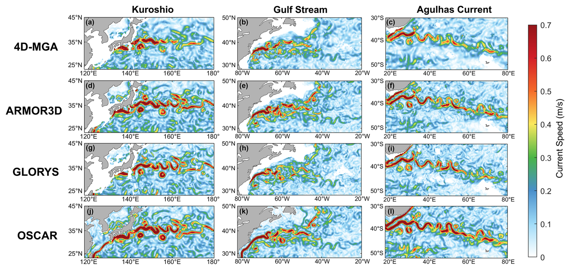
Figure 5 Spatial distribution of geostrophic current speed in selected WBC regions in August 2013. The weekly geostrophic currents from (a–c) 4D-MGA, (d–f) ARMOR3D, (g–i) GLORYS and (j–l) OSCAR are each weighted and averaged to form the monthly mean fields.

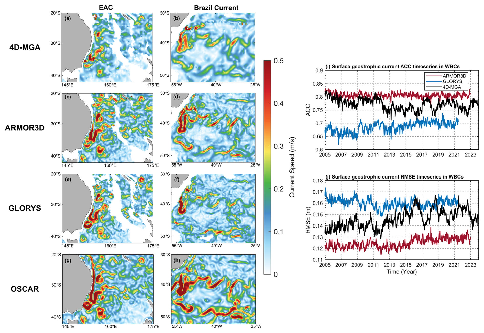
Figure 6 (a–h) Same as Fig. 5, but for the EAC and BC. (i, j) Timeseries of spatially averaged ACC (i) and RMSE (j) for surface geostrophic currents in the WBCs against OSCAR.

As demonstrated in Fig. 7, the main axis of the WBCs at the selected positions can be well captured from surface to deep ocean (> 1000 m), with their maximal (minimal) velocities of 0.53, 0.61, −0.23, −0.22, −0.21 m s⁻¹, respectively in Kuroshio, Gulf Stream, Agulhas Current, EAC, and Brazil Current. In addition, the key recirculation features in the WBCs can be adequately exhibited. For instance, the Kuroshio Counter Current (Fig. 7a), the southern recirculation of the Gulf Stream (Fig. 7b), the northward parts of the Agulhas anticyclonic circulation (Fig. 7c), and the northward recirculation of the EAC and Brazil Current (Fig. 7d–e). The location, structure and intensity of these recirculation have been shown to be consistent with previous findings (e.g., Imawaki et al., 2013; Sloyan et al., 2016; Zilberman et al., 2018; Chidichimo et al., 2021; Kawakami et al., 2022; Guo et al., 2024). Li et al. (2026) provided a comprehensive analysis of the recirculation features observed in WBCs, and these features cannot be captured by the low horizontal resolution (∼ 1°) data. Compared with ARMOR3D and GLORYS, the 4D-MGA product shows similar velocity distribution patterns across the five WBC sections, albeit with slightly weaker intensities (Figs. S4 and S5). The timeseries of globally averaged geostrophic currents in the vertical are further investigated, with all products in good agreement with each other (Fig. S6).

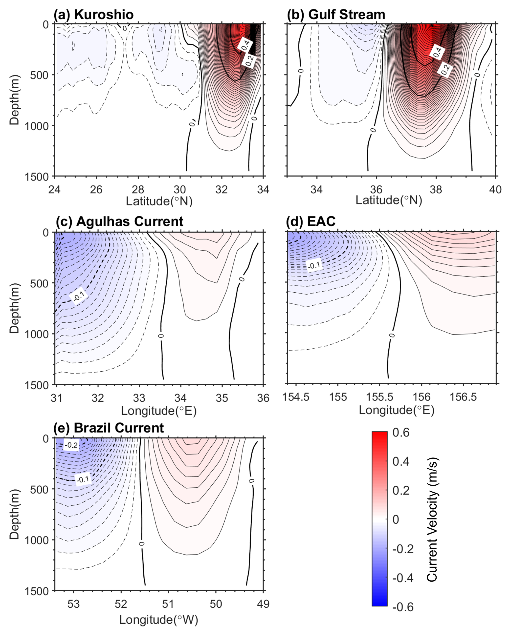
Figure 7 Climatological (2005–2023) geographic velocity sections in WBC sections from the 4D-MGA product. The contour interval is 0.01 m s⁻¹ of the Kuroshio (a) at 137° E, the Gulf Stream (b) at 68.5° W, the Agulhas Current (c) at 31° S, the EAC (d) at 27° S and the Brazil Current (e) at 37° S. The positive values in (a) and (b) represent the eastward currents, while they represent the northward currents in (c), (d) and (e).

3.4 The linear trends of geostrophic transports in WBCs

According to the geostrophic currents at each section in Fig. 7, the timeseries of the corresponding geostrophic transports can be estimated (Fig. 8). The linear trends of the geostrophic transports in WBCs vary with region. The northward geostrophic transport of the Kuroshio at 137° E and southward geostrophic transport of Agulhas Current at 31° S exhibit a marked and consistent decrease, with a trend of 0.34 ± 0.07/0.26 ± 0.06, 0.23 ± 0.05/0.10 ± 0.06, 0.30 ± 0.06/0.12 ± 0.05 Sv (1 Sv = 10⁶ m³ s⁻¹) per year in 4D-MGA, ARMOR3D, GLORYS products, respectively. The decreasing trend of the Kuroshio transports has been demonstrated in previous studies (e.g., Chandler et al., 2022; Guo et al., 2023), although it seems to be inconsistent with that in climate models (e.g., Yang et al., 2016; Chen et al., 2019). In contrast, trends for the geostrophic transports in other WBCs show less consistency across different products. In the Gulf Stream at 68.5° W, 4D-MGA product indicates a significant (P<0.01) positive trend of 0.39 ± 0.06 Sv per year, while other products show negative trends. Chi et al. (2021) have reported a slight increasing trend of the surface geostrophic transports of the Gulf Stream at the similar location during 1993 to 2018. Due to the reduction of the Atlantic Meridional Overturning Circulation (e.g., Yang et al., 2016; Weijer et al., 2020), the Gulf Stream was weakened over the past decades (Piecuch and Beal, 2023). Our estimated increase in Gulf Stream transport should be further investigated. The EAC at 27.5° S shows a pronounced decreasing trend of southward geostrophic transport for the 4D-MGA product, with a decrease of 0.20 ± 0.04 Sv per year. On the other hand, the Brazil Current shows nonsignificant trend of decrease of geostrophic transport for the 4D-MGA product. However, it shows an interesting interannual variability, which is probably linked to ENSO and wind stress curl as reported by De Paula et al. (2025).

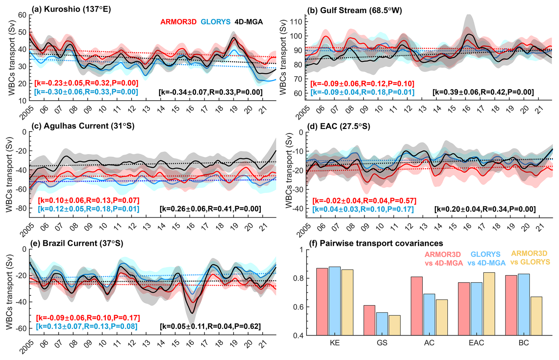
Figure 8 (a–e) Timeseries of the geostrophic transport in WBC sections. Northward and eastward velocities are defined as positive. The solid lines denote the monthly mean, the shaded areas ± 1 standard deviation, and the dashed lines the linear trend. The parameters k, R and P denote the slope of the linear trend (in Sv per year, with standard error), the linear correlation coefficient between the linear trend and the mean anomaly, and the significance level (p-value) of the linear trend, respectively. (f) Pairwise correlation coefficients of the monthly mean geostrophic transport.

Notably, our geostrophic transport estimates and trends discussed in the WBCs are probably contingent on the selected sections. Despite the presence of discrepancies among the estimates for different products, there is a high degree of consistency in their interannual variability. The correlation coefficient of the geostrophic transport between different products ranges from 0.86 to 0.88 for the Kuroshio, from 0.54 to 0.61 for the Gulf Stream, from 0.65 to 0.81 for the Agulhas Current, from 0.77 to 0.84 for the EAC, from 0.67 to 0.83 for the Brazil Current at the selected sections in our study (Fig. 8f). This demonstrates consistency among the products.

4 Discussion

4.1 The independent test

Our preceding assessments have validated the T & S against the EN4, which has overlapping observations with our ingested data. Hence, the generalization performance of the 4D-MGA method remains to be verified for further assessing the product's reliability. By randomly sampling 30 % and 60 % of the in-situ profiles in each MTW, we conducted independent tests for all analysis time steps in 2005–2023 (Fig. 9). In these independent tests, the observations included only $T/S$ profiles and the AVISO SLA analysis.

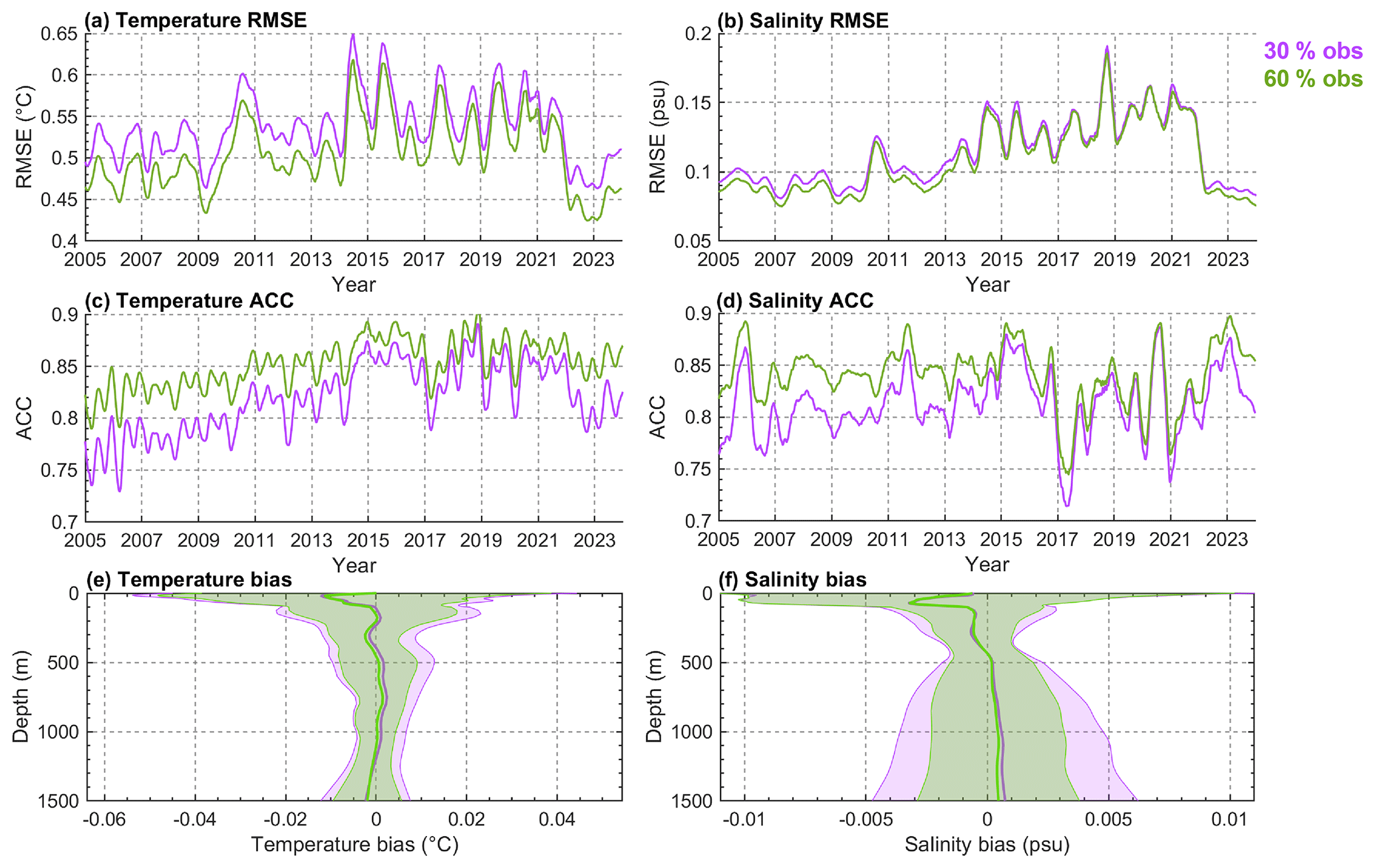
Figure 9 (a–d) Time series of RMSE and ACC relative to independent observations. (e, f) Vertical profiles of T & S bias from the independent tests, solid line indicates the mean bias, and the shaded area represents ± 1 SD.

To remove subgrid-scale noise in the in-situ observations for validation, we applied the filtering method from Huang et al. (2025). The filtering aims to align the SD of the observations with that of the product, which is 1.03 °C/0.20 psu at the observation locations. Consequently, we applied the filter to reduce the raw observational SD from 1.22 °C/0.24 psu to 0.88 °C/0.16 psu.

The results show 4D-MGA's excellent robustness. The method can effectively extract core dynamic signals from both small subsets and data-rich environments. Even with only 30 % of the in-situ observations, the ACC for T & S still exceeds 0.7, and the averaged RMSEs for T & S are smaller than 0.54 °C and 0.11 psu, respectively. Furthermore, as the observation density increases (Fig. S2), the ACC consistently improves, while the RMSE shows a slight increase. Complementing this robustness, the negligibly small mean and SD of the systematic bias further validate its excellent bias-correction capability (Fig. 9e–f).

4.2 Deficiencies and future improvements

While the 4D-MGA method and product demonstrate significant advantages and robust performance, the current analysis framework has several notable limitations. First, the use of SLA as a proxy for DHA introduces errors due to the omission of barotropic signals, especially in barotropic-dominated regions like the polar oceans and coastal zones. When combined with the optimization algorithm's gradient-seeking behaviour, this approximation error tends to cause distorted deep-layer adjustments. Second, due to computational constraints (Wu et al., 2026b), the temporal grid resolution used in this study is coarse (30 d). The limited number of temporal layers may not only filter out resolvable signals but also introduce additional noise. Third, due to the distribution and resolution of in-situ profiles, as well as the inherent smoothing of the analysis method, the effective resolution of the product is lower than its nominal grid resolution (Reynolds et al., 2013).

To address these limitations, several potential avenues are worth exploring in future research: (1) Incorporate bottom pressure data to separate barotropic and baroclinic signals (Li et al., 2025). Despite low accuracy and coarse resolution in current pressure datasets (Schindelegger et al., 2021; Chen et al., 2023; Yang et al., 2025), combining this method with in-situ constraints can refine dynamic height integration accuracy. (2) Refine the spatial scale and weighting of AVISO SLA analysis based on local in-situ data density to enhance the product's determinism. (3) Parallelize the minimizer to overcome array-size constraints. This would achieve a higher effective time resolution and better capture nonlinear evolutions. (4) Incorporate more physical constraints or data-driven approaches to recover small-scale information and compensate for the reduced effective resolution.

5 Data availability

The 4D-MGA product is freely available at https://doi.org/10.5281/zenodo.19378150 (Wu et al., 2026a). Here we provide a global ocean temperature and salinity gridded product at $\mathrm{1}/\mathrm{4}$° resolution on 57 vertical levels from 0–1500 m and at a weekly resolution from 2005 to 2023.

6 Conclusion

This study produced a weekly $\mathrm{1}/\mathrm{4}$° global subsurface T & S gridded dataset from 2005 to 2023 using the 4D-MGA method. Without prior statistical assumptions, the 4D-MGA efficiently extracts observational information via four-dimensional multi-scale analysis and physical constraints from dynamic height integration. Spatiotemporal correlations and multi-variable observational constraints enable the resolution of both large- and mesoscale structures. The results demonstrate that the 4D-MGA product performs well in several areas:

1. High accuracies. The 4D-MGA product achieves remarkably low RMSEs and biases relative to EN4. The time-averaged $T/S$ RMSE are 0.41 °C/0.08 psu, while the time-averaged absolute bias is 0.01 °C/0.01 psu.

2. Excellent ability to capture mesoscale information. Compared with the time-series of the eddy-resolved SLA in satellite observations, the global averaged DHA estimated by the 4D-MGA T & S gridded data set has a much lower RMSE, higher ACC and higher correlation coefficients (RMSE = 0.04 m; ACC = 0.89; r = 0.99, P<0.01). It is slightly better than that of the GLORYS (RMSE = 0.06 m; ACC = 0.76; r=0.91, P<0.01) and the ARMOR3D (RMSE = 0.05 m; ACC = 0.81; r=0.79, P<0.01). Moreover, the WBC structures (like eddies and recirculation) can also be accurately represented. This capability is further evidenced by its successful capture of long-term trends and interannual variability in WBC transports.

In summary, the 4D-MGA product provides a high-fidelity objective analysis dataset with considerable value for further understanding the oceanic mesoscale processes and climate change.