A year-long eddy covariance dataset over an Alpine Steppe on the central Tibetan Plateau: a landscape perspective on carbon and energy fluxes

The Tibetan Plateau (TP) is warming rapidly, with future projections suggesting continued warming that may amplify climate–carbon feedbacks. However, sparse in-situ observations and pronounced spatial heterogeneity in vegetation, soil moisture, and climate have limited our understanding of these ecosystem responses. Here, we present a continuous record of carbon and energy fluxes measured at a landscape scale (∼30 ha (0.3 km²)) in an alpine steppe ecosystem on the TP from July 2018 to June 2019. The dataset yields a cumulative net ecosystem exchange (NEE) of $-\mathrm{12.6}\pm \mathrm{16.4}$ g C m⁻², indicating a near carbon-neutral budget. Flux measurements were quality-filtered, retaining 33 %–44 % of high-quality data across fluxes, and gap-filled to produce a complete seasonal record using two complementary approaches, marginal distribution sampling (MDS) and random forest (RF), with RF outperforming MDS for all the fluxes. Eddy covariance measurements represent integrated fluxes over their footprint area, which are often much smaller than most model grids or remote sensing pixels, particularly in grassland ecosystems. Owing to the higher measurement height (19 m) at this site, the footprint climatology (90 % source area ≈ 280 000 m²) closely aligns with the spatial coverage of a Moderate Resolution Imaging Spectroradiometer (MODIS) 500 m pixel (∼250 000 m²), making this dataset particularly suitable for future landscape-scale comparisons and satellite product validation. The data include quality flags indicating observed or gap-filled values, uncertainty estimates, footprint diagnostics, and auxiliary meteorological variables (air and soil temperature, soil moisture, radiation, relative humidity, vapour pressure deficit). The data described in this manuscript provides a robust foundation for examining carbon–climate interactions in alpine environments and supporting ecosystem modeling (https://doi.org/10.5880/GFZ.TKVR.2026.001, Pillai et al., 2026).

1 Introduction

Recent advances in ecosystem monitoring increasingly emphasize flux measurements at larger spatial scales, enabling better integration with satellite remote sensing products and Earth system models (Joiner and Yoshida, 2021; Jung et al., 2009; Turner et al., 2004; Wang et al., 2025a; Xiao et al., 2011, 2012; Yuan et al., 2025). While plot (<0.1 ha) and ecosystem (<10 ha) scale studies remain essential for process-level understanding, landscape-scale (>10 ha up to several km²) observations are crucial for capturing spatial heterogeneity and providing flux estimates that are representative at regional scales. The Tibetan Plateau (TP), with an average elevation exceeding 4000 m a.s.l. (above sea level) and covering more than 2.5 million km² (Wu, 2001), presents the world's largest alpine grassland distribution area (Wang et al., 2021). Despite being in one of the most extreme environmental conditions on Earth, these ecosystems play a vital role in the exchange of water, energy, and carbon (Liu et al., 2024), with an estimated vegetation carbon sequestration potential of about 229.25 Tg from its alpine grasslands in 2020 (Cai et al., 2025) .

The eddy covariance (EC) technique is the most robust and widely applied approaches for directly quantifying water, energy, and carbon fluxes between the land surface and the atmosphere (Aubinet et al., 2012; Baldocchi, 2014, 2020; Burba and Anderson, 2010; Mauder et al., 2021). The availability of EC-based carbon flux observations accelerated the research on the spatial dynamics of the biogeochemical processes (Ma et al., 2025; Melaas et al., 2013; Wang et al., 2020, 2021). By offering high-resolution, direct measurements of carbon fluxes, EC observations have enabled more detailed and accurate analysis of these dynamics and their interactions with climate. Most EC flux measurements of the grassland ecosystems are obtained from low measurement heights (2–3 m above ground). The short vegetation height of grasslands allows the use of lower towers, which are logistically simpler and more cost effective. However, this configuration limit the measurement footprint to small, localized areas and may not adequately represent the spatial variability needed for validation of satellite-derived flux products and regional models (Chu et al., 2018).

Here, we present carbon (CO₂) and energy flux measured with an EC system mounted at 19 m above ground in an alpine steppe on the TP. The measurement height substantially expanded the observational footprint, allowing a broader assessment of landscape-scale ecosystem–atmosphere exchanges in this unique high-altitude environment. The footprint covers a broader area that includes alpine steppe with subtle vegetation density variations, more productive and wetter patches near the lakeshore, and occasional inclusion of the adjacent lake surface. By integrating across the microtopographic and ecological heterogeneity characteristic of alpine steppe ecosystems, these observations enable new assessments of flux variability at spatial scales relevant to satellite remote sensing and ecosystem modelling. Such landscape-scale flux measurements are essential for validating satellite-derived carbon and energy flux products and for constraining regional ecosystem models that seek to capture spatial variability in land–atmosphere exchanges.

2 Materials and methods

2.1 Site description and measurements

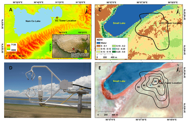
The Nam Co Station for Multi-sphere Observation and Research (NAMORS) is located about 220 km north of the Tibetan capital Lhasa (Fig. 1), on the southeast shore of the Nam Co Lake (30°46^′ N, 90°57^′ E, 4730 m a.s.l.). Strong seasonality with long, cold winters and short but moist summers is the characteristic climate prevailing in the Nam Co region (Köppen–Geiger: ET, Tundra). The mean daily temperature ranged between −22 to 14 °C during the period 2006 to 2017 (Nieberding et al., 2020b). The mean annual temperature observed according to the data from 2006 to 2017 was mostly below zero and ranged from −1.6 to 0 °C. The monthly mean temperature remained above zero in May, June, July, August, and September in all the years. The majority of the precipitation was observed from May to October (Anslan et al., 2020) with peaks either in August, July, or September. The mean annual precipitation is 405.6 mm, with the minimum and maximum precipitation ranging from 291.1 mm (2015) and 568.8 mm (2010), respectively. The soil in the regions is typical alpine steppe soil with very low clay content (Zhu et al., 2015), sustaining a mixed steppe vegetation with C₃ species like Stipa purpurea and Kobresia pygmaea with a very low plant height of 1 to 10 cm. The growing season mostly starts at the end of April or the beginning of May and extends till September, with maximum biomass in late July or August. The annual mean surface soil temperature in the study area was found to be around 9.0 °C, with mean daily values ranging from −20.1 to 34.8 °C. Surface soil moisture remained low throughout 2006–2017, with maximum value reaching up to 29 %.

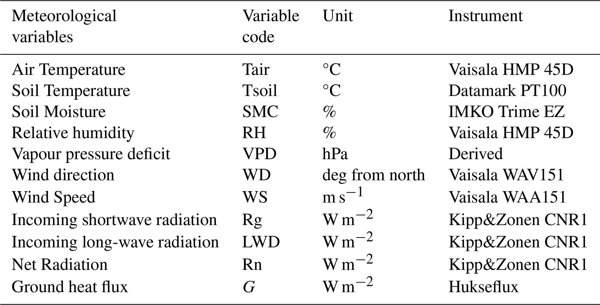
The micro-meteorological station at NAMORS consists of a 52 m tall planetary boundary layer (PBL) tower. The station is equipped with instruments (Table 1) measuring air temperature (Tair) and relative humidity (RH) at five different levels (1.5, 2, 4, 10, 20 m), wind speed and wind direction at three different levels (1.5, 10, 20 m), soil moisture (SMC) and soil temperature (Tsoil) at six different depths (0, 10, 20, 40, 80, 160 cm), soil heat flux at two different depths (10, 20 cm), radiation (short and long wave at 1.5 m), air pressure, precipitation (PPTN), and a photosynthetic photon flux density sensor (PPFD- from 2013). For detailed information on instruments, see Ma et al. (2009).

Table 1 Meteorological variables measured at site Nam Co.

The first long-term (2005–2019) eddy covariance dataset of carbon and water fluxes from the same site, measured at 3 m height (3 m EC), has been published by Nieberding et al. (2020a, b). In this study, to evaluate the fluxes at a larger spatial scale (landscape scale), a measurement unit with a CSAT3 ultrasonic anemometer and Li-7500RS open-path infrared gas analyser was installed on the PBL tower at 19 m a.g,l. (19 m EC) from July 2018 onwards (Pillai et al., 2026). The source area of the 19 m EC measurement covers a substantially broader area than that of the previously published 3 m EC dataset, encompassing alpine steppe with subtle vegetation density variations, more productive and wetter patches near the lakeshore, and occasional inclusion of the adjacent lake surface. These spatial differences in vegetation and surface cover within the 19 m footprint are integral for understanding how heterogeneity in the footprint composition influences the overall carbon dynamics within the alpine steppe ecosystem (Chu et al., 2021; Tuovinen et al., 2019).

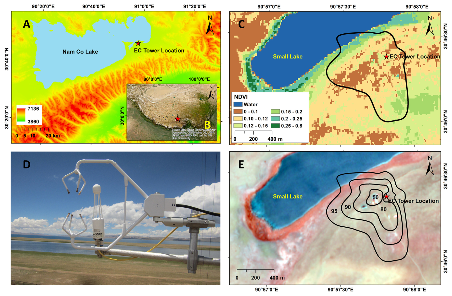
Figure 1 (A) The study area at the NAMORS station – SRTM DEM (SRTM DEM data by NASA and USGS, public domain), (B) Google Earth imagery showing the location of the Nam Co station on the TP (© Google Earth), (C) the 95 % footprint climatology overlaid on the colour-coded NDVI map derived from Sentinel 2 imagery acquired on 20 May 2019, (D) the eddy covariance (EC) measurement system at Nam Co (Photo credit: Felix Nieberding) consisting of a CSAT3 ultra sonic anemometer and an LI-7500RS open path infrared gas analyzer, (E) footprint contours representing the cumulative source area over the measurement period overlaid on Sentinel 2 imagery acquired on 20 May 2019 (Colour Infrared composite of the bands 8-4-3; Sentinel-2 imagery © Copernicus, European Union, ESA).

2.2 Eddy covariance raw data processing and quality filtering

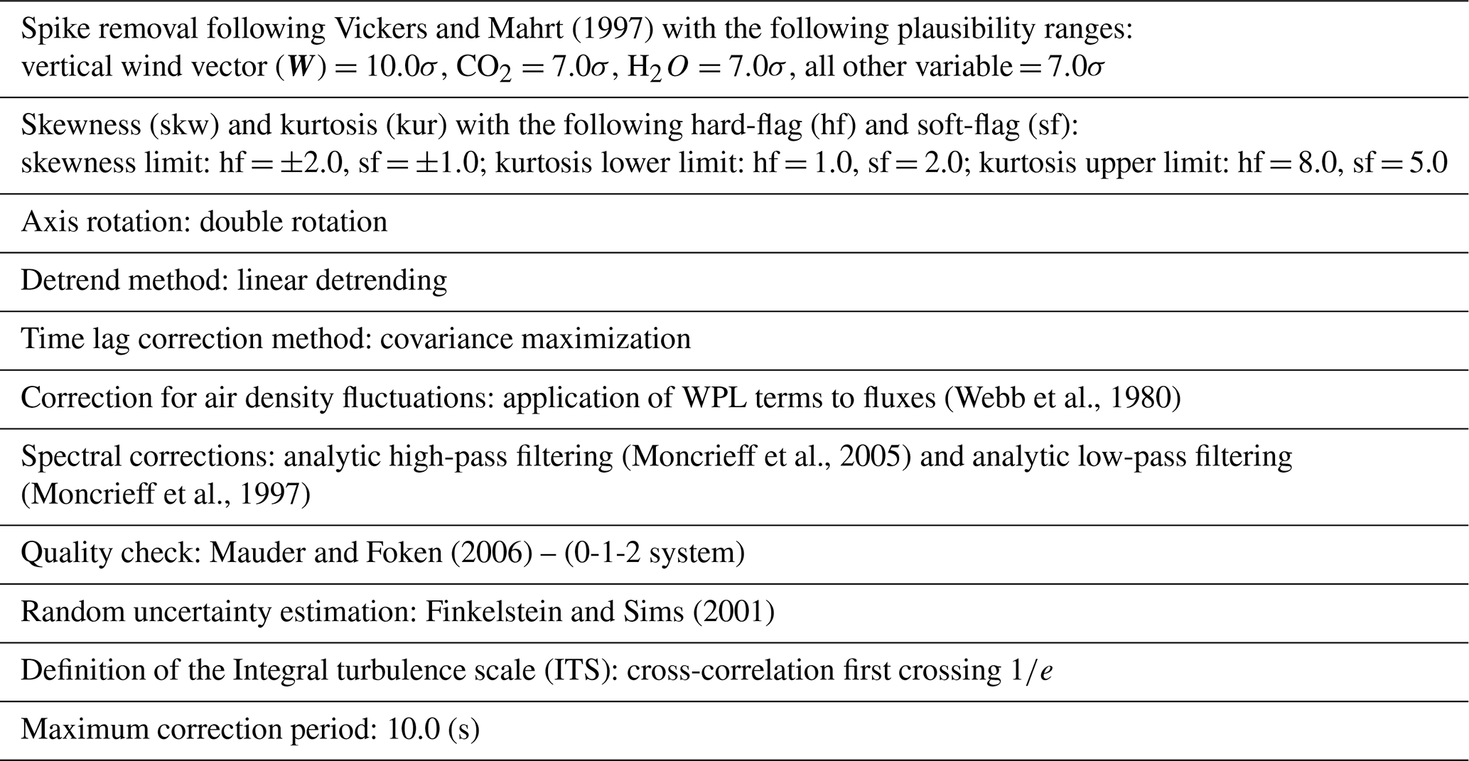
The EC method quantifies the CO₂ exchange between the surface and the overlying atmosphere by measuring the covariance between fluctuations in vertical wind velocity and CO₂ mixing ratio (Baldocchi, 2003). The 10 Hz one-year data acquired at the Nam Co site at a height of 19 m were used to calculate the 30 min averaged fluxes of CO₂ (NEE), water vapor (H₂O), sensible heat (H), and latent heat (LE) using the raw data processing software EddyPro (v7.0.9, LI-COR Inc.). The standard EC correction procedures, like despiking, coordinate rotation, detrending, data quality flagging, lag time correction, frequency response corrections/spectral corrections, SND correction, and Webb–Pearman–Leuning (WPL) corrections, were applied (Table 2).

Table 2 Flux data processing modules used in the EddyPro software (v. 7.0.9, LI-COR Inc.).

The data quality flagging policy, according to Foken et al. (2005) and Sabbatini et al. (2018), was used to remove low-quality fluxes. The combined flag attains the values 0, 1, and 2, where “0” is for best quality fluxes, “1” for fluxes suitable for general analysis, such as annual budgets, and “2” for fluxes that should be discarded from the results dataset. Only records with quality flags 0 and 1 were used for further processing and analysis, and those with quality flag 2 were retained in the data set but excluded from flux computation. In addition, NEE were excluded when both the LE and H carried a quality flag of 2, or when one of them had a flag of 2 and the other a flag of 1. This ensures that NEE is retained only when the energy fluxes used in the WPL correction are of sufficiently high quality, as low-quality H and LE measurements can propagate errors into the corrected NEE.

To remove statistical outliers, an interquartile range (IQR)-based filter was applied on a daily scale. Values outside the range defined by 1.5 times the IQR from the first and third quartiles were considered outliers. Further filtering was based on hard statistical flags exported from EddyPro. Specifically, spike detection flags (spikes_hf) and skewness and kurtosis diagnostic flags from both the low-frequency (skewness_kurtosis_sf) and high-frequency (skewness_kurtosis_hf) domains were used. These flags were parsed to extract quality indicators for CO₂, H₂O, and temperature signals. Only observations passing all relevant statistical checks (i.e., flagged as 0) were retained for each flux component. This multi-stage filtering process ensured that only physically plausible and statistically robust flux data were used in subsequent analyses.

As an additional quality control step, physiologically implausible night-time NEE values were removed. Night-time was defined as periods with incoming shortwave radiation (Rg) equal to zero, during which photosynthetic CO₂ uptake is not expected. NEE values less than zero under these conditions, indicating apparent night-time net CO₂ uptake were considered non-physical and set to missing. This step was implemented to avoid introducing artifacts into the subsequent friction velocity (u^*) threshold estimation and flux gap-filling procedures.

Periods with insufficient turbulent mixing were excluded based on the u* threshold estimated using the bootstrapped seasonal approach implemented in the REddyProc R package (Papale et al., 2006; Wutzler et al., 2018). This procedure partitions the data into seasons and applies bootstrapping within each season to derive a distribution of u^* thresholds. Thresholds were calculated for each season, based on 100 bootstrap samples. Three uncertainty scenarios (U05, U50, U95) corresponding to the 5th, 50th, and 95th percentiles of the u^* distribution were extracted. The thresholds ranged from 0.09 m s⁻¹ (U05) to 0.36 m s⁻¹ (U95) across seasons, with the U50 values varying between 0.21 and 0.27 m s⁻¹. All three u^* scenarios were retained and applied throughout the flux processing workflow (gap-filling and partitioning), allowing us to quantify uncertainty in annual and seasonal estimates of ecosystem fluxes due to u^* filtering.

2.3 Biometeorological data

The meteorological variables used for gap-filling the eddy covariance-derived fluxes include Rg, Tair, vapour pressure deficit (VPD), u^*, Tsoil, RH, and SMC. Several of these key meteorological variables, particularly Tsoil, SMC, Rg, RH, and VPD, contained long gaps during the winter months. To ensure continuity in the meteorological variables, short gaps were first filled using the Marginal Distribution Sampling (MDS) method (Falge et al., 2001; Reichstein et al., 2005), while longer gaps were filled using downscaled ERA5 reanalysis data tailored to the site level. Hourly data for soil temperature, soil water content, radiation, and RH at 9 km grid scale were obtained from the ECMWF 5th generation (ERA5) reanalysis data (C3S, 2018; Copernicus Climate Change Service, 2019) and were linearly interpolated to half-hourly intervals to match the temporal resolution of EC flux measurements. These interpolated datasets were then downscaled to the site level using in situ meteorological observations. Downscaling was achieved by developing empirical models based on overlapping periods between ERA5 and observed site-level data. Linear regression models were used for most variables. However, for cases where linear models failed to capture nonlinear relationships, random forest (RF) models were applied.

2.4 Gap filling and flux partitioning

Marginal distribution sampling (MDS) algorithm (Falge et al., 2001; Reichstein et al., 2005) and RF (Breiman, 2001; Stekhoven and Bühlmann, 2012) were used for gap filling. To evaluate the accuracy of each method, we performed a cross-validation approach by artificially masking 20 % of the valid data for each flux variable (NEE, LE, and H). We repeated this procedure 10 times with different random seeds. Model predictions were then compared to the withheld true values using statistical metrics including root mean square error (RMSE) and its standard deviation (SD).

2.4.1 Marginal distribution sampling (MDS)

The data gaps in the flux measurements after all quality controls were filled using the REddyProc R package (Wutzler et al., 2018) to apply the MDS gap-filling algorithms. This approach fills gaps by identifying periods with similar meteorological conditions and temporal proximity, using both the fluxes and driving environmental variables, thereby accounting for temporal autocorrelation and conditional similarity (Reichstein et al., 2005). The half-hourly NEE values were partitioned into gross primary productivity (GPP) and ecosystem respiration (Reco) using the day time based method of Lasslop et al. (2010), which uses the common rectangular hyperbolic light-response curve (Falge et al., 2001) to model NEE. The method accounts for the temperature sensitivity of Reco and includes VPD limitation on GPP.

2.4.2 Random Forest (RF)

High-altitude EC sites often experience substantial data gaps following quality control filtering, due to harsh environmental conditions and limitations in instrument maintenance. Although MDS is widely used as a standard method for gap-filling in many flux networks, especially for short to medium gaps, its accuracy may decline in the presence of longer or more frequent gaps. In such cases, machine learning approaches like RF can offer improved performance by capturing complex, nonlinear relationships between environmental drivers and fluxes (Irvin et al., 2021; Kalhori et al., 2024). Although originally developed for modelling tabular data, RF has recently been applied to gap-filling flux data in EC research (Wang et al., 2025b; Zhang et al., 2023). In this study, RF-based gap filling was implemented using the missForest package in R (Stekhoven and Bühlmann, 2012). The same predictor variables used in the MDS method were applied, allowing for a direct comparison of their performance under similar conditions.

2.5 Uncertainty estimation

EC flux measurements are subject to uncertainties arising from various sources. These include both systematic uncertainty, due to limited sensor maintenance, and random uncertainty, which arises from the stochastic nature of turbulence and footprint variability (Loescher et al., 2006). To comprehensively characterize the overall uncertainty in the flux estimates, we considered multiple components like random flux error (RE), gap-filling model uncertainty (standard deviation of the gap-filled estimate), and the friction velocity (u^*) threshold uncertainty. RE associated with the measurements was calculated using the mathematically rigorous and fully implemented approach by Finkelstein and Sims (2001). Gap-filling model uncertainty comes from the model structure in the MDS gap-filling. The value reflects how confident the gap-filling is under given meteorological conditions. The u^* threshold uncertainty arises from the uncertainty in selecting the friction velocity threshold, which affects the fraction of data filtered and the subsequent gap-filling, thereby influencing the final flux estimates.

For each half-hourly record, uncertainty was assigned using RE for observed fluxes and gap-filling standard deviation for gap-filled values. These half-hourly uncertainties were then propagated to daily and monthly sums using root-sum-of-squares error propagation, assuming independence of components. The u* threshold uncertainty was reported separately as the spread of flux estimates across different threshold scenarios. This approach provides a robust characterization of both statistical (measurement and gap-filling) and methodological (u^* threshold) uncertainties in the reported carbon fluxes.

2.6 Footprint

The relative contribution from each element of the surface area source/sink to the measured vertical flux at a specific point in time, for specific atmospheric conditions and surface characteristics, is termed “flux footprint” (Kljun et al., 2015; Leclerc and Foken, 2014; Vesala et al., 2008). The measurement height, along with surface roughness and wind direction, determines the dimension of the area contributing to a given flux measurement. Above a homogenous surface and under turbulent mixing conditions, the fluxes do not vary in space and contribute equally to the flux strength; hence, the height of a sensor should not influence the measurements. However, the height of the sensor and atmospheric conditions matter on an inhomogeneous surface because the measured signal at the sensor depends on the part of the surface that has the strongest influence (Schmid, 2002).

The major approaches used in footprint modelling include analytical models, Lagrangian stochastic particle dispersion model (LPDM), large eddy simulations (LES), and closure models (Vesala et al., 2008). The current study used the Kormann and Meixner (KM) footprint model (more details in Kormann and Meixner, 2001) to analyze the influence of the source area on the measured fluxes. The KM model is based on a modification of the analytical solution of the advection-diffusion equation for power law profiles of the mean wind velocity and eddy diffusivity. The model uses parameters like EC measurement height (zm) in meter (m), roughness length (z0) in m, mean wind speed (WS) in m s⁻¹, Monin–Obukhov length (L) in m, the standard deviation of crosswinds (sv) in m s⁻¹, friction velocity (ustar) in m s⁻¹, and wind direction (WD) in degrees (Table S1 in the Supplement). All variables were obtained from the processed EC data in EddyPro, except for z0, which was dynamically calculated for each half-hourly period using the Kormann and Meixner (2001) approach based on the measured ustar, WS, WD, L, and zm with quality control flags applied to filter invalid values.

Half-hourly KM footprint probability matrices were generated and overlaid with the land cover map (Fig. S2). The land cover map was created by visual interpretation of cloud-free Sentinel-2 Level-1C (L1C) MSI imagery acquired for the site. The data were downloaded for cloud-free dates from Google Earth Engine. All bands were downloaded separately and stacked into multi-band images across multiple dates to facilitate visual comparison during digitisation. The base image used for digitisation was acquired on 20 May 2019. Each stacked image had a spatial resolution of 10 m. Digitization of land cover units was performed on a colour infrared RGB composite using bands 8 (Near Infrared; 833 nm), 4 (Red; 665 nm), and 3 (Green; 560 nm). For each half-hourly period, the footprint probability of each pixel was multiplied by a binary mask of each land cover class (1 if the pixel belongs to that class, 0 otherwise), and the weighted values were summed over all pixels to calculate the fractional contribution of each class to the total footprint area.

2.7 Energy balance closure

Energy balance closure (EBC) was calculated using the turbulent fluxes (H+LE) and the available (Rn−G) energy using the 30 min measurements. Observations from the growing season were used for the calculation. Net radiation (Rn) was calculated from the incoming and outgoing shortwave and long-wave radiation. The incoming long-wave radiation (LWD) was unavailable due to sensor failure for the entire published dataset period. In order to provide an estimate of the energy balance closure during this period, we estimated LWD following the approach of Brutsaert (1975), using Tair, RH, and cloud cover fraction (estimated using Rg). The method was tested and calibrated using the period during which LWD at the site was available (2006–2017). The ground heat flux (G) measurements were shifted forward by 30 min, taking the soil measurement lag into consideration (Li et al., 2015).

For the published dataset period, the EBC at the study site showed 75 % closure. This is consistent with previously and recently published results from the Nam Co region: Biermann et al. (2014): 70 %, Li et al. (2015): 78 %, and Wang et al. (2026): 82.8 %. The small variations between these values could be likely due to the different measurement footprints in the complex heterogeneous terrain at Nam Co. These values fall within the energy balance closure range (60 % to 90 %) reported for EC systems in complex and heterogeneous terrain (Foken, 2008; Foken et al., 2011; Twine et al., 2000; Yao et al., 2011).

3 Results

3.1 Data and quality filtering

The data described in this article extend from 14 July 2018 to 8 June 2019, with all times reported in China Standard Time (CST, UTC+8). Raw data coverage was high (91 %–93 % for NEE, LE, and H), but decreased progressively with each QA/QC step. The fractions of best quality data retained after all quality filtering were 32.8 %, 43.8 %, and 35.1 % for NEE, LE, and H, respectively. Figure 2 illustrates the data availability of NEE and energy fluxes, and Table S2 summarizes the percentage of data retained after each filtering stage, providing a transparent record of dataset quality and reuse potential.

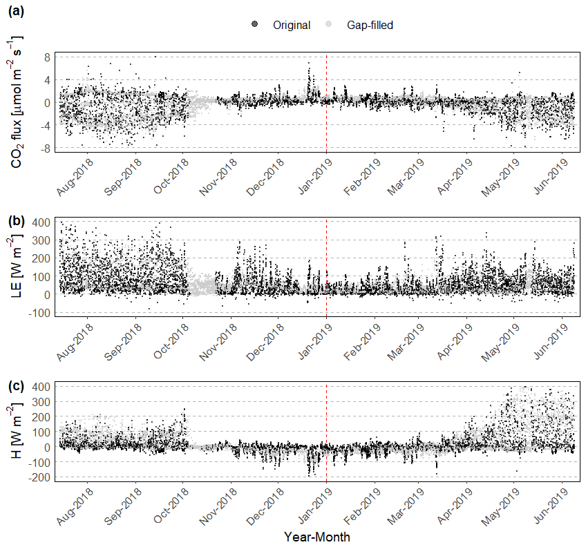
Figure 2 Time series of half-hourly fluxes from July 2018 to June 2019. (a) Net ecosystem exchange (NEE), (b) latent heat flux (LE), and (c) sensible heat flux (H). For each flux, the black points represent the original measured values, while the grey points indicate gap-filled fluxes using marginal distribution sampling (MDS). The dashed red vertical lines indicate the start of 2019. Units are µmol m⁻² s⁻¹ for NEE and W m⁻² for LE and H. To enhance visual clarity, the y axis was truncated. The values outside the displayed range are omitted from the figure but remain included in the dataset and analysis.

The dataset also includes site-measured meteorological variables, meteorology from ERA5 reanalysis data, and the ERA5 meteorology data downscaled to the site level. The temporal coverage of site-measured variables, mainly soil parameters (Tsoil, SMC), RH, VPD, and Rg was approximately 50 % or higher, with longer gaps during winter months. To provide continuous coverage, these measurements are complemented by downscaled ERA5 estimates at the site level. The downscaled estimates showed a strong agreement with observed site-level measurements, with R² values exceeding 0.93. The RMSEs of the downscaled Tsoil, SMC, Rg, RH, and VPD were 0.58 °C, 0.002 %, 116 W m⁻², 3.41 %, and 0.65 hPa, respectively (Fig. S1 in the Supplement, Table S3). These results indicate that the gap-filled meteorological data reliably capture site-level conditions.

3.2 Gap filling

Among the two gap-filling methods (MDS & RF) evaluated, RF consistently outperformed MDS across all flux variables (NEE, LE, and H). The accuracy of the gap-filling methods was summarized in Table S4. For NEE, the mean RMSE decreased from 0.66±0.04 µmol m⁻² s⁻¹ with MDS to 0.52±0.06 µmol m⁻² s⁻¹ with RF. For energy fluxes, the mean RMSE declined from 29.13±0.67 W m⁻² to 4.42±0.59 W m⁻² for LE, and from 18.55±0.74 W m⁻² to 10.54±0.46 W m⁻² for H. Both MDS-based and RF-based gap-filled values are included in the dataset, with quality flags indicating whether values are observed or gap-filled.

3.3 Source area contribution

The overall footprint contributions during the study period, based on the half-hourly data, indicated that the main steppe (MSteppe) was the dominant source area, accounting for 69.4±22.3 % (mean ± SD) of the flux footprint. Lake surfaces, vegetation on the lake shore, and the vegetation on SW contributed 14.4±16.6 %, 6.9±5.8 %, and 6.2±6.0 % respectively (Table 3). The spatial distribution of each land cover class used in the footprint analysis is shown in Fig. S2. The wind-sector weighted footprint contributions (Fig. 3) illustrate how the relative importance of each land cover class varies with wind direction. The relatively large standard deviations reflect high temporal variability in source area contributions, driven by changes in wind direction and atmospheric stability. Footprint distances indicate that the median contribution (d50) originated from 351 m, with 80 % of the flux (d80) captured within 784 m and 90 % (d90) within 1.28 km of the tower, demonstrating the landscape-scale representativeness of the measurements.

Table 3 Overall contributions of land cover classes to the eddy covariance flux footprint at the 19 m tower. Values are reported as mean ± standard deviation (SD, %), based on filtered data with best quality flag (qc_flag = 0). MSteppe = Main Steppe; SW = Southwest. The corresponding wind-sector polar plot (Fig. 3) illustrates how these contributions vary with wind direction.

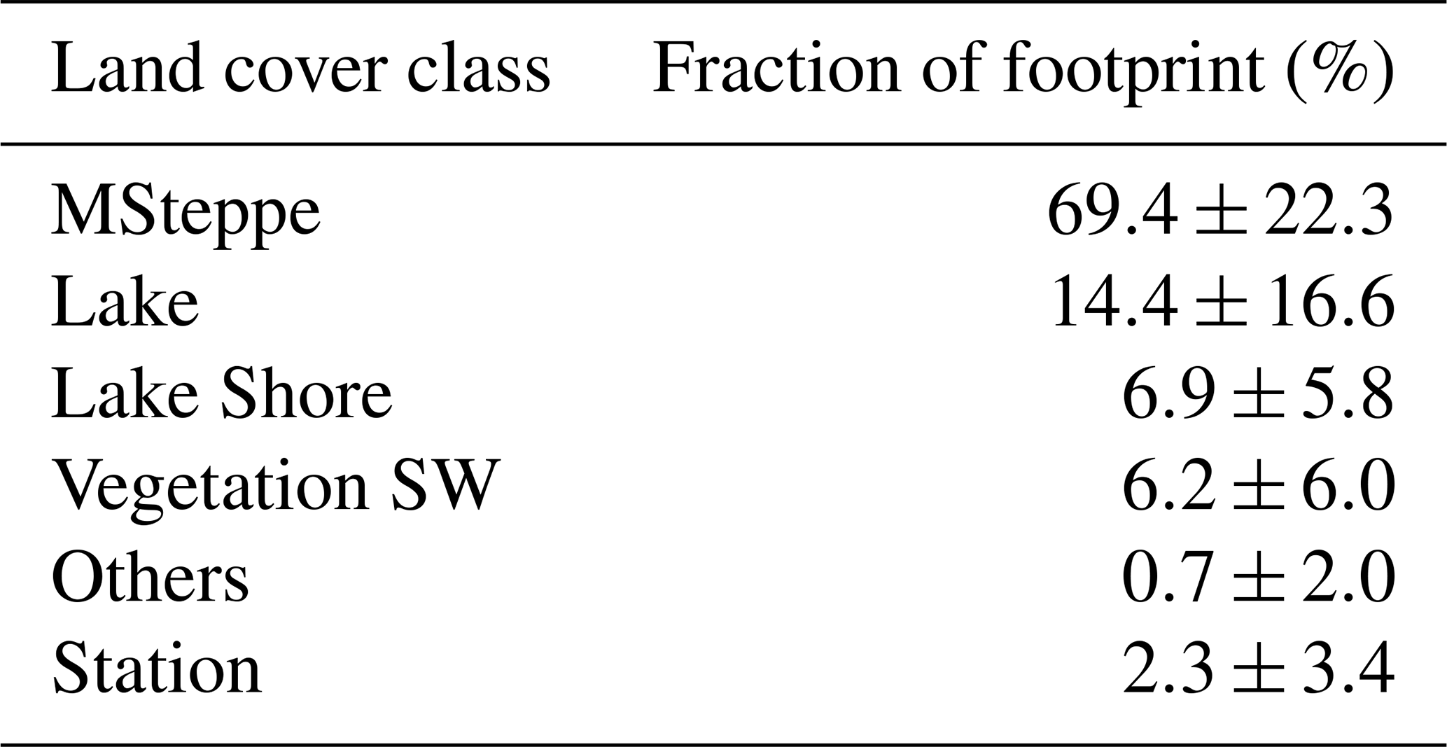
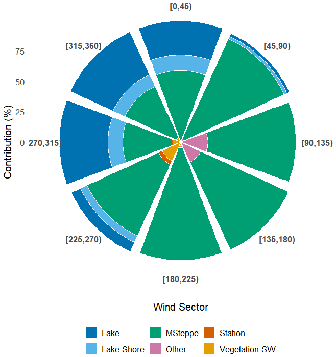
Figure 3 Wind-sector weighted footprint contributions of land cover classes to the eddy covariance fluxes at the 19 m tower. Each sector represents an 8-point compass division of wind directions. The radial length shows the percentage contribution of each land cover class to the flux footprint, and stacked colours indicate the relative percentage contribution of different land cover classes within each wind sector. Data were filtered for qc_flag = 0.

3.4 Flux uncertainty estimation

Half-hourly NEE uncertainties, combining RE and gap-filling uncertainty (NEE_U50_fsd), exhibited clear diurnal and seasonal patterns (Fig. 4a). The RE remained lower than the NEE_U50_fsd with medians of 0.43 and 0.67 µmol m⁻² s⁻¹, respectively. A similar pattern was observed for LE (RE = 7.10 and LE_U50_fsd = 28.61 W m⁻²) and H (RE = 3.86 and H_U50_fsd = 23.90 W m⁻²).

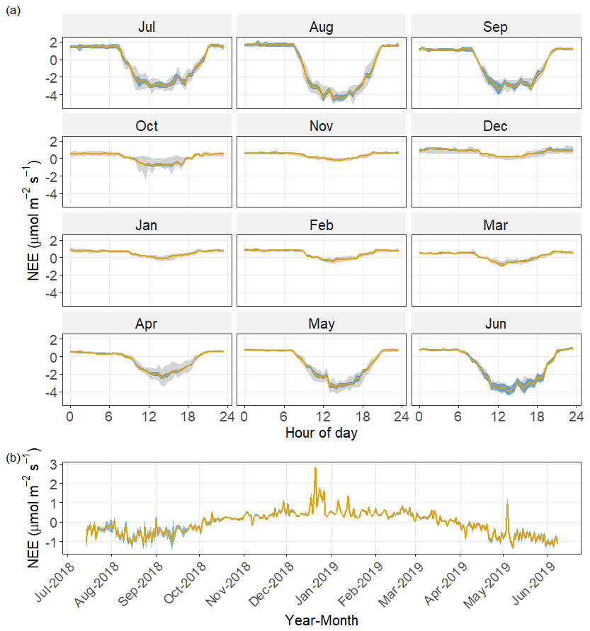
Figure 4 (a) Diurnal cycle of net ecosystem exchange (NEE) for each month from July 2018 to June 2019. The orange line represents the mean gap-filled NEE (U50). Blue shaded ribbons indicate ±1σ combined uncertainty, including both random measurement error and gap-filling uncertainty. Grey shaded ribbons show the interquartile range (25th–75th percentile) of half-hourly NEE values, reflecting day-to-day variability; (b) daily mean net ecosystem exchange (NEE) from July 2018 to June 2019. The orange line represents the daily mean gap-filled flux (U50). Blue shaded ribbons indicate the propagated daily uncertainty, combining random measurement error and gap-filling uncertainty.

During the growing months (May, June, July, August, and September), mid-daytime (10–14 h) uncertainties averaged 1.34 µmol m⁻² s⁻¹, compared to 0.43 µmol m⁻² s⁻¹ in winter (October - April). Nighttime (Rg < 5) uncertainties were lower overall and showed smaller seasonal differences (GS mean 0.66 vs. winter mean 0.43 µmol m⁻² s⁻¹). These results indicate that measurement and gap-filling uncertainties are generally higher during periods of high flux activity (daytime in the growing season) and lower at night and in winter. A full set of descriptive statistics is provided in Table S5.

Daily uncertainties, propagated from half-hourly values using root-sum-of-squares, were smaller than half-hourly values, with a mean of 0.11 µmol m⁻² s⁻¹, a median of 0.09 µmol m⁻² s⁻¹, and a maximum of 0.63 µmol m⁻² s⁻¹ (Fig. 4b). The interquartile range of half-hourly NEE (grey ribbons in Fig. 4a) was consistently larger than the statistical uncertainty, particularly during the growing season, highlighting the contribution of natural variability to overall flux dynamics.

Similar diurnal and seasonal patterns of uncertainty were observed for LE and H (Figs. S3 and S4), with higher uncertainties during the growing season and generally lower values in the non-growing season. During the growing season, daytime uncertainties exceeded nighttime values, whereas in the non-growing season, nighttime uncertainties were comparable to or slightly higher than daytime values.

Methodological uncertainty associated with the u^* threshold exhibited distinct seasonal behaviour (Fig. 5). For NEE and H, u^* threshold-related uncertainty was highest during winter. In contrast, for LE, u^* threshold-related uncertainty was present throughout the year but increased during periods of active surface–atmosphere exchange. Overall, statistical uncertainty dominated during periods of active fluxes, whereas methodological uncertainty could exceed statistical uncertainty for NEE and H in winter.

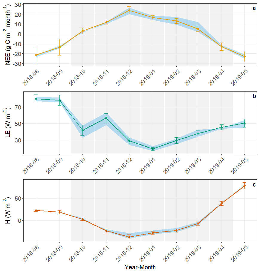
Figure 5 Monthly aggregated fluxes at the Nam Co site from August 2018 to May 2019: (a) net ecosystem exchange of CO₂ (NEE, g C m⁻² per month), (b) latent heat flux (LE, W m⁻²), and (c) sensible heat flux (H, W m⁻²). Shaded blue ribbons indicate the spread between the 5 % and 95 % u^* filtering scenarios. Orange (NEE), green (LE), and red (H) lines and points represent the median estimate (50 % scenario). Vertical error bars denote the total monthly uncertainty, including random error and gap-filling uncertainty. Grey background shading highlights the non-growing season (NGS, October–April), while unshaded periods represent the growing season (GS, May–September). Partial months (July 2018 and June 2019) were omitted to avoid bias.

4 Discussion

4.1 Data quality, gap-filling and uncertainty

The dataset presented here provides a continuous record of carbon and energy fluxes from an alpine steppe environment on the Tibetan Plateau, measured at 19 m a.g.l. to capture landscape-scale processes. Overall, the data exhibit high quality and completeness, despite the harsh climate and logistical constraints typical of high-altitude regions. The raw data coverage exceeded 90 % across all fluxes, but subsequent filtering and quality control reduced the proportion of high-quality fluxes to around one-third to one-half of the total, which is in line with the reductions typically reported for alpine eddy covariance datasets (Hiller et al., 2008; Nieberding et al., 2020a). While this reduction highlights the challenges of ensuring reliable measurements in complex environments, the provision of detailed quality flags alongside each flux value allows users to tailor data usage according to their specific needs.

Among the two widely adopted gap-filling methods, RF consistently outperformed MDS across all flux variables, reducing root mean square errors by 20 %–80 % depending on the flux. This improvement likely reflects the ability of RF to capture non-linear relationships between fluxes and their drivers when the gaps are large (Irvin et al., 2021). Although RF produced more accurate gap-filled values in this case, MDS remains a valuable method, especially due to its wide adoption in FLUXNET and other synthesis efforts. By including both MDS and RF-based gap-filled values in the dataset, we allow users to choose the approach most appropriate for their intended analyses.

Uncertainty analyses revealed distinct seasonal and diurnal patterns, with higher uncertainties during the growing season and daytime, when fluxes are largest and most variable (Richardson et al., 2006). Statistical uncertainties from random error and gap-filling were generally dominant, but methodological uncertainty related to the u^* threshold became more important during winter for NEE and H, and during periods of active surface–atmosphere exchange for LE. While daily aggregations substantially reduced uncertainty, caution is necessary when interpreting short-term flux variability. The inclusion of multiple uncertainty estimates in this dataset enhances its value for model benchmarking and data–model integration, providing users with the flexibility to account for different error sources.

4.2 Footprint analysis and implications

The footprint analysis ensures that the dataset is representative of the target ecosystem type, the “alpine main steppe”. At the same time, contributions from adjacent surfaces, including lake water, shoreline vegetation, and mixed southwest vegetation, accounted for approximately 25 %–30 % of the footprint. These secondary sources may influence certain flux components, particularly latent heat fluxes, due to differences in surface energy balance between steppe and aquatic environments. The NW sector remained inherently mixed (MSteppe, Lake, Lake Shore), with a considerable contribution from lake (14.4±16.6 %, mean ± SD over the study period). For half-hours when the footprint is dominated by mixed contributions (e.g., the NW sector), the flux signal cannot be decomposed into surface-type-specific components without introducing additional assumptions. However, the footprint contribution diagnostics included in the dataset allow users to identify and select time periods where the footprint is dominated by a single class such as MSteppe, enabling flux estimates that are effectively representative of that surface type alone. In contrast, lake and lake shore are almost never the dominant contributor to the footprint on their own, so flux estimates specific to these surfaces cannot be reliably isolated from this dataset. We note that this filtering approach is optional and intended for users seeking surface-specific flux estimates. Since footprint-dominant periods are linked to wind direction, removing non MSteppe timestamps creates gaps that are not random but clustered by wind sector. Gap-filling such clustered, extended gaps is more uncertain than gap-filling the short, scattered gaps in the original dataset. Users should account for this added uncertainty when calculating cumulative or aggregated fluxes from a filtered subset.

The footprint distances (median ∼350 m, 80 % within ∼780 m, 90 % within ∼1200 m) are consistent with landscape-scale representativeness and align with expectations for low-roughness open steppe environments. The spatial scale of the measurements integrates a greater degree of land cover heterogeneity compared to the 3 m EC system previously operated at this site (Nieberding et al., 2020a), whose smaller, more homogeneous footprint primarily sampled the main steppe area alone. Unlike the typical EC system on grasslands, which represents a smaller footprint area, the larger footprint achieved by the current measurement setup allows for a more representative comparison and validation with satellite GPP products such as Moderate Resolution Imaging Spectroradiometer (MODIS). The area encompassing 90 % of the footprint climatology over the study period corresponds to a source area of approximately 280 000 m², closely matching the area of a single MODIS pixel (∼250 000 m²), making the dataset a valuable resource for potential data users. Spatial representativeness may vary under wind directions or stability conditions. The inclusion of footprint diagnostics and the input variables needed to derive footprints in the dataset allows users to evaluate this variability directly for their specific applications. The larger footprint, together with the auxiliary meteorological variables provided in this dataset, further supports its use in land surface and ecosystem models requiring landscape-scale representation of vegetation, soil moisture, and temperature heterogeneity.

Taken together, the dataset provides a transparent and high-quality record of ecosystem–atmosphere exchanges in a sparsely monitored region. Its strengths include high raw data coverage, the application of two complementary gap-filling approaches, detailed footprint characterization, and a thorough assessment of uncertainties. These elements ensure that the dataset provides a reliable reference for short-term analyses of carbon and energy dynamics in high-elevation grassland systems on the TP and forms a valuable foundation for future long-term monitoring efforts.

Scale mismatch continues to be one of the major issues in model-data integration and satellite validation. The magnitude and sign of biases associated with relating individual tower footprints to the spatial extent of model or satellite data products vary considerably across sites, with fixed-extent approaches introducing errors of 4 %–20 % for EVI and 6 %–20 % for dominant land-cover (Chu et al., 2021). By capturing a larger footprint through 19 m measurement height at this site, the dataset reduces spatial mismatch between the flux footprint and commonly used satellite products such as MODIS, providing flux observations that are more comparable to the MODIS grid cell (10⁵–10⁶ m²). This improves their suitability for satellite-product evaluation, model benchmarking, and upscaling studies.

5 Code and data availability

The data set and the R scripts were uploaded to GFZ Data Services and will be freely available at https://doi.org/10.5880/GFZ.TKVR.2026.001 (Pillai et al., 2026). The data sets are published under a Creative Commons Attribution 4.0 International (CC BY 4.0) license.

6 Conclusion

Here, we present a continuous record of carbon and energy fluxes measured at a landscape scale in an alpine steppe ecosystem on the Tibetan Plateau, covering the period from July 2018 to June 2019. Despite the challenges of eddy covariance measurements in this harsh environment, rigorous quality control ensured the reliability of the dataset. Alongside fluxes with accompanying quality flags, the dataset includes results from dual gap-filling approaches, detailed half-hourly footprint characterization, auxiliary meteorological measurements, and comprehensive uncertainty estimates, providing transparency and usability for diverse applications. Data are provided at three temporal resolutions (half-hourly, daily, and monthly) for fluxes, along with separate datasets for site meteorology and ERA5 reanalysis data. By integrating across the heterogeneous alpine steppe landscape, this dataset fills a critical observational gap in one of the world's most climate-sensitive regions and provides a robust foundation for ecosystem process studies, model evaluation, and satellite product validation.