The multi-temporal landslide inventory map of the Collazzone study area, central Italy

Multi-temporal landslide inventory maps are an essential source of information for many research and applications. This type of landslide map provides information for analyzing the spatial and temporal distribution of the landslides, their potential interaction with the structure and infrastructure, their contribution to landscape dynamics, and their response to the triggers over time. The acquisition of the temporal information of landslide evolution provides a fundamental step for hazard evaluation. Despite the essential value of multi-temporal landslide inventory maps, their dissemination is rare. This is due to the time-consuming nature of their preparation. In this paper we present the multi-temporal landslide inventory map for a 79 km² area, Collazzone study area, in the Umbria region (central Italy). The inventory contains more than 3500 landslides classified according to relative age, type of movement, and estimated depth. The landslide mapping was carried out by interpreting stereoscopic aerial photographs taken in 1941, 1954, 1977, 1985, and 1997, as well as stereo satellite images taken in 2010, 2013, and 2014. The inventory was further updated through several field checks conducted in 1999, 2004, 2005, and 2020, and by interpreting the images available on Google Earth (2011, 2012, 2015, 2015, 2015, 2019, 2021, 2022 and 2023). Landslides were mapped according to rigorous and reproducible criteria applied by a team of expert geomorphologists. The dataset consists of a digital archive including twenty-nine layers, that is available at https://doi.org/10.5281/zenodo.21531647 (Ardizzone, 2026).

1 Introduction

A landslide inventory map (LIM) records the location and, where known, the date of occurrence and the types of mass movements that have left discernible traces in an area (Guzzetti et al., 2000; Pašek, 1975). Landslide inventory maps are crucial for the following purposes (Guzzetti et al., 2012): (i) recording the extent of landslide phenomena in a certain area; (ii) evaluating landslide susceptibility, hazard, and risk; (iii) investigating the distribution, type and patterns of landslides; and (iv) studying the evolution of landscapes. Among the different types of LIMs (Ardizzone et al., 2023; Guzzetti et al., 2012) the multi-temporal landslide inventory map (M-LIM) shows the location and types of landslides triggered by multiple events over longer periods (e.g., years to decades) and portrays their recent evolution in space and time (Galli et al., 2008). A multi-temporal inventory map allows to investigate the spatial and temporal evolution of landslides in several different time periods showing areas with different frequency of landslide occurrence (Zumpano et al., 2021). Moreover, the temporal dimension of a multi-temporal landslide inventory map is essential for the evaluation of the landslide hazard.

Galli et al. (2008) showed that an inventory prepared through the systematic and simultaneous interpretation of several sets of stereo aerial photographs of different age, supplemented by extensive geological and geomorphological field surveys, is superior to (i.e., more reliable than) geomorphological or reconnaissance inventories prepared for the same study area. However, due to the time required to complete an inventory, such a type of map cannot be effectively prepared for a large region, extending for thousands of square kilometers. Consequently, multi-temporal landslide inventory maps have been prepared for areas of limited size (Cardinali et al., 2002; Zumpano et al., 2021). Examples of multi-temporal landslide inventory maps prepared for large area were presented in 2005 (Guzzetti et al., 2005) for a 275 km² study area located in in the southern Lombardy region (northern Italy), in 2006 (Guzzetti et al., 2006b) for a 79 km² study area in central Italy and in 2007 (Cardinali et al., 2007) for a 590 km² study area in the central Abruzzo region (central Italy). These landslide maps were prepared by interpreting different sets of stereo aerial photographs (from 2–5 sets) taken in the period from 1941 through 1997, and field surveys.

Traditionally, landslide inventories have been compiled through the interpretation of multiple sets of aerial photographs. However, recent studies have increasingly integrated additional data sources. Del Ventisette et al. (2014) presented the results obtained, in two study areas in northern Italy, by the interpretation of A-DInSAR satellite dataset, spanning from 1995 through 2009 and their integration with geological and geomorphological data to obtain an updating of landslide inventory map. Recently, Fernández et al. (2021) used aerial photogrammetry and LiDAR techniques to analyze landslide activity over a long-time span (over 32 years), from 1984–2001 in a 51 km² study area in Spain.

Amatya et al. (2024) used high-resolution satellite imagery to generate a multi-temporal landslide inventory for the Arun River Basin, Nepal. The inventory represents a yearly record of landslides from 2011 through 2020. Li et al. (2024) proposed an innovative unsupervised learning method (called PluTsa) for multiple temporal landslide inventory mapping in Japan by using Planet Scope imagery acquired in May 2019, in October 2020, in August 2021 and in October 2022.

Information on landslide locations, types, and sizes, combined with data on temporal occurrence, is crucial to evaluate the hazard posed by landslides. Nevertheless, multi-temporal landslide maps are rare and their recent increase is due to the availability of remote sensing technology and the use of artificial intelligence models (Bhuyan et al., 2023a). Bhuyan et al. (2023b) used Deep Transfer Learning approach applied to High Resolution Planet Lab images, spanning from 2009 through 2021, to generate annual landslide inventories in view of the preparation of a multi-temporal landslide inventory map.

In this paper we present the multi-temporal landslide inventory map prepared for the Collazzone study area, in Umbria region, central Italy, an area historically affected by shallow and deep landslides. The landslide inventory map was produced using multiple data sources. The inventory was prepared through the interpretation of five sets of stereoscopic aerial photographs, taken in 1941, 1954, 1977, 1985, 1997, of stereo satellite images taken in 2010, 2013 and 2014. The inventory was updated through several field checks conducted in 1999–2000, 2004, 2005, 2020 and through the interpretation of the images available on Google Earth: 2011-04-02, 2012-05-10, 2015-03-14, 2015-07-08, 2018-04-08, 2019-10-08, 2021-04-28, 2022-03-23, 2023-05-30. The multi-temporal landslide inventory map of Collazzone (M-LIM-C) represents the product of a work that began in the early 2000s. The M-LIM-C was used to perform several studies such as evaluation of hazard and risk (Guzzetti et al., 2006b, a, 2009a; Lombardo et al., 2020; Mergili et al., 2014; Rossi et al., 2010); sediment mobilization rate (Fiorucci et al., 2011; Guzzetti et al., 2009b); understanding the “legacy effects” of the landslides (Samia et al., 2017a, b, 2018, 2020).

2 Study area

The Collazzone area, located in central Umbria (Italy), extends for about 79 km² with elevations ranging from 145 m along the Tiber River floodplain to 634 m at Monte di Grutti (Fig. 1A). The landscape is predominantly hilly, and the lithology and the attitude of bedding planes control the morphology of the slopes. North–south valleys are shorter, asymmetrical, and parallel to the main direction of the bedding plains, whereas east–west valleys are longer, symmetrical, and mostly perpendicular to the direction of the bedding planes. Sedimentary rocks crop out in the area including (Fig. 1B): (i) alluvial deposits, chiefly along the main valley bottoms, (ii) Plio-Pleistocene continental gravel, sand and clay, (iii) Pleistocene travertine deposits, (iv) Miocene layered sandstone and marl in various percentages, and (v) thinly layered limestone, Lias to Oligocene in age (Conti and Girotti, 1977; Servizio Geologico Nazionale, 1980; Cencetti, 1990; Barchi et al., 1991). The terrain is hilly, valleys are asymmetrical, and slopes are controlled by lithology and the attitude of bedding. Soil in the area ranges in thickness from a few decimeters to more than one meter, they have a fine or medium texture, and exhibit a xenic moisture regime, typical of the Mediterranean climate with precipitation falling mostly in the period from October–December and from February–May. Annual average rainfall is about 740 mm (from 2000–2024) measured at the Collepepe rain gauge (Fig. 1A). The land use includes cropland, forest, vineyard and orchard, and urban areas (Fig. 1C).

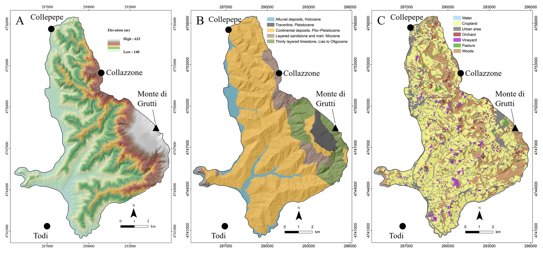
Figure 1 Collazzone study area: (A) elevation map; (B) lithological map; (C) land use map.

Landslides are abundant and are caused primarily by meteorological triggers, including prolonged rainfall and rapid snowmelt (January 1997), no historical information of earthquake-induced landslides exists for the study area (https://sici.irpi.cnr.it/, last access: 8 June 2026). Appendix B presents a histogram of the cumulative monthly rainfall and mean monthly precipitation recorded at the Todi rain gauge (location shown in Fig. 1A) for the period 1940–2023. The mean annual rainfall during this period is approximately 849 mm. The histogram also displays, as black dots, the dates corresponding to the landslide inventory layers (Table 1). Ardizzone et al. (2007, 2013) and Fiorucci et al. (2011) investigated the rainfall conditions associated with landslides triggered by precipitation events occurring after 2000, whereas examined the snowmelt event that affected the Umbria Region in 1997 and triggered numerous landslides, including several within the study area (E₂ in Table 1).

They can be classified as rapid to very slow, shallow soil slides and flows, deep-seated slides and flows, and compound movements (Galli et al., 2008; Guzzetti et al., 2006a, b).

3 Material and method

The preparation of M-LIM-C has been ongoing for nearly two decades, employing various methods for landslide mapping. The inventory is periodically updated following significant landslide events and is subject to regular field checks to validate and refine the mapped information. We employed a multi-stage approach rather than a single procedure, with activities conducted overtime (Fig. 2). The overall work consisted of three main stages: (i) data acquisition (e.g., landslide interpretation and field survey), (ii) data editing (e.g. digitalization in GIS environment), and (iii) finalizing the results (i.e., the geodatabase).

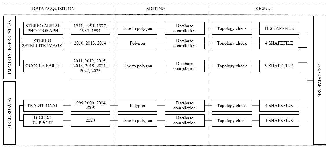
Figure 2 Schema of the work carried out to obtain the M-LIM-C. The activity includes three phases: data acquisition, editing and results. The two methods used to map the landslides are: photo interpretation and field surveys.

The M-LIM-C was prepared at a 1:10 000 scale through the interpretation of five sets of aerial photographs (Table 1) and extensive geological and geomorphological field mapping (layers A₀ to E₂ in Table 1). This initial work constituted the core of the landslide inventory map, which has been subsequently expanded and updated over time. The map was updated in the period from 1999 through 2005 through field surveys conducted following periods of prolonged rainfall to map landslides triggered by heavy rainfall (layers F₁ to F₄ in Table 1). Between 2009 and 2014, the inventory was improved by incorporating landslide maps prepared using VHR stereo satellite imagery (layers G₁, G₂, G₅ and G₆ in Table 1). In December 2020, a field survey mapped new landslides triggered by several days of intense rainfall (F₅ in Table 1). Additional landslides were identified through Google Earth at different dates (Table 1).

Table 1 List of the layers included in the M-LIM-C. ELA: estimated landslide age. P-I: photo interpretation. F-S: field survey. GSD: ground sample distance. The letters from A–E indicate the layer prepared by the photointerpretation of the stereo-aerial photographs. The letter F indicates the layers prepared through field surveys. The letter G indicates the layers prepared using satellite imagery. NA means not applicable.

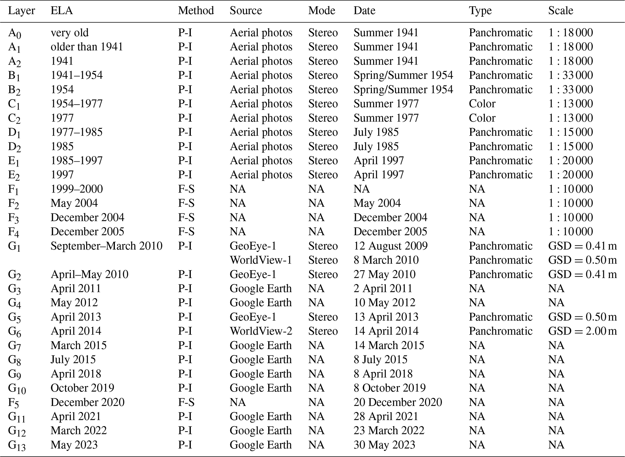
Figure 2 synthesizes the phases of the activities carried out to obtain the M-LIM-C. The first phase consisted in the acquisition of data, namely the identification of landslides. The investigation and identification of the landslides have been conducted using two methods: (i) image interpretation of aerial stereo-photographs (Galli et al., 2008), stereo satellite images (Ardizzone et al., 2013) and satellite images available on Google Earth Pro application; and (ii) field surveys conducted driving along the main and secondary roads and mapping landslides in the field at 1:10 000 scale using topographic base maps (Cardinali et al., 2006). In the last ten years the field mapping of the landslides was done taking notes directly on site using Google Earth, as described by Santangelo et al., 2023. The landslides observed in the field and delineated as polygons on Google Earth imagery, those identified through visual interpretation of very high-resolution (VHR) optical stereo satellite images and mapped directly on-screen (Ardizzone et al., 2013; Murillo-García et al., 2015), and those recognized through systematic inspection of the imagery available in Google Earth were mapped at a level of detail greater than that achievable at a 1:10 000 scale. This higher level of detail applies both to the minimum size of the mapped landslides and to the accuracy of the delineated polygon boundaries. Ardizzone et al. (2007) demonstrated that improved topographic information significantly enhances landslide identification and delineation. Consequently, the multi-temporal inventory is characterized by two different mapping scales. Until 2005, landslides were represented according to the cartographic scale of 1:10 000. After 2005, the effective mapping scale was controlled by the resolution of the VHR satellite imagery and Google Earth images used for landslide identification and mapping, resulting in a substantially finer level of detail.

The editing phase resulted in geometrically and topologically correct shapefiles (EPSG: 23 033), whose preparation methods have evolved over time in parallel with advancements in GIS software. Initially, in the early 2000s when aerial photography and digital stereoscopic viewing systems were not yet available, landslides were drawn by hand on transparent plastic sheets overlaid on paper stereoscopic aerial photographs and then transferred to 1:10 000 scale topographic base maps on additional transparent sheets, which were subsequently scanned for digital use (layers A₀ to E₂ in Table 1). With the advent of digital satellite imagery, landslides began to be delineated directly on the computer screen (layers G₁, G₂, G₅ and G₆ in Table 1) (Ardizzone et al., 2013, 2023; Galli et al., 2008). In the case of field surveys, shapefile production involved mapping landslides on-screen using digital raster topographic maps (1:10 000 scale), with field photographs aiding in the spatial positioning and in the characterization of the type and size of mass movements (Ardizzone et al., 2007; Cardinali et al., 2006). In recent years Google Earth was used to map directly landslides in the field to be converted into polygons in GIS once back in the laboratory (layers G₇–G₁₀, G₁₂ and G₆–G₁₄ in Table 1).

The final phase consisted in the implementation of the attribute table, based on a defined legend, after the control of the topology correctness. The final inventory includes 27 polygon shapefiles spanning from 1941–2023 and two polygon shapefiles related to landslides that are very old and old corresponding to a geomorphological inventory (A₀ and A₁ in Table 1).

The stereo paper aerial photographs used to compile the map span from 1941 through 1997, and range in scale from 1:13 000–1:33 000. A team of two geomorphologists carried out the interpretation of the aerial photographs. Each stereo pair was analyzed using a mirror stereoscope (4× magnification) and a continuous-zoom discussion stereoscope (3× to 20× magnification). Both instruments allowed simultaneous viewing and mapping of the same stereo pair by both interpreters. The interpreters used all morphological, geological and landslide information available from published maps, previous work carried out in the same area, and discussion with other geomorphologists. Care was taken to identify areas where morphology had changed in response to mass movements, and to minimize interpretation errors caused by land use changes or by differences in the viewing geometry of aerial photographs taken at different dates.

The recognition of geomorphological features from stereoscopic aerial photographs requires experience, training, a systematic methodology, and well-defined interpretation criteria (Zuidam and Zuidam-Cancelado, 1986). Photo interpreters classify geological objects and landforms based on their expertise and on the analysis of a set of diagnostic characteristics that can be identified in photographic imagery. These include shape, size, photographic color, tone, mottling, texture, pattern of objects, site topography and setting (Antonini et al., 2002; Murillo-García et al., 2015; Ray, 1960). Shape refers to the form of the topographic surface. Due to the vertical exaggeration of stereoscopic vision, shape is the most useful characteristic for the classification of an object from aerial photographs. Size describes the area extent of an object. Knowing the physical dimensions of an object is seldom enough for classification, but it can be very useful to identify properties such as extent and depth. Color, tone, mottling and texture depend on the light reflected by the surface, and can be used to infer rock, soil and vegetation types, the latter being a proxy for wetness. Mottling and texture are measures of terrain roughness and can be used to identify surface types and the size of debris. Pattern is the spatial arrangement of objects in a repeated or characteristic order or form and is used to infer rock type and resistance to erosion, as well as the presence of faults and other tectonic lineaments. Topographic site is the position of a place with reference to its surroundings. It reflects morphometric characteristics such as height difference, slope steepness and aspect, and the presence of convexities or concavities in the terrain. Setting expresses regional and local characteristics (lithological, geological, morphological, climatic, vegetational, and so on) in relation to the surroundings. Site topography and setting are particularly suited to inferring rock type and structure, attitude of bedding planes, and presence of faults and other tectonic features. Extensive field checks were conducted to check the landslides mapped.

In the GIS database, landslides attributed to a single date (e.g., a rainfall event) or period were stored separately. Following this procedure, new and active landslides recognized, e.g. in the 1977 aerial photographs were stored in a separate layer than the landslides mapped as inactive in the same photographs. In each of the five sets of aerial photographs used to prepare the inventory, we separated the landslides that appeared “fresh” (i.e., showing recent signs of activity) in the aerial photographs, from pre-existing or dormant landslides. Old and very old landslides (i.e., those occurring before 1941) are typically characterized by vegetation recolonization and by the dissection of the landslide topography by drainage networks (Cruden and Varnes, 1996). Landslides that occurred from 1941 onwards can be identified through the presence of scarps and deposit zones, as well as by changes in vegetation patterns. “Fresh” slope failures were assigned the date (i.e., the year) corresponding to the aerial photographs in which they were first identified (i.e. 1941, 1954, 1977, 1985, 1997). These “fresh” landslides are characterized by color, tone, and texture contrasts relative to the surrounding undisturbed terrain. The remaining slope failures (i.e., “non-fresh” landslides) were assigned to the time interval between two consecutive aerial surveys. Although these landslides no longer appeared fresh in the more recent imagery, they exhibited morphological changes relative to one or more of the earlier photo sets, indicating that they occurred during the inter-survey period (i.e. 1941–1954, 1954–1977, 1977–1985, 1985–1997). As a result, for a single set of aerial photographs, multiple layers were obtained “fresh or active” layer and “inter-period layer” (for example, the landslides identified fresh in the 1977 and 1954 aerial photographs are landslides that were probably triggered by an intense or prolonged weather event in the year of the photograph. These landslides are considered active landslides. The 1954–1977 inter-period landslides are landslides that were not present in the 1954 photographs and present but without apparent freshness in the 1977 photographs. These landslides likely were triggered by one or more intense or prolonged weather events during the period between l1 954 and 1977). The procedure required intensive and time-consuming GIS work to identify and correct topological and geographical errors, such as overlapping polygons, gaps between adjacent features, misalignments with base maps, and inconsistencies in attribute data. This step was essential to ensure the spatial accuracy and consistency of the landslide inventory over multiple temporal layers. The obtained GIS database stores information on landslides attributed to 11 different dates or periods including two layers referred to old and very old landslides, namely A₀ and A₁ which could be considered.

The inventory map obtained from the analysis of the aerial photographs was updated to include the period from 1998 onward through field surveys conducted after periods of prolonged rainfall. A high-resolution Digital Elevation Model with a ground resolution of 2 m×2 m was obtained through weighted linear interpolation of elevation points acquired by Airborne Lidar Swath Mapping. Acquisition of the elevation data was performed on 3 May 2004, following a rainfall period that resulted in numerous landslides. A reconnaissance field survey conducted immediately after the same rainfall period allowed mapping 70 landslides, Topographic derivative maps obtained from the digital elevation model were used to update the reconnaissance landslide inventory map in 22 selected sub-areas (Ardizzone et al., 2007). The results correspond to the F₂ layer in Table 1.

Starting in 2005, the use of satellite imagery – including very high resolution (VHR) stereo satellite images and the Google Earth platform – enabled near-annual updates of the inventory. The investigation of the VHR stereoscopic satellite images was conducted using the StereoMirrorTM technology for block orientation, and Stereo Analyst for ArcGIS^® SW for image visualization and landslide mapping (Ardizzone et al., 2013). The 3-D views of the topographic surface created with the oriented satellite images, were investigated to identify the landslides related to the rainfall that occurred in 2010, 2013 and 2014 years (G₁, G₂, G₅ and G₆ layers in Table 1). The digitalization of the landslides occurred simultaneously with the study of the stereo pair in a polygon shapefile. In the last ten years Google Earth Pro has provided imagery at nearly annual intervals. For years lacking aerial or satellite coverage, Google Earth was examined, and the available imagery was visually inspected. Landslides were digitized directly in KML format as polygons and subsequently converted into polygon shapefiles using GIS software (see Table 1 for the corresponding layers).

4 Multi-temporal landslide inventory map

The multi-temporal inventory includes 3700 landslides (Fig. 3) corresponding to an average density of about 46.8 landslides per square kilometer. The total landslide area is equal to 17.15 km², which represents 21.71 % of the study area. In this section the inventory will be analytically described. Section 4.1–4.3 describe landslides classified according to their relative age, type classification, and estimated depth (Cruden and Varnes, 1996). Landslide age, activity, and depth were determined based on the type of movement, the morphological characteristics and appearance of the landslides on the aerial photographs, the local lithological and structural setting, and the date of the aerial photographs.

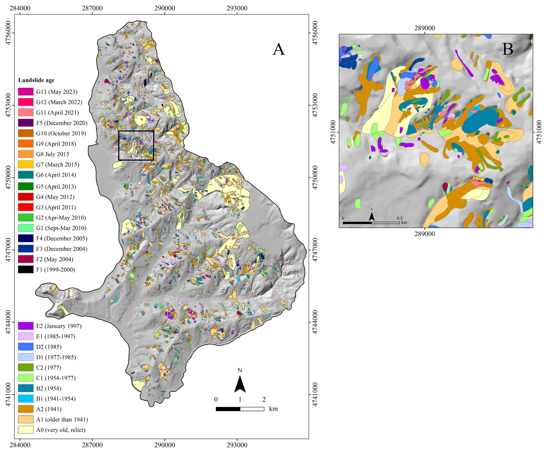
Figure 3 Collazzone study area: multi-temporal landslide inventory map. The landslides are represented by relative age. The black rectangle (A) shows the location of the enlargement of the map showing the abundance of the landslides over time (B).

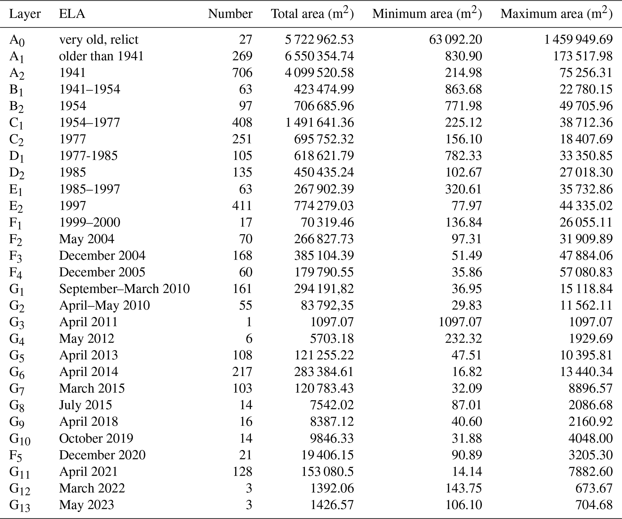
The smallest landslide area is equal to 14.14 m² and the maximum is equal to 1 459 949.70 m², the smallest landslide was identified in the Google Earth image taken on April 2021 (G₁₁ in Tables 1 and 2); the largest landslide was identified using aerial the photographs taken in 1941 (A₀ in Tables 1 and 2).

Table 2 Descriptive statistics of landslides by relative age. ELA: estimated landslide age. The letters from A to E indicate the layer prepared by the photointerpretation of the stereo-aerial photographs. The letter F indicates the layers prepared through field surveys. The letter G indicates the layer prepared using satellite imagery.

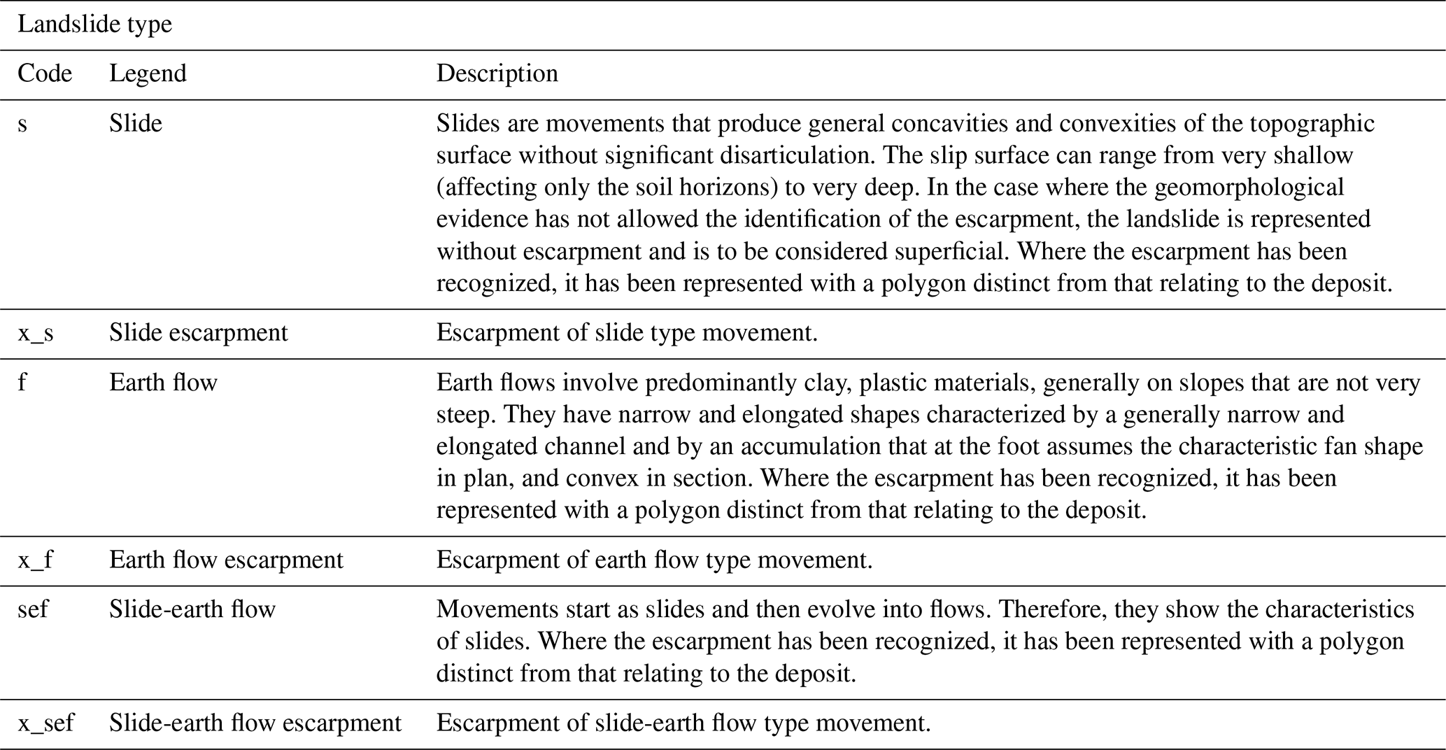
In the multi-temporal landslides inventory map each landslide is identified, in each layer, by a unique number. The attribute table of each layer includes three fields: N (identifier of each landslide); code (legend code); legend (extended legend of the code). Appendix A provides a data description and illustrates the explanation of the code and legend (Table A3).

In the following the classification criteria used to describe the landslides are illustrated: (i) age, (iv) type, and (iii) estimated depth.

4.1 Landslide by age

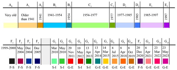
Based on their appearance in aerial photographs, landslides were classified according to their relative age, namely (i) very old relict landslides, (ii) very old landslides, (iii) landslides among two consecutive aerial photographs data, (iv) landslides active at the data of the aerial photograph, (v) landslides recognized in the field and dated considering the rainfall occurred immediately before the field survey and vi) landslides recognized in Google Earth images dated in the proximity of the image (Fig. 4). The four relative age levels (i), (ii), (iii) and (iv) refer to the general morphologic appearance of landslides (Keaton and DeGraff, 1996) and assume that evidence of landslides becomes less obvious with increasing age, due, for example, to erosion processes, vegetation growth, occurrence of other landslides or human activity such as example ploughing, excavation, urbanization and restoration. Hence, older landslides are more difficult to detect than more recent ones as described by Ardizzone et al. (2023).

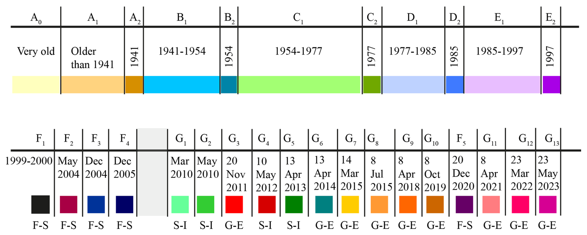
Figure 4 Timeline showing the age attributed at the landslide layers. See Table 1 for explanation of the layers. F-S means field survey, S-I means satellite image and G-E means Google Earth image.

In each of the five sets of aerial photographs, landslides that appeared “fresh” (i.e. active) on the aerial photographs were separated from the other landslides. The date (i.e., year) of the aerial photographs used to identify the landslides was assigned to the “fresh” landslides, while the period between two successive sets of aerial photographs was attributed at the other slope failures (i.e., the “non-fresh” landslides). It is worth noting that the exact or approximate age of the landslides is undetermined, and it is inferred to be intermediate between the dates of the aerial photographs used to identify the landslides. Event landslides were triggered by a known trigger (e.g., a rapid snowmelt event (Mauro Cardinali et al., 2000), a rainfall event (Ardizzone et al., 2007)) and were identified and mapped using a single set of aerial photographs taken shortly after the event (see layer E₂ in Fig. 5 and Table 1), or during a single field campaign. Event landslides pertaining to a single temporal layer of the inventory are of the same age, inferred from the date of the event, or the date of the aerial photographs or the field campaign. We started by identifying landslides on the 1954 aerial photographs (1:33 000) in comparison with the 1941 aerial photographs. The photographs taken in 1954 are suitable for the identification of landslides, because the flight took place before the intensive post-war agricultural exploitation in Italy and prior to the widespread reforestation that has since increased forest cover in Italy, then we analyzed the other sets of aerial photographs to prepare separate landslide inventory maps (Fig. 4 and Table 1).

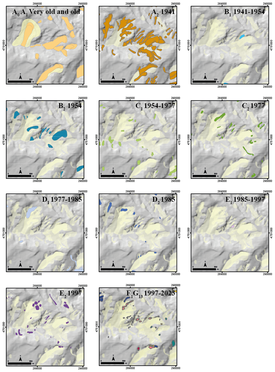
Figure 5 Enlargement of a portion of study area. The letters indicate the layers of the multi-temporal inventory map (Table 1 and Fig. 4). The panels show: (A₀A₁) very old and old landslides; (A₂) fresh landslides in 1941 photographs; (B₁) landslides occurred between 1941 and 1954; (B₂) fresh landslides in 1954 photographs; (C₁) landslides occurred between 1954 and 1977; (C₂) fresh landslides in 1977 photographs; (D₁) landslides occurred between 1977 and 1985; (D₂) fresh landslides in 1985 photographs; (E₁) landslides occurred between 1985 and 1997; (E₂) fresh landslides in 1997 photographs and (F₁G₁₃) landslides occurred from 1997 through 2023.

Figure 5 shows an enlargement of the M-LIM-C from very old (A₀), old (preexisting the 1941) in the panel (A₀A₁) to the landslides observed during the field surveys and using satellite tools (i.e. stereo satellite images and Google Earth images) after the 1997 in the panel (F₁G₁₃).

The Figs. 3 and 5 highlights that in the period of more of about 80 years (1941–2023) the temporal recurrence has high frequency and that landslides tend to occur where previous landslides occurred due to a legacy effect (Samia et al., 2017b).

4.2 Landslide by type

Landslide type included in the legend of the M-LIM-C are: (i) slide-type landslides (which include deep-seated slides and shallow soil slides), (ii) earth flow, (iii) slide-earth flow.

According to the type of movement, the most represented landslides in the study area are slides with 2830 landslides (example in Fig. 6a), whereas earth flows and slide-earth flows (examples in Fig. 6b and c) are represented by 515 and 355 landslides respectively.

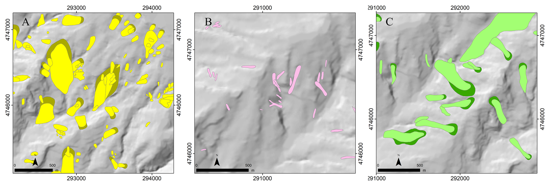
Figure 6 Enlargement of a portion of study area. Landslide examples of landslide type. (A) slide; (B) earth flow; (C) slide-earth flow.

The slides present a well-defined scarp which can be semi-circular (rotational slides) or angular (translational slides). The slide deposit is convex, with a morphologically depressed head of the deposit characterized by a centripetal drainage and local counter-slopes and a toe characterized by a typical upward bulge. Earth flows are characterized by an overall elongated planar shape, with the median part narrower than the detachment and accumulation zones. Slide-earth flows (Fig. 6c and d) start as slides and then evolve into flows. Therefore, they show the characteristics of slides (most commonly rotational) in the escarpment area and in the head of the deposit, on the other hand, the transport zone and accumulation zone are more like earth flows.

4.3 Landslide by estimated depth

The estimated depth of a landslide is assigned based on the main morphological characteristics of the landslide, such as slope height, and the extent of curvatures along the slope (convexity and concavity). Based on these morphological characteristics, landslides were classified as deep-seated or shallow. For deep-seated slope failures, the landslide crown was mapped separately from the deposit. The distinction was not made for the shallow landslides. Many of the deep-seated landslides can be classified as very old and older than 1941 landslides. They often involve considerable volumes of material and can alter the local morphology and geological structure. According to (Santangelo et al., 2015) the beddings condition the location and abundance of the deep-seated landslides, which are most abundant in cataclinal dip and under-dip slopes and does not condition significantly the distribution and abundance of the shallow landslides.

Figure 7 shows a deep-seated slide (A) and two shallow landslides (B and C).

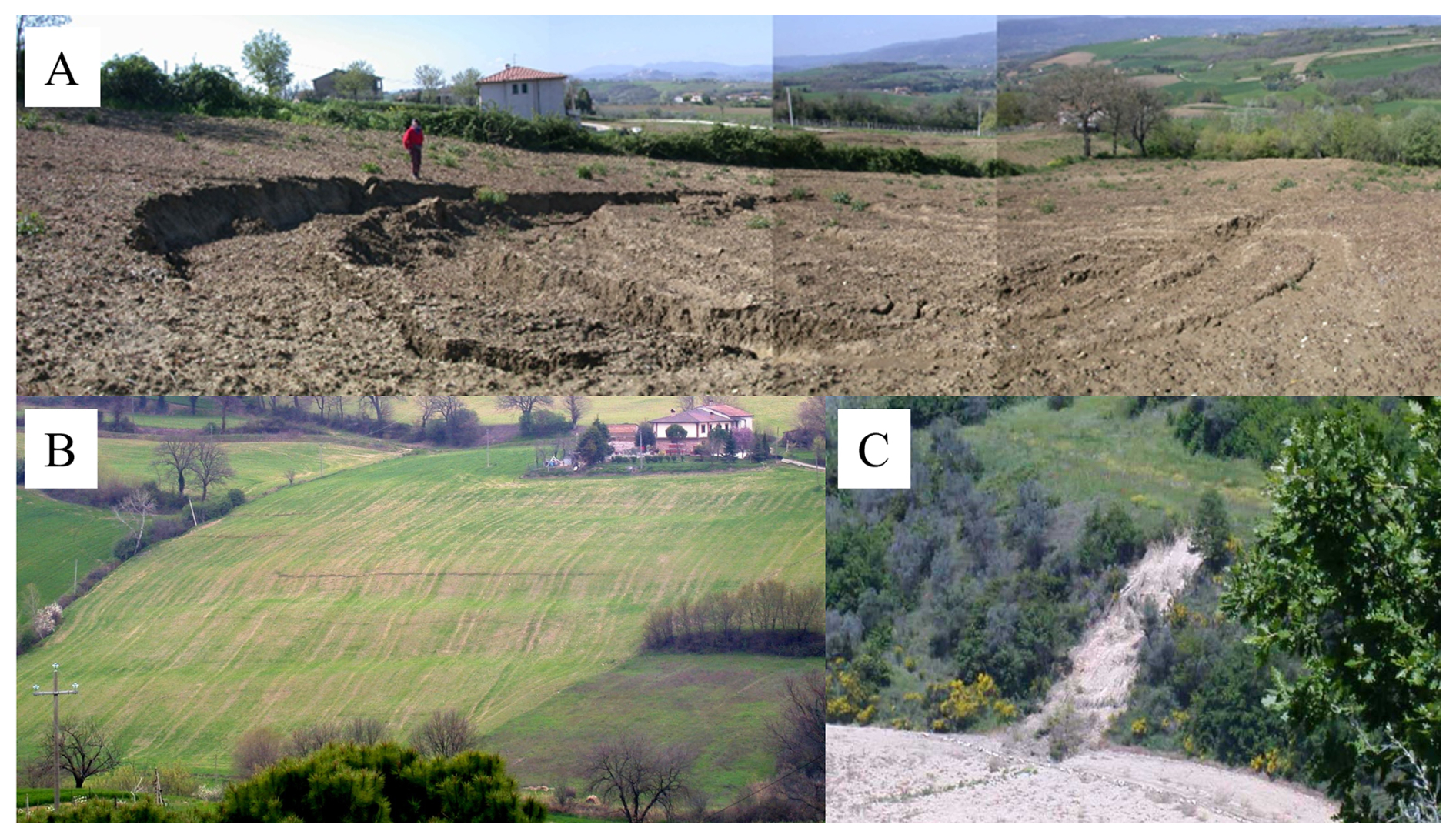
Figure 7 Examples of landslide depth. (A) deep-seated slide; (B) soil slide; (C) earth flow. The photographs were taken by the CNR- IRPI.

4.4 Descriptive statistics

Descriptive statistics in number and size (total, maximum and minimum area) of the landslides are shown in Table 2 and in the box plots in Fig. 8a and b. Figure 8 shows the distribution of landslide areas for the landslides based on the age grouped on four classes of age: (i) very old (relict) landslides; (ii) old landslides (landslides occurred before 1941); (iii) recent landslides (landslides occurred between 1941 and December 2005) and (iv) current landslides (occurred after December 2005). Figure 9 shows landslide count (represented by a color gradient and labels) and cumulated area (proportional to circle sizes), grouped by relative age class and landslide type.

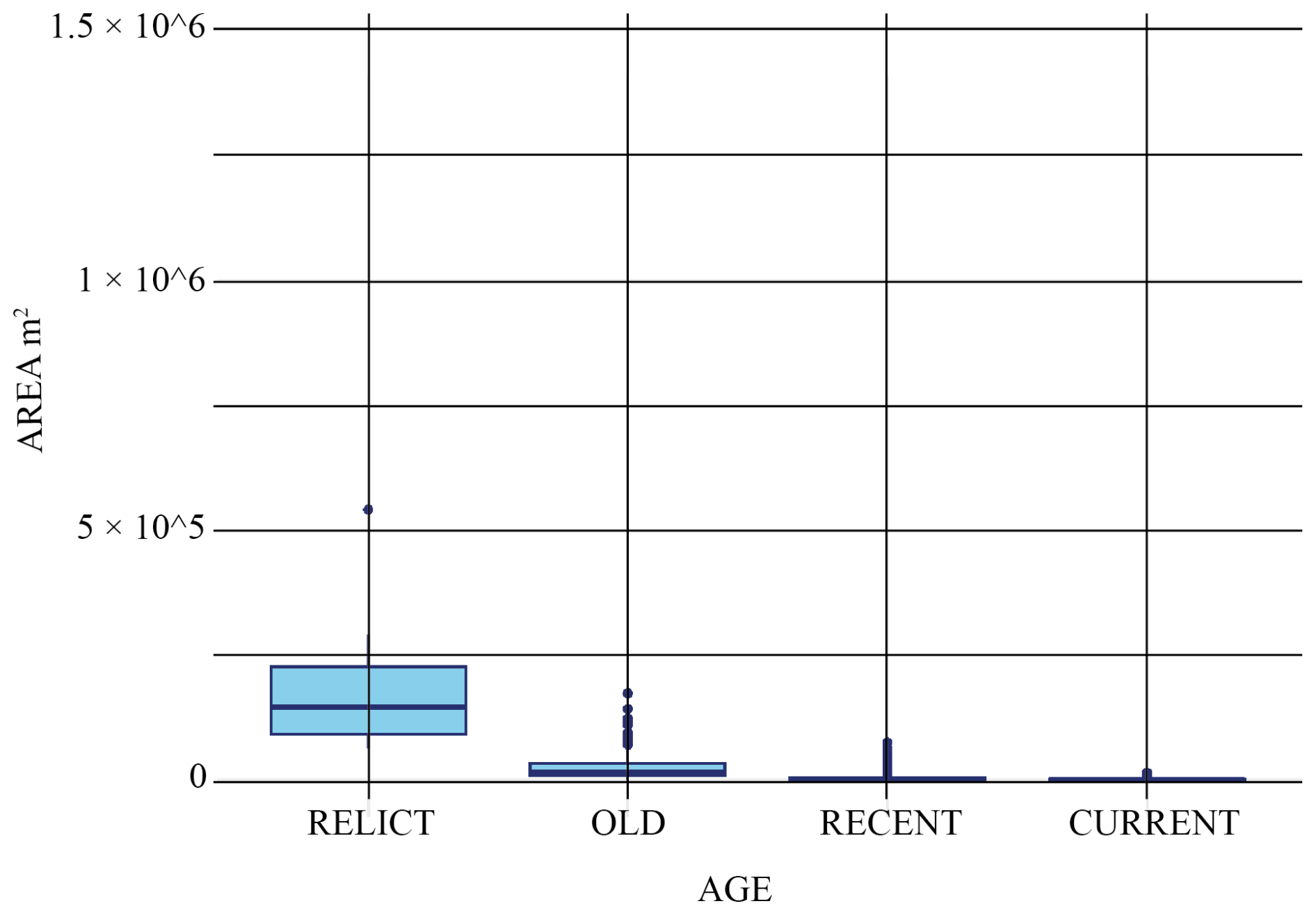
Figure 8 Plots summarizing landslide statistics. Landslide area grouped by relative age class (relict; old; recent and current).

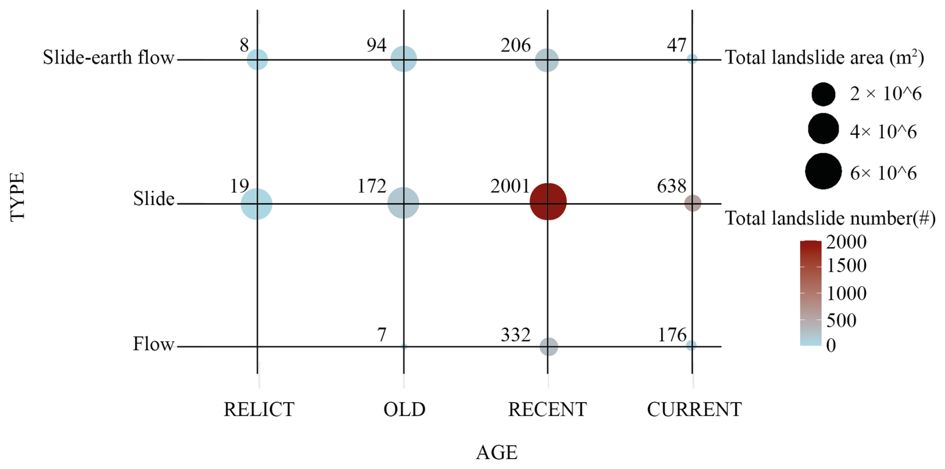
Figure 9 Scatterplot showing cumulative sizes and counts of landslides grouped by relative age in the abscissa and type in the ordinate. Landslide number is represented by a color gradient and labels; total area is proportional to circle sizes. The number on the symbols represents the number of the landslides.

The plot in Fig. 8 shows the size distribution of the four groups of landslides. The clear separation of the age groups according to their median values indicates that relict and old landslides have a median value higher than the median of recent and current landslides. That could be an indication that relict landslides were triggered in a different tectonic and climatic setting while recent and current landslides were triggered in a similar climatic setting. As far as concern the old landslides, probably they have triggered in a climate environment different from the others.

Figure 9 shows landslide count (represented by a color gradient and labels) and cumulated area (proportional to circle sizes), grouped by relative age class and landslide type. Visual inspection of the plot reveals that relict and very old landslides are mainly represented by small landslides represented by flows which tend to be small and easily obliterated by erosion and subsequent failures. Further evidence is that a large portion of the total landslide area is occupied by few relict landslides, whereas the smallest landslides correspond to the current period, according to the results by Ardizzone et al. (2023). They suggested that a size threshold effect of previous landslides on subsequent landslides.

5 Quality control

The quality of a landslide inventory depends on its accuracy and the type and certainty of information shown on the map. Defining the accuracy of a landslide inventory is not straightforward, and there are no standards (Galli et al., 2008). Accuracy depends on the completeness of the map and the geographic and thematic correctness of the information displayed on the map. Galli et al. (2008) compared the landslide inventory map of Collazzone area, including landslides until 2005, with two pre-existing landslide inventory maps for the same study area: a reconnaissance landslide inventory map and a geomorphological landslide inventory map (namely A1 and A2) prepared by photo interpretation of one and three sets of stereo aerial photographs respectively and very few field checks. The first test consisted of evaluating the degree of cartographic matching between the maps, comparing the inventories in pairs in a GIS. The overall error index (E) was calculated according to Ardizzone et al., 2002, using the equation (Eq. 1):

$$\begin{array}{}\text{(1)}& E={\displaystyle \frac{(A\mathrm{1}\cup A\mathrm{2})-(A\mathrm{1}\cap A\mathrm{2})}{A\mathrm{1}\cup A\mathrm{2}}},\text{with}E\mathrm{0}\le E\le \mathrm{1}\end{array}$$

where A1 and A2 are the total landslide areas in the first and in the second inventory, respectively, and ∪ and ∩ are the geographical union and intersection of the two inventories, obtained in a GIS.

Mapping error ranges from 0.66–0.81, the overall mapping error is smallest (0.66) when the most accurate (landslide inventory) and the second most accurate (geomorphological inventory) inventories are compared. The error includes: (i) uncertainties associated with the identification of the landslides, (ii) drafting and positional errors introduced when transferring the landslide information from the aerial photographs to the base map, (iii) digitization errors and other mistakes introduced in the construction of the digital cartographic database (Carrara et al., 1992). Moreover, the authors evaluated the drafting and digitization errors from the mismatch due to different geomorphological interpretations, the figures correspond to a cartographic error of approximately 2.5 %–5 %. The remaining mismatch (∼62 %–75 %) was attributed to different geomorphological interpretations. The authors determined the frequency-area statistics of landslides and probability density function (pdf) obtained for the three landslide inventory maps differ significantly. The area of the most abundant landslides of the inventory is 815 m² that is less than the other two inventories, and the power-law exponent is also less than the other two. These figures indicate that the landslide inventory map contains a very large number of small landslides.

To validate the landslides defined “current landslides” occurred after the 2005 an external geomorphologist investigated four geographical sectors, shown in Fig. 10, using Google Earth. Landslides from 2013, 2015, 2018, 2019, and 2021 were identified in sectors 1, 3, and 4. In sector 1 the geomorphologist didn't recognize any landslide.

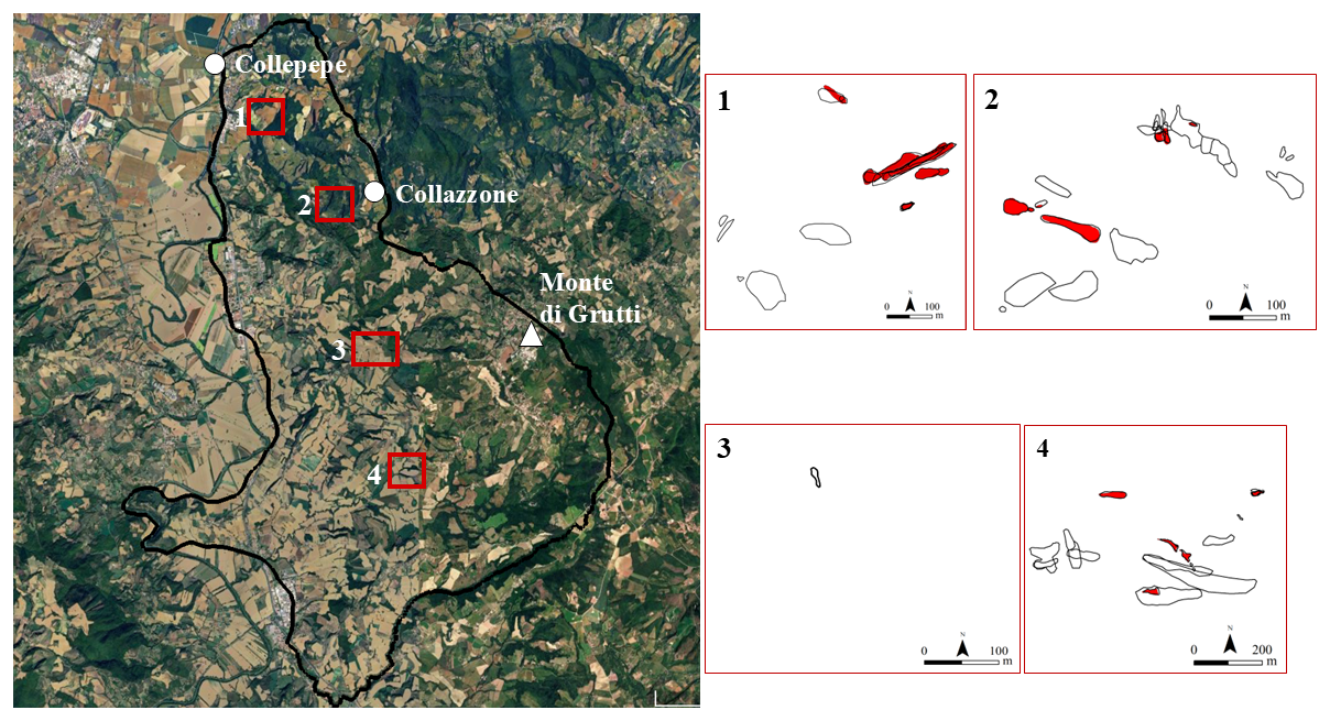
Figure 10 Collazzone study area: localization of the four geographical sectors. Map data: © Google Earth 2026, Imagery: © 2026 Airbus. An independent geomorphologist investigated the images of different times in the four sectors. In the four sectors black lines show the landslides included in the multi-temporal landslide inventory map. Colored polygons represent the landslides mapped by the external geomorphologist.

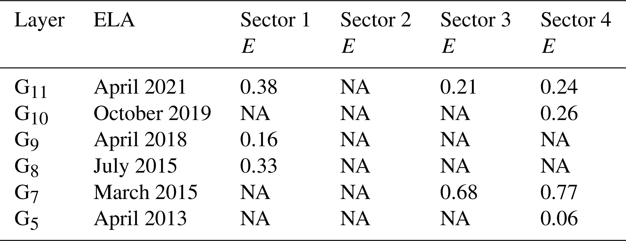
To analyze quantitatively the differences between the two inventories the overall error index (E) was calculated between landslides belonging to the same date. The results are shown in Table 3. The overall error index varies between 0.06 and 0.77.

Table 3 Overall error Index (E) calculated in four sectors of the study area (Fig. 10). The values were calculated between the landslides of the multi-temporal landslide inventory and the landslides identified by the external geomorphologist who had investigated Google Earth Images along time. ELA: estimated landslide age. NA means not applicable.

6 Data availability

The dataset is available in a Zenodo repository: https://doi.org/10.5281/zenodo.18980281 (Ardizzone, 2026).

7 Conclusion

The multi-temporal landslide inventory map presented in this paper is the result of mapping work that began around the year 2000. Even today, landslides in the Collazzone area are identified following intense or prolonged meteorological events. The landslide inventory was produced in the framework of free scientific research initially to deepen knowledge from a geological and geomorphological point of view of a hilly area intended mainly for agricultural use to reconstruct the evolution of the landscape. During the preparation of the inventory map, it became clear that this information could be used to develop models for zoning landslide hazard and risk.

Galli et al. (2008) established that the multi-temporal inventory in Collazzone represents a significant improvement upon the geomorphological and reconnaissance inventories. In this work the authors proposed a framework for a quantitative comparison of landslide inventory maps through several tests. However, due to the time and the resources required to complete an inventory, such type of detailed mapping cannot be effectively prepared for a large region, extending for thousands of square kilometers, even though any landslide hazard evaluation requires considering the temporal behavior of the landslides. For the current landslides a comparison between the landslides of the multi-temporal landslide inventory and the landslides identified by the external geomorphologist in four sectors was carried out. Findings revealed an overall index error ranging from 0.06–0.77.

The availability of this inventory (Ardizzone, 2026) has enabled many researchers from international institutions to conduct research curiosity driven as proved by numerus published papers (Samia et al., 2020; Lombardo et al., 2020; Samia et al., 2018, 2017a; Rossi et al., 2010; Samia et al., 2017b; Guzzetti et al., 2009b; Galli et al., 2008; Guzzetti et al., 2006a, b).

Appendix A: Data description

The digital multi-temporal landslides inventory map is composed of 29 polygon shapefiles (Table A1). The EPSG is 23033. The attribute table of each shapefile includes three fields, beyond the default fields: N, CODE and LEGEND (Table A2). Table A3 shows the legend of the types of landslides.

The 29 shape files named as the layer in Table 1 and the corresponding geopackage named “Landslide_inventory_Collazzone.gpkg” are available in ZENODO repository (https://doi.org/10.5281/zenodo.21531647, Ardizzone, 2026).

Table A1 Shapefiles included in the multi-temporal landslide inventory map. P-I: Photo Interpretation; F-S: Field Survey; S-I-I: Satellite Image Interpretation; G-E-I: Google Earth Image interpretation.

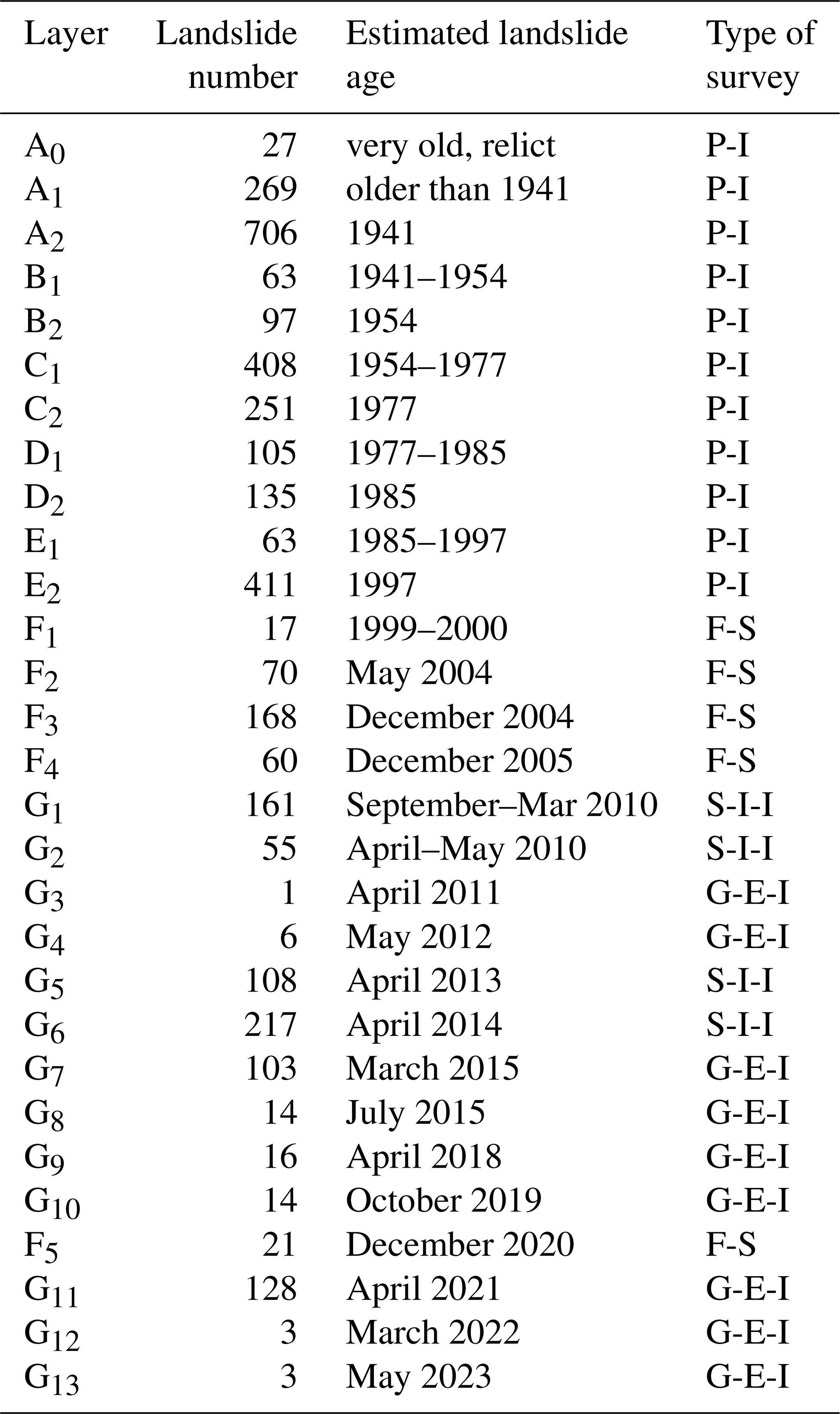
Table A2 List of the fields included in the attribute table of each shapefile of the multi-temporal landslide inventory map of Collazzone study area. The table includes three fields beyond the default fields: N, CODE and LEGEND.

Table A3 Legend according to Cruden and Varnes (1996).

Appendix B: Monthly cumulative rainfall (from 1940–2023)

The graph (Fig. B1) shows the monthly cumulative rainfall (mm) measured at Todi rain gauge (Fig. 1a) from 1940–2023. The red line indicates the average annual rainfall equal to 72 mm. The black dots A₂, B₂, C₂, D₂, and E₂ show the date of the stereophotographs. The black dots F₁, F₂, F₃, F₄ and F₅ show the date of the field surveys. The black dots G₁, G₂, G₅ and G₆ show the date of the very high-resolution satellite images. The black dots G₃, G₄, G₇, G₈, G₉, G₁₀, G₁₁, G₁₂ and G₁₃, show the date of the Google Earth Pro images.

Figure B1 Monthly cumulative rainfall (mm) measured at Todi rain gauge (Fig. 1A) from 1940–2023. Red line indicates the average annual rainfall (72 mm) the black dots show the date of the inventory layers.