the Creative Commons Attribution 4.0 License.
the Creative Commons Attribution 4.0 License.
 | 27 Jul 2026

The rainfall and erosivity database for Mexico (1968–2017)
Viviana Marcela Varón-Ramírez
Douglas Andrés Gómez-Latorre
Carlos Eduardo Arroyo-Cruz
Alberto Gómez-Tagle
Blanca Lucía Prado Pano
Ronald R. Gutierrez
Deyanira Lobo-Luján
Mario Guevara
Soil water erosion is the dominant soil degradation driver worldwide. Rainfall erosivity (also known as the R factor) quantifies the potential of rainfall to cause soil water erosion and is regarded as a dominant factor determining it. This contribution presents the first annual R factor database across the continental Mexico for three climate normals (1968–1997, 1978–2007, and 1988–2017). The workflow comprised three main steps. Firstly, a harmonaized daily rainfall time series dataset was obtained by compiling and harmonizing (through quality control, homogeneity analysis and gap-filling) 5410 raw rainfall time series distributed across Mexico. Secondly, three combinations of the α and β coefficients in a power model were tested to estimate daily R factors using three validation databases at global, national, and local scales. Thirdly, a validated and continuously distributed annual R factor for all three climate normal was obtained. Thus, the database presented herein encompasses 1369 (climate normal 1968–1997), 1678 (climate normal 1978–2007), and 1676 (climate normal 1988–2017) rainfall time series and the corresponding R factor. Our results indicate that the median values of the R factor for the three climate normals were 3245; 3070; and 3327 MJ mm ha−1 h−1 yr−1, respectively. The statistical distribution of the R factor is right-skewed for the three climate normals, with high erosivity values reaching >12 000 MJ mm ha−1 h−1 yr−1 in all cases. The R factor across Mexico showed a strong ecoregional differentiation, with the highest values concentrated in the Tropical Rain Forest and Tropical Dry Forest ecoregions, whereas the North American Deserts and Mediterranean California exhibited the lowest values. The annual behavior of the R factor was similar for the three climate normals. However, September had the highest contribution to the annual R factor. By identifying areas with higher susceptibility to soil loss due to rainfall action and providing spatially distributed and well-documented estimates, we believe that the present R factor database has the potential to support the study of soil water erosion in the continental Mexico at country scale. Said database is available from a scholarly-accepted repository at https://doi.org/10.6073/pasta/dd2b30e28ee25ff2d60d8a9f436951d2 (Varón-Ramírez et al., 2026) for public consultation.
- Article
(12298 KB) - Full-text XML
- BibTeX
- EndNote


Soil water erosion (SWE) refers to the soil displacement from its original location due to water action, such as rainfall, overland flow, and irrigation (Nearing, 2013). SWE represents the dominant soil degradation issue at the global scale because it affects nearly 33 % of the World's surface (Pennock, 2019). SWE has both on-site and off-site effects. On-site, soil loses its natural capacity to store water, nutrients, and organic carbon (Hatfield et al., 2017), affecting, for instance, food security. Off-site, the eroded soil triggers environmental issues such as water pollution, dam siltation, eutrophication of water bodies, contamination of coastal and marine ecosystems, and overall environmental damage (Feng et al., 2023; Borrelli et al., 2022; Guo et al., 2020). These widespread impacts underscore the urgent need to study SWE at national scales to guide effective land and water management, especially in tropical countries (Rosas and Gutierrez, 2020; Varón-Ramírez and Guevara, 2024).
Rainfall erosivity is the potential of rainfall to cause SWE (Nearing et al., 2017). Research evidence shows that rainfall erosivity is the dominant factor influencing SWE. As extreme rainfall events are expected to increase in frequency and intensity in tropical zones, rainfall erosivity is also expected to rise (Borrelli et al., 2020). Mexico is exhibiting this pattern as the temporal distribution of rainfall has become more extreme, with longer droughts and increasingly severe rainfall events (Porrúa et al., 2020). Thus, understanding rainfall erosivity patterns across Mexico and analyzing them over a multi-year period is essential for enhancing soil sustainability and informed decision-making in soil conservation at national scale.
Rainfall erosivity, often represented as the R factor, captures the combined effect of raindrop impact and water flow. Wischmeier and Smith (1958) defined the rainfall erosivity of a storm as energy × times × intensity (EI). The E term refers to the total storm energy, and the I term refers to the maximum 30 min intensity I30. The R factor is commonly expressed as the EI30 index, and over multi-year period, the R factor represents the mean annual rainfall erosivity, and the yearly rainfall erosivity (Ry) results from totaling the rainfall erosivities for all storms in a year. Several studies have shown that higher-resolution data (e.g., minute-resolution) yield more accurate erosivity estimates for a specific time period (Yin et al., 2015). High-resolution rainfall data is however challenging to obtain, especially for national-scale analyses in developing countries (Rosas and Gutierrez, 2020). Consequently, a common approach in these contexts is to construct empirical relationships of erosivity based on insufficient finer-resolution rainfall data and/or long coarse-resolution rainfall data (e.g., daily, monthly, and annual).
Mexico lacks a public database of high-temporal-resolution (i.e., sub-hourly) rainfall time series. The existing data is incomplete and has breakpoints pitfalls that limit studying climatic-related processes at national scales (Cuervo-Robayo et al., 2020). Thus, SWE-related studies have computed the R factor using coarse-resolution rainfall time series (monthly or annual) for specific regions (Benites et al., 2020; González et al., 2016) and/or developed empirical relationships using daily rainfall to approximate EI30. The Mexican Meteorological Service provides a rainfall database (daily records from approximately 5,454 weather stations across Mexico, with time series spanning heterogeneous periods from 1900 up to 2020), which opens up the opportunity to study the national rainfall erosivity patterns.
Several models have been developed to estimate the R factor worldwide. For instance, Richardson et al. (1983) proposed a power law model by assuming that a daily rainfall could be interpreted as a single storm. This model has been used in several countries to describe rainfall erosivity patterns (Rutebuka et al., 2020). Said model nevertheless requires sufficiently long time rainfall series (e.g., at least 20 years) to capture seasonal variability and mitigate cyclical rainfall biases (Kumar et al., 2026). Therefore, access to harmonized, quality-controlled, and sufficiently long rainfall datasets is critical for users aiming to perform consistent soil erosion modeling based on the R factor and environmental assessments at regional and national scales.
The main objective of this contribution is to address the requirements for consistent and reliable model inputs to assess the impact of precipitation on SWE at national scale in Mexico. To this end, two specific objectives are defined, namely (a) to construct the first harmonized rainfall database for three climate normals (1968–1997, 1978–2007, and 1988–2017) derived from legacy climate data, and (b) to construct the first rainfall erosivity estimates across continental Mexico. Section 2 of this article elaborates on the methodological aspects of (1) development of the daily rainfall time series database, (2) identification of the best empirical relationship to estimate daily rainfall erosivity, and (3) estimation of the rainfall erosivity across Mexican territory. The results (Sect. 3) are then presented accordingly, and, subsequently, discussed through a critical analysis based on recent scientific literature in Sect. 4. We finally present our conclusions in Sect. 5. All the computational codes and resulting databases of this research are freely available from a scholarly-accepted repository. We believe that these products provide a basis for improving the understanding of rainfall distribution and its role in soil erosion processes across Mexico.
The study area corresponds to continental Mexico (1 948 170 km2), which is located between latitudes 14 and 32° N and longitudes 86 and 118° W. Mexico exhibits complex climatic features influenced by subtropical high-pressure systems over the North Atlantic and northeastern Pacific, as well as its position relative to the Intertropical Convergence Zone (de Anda Sánchez, 2020). Mexico has been clustered into seven first-level ecoregions, which represent geographical units with characteristic biodiversity (Commission for Environmental Cooperation, 1997), namely: Mediterranean California, North American Deserts, Semi-arid Elevations, Great Plains, Tropical Rain Forest, Tropical Dry Forest, and Temperate Sierras. Each ecoregion occupies 1.3 %, 28.6 %, 11.8 %, 5.5 %, 14.2 %, 16.4 %, and 22.3 % of the total country area, respectively (Fig. 1).
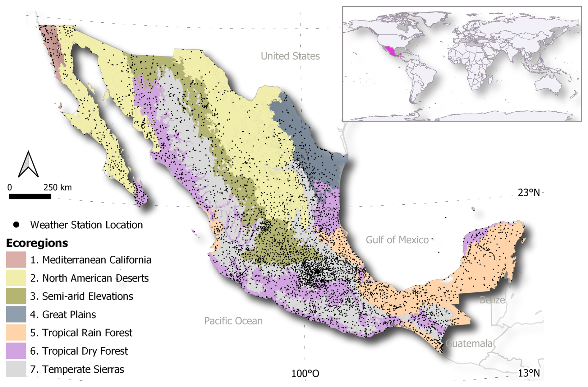
Figure 1Ecoregions defined by the Commission for Environmental Cooperation (1997) and locations of the weather station available from the Mexican Meteorological Service.
This research followed a workflow of three methodological stages (Fig. 2). First, we developed a rainfall time series database at daily resolution. Second, we identified the best empirical relationship to estimate erosivity using daily rainfall data. Third, we estimated the rainfall erosivity by using daily rainfall time series across the entire Mexican territory.
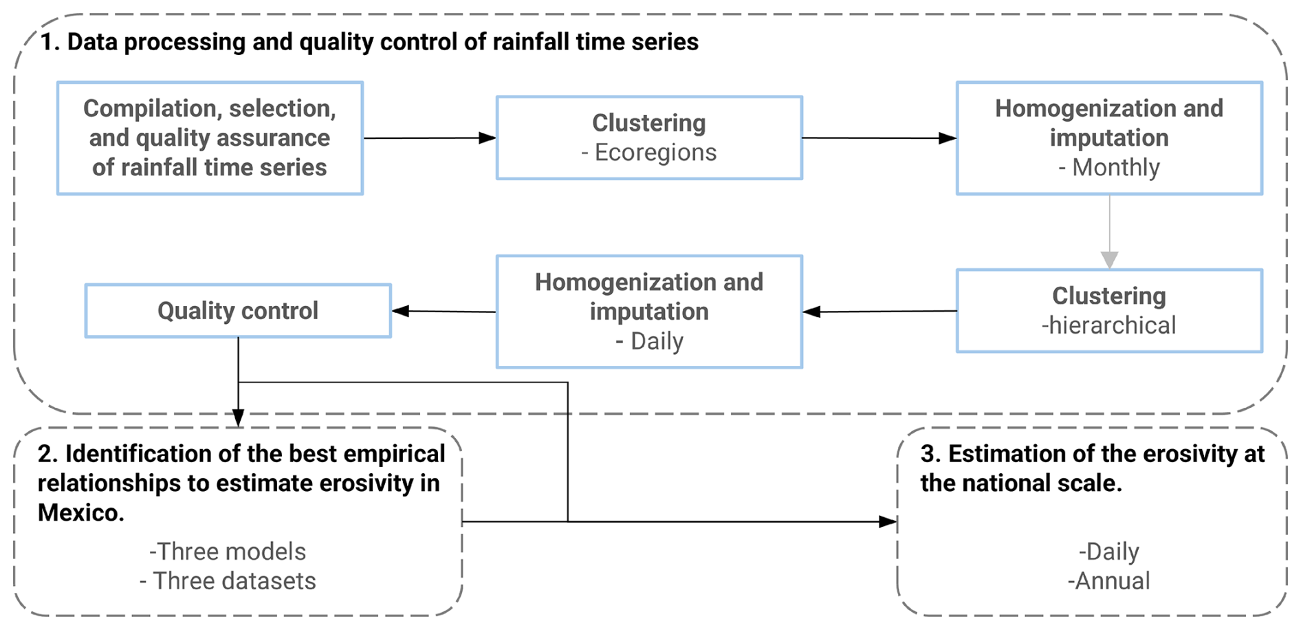
Figure 2Workflow summarizing the three key methodological stages: (1) development of the rainfall series database, (2) identification of the best empirical relationships to estimate erosivity in Mexico, and (3) estimation of the erosivity at the national scale.
2.1 Data processing and quality control of rainfall time series
Developing a rainfall time series and, subsequently, a rainfall erosivity database is challenging in both spatial and temporal terms. The large diversity of topographic conditions (i.e., two principal mountain ranges and a large latitudinal extent) and proximity to large water bodies from the Pacific Ocean and the Gulf of Mexico make Mexico a contrasting scenario for rainfall patterns (Carrera et al., 2024) and hydrological-related processes (e.g., rainfall erosivity). Accurate benchmarks for understanding typical climate conditions and characterizing climate trends require a rainfall database long enough to represent its corresponding climate normal (CN), i.e., a statistical product computed over 30 years of rainfall time series (WMO, 2017). The CNs are widely used to compare recent observations, create anomaly-based datasets, and provide context for future climate projections. Considering local patterns across different CNs, these characteristics will contribute to an unprecedented rainfall time series dataset for estimating rainfall erosivity in Mexico.
On the other hand, climatology studies, such as erosivity, need a complete and reliable rainfall time series database (Yozgatligil et al., 2013). Therefore, a whole scheme of quality assurance, gap-filling, and homogenization process of the rainfall time series is needed (WMO, 2023). This quality control and homogenization process has been widely applied before rainfall erosivity analysis, in order to avoid incoherent rainfall amounts that could affect the long-term rainfall erosivity estimates (Rutebuka et al., 2020). Consequently, with a reliable rainfall database, it is possible to represent the actual rainfall characteristics in a particular region and allow soil erosion monitoring at the local and national scales in Mexico.
The rainfall time series database was developed through four steps: first, compilation, selection, and quality assurance of the rainfall time series. Second, the clustering of the rainfall time series based on their geographical and data attributes. Third, homogenization and data gap-filling of monthly and daily rainfall time series. Fourth, quality control of the data gap-filling process.
2.1.1 Compilation, selection, and quality assurance of rainfall time series
The data were downloaded from the official National Meteorological Service website (https://smn.conagua.gob.mx/es/, last access: 4 April 2026) in January 2022. For this project, 5454 plain-text files were downloaded, corresponding to the daily database of the entire network of weather stations (Fig. 1). After a harmonization process, 44 plain-text files without rainfall data were discarded. Finally, a set of 5410 daily rainfall time series was obtained for use in this study.
Although the database includes records with an emission date extending to June 2020, inspection of the rainfall time series indicates that the period with the most complete and consistent data spans from 1961 to 2017. On the other hand, for erosivity estimates, it is recommended to use a historical rainfall time series of ≥20 years (Vantas et al., 2019; Renard and Freimund, 1994). Therefore, this study analyzed the rainfall time series in three climate normals: CN1 (1968 to 1997), CN2 (1978 to 2007), and CN3 (1988 to 2017).
Subsequently, we selected rainfall time series with less than 20 % missing values (WMO, 2023), resulting in 1489, 1785, and 1728 rainfall series for CN1, CN2, and CN3, respectively (Table A1). However, long sequences of zeros and missing values (NAs) were frequently identified within the selected rainfall series. Therefore, as part of the quality-assurance procedure, zero sequences ranging from three to six consecutive years were considered suspicious and replaced with NAs. Additionally, rainfall time series containing zero sequences longer than six years were discarded from the analysis (10, 11, and 7 rainfall time series for CN1, CN2, and CN3, respectively). After applying these filters, the final dataset comprised 1479, 1774, and 1721 rainfall time series for CN1, CN2, and CN3, respectively.
2.1.2 Clustering of rainfall time series
Clustering analysis is highly recommended when gap-filling a large set of rainfall time series (Guijarro, 2014). Clustering similar rainfall time series enables leveraging information from related series to fill in gaps. Rainfall patterns often exhibit spatial and temporal correlations, so data gap-filling from a group of similar series can result in more accurate estimates (Fransiska et al., 2024). In this workflow, we performed data gap-filling by clustering rainfall time series according to (1) ecoregions and (2) data dissimilarity across different environments (Fig. 2). The first clustering was performed using the ecoregions of North America (Commission for Environmental Cooperation, 1997; INEGI-CONABIO-INE, 2008). The second clustering was applied after gap-filling and homogenization of the monthly series within each ecoregion, using hierarchical clustering to group time series with similar seasonality and rainfall-volume patterns (Gómez-Latorre et al., 2022). The number of clusters (k) ranged from 2 to , where n is the total number of stations in the dataset (Rohlf, 1974). The better k values for each ecoregion were found using the Hartigan cluster validation index (Hartigan, 1975). This index was identified by Todeschini et al. (2024) as performing better than 68 cluster validation indexes across 21 datasets. However, we did not perform a clustering analysis for the Mediterranean California and Great Plains ecoregions due to their small size and the limited rainfall time series available for those ecoregions.
2.1.3 Homogenization, data gap-filling and quality control of the rainfall time series
We followed three steps to get a complete rainfall time series for each CN: quality assurance, homogeneity analysis, and data gap-filling (WMO, 2020). In this step, quality assurance involved verifying the physical and statistical consistency of the series, discarding outliers whose standardized anomaly was outside a predefined threshold and was unrelated to any climate variability events. Outliers were removed and replaced with NA values to be filled during the data gap-filling process.
Homogeneity analysis removes the biases caused by some artificial breaks in the rainfall time series (Yan et al., 2014). These breaks result from common issues such as reading or measurement errors, instrumental changes, or atypical situations at the weather station location (Guijarro, 2014). We used the standard normal homogeneity test (Alexandersson, 1986) to analyze homogeneity.
To fill in missing data, we used the proportions method. This method estimates the missing information based on neighboring stations, considering the distance between each station (Paulhus and Kohler, 1952). The procedure used the three precipitation series with the highest correlation coefficient to the series that will be filled, with the condition of having been previously normalized. Then, we estimated ; where Na, Nb and Nc are the precipitation data for each of the stations with the highest correlation, while Aa, Ab and Nc are their corresponding normal average. All of the data gap-filling and homogenization process was made with the homogen function of the climatol R package (Guijarro, 2024). We summarized the homogenization parameters used for each step. Table A2 shows the parameters used to homogenize the monthly series, while Table A3 shows the parameters used to homogenize daily series by ecoregions 2, 3, 5, 6, and 7 and their corresponding subgroups.
A quality validation was performed using the McCuen test (McCuen, 2016) to ensure consistency during the data gap-filling process of the rainfall time series. McCuen test compares the differences between the aggregated rainfall of the original multi-annual monthly means and the final series. The generated rainfall time series with a difference greater than 10 % related to its original was discarded.
Finally, to evaluate the effect of the gap-filling procedure on rainfall climatology, we calculated the root mean square error (RMSE) between the mean monthly precipitation of the original incomplete series and the corresponding completed series after gap filling. RMSE was calculated for each weather station and subsequently summarized by ecoregion and climate normal. This metric quantifies the deviation in the monthly climatological behavior introduced by the gap-filling procedure. Therefore, RMSE provides an indicator of the sensitivity of rainfall regimes to missing data completion across different climatic regions.
2.2 Identification of the best empirical relationships to estimate erosivity in Mexico
In this step, we identified the best empirical relationship to calculate the R factor according to the erosivity characteristics of Mexico. To achieve this, we evaluated three combinations of parameters α and β in a power law model and used three databases with EI30 information on a global (Panagos et al., 2023), national (Cortés, 1991), and local (EI30 calculated from sub-hourly rainfall time series) scale.
2.2.1 Empirical relationships to estimate daily erosivity
The empirical relationship follows the power-law model proposed by Richardson et al. (1983) when using daily precipitation to estimate the daily erosivity Rd (Eq. 1). When comparing rainfall erosivity estimates using power and linear models, power models perform better when applied to daily rainfall time series in tropical and subtropical zones (Rutebuka et al., 2020; Karami et al., 2012)
where Pd is the daily precipitation, α, and β are the adjusted coefficients. We tested three combinations (Model I, II, and III) of adjusted coefficients as follows:
-
Model I (Richardson et al., 1983): the value of α is equal to 0.18 for the cool season (October to March) and 0.41 for the warm season (April to September). The value of β is equal to 1.81 and constant throughout the year.
-
Model II (Liu et al., 2020): the value of α and β variate depending on the climate zone according to the Koppen–Greig Classification as follows: for Tropical (A), , and . For Arid-steppe (BS), β=1.73 and α=0.3296. For Arid-desert (BW), β=1.514 and . For Temperate with dry summer (Cs), β=1.563 and α=0.2735. For Temperate with dry winter (Cw), β=1.558 and α=0.817. Finally, for Temperate with dry winter (Cf), β=1.5 and . To identify the climate classification at each location of the datasets, we used the Koppen–Greig Classification for the present (1980–2016) at 1 km of spatial resolution made by Beck et al. (2018).
-
Model III (Xie et al., 2016): the value of α is equal to 0.2686. The value of β is equal to 1.7265. This model also includes a sinusoidal relationship to describe the annual cycle of the coefficient of the power law function to represent seasonal differences in rainfall characteristics (Eq. 2) as proposed by Yu and Rosewell (1996).
where f is the monthly frequency (); ω is ; η is 0.5412; and j is the j-month of the year.
2.2.2 Databases containing EI30 information
We used three databases to evaluate the performance of the three models described earlier. Two compiled databases provide EI30 values directly: a global dataset developed by Panagos et al. (2023) and a national dataset derived from the Master's thesis of Cortés (1991). In addition, a local database was included to enable model performance at a finer scale in Mexico. This third database corresponds to the Michoacán Region and was constructed using sub-hourly (15 min) rainfall time series from which EI30 was calculated. These three validation databases have a different statistical distribution of the EI30 factor (Fig. A1), displaying a wide range of values from 333 to almost 26 000 MJ mm ha−1 h−1 yr−1. Additionally, all validation databases show a strong linear relationship between the EI30 values and the mean annual rainfall (Fig. A1b).
-
GloREDa: on the global scale, the GloREDa database was built using data from almost 4000 weather stations worldwide (Panagos et al., 2023). They estimated the EI30 from rainfall time series with a resolution from 1 to 60 min. In Mexico, the GloREDa database has 15 locations with information on EI30 across continental territory (Fig. 3a). The EI30 factor in these 15 locations was calculated from 5 min rainfall time series from 2005 to 2015; however, not all the rainfall time series have registered for the multiyear period of 10 years. The EI30 factor in this database shows a mean value of 3700.7 MJ mm ha−1 h−1 yr−1, a standard deviation of 5719.2 MJ mm ha−1 h−1 yr−1, and a range of 333.5 to 22 743.6 MJ mm ha−1 h−1 yr−1.
-
Cortés: at the national scale, Cortés (1991) estimated the EI30 factor using 54 rainfall time series across Mexico (Fig. 3b). The temporal resolution for those 54 rainfall time series is 1 min, with a temporal period from 1977 to 1987. However, not all rainfall time series have registers for those 10 years, so we selected 42 rainfall time series presenting more than five years of registers. The EI30 factor in this database shows a mean value of 4347 MJ mm ha−1 h−1 yr−1, a standard deviation of 4827 MJ mm ha−1 h−1 yr−1, and a range of 504 to 25 654 MJ mm ha−1 h−1 yr−1.
-
Michoacán: the Michoacán region is one of the main avocado-producing areas in Mexico, making it particularly relevant for studies of soil erosion in intensively managed agricultural systems. At the local scale, the Michoacán mountain region has a database with 30 rainfall time series (Fig. 3c). These rainfall time series have a 15 min temporal resolution, and the period of records is from 2011 to 2017. The weather stations belong to the Association of Producers, Packers, and Exporters of Avocado from Mexico (APEAM). However, as finer time resolution is available in this case, we estimated the EI30 factor as defined in Wischmeier and Smith (1978) by using the
RainfallErosivityFactorR package (Cardoso et al., 2020). The EI30 index in this database shows a mean value of 10 092 MJ mm ha−1 h−1 yr−1, a standard deviation of 4928 MJ mm ha−1 h−1 yr−1, and a range from 4580 to 22 928 MJ mm ha−1 h−1 yr−1.
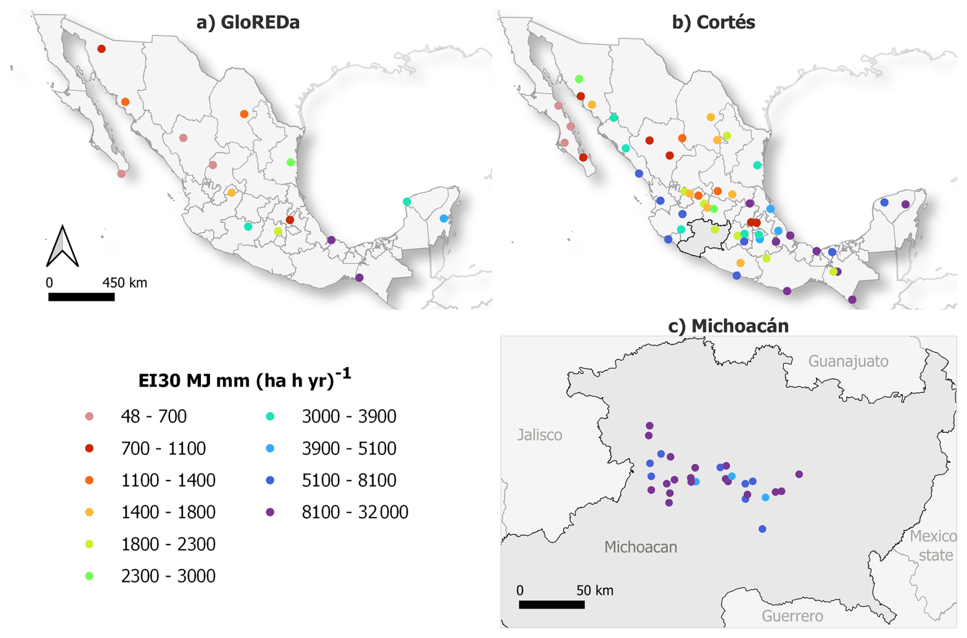
Figure 3Spatial distribution of the validation datasets: (a) GloREDa (n=15), (b) Cortés (n=44), and (c) Michoacán (n=23).
2.2.3 Comparison of the empirical relationships
We compared the three EI30 databases against the R factor estimates by using the three coefficients (α and β) combinations called Model I, Model II, and Model III. We identified the direct comparison against the validation databases and our estimated Mexican databases (Mexico-CN1, Mexico-CN2, and Mexico-CN3) according to the overlapping between periods. Thus, the GloREDa database was compared against the R factor calculated by using Mexico-CN3 (1988–2017). The Cortés database was compared against Mexico-CN1 (1968–1997) and Mexico-CN2 (1978–2007). The Michoacán database was compared against Mexico-CN3 (1988-2017). Afterwards, for each point in the GloREDa and Cortés databases, we identified the nearest point in the Mexican database produced in this study. Moreover, as the Michoacán database is a 15 min temporal resolution, we aggregated these rainfall time series at a daily resolution to estimate the R factor with the three coefficient combinations.
For those points in the Mexican databases, we calculated the daily erosivity Rd factor by using Model I, Model II, and Model III. Following, we calculated the annual erosivity Ry (MJ mm ha−1 h−1 yr−1) as the sum of the daily erosivity values in a year . Finally, the R factor corresponds to the mean annual rainfall erosivity values for a multi-year period .
We performed a linear regression to identify the relationship between the EI30 and R factor values. In this sense, the slope of the linear model quantifies the mean change in the R factor associated with a one-unit increase in EI30. Additionally, for each empirical model and validation database, we calculated the Mean Error (ME) and the Root Mean Square Error (RMSE) to evaluate the magnitude and direction of the differences between the estimated R factors and the observed EI30 values.
2.3 Rainfall erosivity estimation
We estimated the R factor for each weather station on the Mexican rainfall time series database. First, we identified the days with erosive rainfall as those with cumulative precipitation greater than 12.7 mm, an extension of the suggestion by Wischmeier and Smith (1978), Shin et al. (2019) and Efthimiou (2018). Second, we calculated daily erosivity Rd using the best coefficient combination identified in the previous step (Sect. 2.2). Finally, we estimated the mean annual rainfall erosivity, R factor, as described in the previous step (Sect. 2.2.3).
At this point, it is essential to highlight that we did not consider the erosivity due to the snowmelt because there is a pint-sized area covered with snow (or risk of snowfall), and no monitoring system for snowfall is publicly available in Mexico. To estimate the surface covered by snow, we explored the climate classification developed by García (1998), a modified Köppen classification system to better fit Mexico's climate conditions. According to the Köppen classification, only 83 km2 (0.004 % of the total area of Mexico) can be classified as E climates in the format of ET (tundra: temperature of warmest month greater than 0 °C but less than 10 °C) and EF (snow/ice: temperature of the warmest month 0 °C or below), both only produced by high altitudes. Additionally, the National Center for Disaster Prevention of Mexico developed a national snowfall danger index at a municipality level based on the occurrence of snowfall during the centuries XV to XXI (Jiménez Espinosa et al., 2012). They found that in the study period, snowfall had never occurred in 93.8 % of Mexico's municipalities. Additionally, the municipality with the highest snowfall frequency is Juarez (Chihuahua state), with just 30 events over five centuries.
Finally, to provide an overview of the sensitivity associated with the gap-filling and homogenization procedures, the complete rainfall time series were modified according to the percentage change in the mean value of each rainfall time series before and after these procedures. As established in the quality control section (Sect. 2.1.3), the mean change in the rainfall time series did not exceed 10 %. The modified series were subsequently used to recalculate daily rainfall erosivity values, from which new R factors were estimated for each station and climate normal. The percentage change between the recalculated R factor and the R factor estimated from the complete rainfall time series after the gap-filling and homogenization procedures was then computed to evaluate the sensitivity of rainfall erosivity estimates to alterations introduced during these procedures. This analysis provides a first-order assessment of the propagation of uncertainties associated with modifications in the rainfall time series into long-term erosivity estimates.
At the end of this step, we obtained three datasets with R factor values for the three CNs: Mexico-CN1 (1968–1997), Mexico-CN2 (1978–2007), and Mexico-CN3 (1988–2017).
This section presents the results of the three principal methodological stages outlined in the workflow. First, we developed a daily-resolution rainfall time series database, which provided a basis for further analysis. Second, we identified the best empirical relationship to estimate daily erosivity. Third, based on the best empirical relationship, we estimated rainfall erosivity values using the daily-resolution rainfall time series resulting from the first step.
3.1 Rainfall time series database development
The initial number of rainfall time series for the gap-filling, homogenization and quality control process was 1479; 1774; and 1721 for CN1, CN2, and CN3, respectively (Table 1). After data gap-filling, homogenization, and quality control, we discarded 4.8 % of the rainfall time series. Hence, Table 1 shows that the largest number of rainfall time series corresponds to CN1 (1968–1997), with 7.4 % (110 rainfall time series), which is followed by CN2 (1978–2007), with 5.4 % (96 rainfall time series), and CN3 (1988–2017), with 2.6 % (45 rainfall time series). Likewise, the most significant proportion of discarded rainfall time series corresponded to Mediterranean California (3 rainfall time series, 21.4 %) and North American Deserts (29 rainfall time series, 15.84 %) in CN1; Mediterranean California (2 rainfall time series, 11.11 %) and Great Plains (7 rainfall time series, 12.72 %) in CN2; and Great Plains (5 rainfall time series, 10.86 %) in CN3. Additionally, in the data gap-filling processes, we identified that none of the 5 rainfall time series available for Mediterranean California, in CN3, had a rainfall records for three consecutive years, which did not allow us to carry out the data gap-filling process for the complete study period; however, CN1 and CN2 provide a robust basis for assessing rainfall erosivity in this ecoregion. Finally, we obtained a database with 1369; 1678; and 1676 rainfall time series for CN1, CN2, and CN3, respectively. The available rainfall time series are distributed across the Mexican territory for the three CNs and represent the seven ecoregions (Fig. 4).
Table 1Number of available rainfall time series before and after data gap-filling process, as well as the number of discarded rainfall time series. The frequency of the rainfall time series is shown by ecoregion and climate normal.
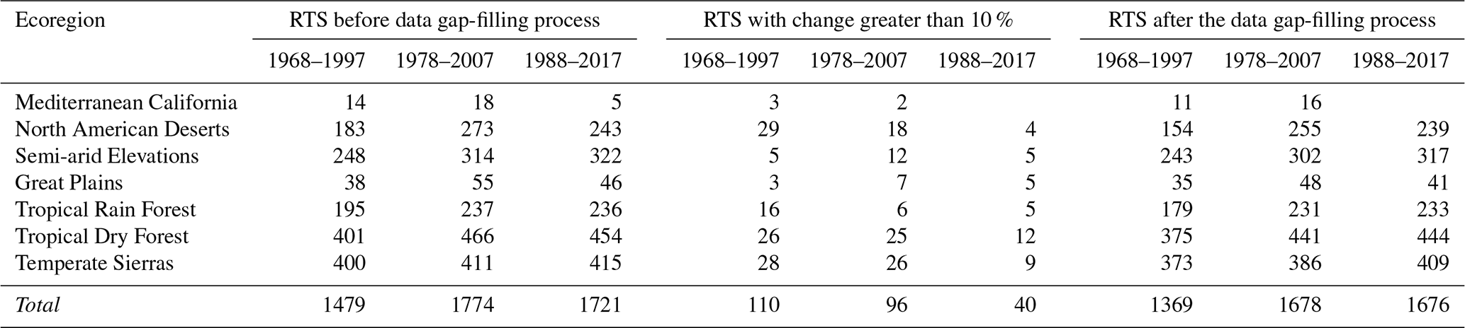
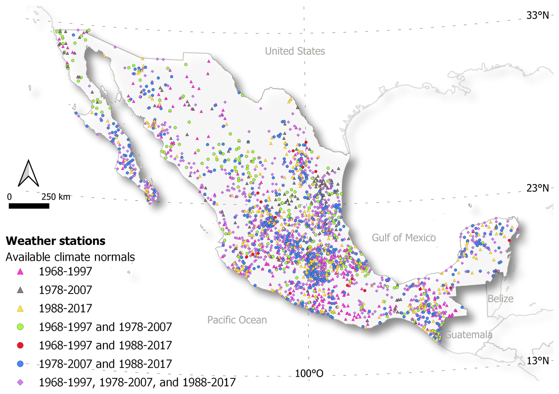
Figure 4Spatial distribution of the available weather stations for each climate normal: CN1 (1968–1997), CN2 (1978–2007), and CN3 (1988–2017).
The percentage of variation in the mean of the rainfall time series by ecoregion and CN using the two-step clustering is shown in Table 2. The CN2 (1978–2007) showed the highest average change in the mean, with −1.80 %, where it is also noted that four of the seven ecoregions present relatively high average changes. Notably, in CN1 (1968–1997), for North American Deserts, the highest average change in the mean is −1.50 %. In the CN3 (1988–2017), for Tropical Dry Forest and for Temperate Sierras, it is −3.38 % and −1.61 %, respectively. Additionally, Table A4 shows the Root Mean Square Error (mm) of the monthly accumulated rainfall by ecoregion. It can be seen that the highest RMSE was found for Tropical Rain Forest in the three CNs (6.12, 5.72, 6.78 mm, respectively), followed by Great Plains in CN2 and CN3 (5.72, 6.78 mm, respectively).
Table 2Mean percentage change in the mean value of rainfall time series by ecoregion.
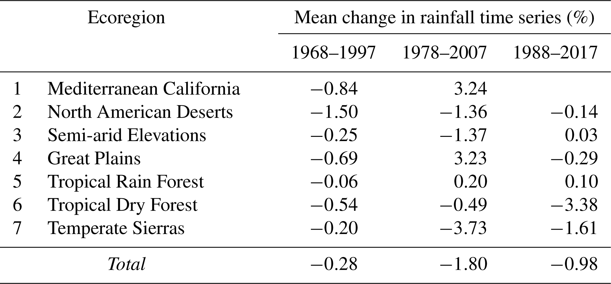
Figure A2 shows the monthly rainfall distribution for the seven ecoregions for CN1 (1968–1997), CN2 (1978–2007), and CN3 (1988–2017). The results indicate that Mexico exhibits a unimodal rainfall regime, with a marked peak and a well-defined dry season across all ecoregions; however, the characteristics of the wet period vary among them. In the Tropical Rain Forest, rainfall increases rapidly from May to June and peaks in September, with monthly values exceeding 300 mm. The Tropical Dry Forest and the Temperate Sierras show a similar annual pattern, with a persistent and evenly distributed wet season from June to September, reaching monthly values of around 200 mm. In the Semi-arid Elevations, the wet period begins in May, peaks in July (approximately 150 mm), and declines gradually until October. The Great Plains ecoregion exhibits a wet season that begins in March, followed by a gradual increase in rainfall, sustained precipitation through July (around 100 mm), and a peak in September (approximately 150 mm). In contrast, the North American Deserts ecoregion is characterised by low rainfall throughout the year, with only a modest increase during the summer months (around 50 mm), and no clear peak. The Mediterranean California ecoregion shows a markedly different pattern, with rainfall concentrated between November and March, reaching monthly values of approximately 50 mm. Overall, the general behavior of rainfall distribution across ecoregions is consistent among the three climate normals. However, slight differences are observed in CN3, where the North American Deserts show an increase in accumulated precipitation in September, and the Great Plains show an increase in July precipitation.
3.2 Identification of the best empirical relationships to estimate erosivity in Mexico
This section presents the results of identifying the best empirical relationship between EI30 and the R factor calculated from three models. To achieve this, we built linear models to identify the rate of change between the EI30 factor and the R factor estimated with the three models (Fig. 5). In this context, a slope of 1 indicates perfect agreement between estimated R factors and EI30 values, whereas deviations from 1:1 slope reflect fewer agreement.
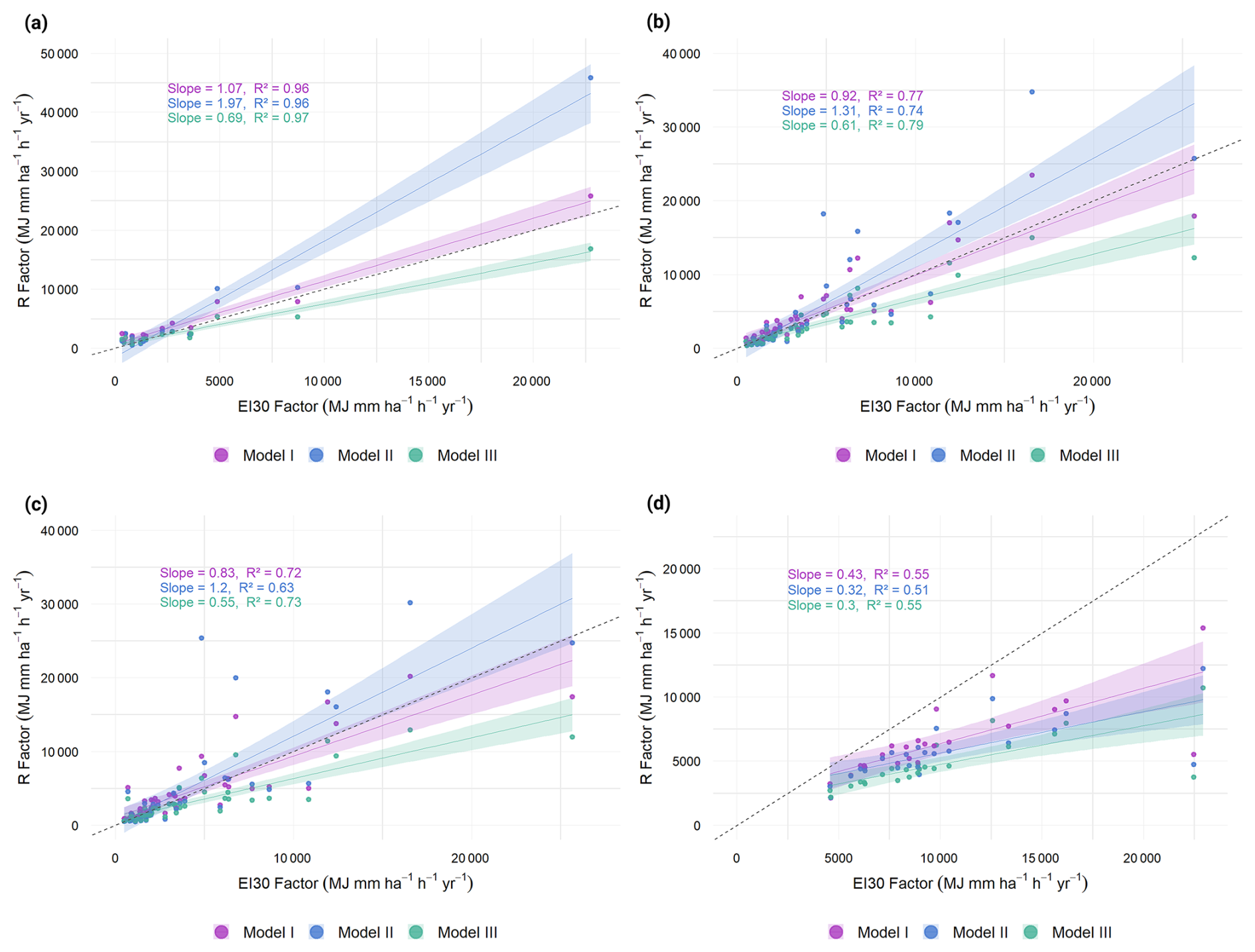
Figure 5Comparison between observed EI30 factor and rainfall erosivity estimates (R) factor obtained using the three evaluated models across different datasets: (a) global (GloREDa), (b) national (Cortés; Mexico-CN1), (c) national (Cortés; Mexico-CN2), and (d) local (Michoacán). The x-axis represents observed EI30 values, while the y axis shows model-based rainfall erosivity estimates derived from daily rainfall time series. Solid lines indicate the fitted linear regression for each model, and the dashed line represents the 1:1 relationship (perfect agreement). The slope of each regression is used as an indicator of model performance.
Table 3Metrics of performance of three models: Model I (Richardson et al., 1983), Model II (Liu et al., 2020), and Model III (Xie et al., 2016) in predicting the EI30 values of three databases: GloREDa, Cortés and Michoacán. ME: Mean error and RMSE: Root Mean Square Error.
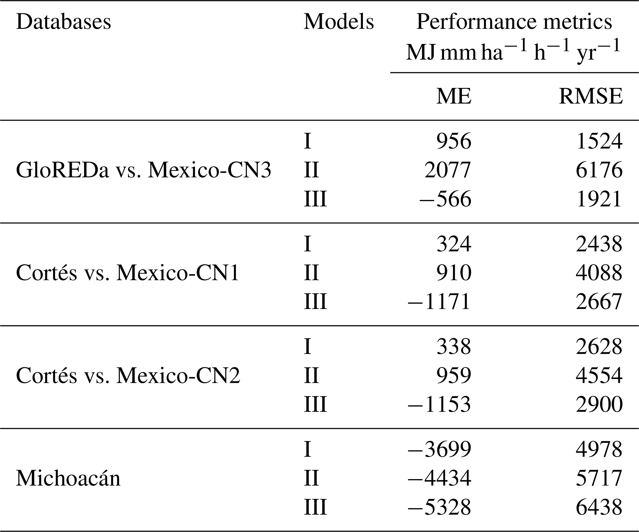
Model I was the coefficient combination with the best overall performance across the three datasets, with slopes closest to 1 (1.07, 0.92, 0.83, and 0.43 for GloREDa vs. Mexico-CN3, Cortés vs. Mexico-CN1, Cortés vs. México-CN2 and for the Michoacán database, respectively) and the lower RMSE values (1524; 2438; 2628; and 4978 MJ mm ha−1 h−1 yr−1 for GloREDa vs. Mexico-CN3, Cortés vs. Mexico-CN1, Cortés vs. México-CN2 and for the Michoacán database, respectively). Whereas, Model II obtained the poorest performance for GloREDa vs. Mexico-CN3, Cortés vs. Mexico-CN1, and Cortés vs. México-CN2 with the highest RMSE values (6176; 4088; and 4554 MJ mm ha−1 h−1 yr−1, respectively). Model III showed intermediate RMSE values, but consistently underestimated EI30 values in all datasets (negative ME values). For the Michoacán dataset, all three models underestimated EI30, with Model I still providing the best performance (ME = −3699; RMSE = 4978 MJ mm ha−1 h−1 yr−1), followed by Models II and III, which showed progressively larger errors.
On the other hand, the distance of each point of the GloREDa and Cortés (Mexico-CN1 and Mexico-CN2) database to the nearest weather station varied in a range of 0.6 to 42.0 km (mean: 11.6 km), 0.3 to 73.4 km (mean: 12.17 km), and 0.3 to 76.5 km (mean: 10.7), respectively. It is important to highlight that there is no correlation between error and the distances between points in the validation datasets and the weather stations of our Mexican database.
3.3 Rainfall erosivity estimates
In this section, we present the results of rainfall erosivity estimates for the three climate normals considered. First, we describe the statistical distribution of erosivity values, followed by their annual distribution and, finally, their spatial distribution.
Figure A3 shows the mean number of locations with erosive rainfall for each day of the year for the three climate normals. In all CNs, erosive rainfall is concentrated within a single annual erosive season extending approximately from days 150 to 280, corresponding to the summer rainfall period in Mexico. For CN1, the erosive period is relatively stable, with the highest number of locations with erosive rainfall occurring between days 170 and 260. Similarly, CN2 exhibits a well-defined erosive season, although with slightly greater variability and higher peaks than CN1. In contrast, CN3 is characterised by a more pronounced intra-seasonal variability, with two distinct peaks occurring between days 173–190 and 229–261. These peaks correspond to periods when the number of locations reporting erosive rainfall exceeds the 90th percentile. Additionally, the 90th percentile threshold of the number of locations with erosive rainfall increases from 211 in CN1 to 227 in CN2 and 238 in CN3, representing increases of 7 % and 12 %, respectively, relative to CN1.
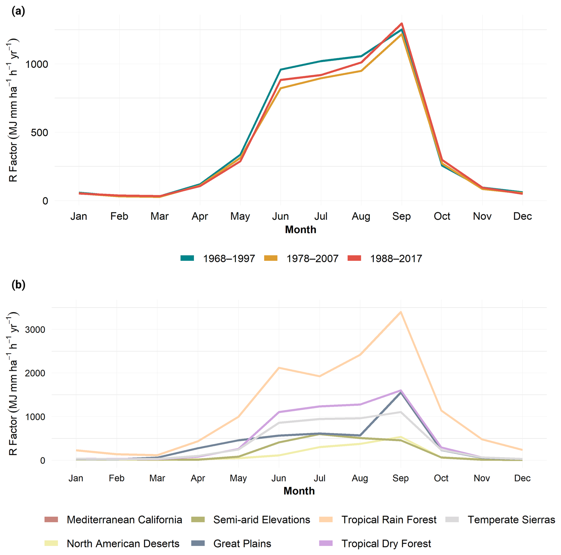
Figure 6Monthly erosivity values estimated from daily rainfall time series and using the Richardson et al. (1983) power-law model. (a) Monthly erosivity for the three climate normals; (b) monthly erosivity by ecoregion for the Mexico-CN3 (1988–2017).
The mean values of rainfall erosivity for CN1, CN2, and CN3 were 5276 (SD 5662) MJ mm ha−1 h−1 yr−1, 4832 (SD 5266) MJ mm ha−1 h−1 yr−1, and 5067 (SD 5071) MJ mm ha−1 h−1 yr−1, respectively (Table 4). The statistical distribution of the rainfall erosivity values was right-skewed with skewness of 2.7, 3.0, and 2.9 for CN1, CN2, and CN3, respectively. So the median was less than the mean with values of 3245; 3070; and 3327 MJ mm ha−1 h−1 yr−1 for CN1, CN2, and CN3, respectively. The Krustal–Wallis test showed that the erosivity median value for CN2 differed from CN1 and CN3 at a 95 % confidence level. The kurtosis values of 12.6, 15.1, and 15.3 for CN1, CN2, and CN3, respectively, indicate large tails with the presence of outliers. In this case, the outliers are high erosivity values reaching more than 12 000 MJ mm ha−1 h−1 yr−1 for the three CNs (Fig. A4).
Table 4Descriptive statistics of the erosivity values for three climate normals (1968–1997, 1978–2007, 1988–2017). Min: minimum, Max:maximum, SD: standard deviation, CV: coefficient of variation, skew: skewness, kurt: kurtosis.

Monthly erosivity varies throughout the year in the three CNs (Fig. 6a). The behavior of the erosivity in the three CNs is monomodal, indicating just one peak and one valley. The month with the highest erosivity is September, reaching values almost to 1300 MJ mm ha−1 h−1 yr−1, followed by August, July, and June with erosivity values around 1000 MJ mm ha−1 h−1 yr−1. It is important to highlight that for June, July, and August, the CN1 (1968–1997) had the highest monthly erosivity values; however, for September, the highest values are found in the CN2 (1988–2017). The months with the smallest erosivity values are February, followed by March with values less than 40 MJ mm ha−1 h−1 yr−1.
As the three CNs had the same behavior throughout the year, we displayed in Fig. 6b the monthly erosivity for CN3 by ecoregion. The Tropical Rain Forest exhibits the highest erosivity values throughout the year, ranging from a minimum in March (114 MJ mm ha−1 h−1 yr−1) to a maximum in September (3395 MJ mm ha−1 h−1 yr−1). In contrast, the North American Deserts show the lowest erosivity values, generally remaining below 500 MJ mm ha−1 h−1 yr−1. Most ecoregions reach their maximum erosivity in September; however, the Semi-arid Elevations peak earlier, in July. It is important to note that CN3 does not include stations in the Mediterranean California ecoregion. Nevertheless, in CN1 and CN2, this ecoregion shows the lowest erosivity values among all regions.
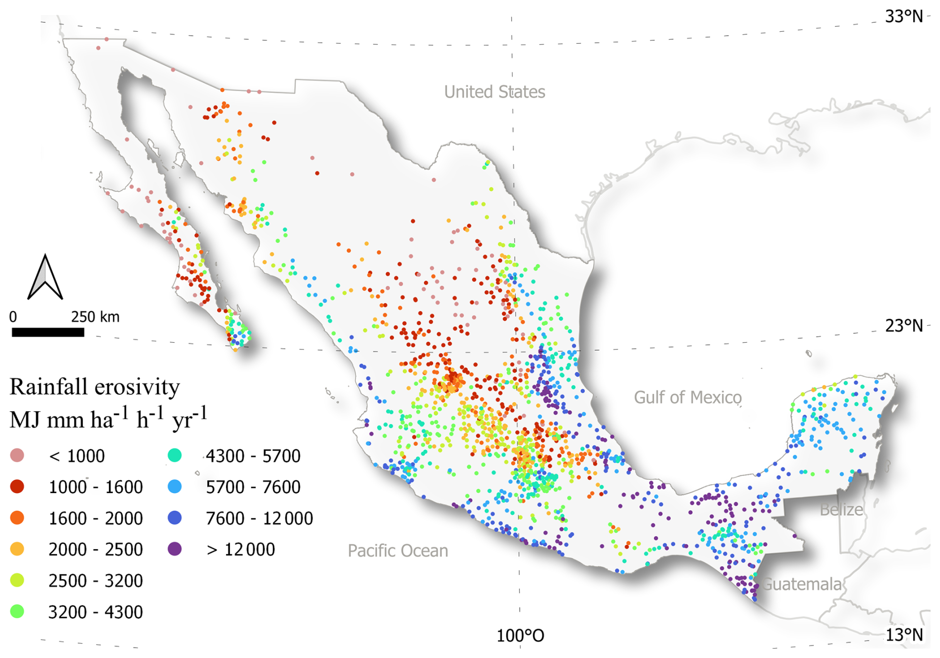
Figure 7R factor values calculated with the power law equation proposed by Richardson et al. (1983) at daily resolution for the climate normal 1988–2017. The legend classes approximately represent deciles of the statistical distribution, although not exactly.
Regarding the spatial distribution, the erosivity values across Mexican territory look similar for the three CNs (Figs. 7 and A5). Low erosivity values (<1000 MJ mm ha−1 h−1 yr−1) are mainly concentrated in the Baja California peninsula and northern Mexico, corresponding to arid regions such as the North American Deserts and Semi-arid Elevations. Intermediate values (approximately 1600–4300 MJ mm ha−1 h−1 yr−1) are distributed across central Mexico, reflecting transitional climatic conditions. In contrast, the highest erosivity values (>7600 MJ mm ha−1 h−1 yr−1) are concentrated in the southern and southeastern regions of the country. These areas correspond to the upper deciles of the statistical distribution, indicating a strong spatial concentration of high erosive potential in humid tropical environments. This spatial pattern is also reflected in the mean erosivity values calculated for each ecoregion (Table A5). The Tropical Rain Forest consistently exhibited the highest mean erosivity values for the three climate normals, followed by the Tropical Dry Forest, Temperate Sierras, and Great Plains. In contrast, the Mediterranean California and North American Deserts ecoregions showed the lowest mean erosivity values. Across the three climate normals, the relative hierarchy among ecoregions remained similar, with tropical and humid regions presenting substantially higher erosivity values than arid and semi-arid regions.
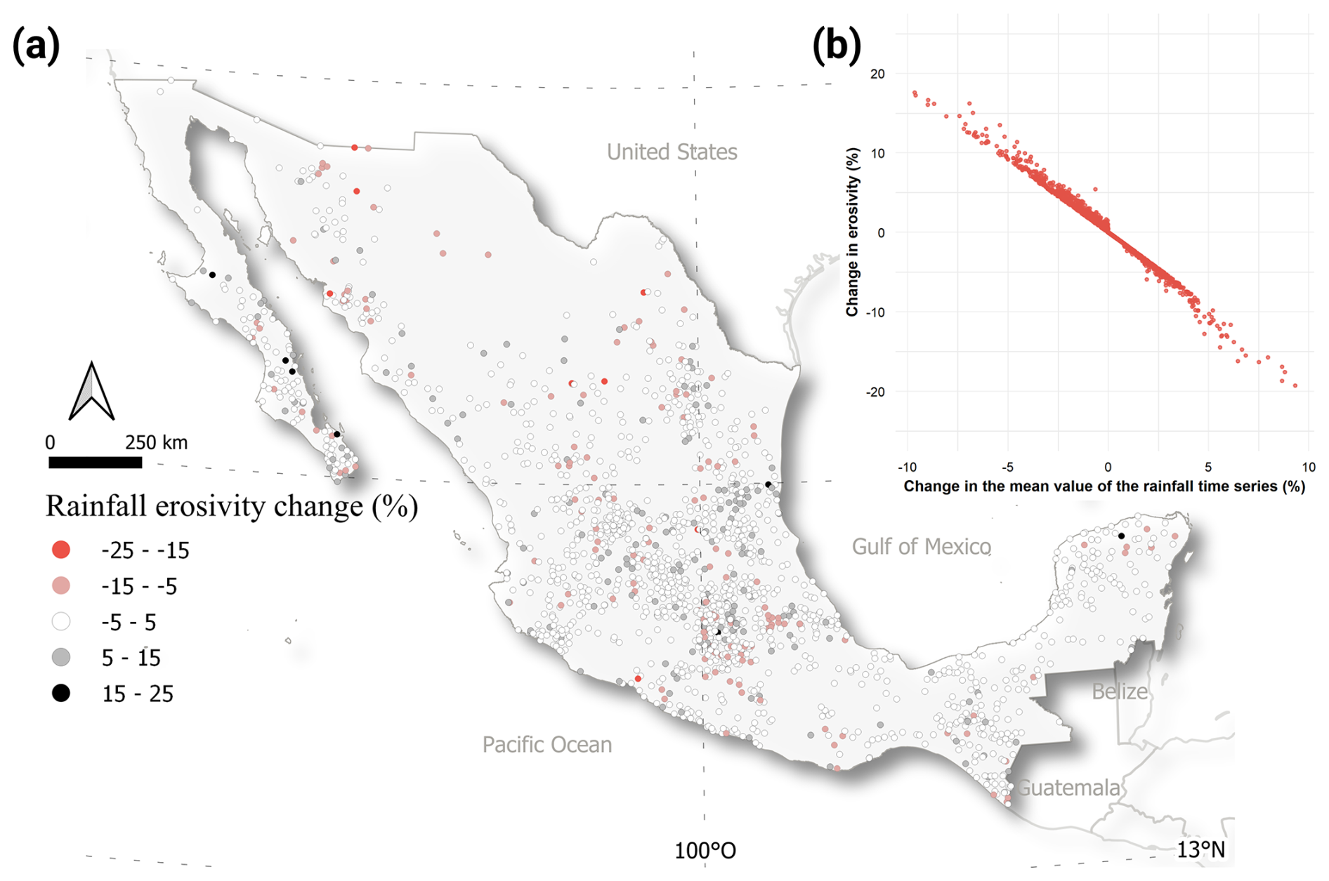
Figure 8Percentage changes in rainfall erosivity after modifying precipitation time series according to the percentage change in the mean value of the rainfall time series before and after the gap-filling and homogenization processes for the 1988–2017 climate normal. (a) Spatial distribution of percentage changes in rainfall erosivity. (b) Relationship between percentage changes in the mean value of the rainfall time series and percentage changes in rainfall erosivity.
The spatial distribution of percentage changes in rainfall erosivity after the homogenization and gap-filling procedures was heterogeneous across the three climate normals, with positive and negative changes interspersed throughout Mexico (Fig. 8a for the CN3 and Fig. A6a for the CN1 and CN2). In all climate normals, most stations exhibited relatively small changes, generally between −5 % and 5 %. CN1 showed a slight predominance of positive changes in northern Mexico, particularly in the Baja California Peninsula and northwestern regions, whereas CN2 displayed a more balanced distribution of positive and negative changes across the country. In contrast, CN3 exhibited a greater occurrence of negative changes in northern and northwestern Mexico. Southern Mexico and the Yucatán Peninsula generally showed lower magnitudes of change across the three climate normals. Overall, the largest positive and negative changes were associated with isolated stations rather than coherent regional clusters.
The scatterplots reveal a consistent inverse relationship between the percentage change in the mean rainfall series after the homogenization and gap-filling procedures and the corresponding percentage change in rainfall erosivity across the three climate normals (Fig. 8b for the CN3 and Fig. A6b for the CN1 and CN2). The three climate normals exhibited a similar funnel-shaped distribution, in which the dispersion of erosivity changes increased progressively as the magnitude of rainfall change became larger. Stations with precipitation changes close to 0 % showed relatively small erosivity variations concentrated near zero, whereas stations with larger positive or negative rainfall changes exhibited a wider range of erosivity responses, reaching approximately ±20 %.
Table A5 summarizes the percentage changes in rainfall erosivity by ecoregion for the three climate normals after the homogenization and gap-filling procedures. Overall, mean percentage changes remained low across all ecoregions and climate normals, with most values below 3 %. For CN1, the largest mean positive percentage changes were observed in the North American Deserts (2.3 %) and Mediterranean California (2.1 %). In CN2, mean percentage changes were generally smaller, although the North American Deserts still exhibited the largest positive mean change (1.7 %), while the Great Plains showed a slight negative mean change (−0.6 %). Similarly, in CN3, mean percentage changes remained close to zero across ecoregions, ranging from −0.4 % in the North American Deserts and Great Plains to 0.7 % in the Tropical Dry Forest. Although the mean changes were comparatively small at the ecoregional scale, some individual stations exhibited larger positive and negative percentage changes. The maximum positive changes reached 21.2 %, 19.3 %, and 17.6 % for CN1, CN2, and CN3, respectively, whereas the minimum changes reached −18.8 %, −23.0 %, and −19.3 %. Overall, the range of percentage changes was similar among the three climate normals, with both positive and negative changes occurring within comparable magnitudes.
This research addressed the data incompleteness and breakpoints in the legacy Mexican climate time series. Particularly, we compiled and systematized a national dataset with daily rainfall and rainfall erosivity for three climate normals (CN1: 1968–1997, CN2: 1978–2007, and CN3: 1988–2017) across Mexico. To the best of our knowledge, this research is the first effort to develop a large daily rainfall time-series and erosivity dataset at the national scale, based on legacy climate data, following the quality-control and inhomogeneity analyses proposed by the World Meteorological Organization. This discussion is organized into four principal components. First, we discuss the development and quality-control procedures of the first national rainfall time series database for Mexico, including the implications of homogenization across contrasting climatic regions. Second, we analyse the rainfall erosivity estimates, their spatial patterns, and the performance of the empirical models used for daily erosivity estimation. Third, we evaluate the sensitivity of rainfall erosivity estimates to the homogenization and gap-filling procedures. Finally, we discuss the limitations, potential applications, and future research directions associated with the rainfall and erosivity databases
4.1 Development of the first Mexican rainfall time series database
-
Improvement over the previous rainfall products in Mexico: Previous national-scale rainfall datasets for Mexico are those produced by Cuervo-Robayo et al. (2014) and Carrera-Hernández (2025); they emphasise spatial completeness through interpolation. (Cuervo-Robayo et al., 2014) updated the mean monthly rainfall for 100 years (1910–2009) using around 5000 rainfall time series and used thin-plate smoothing spline interpolation to generate gridded data at 30 arcsec spatial resolution for the continental area of Mexico. Similarly, Carrera-Hernández (2025) developed the Mexico High Resolution Climate Database (MexHiResClimDB), a gridded dataset that provides daily, monthly, and annual rainfall for the period 1951–2020, using up to 4000 rainfall records per day. This dataset was generated using kriging with external drift on a local neighbourhood, producing gridded data at 20 arcsec spatial resolution across Mexico.
These approaches prioritize spatial completeness and provide valuable insights into the spatial distribution of climate variables across Mexico. However, previous gridded datasets either did not perform quality control (Cuervo-Robayo et al., 2014) or applied only basic quality control procedures (Carrera-Hernández, 2025), such as selecting stations with more than 80 % of recorded data for at least 10 consecutive years and discarding unrealistic values (e.g., daily rainfall exceeding 600 mm). However, climatological studies have shown that inhomogeneities in rainfall time series can introduce biases and artificial trends, potentially leading to erroneous interpretations and misleading conclusions (Adeyeri et al., 2017). In consequence, WMO (2017, 2023) guidelines recommend that rainfall data undergo a comprehensive set of quality control tests, including constraint, consistency, rapid change, and domain analysis. These procedures are essential to ensure the reliability of climatic analyses, avoid biases due to measurement or recording errors, and maintain comparability across stations and regions, particularly in long-term rainfall time series.
Therefore, although gridded datasets are important for understanding large-scale ecological processes across Mexico, generating climate data from reliable and quality-controlled time series is equally important. This represents a key strength of our rainfall dataset compared to previous efforts. By providing a robust and quality-controlled rainfall time series database, we ensure greater reliability for climate analyses that depend on the accurate representation of extreme events and temporal variability, including rainfall erosivity estimation, hydrological modeling, and climate extremes assessment.
-
Changes in the mean monthly rainfall by ecoregion: since the homogenization process corrects outliers, artificial breaks, and inconsistencies in the raw records, larger RMSE values may reflect stronger corrections applied to low-quality or highly inhomogeneous rainfall series (Adeyeri et al., 2022). In this sense, the RMSE partly reflects the initial quality of the raw rainfall time series rather than solely the uncertainty introduced during the reconstruction process. Consequently, the RMSE also provides insight into the importance of homogenization and quality-control procedures across ecoregions, where breakpoints and outliers may affect rainfall series differently depending on the climatic regime. For example, in the Tropical Rain Forest ecoregion, the RMSE value for October was 12.11 mm, whereas the corresponding mean monthly precipitation was 230.9 mm, representing a relative deviation of only 5.4 % with respect to the raw series. In contrast, in the North American Deserts, the RMSE value for March was only 2.08 mm; however, because the corresponding mean monthly precipitation was 7.97 mm, this represented a relative deviation of 26 %. These comparisons indicate that rainfall series without homogenization may produce proportionally larger distortions in climatic variability and long-term trend analyses in arid and semi-arid regions, where low rainfall magnitudes amplify the effect of outliers and artificial breaks. This is particularly relevant because arid and semi-arid regions represent approximately 41.7 % of the continental area of Mexico.
-
Rainfall patterns across Mexico: the rainfall patterns observed across ecoregions are clearly influenced by both global climate dynamics and local topographic conditions. Overall, Mexico exhibits a unimodal rainfall regime, with a wet period occurring during late spring and summer (May to October), as reported by Carrera-Hernández (2025). However, the characteristics of this rainfall regime vary among ecoregions. For example, in the Tropical Dry Forest and Temperate Sierras (principally located over the Sierra Madre Occidental and the Eje Neovolcánico), the rainy season is concentrated between July and September. This pattern is largely driven by the North American Monsoon, which develops from July to September and originates along the western coast of Mexico (Gochis et al., 2006). During this period, a pressure gradient draws warm, moist air inland from the Pacific Ocean and the Gulf of California, and winds transport this moisture toward the interior. As the air rises over the Sierra Madre Occidental, it cools and condenses, producing convective rainfall, typically in the afternoon (Boos and Pascale, 2021). In addition to the monsoonal influence, the Tropical Rain Forest (located mainly in southeastern Mexico) exhibits a rainfall pattern associated with the northward migration of the Intertropical Convergence Zone, enhanced convective activity, and the contribution of tropical cyclones during late summer (August and September), resulting in increased monthly precipitation (de Anda Sánchez, 2020).
In contrast to the tropical and monsoonal processes that dominate rainfall across most of Mexico, the Mediterranean California rainfall pattern is influenced by different climate dynamics. This ecoregion is located in the northwesternmost part of Mexico (Fig. 1) and is characterised by hot, dry summers and wet winters (García, 1998). Winter rainfall is associated with frontal storms originating in the Pacific Ocean (Deitch et al., 2017), linked to the position of the region on the equatorward flank of mid-latitude storm tracks and the poleward edge of the Hadley cell. In contrast, dry summer conditions are related to descending air and atmospheric subsidence associated with the eastern flanks of subtropical anticyclones (Seager et al., 2019).
4.2 Rainfall erosivity estimates and model performance
-
Evaluation of empirical models for daily erosivity estimation: among the three coefficient combinations evaluated for estimating daily rainfall erosivity, the Richardson et al. (1983) proposal consistently demonstrated superior performance across the national and local datasets. Although all three models adopt a similar functional structure of the form R=αPβ, differences in the parameterisation of the α and β coefficients have substantial implications for model behavior under diverse rainfall regimes. The Richardson et al. (1983) equation was developed using rainfall time series across the United States of America, including rainfall conditions of the southern states such as Georgia, Mississippi, and Texas. This equation defines different α coefficients for the cool and warm seasons that occur from October to March and from April to September, respectively; it is very similar for the Mexican climate, where it is seen that the warmest months are those from May to October (Carrera-Hernández, 2025). Additionally, the β coefficient has no spatial or seasonal pattern, the same as found in the Xie et al. (2016) equation and contrary to the Liu et al. (2020) one, where the β coefficient is affected by the latitude in the Tropical (A) climate classification according to Köppen–Geiger. However, it is notable that the β coefficient for Richardson et al. (1983) equation (1.81) is slightly higher than that for Xie et al. (2016) and Liu et al. (2020) (1.72 and between 1.5 and 2 depending on the latitude, respectively), placing greater weight on high rainfall amounts which may better capture the erosive potential of intense storms. Indeed, this is the reason why the Richardson et al. (1983) model obtained the highest erosivity estimates for the Michoacán dataset (purple points always over the blue and green dots in Fig. 5d), because β coefficients for all the Michoacán dataset were 1.81, 1.558 and 1.72 for the three models Richardson et al. (1983), Liu et al. (2020), and Xie et al. (2016), respectively.
-
Erosivity estimates: our work reveals that the distribution of erosivity values in Mexico corresponds to the geographical distribution of rainfall and seasonal precipitation conditions. The areas with the highest erosivity values are concentrated in the Isthmus of Tehuantepec (i.e., the shortest distance between the Gulf of Mexico and the Pacific Ocean). This region corresponds to the Tropical Rain Forest ecoregion, where high moisture availability enhances extreme precipitation events, increasing rainfall erosivity (Wang et al., 2023b). High values are also concentrated along the Pacific coastal zone and in low-elevation areas of the Sierra Madre Occidental, where previous studies have reported intense precipitation events at hourly and daily timescales (Gochis et al., 2006). In contrast, lower erosivity values occur in the central and northern regions of Mexico, where severe droughts (e.g., those occurring from the 1990s to the beginning of the twenty-first century), associated with large-scale ocean–atmosphere circulation patterns, have reduced mean annual rainfall. We also highlight a hotspot in the southern part of the Baja California Peninsula (e.g., Sierra La Laguna), where erosivity values are higher than those estimated for the northern part of the peninsula. This local variation is associated with the influence of tropical cyclones, which contribute up to 50 % of the mean annual rainfall in this region (Agustín Breña-Naranjo et al., 2015). Overall, the spatial variability of erosivity across Mexico reflects the interplay between rainfall regimes and climatic events, underscoring the strong influence of regional atmospheric processes on soil erosion dynamics.
In agreement with these spatial patterns, our rainfall erosivity estimates are generally higher than those reported for Mexico by global products such as GloRESatE (Das et al., 2024) and GloREDa (Panagos et al., 2017). The GloRESatE grid reports erosivity values ranging from 49 to 49 811 MJ mm ha−1 h−1 yr−1, with the highest values located in southern Chiapas. Similarly, the GloREDa grid reports values between 51 and 13 058 MJ mm ha−1 h−1 yr−1, identifying the highest erosivity in the Isthmus of Tehuantepec and the coastal zone of the Gulf of Mexico. In contrast, our database reports maximum erosivity values exceeding 43 000 MJ mm ha−1 h−1 yr−1 in the tropical regions of southern Mexico. Additionally, Tong et al. (2026) reported erosivity values ranging from 8000 to 20 000 MJ mm ha−1 h−1 yr−1 for the Yucatán Peninsula, further supporting the occurrence of high erosivity conditions in tropical regions of Mexico.
Despite differences in magnitude, both global products and our dataset consistently identify tropical regions as the areas with the highest erosivity. This pattern is also consistent with the global distribution of EI30 values reported in the databases used to construct these products. For example, the GloRESatE database (Das et al., 2024), which contains approximately 6,200 sites worldwide, reports a maximum EI30 value of 39 124 MJ mm ha−1 h−1 yr−1 in Bangladesh. Likewise, the GloREDa database (Panagos et al., 2017), based on 3940 sites globally, reports a maximum erosivity value of 58 288 MJ mm ha−1 h−1 yr−1 in Las Cruces, Costa Rica. These comparisons suggest that the high erosivity values observed in tropical regions of southern Mexico are consistent with the global tendency for extreme erosivity to occur in humid tropical environments.
Conversely, the lowest erosivity values in our database are associated with the arid regions of northern Mexico and are consistent with those reported by GloREDa and GloRESatE. Although there are no specific EI30 estimates available for these Mexican arid regions, comparable values have been reported for the southern United States, which shares similar climatic conditions. For example, Kim et al. (2020) estimated EI30 values between 500 and 1000 MJ mm ha−1 h−1 yr−1 using CMORPH satellite data with a temporal resolution of 30 minutes and a spatial resolution of 8 km. Similarly, the GloRESatE database (Das et al., 2024), which includes a large number of weather stations across the United States, reports erosivity values ranging from 400 to 1200 MJ mm ha−1 h−1 yr−1 near the Mexico–United States border. These comparisons indicate that the low erosivity values identified in northern Mexico are consistent with the broader climatic conditions of arid and semi-arid regions in North America.
-
Improvement over previous erosivity datasets: this new erosivity dataset is appealing due to two principal advantages: spatial and temporal coverage. It provides erosivity values for a substantially larger number of sites (1369, 1678, and 1676 for CN1, CN2, and CN3, respectively) compared to the dataset developed by Panagos et al. (2023), which includes erosivity estimates for 15 sites in Mexico, and the dataset compiled by Cortés (1991), which estimated erosivity values for only 53 sites across the country. Additionally, this dataset improves the representation of rainfall erosivity conditions in several regions, particularly in the north of Mexico (e.g., Chihuahua and Baja California), the central region (e.g., Zacatecas and Querétaro), and the south (e.g., Campeche and Quintana Roo), where erosivity estimates were previously unavailable. Additionally, this database provides erosivity estimates for the most rainy regions in Mexico, such as the Pacific coast and the isthmus of Tehuantepec
On the other hand, this database is appealing for presenting multi-annual erosivity values for three climate normals covering the period from 1968 to 2017. As defined by Wischmeier and Smith (1978), estimating the R factor requires a long-term rainfall time series for reasonable estimates. Some studies have reported different minimum lengths required for a reliable estimation of rainfall erosivity: 5 years (Wang et al., 2024), 10 years (Verstraeten et al., 2006), 15 years (Hanel et al., 2016), and 20 years (Vantas et al., 2019; Renard and Freimund, 1994). In contrast, previous datasets have reported erosivity estimates from rainfall time series with a length between 1 and 11 years (Cortés, 1991) and 5 and 10 years in Panagos et al. (2023). This new database is appealing for the need of long-term rainfall time series to mitigate the seasonal and cyclical rainfall biases in the estimation of rainfall erosivity (Kumar et al., 2026).
-
Sensitivity of R factor estimates to homogenization and gap-filling process: to evaluate the implications of the homogenization and gap-filling procedures on rainfall erosivity estimates, we analyzed both the sensitivity of erosivity responses to changes in the rainfall time series and the spatial distribution of these changes across Mexico. The results reveal that homogenization may locally modify erosivity estimates; however, the spatial structure of rainfall erosivity patterns remains consistent across ecoregions. The funnel-shaped distribution observed in the scatterplots (Figs. 8b and A6b) indicates a high sensitivity in the erosivity estimates to the larger changes in the mean of the rainfall time series (Pianosi et al., 2016). This sensitivity is explained by the potential model implemented in erosivity estimation (Xie et al., 2016), but it could also partly be explained by changes in the number of erosive rainfall days. Since daily erosivity was calculated only for days exceeding the erosive rainfall threshold (12.7 mm), modifications introduced during homogenization and gap filling may cause some days to move above or below this threshold. As a result, changes in rainfall can affect both the magnitude of daily erosivity and the frequency of erosive days, leading to greater dispersion in erosivity responses as rainfall changes become larger.
The absence of spatially coherent clusters of positive or negative erosivity change suggests that the effects of the homogenization and gap-filling procedures were not primarily controlled by regional climate conditions. This is particularly relevant because the gap-filling process was performed within ecoregions, using neighbouring stations in the same climatic context (Adeyeri et al., 2022). Therefore, if the procedure had introduced a systematic regional bias, changes would be expected to appear spatially concentrated within specific ecoregions. Instead, the largest changes occurred at isolated stations, suggesting that they are more likely associated with the initial quality of individual non-homogenized rainfall time series. In this sense, larger percentage changes in the mean of the rainfall time series should be interpreted as indicators of stronger corrections applied to the raw rainfall time series, rather than as evidence of systematic distortion introduced by the homogenization process. Thus, the spatially scattered distribution of changes supports the interpretation that the homogenization procedure corrected station-specific inconsistencies while preserving the broader ecoregional rainfall structure.
4.3 Limitations and potential applications of the new databases
-
Limitations of the rainfall and erosivity databases: models based on coarser rainfall time series can underestimate and overestimate EI30 values, as observed in this study. Although calculated at a coarser temporal resolution, underestimations have already been indicated by Tu et al. (2023); Yin et al. (2015) while evaluating the effect of modifying the time interval for calculating EI30 using 5, 15, 30, and 60 min rainfall time series. The authors concluded that increasing the time interval leads to underestimating erosivity values. Similarly, Li et al. (2022) identifies that using a monthly model underestimates EI30. However, the same author found an overestimation of the R values regarding EI30 using annual models. However, no matter under or overestimation, it has been reported that when coarser time intervals are used instead of high temporal resolution, the relationship between E and I30 remains consistent, but a larger calibration coefficient is needed (Tu et al., 2023). Therefore, having more detailed information is arguably the best way to estimate the erosivity factor with greater certainty and to know which model explains the greatest variance of EI30.
In this study, the best-performing coefficient combination was that proposed by Richardson et al. (1983). However, we did not differentiate parameter coefficients by ecoregion due to the limited availability of sites with EI30 values. In regions with high-intensity rainfall events, such as the Pacific coastal zone of Mexico, rainfall tends to exhibit greater erosivity than in regions with lower-intensity rainfall, even when total rainfall amounts are similar. Under these conditions, coefficient parameters are expected to vary across regions (Li et al., 2022; Chen et al., 2020), reflecting differences in the erosive power of rainfall. Additionally, the choice of model and its associated coefficients constitutes an important source of uncertainty in subsequent soil loss estimation, which should be taken into account by users (Li et al., 2022).
-
Potential applications of the rainfall erosivity database: this new database will help as an indicator of rainfall erosivity patterns across Mexico. We report daily rainfall at a wide range of altitudes from 1 to 4283 m a.s.l. (above sea level). This is a valuable rainfall database because it is meeting the three primary requirements to the Universal Soil Loss Equation (USLE) and its derived models: (1) estimation of average annual rainfall erosivity for predicting long-term soil loss; (2) construction of seasonal erosivity curves to reflect the interaction between rainfall distribution and crop management practices; and (3) calculation of daily or 10-year return period erosivity values to assess the impact of extreme events on runoff generation and the effectiveness of soil conservation measures, such as terracing Yin et al. (2017).
In this context, this erosivity database represents a valuable tool for local, national, and global erosion studies. At the local scale, it can support the design of field experiments to validate rainfall erosivity estimates under different rainfall regimes, as well as the identification of the magnitude of underestimation or overestimation associated with different temporal resolutions of rainfall data (Meng et al., 2021; Zhao et al., 2019; Dunkerley, 2019). Finally, because this database spans a long period (1968–2017) and is divided into three climate normals, it enables users to analyse trends in rainfall and rainfall erosivity values and relate them to other erosion drivers, such as land use and soil cover dynamics (Yan et al., 2014).
At the national scale, this database can be used as input for erosion models to establish a baseline of soil loss rates across Mexico; indeed, the need for reliable erosivity values has been highlighted in previous studies (Bolaños González et al., 2016). Additionally, within the framework of the United Nations Convention to Combat Desertification, countries have the opportunity to report their contributions to the Sustainable Development Goals, including Indicator 15.3.1, which measures the proportion of degraded land relative to the total land area (Sims et al., 2021). In this context, Mexico could use this database to improve the assessment of such indicators by relying on nationally derived datasets, which better capture local conditions than global products.
At the global scale, this new erosivity database is appealing for validating global datasets that are generally used to evaluate soil erosion by water at large scales when no more detailed information is available, for example, the global rainfall erosivity databases such as GloREDa (Panagos et al., 2023, 2017) or the Global Rainfall Erosivity database from Reanalysis and Satellite Estimates – GloRESatE – (Das et al., 2024). The GloREDa is a gridded erosivity product (at 1 km spatial resolution) made with almost 4000 rainfall time series at 30 min temporal resolution to estimate EI30 values, and global bioclimatic covariates. Appealing for a validation of the use of this database, we compared our erosivity estimates with those published in Panagos et al. (2017).
We identified that our rainfall erosivity estimates for the Mexico-CN3 database obtained greater values than those from Panagos et al. (2017) product (dots under the 1:1 dashed line in Fig. 9). The North American Deserts and the Semi-arid elevation ecoregions obtained similar erosivity estimates (yellow and green dots); in contrast, the Tropical Rain Forest and the Temperate Sierras were those ecoregions with the most significant differences between estimates (peach and gray dots). This difference in the Tropical Rain Forest (the wettest ecoregion) is evident because the ecoregion has higher mean annual rainfall and standard deviation (862 to 4823 mm and an SD of 758 mm). In comparison, the Panagos et al. (2017) reports a lower mean annual rainfall (1383–2100 mm and an SD of 402.35 mm, those values calculated with three rainfall time series in the ecoregion). The same pattern is observed for Temperate Mountains, where Mexico-CN3 has a wider probability distribution of mean annual rainfall (range of 318–4009 mm and an SD of 500 mm) than Panagos et al. (2017) (range of 814 to 2258 mm, in this ecoregion, GloREDa has just two rainfall time series). We therefore report a more complete description of rainfall time series variance. We believe that our contribution could be useful in better representing global erosivity estimates.
Consistent with our results, Fenta et al. (2023) found the largest differences in annual rainfall erosivity values between the global product and a satellite-based approach (using sub-hourly rainfall time series) in the rainiest regions (tropical and temperate climates) worldwide. The best agreement between satellite-based rainfall erosivity (using the satellite precipitation estimates corrected and reprocessed with the Climate Prediction Center Morphing Technique – CMORPH) and the Panagos et al. (2017) product was found in Europe, where the density of rainfall gauges is the highest globally (Bezak et al., 2022; Matthews et al., 2025). Furthermore, as the global product has in its database just 15 rainfall erosivity values in the Mexican area, it is important to identify the regions with high discrepancies between our national approach and the global product, to understand their limitations and use them in places with scarce rainfall erosivity information.
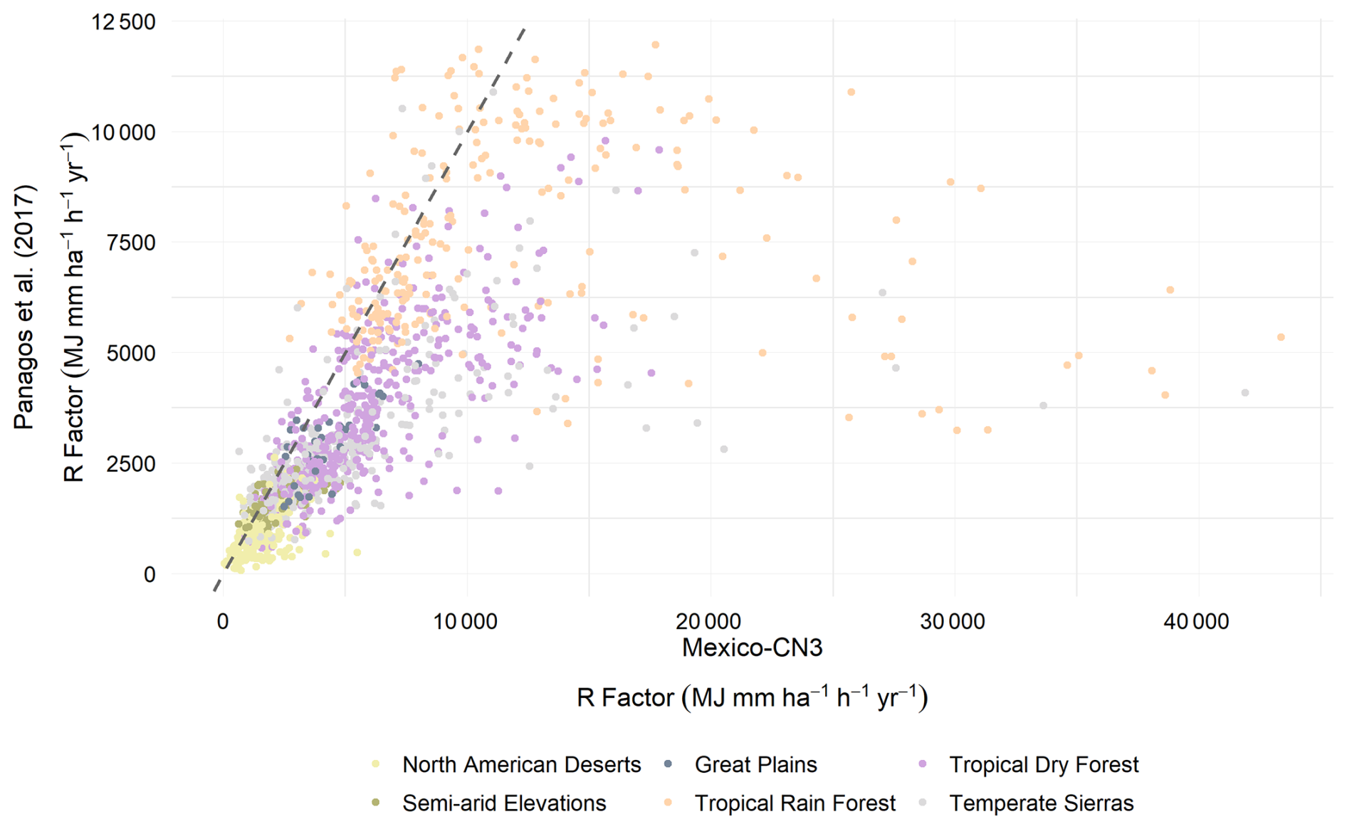
Figure 9Scatter plot of R factor values from the global rainfall erosivity surface from Panagos et al. (2017) and the R factor estimated with the Richardson et al. (1983) power law equation with the rainfall time series of the Mexico-CN3 (1988–2017) database.
4.4 Future research directions
Now, we present our perspective on future directions for cost effective modeling and mapping rainfall erosivity patterns and trends across Mexico along with four main interoperability barriers: (a) transitioning into high temporal resolution and to sub hourly dynamics, (b) climate change projections and non stationarity, (c) integration with digital soil mapping and soil organic carbon sequestration models and (d) uncertainty quantification and the role of citizen science.
First, while the current database provides a robust baseline for the R factor in Mexico, future research could prioritise the integration of sub-hourly rainfall intensity data. The increasing availability of automated weather station networks and high-resolution satellite products (such as GPM-IMERG) offers a pathway to characterise soil erosivity with increased accuracy (Yin et al., 2017; Yan et al., 2025; Lobo and Bonilla, 2015). Transitioning from daily aggregates to event-based modeling will allow for a deeper understanding of how extreme, short-duration convective storms, which are common in Mexico's complex topography, contribute disproportionately to annual soil loss.
Second, rainfall erosivity projections are commonly based on stationarity assumptions (Vantas et al., 2020); a critical frontier involves the incorporation of non-stationarity into erosivity mapping. As climate change alters the frequency and intensity of tropical cyclones and North American Monsoon patterns, static historical averages may become less predictive (Almagro et al., 2017; Wang et al., 2023a; Zhang et al., 2010). Future modeling efforts could couple the current R factor baseline with CMIP6 climate projections to develop digital scenarios of future erosivity patterns and trends. This will be essential for designing long-term sustainable land management strategies and adapting hydraulic infrastructure to a more aggressive erosive environment.
Third, there is a significant opportunity to integrate rainfall erosivity databases with digital soil mapping frameworks to evaluate the positive and negative feedbacks between erosion and soil organic carbon dynamics (Song et al., 2026; Min et al., 2026; Qiao et al., 2025). Future studies could focus on the soil carbon losses in response to soil erosion and sediment transport across different geomorphic positions (Sun et al., 2024; Silva et al., 2016). By coupling high-resolution erosivity maps with national soil property grids, researchers can better quantify the role of water erosion in carbon redistribution, moving Mexico toward a more comprehensive National Soil Monitoring System (Abbruzzini et al., 2026; Guerrero et al., 2014; Varón-Ramírez and Guevara, 2024).
Fourth, future iterations of the Mexican rainfall erosivity database should focus on rigorous uncertainty quantification e.g., using Bayesian frameworks or ensemble modeling. Given the uneven distribution of primary weather stations across Mexico's complex and diverse terrain, identifying regions with high predictive uncertainty is paramount. Furthermore, the integration of “Citizen Science” and low-cost IoT (Internet of Things) recording rain gauge could serve as a useful validation tool. Engaging local communities in data collection would not only fill geographic gaps but also bridge the divide between high-level modeling and on-the-ground soil conservation practices (Duwal et al., 2025; Dawoud et al., 2023; Tedla et al., 2022).
Following the FAIR principles for scientific data, we published the resulting rainfall erosivity databases (Mexico-CN1 1968–1997, Mexico-CN2 1978–2007, and Mexico-CN3 1988–2017) together with the completed daily rainfall time series for the three climate normals in the Environmental Data Initiative (EDI) repository at https://doi.org/10.6073/pasta/dd2b30e28ee25ff2d60d8a9f43 6951d2 (Varón-Ramírez et al., 2026).
The rainfall erosivity databases contain station metadata, including weather station code, name, geographic coordinates, altitude, and ecoregion, as well as indicators associated with the homogenization and gap-filling procedures, such as the Root Mean Square Error (RMSE) and the percentage change in the rainfall time series. Additionally, the databases include mean annual rainfall, the accumulated number of erosive rainfall days, and rainfall erosivity estimates derived from the empirical models proposed by Richardson et al. (1983), Liu et al. (2020) and Xie et al. (2016).
The daily rainfall databases contain quality-controlled, homogenized, and gap-filled daily rainfall time series for 1369; 1678; and 1676 weather stations corresponding to the 1968–1997, 1978–2007, and 1988–2017 climate normals, respectively. Each rainfall time series is identified by a unique weather station code and includes flags associated with the quality-control and homogenization procedures.
Rproject scripts to reproduce the workflow described in this research is available at https://doi.org/10.5281/zenodo.15468097 (Varón-Ramírez, 2025).
We present the first harmonized rainfall and rainfall erosivity database for Mexico, developed from legacy climate data and covering the period from 1968 to 2017. Our workflow included complete quality control and homogenization processes to ensure data quality for 1369; 1678: and 1676 rainfall time series data and rainfall erosivity for three climate normals (1968–1997, 1978–2007, and 1988–2017), respectively. This is a climatological database that substantially improves the spatial representation and documentation of erosivity patterns compared to global and local products.
Results revealed a strong climatic and geographical control on erosivity patterns. Tropical humid regions, particularly the Isthmus of Tehuantepec, southern Mexico, and portions of the Pacific coastal zone, exhibited the highest erosivity values, whereas the arid and semi-arid regions of northern Mexico showed the lowest erosive potential. These patterns are consistent with the broader global tendency for extreme erosivity to occur in humid tropical environments.
The sensitivity analysis indicates that the homogenization and gap-filling procedures may locally modify rainfall erosivity estimates, particularly in stations with low-quality or highly inhomogeneous rainfall records. However, despite these local variations, the general spatial patterns and ecoregional contrasts of rainfall erosivity remained stable across the three climate normals. These results suggest that the homogenization process effectively corrected station-specific inconsistencies while preserving the broader climatic structure of rainfall erosivity across Mexico.
The new database provides an important foundation for national-scale soil erosion assessments and improves the representation of rainfall forcing for RUSLE-based applications, land degradation studies, hydrological analyses, and climate-related environmental research. In addition, the open availability of the database under FAIR principles facilitates its use by researchers, technical agencies, students, and decision-makers interested in rainfall dynamics and soil erosion processes in Mexico.
Future efforts should focus on incorporating high-temporal-resolution rainfall observations from automatic weather stations, strengthening institutional data-sharing initiatives, and developing spatially explicit erosivity prediction models using geostatistical and machine learning approaches. These advances would further improve the accuracy of rainfall erosivity estimation and contribute to more robust soil erosion assessments under changing climatic conditions.
Table A1Identification of the number of rainfall time series with consecutive zero and NA values.
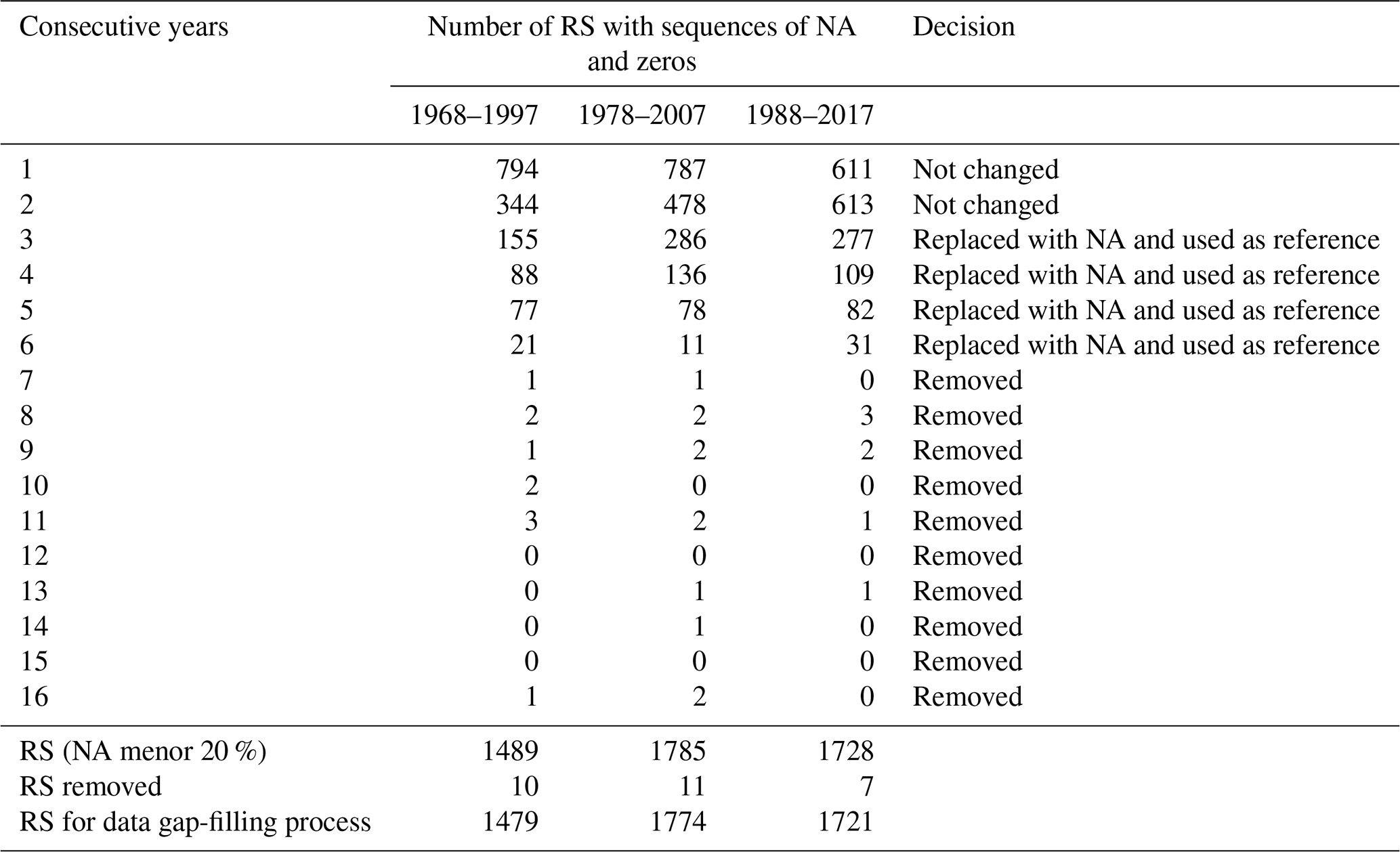
Table A2Homogenization parameters for monthly series. Eco: Ecoregion (1: Mediterranean California, 2: North American Deserts, 3: Semi-arid Elevations, 4: Great Plains, 5: Tropical Rain Forest, 6: Tropical Dry Forest, 7: Temperate Sierras); inht: threshold values used to identify break points in the Standard Normal Homogeneity Test (SNHT); dz.max and dz.min (upper and lower): standard deviations to consider suspicious and anomalous data.
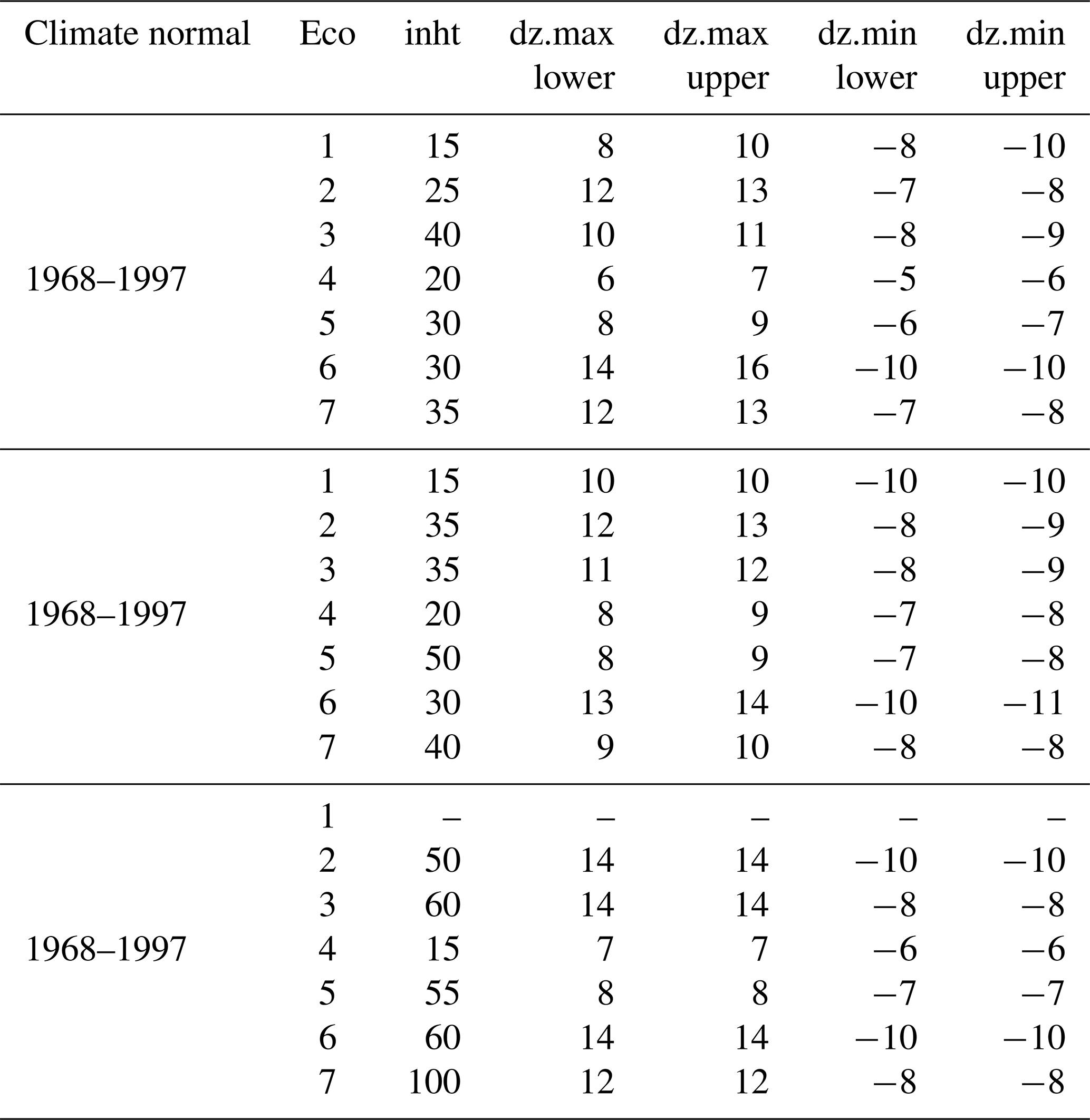
Table A3Homogenization parameters for daily rainfall time series by ecoregion and group. Eco: Ecoregion (2: North American Deserts, 3: Semi-arid Elevations, 5: Tropical Rain Forest, 6: Tropical Dry Forest, 7: Temperate Sierras); RS: Number of rainfall time series; inht: threshold values used to identify break points in the Standard Normal Homogeneity Test (SNHT); dz.max and dz.min (upper and lower): standard deviations to consider suspicious and anomalous data.
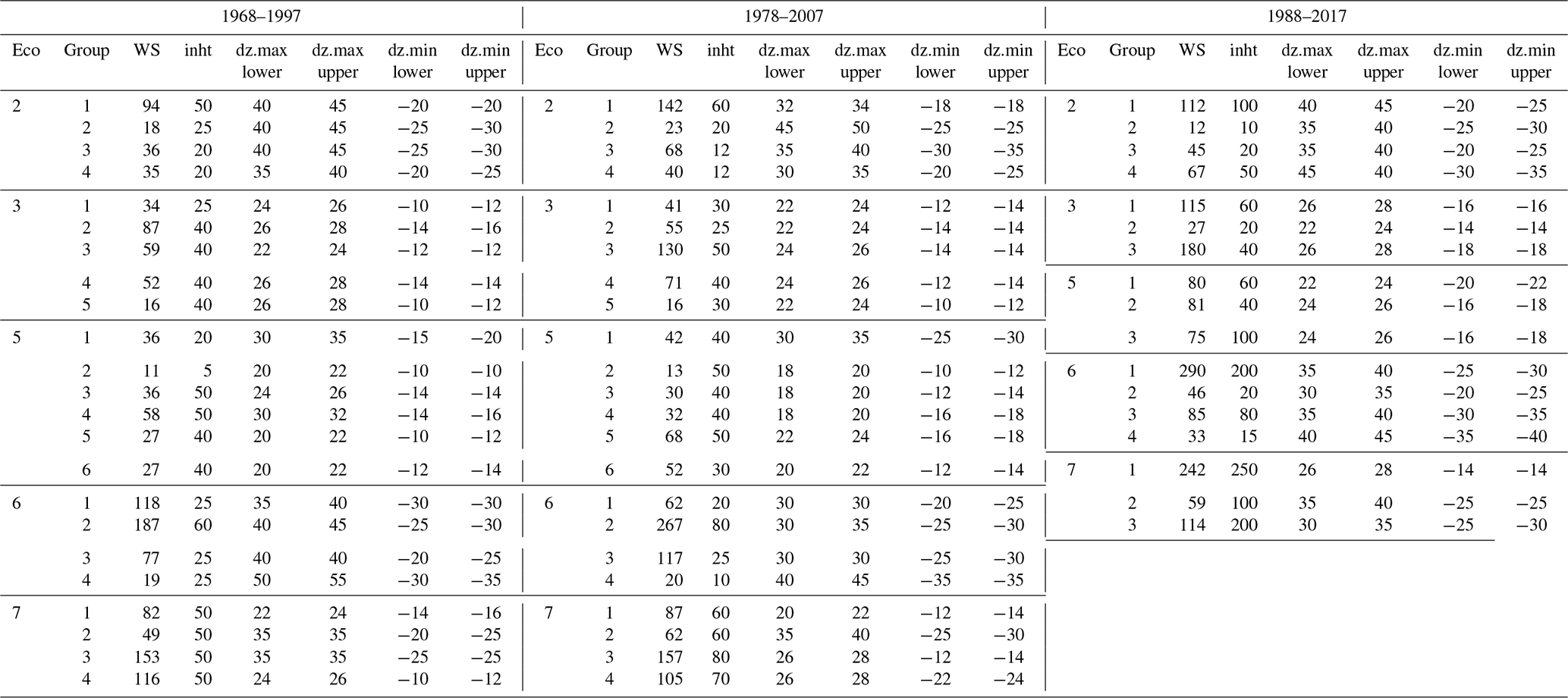
Table A4Monthly climatological deviation introduced by the gap-filling process by month and ecoregion (metric RMSE in mm). Eco: Ecoregion (1: Mediterranean California, 2: North American Deserts, 3: Semi-arid Elevations, 4: Great Plains, 5: Tropical Rain Forest, 6: Tropical Dry Forest, 7: Temperate Sierras). Bold values correspond to the highest totals by month and ecoregions.
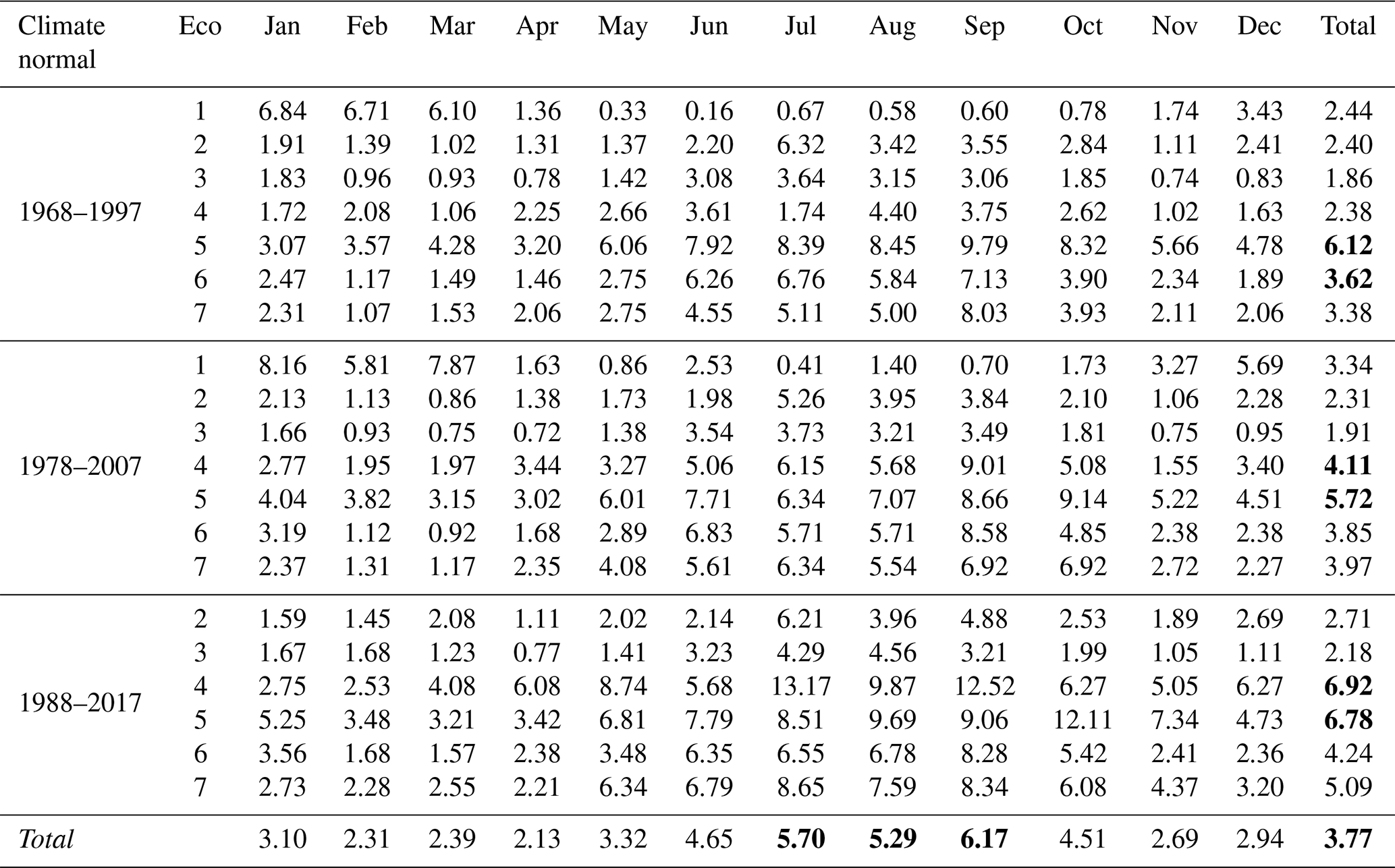
Table A5Mean rainfall erosivity and mean percentage change in erosivity by ecoregion for the three climate normals. Percentage changes were estimated from modifications to the rainfall time series resulting from the gap-filling and homogenization processes. Eco: Ecoregion (1: Mediterranean California, 2: North American Deserts, 3: Semi-arid Elevations, 4: Great Plains, 5: Tropical Rain Forest, 6: Tropical Dry Forest, 7: Temperate Sierras).
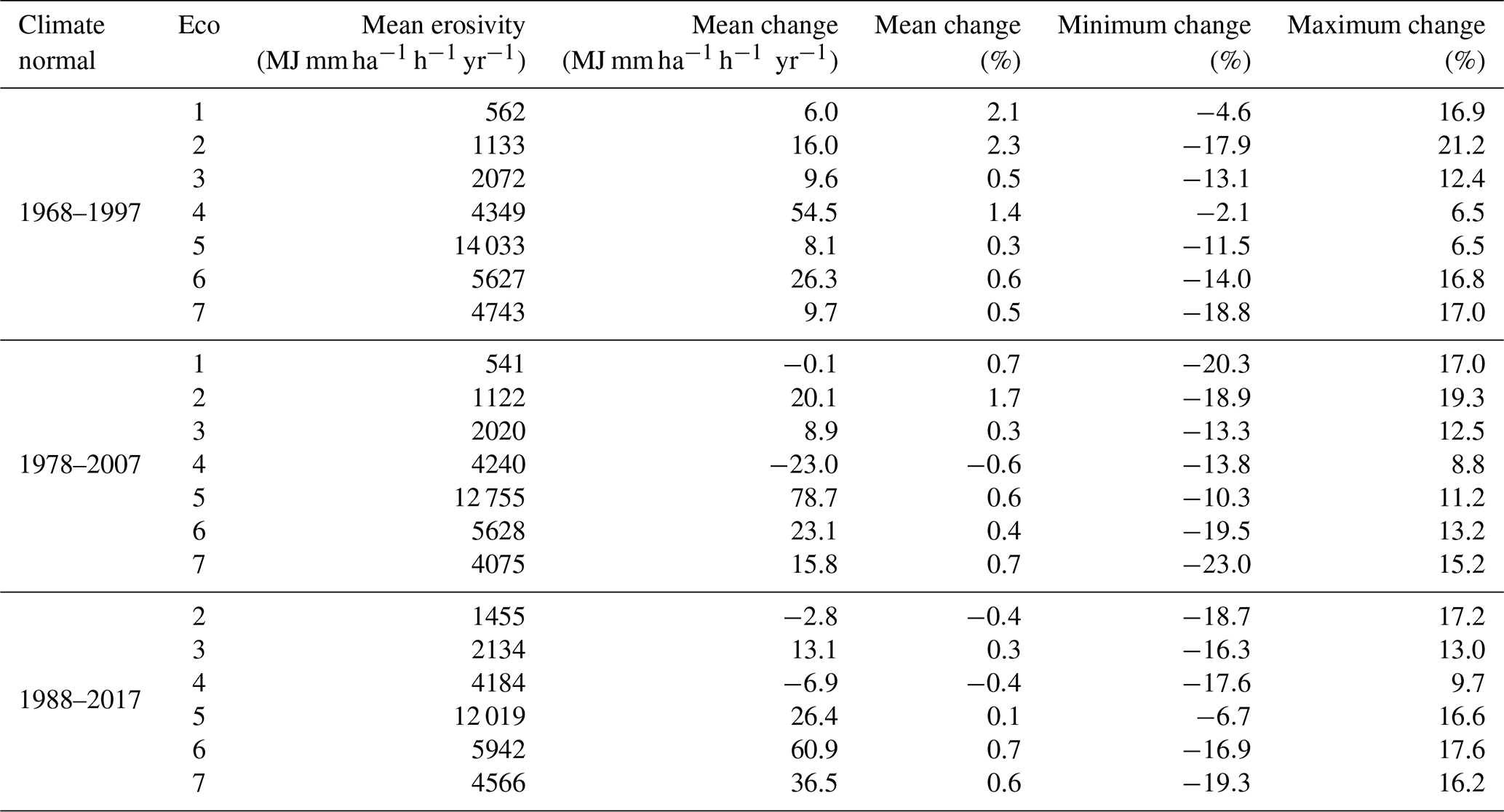
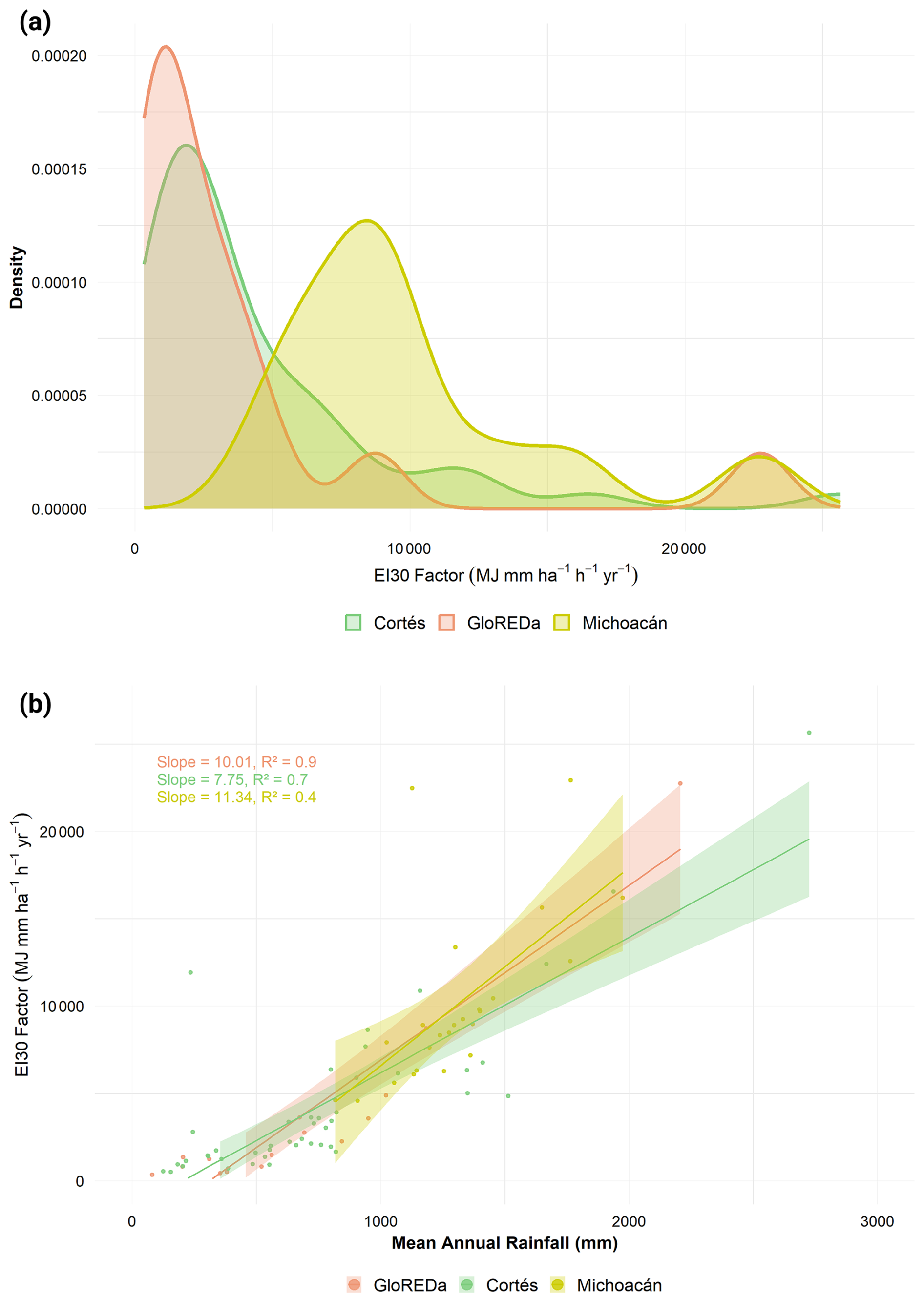
Figure A1Characteristics of the three validations databases: GloREDa, Cortés, and Michoacán. (a) Density plot of EI30 values; (b) linear relationship between EI30 and the mean annual rainfall.
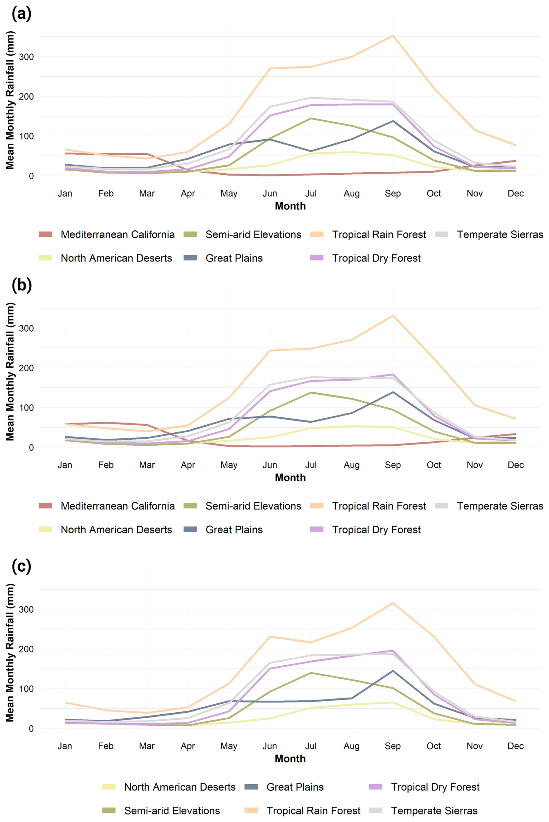
Figure A2Mean monthly rainfall for all seven ecoregions. (a) Climate normal (CN1) 1968–1997; (b) climate normal (CN2) 1978–2007; and (c) climate normal (CN3) 1988–2017.
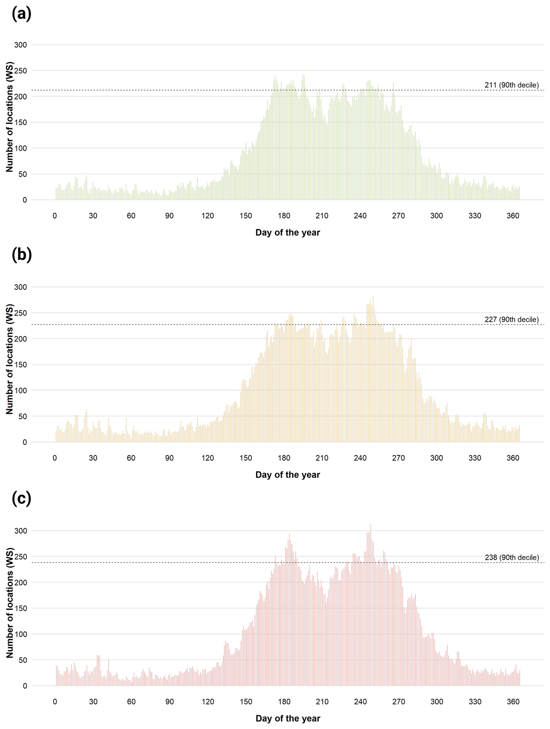
Figure A3Number of locations with erosive rainfall of each day of the year for the three climate normal, (a) 1968–1997, (b) 1978–2007, and (c) 1988–2017.
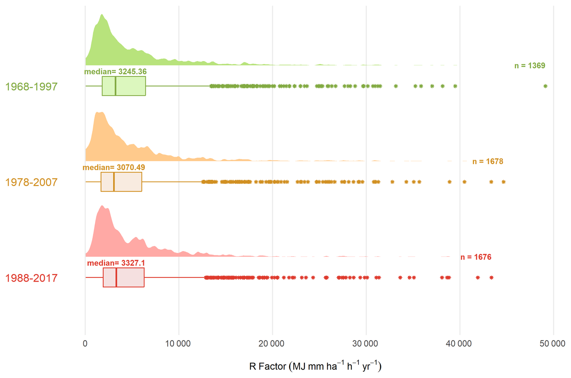
Figure A4Density plot and Box-Plot of erosivity factor (R) calculated from daily rainfall time series for the three climate normals.
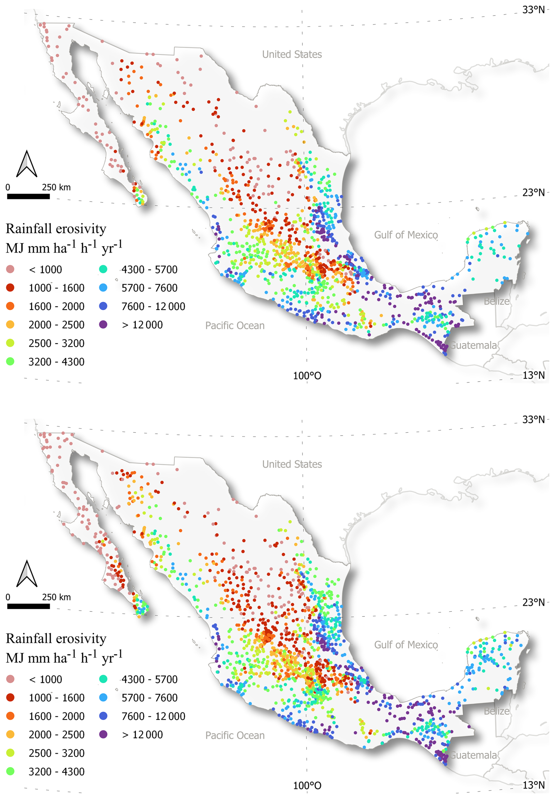
Figure A5R factor values calculated with the power law equation proposed by (Richardson et al., 1983) at daily resolution. Upper panel: climate normal 1968–1997. Bottom panel: climate normal 1978–2007. The legend classes approximately represent deciles of the statistical distribution, although not exactly.
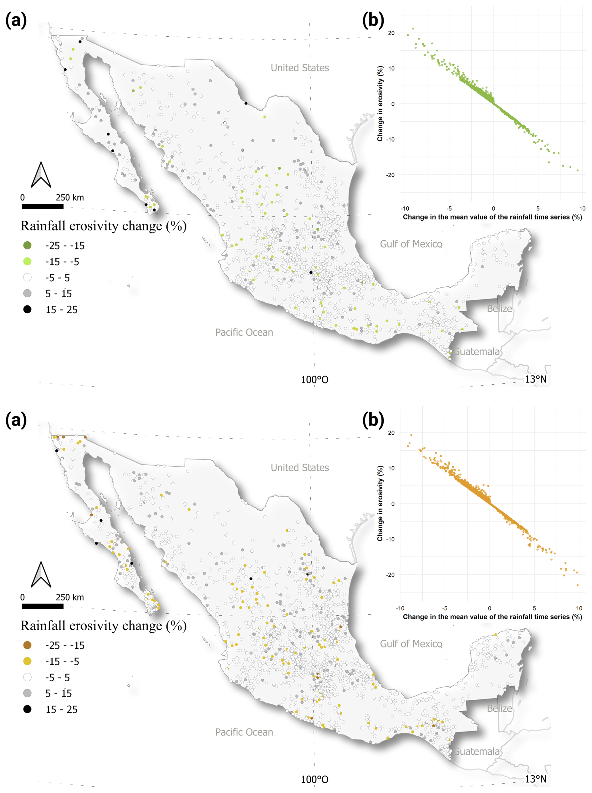
Figure A6Percentage changes in rainfall erosivity after modifying precipitation time series according to the percentage change in the mean value of the rainfall time series before and after the gap-filling and homogenization processes. Upper panel: climate normal 1968–1997. Bottom panel: climate normal 1978–2007. (a) Spatial distribution of percentage changes in rainfall erosivity. (b) Relationship between percentage changes in the mean value of the rainfall time series and percentage changes in rainfall erosivity.
This supplementary material presents translated excerpts from the Materials and Methods section of the master's thesis by Cortés (1991), Caracterización de la erosividad de la lluvia en México utilizando métodos multivariados, developed at the Colegio de Posgraduados (Montecillo, Mexico) in 1991. These excerpts describe the procedures used to construct the rainfall erosivity dataset employed in this study as a validation dataset. Because the original thesis is only available in physical format and written in Spanish, the most relevant sections were translated into English to facilitate understanding and reproducibility for non-Spanish-speaking readers. The translated material includes the procedures for pluviogram reading, rainfall event definition, and calculation of rainfall intensities and the EI30 index. A physical copy of the thesis is available at the Colegio de Posgraduados library, and the catalog information can be accessed at (http://catalogo.colpos.mx/cgi-bin/koha/opac-detail.pl?biblionumber=17230, last access: 7 May 2026). A complete scanned PDF version of the original thesis is available from the authors upon request.
-
Pages 11–13
III. LITERATURE REVIEW
3.3.2.1. Wischmeier Index (EI30)
The EI30 index was proposed by Wischmeier (1959) and is defined as the product of the total kinetic energy of rainfall (E) and the maximum 30 min intensity (I30). It measures the effect in which erosion caused by splash detachment and flow turbulence combine with runoff to remove detached soil particles from the land surface. This process is known as sheet erosion. Its calculation is performed using the following equation:
where EI30 is the erosivity index for a rainfall event (MJ mm ha−1 h−1). E is the total kinetic energy of rainfall (MJ ha−1). I30 is the maximum rainfall intensity in 30 minutes (mm h−1).
The kinetic energy of rainfall is obtained using the equation:
where ej is the kinetic energy for the time interval j (MJ ha−1 mm−1). Pj is the amount of rainfall during the time interval j (mm). n is the number of intervals with different intensity during the same event.
The calculation of ej in units of the International System is carried out using the equation Wischmeier and Smith, 1978; Foster et al., 1981:
where Ij is the rainfall intensity during interval j (mm h−1); , tj is the duration of interval j (minutes) and ej and Pj were already defined.
The multiplication by (60) converts the data into hourly units. The value of ej becomes constant for I>76 mm h−1 because it is considered that, at higher intensities, the size of raindrops no longer increases (Wischmeier and Smith, 1978).
The sum of the EI30 values during 1 year forms the annual rainfall erosivity factor (R) of the Universal Soil Loss Equation (USLE), proposed by Wischmeier and Smith (1978) and expressed as:
where A is the average annual soil loss (t ha−1), R is the rainfall erosivity factor (MJ ha−1 h−1), K is the soil erodibility factor (t ha h MJ−1 mm−1 ha−1), L is the slope length factor (dimensionless), S is the slope steepness factor (dimensionless), C is the crop management factor (dimensionless), and P is the support practice factor for erosion control (dimensionless)
The algebraic expression of R is therefore:
where R is the rainfall erosivity factor or annual erosivity index (MJ mm ha−1 h−1 yr−1) and m is the number of rainfall events during the year.
The EI30 has proven to be an efficient rainfall erosivity index for estimating soil loss in different parts of the world, although originally developed for the region east of the Rocky Mountains in the United States. In other cases, however, Lal (1979), Roose (1979), Hudson (1981), the correlations between EI30 and soil loss have been low, and better results have been found when considering other approaches, thus obtaining other erosivity indices.
-
Pages 40 and 43–45
IV. MATERIALS AND METHODS
4.1 Materials
The materials used were: daily-recording pluviograms, digitizing tablets, microcomputers, and floppy disks for microcomputers. The statistical analysis of the information was carried out using the SAS, STATGRAPHICS, and GEOEAS statistical packages. The latter, perhaps less widely known than the previous two, is a geostatistical package (Geostatistical Environmental Assessment Software: GEOEAS) developed by the US EPA Environmental Monitoring Systems Laboratory in Las Vegas, Nevada, in cooperation with the Department of Applied Earth Sciences at Stanford University. It is useful for interpolation studies because, in addition to allowing the calculation of basic statistics and scatterplots of variables, it generates variograms for one or more variables in bidimensional space, enables validation of such variograms, and based on them, kriging can be performed (estimating values for a grid of points). It also has the capability to generate contour maps of isovalues for the variable of interest. Harvard Graphics was also used in the preparation of some figures and graphs. The programs used for data acquisition and information processing were written in BASIC and PASCAL programming languages.
4.2 Methodology
4.2.1 Data acquisition, organization, and classification
The development of the present work was based on the analysis of pluviograms provided by the National Meteorological Service (SMN). The number and names of the stations are presented in Table 4.2.1, and their location can be seen in Fig. 4.2.1.
The selection of stations was based on the assumption that a greater number of years analyzed would produce more reliable results, as shown by the experience of studies conducted in different parts of the world related to rainfall erosivity. Thus, it was found that although there is no number of years defined as a minimum, there is consensus (Stocking and Elwell, 1976; Moldenhauer, 1980) that a period equal to or greater than 20 years would be desirable.
Finally, the determining factor appears to be data availability, and as expected, developing countries generally do not have the same number and equipment of meteorological stations available in more developed countries. While Koolhaas (1979) presents an isoerodent map (lines connecting points with equal mean annual rainfall erosivity) for Uruguay based on the analysis of pluviograms from a single meteorological station (and estimated values for another 100 stations using a regression equation), the isoerodent map for the United States (Koolhaas, 1979) was obtained from the analysis of 181 pluviographs (estimating values for another 1700 locations using a regression equation).
Based on the above, and also considering that the work to be carried out is laborious, it was decided to analyze an uninterrupted 11-year period of rainfall data from 1977 to 1987, inclusive. However, the number of stations in Mexico meeting this requirement is quite limited (approximately 20 were found within the SMN), and their spatial distribution across the national territory is deficient. Consequently, it was necessary to make considerations regarding the minimum number of years of available information (pluviograms) that each station should fulfill. Therefore, it was decided to accept 51 stations that had a minimum of four consecutive years of data records. Finally, the Ceicades-CP station (53) in Cárdenas, Tabasco, with only one year of information, and Ocozocuatla, Chiapas (52), with six non-consecutive years of information, were included because the sample coverage in that area was very poor and it was desirable to have some reference data for the region. It was also found that the stations of Santa Rosalía, Baja California Sur; Cuernavaca, Morelos; Puerto Ángel, Oaxaca; and Tapachula, Chiapas, did not strictly meet the aforementioned restrictions, since they lacked one month of data (Cuernavaca lacked two months) within the four-year historical period. Nevertheless, despite the above, these stations were also included in the analysis.
In total, information from 53 meteorological stations was used. Table A1 in the Appendix presents the years analyzed for each station.
4.2.2. Reading of pluviograms
For the reading of pluviograms, all rainfall events were considered, regardless of how small the precipitation depth was; therefore, every event recorded by the pluviograph was taken into account in the study.
To perform the reading process, the PLUVIOGRAMAS program in Applesoft BASIC for the Apple II microcomputer was used. In combination with a digitizing tablet, the program allowed the coordinates of the pluviograph chart to be read and subsequently performed the required calculations (the program can be consulted in the work of Cortés, 1987).
To define an individual rainfall event or storm, the criterion proposed by Wischmeier (1959) was followed. In developing the EI30 erosivity index, he found better results when a rainfall event was considered independent from another only if there was a rainless interval of 6 or more hours between them.
4.2.3. Procedure for calculating maximum rainfall intensities and erosivity indices
The calculation of maximum rainfall intensities for different duration periods (5, 10, 15, 30, 45, 60, 90, and 120 min) and erosivity indices was performed using the previously mentioned PLUVIOGRAMAS program. The procedure used to determine maximum rainfall intensities is presented below.
The different intensities within a particular rainfall event were determined using the time (t) and rainfall depth (h) coordinates at the points where the slope of the curve traced by the pluviograph changed. Using these intensities (I), an array was generated to obtain the maximum intensities for durations of 5, 10, 15, 30, 45, 60, 90, and 120 min. The calculation is described by the following algorithm.
The maximum intensity (Imax) for a duration of Ti minutes is:
where i is the position of the intensities (I) selected together with their respective duration (d). Example: i=1 is assigned to the highest intensity, i=2 to the second highest intensity, and so on in descending order of magnitude, searching above and below the highest intensity. n is the position of the last intensity that must be selected because its respective duration added to the previous one exceeds Ti (or is equal to Ti). Thus, the duration taken from this last intensity is the number of minutes necessary to complete Ti.
For the calculation of erosivity indices, the corresponding equations are incorporated into the program, as described in Sect. 3.3.2 of the Literature Review. The indices are calculated for each storm event; therefore, by summing the values occurring within a month, the monthly value is obtained; if all the values for a year are summed, the annual value is obtained.
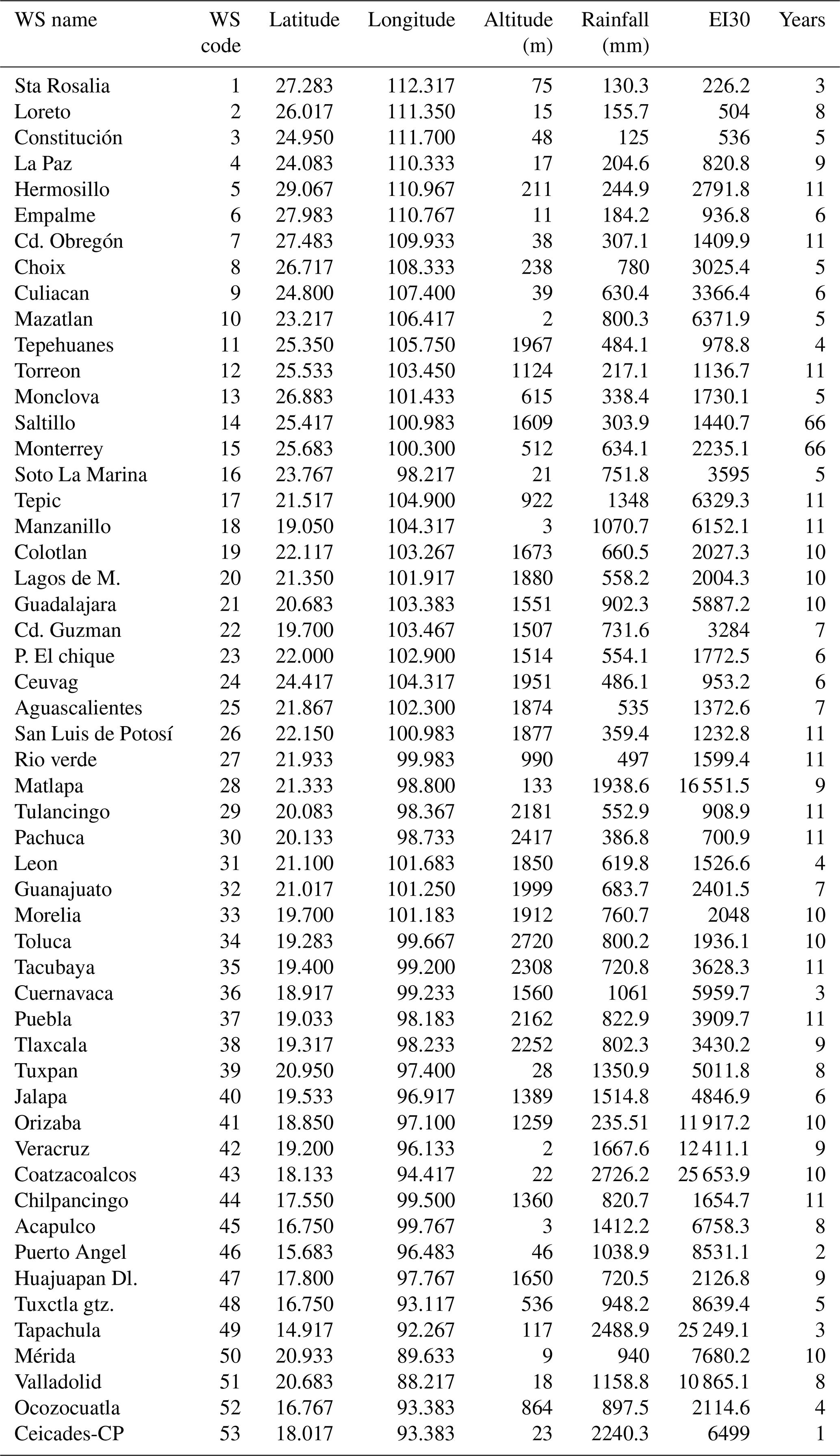
VMVR, DAGL, and MG contributed with conceptualization, formal analysis, Methodology, and visualization. VMVR, DAGL, and CEAC contributed to the data curation and writing – original draft preparation. CEAC, AGT, BLPP, DLL, RRGLL, and MG contributed to Project administration, writing, review, and editing. VMVR, BLPP, and MG contributed to funding acquisition.
The contact author has declared that none of the authors has any competing interests.
Publisher's note: Copernicus Publications remains neutral with regard to jurisdictional claims made in the text, published maps, institutional affiliations, or any other geographical representation in this paper. The authors bear the ultimate responsibility for providing appropriate place names. Views expressed in the text are those of the authors and do not necessarily reflect the views of the publisher.
This research has been supported by Conahcyt (now SECIHTI) CF-2023I-1846, UNESCO-IGCP#765, UNAM-PAPIIT #IG101325, and UNAM-PAPIME #PE109326.
This paper was edited by Di Tian and reviewed by Paulina I. Ponce-Philimon and one anonymous referee.
Viviana Marcela Varón-Ramírez and Carlos Eduardo Arroyo-Cruz acknowledged support from SECIHTI scholarship (PhD level, CVU: 1240028, 1268803, respectively). Viviana Marcela Varón-Ramírez acknowledges the Corporacióó Colombiana de Investigación Agropecuaria (AGROSAVIA) for granting a study leave. The authors want to thank the National Meteorological Service (SMN by its initials in Spanish) and the National Water Commission (CONAGUA by its initials in Spanish) for making the national climate data publicly available.
Abbruzzini, T. F., Figueroa, D., Cruz, C. E. A., Varón-Ramírez, V. M., Santamaria, M. A. G., and Prado, B.: Assessing soil nutrient spatial variability in Mexico through digital soil mapping: Implications for sustainable agriculture, Geoderma Reg., 45, e01081, https://doi.org/10.1016/j.geodrs.2026.e01081, 2026. a
Adeyeri, O., Lamptey, B., Lawin, A., and Sanda, I.: Spatio-Temporal Precipitation Trend and Homogeneity Analysis in Komadugu-Yobe Basin, Lake Chad Region, J. Climatol. Weather Forecast., 5, https://doi.org/10.4172/2332-2594.1000214, 2017. a
Adeyeri, O., Laux, P., Ishola, K., Zhou, W., Balogun, I., Adeyewa, Z., and Kunstmann, H.: Homogenising meteorological variables: Impact on trends and associated climate indices, J. Hydrol., 607, 127585, https://doi.org/10.1016/j.jhydrol.2022.127585, 2022. a, b
Agustín Breña-Naranjo, J., Pedrozo-Acuña, A., Pozos-Estrada, O., Jiménez-López, S. A., and López-López, M. R.: The contribution of tropical cyclones to rainfall in Mexico, Phys. Chem. Earth Pt. A/B/C, 83–84, 111–122, https://doi.org/10.1016/j.pce.2015.05.011, 2015. a
Alexandersson, H.: A homogeneity test applied to precipitation data, J. Climatol., 6, 661–675, https://doi.org/10.1002/joc.3370060607, 1986. a
Almagro, A., Oliveira, P. T. S., Nearing, M. A., and Hagemann, S.: Projected climate change impacts in rainfall erosivity over Brazil, Sci. Rep., 7, 8130, https://doi.org/10.1038/s41598-017-08298-y, 2017. a
Beck, H. E., Zimmermann, N. E., McVicar, T. R., Vergopolan, N., Berg, A., and Wood, E. F.: Present and future Köppen–Geiger climate classification maps at 1-km resolution, Sci. Data, 5, 180214, https://doi.org/10.1038/sdata.2018.214, 2018. a
Benites, E. T., Becerra, J. C., Gil, J. U., Cedillo, L. T., and Torres, P. S. R.: Predicción de la erosión hídrica en la cuenca del Cañón del Sumidero, Chiapas, Revista Mexicana de Ciencias Agrícolas, 11, 1903–1915, https://doi.org/10.29312/remexca.v11i8.2747, 2020. a
Bezak, N., Borrelli, P., and Panagos, P.: Exploring the possible role of satellite-based rainfall data in estimating inter- and intra-annual global rainfall erosivity, Hydrol. Earth Syst. Sci., 26, 1907–1924, https://doi.org/10.5194/hess-26-1907-2022, 2022. a
Bolaños González, M. A., Paz Pellat, F., Cruz Gaistardo, C. O., Argumedo Espinoza, J. A., Romero Benítez, V. M., and de la Cruz Cabrera, J. C.: Mapa de erosión de los suelos de México y posibles implicaciones en el almacenamiento de carbono orgánico del suelo, Terra Latinoamericana, 34, 271–288, 2016. a
Boos, W. R. and Pascale, S.: Mechanical forcing of the North American monsoon by orography, Nature, 599, 611–615, https://doi.org/10.1038/s41586-021-03978-2,2021. a
Borrelli, P., Robinson, D., Fleischer, L. R., Lugato, E., Ballabio, C., Alewell, C., Meusburger, M., Modugno, P., Schütt, M., Tenuta, K. E., and Panagos, P.: Land use and climate change impacts on global soil erosion by water (2015–2070), P. Natl. Acad. Sci. USA, 117, 21994–22001, https://doi.org/10.1073/pnas.2001403117, 2020. a
Borrelli, P., Ballabio, C., Yang, J. E., Robinson, D. A., and Panagos, P.: GloSEM: High-resolution global estimates of present and future soil displacement in croplands by water erosion, Sci. Data, 9, 406, https://doi.org/10.1038/s41597-022-01489-x, 2022. a
Cardoso, D. P., Silva, E. M., Avanzi, J. C., Muniz, J. A., Ferreira, D. F., Silva, M. L. N., Acuña-Guzman, S. F., and Curi, N.: RainfallErosivityFactor: An R package for rainfall erosivity (R-factor) determination, Catena, 189, 104509, https://doi.org/10.1016/j.catena.2020.104509, 2020. a
Carrera, J. J., Levresse, G. P., and Hernández-Espriú, J. A.: Geostatistical Analysis of Yearly Precipitation at the National Level: Stratification and Anisotropy Considerations in Mexico, SSRN [preprint], https://doi.org/10.2139/ssrn.4820011, 2024. a
Carrera-Hernández, J. J.: Mexico's High Resolution Climate Database (MexHiResClimDB): a new daily high-resolution gridded climate dataset for Mexico covering 1951–2020, Earth Syst. Sci. Data, 17, 6911–6941, https://doi.org/10.5194/essd-17-6911-2025, 2025. a, b, c, d, e
Chen, Y., Xu, M., Wang, Z., Chen, W., and Lai, C.: Reexamination of the Xie model and spatiotemporal variability in rainfall erosivity in mainland China from 1960 to 2018, Catena, 195, 104837, https://doi.org/10.1016/j.catena.2020.104837, 2020. a
Commission for Environmental Cooperation: Ecological Regions of North America – Toward a Common Perspective, Commission for Environmental Cooperation, Montreal, Canada, ISBN 2-922305-20-1, 1997. a, b, c
Cortés T., H. G.: Análisis de la distribución estadística de las intensidades de área estudio del CREZAS-CP, Tesis profesional, Depto. de Irrigación, UACH, Chapingo, Mex., p. 128, 1987. a
Cortés, H. G.: Caracterización de la erosividad de la lluvia en México utilizando métodos multivariados, MS thesis, Colegio de Posgraduados, Montecillo, Mexico, centro de Edafología, MS thesis, http://www.biblio.colpos.mx/portal/ (last access: 25 June 2026), 1991. a, b, c, d, e, f, g, h, i
Cuervo-Robayo, A. P., Téllez-Valdás, O., Gómez-Albores, M. A., Venegas-Barrera, C. S., Manjarrez, J., and Martínez-Meyer, E.: An update of high-resolution monthly climate surfaces for Mexico, Int. J. Climatol., 34, 2427–2437, https://doi.org/10.1002/joc.3848, cited by: 153, 2014. a, b, c
Cuervo-Robayo, A. P., Ureta, C., Gómez-Albores, M. A., Meneses-Mosquera, A. K., Téllez-Valdés, O., and Martínez-Meyer, E.: One hundred years of climate change in Mexico, PLOS ONE, 15, 1–19, https://doi.org/10.1371/journal.pone.0209808, 2020. a
Das, S., Jain, M. K., Gupta, V., McGehee, R. P., Yin, S., de Mello, C. R., Azari, M., Borrelli, P., and Panagos, P.: GloRESatE: A dataset for global rainfall erosivity derived from multi-source data, Sci. Data, 11, 926, https://doi.org/10.1038/s41597-024-03756-5, 2024. a, b, c, d
Dawoud, O., Eljamassi, A., and Abunada, Z.: Mapping and Quantification of Soil Erosion and Sediment Delivery in Poorly Developed Urban Areas: A Case Study, Sustainability, 15, https://doi.org/10.3390/su151813683, 2023. a
de Anda Sánchez, J.: Precipitation in Mexico, Springer International Publishing, Cham, ISBN 978-3-030-40686-8, 1–14, https://doi.org/10.1007/978-3-030-40686-8_1, 2020. a, b
Deitch, M. J., Sapundjieff, M. J., and Feirer, S. T.: Characterizing Precipitation Variability and Trends in the World's Mediterranean-Climate Areas, Water, 9, https://doi.org/10.3390/w9040259, 2017. a
Dunkerley, D. L.: Rainfall intensity bursts and the erosion of soils: an analysis highlighting the need for high temporal resolution rainfall data for research under current and future climates, Earth Surf. Dynam., 7, 345–360, https://doi.org/10.5194/esurf-7-345-2019, 2019. a
Duwal, S., Prajapati, R., Upadhyay, S., Neupane, S., Lakhe, H., Thapa, B. R., Davids, J. C., and Talchabhadel, R.: Leveraging a Citizen Science Approach for Rainfall Monitoring: Evaluating Performance and Reliability To Complement Standard Datasets, Earth Syst. Environ., https://doi.org/10.1007/s41748-025-00920-8, in press, 2025. a
Efthimiou, N.: Evaluating the performance of different empirical rainfall erosivity (R) factor formulas using sediment yield measurements, Catena, 169, 195–208, https://doi.org/10.1016/j.catena.2018.05.037, 2018. a
Feng, Z., Zhang, Z., Zuo, Y., Wan, X., Wang, L., Chen, H., Xiong, G., Liu, Y., Tang, Q., and Liang, T.: Analysis of long term water quality variations driven by multiple factors in a typical basin of Beijing-Tianjin-Hebei region combined with neural networks, J. Clean. Product., 382, 135367, https://doi.org/10.1016/j.jclepro.2022.135367, 2023. a
Fenta, A. A., Tsunekawa, A., Haregeweyn, N., Yasuda, H., Tsubo, M., Borrelli, P., Kawai, T., Sewale Belay, A., Ebabu, K., Liyew Berihun, M., Sultan, D., Asamin Setargie, T., Elnashar, A., and Panagos, P.: Improving satellite-based global rainfall erosivity estimates through merging with gauge data, J. Hydrol., 620, https://doi.org/10.1016/j.jhydrol.2023.129555, 2023. a
Foster, G. R., McCool, D. K., Renard, K. G., and Moldenhauer, W. C.: Conversion of the universal soil loss equation to SI metric units, J. Soil Water Conserv., 36, 355–359, 1981. a
Fransiska, H., Agustina, D., Setyorini, D., Sumartajaya, I. M., and Kurnia, A.: Time Series Clustering Analysis Using Dynamic Time Warping Technique of DailyRainfall in Bengkulu Province, IOP Conf. Ser.: Earth and Environ. Sci., 1359, 012026, https://doi.org/10.1088/1755-1315/1359/1/012026, 2024. a
García, E.: Climas (clasificación de Köppen, modificado por García), Map, scale , México, http://www.conabio.gob.mx/informacion/gis/ (last access: 10 April 2026), 1998. a, b
Gochis, D. J., Brito-Castillo, L., and Shuttleworth, W. J.: Hydroclimatology of the North American Monsoon region in northwest Mexico, J. Hydrol., 316, 53–70, https://doi.org/10.1016/j.jhydrol.2005.04.021, 2006. a, b
Gómez-Latorre, D. A., Araujo-Carrillo, G. A., and Leguizamón, Y. R.: Regionalización de patrones de lluvias para períodos multianuales secos y húmedos en el Altiplano Cundiboyacense de Colombia, Revista de Climatología, 22, 162–177, 2022. a
González, O. N., Serrano, J. I. B., Vílchez, F. F., Núñez, R. M. M., and García-Sancho, A. G.: Riesgo de erosión hídrica y estimación de pérdida de suelo en paisajes geomorfológicos volcánicos en México, Cultivos Tropicales, 37, 45–55, 2016. a
Guerrero, E., Pérez, A., Arroyo, C., Equihua, J., and Guevara, M.: Building a National Framework for Pedometric Mapping: Soil Depth as an Example From Mexico, in: GlobalSoilMap, edited by: Arrouays, D., McKenzie, N., Hempel, J., Forges, A., and McBratney, A., CRC Press, 103–108, ISBN 978-1-138-00119-0, 2014. a
Guijarro, J. A.: Quality control and homogenization of climatological series, Taylor & Francis, https://doi.org/10.1201/b15625, 2014. a, b
Guijarro, J. A.: climatol: Climate Tools (Series Homogenization and Derived Products), r package version 4.1.0, CRAN, https://CRAN.R-project.org/package=climatol (last access: 10 April 2026), 2024. a
Guo, C., Chen, Y., Xia, W., Qu, X., Yuan, H., Xie, S., and Lin, L.-S.: Eutrophication and heavy metal pollution patterns in the water suppling lakes of China's south-to-north water diversion project, Sci. Total Environ., 711, 134543, https://doi.org/10.1016/j.scitotenv.2019.134543, 2020. a
Hanel, M., Máca, P., Bašta, P., Vlnas, R., and Pech, P.: The rainfall erosivity factor in the Czech Republic and its uncertainty, Hydrol. Earth Syst. Sci., 20, 4307–4322, https://doi.org/10.5194/hess-20-4307-2016, 2016. a
Hartigan, J. A.: Clustering algorithms, John Wiley & Sons, Inc., ISBN 10:047135645X, 1975. a
Hatfield, J. L., Sauer, T. J., and Cruse, R. M.: Chapter One – Soil: The Forgotten Piece of the Water, Food, Energy Nexus, Adv. Agron., 143, 1–46, https://doi.org/10.1016/bs.agron.2017.02.001, 2017. a
Hudson, N. W.: Soil Conservation, Cornell Univ. Press, Ithaca, NY, USA, p. 324, ISBN 0-8014-1436-9, 1981. a
INEGI-CONABIO-INE: Ecorregiones Terrestres de México, Tech. rep., Instituto Nacional de Estadística, Geografía e Informática (INEGI) and Comisión Nacional para el Conocimiento y Uso de la Biodiversidad (CONABIO) and Instituto Nacional de Ecología (INE), México, escala 1:1 000 000, http://www.conabio.gob.mx/informacion/gis/ (last access: 26 April 2026), 2008. a
Jiménez Espinosa, M., Baeza Ramírez, C., Matías Ramírez, L. G., and Eslava Morales, H.: Mapas de Índices de Riesgo a Escala Municipal por Fenómenos Hidrometeorológicos, Informe técnico, Sistema Nacional de Protección Civil, Centro Nacional de Prevención de Desastres (CENAPRED), México, subdirección de Riesgos Hidrometeorológicos, http://www.atlasnacionalderiesgos.gob.mx/descargas/Metodologias/Hidrometeorologico.pdf (last access: 14 January 2026), 2012. a
Karami, A., Homaee, M., Neyshabouri, M. R., Afzalinia, S., and Basirat, S.: Large scale evaluation of single storm and short/long term erosivity index models, Turk. J. Agricult. Forest., 36, 207–216, https://doi.org/10.3906/tar-1102-24, 2012. a
Kim, J., Han, H., Kim, B., Chen, H., and Lee, J.-H.: Use of a high-resolution-satellite-based precipitation product in mapping continental-scale rainfall erosivity: A case study of the United States, Catena, 193, 104602, https://doi.org/10.1016/j.catena.2020.104602, 2020. a
Koolhaas, M. C.: El potencial erosivo de la lluvia en el Uruguay, Revista Interamericana de Ciencias Agrícolas, Turrialba, 29, 3–10, 1979. a, b
Kumar, M., Sahu, A. P., Sahoo, N., Nayak, A. K., Tinde, L. K., Panda, M. R., Palmate, S., and Dash, S. S.: A Global Review of Rainfall Erosivity Estimation: Methods, Challenges, and Way Forward, Earth Syst. Environ., https://doi.org/10.1007/s41748-025-01006-1, in press, 2026. a, b
Lal, R.: Analysis of factor affecting rainfall erosivity and soil erodibility, in: Soil Conservation Management in the Humid Tropics, edited by: Greenland, D. J. and Lal, R., John Wiley & Sons, UK, 49–56, ISBN 0471994731, 1979. a
Li, J., Sun, R., and Chen, L.: Assessing the accuracy of large-scale rainfall erosivity estimation based on climate zones and rainfall patterns, Catena, 217, 106508, https://doi.org/10.1016/j.catena.2022.106508, 2022. a, b, c
Liu, Y., Zhao, W., Liu, Y., and Pereira, P.: Global rainfall erosivity changes between 1980 and 2017 based on an erosivity model using daily precipitation data, Catena, 194, 104768, https://doi.org/10.1016/j.catena.2020.104768, 2020. a, b, c, d, e, f
Lobo, G. P. and Bonilla, C. A.: Effect of temporal resolution on rainfall erosivity estimates in zones of precipitation caused by frontal systems, Catena, 135, 202–207, https://doi.org/10.1016/j.catena.2015.08.002, 2015. a
Matthews, F., Borrelli, P., Panagos, P., and Bezak, N.: Dynamic assessment of rainfall erosivity in Europe: evaluation of EURADCLIM ground-radar data, Hydrol. Earth Syst. Sci., 29, 5299–5313, https://doi.org/10.5194/hess-29-5299-2025, 2025. a
McCuen, R. H.: Hydrologic Analysis and Design, in: 4th Edn., Pearson, ISBN 978-0134313122, 2016. a
Meng, X., Zhu, Y., Yin, M., and Liu, D.: The impact of land use and rainfall patterns on the soil loss of the hillslope, Sci. Rep., 11, 16341, https://doi.org/10.1038/s41598-021-95819-5, 2021. a
Min, K., Yang, Y., Wahab, L., Woo, S., Oh, M., Ghezzehei, T. A., and Asefaw Berhe, A.: Soil organic matter dynamics under changing precipitation regimes, New Phytol., 249, 2179–2195, https://doi.org/10.1111/nph.70804, 2026. a
Moldenhauer, W. C.: Developing erosion research programs in areas where limited data are available, in: Assessment of erosion, edited by: de Boodt, M. and Gabriels, D., Wiley, UK, 271–276, ISBN 0471278998, 1980. a
Nearing, M. A.: Soil Erosion and Conservation, in: Environmental Modelling, edited by: Wainwright, J. and Mulligan, M., Wiley, https://doi.org/10.1002/9781118351475.ch22, 2013. a
Nearing, M. A., Qing Yin, S., Borrelli, P., and Polyakov, V. O.: Rainfall erosivity: An historical review, Catena, 157, 357–362, https://doi.org/10.1016/j.catena.2017.06.004, 2017. a
Panagos, P., Borrelli, P., Meusburger, K., Yu, B., Klik, A., Jae Lim, K., Yang, J. E., Ni, J., Miao, C., Chattopadhyay, N., Sadeghi, S. H., Hazbavi, Z., Zabihi, M., Larionov, G. A., Krasnov, S. F., Gorobets, A. V., Levi, Y., Erpul, G., Birkel, C., Hoyos, N., Naipal, V., Oliveira, P. T. S., Bonilla, C. A., Meddi, M., Nel, W., Al Dashti, H., Boni, M., Diodato, N., Van Oost, K., Nearing, M., and Ballabio, C.: Global rainfall erosivity assessment based on high-temporal resolution rainfall records, Sci. Rep., 7, 4175, https://doi.org/10.1038/s41598-017-04282-8, 2017. a, b, c, d, e, f, g, h, i
Panagos, P., Hengl, T., Wheeler, I., Marcinkowski, P., Rukeza, M. B., Yu, B., Yang, J. E., Miao, C., Chattopadhyay, N., Sadeghi, S. H., Levi, Y., Erpul, G., Birkel, C., Hoyos, N., Oliveira, P. T. S., Bonilla, C. A., Nel, W., Al Dashti, H., Bezak, N., Van Oost, K., Petan, S., Fenta, A. A., Haregeweyn, N., Pérez-Bidegain, M., Liakos, L., Ballabio, C., and Borrelli, P.: Global rainfall erosivity database (GloREDa) and monthly R-factor data at 1 km spatial resolution, Data Brief, 50, 109482, https://doi.org/10.1016/j.dib.2023.109482, 2023. a, b, c, d, e, f
Paulhus, J. L. H. and Kohler, M. A.: Interpolation of missing precipitation records, Mon. Weather Rev., 80, 129–133, https://doi.org/10.1175/1520-0493(1952)080<0129:IOMPR>2.0.CO;2, 1952. a
Pennock, D.: Soil erosion: the greatest challenge for sustainable soil management, FAO, Rome, Italy, ISBN 978-92-5-131426-5, https://openknowledge.fao.org/items/6c070e1e-6533-4b7e-ba5f-a2f21a0e59ff (last access: 25 June 2026), 2019. a
Pianosi, F., Beven, K., Freer, J., Hall, J. W., Rougier, J., Stephenson, D. B., and Wagener, T.: Sensitivity analysis of environmental models: A systematic review with practical workflow, Environ. Model. Softw., 79, 214–232, https://doi.org/10.1016/j.envsoft.2016.02.008, 2016. a
Porrúa, F. E., Hidalgo, J. Z., Arroyo, A. M., Raga, G., and García, C. G.: Estado y perspectivas del Cambio Climático en México: un punto de partida, Tech. rep., Universidad Nacional Autónoma de México, Mexico, ISBN 978-607-30-8172-6, https://cambioclimatico.unam.mx/estado-y-perspectivas-del-cambio-climatico-en-mexico/ (last access: 14 April 2026), 2020. a
Qiao, Z., Ma, L., Xu, Y., Yang, D., Liu, T., and Chen, Y.: Future climate change impacts on carbon dynamics and ecohydrological risks in the West Liao river Basin, China: implications for carbon management, Carbon Balance Manage., 21, 8, https://doi.org/10.1186/s13021-025-00339-8, 2025. a
Renard, K. G. and Freimund, J. R.: Using monthly precipitation data to estimate the R-factor in the revised USLE, J. Hydrol., 157, 287–306, 1994. a, b
Richardson, C. W., Foster, G. R., and Wright, D.: Estimation of Erosion Index from Daily Rainfall Amount, T. ASABE, 26, 1530156, https://doi.org/10.13031/2013.33893, 1983. a, b, c, d, e, f, g, h, i, j, k, l, m, n, o
Rohlf, F. J.: Methods of comparing classifications, Annu. Rev. Ecol. Syst., 5, 101–113, 1974. a
Roose, E. J.: Application of the Universal Soil Loss Equation of Wischmeier and Smith in West Africa, in: Soil. Conservation and Management in the Humid Tropics, edited by: Greenland, D. J. and Lal, R., John Wiley & Sons, UK, 177–187, ISBN 0471994731, 1979. a
Rosas, M. A. and Gutierrez, R. R.: Assessing soil erosion risk at national scale in developing countries: The technical challenges, a proposed methodology, and a case history, Sci. Total Environ., 703, 135474, https://doi.org/10.1016/j.scitotenv.2019.135474, 2020. a, b
Rutebuka, J., De Taeye, S., Kagabo, D., and Verdoodt, A.: Calibration and validation of rainfall erosivity estimators for application in Rwanda, Catena, 190, https://doi.org/10.1016/j.catena.2020.104538, 2020. a, b, c
Seager, R., Osborn, T. J., Kushnir, Y., Simpson, I. R., Nakamura, J., and Liu, H.: Climate variability and change of mediterranean-type climates, J. Climate, 32, 2887–2915, https://doi.org/10.1175/JCLI-D-18-0472.1, 2019. a
Shin, J.-Y., Kim, T., Heo, J.-H., and Lee, J.-H.: Spatial and temporal variations in rainfall erosivity and erosivity density in South Korea, Catena, 176, 125–144, https://doi.org/10.1016/j.catena.2019.01.005, 2019. a
Silva, M. A. d., Silva, M. L. N., Owens, P. R., Curi, N., Oliveira, A. H., and Candido, B. M.: Predicting Runoff Risks by Digital Soil Mapping, Revista Brasileira de Ciência do Solo, 40, https://doi.org/10.1590/18069657rbcs20150353, 2016. a
Sims, N. C., Newnham, G. J., England, J. R., Guerschman, J. P., Cox, S. J., Roxburgh, S. H., Viscarra Rossel, R. A., Fritz, S., and Wheeler, I.: Good Practice Guidance: SDG Indicator 15.3.1, Proportion of Land That Is Degraded Over Total Land Area, Version 2.0, Tech. rep., UNCCD – United Nations Convention to Combat Desertification, Bonn, Germany, https://www.unccd.int/resources/manuals-and-guides/good-practice-guidance-sdg-indicator-1531-proportion-land- degraded (last access: 25 June 2026), 2021. a
Song, Y., Yao, Y., Kong, W., Guo, L., Bao, K., Qiu, L., Shao, M., and Wei, X.: Effects of vegetation loss and soil erosion intensity on soil carbon dynamics across landscape position: Evidence from China’s Loess Plateau, Agr. Ecosyst. Environ., 396, 109992, https://doi.org/10.1016/j.agee.2025.109992, 2026. a
Stocking, M. A. and Elwell, H. A.: Rainfall Erosivity over Rhodesia, T. Inst. Brit. Geogr., 1, 231–245, 1976. a
Sun, L., Liu, F., Zhu, X., and Zhang, G.: High-resolution digital mapping of soil erodibility in China, Geoderma, 444, 116853, https://doi.org/10.1016/j.geoderma.2024.116853, 2024. a
Tedla, H. Z., Taye, E. F., Walker, D. W., and Haile, A. T.: Evaluation of WRF model rainfall forecast using citizen science in a data-scarce urban catchment: Addis Ababa, Ethiopia, J. Hydrol.: Reg. Stud., 44, 101273, https://doi.org/10.1016/j.ejrh.2022.101273, 2022. a
Todeschini, R., Ballabio, D., Termopoli, V., and Consonni, V.: Extended multivariate comparison of 68 cluster validity indices. A review, Chemometr. Intel. Lab. Syst., 105117, https://doi.org/10.1016/j.chemolab.2024.105117, 2024. a
Tong, Y., Chen, Y., Qu, Y., Bento, V. A., Song, H., Qiu, H., Shui, W., Zeng, J., and Wang, Q.: Global rainfall erosivity: Observation, attribution, and projection, Int. Soil Water Conserv. Res., 14, https://doi.org/10.1016/j.iswcr.2025.12.005, 2026. a
Tu, A., Xie, S., Li, Y., Liu, Z., and Shen, F.: Effect of fixed time interval of rainfall data on calculation of rainfall erosivity in the humid area of south China, Catena, 220, 106714, https://doi.org/10.1016/j.catena.2022.106714, 2023. a, b
Vantas, K., Sidiropoulos, E., and Evangelides, C.: Rainfall Erosivity and Its Estimation: Conventional and Machine Learning Methods, in: Soil Erosion, chap. 2, edited by: Hrissanthou, V. and Kaffas, K., IntechOpen, Rijeka, https://doi.org/10.5772/intechopen.85937, 2019. a, b
Vantas, K., Sidiropoulos, E., and Loukas, A.: Estimating Current and Future Rainfall Erosivity in Greece Using Regional Climate Models and Spatial Quantile Regression Forests, Water, 12, https://doi.org/10.3390/w12030687, 2020. a
Varón-Ramírez, V. M.: VimiVaron/Rainfall-Erosivity-Mexico: Rainfall-Erosivity-Mexico, Zenodo [code], https://doi.org/10.5281/zenodo.15468097, 2025. a
Varón-Ramírez, V. M. and Guevara, M.: Advances in the study of soil erosion by water in Mexico published in Spanish, Eur. J. Soil Sci., 75, e13458, https://doi.org/10.1111/ejss.13458, 2024. a, b
Varón-Ramírez, V. M., Gómez-Latorre, D. A., Arroyo-Cruz, C. E., Guevara Santamaría, M. A., and Prado Pano, B.: Daily Rainfall Series and Rainfall Erosivity in Mexico for Three Climatic Normals (1968–1997, 1978–2007, and 1988–2017), Version 3, EDI Data Portal [data set], https://doi.org/10.6073/pasta/dd2b30e28ee25ff2d60d8a9f436951d2, 2026. a, b
Verstraeten, G., Poesen, J., Demarée, G., and Salles, C.: Long-term (105 years) variability in rain erosivity as derived from 10-min rainfall depth data for Ukkel (Brussels, Belgium): Implications for assessing soil erosion rates, J. Geophys. Res.-Atmos., 111, https://doi.org/10.1029/2006JD007169, 2006. a
Wang, L., Li, Y., Gan, Y., Zhao, L., Qin, W., and Ding, L.: Rainfall erosivity index for monitoring global soil erosion, Catena, 234, 107593, https://doi.org/10.1016/j.catena.2023.107593, 2024. a
Wang, W., Yin, S., He, Z., Chen, D., Wang, H., and Klik, A.: Projections of rainfall erosivity in climate change scenarios for mainland China, Catena, 232, 107391, https://doi.org/10.1016/j.catena.2023.107391, 2023a. a
Wang, W., Yin, S., Yu, J., He, Z., and Xie, Y.: Long-term trends of precipitation and erosivity over Northeast China during 1961–2020, Int. Soil Water Conserv. Res., 11, 743–754, https://doi.org/10.1016/j.iswcr.2023.04.002, 2023b. a
Wischmeier, W. H.: A rainfall erosion index for a universal soil-loss equation, Soil Sci. Soc. Am. Proc., 23, 246–249, 1959. a, b
Wischmeier, W. H. and Smith, D. D.: Rainfall energy and its relationship to soil loss, Eos Trans. Am. Geophys. Union, 39, 285–291, https://doi.org/10.1029/TR039i002p00285, 1958. a
Wischmeier, W. H. and Smith, D. D.: Predicting rainfall erosion losses : a guide to conservation planning, https://api.semanticscholar.org/CorpusID:129088976 (last access: 25 June 2026), 1978. a, b, c, d
WMO: WMO Guidelines on the Calculation of Climate Normals, https://library.wmo.int/es/records/item/55797-wmo-guidelines-on-the-calculation-of-climate-normals (last access: 18 February 2026), 2017. a, b
WMO: Guidelines on Homogenization, WMO-No. 1245, https://library.wmo.int/idurl/4/57130 (last access: 18 June 2026), 2020. a
WMO: Guide to Climatological Practices, WMO-No. 100, https://library.wmo.int/idurl/4/60113 (last access: 18 June 2026), 2023. a, b, c
Xie, Y., Qing Yin, S., Yuan Liu, B., Nearing, M. A., and Zhao, Y.: Models for estimating daily rainfall erosivity in China, J. Hydrol., 535, 547–558, https://doi.org/10.1016/j.jhydrol.2016.02.020, 2016. a, b, c, d, e, f, g
Yan, Y., Wang, X., Hu, Z., Xu, X., Dai, Q., Mei, L., Gan, F., Jin, H., Wang, L., and Huang, C.: Exploring the spatiotemporal trends of extreme sub-hourly rainfall erosivity: Insights from karst plateaus in China, J. Hydrol.: Reg. Stud., 60, 102590, https://doi.org/10.1016/j.ejrh.2025.102590, 2025. a
Yan, Z., Li, Z., and Xia, J.: Homogenization of climate series: The basis for assessing climate changes, Sci. China Earth Sci., 57, 2891–2900, https://doi.org/10.1007/s11430-014-4945-x, 2014. a, b
Yin, S., Xie, Y., Liu, B., and Nearing, M. A.: Rainfall erosivity estimation based on rainfall data collected over a range of temporal resolutions, Hydrol. Earth Syst. Sci., 19, 4113–4126, https://doi.org/10.5194/hess-19-4113-2015, 2015. a, b
Yin, S., Nearing, M. A., Borrelli, P., and Xue, X.: Rainfall Erosivity: An Overview of Methodologies and Applications, Vadose Zone J., 16, vzj2017.06.0131, https://doi.org/10.2136/vzj2017.06.0131, 2017. a, b
Yozgatligil, C., Aslan, S., Iyigun, C., and Batmaz, I.: Comparison of missing value imputation methods in time series: the case of Turkish meteorological data, Theor. Appl. Climatol., 112, 143–167, https://doi.org/10.1007/s00704-012-0723-x, 2013. a
Yu, B. and Rosewell, C. J.: Rainfall erosivity estimation using daily rainfall amounts for South Australia, Soil Res., 34, 721–733, 1996. a
Zhang, Y.-G., Nearing, M., Zhang, X.-C., Xie, Y., and Wei, H.: Projected rainfall erosivity changes under climate change from multimodel and multiscenario projections in Northeast China, J. Hydrol., 384, 97–106, https://doi.org/10.1016/j.jhydrol.2010.01.013, 2010. a
Zhao, B., Zhang, L., Xia, Z., Xu, W., Xia, L., Liang, Y., and Xia, D.: Effects of Rainfall Intensity and Vegetation Cover on Erosion Characteristics of a Soil Containing Rock Fragments Slope, Adv. Civ. Eng., 2019, 7043428, https://doi.org/10.1155/2019/7043428, 2019. a
- Abstract
- Introduction
- Methodology
- Results
- Discussion
- Data availability
- Code availability
- Conclusions
- Appendix A: Additional tables and figures
- Appendix B: Description of the methods and materials used by Cortés (1991)
- Author contributions
- Competing interests
- Disclaimer
- Financial support
- Review statement
- Acknowledgements
- References
- Abstract
- Introduction
- Methodology
- Results
- Discussion
- Data availability
- Code availability
- Conclusions
- Appendix A: Additional tables and figures
- Appendix B: Description of the methods and materials used by Cortés (1991)
- Author contributions
- Competing interests
- Disclaimer
- Financial support
- Review statement
- Acknowledgements
- References