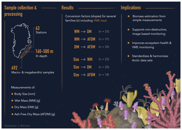
Conversion factors for Greenland shelf benthos: Weight-to-weight and body-size-to-weight relationships

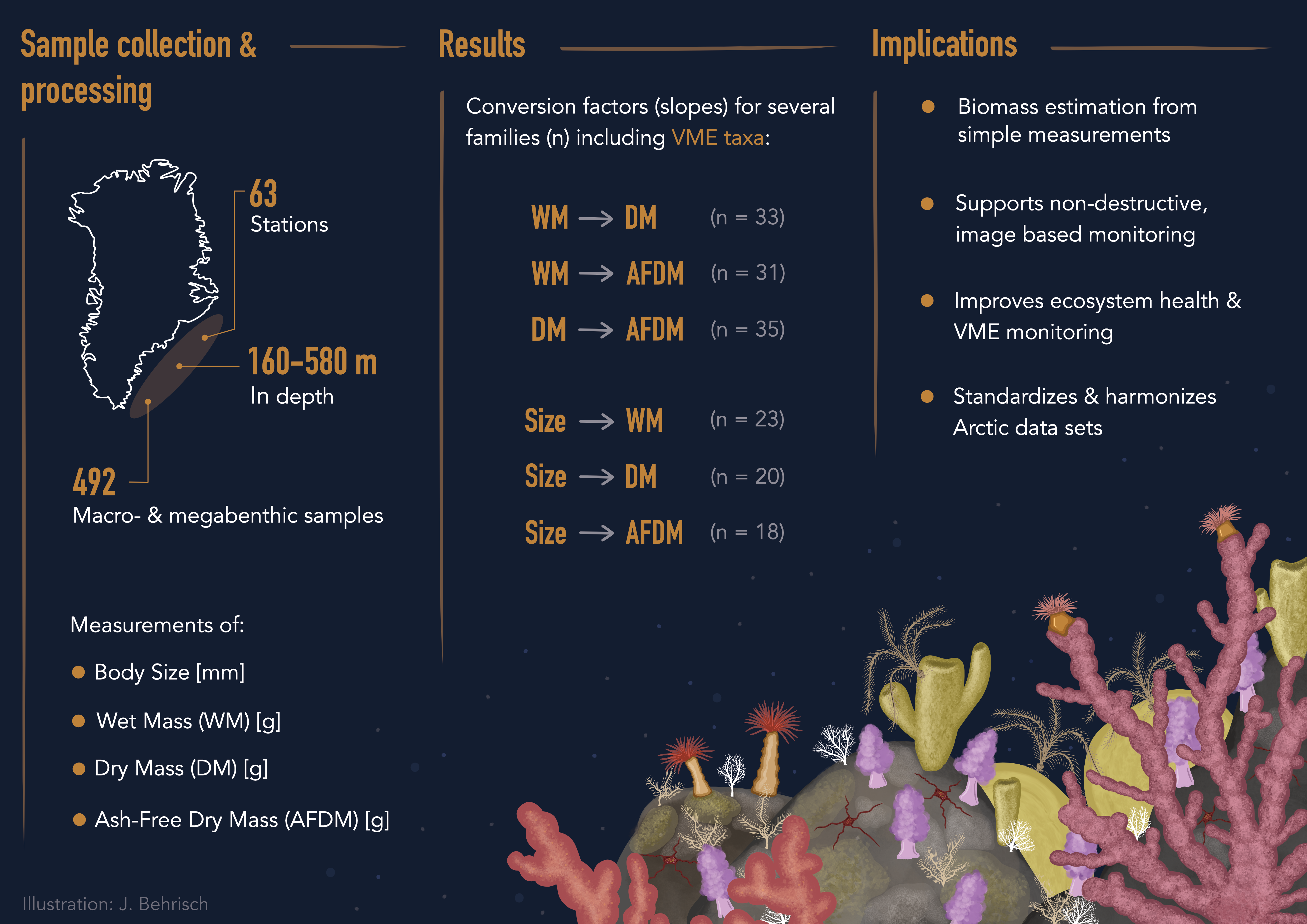
Climate change, biodiversity loss and increasing human activity are rapidly transforming Arctic marine ecosystems. Benthic ecosystems on Arctic shelves are important for biodiversity and ecosystem functioning. Biomass in the form of ash-free dry mass (AFDM) is often used as a proxy of ecosystem health but can be labour intensive and costly to obtain. This study addresses a key data gap by providing robust weight-to-weight and body-size-to-weight conversion factors for Arctic and boreal benthic fauna. We collected samples of common macro- and mega-benthic organisms in SE Greenland (59–67° N and 27–41° W) and calculated conversion factors (slopes) based on the relationship between wet mass (WM) to dry mass (DM) (33 families), WM to AFDM (31 families) and DM to AFDM (35 families) (https://doi.org/10.5281/zenodo.19346004, Behrisch and Zwerschke, 2026). To improve sampling output from non-destructive image-based sampling we also calculated conversion factors between body-size (length, diameter) and weight for a subset of families (Behrisch and Zwerschke, 2026). Our dataset includes several Vulnerable Marine Ecosystem (VME) indicator taxa for the Arctic region. The conversion factors for Atlantic-Arctic benthos presented here can serve as the foundation for a growing database, helping to unify datasets collected using different methodologies.

1 Introduction

Climate change, biodiversity loss and increasing human activity are rapidly reshaping polar marine ecosystems, particularly in the Arctic, where warming occurs at nearly four times the global average rate (Pörtner et al., 2024; Rantanen et al., 2022; Rigét et al., 2019). Arctic shelf benthos, including habitat-forming species such as sponges, soft corals, bryozoans, and hydroids, provide essential ecosystem services and can transform habitats into biodiversity and blue carbon hotspots (Buhl-Mortensen et al., 2010; Grebmeier et al., 2015; Souster et al., 2024). With the exception of some locations, such as the Barents Sea and regions in Canada, Arctic benthic ecosystems remain largely unmapped (CAFF, 2017; Jørgensen et al., 2015). Commonly, benthic bycatch monitoring programmes in the Arctic only record taxa wet mass, whilst more dedicated scientific studies often report ash-free dry mass (AFDM) as a more standardized measure of biomass (Jørgensen et al., 2015; Zwerschke et al., 2025). This is hampering efforts to combine datasets and assess the vulnerability of benthic Arctic communities to climate change and human activity across larger scales (CAFF, 2017).

Table 1 Sampling station information, including station number, mean depth [m], mean bottom temperature [°C], latitude and longitude per station. Depth and bottom temperature were derived from the Furuno Marport sensor attached to the trawl.

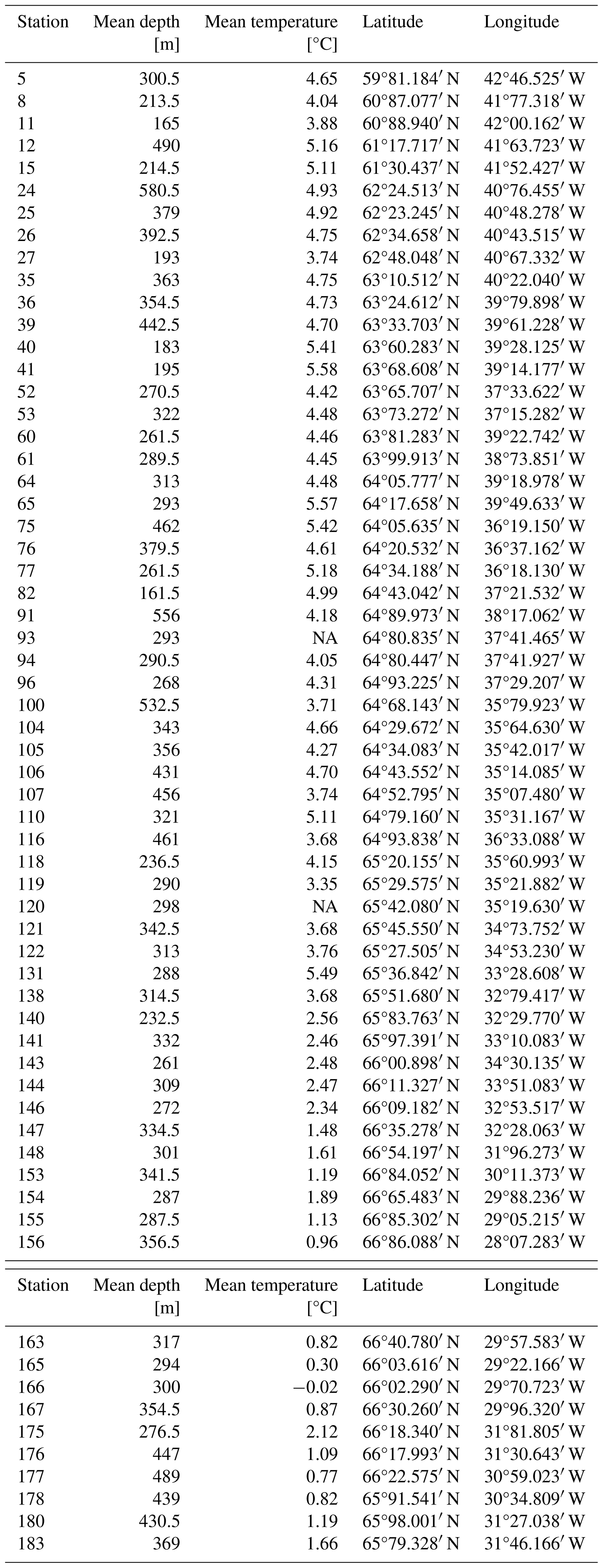
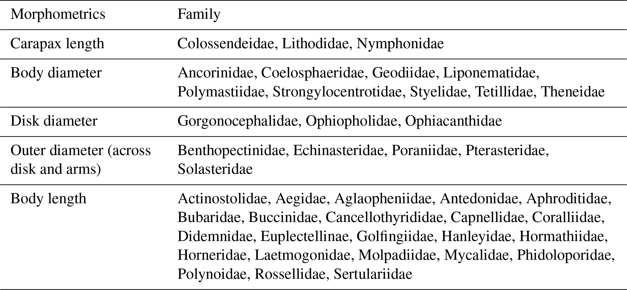
Table 2 Morphometrics indicating which body part was measured as a proxy for individual size (illustrated in Fig. S1).

Biomass within a community is often used as an indicator of ecosystem health. Changes in biomass can reflect changes in the abiotic environment, potentially caused by climate change (Hewitt et al., 2005; Rombouts et al., 2013; Sherman, 1994). Commonly, biomass is measured as ash-free dry mass (AFDM). It quantifies the organic material in a sample, excluding water and inorganic components found in the wet mass of organisms (Rumohr et al., 1987). The acquisition of AFDM is time and energy intensive, and, considering more novel and less invasive image-based analysis, often unobtainable. Image-based analysis often relies on abundance as a way to estimate community composition and change. This may bias the perceived importance of specific taxa within an ecosystem. For example, biomass and thus relevance within the ecosystem of few habitat forming taxa such as corals or sponges could easily outweigh those of a highly abundant species, such as spiroid worms (Kornder et al., 2021; Marlow et al., 2024).

Weight-to-weight or body-size-to-weight conversion factors provide a cost-effective alternative, allowing wet mass or body-size measurements to be converted to AFDM. This reduces the need for additional sampling, enables the harmonisation across datasets and supports non-destructive, image-based assessments (Javed and Hamid, 2025; Marlow et al., 2024). In the last three decades, weight-to-weight conversion factors have been calculated for various benthic macro-invertebrates across several global regions (Brey et al., 2010; Gogina et al., 2020, 2022; Lappalainen and Kangas, 1975; Petersen and Curtis, 1980; Ricciardi and Bourget, 1998; Rumohr et al., 1987; Stratmann et al., 2020; Tumbiolo and Downing, 1994). However, data on weight-to-weight and body-size-to-weight conversion factors remain scarce for most abundant boreal and Arctic benthic taxa. In particular, only limited literature exists on body-size-to-weight conversion factors for benthos (Eklöf et al., 2016). This gap is especially pronounced in regions such as Greenland, where knowledge of species distribution and ecosystem roles is limited. The ecological value of data derived from image analysis could be substantially enhanced by incorporating biomass estimates based on size-to-weight conversion relationships (Marlow et al., 2024). Expanding the use and availability of these approaches will further support the prioritisation of non-destructive sampling methods in the future.

Table 3 Wet mass (WM) [g] to dry mass (DM) [g] conversion factors (slopes) for 43 macro- and mega-benthic families. For each family, the column “n” indicates the total number of individuals used. The column “Confidence (C)” indicates the reliability of each slope using circles: $\circ =$ low, • = high. Confidence is based on sample size (n), R² and p-value from linear regressions or Spearman correlations: low → n < 5, R² < 0.7, p-values > 0.05; high → n ≥ 5, R² > 0.7, p-values < 0.05. Each slope of a family includes squared R values (R²) and 95 % confidence intervals (CI). The column “p” indicates the p-value from linear regression for each family; when assumptions were violated, Spearman rank correlation p-values are reported (underlined) (significance: ${}^{\ast \ast \ast }p$ < 0.001, ${}^{\ast \ast }p$ < 0.01, ^∗p < 0.05, ns – not significant). See Table S3 for more detail.

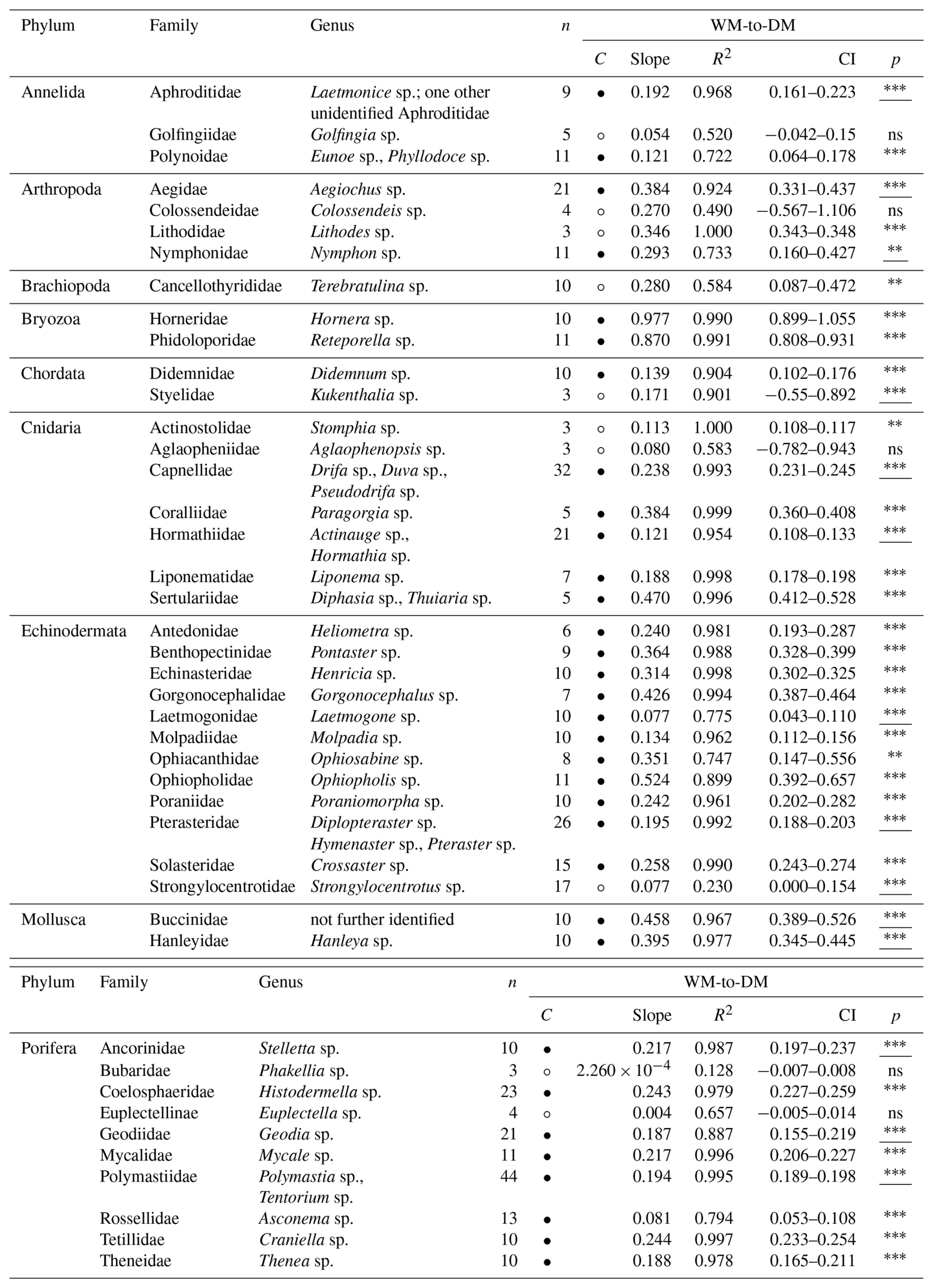
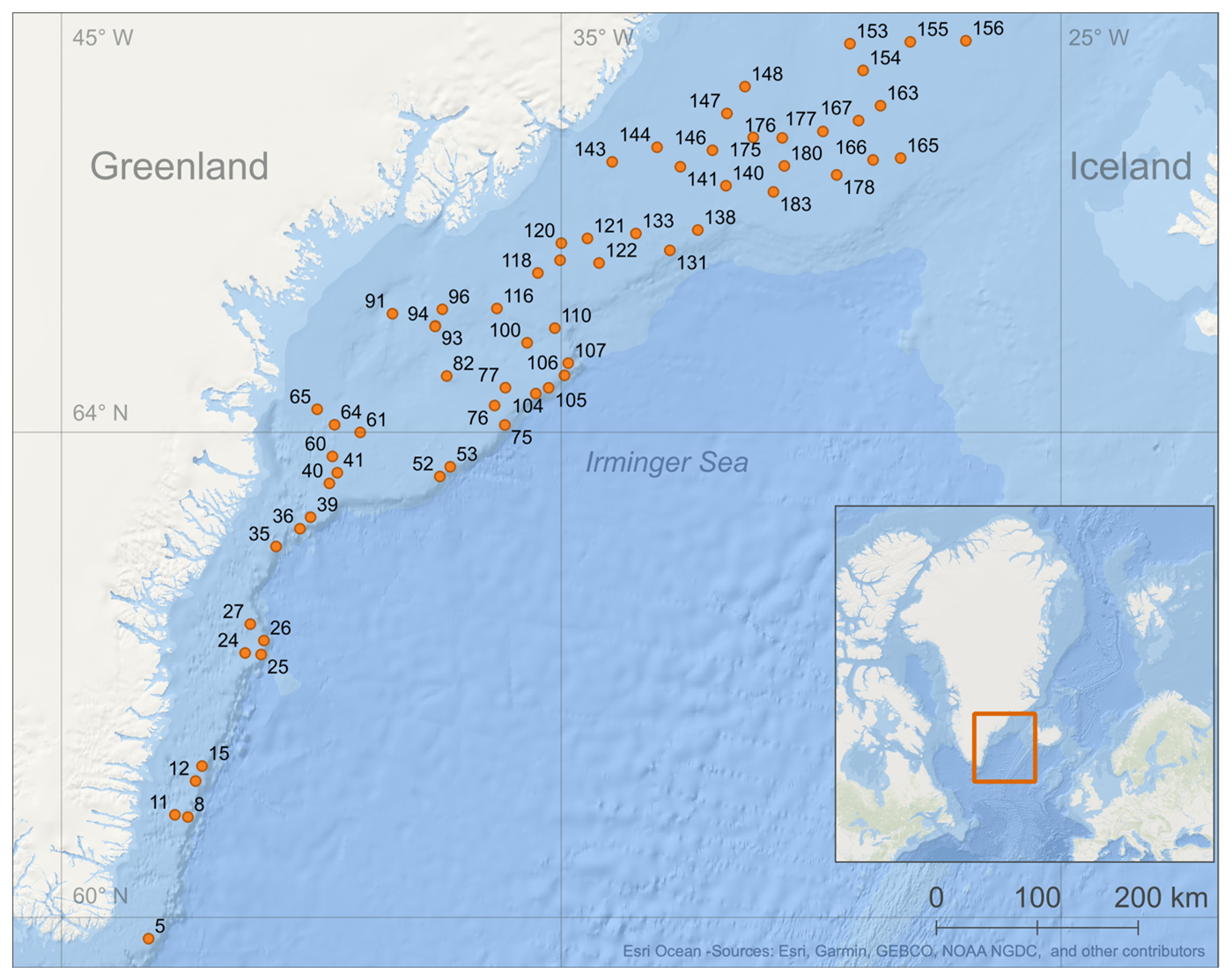
Figure 1 Map of the 63 stations (orange dots) with station numbers sampled during July and August 2023 along the East Greenland shelf (Basemap: Esri Ocean – Sources: Esri, Garmin, GEBCO, NOAA NGDC, and other contributors | Powered by Esri).

Table 4 Wet mass (WM) [g] and ash-free dry mass (AFDM) [g] conversion factors (slopes) for 43 macro- and mega-benthic families. For each family, the column “n” indicates the total number of individuals used. The column “Confidence (C)” indicates the reliability of each slope using circles: $\circ =$ low, • = high. Confidence is based on sample size (n), R² and p-value from linear regressions or Spearman correlations: low → n < 5, R² < 0.7, p-values > 0.05; high → n ≥ 5, R² > 0.7, p-values < 0.05. Each slope of a family includes squared R values (R² ) and 95 % confidence intervals (CI). The column “p” indicates the p-value from linear regression for each family; when assumptions were violated, Spearman rank correlation p-values are reported (underlined) (significance: ${}^{\ast \ast \ast }p$ < 0.001, ${}^{\ast \ast }p$ < 0.01, ^∗p < 0.05, ns – not significant). See Table S4 for more detail.

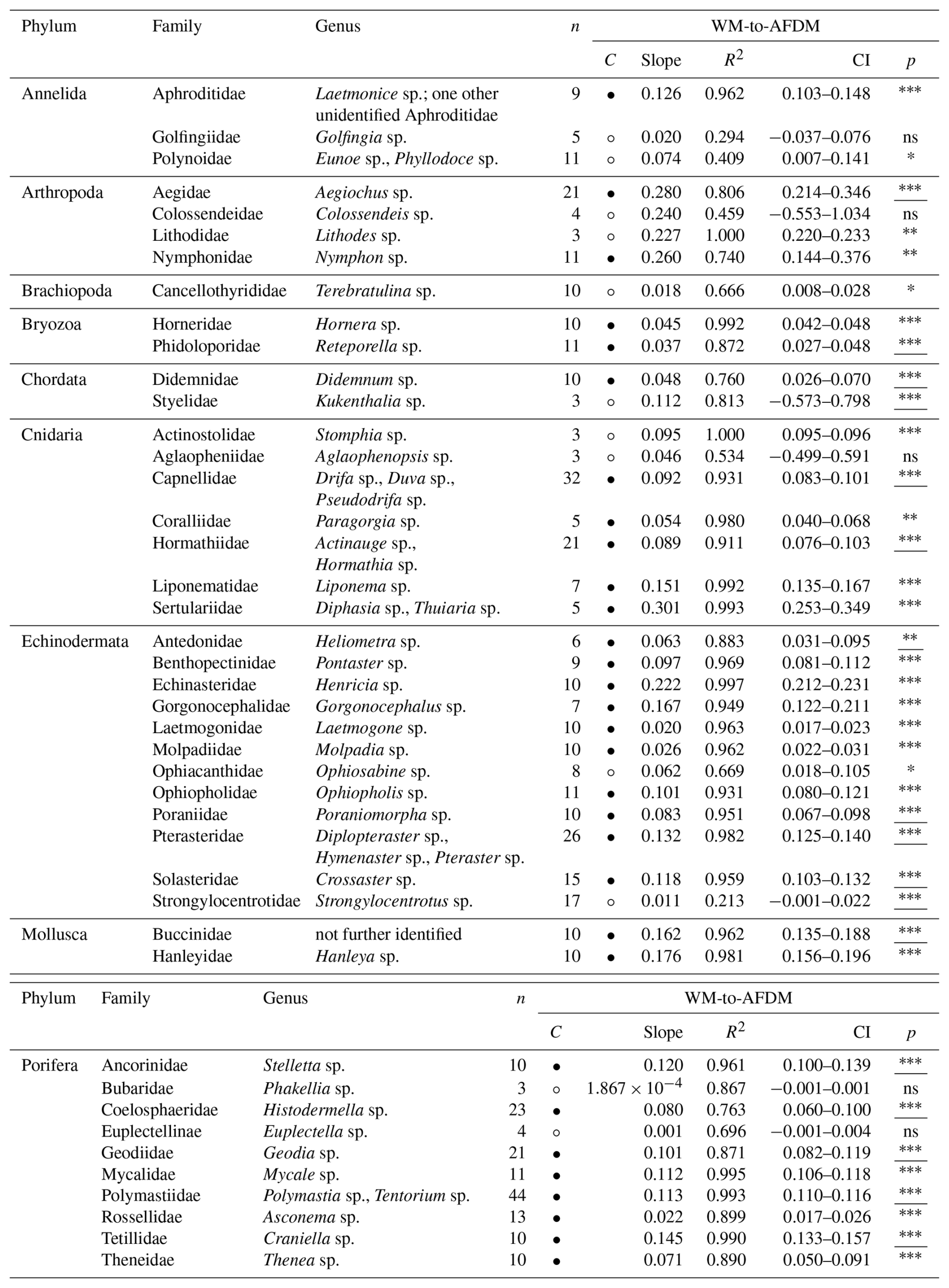
Table 5 Dry mass (DM) [g] and ash-free dry mass (AFDM) [g] conversion factors (slopes) for 43 macro- and mega-benthic families. For each family, the column “n” indicates the total number of individuals used. The column “Confidence (C)” indicates the reliability of each slope using circles: $\circ =$ low, $•=$ high. Confidence is based on sample size (n), R² and p-value from linear regressions or Spearman correlations: low → n < 5, R² < 0.7, p-values > 0.05; high → n ≥ 5, R² > 0.7, p-values < 0.05. Each slope of a family includes squared R values (R²) and 95 % confidence intervals (CI). The column “p” indicates the p-value from linear regression for each family; when assumptions were violated, Spearman rank correlation p-values are reported (underlined) (significance: ${}^{\ast \ast \ast }p$ < 0.001, ${}^{\ast \ast }p$ < 0.01, ^∗p < 0.05, ns – not significant). See Table S5 for more detail.

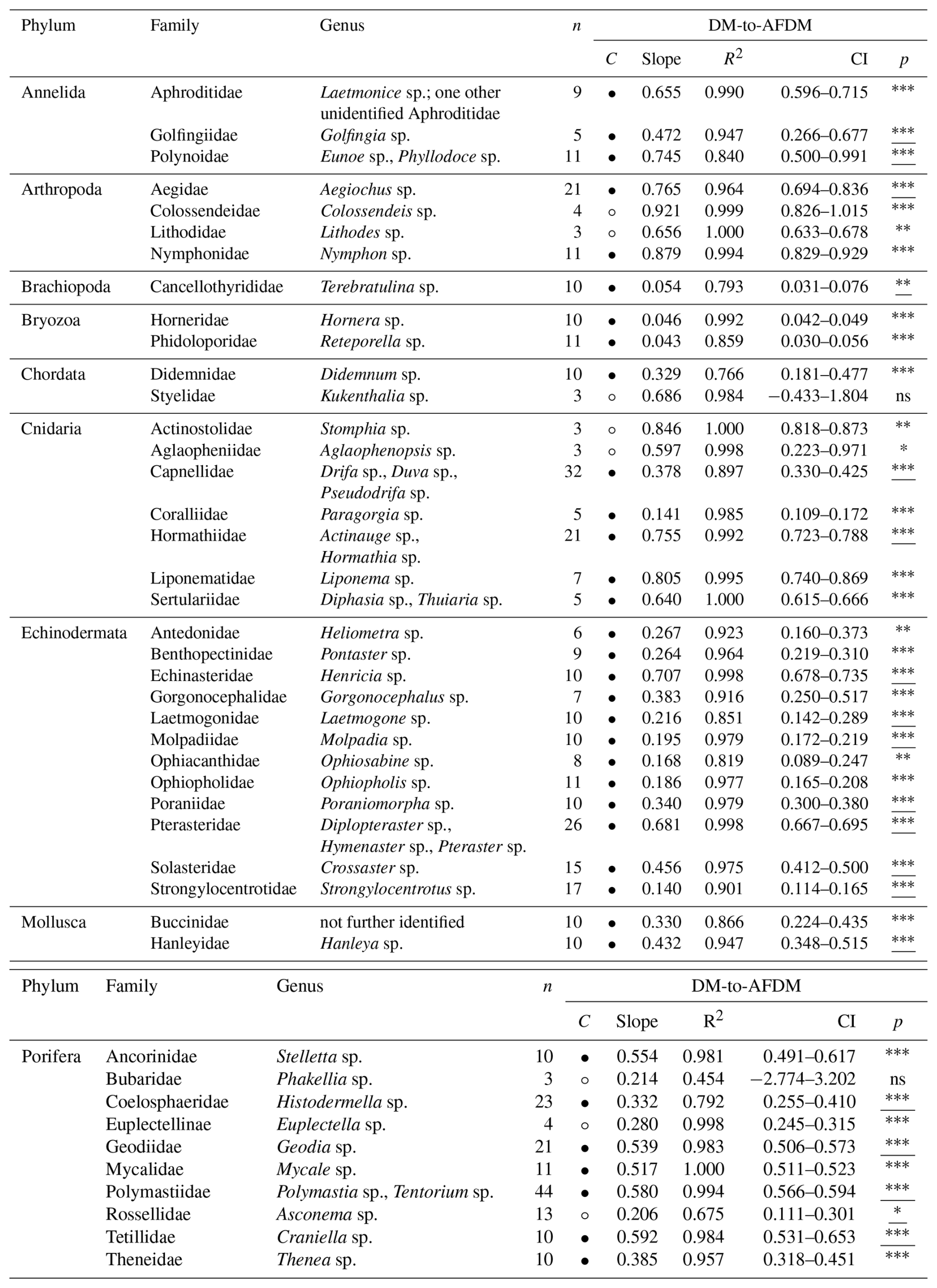
Table 6 Size [mm] and wet mass (WM) [g] conversion factors (slopes) for 43 macro- and mega-benthic families. For each family, the column “n” indicates the total number of individuals used. The column “morphometrics” indicates species-specific morphometric features measured to assess body size. The column “Confidence (C)” indicates the reliability of each slope using circles: $\circ =$ low, $•=$ high. Confidence is based on sample size (n), R² and p-value from linear regressions or Spearman correlations: low → n < 5, R² < 0.7, p-values > 0.05; high → n ≥ 5, R² > 0.7, p-values < 0.05. Each slope of a family includes squared R values (R²) and 95 % confidence intervals (CI). The column “p” indicates the p-value from linear regression for each family; when assumptions were violated, Spearman rank correlation p-values are reported (underlined) (significance: ${}^{\ast \ast \ast }p$ < 0.001, ${}^{\ast \ast }p$ < 0.01, ^∗p < 0.05, ns – not significant). See Table S6 for more detail.

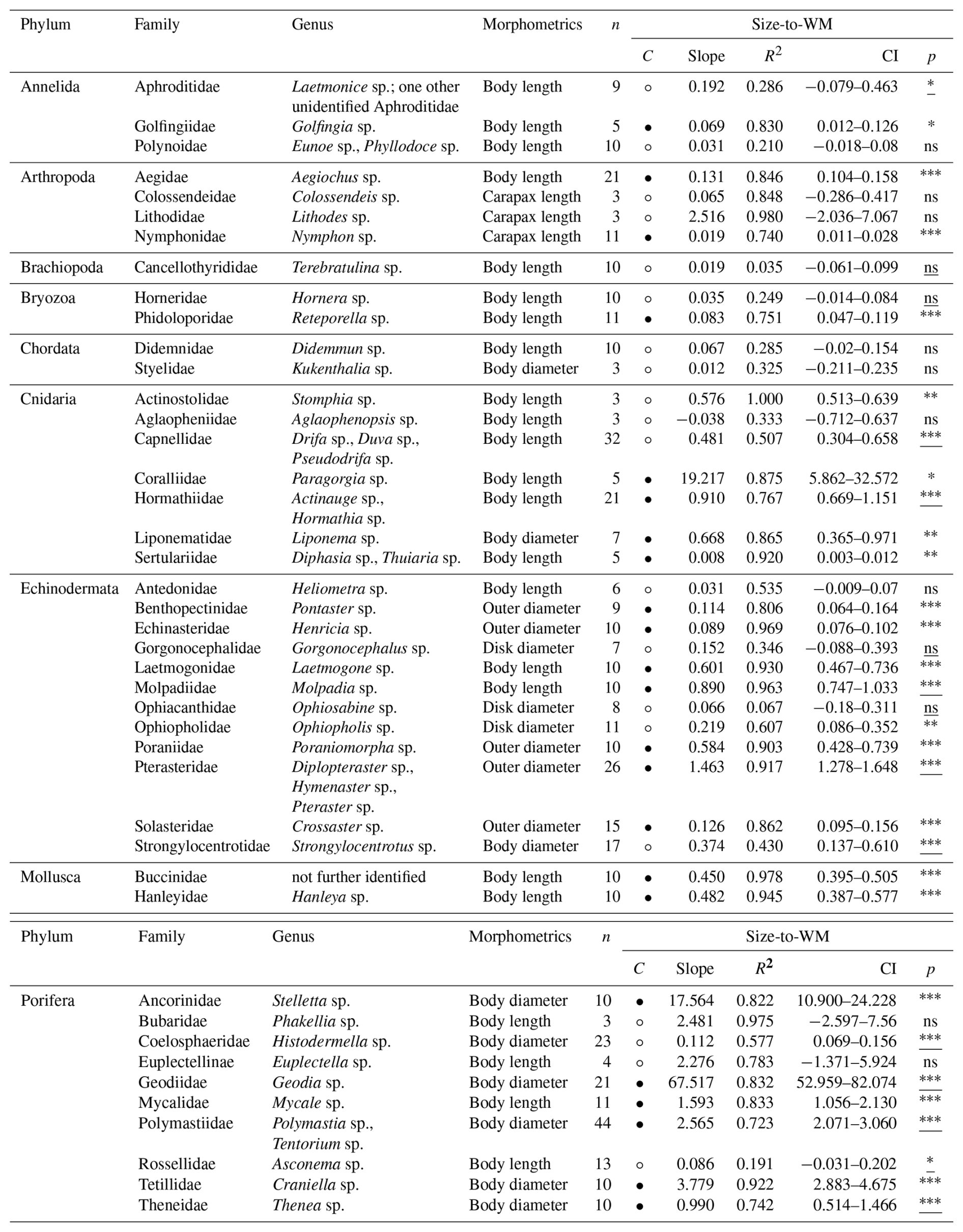
Table 7 Size [mm] and dry mass (DM) [g] conversion factors (slopes) for 43 macro- and mega-benthic families. For each family, the column “n” indicates the total number of individuals used. The column “morphometrics” indicates species-specific morphometric features measured to assess body size. The column “Confidence (C)” indicates the reliability of each slope using circles: $\circ =$ low, $•=$ high. Confidence is based on sample size (n), R² and p-value from linear regressions or Spearman correlations: low → n < 5, R² < 0.7, p-values > 0.05; high → n ≥ 5, R² > 0.7, p-values < 0.05. Each slope of a family includes squared R values (R²) and 95 % confidence intervals (CI). The column “p” indicates the p-value from linear regression for each family; when assumptions were violated, Spearman rank correlation p-values are reported (underlined) (significance: ${}^{\ast \ast \ast }p$ < 0.001, ${}^{\ast \ast }p$ < 0.01, ^∗p < 0.05, ns – not significant). See Table S7 for more detail.

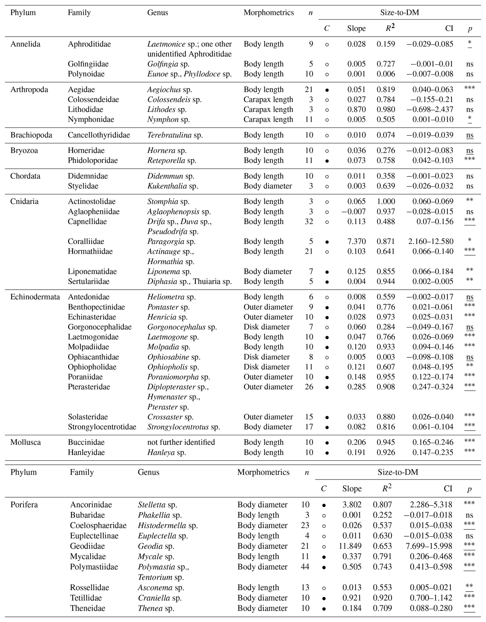
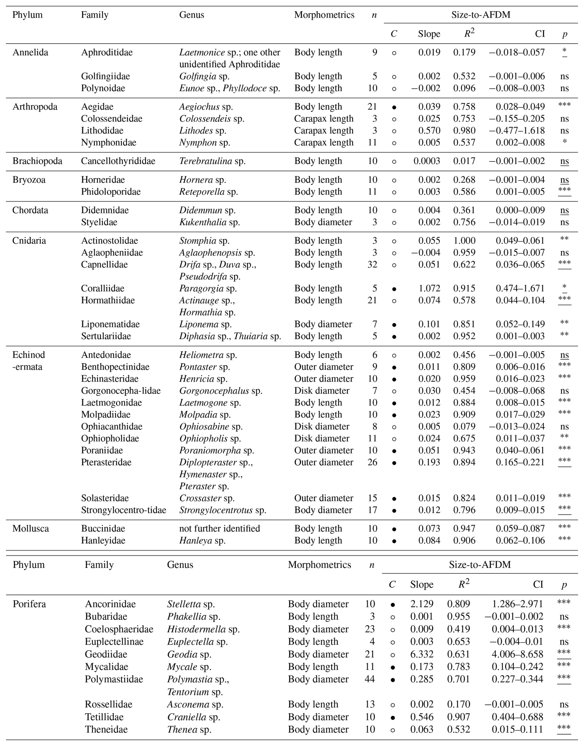
Table 8 Size [mm] and ash-free dry mass (AFDM) [g] conversion factors (slopes) for 43 macro- and mega-benthic families. For each family, the column “n” indicates the total number of individuals used. The column “morphometrics” indicates species-specific morphometric features measured to assess body size. The column “Confidence (C)” indicates the reliability of each slope using circles: $\circ =$ low, $•=$ high. Confidence is based on sample size (n), R² and p-value from linear regressions or Spearman correlations: low → n < 5, R² < 0.7, p-values > 0.05; high → n ≥ 5, R² > 0.7, p-values < 0.05. Each slope of a family includes squared R values (R²) and 95 % confidence intervals (CI). The column “p” indicates the p-value from linear regression for each family; when assumptions were violated, Spearman rank correlation p-values are reported (underlined) (significance: ${}^{\ast \ast \ast }p$ < 0.001, ${}^{\ast \ast }p$ < 0.01, ^∗p < 0.05, ns – not significant). See Table S8 for more detail.

Our study provides reliable conversion factors (slopes) based on the linear relationship between WM-to-DM, WM-to-AFDM, and DM-to-AFDM, as well as body-size-to-WM, body-size-to-DM, and body-size-to-AFDM and their associated confidence level. These cover common macro- and mega-benthic families along the East Greenland Shelf, including several VME indicator taxa from the FAO VME indicator list for the Northeast Atlantic (FAO, 2025). A comprehensive database for Arctic benthic conversion factors does not yet exist, and the data presented here, is a first step towards providing reliable conversion factors for international monitoring and management efforts (e.g. Circumpolar Biodiversity Monitoring Program (CBMP), State of the Arctic marine biodiversity report (SAMBR)). This can be built on, by other projects and monitoring programmes and, may eventually, be included into other international databases such as the Arctic Traits database (Degen and Faulwetter, 2019).

2 Materials and Methods

2.1 Sampling location

Benthic macro- and mega-invertebrate samples were collected as part of a trawl-bycatch programme at the Greenland Institute of Natural Resources (GINR) (Zwerschke et al., 2025) from 11 July to 2 August 2023 on the research vessel Tarajoq between SE Greenland and the Tasiilaq region (59–67° N and 27–41° W). Sampling took place at 63 stations, including the shelf edge and shelf slope, as well as glacial troughs and banks, spanning depths between 160 and 580 m (Fig. 1 and Table 1).

2.2 Sampling procedures and processing

2.2.1 Benthic sample collection with cosmos trawl

At each station a cosmos bottom trawl (twin-body trawl) was deployed and towed for 15 min. The trawl consisted of a funnel section, splitting into two extension sections and two codends. The funnel section and extension sections had a mesh size of ∼ 4.45 cm. The net was held open by two heavy otter doors and the mouth of the open net had a size of approximately 1.14 m (side) × 3 m (headline). The station start and end location was recorded and temperature [°C], as well as depth [m], were recorded every 2 min based on the readings of a MARPORT Trawl Explorer Pro^® sensor. Benthic fauna from each trawl were identified to the lowest possible taxonomic resolution based on morphology. Identification was supported by unpublished material developed by regional taxonomic experts, as well as by available identification guides from adjacent regions and literature on specific taxonomic groups (Best et al., 2010; Blicher et al., 2015; Grant et al., 2018; Kenchington et al., 2015; Nozères et al., 2014). Nomenclature was updated to the most recent accepted term via the World Register of Marine Species (WoRMS Editorial Board, 2025). Most samples were identified to the genus level. However, some could only be identified to family level. Samples were processed fresh whenever possible. If immediate processing was not feasible, they were stored at −20 °C until further processing.

Sampling aimed to obtain representatives of each family across the full spatial range of stations. However, stations differed in depth, shelf habitat (trough, banks, shelf edge), and latitude/longitude, which can influence family abundances and community composition (Blicher and Arboe, 2021; Carney, 2005; Curtis, 1975; Levin et al., 2001). For conversion factors, sampling targeted 10 individuals per benthic family, prioritizing taxa that serve as VME indicators or were dominant components of the habitat (e.g., high density in the catch). Despite this, natural variability meant some families were rare or only abundant at a single station, resulting in either low overall sample sizes or high sample numbers concentrated at one station. Conversion factors were calculated using all available individuals of a family, regardless of station or environmental context. Consequently, these values may not reflect spatial variability.

For each taxon, we included a balanced variety of body sizes and morphologies and avoided targeting specific body sizes or inclusion of atypical morphologies, such as disproportionately large shells or spicules. Fragile habitat-dominating species (such as bryozoans, like Hornera lichenoides or the glass sponge, Asconema sp.), often obtained as fragments, were still included in sample collection due to their ecological importance and frequent occurrence. The size and biomass of each fragment were measured and processed in the same way as for complete organisms, with conversion factors derived from the fragment measurements rather than from whole organisms. External, internal and skeletal structures, such as bivalve shells and echinoderm tests, were included in the weight measurements. Individuals that were heavy (> 100 g) or large (e.g., round sponges of the genera Craniella sp. and Geodia sp.) were sub-sampled. To obtain reliable subsamples, a cross-section containing a variety of different tissues from an individual was taken. All full samples, fragments and subsamples were stored in a −20 °C freezer until further processing in the laboratory.

2.2.2 Assessing the body size, WM, DM and AFDM

In the laboratory, the wet mass (WM) [g] of each full individual was measured as blotted wet weight. Echinoderms were weighed without piercing or draining and were processed in the same manner as other taxa. Wet mass measurements were conducted onboard using a fine scale (accuracy of ±0.0001 g). In addition, the body size [mm] of the full individual was measured using species specific morphometric features with calipers (mm) (Table 2, Fig. S1 in the Supplement). Individuals were not anaesthetized prior to measurement of body size and wet mass, as they were often immobile at the time of sampling. Afterwards, samples were dried at 70 °C for at least 48 h or until a constant dry mass (DM) [g] was reached and subsequently burned at 450 °C for 24 h. Dry mass and ash mass (AM) [g] were measured using an analytical balance with an accuracy of ±0.0001 g. Ash mass was subtracted from DM to calculate the AFDM [g] of a sample. For subsamples, AFDM was extrapolated based on the total WM of the full sample.

2.3 Statistical Analyses

Analyses were performed at the family level to ensure sufficient sample sizes (n ≥ 3). We aimed to calculate conversion factors (slopes) between different biomass measures (WM, DM, AFDM) and between body size and biomass for each taxonomic family. For this, we calculated the slope (s) of linear regressions with WM, DM, and AFDM as response variables and either another biomass measure or body size as the predictor. Residuals were used to assess whether data fitted the assumptions of the model. Linearity was assessed visually using scatterplots and residuals versus fitted value plots. Normality of residuals was examined using Q-Q plots and the Shapiro–Wilk test (Shapiro and Wilk, 1965), and homoscedasticity was tested using the Breusch-Pagan test (Breusch and Pagan, 1979) with the R package “car” (Tables S1–S2) (R Core Team, 2022). For families that did not meet linear regression assumptions, slopes were calculated as above, while significance was evaluated using non-parametric Spearman rank correlations (Dodge, 2008; Glasser and Winter, 1961; Spearman, 1904). All statistical analyses were conducted in R version 2024.04.0+735 (R Core Team, 2022).

3 Results

A total of 492 samples were collected across 63 stations. All samples were used for weight-to-weight relationships, whereas two samples were excluded for body-size-to-weight relationships owing to lacking size measurements. In total, 43 benthic families were analyzed. These families include key VME indicator taxa such as feather stars (Antedonidae), cauliflower soft corals (Capnellidae), gorgonian soft corals (Coralliidae), demosponges (Ancorinidae, Geodiidae, Polymastiidae, Tetillidae, Theneidae), glass sponges (Euplectellinae, Rossellidae) and bryozoans (Horneridae, Phidoloporidae) (FAO, 2025). Numbers of individuals sampled per family varied from three to 44 across all stations (Fig. S2). Overall, we identified 33 (WM–DM), 31 (WM–AFDM), and 35 (DM–AFDM) reliable linear relationships for biomass conversions (Tables 3–5, Figs. S3–S5) and 23 (size-to-WM), 20 (size-to-DM), and 18 (size-to-AFDM) reliable linear relationships for size-to-biomass conversions (Tables 6–8, Figs. S6–S8). Reliable linear relationships were identified as those with sample size n ≥ 5, R²> 0.7 and p< 0.05 (Tables 3–8) (Behrisch and Zwerschke, 2026). For several families, regression models explained a substantial proportion of the variance (R² > 0.5), without being statistically significant. This is caused by low sample size (e.g. Actinostolidae WM–AFDM: R²= 1, n = 3). In addition to Actinostolidae (sea anemones), weight-to-weight and body-size-to-weight relationships of the families Aglaopheniidae (hydroids), Bubaridae (demosponges), Lithodidae (king crabs), and Styelidae (tunicates) were also calculated from only three samples and should be interpreted with caution. We have chosen to still report these values albeit indicating low confidence in their accuracy. This way future work can build upon the data made available here.

Weight-to-weight and body-size-to-mass relationships varied widely across taxa and mass types. Overall, the steepness of each weight-to-weight slope was determined by the fraction of water, inorganic structural material, and metabolically active, organic tissue contained in an organism. Taxa with high water or organic content lose proportionally more mass during drying or ashing, resulting in shallower slopes, whereas taxa dominated by inorganic tissue retain more mass, producing steeper slopes (Figs. S3–S5). Regarding body-size-to-biomass relationships, shallow slopes were generally observed across all mass types in smaller organisms with low proportions of organic tissue, where increases in body size correspond to only minor increases in DM, AFDM, or WM. Steeper slopes occur in larger organisms with a mix of organic and inorganic tissue, substantial metabolically active tissue or structural/inorganic components, reflecting greater overall mass accumulation (Figs. S6–S8). These patterns highlight the need for taxon-specific slopes when estimating biomass from weight-to-weight and body-size-to-weight relationships.

3.1 Weight-to-weight relationships

Reliable WM-to-DM relationships demonstrate that WM is a good predictor of DM in these cases (Table 3). Slopes between WM and DM varied widely across taxa, with shallower slopes for Porifera (Bubaridae: s= 2.26×10⁴), yet very steep slopes for Bryozoa (Horneridae: s= 0.977) (Table 3). Shallower slopes (s< 0.15) were generally associated with soft-bodied taxa, that contained higher water content, like anemones (Cnidaria: Hexacorallia), sea cucumbers (Echinodermata: Holothuroidea), and glass sponges (Porifera: Hexactinellida). Steeper slopes (s > 0.3) were associated with taxa which feature greater portions of inorganic material (Arthropoda, Mollusca, Bryozoa, demosponges and gorgonian soft corals (Coralliidae)) (Fig. S3). Reliable WM-to-DM relationships could be calculated for the majority of sampled VME indicator taxa, such as bryozoans (Horneridae, Phidoloporidae), feather stars (Antedonidae), cauliflower soft corals (Capnellidae), gorgonian soft corals (Coralliidae), demosponges (Ancorinidae, Geodiidae, Polymastiidae, Tetillidae, Theneidae), and glass sponges (Rossellidae) (FAO, 2025).

Slopes between WM and AFDM also varied widely across taxa, ranging from very shallow ($s=\mathrm{1.867}\times {\mathrm{10}}^{\mathrm{4}}$ in Porifera : Bubaridae) to steeper values (s=0.301 in Cnidaria : Sertulariidae) (Table 4). The shallowest slopes (s< 0.05) were mainly associated with Porifera and some Echinodermata, like sea cucumbers (Holothuroidea) (Fig. S4). This may be caused by high water content in the wet tissues (sea cucumbers) and a greater ratio of inorganic to organic matter within the organisms. Steeper slopes (s > 0.15) were typical of Arthropoda and Mollusca, consistent with their greater metabolically active tissue. Reliable WM-to-AFDM relationships could be calculated for the same 11 VME indicator taxa as for WM-to-DM relationships (FAO, 2025).

Slopes for DM-to-AFDM ranged from 0.043 in Bryozoa (Phidoloporidae) to 0.921 in Arthropoda (Colossendeidae) (Table 5). Shallow slopes (s<0.3) were generally observed in taxa with a high proportion of structural or inorganic material relative to organic tissue, including Porifera, Brachiopoda, Bryozoa, and some Echinodermata and Cnidaria (Fig. S5). Moderate slopes (s= 0.3–0.6) were associated with taxa with a similar ratio of inorganic to organic matter (Echinodermata, Cnidaria, Mollusca, Chordata). Steep slopes (s > 0.6) were found in taxa with high content of metabolically active, organic tissue, including Arthropoda, Annelida, and soft-tissue Cnidaria, where most dry mass is retained as AFDM. Reliable DM-to-AFDM relationships could be calculated for 10 VME indicator taxa, such as bryozoans (Horneridae, Phidoloporidae), feather stars (Antedonidae), cauliflower soft corals (Capnellidae), gorgonian soft corals (Coralliidae), and demosponges (Ancorinidae, Geodiidae, Polymastiidae, Tetillidae, Theneidae) (FAO, 2025).

3.2 Body-size-to-weight relationships

For two families, size-to-biomass relations were negative (size to WM, DM and AFDM for Aglaopheniidae; size to AFDM for Polynoidae) (Tables 6–8, Figs. S6–S8). For these taxa, correlation tests indicated no significant relationship (p-value > 0.05) between body size and biomass. It is possible that alternative size metrics (e.g. width) would yield more meaningful relationships. However, based on the current results, these taxa are not suitable candidates for body-size-to-weight conversions.

For body-size-to-WM, slopes ranged from very shallow (hydrozoans, e.g. Sertulariidae with 0.008) to very steep in large-bodied Porifera and Cnidaria (e.g., Porifera : Geodiidae, 67.517; Cnidaria : Paragorgia sp., 19.217) (Table 6). Shallow slopes (s<0.09) were generally associated with small-bodied taxa, including hydrozoans, bryozoans, sea spiders, and polychaetes. Organisms with greater tissue mass and higher water content, such as anemones (Cnidaria : Hexacorallia), sea cucumbers (Echinodermata : Holothuroidea), and molluscs, showed intermediate increases ($\mathrm{0.1}<s<\mathrm{1}$) in wet mass with size. Large-sized demosponges (Ancorinidae, Geodiidae) and gorgonian corals (Coralliidae), with high tissue and structural mass, showed strong increases in wet mass with increasing size (s≥2) (Fig. S6). Reliable size-to-WM relationships could be calculated for seven VME indicator taxa: bryozoans (Phidoloporidae), gorgonian soft corals (Coralliidae), and demosponges (Ancorinidae, Geodiidae, Polymastiidae, Tetillidae, Theneidae) (FAO, 2025).

Body-size-to-DM slopes ranged from 0.001 (Annelida : Polynoidae; Porifera : Bubaridae) to 11.849 (Porifera : Geodiidae) (Table 7). Shallow slopes (s<0.08) were observed in small-bodied annelids, bryozoans, and hydrozoans, which showed relatively limited increases in organic and inorganic mass with increasing body size. Steeper slopes (s> 3) were associated with large-bodied demosponges (Ancorinidae, Geodiidae) and gorgonian corals (Coralliidae), which showed strong increases in skeletal and organic structural material with size (Fig. S7). Reliable size-to-DM relationships could be calculated for six VME indicator taxa: bryozoans (Phidoloporidae), gorgonian soft corals (Coralliidae), and demosponges (Ancorinidae, Polymastiidae, Tetillidae, Theneidae) (FAO, 2025).

Body-size-to-AFDM slopes ranged from near zero (e.g., Brachiopoda: Cancellothyrididae with s= 0.0003) to 6.332 in Porifera (Geodiidae) (Table 8). Small-bodied taxa with relatively low organic content, such as annelids, brachiopods, cnidarians, and echinoderms, showed shallower slopes (s< 0.1). Steeper slopes (s> 1) were found in large-bodied sponges (Porifera) and gorgonian corals (Coralliidae), which showed strong increases in metabolically active organic tissue with body size (Fig. S8). Reliable size-to-AFDM relationships included four VME indicator taxa: gorgonian soft corals (Coralliidae), and demosponges (Ancorinidae, Polymastiidae, Tetillidae) (FAO, 2025).

The definition of what constitutes a reliable conversion factor was quite stringent for size to weight relationships, which naturally incorporate some more variation in terms of environmental factors shaping morphology (e.g. more stunted growth in high velocity environments) (Chamberlain Jr. and Graus, 1975). As a result, some well-sampled taxa (e.g. Geodia sp.) exhibited significant biomass-size relationships but were not classified as reliable due to moderate explanatory power (e.g. R² = 0.63–0.65) (Tables 7 and 8). Significant relationships with higher residual variation, may, however, still be useful in further analyses if this uncertainty is explicitly accounted for.

Overall, several factors could explain the lack of a significant linear relationship between body mass metrics, as well as body size and body mass. For families like Strongylocentrotidae, for example, gonad production or recent feeding events, constitute a major component of their body mass, potentially distorting any size to weight relationships (Blicher et al., 2007). Furthermore, sea cucumbers (Echinodermata: Holothuroidea) can expel their internal organs (evisceration) as a defense strategy. Though strategies vary across sea cucumbers (Emson and Wilkie, 1980; García-Arrarás and Greenberg, 2002; Hyman, 1955), the genera Laetmogone sp. and Molpadia sp. may use this defense during the sampling event, which could impact biomass estimates in the present study. Non-linear and colonial growth patterns, such as found in some sponges, hydroids and bryozoans, can limit the use of size for specific taxa as a biomass indicator. Additionally, for some delicate, fragile taxa (such as feather stars (Antedonidae) or sponges of the family Bubaridae and Rossellidae), it was impossible to collect the entire specimen. This may have limited which parameters could be measured (e.g. only size/weight of the calyx of the crinoids could be measured rather than the total animal) and could have introduced a certain degree of bias in the results.

In general, results indicate that taxa with stable and structurally robust body plans and consistent tissue composition, particularly demosponges, echinoderms, molluscs, cnidarians and arthropods, are well suited for deriving reliable weight-to-weight and body-size-to-weight relationships.

4 Data availability

All raw measurement data, primary result tables (slopes, i.e., conversion factors), and R scripts used for data processing and analyses are available in the open repository Zenodo (https://doi.org/10.5281/zenodo.19346004, Behrisch and Zwerschke, 2026). All quality-checked measurements are included without selective exclusion. The tables in the Supplement, which include the Spearman rank correlation test results, are provided in the publication (Tables S3–S4).

5 Conclusion

This study provides robust weight-to-weight conversion factors and body-size-to-weight conversion factors (i.e., conversion slopes) for some of the most dominant boreal and Arctic shelf megafauna, including critical Vulnerable Marine Ecosystem (VME) taxa, for the first time. We demonstrate that WM is a reliable predictor of DM and AFDM for most families in this study. In addition, we establish robust relationships between body size and biomass, showing that body size can serve as a reliable proxy for WM, DM, and AFDM in several benthic families. Together, these conversion factors strengthen the potential for non-destructive sampling approaches, including image-based surveys, allowing ecosystem assessments while minimizing disturbance to sensitive habitats. Additionally, it will guide future efforts in estimating conversion factors by indicating, families that have not been sufficiently sampled yet. This dataset provides a baseline, which can be repeatedly updated and to which further existing data can be added to improve the taxonomic resolution and its usefulness for future work. By providing a baseline dataset, this study enables harmonisation of different datasets across the Arctic for specific common taxa (e.g., Geodia sp.). This allows for a more comprehensive estimation of ecosystem health and monitoring of VME indicator taxa (Zwerschke et al., 2025). As pressures on scientific resources increase and the ethics of destructive sampling of the few remaining pristine habitats are more and more questionable, datasets like these will help to streamline and improve future sampling and monitoring events in the Arctic, enhancing our capacity to assess and manage these vulnerable marine communities (Javed and Hamid, 2025; Marlow et al., 2024).