Hydrologic, biogeochemical, microbial, and macroinvertebrate responses to network expansion, contraction, and disconnection across headwater stream networks with distinct physiography in Alabama, USA

Here we present a comprehensive dataset of hydrologic, biogeochemical, microbial, and macroinvertebrate community measurements from a set of multi-year, co-occurring, watershed studies in non-perennial stream networks that dynamically expand and contract over space and time. The data were collected over the three consecutive water years (Autumn 2021–Autumn 2024) across three stream networks draining watersheds with a similar humid, subtropical climate but distinct physiographies (i.e., Piedmont, Appalachian Plateau, Coastal Plain) in Alabama, USA. Our goal was to characterize the spatiotemporal patterns and drivers of how non-perennial stream networks expand and contract, as well as the biogeochemical, microbial, and macroinvertebrate dynamics associated with changes in network connectivity and water availability. We used a combination of spatial, temporal, and spatiotemporal sampling and sensor-based monitoring approaches to capture hydrologic, biogeochemical, and ecological responses to network expansion and contraction in each watershed. This manuscript describes the overall study design, monitoring network and sampling approaches, data and sample collection and analysis, and specific datasets generated. All data products are publicly available through the “Aquatic Intermittency effects on Microbiomes in Streams” (AIMS) Hydroshare data repository for hydrologic, biogeochemical, and macroinvertebrate data (AIMS region code = “SE”; https://www.hydroshare.org/group/247, Plont et al., 2026t) and through the NCBI data repository for microbial data. All data product-specific DOIs and repository-specific unique IDs are cited in Appendix A (Tables A1, A3).

1 Introduction

Non-perennial streams, or streams that cease flowing throughout the year (also known as intermittent rivers and ephemeral streams, IRES; Busch et al., 2020), are ubiquitous, making up over half of global stream miles (Messager et al., 2021). Despite their ephemeral connectivity to permanent water bodies, non-perennial streams contribute over half of the streamflow on average to downstream river systems in the United States (Brinkerhoff et al., 2024), generate unique biogeochemical and ecological signals compared to perennial streams (Bernal et al., 2022; Gómez-Gener et al., 2021; López-Rojo et al., 2025; Zarek et al., 2025), and serve as important determinants of downstream water quality, biodiversity, and ecosystem services (Datry et al., 2023; Gómez et al., 2017; Marcé et al., 2019; Meyer et al., 2007). Climate change is altering the timing and severity of large storms and droughts, leading to unprecedented shifts in the geographic extent and hydrologic regimes of non-perennial streams (Tramblay et al., 2021; Zipper et al., 2021), highlighting the need to include these vulnerable ecosystems in policy and regulatory frameworks (Lane et al., 2023; Walsh and Ward, 2022). However, these systems remain largely absent from streamflow and water-quality monitoring networks (Krabbenhoft et al., 2022), hindering our ability to study downstream consequences of changing flow and connectivity dynamics in non-perennial streams. Given their variability and spatial complexity, we must also look upstream of the watershed outlet and utilize coordinated, interdisciplinary approaches to understand the patterns and drivers of network-scale connectivity, biogeochemistry, and ecology in non-perennial systems (Bernal et al., 2025; Zimmer et al., 2022). Further, watershed-scale studies on non-perennial streams are lacking in more mesic regions such as the southeastern USA (Krabbenhoft et al., 2022), which serves as a globally-important hotspot freshwater biodiversity (Meyer et al., 2007), and as a region is expected to undergo further climate-driven hydrologic intensification in the coming decades (Zipper et al., 2021).

Contextualizing the role of expansion, contraction, and intermittency in freshwater network processes requires further representation of non-perennial stream networks in watershed-scale studies. However, watershed-scale studies often experience trade-offs between assessing temporal variation and spatial heterogeneity, both of which are needed to fully understand hydrologic, biogeochemical, and ecological patterns in non-perennial stream networks. Many watershed studies utilize long-term monitoring approaches that are fixed-in-space but allow for temporal assessment of watershed processes such as water yield and material export. Our understanding of watershed-scale hydrologic and ecological processes has also advanced greatly with the advent of lower-cost, high-frequency environmental sensor technology and advances in ecosystem modeling approaches (Bieroza et al., 2023; Blaen et al., 2016; Ruhala and Zarnetske, 2017). However, these outlet-only approaches miss the opportunity to study phenomena that are driven by spatial heterogeneity within the watershed, such as the routing and connectivity of water and materials to the stream network (Ward et al., 2019b), spatial patterns of biodiversity (Poff, 1997; Rolls et al., 2018; Ruhí et al., 2017), and local changes to biogeochemical processes that ultimately drive signals at the watershed outlet (Abbott et al., 2018). Spatially extensive, “synoptic” sampling studies directly complement watershed outlet monitoring by attempting to capture a fixed-in-time snapshot of the stream network and to allow for empirical assessment of spatial patterns of sources, connectivity, processes, and biodiversity. Co-collection of hydrologic, biogeochemical, and ecological data during synoptic campaigns can provide an integrated perspective on the importance of different ecosystem patches that contribute disproportionately as material sources and sinks, habitat, and species diversity (Shogren et al., 2022; Ward et al., 2019a). However, the spatial patterns observed by these synoptic approaches are limited in their scope and power to assess antecedent drivers. These issues are particularly apparent in non-perennial stream networks, as spatial patterns of water persistence and connectivity, sources and fate of solutes and materials, and biodiversity and food web energy flow are influenced by interannual, seasonal, and event-scale variability in streamflow, network extent, and environmental phenology.

The catalog of data products presented herein represent a substantial and novel effort to characterize how spatial and temporal patterns of flow and connectivity throughout non-perennial stream networks drive watershed-scale biogeochemical and ecological responses. Using a combination of sensor-based monitoring and three different sampling approaches, we aimed to capture concurrent hydrologic, biogeochemical, and ecological responses to stream network expansion and contraction across three study watersheds in Alabama, USA. These watersheds span three distinct physiographies (Piedmont, Appalachian Plateau, and Coastal Plain), vary in terms of their watershed geology, vegetation, and network topology, despite experiencing a similar climate, and were chosen to be representative headwater stream networks across the southeastern USA. Throughout the stream network of each watershed and over the course of three consecutive water-years (Autumn 2021–Autumn 2024) at 15 min intervals, we collected water presence-absence (Stream Temperature Intermittency and Conductivity or STIC sites; n=20 sites per watershed) and surface and ground water-level measurements (long term monitoring sites; n=7 sites per watershed), as well as streamflow and water quality parameters (e.g., temperature, conductivity, dissolved oxygen, turbidity, fluorescent dissolved organic matter) at each watershed outlet. In addition to these sensor-based monitoring approaches, we employed three different sampling approaches to capture biogeochemical and ecological responses to changes in streamflow and network extent. First, we collected a suite of water chemistry samples at each watershed outlet during triweekly maintenance visits (“Outlet Sampling”, hereafter; Sect. 2.2.2). To capture spatiotemporal biogeochemical and ecological conditions to seasonal changes in streamflow and network extent, we collected samples for water and dissolved gas chemistry as well as microbial and macroinvertebrate community at the seven long term monitoring sites in each watershed (“Seasonal Watershed Sampling”, hereafter; Sect. 2.2.3). Lastly, we conducted a single, spatially extensive synoptic sampling campaign in our focal Piedmont watershed in June 2022, collecting a large suite of biogeochemical, microbial, and macroinvertebrate samples at all STIC sites to gain a spatially resolved understanding of biogeochemical and ecological dynamics (“Spatially Extensive Watershed Sampling”, hereafter; Sect. 2.2.4).

This data catalog represents one of the most comprehensive efforts to co-collect hydrologic, biogeochemical, and ecological data within non-perennial stream networks. Together, the synergistic data products and watershed studies described herein can provide valuable context as to how changes in streamflow and connectivity can impact freshwater communities and water quality in headwater streams throughout the southeastern USA. All data products were collected as part of the “Aquatic Intermittency effects on Microbiomes in Streams” (AIMS) project. All datasets are publicly available through the AIMS Hydroshare data repository for hydrologic, biogeochemical, and macroinvertebrate data (AIMS region code = “SE”; https://www.hydroshare.org/group/247; Plont et al., 2026t) and through the National Center for Biotechnology Information (NCBI) data repository for microbial data. All data product-specific citations and repository-specific unique digital object identifiers are cited in Appendix A and referenced throughout the manuscript using data product citation identifiers.

2 Study location and sampling design

2.1 Study watersheds

We selected three study watersheds in the state of Alabama that were representative of the physiographic gradient in the southeastern USA (Table 1, Fig. 1). All three watersheds were relatively comparable in size and received similar precipitation inputs in a humid subtropical climate setting. Below, we describe the primary geologic, hydrologic, topographic, and vegetative characteristics of each watershed.

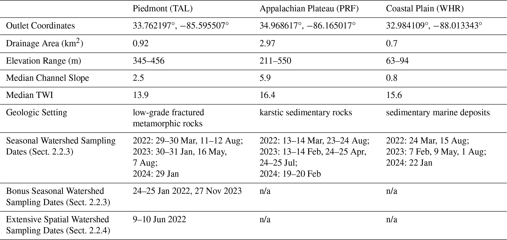
Table 1 Summary of watershed characteristics and dates for seasonal (Sect. 2.2.3), “bonus” seasonal, and extensive spatial (Sect. 2.2.4) watershed sampling campaigns. The bonus seasonal sampling campaigns are only in one watershed with data coverage limited to just hydrologic and water chemistry variables (e.g., no microbial or macroinvertebrate data).

n/a – not applicable.

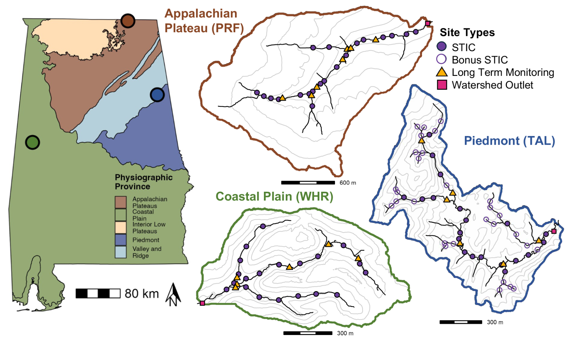
Figure 1 (left) Map of Alabama, USA with locations of the three study watersheds. Points shown on the Alabama map as well as the outlines of the Piedmont (Talladega; TAL; right, blue), Appalachian Plateau (Paint Rock; PRF; top, brown), and Coastal Plain (Shambley Creek; WHR; bottom, green) study watersheds are colored based on their respective physiographic province. Locations of water presence-absence sensors (STIC; purple circles), long-term monitoring sites (gold triangles), and watershed outlet monitoring sites (pink squares) in the stream network are shown on each watershed map (Sect. 2.2.1). Additional water presence-absence sensors (Bonus STIC; open circles with purple outline) were installed in the Piedmont study watershed during 2022 to correspond with sites sampled during a spatially-extensive synoptic sampling campaign in June 2022 (Sect. 2.2.4). Contours in each watershed map refer to relative elevation change throughout the watershed.

2.1.1 Piedmont (TAL)

Our focal study watershed in the Piedmont physiographic province is a 0.92 km² watershed within the larger Talladega National Forest (TAL; Table 1, Fig. 2). This watershed is entirely forested and located within federally owned public lands (953 km²) managed primarily for recreation, conservation, and silviculture. The watershed has moderate topographic relief with elevation ranging from 345 to 456 m above sea level (m a.s.l.) and forms an unnamed non-perennial tributary to Pendergrass Creek in Cleburne County (AL, USA), which is in the larger Coosa River and Mobile-Tombigbee River basins. Geologically, this watershed is underlain by low-grade metamorphic rocks, primarily interbedded phyllite, metasiltstone, and quartzite units that are heavily fractured due to their proximity to the Talladega fault (Szabo et al., 1988; Cook, 1982; Kopaska-Merkel et al., 2000). The watershed is dominated by highly weathered Ultisols, with thin, rocky slopes in the headwaters and with more organic, fine-grained soils near the outlet (Soil Survey Staff, 2025; Zarek et al., 2025). The dominant vegetation type in the region is oak-hickory-pine, and the watershed is a mixed deciduous-coniferous forest with primarily pine (loblolly, longleaf) and oak (mixed red and white) species (Griffith et al., 2001; Feminella, 1996). Additionally, this watershed experiences low-intensity prescribed burns for habitat management, including during our study in early spring 2022 and 2024.

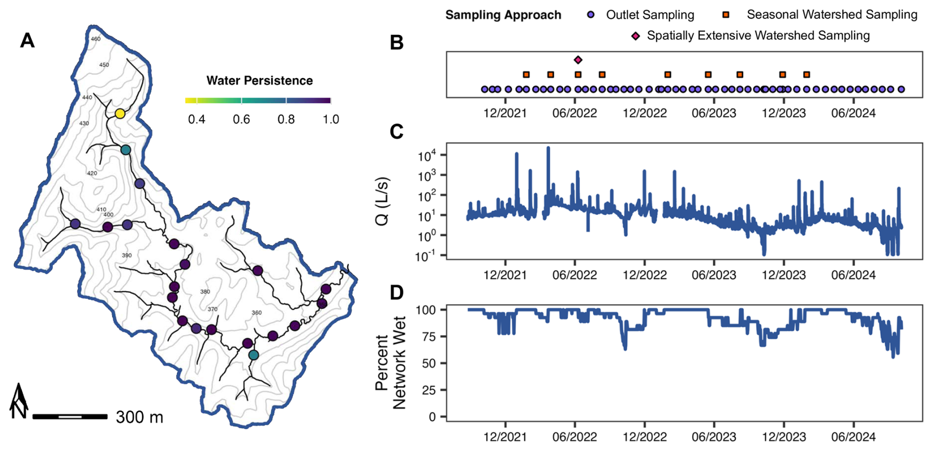
Figure 2 (A) Water persistence over the study period (September 2021–October 2024) at each water presence-absence sensor site across the Piedmont study watershed (TAL). Light colors indicate less continuous water persistence and darker colors indicate more continuous water persistence. (B) Sampling dates, (C) discharge at the watershed outlet (Q; L s⁻¹) and (D) percent network wet using the water presence-absence sensor network (Sect. 3.2.2) across the study period. For a given sampling date, purple circles refer to temporal sampling at the watershed outlet (Sect. 2.2.2) and orange squares for seasonal watershed sampling at the seven long-term monitoring sites (Sect. 2.2.3) and pink diamonds for an extensive spatial synoptic sampling campaign across the watershed (Sect. 2.2.4). Contours in the watershed map refer to relative elevation throughout the watershed.

2.1.2 Appalachian Plateau (PRF)

Our study watershed in the Appalachian Plateau physiographic province, Paint Rock (PRF), is a 2.97 km² watershed in Jackson Country, AL (USA; Table 1, Fig. 3). Almost entirely forested, the Appalachian Plateau watershed is privately owned and managed for hunting and conservation. This watershed drains Miller Mountain and Fanning Hollow to form an unnamed tributary to Burks Creek, which is in the larger Paint Rock River and Tennessee River basins. This is the highest relief watershed with elevation ranging from 211 to 550 m a.s.l. Geologically, this watershed is underlain by karst sedimentary rocks, primarily sandstones interbedded with shales, limestone, dolomite, and mudstones (Szabo et al., 1988), and the headwaters are located in the exposure of the limestone unit that yields the majority of caves and karst features in the state (Ponta, 2018). Due to the steep slopes and geologic erosion, the watershed mostly contains thin, stony soils within the Ultisol and Mollisol soil orders (Soil Survey Staff, 2025). Most soil formation and sediment accumulation occurs in the lower portion of the network, with exposed bedrock benches forming the stream channels in the headwaters (Soil Survey Staff, 2025). The forest structure is primarily deciduous, with dominant vegetation types of mixed oaks (chestnut, white, and red) in the upper slopes, mesic forest (beech, yellow poplar, sugar maple, basswood, ash, and buckeye) in the middle and lower slopes, and riparian zones with river birch and hemlock (Griffith et al., 2001).

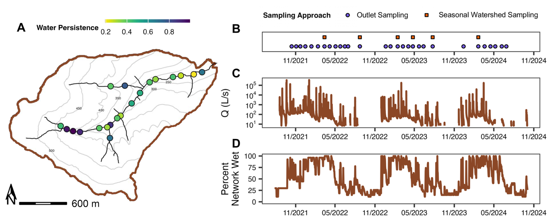
Figure 3 (A) Water persistence over the study period (August 2021–October 2024) at each water presence-absence sensor site across the Appalachian Plateau study watershed (PRF). Light colors indicate less continuous water persistence and darker colors indicate more continuous water persistence. (B) Sampling dates, (C) discharge at the watershed outlet (Q; L s⁻¹) and (D) percent network wet estimated using the water presence-absence sensor network (Sect. 3.2.2) across the study period. For a given sampling date, purple circles refer to temporal sampling at the watershed outlet (Sect. 2.2.2) and orange squares for seasonal watershed sampling at the seven long-term monitoring sites (Sect. 2.2.3). Contours in the watershed map refer to relative elevation throughout the watershed.

2.1.3 Coastal Plain (WHR)

Our study watershed in the Coastal Plain physiographic province, Shambley Creek (WHR), is a 0.70 km² watershed in Greene County, AL (USA; Table 1, Fig. 4). This watershed is entirely forested and is privately owned by the Weyerhaeuser Company and managed for rotational silvicultural harvest. This watershed drains the unnamed headwaters of Shambley Creek, which is in the larger Sipsey River and Mobile-Tombigbee River basins. This is the lowest relief watershed with elevation ranging from 63 to 94 m a.s.l. Geologically, this watershed is underlain by sedimentary units, primarily interbedded clay and sand layers that are one of the integral water-bearing units in the region (Szabo et al., 1988). This watershed is dominated by highly-weathered Ultisols, and the low relief paired with easily erodible soil textures has resulted in highly incised channels in the lower half of the watershed. This region has a historic forest structure of mixed coniferous and deciduous species (oaks, hickory, and pine; Griffith et al., 2001). However, in this watershed, the uplands are almost entirely pine with dense riparian species (i.e., gum, holly, sycamore). The southern portion of this watershed was thinned and harvested in summer 2024, but harvest only occurred in the uplands (i.e., all forest within ∼ 8 m of the channel was preserved).

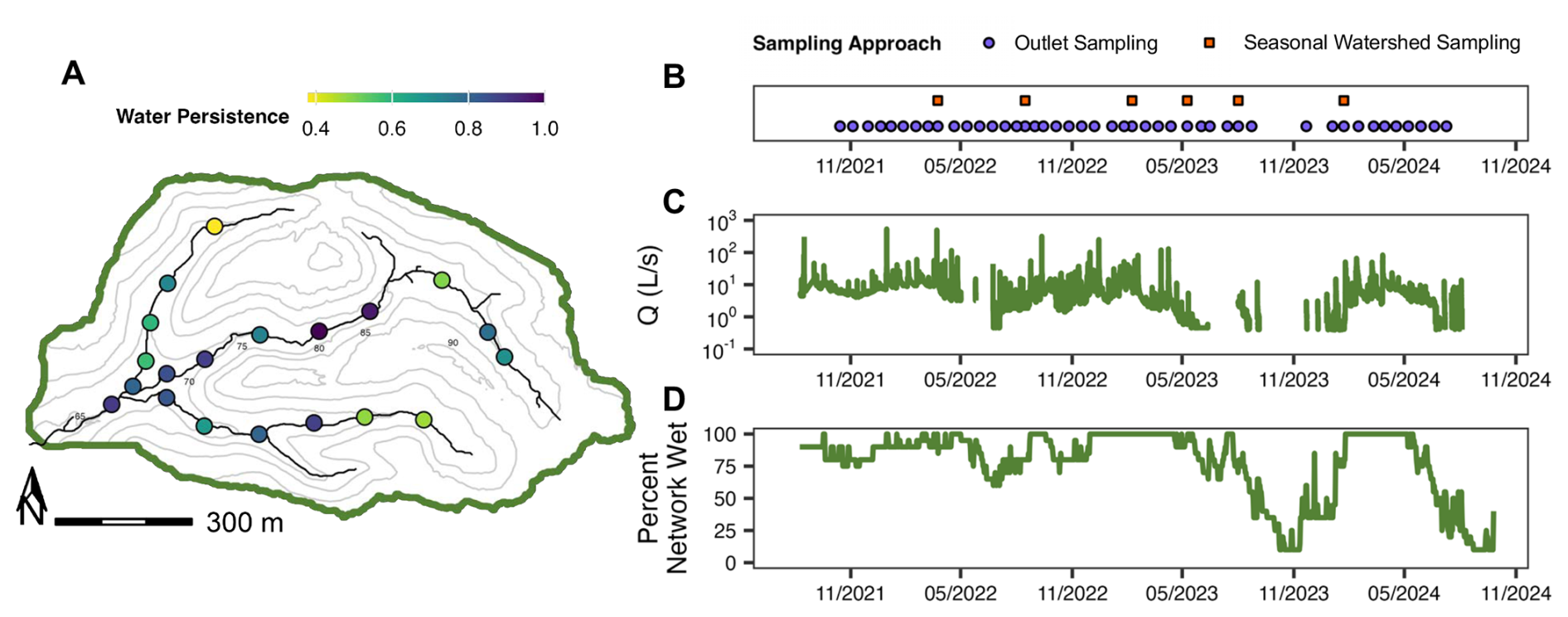
Figure 4 (A) Water persistence over the study period (August 2021–October 2024) at each water presence-absence sensor site across the Coastal Plain study watershed (WHR). Light colors indicate less continuous water persistence and darker colors indicate more continuous water persistence. (B) Sampling dates, (C) discharge at the watershed outlet (Q; L s⁻¹) and (D) percent network wet using the water presence-absence sensor network (Sect. 3.2.2) across the study period. For a given sampling date, purple circles refer to temporal sampling at the watershed outlet (Sect. 2.2.2) and orange squares for seasonal watershed sampling at the seven long-term monitoring sites (Sect. 2.2.3). Contours in the watershed map refer to relative elevation throughout the watershed.

2.2 Watershed study design

2.2.1 Sensor monitoring networks

Within each study watershed, we deployed high spatial-resolution sensor monitoring networks that maximized continuous data collection with multiple data types (Table 2). These monitoring networks were developed using a standardized site design that targeted both key locations within the network (i.e., tributary confluences, the watershed outlet) and randomly distributed sites across a gradient of topographic conditions (Swenson et al., 2024; Zipper et al., 2025a). Altogether, integrating across these different sensor types and network locations provides both the context of hydrologic connectivity and the downstream water-quality consequences for the rest of this project. The different components of these sensor networks can be divided into three categories: (1) multi-parameter water quality sondes located at the watershed outlet (n=1 site per watershed), (2) long-term monitoring sites consisting of in-stream stilling wells and piezometers instrumented with pressure transducers (n=7 sites, including the watershed outlet), (3) water presence-absence sensors throughout the watershed (STICs; n=20 sites). We also deployed and maintained local weather stations recording barometric pressure, rainfall, temperature, relative humidity, wind direction and speed, and photosynthetically active radiation. All weather stations were located in the nearest open-canopy location within 5 km of the watershed outlet, though both the Appalachian Plateau and Coastal Plain locations were within 1 km of their respective watershed outlet.

Table 2 Summary of watershed characteristics and time series data products collected in the Piedmont (TAL), Appalachian Plateau (PRF), and Coastal Plain (WHR) watersheds. Data products include: geospatial information for each sampling and monitoring site in each watershed (ENVI; Sect. 3.1), meteorological data collected from nearby weather stations (METS; Sect. 2.2.1), water presence-absence data from twenty sites in each watershed (STIC; Sect. 3.2.2); surface and ground water level data from seven sites in each watershed and including the watershed outlet (PRES; Sect. 3.2.1); discharge (DISC; Sect. 3.2.1), water quality from multi-parameter sondes (EXOS; Sect. 3.2.3), and absorbance spectra from submersible spectrophotometers (SCAN; Sect. 3.2.4) from the watershed outlets. All sensor-derived parameters were measured at 15 min intervals for the duration of the study (Autumn 2021–Autumn 2024). Further details on sensor monitoring network design, installation, and maintenance can be found in Sect. 2.2.1. Data products are published separately for each watershed and have been assigned unique data product citation identifiers, which can be used to find the full data product citation in Table A1.

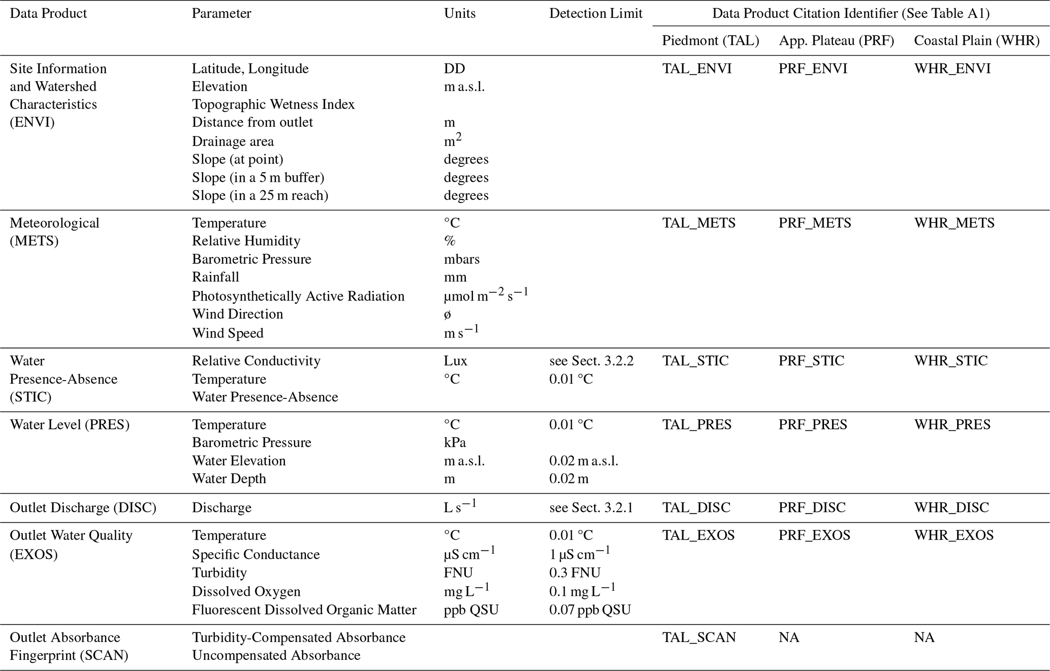
NA – not available.

The long-term water quality monitoring sites at each of the study watershed outlets consisted of an EXO2 multi-parameter water quality sonde (YSI, Ohio USA) measuring temperature (°C; instrument accuracy = ±0.01 °C), conductivity and specific conductance (µS cm⁻¹; instrument accuracy = ±1 µS cm⁻¹), turbidity (FNU; instrument accuracy = ±2 % up to 1000 FNU; ±5 % between 1000–4000 FNU), dissolved oxygen concentration (DO; mg L⁻¹; instrument accuracy = ±0.1 mg L⁻¹), and fluorescent dissolved organic matter concentration (fDOM; ppb QSU; instrument accuracy = ±0.01 ppb QSU), an installed stilling well and piezometer outfitted with vented pressure transducers to measure changes in surface water and groundwater level, and a pressure transducer deployed in the riparian zone to measure local changes in air temperature and barometric pressure (Fig. 1, Table 2). All sensors were set to collect measurements at 15 min intervals throughout the duration of the study. At the outlet of our focal, Piedmont study watershed, we also deployed a spectro::lyser V3 UV-Vis spectrophotometer (s::can, Badger Meter, Milwaukee, Wisconsin USA) to measure light absorbance at wavelengths from 190 to 750 nm at 2.5 nm intervals. Prior to collecting each reading, the EXO and UV-Vis spectrophotometer cleaned the lenses in their optical sensors using an automatic wiper. We conducted regular cleaning and maintenance of all sensors at the watershed outlets every three weeks and recalibrated the EXO water quality sondes every three months (Seybold, 2024).

The seven long-term monitoring sites distributed throughout the watersheds were selected to capture a gradient of drainage area accumulation (25 %, 50 %, and 75 %, located on the mainstem of the network), as well as the confluences of two primary tributaries in each network (Fig. 1). At each long-term monitoring site, co-located stilling wells and subsurface piezometers were installed in the thalweg and instrumented with Onset HOBO U20L pressure transducers (Onset Corporation, Massachusetts, USA) to measure stream water level and vertical head gradients at 15 min intervals. Stilling wells consisted of 2 in. (5 cm) diameter PVC installed initially such that the sensor port was within 2 cm of the streambed. In mid-2022, stilling wells were reinstalled such that the sensor port was approx. 10–20 cm below the streambed, but the well was screened above and below the streambed to capture surface water level. Further, piezometers were installed approximately 50 cm below the streambed, with a 20 cm screened interval to capture groundwater level. These locations were maintained every 4–6 months, when sensors were downloaded and relaunched, and physical measurements of water level were taken to ground-truth sensor observations (Zipper et al., 2025a).

The water presence/absence monitoring sites consisted of STIC sensors distributed throughout the watershed to capture a range of topographic conditions. Prior to deployment, STICs were calibrated to ensure accurate readings in the field (Burke et al., 2024). We utilized a standardized site design (see Zipper et al., 2025b for more information) to select locations randomly across a gradient of drainage area and topographic wetness index (hereafter, TWI; Swenson et al., 2024). At each location, a STIC sensor was placed at the highest point in the thalweg of the reach, such that it would capture the first point of network disconnection. The sensor was attached to a ∼ 1 m aluminum U-post using hose clamps and installed such that the sensor pins were within 1 cm of the stream bed. These sensors were used to measure continuous water presence or absence across the network for the duration of the project. STIC sensors were maintained every 4 months and had their batteries changed every 9 months (Godsey et al., 2024a). Additionally, at every maintenance visit, we collected observations of water presence or absence and recorded the height of sensor pins relative to the bed to account for any sediment accumulation or erosion. Further, in the Piedmont watershed, an additional 29 (“bonus”) STIC sensors were deployed for 11 months starting in May 2022 prior to the spatially extensive sampling campaign (see Sect. 2.2.4). We deployed bonus STIC sensors in locations where distances between permanent STIC sensors were large and along more ephemeral channels to increase the spatial resolution of water permanence observations within the existing network and to better capture the network expansion and contraction at maximum extent of the geomorphic channel network (Fig. 1).

2.2.2 Temporal sampling at the watershed outlet

Between Autumn 2021 and Autumn 2024, we visited the outlet of each watershed every three weeks to assess how flow, hydrologic connectivity, and water quality changed over the course of the study. During these tri-weekly site visits, we conducted regular sensor maintenance, measured hydrologic parameters, and collected water chemistry samples. Hydrologic parameters such as discharge and velocity were only collected if the reach upstream of the outlet sampling site was fully connected and flowing continuously for a distance of at least ten wetted widths. Water samples were only collected if water was present at the outlet (see Sect. 3.3.1). Our temporal outlet sampling data consists of 53, 29, and 44 timepoints for our Piedmont (TAL; Fig. 2B), Appalachian Plateau (PRF; Fig. 3B), and Coastal Plain (WHR, Fig. 4B) watersheds, respectively.

2.2.3 Spatiotemporal sampling across watersheds

To capture variability in watershed-scale hydrologic connectivity, water chemistry, and community dynamics, we conducted three synoptic sampling campaigns at the long-term monitoring sites within each study watershed per year for two years. These sets of seasonal synoptic campaigns across the three watersheds were aligned with expected seasonal dynamics in flow and connectivity, with a high baseflow campaign occurring in March–May, a dry-down campaign occurring in August, and a wetting-up campaign occurring in January–February. Sampling campaigns within the same seasonal watershed sampling set were conducted across all three watersheds within 2–3 weeks of each other, with sampling campaigns within a single watershed taking 1–2 d to complete. During each of these seasonal watershed sampling campaigns, we co-collected samples and data for hydrologic (Sect. 3.2), biogeochemical (Sect. 3.3), and microbial community (Sect. 3.4) parameters at the seven long-term monitoring sites located throughout each of the study watersheds (including the outlets). Hydrologic parameters such as discharge were only collected if the reach upstream of the sampling site was flowing, while water chemistry samples were only collected if water was present at the sampling site. Two additional seasonal watershed sampling campaigns were conducted in January 2022 and November 2023 in our focal Piedmont (TAL) watershed (1) to test our sampling design and methods and (2) to supplement other ongoing projects in the focal watershed. However, these additional seasonal synoptic campaigns only include limited hydrologic and biogeochemical data products. Lastly, DNA metabarcoding samples for macroinvertebrate community analyses were only collected during the first year of seasonal watershed sampling campaigns.

2.2.4 Extensive spatial synoptic sampling across Piedmont (TAL) watershed

We conducted a spatially extensive synoptic sampling campaign from 9–10 June 2022 in the focal Piedmont watershed to capture network-scale patterns and drivers of water persistence, chemistry, and resultant biotic communities. During this sampling campaign, we co-collected samples for biogeochemical parameters (Sect. 3.3) and microbial community analyses (Sect. 3.4) at all permanent STIC, bonus STIC, and long-term monitoring sites (including the watershed outlet; n=50 sites). We only collected samples for biogeochemical parameters and water column microbial community analyses at sites with surface water present at the time of sampling (n=38 sites). Additionally, we co-collected samples and data for macroinvertebrate community and hydrologic parameters at a subset of sites (n=20 sites for hydrologic parameters and n=28 sites for macroinvertebrate community analyses) as the stream reach lengths required for our field methods for these parameters were longer than actual reach lengths between many of our sites in this campaign (see Sect. 3.1.2 for hydrologic parameters and Sect. 3.5 for macroinvertebrate community analyses). We selected this subset of sites to maximize spatial resolution and connectivity variation of our hydrologic and macroinvertebrate community data across the network. To minimize interference and potential contamination, we coordinated our efforts by splitting sampling teams by discipline and sequentially sampled microbial community analyses, biogeochemical parameters, macroinvertebrate community, and hydrologic parameters analyses from downstream to upstream.

3 Methods

3.1 Site characterization (ENVI)

All sensor locations (latitude, longitude) were measured with an eMLID Reach RX multi-band RTK rover with sub-meter accuracy (eMLID Tech Kft., Hungary). Using these high-resolution sensor locations, we calculated a suite of topographic metrics to contextualize our results: drainage area, distance from outlet, slope, channel slope, slope buffer, and stream slope (Peterson and Jones, 2026a, b, c). First, we obtained 1 m resolution (or finer) DEMs from USGS TNMD v2.0 (https://apps.nationalmap.gov/downloader/, last access: 7 May 2025) and performed all analyses in R v4.4.0. DEMs were processed (filtered, pits filled, depressions breached) using the whitebox R package before being cropped to our delineated watershed extent (Wu and Brown, 2022). Stream networks were delineated in whitebox using thresholds that most closely matched field observations of the geomorphic channel network extent (Piedmont = 10 000 0.92 m cells; Coastal Plain = 12 000 1 m cells; Appalachian Plateau = 60 000 1 m cells). We calculated drainage area, distance from outlet, slope, continuous channel slope, and TWI rasters using their respective whitebox functions. Drainage area, distance from outlet, slope point, and TWI were extracted from their respective rasters using the high-resolution site locations. Slope buffer was calculated by averaging all raster cells within a 5 m buffer of the locations to integrate local slope. Stream slope was calculated by averaging all continuous channel slope raster cells within the 25 m reach surrounding the location.

3.1.1 Site-level discharge estimates (DISL)

Between August 2021 and October 2024, we conducted solute-pulse tracer additions of sodium chloride to measure discharge and velocity along the stream reach immediately upstream at each sample site as described in McCleskey et al. (2025) and Godsey et al. (2024b; Table 3). Tracer additions were only conducted if the reach upstream of the sample site was fully connected and flowing continuously for a distance of at least ten wetted widths. During these tracer additions, a known mass of sodium chloride dissolved in stream water was added instantaneously to the stream while specific conductance (in µS cm⁻¹) was monitored continuously using two conductivity loggers (Solinst) measuring conductivity every 2 s at a downstream monitoring site approximately 10–20 wetted widths from the tracer addition site to ensure complete mixing of the tracer across the stream channel prior to its arrival. We conducted these tracer additions to measure discharge at the watershed outlets every three weeks during maintenance visits, seasonally at the seven long-term monitoring sites, and at n=20 sites in the focal watershed during the extensive spatial synoptic campaign in June 2022 (Table 1, Figs. 2A, 3A, 4A).

Table 3 Summary of field measurements and sample-based water chemistry and dissolved gas data products collected in the Piedmont (TAL), Appalachian Plateau (PRF), and Coastal Plain (WHR) watersheds. Data products include field measurements of physicochemical parameters (YSIS), site-level streamflow estimates (DISL; Sect. 3.1.2), seston concentrations (TSSS; Sect. 3.3.1), dissolved nutrient, anion, cation, and dissolved organic carbon concentrations (NUTR, ANIO, CAIO, DOCS; Sect. 3.3.2), dissolved organic matter optical properties (DOMS; Sect. 3.3.3), water isotopes (WAIS; Sect. 3.3.4), and dissolved gas concentrations (MIMS, GHGS; Sect. 3.4.1). In all three watersheds, samples for YSIS, DISL, NUTR, ANIO, CAIO, DOCS, DOMS, and WAIS were collected at all sites on all sampling dates for each sampling approach (Sect. 2.2.1–2.2.3) for the full study period (Autumn 2021–Autumn 2024). Sampling for dissolved gasses were limited to seasonal watershed sampling events (all three watersheds for MIMS, Piedmont only for GHGS) and the spatially-extensive Piedmont synoptic campaign. Further details on sample collection and analysis for water chemistry and dissolved gasses can be found in Sect. 3.3–3.4. Data products are published separately for each watershed and have been assigned unique data product citation identifiers, which can be used to find the full data product citation in Table A1.

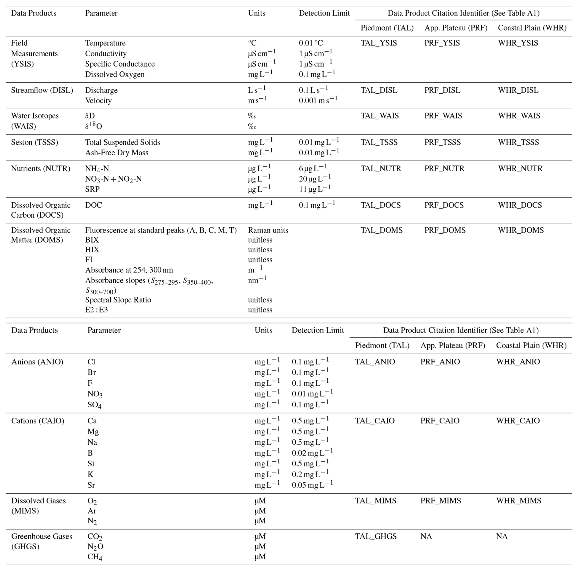
NA – not available.

3.2 Sensor data processing and quality assurance

3.2.1 Water level and rating curves for continuous discharge (PRES, DISC)

We converted raw sensor data to absolute water level for every stilling well and piezometer. Briefly, raw pressure data from unvented, HOBO U20L sensors (i.e., all long-term monitoring sites, and the outlet monitoring stations beginning in 2023; maximum sensor error = 0.43 kPa) were converted to water pressure using an elevation-corrected, barometric pressure transducer deployed within the study watershed (Tables 2, A1). This sensor water pressure was converted to water level relative to the sensor-specific datum by correcting for the specific weight of water. Additionally, the outlet monitoring stations were originally instrumented with Seametrics PT12 pressure sensors that recorded relative stream water level (the Piedmont sensor was replaced in January 2023, the Coastal Plain was replaced in June 2023, and the Appalachian Plateau was replaced in June 2024). For all sensors, this relative water level was then converted to absolute water level (waterElevation, in meters above sea level) using field-observed water level and surveyed elevation data. Further, we calculated water level relative to the average streambed elevation using field observations (waterDepth, m). We manually measured water level and streambed elevation during every sensor maintenance (i.e., every 4–6 months) and used these observations to correct sensor measurements. The potential error introduced by removing sensors for downloading data is greater than the potential drift of sensor measurements; therefore, these manual adjustments compensated for this source of uncertainty. Moreover, any level measurements recorded within the lower range of sensor uncertainty (i.,e., <2 cm of relative water level) were removed and flagged with a “dry” value in the “wetdry” column and a D flag in the “QAQC” column.

Using discharge estimates measured at the outlet of each watershed, we developed site-specific discharge-stage rating curves to estimate discharge at 15 min intervals (Gore and Banning, 2017). This approach allowed us to capture a distribution of flow conditions in each watershed over the three-year study (Figs. 2C, 3C, 4C). However, our assessment of the stage-discharge relationship during high-flow events is limited by the lack of stormflow discharge estimates. We therefore constrained the upper limit of our stage-discharge rating curves to stage measurements less than bank-full stage estimated from on-site topographic surveying. Any discharge measurements recorded within the lower range of sensor uncertainty (<2 cm of relative water level), that were greater than 200 % of our highest measured discharge estimates at a given site, and that were less than half of the highest measured discharge estimates at a given site, were flagged as “D”, “M”, or “L” in the “QAQC” column, respectively.

3.2.2 Water presence-absence (STIC)

We deployed at least 20 STIC sensors in each of our three watersheds to measure water presence or absence continuously throughout the network. These sensors, modified sensu Chapin et al. (2014) from a HOBO Pendant logger, recorded temperature and relative conductivity (in lux) at 15 min intervals. Then, using a project-wide reproducible workflow outlined in Zipper et al. (2025b), we converted relative conductivity to binary water presence or absence based on sensor-specific thresholds identified through laboratory calibrations (Figs. 2A, 3A, 4A). To account for sensor drift, laboratory calibrations were performed annually, and we adjusted the thresholds for water presence or absence as needed. These water presence/absence observations were then compared to field observations, quality-checked, and flagged based on data quality. While a universal measure of uncertainty could not be provided due to the modification of the sensors, confidence in the binary water presence/absence measurements is denoted in the “qual_rating” column, where data gaps, sediment accumulation or erosion, and agreement with field observations were used to provide a qualitative measure of confidence in data quality. Moreover, potentially anomalous presence/absence measurements (i.e., a short period of “dry” surrounded by a long period of “wet” as calculated by a moving window z-score of relative conductivity) were flagged with a D in the “QAQC” column.

To capture expansion and contraction dynamics in each stream network, we used data from all permanent STIC sensors within each watershed to estimate the percent of active network wet at each timepoint as the number of wet STIC sensors normalized for the total number of STIC sensors (Figs. 2D, 3D, 4D). Prior to calculating percent network wet for each watershed, we removed STIC sensors where >50 % of measurements received a poor data quality flag over the study period (n=0 sensors for TAL, n=1 for PRF, n=6 for WHR), estimated daily wet/dry conditions at each site as the daily mode of each 15 min STIC time series, and interpolated data gaps for up to two days using the STIC.RFimpute() function in the StreamDAG R package (Aho et al., 2023).

3.2.3 Multi-parameter water quality sondes (EXOS)

Prior to any parameter-specific corrections or analyses, we used a standardized protocol to check and assure the quality of our high-frequency water quality data collected using the EXO2 multiparameter sondes deployed at each of our watershed outlets (Fig. 5). We first identified and filtered out unrealistic values in each of the temperature, conductivity, specific conductance, dissolved oxygen concentration, and turbidity time series using (1) an alpha filter to remove erroneous values (e.g., error code readings, negative concentrations) and (2) a conservative beta filter that removed measurements that were greater than three standard deviations of a rolling mean or greater than three moving absolute deviations. We then manually checked and flagged any remaining time periods of instrument malfunction, burial, and desiccation using field notes, water level data collected from the co-located stilling well, and sudden baseline shifts in the conductivity and turbidity data from the watershed outlet (Fig. 5).

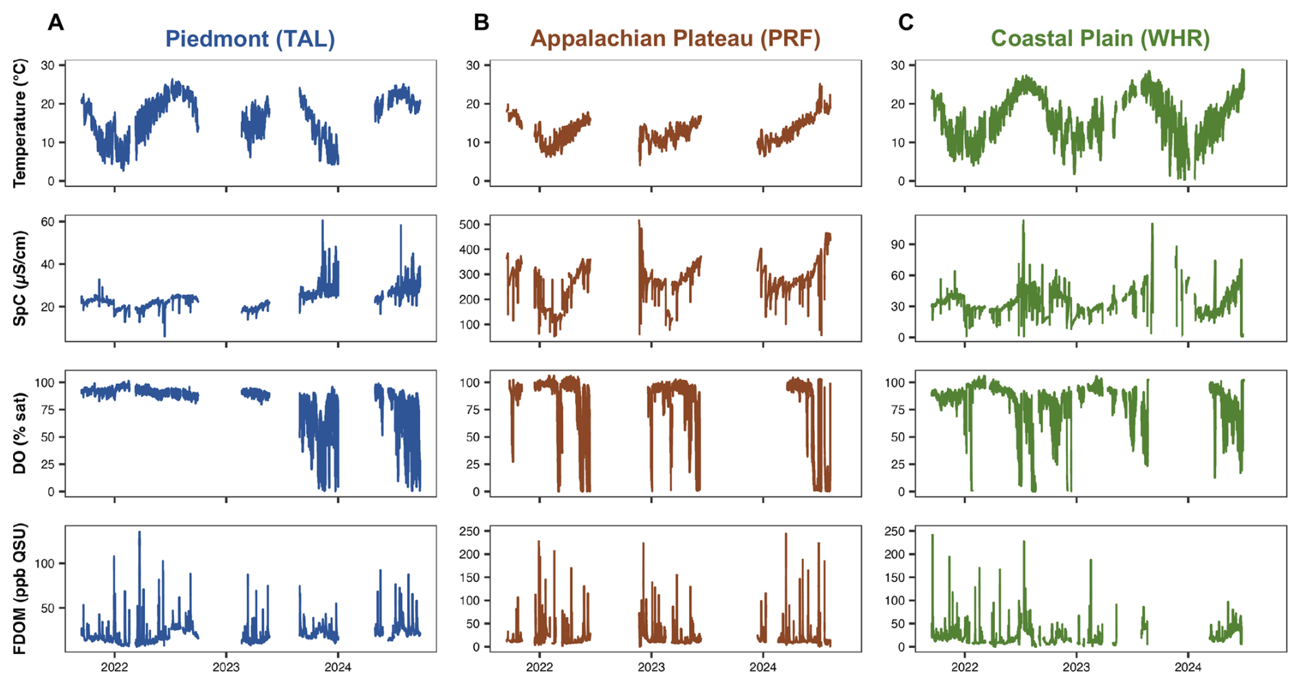
Figure 5 Time series of temperature (°C; first row), specific conductance (SpC; µS cm⁻¹; second row), dissolved oxygen (DO; % saturation; third row), and fluorescent dissolved organic matter (FDOM; ppb QSU; fourth row) at the watershed outlet over the deployment period in the Piedmont (TAL; A), Appalachian Plateau (PRF; B), and Coastal Plain (WHR; C) study watersheds. FDOM concentrations are compensated for temperature and turbidity effects following methods outlined in Sect. 3.2.3. Data gaps in time series are due to either dry conditions, burial, sensor malfunction, or sensor maintenance, each of which are flagged in the published data sets.

To determine the potential for signal drift in water quality sensors, we compared pre- and post-calibration values of calibration standards and checks (e.g., distilled water allowed to equilibrate to room temperature and local conditions) for temperature, specific conductance, dissolved oxygen, turbidity, and fluorescent dissolved organic matter during routine sensor calibration conducted every three months. When signal drift for a given parameter exceeded 10 % (as the difference in pre- and post-calibration values), we then implemented a parameter-specific, linear baseline shift to correct data since the previous calibration. Overall, the high degree of expected, temporal variability in water quality parameters due highly variable stream flow and connectivity over the course of the study period prevented us from a more conservative assessment of potential sensor drift influences. However, we expect the influence of water quality sensor drift to be minimal due to the frequency of our sensor maintenance and recalibration over the study period.

We corrected fDOM measurements for both instrument- and site-specific effects of temperature as well as suspended and dissolved particles that can influence the attenuation of light in water (Fig. 5). Briefly, we used methods described in Watras et al. (2011) and the EXO User Manual (Yellow Springs Instruments, 2020) to compensate raw fDOM measurements for temperature effects on fluorescent intensity using a reference temperature of 25 °C and a specific temperature attenuation coefficient of −0.01 °C⁻¹. We tested for potential filtering effects due to dissolved particles in the water, or the inner filter effect, and suspended particles following laboratory methods described in Downing et al. (2012). We determined that inner filter effects likely played a negligible role in influencing fluorescence intensity measurements at our sites given consistently low absorbance values in site-specific filtered water, even when turbidity exceeded 1000 FNU, and decided not to include inner filter-effect fDOM corrections. We corrected for the influence of suspended particles, assessed as turbidity, on fDOM measurements following methods adopted from Downing et al. (2012) and Senatore et al. (2023). We estimated the turbidity attenuation factor for each fDOM sensor by first calculating the ratio of temperature-compensated fDOM measurements and measured dissolved organic carbon (DOC) concentrations from grab samples (fDOM/DOC) and fitting an exponential decay function to each fDOM/DOC vs. turbidity relationship, following expected trends of the Beer-Lambert Law. To derive these turbidity attenuation factors, we used paired fDOM, DOC, and turbidity measurements from samples collected in the field throughout the sensor deployment, as well as DOC samples and fDOM readings collected during laboratory tests in which we systematically increased turbidity to the highest recorded turbidity values from each site (∼ 1000 FNU) to simulate the highest flow-induced turbidity conditions in our deployment (Fig. 5). These turbidity attenuation factors were comparable to those reported by others in previous work using similar laboratory-correction procedures (Downing et al., 2012; Senatore et al., 2023).

3.2.4 UV-Vis absorbance fingerprint (SCAN)

Due to the complexity of the absorbance spectra time series generated by the submersible UV-Vis spectrophotometer (s::can spectro::lyser V3), we used a simplified version of our data quality-assurance methods for sensor-derived water chemistry to filter out erroneous absorbance spectra. We used error codes recorded on the instrument, field notes, and water-level and turbidity data from the watershed outlet to help remove all spectra during periods of instrument malfunction, burial, and desiccation. We further filtered the absorbance data time series by first selecting three wavelengths (200, 255, 400 nm) to be representative of the entire UV-Vis absorbance spectra. We removed entire recorded spectra when (1) absorbance values at a given time point were negative at 200 or 255 nm and (2) when absorbance values at a given time point exceeded three standard deviations of the rolling mean absorbance values at 200, 255, or 400 nm. We processed and opted to publish both the turbidity-compensated and uncompensated absorbance spectra time series for the entire deployment record (Table 2).

3.3 Water chemistry sampling and analysis

3.3.1 Sample collection

We collected surface water samples following standard operating procedures outlined by the “Aquatic Intermittency effects on Microbiomes in Streams” project (Burgin, 2024). During each sampling event, we collected water samples for dissolved organic carbon (DOC), nutrients including ammonium (NH₄-N), nitrate/nitrite (NO₃-N + NO₂-N), and soluble reactive phosphorus (SRP), anion, and cation concentrations, as well as water isotopes (δD, δ¹⁸O), dissolved organic matter optical properties, total suspended solids, and seston ash-free dry mass (AFDM) at a given site (Tables 3, A1). We filtered DOC samples through pre-ashed 0.7 µm glass fiber filters (Whatman GF/F) into triple-rinsed 60 mL amber high-density polyethylene (HDPE) bottles, acidified DOC samples to a pH of 2 using concentrated HCl, and refrigerated samples at 4 °C for up to 28 d prior to analysis. We filtered samples for nutrient, anion, and cation concentrations through sterile, 0.45 µm PVDF filter cartridges (VWR) into triple-rinsed 50 mL sterile centrifuge tubes for nutrients and 30 mL clear HDPE bottles for anions and cations, respectively. We kept nutrient and anion samples frozen and acidified cation samples to a pH of 2 using concentrated HNO₃, which were kept refrigerated at 4 °C until analysis. We collected samples for water isotopes by triple-rinsing and filling clear borosilicate sample bottles with conical caps underwater until no headspace remained in the sample to reduce potential evaporative fractionation. We then sealed caps of each water isotope sample with parafilm and stored at room temperature until analysis. For dissolved organic matter samples, we filtered water through 0.22 µm cellulose acetate filters into triple-rinsed 30 mL amber HDPE bottles until no headspace remained and then refrigerated until analysis. We collected triplicate samples for all surface water chemistry except for water isotopes, which we collected in duplicate. To measure total suspended solids and AFDM concentrations, we collected 2–3 replicates of unfiltered stream water in clean 1 L Nalgene bottles after triple-rinsing in the field, which were then stored on ice and brought to the lab for filtering. We vacuum-filtered known volumes of stream water within 24 h onto pre-ashed and pre-weighed 0.7 µm glass fiber filters (Whatman GF/F), placed in a drying oven at 50 °C for at least 48 h, and then weighed for the sample dry mass. We calculated total suspended solids concentration (in mg L⁻¹) as the sample dry mass normalized for the volume of water filtered. To determine AFDM concentrations, we ashed the dried sample filters at 500 °C for four hours, re-wet with Type 1 water, dried at 50 °C for at least 48 h, and weighed the remaining sample mass. We calculated seston AFDM concentration (in mg L⁻¹) as the difference in dry mass before and after ashing normalized for the volume of water filtered.

3.3.2 Dissolved water chemistry analysis (NUTR, ANIO, CAIO, DOCS)

After field sampling, samples were allowed to come to room temperature prior to analyses. We briefly describe water chemistry analysis below. Further details of instrument specifics and parameters for all analyses can be found in the metadata descriptions provided with each specific data publication in the AIMS Hydroshare repository (Tables 3, A1). We analyzed stream water samples for nutrient concentrations using an AQ300 Discrete Analyzer (SEAL Analytical, Mequon, Wisconsin, USA). Briefly, we determined dissolved organic carbon (DOC) concentrations as non-purgeable organic carbon (in mg L⁻¹; DOC method detection limit = 0.25 mg L⁻¹) via acid-catalyzed, high-temperature combustion using a Shimadzu TOC-V total organic carbon analyzer (Shimadzu Scientific Instruments, Kyoto, Japan). We analyzed samples for soluble reactive phosphorus (SRP; µg L⁻¹), ammonium (NH₄-N; µg L⁻¹), and nitrate/nitrite (NO₃-N + NO₂-N: µg L⁻¹) using the ascorbic acid method (SRP method detection limit = 6 µg L⁻¹; Murphy and Riley, 1962), phenol-hypochlorite method (NH₄-N method detection limit = 11 µg L⁻¹; Solórzano, 1969), and cadmium reduction method (NO₃-N method detection limit = 20 µg L⁻¹; APHA, 2017), respectively. While all water samples collected for nutrient determination were analyzed for SRP and NH₄-N, only samples collected before July 2024 were analyzed for NO₃-N using the cadmium reduction method. We determined aqueous concentrations of anions (fluoride [F], chloride [Cl], bromide [Br], nitrate [NO₃], and sulfate [SO₄]) using ion chromatography with either an IC-3000 IC system (Dionex, Sunnyvale, CA) with a Dionex IonPac AS15 column (2 mm by 50 mm, Thermo Scientific) for samples collected prior to January 2023 or a Metrohm 930 Compact IC Flex (Metrohm, Riverview, Florida) for samples collected after January 2023. We confirmed that anion concentrations were comparable between these two instruments within the range of standard error estimates typical of each analyte by running sets of paired water samples on each instrument (one-way analysis of variance, p = 0.851, df = 35). We also found that nitrate concentrations (in µg NO₃-N L⁻¹) were comparable between samples analyzed via cadmium reduction and via ion chromatography instrument (one-way analysis of variance, p = 0.782, df = 86). We determined aqueous concentrations of base cations (sodium [Na], calcium [Ca], boron [B], magnesium [Mg], silicon [Si], potassium [K], and strontium [Sr]) via inductively coupled plasma-atomic emission spectrometry (ICP-AES) using a Horiba Ultima 2 fitted with an AS 500 autosampler (Horiba Jobin Yvon). We re-filtered samples for base cation determination using a 0.2 µm PES filter immediately prior to analysis. All final sample concentrations or values that fell below method detection limits were flagged in the final datasets. Information pertaining to data quality flags for a given dataset type is included on the cover sheet of data files.

3.3.3 Dissolved organic matter characterization (DOMS)

Excitation-emissions matrices and absorbance spectra were collected for dissolved organic matter characterization on a Horiba Aqualog from 249 to 830 nm at 5 nm increments at the University of Alabama and/or Idaho State University. Integration times varied from 2 to 4 s, based on sample concentration. EEMs were blank-corrected, Raleigh masked, inner filter effects were removed, and values were Raman-normalized using Aqualog software. Standard fluorescence metrics were calculated from corrected EEMs using the StaRdom package (Pucher et al., 2019) in R (Tables 3, A1). These included: biological index (BIX; an indicator of autotrophic dissolved organic matter; Fellman et al., 2010), fluorescence index (FI; an indicator of relative terrestrial or microbial source of organic matter; McKnight et al., 2001), and humification index (HIX, an indicator of the extent of humification; Ohno, 2002). We also calculated fluorescence at standard peaks: amino acid-like peak tyrosine (B) and amino acid-like peak tryptophan (T), which both indicate labile protein-like dissolved organic matter; humic-like peaks A and C, which both indicate dissolved organic matter derived from terrestrial vascular plants, aromatic, likely higher-molecular weight dissolved organic matter; and humic-like peak M (M), which is considered less aromatic and lower molecular weight than peaks A and C (Coble, 1996; Fellman et al., 2010).

Absorbance metrics were also calculated in StaRdom (Tables 3, A1), including absorbance at 254 nm (a254; which is correlated with aromaticity; Weishaar et al., 2003), absorbance at 300 nm (a300; a proxy for photosensitive, chromophoric dissolved organic matter; Clark et al., 2019) and E2 : E3 (the ratio of absorbance at 250 nm to absorbance at 365 nm), which is negatively correlated with molecular weight and aromaticity (Li and Hur, 2017). We calculated absorbance slopes from 275–295 nm (S275_5295), 350–400 nm (S350_400), and 300–700 nm (S300_700), which are all proxies for molecular weight (Helms et al. 2008), slope ratio (SR; the ratio of the best-fit slopes of absorbance from 275–295 nm to the slope of absorbance from 250–400 nm) which is negatively correlated with molecular weight and sensitive to photobleaching (Helms et al., 2008).

3.3.4 Water isotope analysis (WAIS)

All water isotope samples were stored in darkness at room temperature until analysis. The first sample from each duplicate pair was designated for analysis, while the second served as an archive. Oxygen and hydrogen isotope ratios (δ¹⁸O and δD) were measured using a cavity ring-down spectroscopic isotope water analyzer (Picarro L2130-i, Picarro Inc., CA). For each sample, six sequential sub-samples were analyzed to account for memory effects. The first three sub-samples equilibrated the measurement cavity, while the final three sub-samples were used to calculate δ¹⁸O and δD ratios. To correct for instrument drift and ensure measurement precision, all samples were calibrated against internal secondary standards. The internal secondary standards were previously calibrated against International Atomic Energy Agency (IAEA) primary standards referenced to Vienna Standard Mean Ocean Water. All isotope values are reported as per mil (‰) deviations relative to VSMOW. Due to instrument malfunction, water isotope data is only available for samples collected before March 2023.

3.4 Dissolved gas sampling and analysis

3.4.1 Sample collection

Dissolved gas sampling of dinitrogen (N₂), oxygen (O₂), argon (Ar), carbon dioxide (CO₂), methane (CH₄), and nitrous oxide (N₂O) took place during all seasonal watershed sampling campaigns and the spatially-extensive Piedmont watershed synoptic campaign (Zarek and Burgin, 2025; Burgin et al., 2025). For seasonal watershed sampling campaigns, we collected samples for N₂, O₂, and Ar at the seven long-term monitoring sites in all three watersheds while samples for CO₂, CH₄, and N₂O were only collected in the Piedmont watershed. For the spatially-extensive Piedmont watershed synoptic campaign, samples for N₂, O₂, and Ar as well as for CO₂, CH₄, and N₂O were collected at 40 locations throughout the Piedmont watershed. For N₂, O₂, and Ar sampling, we used one 140 mL syringe with a two-way stopcock and long tubing extender attached on the end of the stopcock to collect a bubble-free water sample from the stream. Upon sample collection, we expelled 40 mL of water through the long tubing extender into three 12 mL vials (Exetainer^®, Labco, UK). In each vial, we overflowed the sample vial volume ∼ 3× before forming a meniscus and then preserving with 0.2 mL of 50 % ZnCl₂. Samples were capped, inverted to make sure there were no bubbles, and stored underwater in a container and on ice until we returned to the lab (Zarek and Burgin, 2025). Samples for CO₂, CH₄, and N₂O were collected using a headspace equilibrium technique (Burgin et al., 2025). Using a 60 mL syringe, we pulled 20 mL of a bubble-free surface water sample from the stream, and we pulled a 10 mL argon headspace into a 30 mL syringe. Then under water, we transferred the known volume of argon to the known volume of surface water and shook the syringe vigorously for 5 min to equilibrate the dissolved gases in the water with argon. After 5 min, 10–12 mL of headspace from each syringe was transferred to a 6 mL pre-evacuated vial (Exetainer^®, Labco, UK). All samples for CO₂, CH₄, and N₂O were collected in triplicate and stored in a container until we returned to the laboratory.

3.4.2 Dissolved gas analysis (MIMS, GHGS)

Samples for CO₂, CH₄, and N₂O were analyzed via a gas chromatograph equipped with a flame ionization detector and electron capture detector (Agilent7890B, Santa Clara, CA). We calculated CO₂, CH₄, and N₂O concentrations using Henry's Law and the Ideal Gas Law constants (Weiss, 1974; Weiss and Price, 1980; Wiesenburg and Guinasso, 1979; Tables 3, A1). N₂, O₂, and Ar were measured via a membrane inlet mass spectrometer. The concentrations of N₂, Ar, and O₂ were determined using the mimsy R package which calculates gas concentrations based on known solubility conditions, including barometric pressure, specific temperature, and salinity (Kelly, 2020; Tables 3, A1).

3.5 Microbial community collection and analysis

3.5.1 Field site characterization and sample collection

Sampling of microbial DNA, extracellular enzyme activity, chlorophyll-a (Chl-a), and habitat-specific ash-free dry mass (AFDM) took place during the seasonal watershed sampling campaigns in all three study watersheds (Sect. 2.2.3) and extensive spatial synoptic sampling campaign in the Piedmont study watershed (TAL) during June 2022 (Sect. 2.2.4) according to the AIMS microbial field sampling protocol (Zeglin and Busch, 2024; Table 1). Briefly, for each sampling event at each site, samples for microbial analyses were collected for each of four microbial habitat compartments: decaying leaf litter, rock surfaces (epilithon), benthic sediments, and surface water (Table 4). For each event at each site, samples collected from each habitat were subsampled for DNA, extracellular enzyme activity, and AFDM. Subsamples for Chl-a were collected for surface water and rock surfaces. In the field, DNA subsamples were flash-frozen and stored in liquid nitrogen and then transferred to a −80 °C freezer for storage in the lab, while extracellular enzyme activity, AFDM, and Chl-a samples were placed on dry ice in the field and −20 °C for storage in the lab. Further details on sample collection and site characterization are as follows.

Table 4 Summary of microbial and macroinvertebrate community data products collected in the Piedmont (TAL), Appalachian Plateau (PRF), and Coastal Plain (WHR) watersheds. Data products include field metadata for microbial (MIME; Sect. 3.5.1) and macroinvertebrate (MAME; Sect. 3.6.1) community sampling, habitat-specific measurements of ash-free dry mass (AFDM; Sect. 3.5.2) and chlorophyll a (CHLA; Sect. 3.5.2), DNA metabarcoding data for macroinvertebrate communities (MACR; Sect. 3.6.2), 16S and ITS sequencing data for microbial communities (Sect. 3.5.3), and habitat-specific extracellular enzyme activities (EEAS; Sect. 3.5.2). In all three watersheds, data for MIME, AFDM, CHLA, EEAS, and 16S/ITS sequencing of microbial communities were collected at all long-term monitoring sites on all sampling dates for each seasonal watershed sampling (Sect. 2.2.2) and for all sites during the spatially extensive watershed sampling campaign in the Piedmont watershed (Sect. 2.2.3). Macroinvertebrate community sampling (MAME, MACR) was limited to just the Piedmont (TAL) and Coastal Plain (WHR) watersheds for all three sampling approaches on dates between November 2021 and January 2023. Data products are published separately for each watershed and have been assigned unique data product citation identifiers, which can be used to find the full data product citation in Tables A1 and A3.

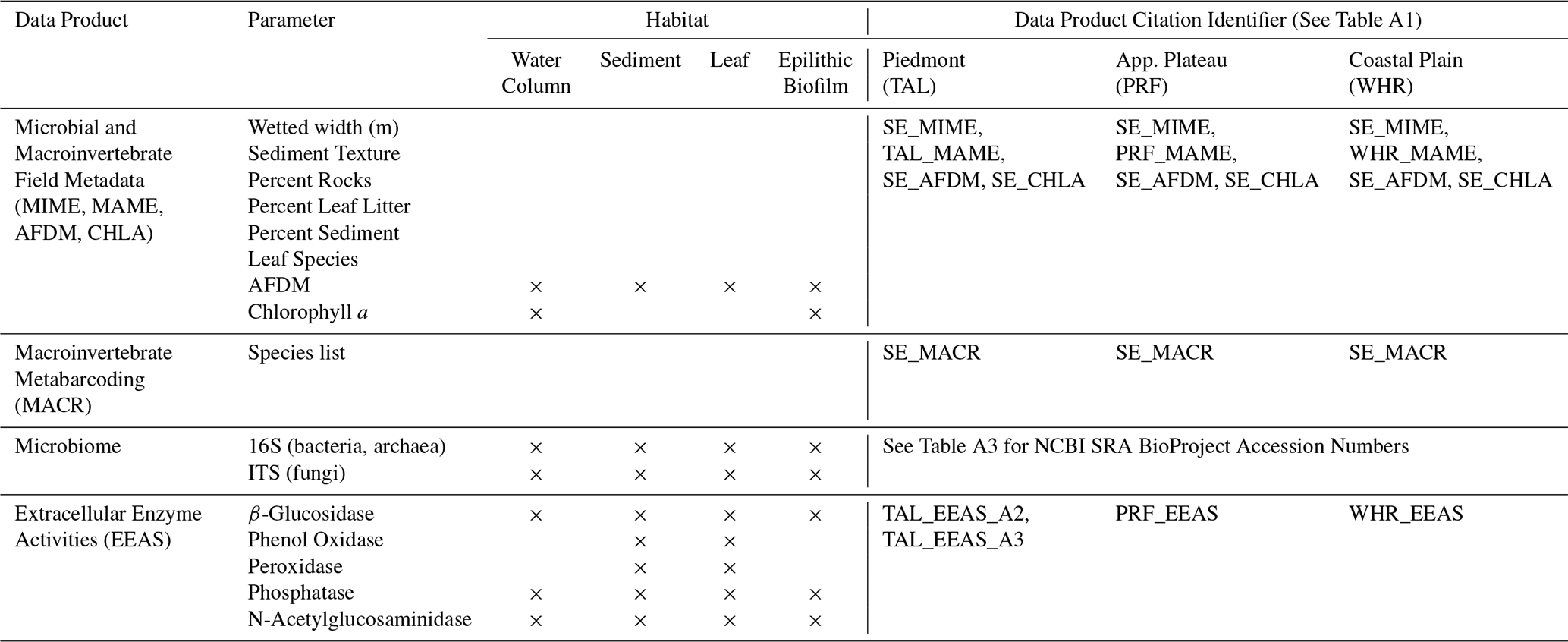
At each site, we defined the sampling area as the full wetted width of the stream centered on the in-stream sensors for that site. For the outlet sites in each watershed, where the sensors were in pools too deep to sample, sampling took place in a shallower transect immediately adjacent to the sensor pool. At dry sites, sampling areas were determined based on visual indicators of past water level. Each sampling area was divided into three subsampling areas (sub-areas) of equal width. All four microbial habitat compartments were sampled in each sub-area. The same amount of habitat-specific material was collected for each sub-area of a site, which was then combined to make a habitat-specific composite sample for each site.

Water was collected first to prevent benthic disturbance from contaminating the sample. Using a sterile 60 mL syringe, 120 mL of surface water was collected from each of the three subsampling areas and combined in a 500 mL Nalgene bottle. Water samples were subsampled for DNA by filtering up to 120 mL (or until the filter clogged) onto a sterile 0.22 µm cellulose acetate filter, and up to 60 mL each were filtered onto GF/F filters for Chl-a and water column AFDM. For epilithic biofilms, one rock was collected from each subsampling area, scraped using a sterile wire brush over a 25 cm² surface area on the top of each rock, and rinsed into a sterile plastic container using 50 mL of sterile deionized water. In cases where 25 cm² surface area could not be sampled easily, we collected a trace of the rock and estimated surface area using ImageJ. The resulting slurry from three rocks was mixed and subsampled, with up to 10 mL of slurry (lower if filter clogged) collected for DNA on a 0.22 µm cellulose acetate filter and up to 10 mL each on GF/F filters for epilithic AFDM and Chl-a. For leaf litter samples, one decaying leaf was collected from each of the three sub-areas, identified to the lowest possible taxonomic level, and cut in half (one half preserved at −80 °C for DNA, the other for extracellular enzyme activity and leaf litter AFDM). For sediment samples, a 2 cm core of sediment was collected from each subsampling area, and all three were combined into a 50 mL centrifuge tube, and mixed by vigorous shaking for 60 s. A sterile scoopula was used to transfer >5 mL of mixed sediment sample to a sterile 15 mL tube for DNA, and the remaining material was collected for extracellular enzyme activity and sediment AFDM in a sterile 50 mL tube.

3.5.2 Chlorophyll a and ash-free dry mass of leaf litter, sediment, water column, and epilithon (CHLA, AFDM)

For water and epilithon samples, Chl-a was extracted from the GF/F filters in 90 % ethanol (2 mL for water filters and 5 mL for epilithon filters) at 80 °C for 5 min, steeped overnight at 4 °C in darkness, and quantified the following day using a Shimadzu 10ADvp series high-performance liquid chromatography equipped with a Shimadzu RF10Axl fluorescence detector (excitation 430 nm, emission 670 nm; Meyns et al., 1994). Chl-a content was calculated as µg L⁻¹ for water samples and as µg cm⁻² for epilithon samples (Tables 4, A1). Filters for water column and epilithon AFDM quantification were initially dried at 55 °C for at least 48 h, weighed, combusted at 500 °C for 2 h, and reweighed. For leaf litter and sediment AFDM, we recorded the initial wet mass of each subsample prior to drying at 70 °C for 48 h, after which they were reweighed to obtain dry mass. These dried subsamples were then combusted at 500 °C for 2 h and reweighed. Habitat-specific AFDM (water column, epilithon, leaf litter, sediment) was calculated as the difference between dry and ashed mass for each subsample and expressed as the proportion of organic matter relative to total dry mass for epilithon, leaf litter, and sediment samples or the total volume of water filtered for water column samples (Tables 4, A1).

3.5.3 DNA extraction and metabarcoding

We extracted DNA from samples using the DNeasy PowerSoil^® DNA Pro Kit (Qiagen, Germany) following a modified version of the manufacturer's protocol. For water and epilithon samples, sample filters were cut in half, with one half placed in a PowerBead Pro tube for DNA extraction and the other half returned to the original sample tube and archived at −80 °C. For leaf litter and benthic sediments, samples were briefly defrosted, homogenized by sterile scoopula, and a known wet mass of material was transferred to the PowerBead Pro tube for DNA extraction while the remaining material was archived at −80 °C. DNA extraction then proceeded for all sample types following the standard Qiagen DNeasy PowerSoil Pro Kit Handbook, but with the alteration of eluting after a 5 min incubation to maximize DNA recovery.

After DNA extraction, nucleic acid yield was measured using the NanoDrop OneC (Thermo Scientific, Wilmington, Delaware, USA). Aliquots were shipped on dry ice to Idaho State University (ISU) for 16S library preparation, retained at University of Southern Mississippi (USM) for ITS library preparation, and stored at −80 °C at both locations. The community metabarcoding approach for fungi (ITS) is described in Bond et al. (2025); for prokaryotes (16S V4) the approach was based on the Earth Microbiome Project (Thompson et al., 2017).

Briefly, for fungi, we targeted the ITS1 gene region the BITS forward primer (5^′ACCTGCGGARGGATCA-3^′) and B58S3 reverse primer (5^′GAGATCCRTTGYTRAAAGTT-3^′) (Bokulich and Mills, 2013), with primers given unique 8 nt barcodes for a dual index barcoding approach (Kozich et al., 2013). PCR amplifications were conducted in 20 µL reactions consisting of 17 µL AccuPrime Pfx Supermix (Invitrogen/ThermoFisher, Carlsbad, CA, USA), 5 pmol of each primer (1 µL each), and 1 µL of DNA template, with a final template concentration < 4 ng µL⁻¹ per reaction. Thermal cycler conditions were consistent with Bokulich and Mills (2013): denaturation at 95 °C for 2 min, followed by 35 cycles of 95 °C for 30 s, 55 °C for 30 s, and 72 °C for 60 s, and a final extension at 72 °C for 5 min. ITS library clean-up and normalization used the SequalPrep Normalization Plate Kit (Applied Biosystems/ThermoFisher, Foster City, CA, USA) and sequencing was performed on the Illumina MiSeq platform (Illumina Inc., San Diego, CA, USA) at the University of Maryland Institute for Genomic Sciences (UMD IGS).

For bacteria and archaea, the 16S V4 region was targeted using barcoded forward 515F primer (5^′-3^′: GTGYCAGCMGCCGCGGTAA) (Parada et al., 2016), and barcoded reverse 806R primer (5^′-3^′: GGACTACNVGGGTWTCTAAT) (Apprill et al., 2015). 16S PCR amplifications were conducted in 25 µL reactions consisting of 13 µL Invitrogen Platinum Hot Start PCR 2X Master Mix (Catalog Number 13000013, Thermo Fisher Scientific), 0.2 µM of each primer, 2–5 µL template DNA, and the remaining volume was nuclease-free water. Thermal cycler conditions were: 94 °C for 3 min, followed by 35 cycles of 94 °C for 45 s, 50 °C for 60 s, and 72 °C for 90 s, and a final extension at 72 °C for 10 min. 16S library clean-up used the MagBio HighPrep PCR Clean-up System (Catalog Number AC-60050, Illumina) following the Illumina PCR Clean-up 2 Protocol (Illumina 16S Metagenomic Sequencing Library Preparation). Sequencing was done at the Molecular Research Core Facility at Idaho State University using the Illumina MiSeq platform (San Diego, CA) following the manufacturer's protocols.

3.5.4 Extracellular enzyme activity (EEAS)

Extracellular enzyme activities involved in the degradation of plant-derived organic matter – β-glucosidase, phenol oxidase, and peroxidase – as well as enzymes associated with phosphorus (phosphatase) and nitrogen (N-acetylglucosaminidase) mineralization were measured following the protocols of Jackson et al. (2013, 2006).

For water and epilithon samples, the activities of β-glucosidase, phosphatase, and N-acetylglucosaminidase were determined using 4-methylumbelliferone (MUB)-linked fluorogenic substrates. Each assay consisted of 200 µL of sample (thawed, vortexed) dispensed into eight replicate wells per enzyme (Table A2). To each well, 50 µL of 5 mM bicarbonate buffer, 50 µL of 10 µM MUB standard, and 50 µL of the appropriate substrate solution were added in sequence, with controls and standards prepared as described in Jackson et al. (2013). Fluorescence was measured every 5 min over a 30 min period using a BioTek Synergy 2 microplate reader (BioTek Instruments, Winooski, VT) with excitation at 350 nm and emission at 450 nm. Enzyme activity was calculated as the rate of substrate conversion and expressed as µmol h⁻¹ L⁻¹ for water and µmol h⁻¹ cm⁻² for epilithon (Tables 4, A1).

For leaf litter and sediment, enzyme activities were assayed using colorimetric 4-nitrophenyl (pNP)-linked substrates for hydrolases and 3,4-dihydroxyphenylalanine (L-DOPA) for oxidases (Table A2). Slurries were prepared from a known wet mass of material, and 150 µL of slurry was added to each well of a 96-well deep-well block. For each replicate, 150 µL of substrate solution was added; substrate controls received the same volume of substrate, and sample controls received sterile water. Peroxidase assays included an additional 15 µL of 0.3 % H₂O₂ per well. Incubation times were 1 h (phosphatase and β-glucosidase), 2 h (oxidases), and 3 h (N-acetylglucosaminidase) at room temperature. Following incubation, plates were centrifuged at 4000 × g for 5 min, and 150 µL of supernatant was transferred to clear microplates containing 150 µL of either 1 M NaOH for pNP assays or water for L-DOPA assays. Absorbance was measured at 410 nm for pNP-linked substrates and 460 nm for L-DOPA. We report all enzyme activities, including water and epilithon samples, both in units of µmol h⁻¹ g⁻¹ habitat-specific dry weight (DW) and µmol h⁻¹ g⁻¹ habitat-specific AFDM (Tables 4, A1).

3.6 Macroinvertebrate community collection and analysis

3.6.1 Field site characterization and sample collection

From November 2021 through January 2023, we collected benthic macroinvertebrate samples during at the watershed outlet triweekly and during seasonal watershed sampling campaigns in the Piedmont and Coastal Plain watersheds, as well as the spatially-extensive Piedmont watershed synoptic campaign, following standard operating procedures outlined by the “Aquatic Intermittency effects on Microbiomes in Streams” project (Allen and Busch, 2026). We delineated a 100 m reach at each sensor location by measuring 50 m upstream and downstream from the sensor. We collected Surber samples (0.09 m², 500 µm mesh) every 20 m beginning at the most downstream location for a total of six samples within each reach. If sites were not conducive to Surber sampling, we used alternatives such as a D-net, taking care to disturb a similar area (all sampler types were noted). These samples were then combined to create one sample per sensor reach by removing any large material, such as leaves or sticks, and elutriating before preserving in 95 % ethanol. We stored samples on ice before returning to the lab where ethanol was refreshed and samples frozen at −20 °C. Additionally, we recorded habitat data at each sampling location within the 100 m reach including wetted width (m), substrate composition (percent coverage based on size scale), percent filamentous algal cover, percent epilithic algal cover, canopy cover upstream and downstream, habitat type (e.g., riffle, run, pool), and whether wet or dry. We also noted whether the reach was flowing or disconnected (Tables 4, A1).

3.6.2 Macroinvertebrate community metabarcoding methods (MACR)

We contracted a commercial laboratory (Jonah Ventures, Boulder, CO) to process and sequence macroinvertebrate samples using primers BE and F230 from the CO1 gene (CO1 F230 fragment: Hajibabaei et al., 2012; CO1 BE fragment: Gibson et al., 2015). Briefly, the commercial laboratory homogenized community samples using a handheld immersion blender, extracted DNA with a Powersoil Kit, then amplified samples using the above primers. They conducted PCRs with initial denaturation at 95 °C for 5 min, followed by 40 cycles of 40 s at 95 °C, 1 min at 46 °C, 30 s at 72 °C, and a final elongation at 72 °C for 10 min. Samples were then cleaned using Exo1/SAP, and pooled, normalized and indexed. Jonah Ventures then sent samples for sequencing at the CU Boulder BioFrontiers Sequencing Center, where the Center used the v2 500-cycle kit with appropriate quality-control measures. Jonah Ventures then demultiplexed sequenced samples using phigs v2.1.0 followed by removal of gene primers and merging read pairs. They then clustered read pairs using unoise3 denoising algorithm in vsearch (Rognes et al., 2016). Sequences with less than 8 reads were discarded. Taxonomy was assigned using a custom best-hits algorithm with reference to NCBI Gen Bank to each Exact Sequence Variant (ESV).

4 Data availability

At the beginning of the project, we developed standard operating procedures (SOPs) to ensure that fieldwork methods would be the same across every watershed in the project. In addition, all datasets produced by the project contain the same metadata and are in the same format to promote interoperability. Hydrologic sensor data are published as one file for every sensor for every year; where multiple sensor datasets of the same type of data were collected within a watershed, separate files were generated for each sensor by site or sublocation within a site (e.g., time series data for each surface water and groundwater sensor across the seven long-term monitoring sites in a watershed are published as separate files in the same resource). Water quality sensor data (i.e., EXOS, SCAN) are published as a single time series for the entire period of its respective data collection. Sample-based datasets of a given type, such as water chemistry datasets, are published separately for each watershed, but collated across sampling approaches whenever applicable (e.g., all Piedmont nutrient sample data collected during sampling events at the watershed outlet (Sect. 2.2.2), during seasonal watershed sampling campaigns (Sect. 2.2.3), or during the extensive spatial synoptic sampling campaign (Sect. 2.2.4) are collated together in one dataset). For each dataset, data collected based on different sampling approaches are designated using approach-specific binary operator columns. This method also applies to the microbial and macroinvertebrate data, with data across sampling approaches combined into a single file for the full project when possible. Given the complexity and diversity of data types in this catalog, we have opted to keep data quality flags specific to each data type. Information pertaining to data quality flags for a given dataset type, such as how sample concentrations are flagged for being below the method detection limit or how sensor measurements are flagged as “dry”, is included on the cover sheet of data files.

All SOPs, sensor-based datasets, hydrologic and water chemistry datasets, and descriptive datasets such as watershed characteristics and environmental parameters are deposited in the HydroShare data repository, operated by the Consortium of Universities for the Advancement of Hydrologic Science, Inc. (CUAHSI; https://www.hydroshare.org/group/247, Plont et al., 2026t). However, raw sequence data produced by microbiome analyses were posted in the National Center for Biotechnology Information Sequence Read Archive (NCBI SRA). All Illumina reads from 16S rRNA gene sequencing are deposited under the BioProject accession numbers PRJNA1288562 and PRJNA1289217 (Table A3). Illumina reads from ITS sequencing are deposited under the BioProject accession number: PRJNA1288519, PRJNA1289149, and PRJNA1289189 (Table A3). As per HydroShare standards, each published dataset is given a unique citation and digital object identifier. Due to the large number of datasets with unique citations and digital object identifiers (n=61 unique datasets published to Hydroshare, n=5 unique datasets published to NCBI), we chose to include specific datasets throughout the manuscript when only when relevant and included full citations all datasets in Table A1. Each citation in Table A1 is linked with a specific data citation product identifier, which are used to link dataset citations to summary information provided in Tables 2–4.

5 Conclusions

We provide detailed temporal and spatial hydrologic, biogeochemical, microbial, and aquatic insect data for three non-perennial streams in the southeastern USA, contributing novel datasets that are rarely collected in unison. In addition, while non-perennial streams have gained attention in recent years, these ecosystems are rarely studied in mesic areas, despite their global prevalence. This data compilation is part of a larger, cross-continental study titled “Aquatic Intermittency effects on Microbiomes in Streams” (i.e., AIMS) with comparable watershed studies in different climatic regions across the USA. By co-collecting data through a large, interdisciplinary project across different spatial and temporal scales, we will better understand how physical and biological drivers interact to impact water quality in watersheds with non-perennial reaches. As the climate continues to change globally, more perennial rivers are expected to become intermittent, and understanding how water quality and riverine communities respond through space and across time to variations in flow will be vital to the conservation of freshwater resources.

Appendix A

Table A1 Citations associated with each Data Product Citation Identifier listed in Tables 2, 3, and 4.

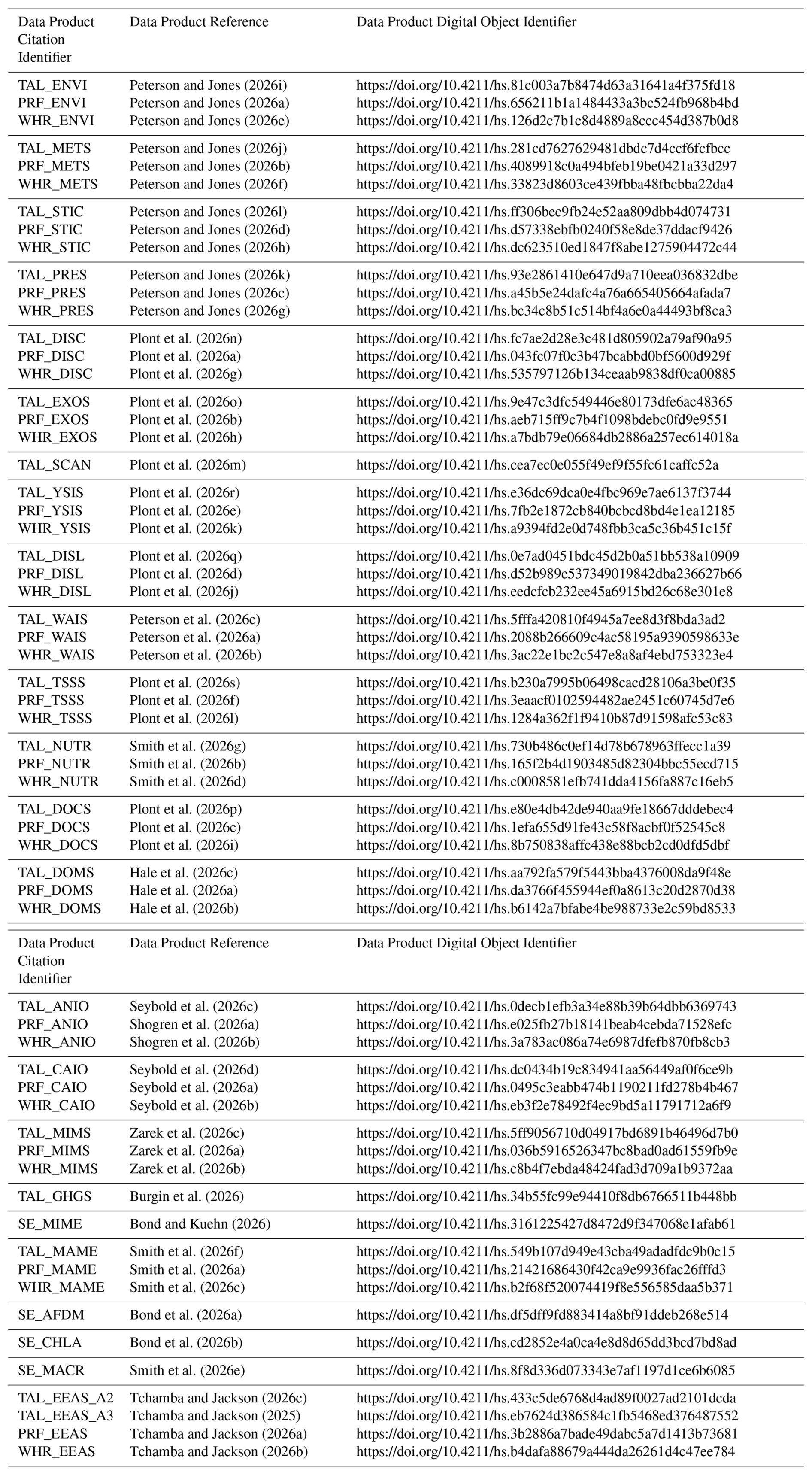
Table A2 Summary of hydrolytic and oxidative extracellular enzyme activities assessed in this study and their associated model substrates, assessed products, and descriptions of specific reactions.

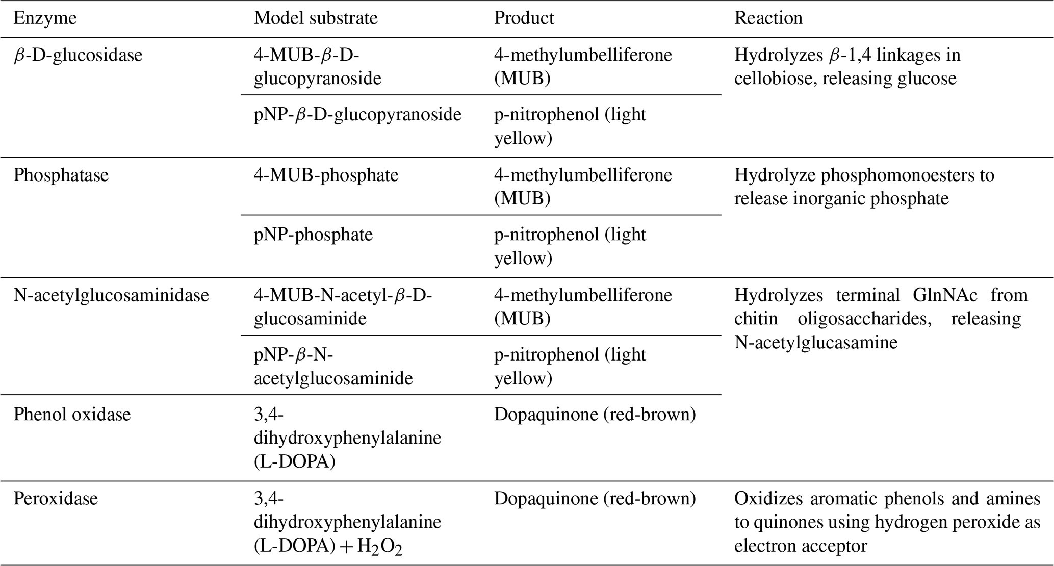
Table A3 National Center for Biotechnology Information Sequence Read Archive (NCBI SRA) accession numbers for 16S and ITS sequencing data products.

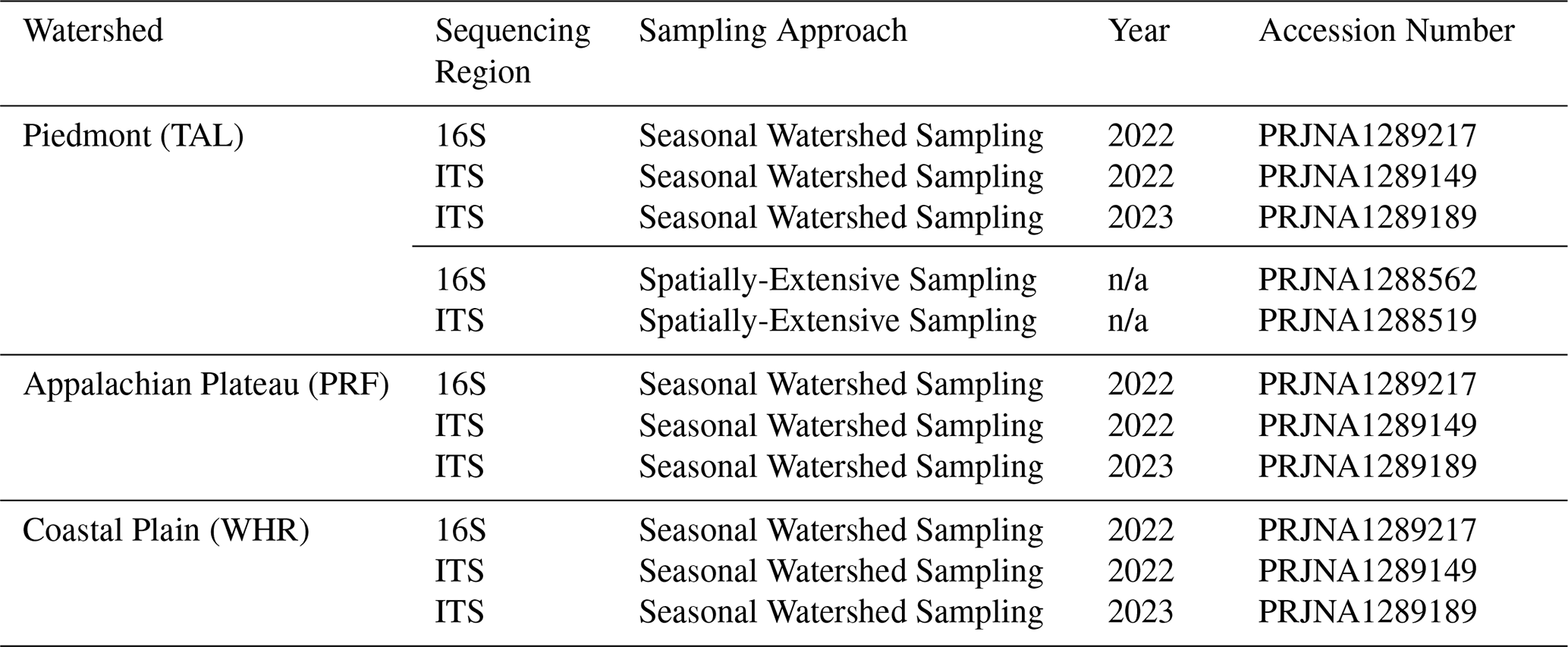
n/a – not applicable.