A global dataset of δ¹³C-CH₄ source signatures and associated uncertainties (1998–2022), with a sensitivity analysis to support isotopic inversions

The isotopic composition of atmospheric methane (δ¹³C-CH₄) provides critical constraints for attributing methane emissions to specific sources. In this study, we present updated global maps of δ¹³C-CH₄ source signatures across five major methane-emitting sectors (fossil fuels and geological, agriculture and waste, biomass and biofuel burning, wetlands, and other natural sources) for the period 1998–2022. These maps integrate recent spatially explicit datasets and literature-derived observations, and include explicit quantification of both intrinsic (within-sector) and aggregation-related uncertainties. Building upon previous global compilations, our dataset extends the temporal coverage to 2022, harmonizes sectoral definitions with the Global Methane Budget framework, and provides a consistent and traceable quantification of uncertainties suitable for atmospheric inversions. We assess the influence of these updated source signatures on the modeled atmospheric δ¹³C-CH₄ using forward simulations within the Community Inversion Framework (CIF) coupled to the LMDz transport model. A comprehensive sensitivity analysis quantifies the impacts of key drivers of uncertainty, including emission flux datasets, OH sinks, kinetic isotope effects, and isotopic source signatures. We show that uncertainties in methane oxidation chemistry and source signatures, particularly from agriculture and waste, dominate the variability in the modeled δ¹³C-CH₄ signal, while the impact of flux aggregation choices is comparatively minor. The updated isotopic dataset is provided on a global 1°×1° grid, supporting future atmospheric inversions and improved methane budget assessments at global and regional scales. Practical guidelines for configuring isotopic inversions, including recommended uncertainty specifications and key parameters to optimize, are also provided, offering a framework for next-generation δ¹³C-CH₄ inversion studies. The final version of the gridded δ¹³C-CH₄ source signature dataset is available under CC BY 4.0 (Tapin et al., 2025, https://doi.org/10.57780/ESA-6D202E9).

1 Introduction

Methane (CH₄) is the second most significant anthropogenic greenhouse gas after carbon dioxide (CO₂), playing a major role in current climate change (Stocker, 2014; Forster et al., 2023). Its atmospheric concentration has more than doubled since pre-industrial times, to reach 1946 ppb in November 2025 (Forster et al., 2023; Lan et al., 2026). Despite its lower abundance compared to CO₂, CH₄ has contributed approximately 31 % (1.19 W m⁻²) of the total radiative forcing from anthropogenic greenhouse gases since 1750 (Forster et al., 2023), owing to its high global warming potential (GWP: 29.8 over 100 years, 82.5 over 20 years). Its relatively short atmospheric lifetime (about 9 years for the burden; Prather et al., 2012, and approximately 12 years for the perturbation lifetime Forster et al., 2023) compared to CO₂ makes it an effective target for near-term climate mitigation strategies (Ocko et al., 2021; Shindell et al., 2021). Global initiatives such as the Global Methane Pledge (launched at COP26) aim to reduce global anthropogenic methane emissions by 30 % by 2030 compared to 2020 levels (Global Methane Pledge, 2023; UNEP and Climate and Clean Air Coalition, 2022). After a stabilization phase between 1999–2006, atmospheric CH₄ resumed its growth after 2007, diverging from trajectories compatible with the Paris Agreement (Nisbet et al., 2019). This renewed increase remains a subject of active scientific debate (Schwietzke et al., 2016; Schaefer et al., 2016; Nisbet et al., 2016, 2019; Rigby et al., 2017; Saunois et al., 2017; Worden et al., 2017; McNorton et al., 2018; Thompson et al., 2018; Schaefer, 2019; Turner et al., 2019; Fujita et al., 2020; Zimmermann et al., 2020; Jackson et al., 2020; Basu et al., 2022; Chandra et al., 2024; Thanwerdas et al., 2024; Fujita et al., 2025; Riddell-Young et al., 2025), and highlights the urgent need to better constrain methane sources and sinks (e.g. Saunois et al., 2017, 2020, 2025). Since 2020, the growth of atmospheric CH₄ has further accelerated, with unprecedented annual increases recorded between 2020–2022 (Michel et al., 2024; Jackson et al., 2024; Ciais et al., 2026).

Methane emissions have both natural (around 200 Tg CH₄ yr⁻¹, e.g. wetlands, freshwaters, geological sources, natural wildfires) and anthropogenic origins (around 320 Tg CH₄ yr⁻¹, e.g. agriculture, fossil fuel, waste, and anthropogenic biomass and biofuel burning) (Saunois et al., 2025). However, large uncertainties persist in the relative contributions of these sources. CH₄ fluxes can be estimated using two main approaches: bottom-up and top-down methods. Bottom-up methods use either emission inventories derived from sectoral activity data and emission factors, or process-based models (Saunois et al., 2025). While they offer detailed source-level information, these estimates are not directly constrained by atmospheric observations and often lead to budgets that are inconsistent with the atmospheric CH₄ burden. In contrast, top-down methods rely on atmospheric measurements of CH₄, including in situ observations from ground-based stations and remote sensing data from satellites, combined with transport models (e.g. LMDZ) to statistically optimize emissions. These approaches are global and observation-based but often struggle to attribute emissions to specific sources when those are co-located or have overlapping temporal signals (Houweling et al., 2017; Bergamaschi et al., 2018). They can also face regional attribution challenges, particularly in areas with sparse or uneven observational coverage (Saunois et al., 2020, 2025). The discrepancies between these two methods, in both magnitude and spatial distribution, highlight major gaps in our understanding of CH₄ sources and sinks (Saunois et al., 2025). Accurately attributing atmospheric CH₄ to specific formation processes can be difficult, especially when co-located sources cannot be differentiated using CH₄ mixing ratios or their spatial and seasonal variability (Bergamaschi et al., 2010, 2013; Kirschke et al., 2013; Saunois et al., 2017). Yet the quantification of individual methane sources is required to implement effective mitigation strategies.

The isotopic composition of methane, particularly the ratio of ¹³C to ¹²C, can be used for source attribution because it depends on the formation pathway (e.g. Sherwood et al., 2017; Lan et al., 2021b). It is expressed as δ¹³C-CH₄:

$$\begin{array}{}\text{(1)}& {\displaystyle }{\displaystyle }\mathit{\delta }{}^{\mathrm{13}}\mathrm{C}\text{-}{\mathrm{CH}}_{\mathrm{4}}=\left({\displaystyle \frac{{\left({}^{\mathrm{13}}\mathrm{C}{/}^{\mathrm{12}}\mathrm{C}\right)}_{\text{sample}}}{R_{\text{VPDB}}}}-\mathrm{1}\right)\times \mathrm{1000},\end{array}$$

where $\left({}^{\mathrm{13}}\mathrm{C}{/}^{\mathrm{12}}\mathrm{C}\right)$ denotes the ratio of molar quantities of ¹³C to ¹²C in the sample, and $R_{\text{VPDB}}=\mathrm{1.1113}\times {\mathrm{10}}^{-\mathrm{2}}$ is the ${}^{\mathrm{13}}\mathrm{C}/{}^{\mathrm{12}}\mathrm{C}$ ratio of the Vienna Pee Dee Belemnite (VPDB) reference material (Dunn et al., 2024; Camin et al., 2025).

Different CH₄ sources exhibit characteristic δ¹³C-CH₄ signatures due to their formation processes. Microbial sources (e.g. wetlands, ruminants) typically emit methane that is strongly depleted in ¹³C, with values ranging from −65 ‰ to −55 ‰ (Sherwood et al., 2017, 2021). Geographic variability in livestock emissions reflects differences in plant diets, specifically between C₃ plants (e.g. wheat, rice, trees) and C₄ plants (e.g. maize, sugarcane, tropical grasses), which have distinct carbon isotope compositions (Lan et al., 2021a). Wetland signatures also vary spatially, with more depleted values observed in boreal regions compared to tropical zones (Ganesan et al., 2018; Douglas et al., 2021; Oh et al., 2022). Fossil fuel-related variability can be large, driven by geological origin and processing techniques, with δ¹³C-CH₄ signatures spanning from −55 ‰ to −30 ‰ (Sherwood et al., 2017; Milkov and Etiope, 2018). Geological emissions may also reflect a diversity of geochemical processes, including both thermogenic and microbial pathways, leading to a broader range of δ¹³C-CH₄ signatures (Sherwood et al., 2017; Etiope et al., 2019). Pyrogenic sources (e.g. biomass and biofuel burning) are enriched in ¹³C, with values ranging from −25 ‰ to −15 ‰ (Sherwood et al., 2017, 2021), depending on the dominant vegetation type (C₃ or C₄) (Still et al., 2003; Randerson et al., 2012; Lan et al., 2021a). In addition to source-specific isotopic signatures, atmospheric sinks also fractionate methane isotopes through the Kinetic Isotope Effect (KIE). Lighter isotopologues (¹²CH₄) react faster with major oxidants such as OH, Cl, and O(¹D) than their heavier counterparts (¹³CH₄), leading to ¹³C enrichment in the remaining methane. This process alters the isotopic composition of atmospheric CH₄ signal compared to the original source-weighted average signatures.

Over the past two decades, a decreasing trend in atmospheric δ¹³C-CH₄ has been observed alongside increasing CH₄ concentrations (Nisbet et al., 2023; Michel et al., 2024; Schuldt et al., 2024, 2025). This anti-correlation suggests shifts in source contributions, sink processes, or both, providing additional constraints for methane budget reconstructions. Measurements of δ¹³C-CH₄ are increasingly integrated into atmospheric inversions to differentiate methane sources through their isotopic signatures (Schwietzke et al., 2016; Lan et al., 2021a). Such data help distinguish co-located or seasonally overlapping sources, assess sectoral contributions, and improve the accuracy of global and regional methane budgets. However, the global network of in situ δ¹³C-CH₄ measurements remains sparse, resulting in limited spatial coverage and hampering the characterization of regional isotopic gradients. This motivates the exploration of satellite-based retrievals of isotopic methane, which could substantially enhance global coverage. Feasibility studies using instruments such as GOSAT, TROPOMI, and Sentinel-5/UVNS have demonstrated the potential of remote sensing for δ¹³C-CH₄ observations (Malina et al., 2018, 2019). Recent inversion studies have already begun incorporating δ¹³C-CH₄ observations from surface networks (e.g. Fujita et al., 2020, 2025; Basu et al., 2022; Drinkwater et al., 2023; Thanwerdas et al., 2024), paving the way for future applications that jointly exploit surface and satellite isotopic constraints. However, further studies are needed to properly evaluate possible use of satellite-based isotopic observations in inversions as retrieval uncertainties remain large.

A prerequisite for such isotopic inversions is the availability of spatially explicit source signature maps and associated uncertainties. Existing datasets include contributions from Ganesan et al. (2018), Chang et al. (2019), Etiope et al. (2019), Sherwood et al. (2017, 2021), Lan et al. (2021a), Oh et al. (2022), and Menoud (2022). However, limitations remain, particularly in representing uncertainties and covariance structures of isotopic priors (Basu et al., 2022; Thanwerdas et al., 2024). Full sensitivity analyses are also needed to assess the robustness of inversion results with respect to isotopic assumptions (Thanwerdas et al., 2022b).

In this study, we present updated spatially explicit δ¹³C-CH₄ source signature maps, with associated uncertainty estimates, to support global and regional methane inversions. Our main objectives are to:

• i.

  improve prior knowledge of isotopic compositions for major CH₄ sectors and subsectors,

• ii.

  evaluate the influence of the revised maps on modeled atmospheric δ¹³C-CH₄ using forward simulations,

• iii.

  quantify the sensitivity of modeled δ¹³C-CH₄ to key parameters and regions, and

• iv.

  provide uncertainty estimates and recommendations for integrating isotopic constraints into inversion frameworks.

Rather than validating the updated source signature maps against atmospheric observations, the sensitivity analysis focuses on quantifying the impact of key sources of uncertainty on modeled atmospheric δ¹³C-CH₄ distributions. This sensitivity-centered approach allows us to identify the dominant drivers of variability in the modeled isotopic signal and to provide practical recommendations for future inversion studies. Model-data comparisons, while essential, are beyond the scope of this work and will be addressed in subsequent studies.

The structure of the paper is as follows. Section 2 describes the development of the updated δ¹³C-CH₄ source signature maps. Section 3 presents the atmospheric modeling framework used for the sensitivity analysis. Section 4 reports and discusses the main results.

2 Development of updated δ¹³C-CH₄ source signature maps

To improve the spatial and temporal representation of isotopic methane emissions in inverse modeling, we developed a comprehensive set of global maps representing the δ¹³C-CH₄ source signatures across major methane-emitting sectors and sub-sectors, covering the period 1998–2022. The dataset is available at the ESA Open Science Data portal: (Tapin et al., 2025, https://doi.org/10.57780/ESA-6D202E9). These maps have a spatial resolution of 1°×1° (global coverage) and a monthly time step, providing improved temporal representation and either matching or improving the spatial resolution of previous datasets. It is based on a synthesis of recent gridded data products and regional observations from peer-reviewed literature (Sect. 2.1). The resulting dataset distinguishes five primary source sectors: fossil fuel exploitation and geological (FFG), agriculture and waste (AGW), biomass and biofuel burning (BB), wetlands (WET), and other natural sources (NAT), each composed of multiple underlying sub-sectors detailed (Sect. 2.2). The associated uncertainties were also calculated (Sect. 2.3). The methodology presented in this section provides a reproducible and publicly available framework to generate δ¹³C-CH₄ source signature maps at global scale, including explicit quantification of associated uncertainties. All acronyms, sector names and dataset abbreviations used throughout this study are summarized in Table S1 in the Supplement for clarity.

2.1 Construction of sub-sector isotopic signature maps

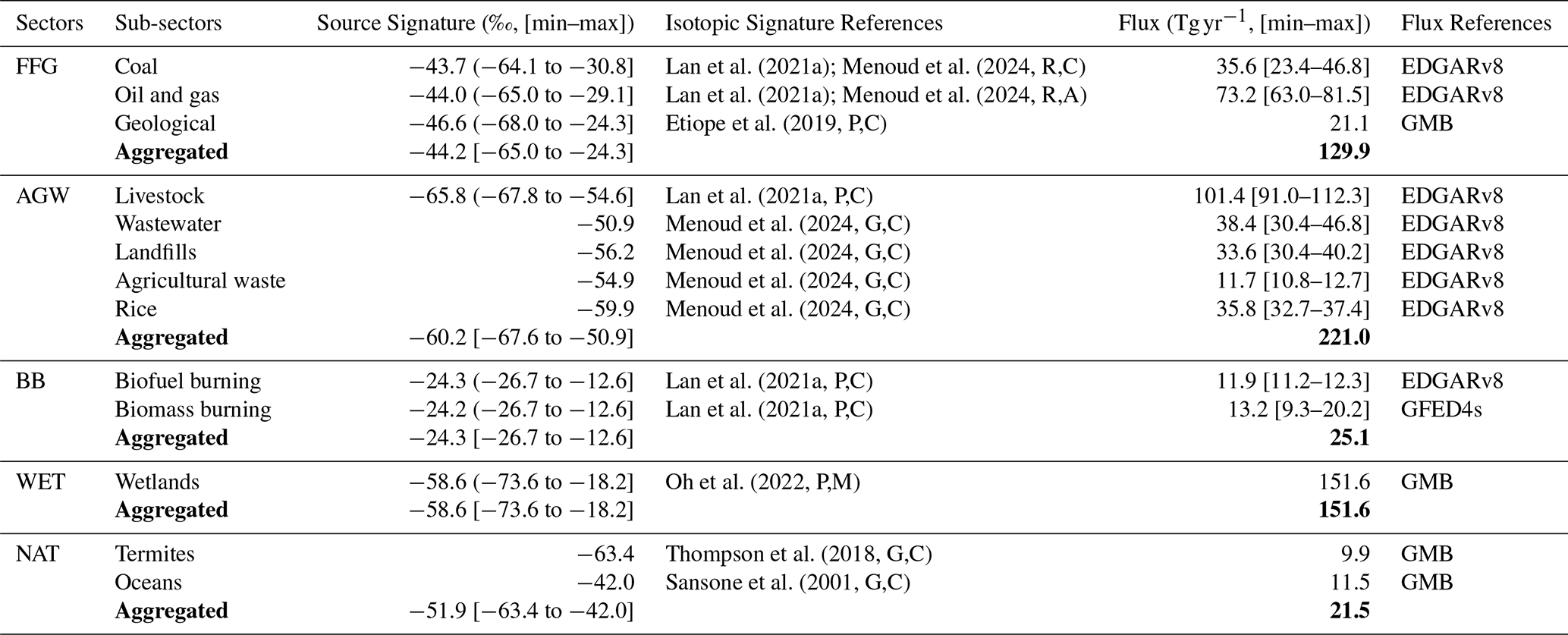
The construction of these maps relied on the integration of the most up-to-date isotopic datasets available for each methane source sub-sector. Table 1 provides an overview of the aggregated source sectors, their sub-sectors, the associated δ¹³C-CH₄ ranges, isotopic data sources, and corresponding emission fluxes. Gridded products were prioritized when available (e.g. Lan et al., 2021a; Oh et al., 2022), and were supplemented by regional datasets (e.g. Menoud et al., 2024) or literature-based estimates when spatially explicit data were lacking. To ensure representativeness at the global scale, a combination of pixel-level (P), regional (R), and global (G) datasets was used. The temporal resolution of the isotopic signatures was preserved when available in the source datasets, using annual (A) or monthly (M) variations. Otherwise, constant (C) values over the 1998–2022 period were assumed. Each entry in Table 1 is associated with metadata indicating its spatial (P, R, G) and temporal (C, A, M) resolution. All isotopic signatures are expressed relative to the VPDB standard; a discussion of the VPDB vs. historical PDB reference scales and their negligible impact on the simulations is provided in Sect. S1.1 in the Supplement. The following sections detail the specific methodologies applied to key source categories and describe how temporal or spatial gaps were addressed to produce a consistent, gridded isotopic dataset.

Lan et al. (2021a); Menoud et al. (2024, R,C)Lan et al. (2021a); Menoud et al. (2024, R,A)Etiope et al. (2019, P,C)Lan et al. (2021a, P,C)Menoud et al. (2024, G,C)Menoud et al. (2024, G,C)Menoud et al. (2024, G,C)Menoud et al. (2024, G,C)Lan et al. (2021a, P,C)Lan et al. (2021a, P,C)Oh et al. (2022, P,M)Thompson et al. (2018, G,C)Sansone et al. (2001, G,C)

Table 1 Methane emission sectors aggregated for atmospheric modeling, including representative δ¹³C-CH₄ isotopic signatures and flux estimates over 1998–2022. For each major sector (FFG, AGW, BB, WET, NAT), sub-sectoral values are compiled and aggregated using flux-weighted averages. Isotopic signature ranges reflect observed variability within each sub-sector, based on available spatial and temporal resolution: (P) pixel-level, (R) regional, or (G) global data, and (C) constant, (A) annual, or (M) monthly data. Flux estimates are derived from the Emissions Database for Global Atmospheric Research (EDGARv8; Crippa et al., 2023), the Global Fire Emissions Database (GFED4s; van Wees et al., 2022), and the Global Methane Budget (GMB; Martinez et al., 2024). Bold font is used in the “Aggregated” rows to mark the flux-weighted sector-level values (both the aggregated δ¹³C-CH₄ source signature and the aggregated flux).

2.1.1 Treatment of European fossil fuel isotopic signatures

For fossil fuel emissions in Europe, regional measurements from the European Methane Isotope Database (EMID; Menoud et al., 2024) were combined with the global inventory from Lan et al. (2021a) to improve the spatial accuracy of isotopic signatures. The Lan et al. (2021a) dataset, based on the compilation by Sherwood et al. (2021), includes isotopic data from over 13 000 locations from 347 references, though it remains largely U.S. centered. The EMID database provides additional coverage, including both literature data and new measurements from the MEMO² project for fossil fuel sources over Europe (European Commission, 2017). The extended global database, combining EMID with Sherwood et al. (2021) and MEMO², consists of over 13 313 δ¹³C measurements from 64 countries.

The integration of these two datasets was conducted as follows:

1. Country-level average δ¹³C-CH₄ signatures were computed from EMID for some European countries (e.g. UK, Germany, Poland, Romania, France), corresponding to those for which data are available in the EMID inventory.

2. These averages were then combined with Lan et al. (2021a) data using a weighting factor that accounts for the number of additional observations in EMID compared to Sherwood et al. (2021) dataset.

The resulting aggregated values are presented in Table S2 in the Supplement.

2.1.2 Temporal extrapolation

To ensure full temporal coverage over the 1998–2022 period, extrapolation was required for certain datasets whose original time series ended prematurely, specifically for the oil and gas and wetland sub-sectors. In both cases, specific strategies were applied based on known emission trends and isotopic characteristics of source signatures.

For the oil and gas sub-sector, the dataset from Lan et al. (2021a) ends in 2016. Post-2016 values were extrapolated only for U.S. data, based on documented trends in U.S. unconventional gas production (U.S. Energy Information Administration, EIA, https://www.eia.gov/energyexplained/us-energy-facts, last access: 14 March 2025), notably shale gas, which typically exhibits lighter δ¹³C-CH₄ signatures than conventional sources (Sherwood et al., 2017). Basin-level variability in both gas production and isotopic composition was accounted for using data from the EIA natural gas reports (https://www.eia.gov/naturalgas/weekly/, last access: 9 March 2025) and published isotopic measurements (Milkov et al., 2020b). Outside the U.S., signatures values were held constant. We adopted a two-step method to extrapolate U.S. δ¹³C-CH₄ values post-2016:

1. computing basin-weighted δ¹³C-CH₄ values based on production volumes, using shale gas data per basin (EIA, https://www.eia.gov/dnav/ng/ng_prod_shalegas_s1_a.html, last access: 9 March 2025) and basin-specific isotopic signatures (Milkov et al., 2020b);

2. adjusting national-scale δ¹³C-CH₄ values according to the evolving share of shale gas in total production (EIA, https://www.eia.gov/naturalgas/weekly/, last access: 9 March 2025).

For wetlands, the monthly δ¹³C-CH₄ source signature maps from Oh et al. (2022) also end in 2016. To extend the dataset beyond this point, we extrapolated the 2016 seasonal cycle linearly and incorporated the long-term trend in source signatures of $-\mathrm{0.02}\mathrm{‰}{\mathrm{yr}}^{-\mathrm{1}}$ observed over the 1984–2016 period (Oh et al., 2022).

2.2 Aggregation into source sectors

To facilitate the integration of δ¹³C-CH₄ source signatures into atmospheric modeling and to optimize computational efficiency, detailed source sub-sectors were aggregated into broader emission sectors using flux-weighted mean values (more details in Sect. S1.2 in the Supplement). This aggregation preserves the key isotopic characteristics of different emission types while reducing model complexity. The classification follows the methodology adopted in the Global Methane Budget (GMB Saunois et al., 2025), grouping methane emissions into five principal source categories (Table 1):

• FFG includes emissions from oil, gas, coal, industrial activities, transport, and natural geological seepage.

• AGW encompasses emissions from enteric fermentation, rice cultivation, manure management, and waste decomposition.

• BB sector comprises emissions from open biomass combustion and biofuel use.

• WET includes natural wetland emissions as well as emissions from freshwater systems such as lakes, ponds, reservoirs, rivers, and streams.

• NAT sector covers natural non-wetland emissions, including mostly those from termites and oceanic sources.

This aggregation aims to ensure isotopic representativity within each sector, in line with recent recommendations for source signature consistency (Mannisenaho et al., 2023). An exception may apply to the NAT sector, which encompasses heterogeneous processes (e.g. termite emissions vs. oceanic sources) that are not co-located. These sub-sources were grouped primarily due to their relatively small fluxes and to limit the number of categories for computational efficiency, rather than based on isotopic or spatial consistency. A comprehensive mapping between detailed subcategories and the aggregated sectors used in this study is provided in Table 1. In cases where isotopic data were missing for a specific pixel, flux-weighted average values were used so that each sector's data covered the entire domain.

Both the aggregated maps for the five main source sectors and the underlying maps for the 14 sub-sectors listed in Table 1 are publicly distributed (see Code and data availability). This dual format allows users to either directly use the inversion-ready aggregated product, or to re-aggregate the sub-sector maps using their own flux-weighting scheme, sectoral classification, or extended sub-sector breakdown if their inversion framework requires a finer or different grouping.

2.3 Uncertainty assessment of aggregated source signatures

This section describes how uncertainties in aggregated δ¹³C-CH₄ source signatures are estimated. All uncertainties are evaluated at the global scale, i.e. they are not spatially resolved at the grid-cell level. The overall propagation pathway, from sub-sector measurements to inversion error structures, is summarized schematically in Fig. 1. In what follows, we describe the three components of this propagation chain: the total uncertainty σ_total combining all contributions (Sect. 2.3.1), the propagated uncertainty σ_prop derived from sub-sector variability (Sect. 2.3.2), and the aggregation uncertainty σ_agg reflecting inventory choices (Sect. 2.3.3).

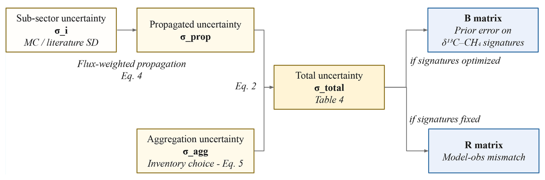
Figure 1 Schematic overview of the uncertainty propagation pathway for δ¹³C-CH₄ source signatures. Sub-sector isotopic uncertainties (σ_i), derived from Monte Carlo simulations (lower bound) and literature standard deviations (upper bound), are propagated to the sector level (σ_prop) via flux-weighted error propagation (Eq. 4). The aggregation uncertainty (σ_agg), estimated from sensitivity tests using different emission inventories (Eq. 5), is combined with σ_prop to yield the total sectoral uncertainty (σ_total, Eq. 2). In atmospheric inversion frameworks, σ_total informs either the prior error covariance matrix (B) if isotopic source signatures are optimized, or the observation error covariance matrix (R) if they are held fixed (see Sect. 4.3.2).

2.3.1 Total uncertainty (σ_total)

To quantify the uncertainty associated with the aggregated δ¹³C-CH₄ source signatures (σ_total), we consider two main components: (i) the propagated uncertainty from sub-sector level to sector level (σ_prop), i.e. the intrinsic isotopic uncertainty from sub-sector, and (ii) the aggregation uncertainties (σ_agg), i.e. the variability introduced when aggregating sub-sector signatures into sector-level values, using a given set of flux weights from prior inventories. Assuming that the two types of uncertainties are independent, the total uncertainty for each aggregated sector is calculated by combining these two components:

$$\begin{array}{}\text{(2)}& {\displaystyle }{\displaystyle }{\mathit{\sigma }}_{\text{total}}=\sqrt{{\mathit{\sigma }}_{\text{prop}}^{\mathrm{2}}+{\mathit{\sigma }}_{\text{agg}}^{\mathrm{2}}}\end{array}$$

The corresponding relative uncertainty (in percentage) is then calculated as:

$$\begin{array}{}\text{(3)}& {\displaystyle }{\displaystyle }\text{Relative uncertainty (\%)}=\left({\displaystyle \frac{{\mathit{\sigma }}_{\text{total}}}{\left|\stackrel{\mathrm{‾}}{{\mathit{\delta }}^{\mathrm{13}}{\mathrm{C}}_{\text{sector}}}\right|}}\right)\times \mathrm{100}\end{array}$$

where σ_prop corresponds to the propagated uncertainty at the sector level derived from sub-sector uncertainties (‰), σ_agg represents the uncertainty associated with the aggregation method, estimated from sensitivity tests (‰) and $\stackrel{\mathrm{‾}}{{\mathit{\delta }}^{\mathrm{13}}{\mathrm{C}}_{\text{sector}}}$ denotes the mean isotopic signature of the aggregated sector (‰).

Because the propagated uncertainty σ_prop is provided as a range, the resulting total uncertainty σ_total is also expressed as a corresponding range rather than a single value.

2.3.2 Propagated uncertainty from sub-sectors (σ_prop)

The term σ_prop represents the propagated uncertainty from sub-sector isotopic composition (σ_i) to the aggregated sector level. First, the isotopic uncertainty for each sub-sector (σ_i) is estimated using two complementary approaches, depending on the origin of the data:

• The standard deviations of δ¹³C-CH₄ values reported in the literature, using the dataset compiled by Menoud et al. (2022), which captures spatial variability and methodological dispersion;

• The uncertainty values reported by Lan et al. (2021a), who derived them from 10 000 Monte Carlo simulations at the grid-cell level, explicitly propagating measurement and modeling errors through source attribution and mixing processes.

The Monte Carlo approach provides a precise uncertainty estimate directly linked to sub-sector diversity but may underestimate broader, large-scale variability and inter-regional differences. Conversely, the literature-based standard deviation offers a more conservative benchmark that captures additional inter-study, regional, and methodological variability. The two approaches (literature-based standard deviations and Monte Carlo uncertainties) provide lower and upper estimates of the sub-sector isotopic uncertainty.

Second, the sub-sector uncertainties (σ_i) are propagated into the aggregated sector uncertainty component (σ_prop) using a flux-weighted error propagation approach:

$$\begin{array}{}\text{(4)}& {\displaystyle }{\displaystyle }{\mathit{\sigma }}_{\text{prop}}=\sqrt{\sum _i{\left({\displaystyle \frac{F_i}{F_{\text{total}}}}\right)}^{\mathrm{2}}{\mathit{\sigma }}_i^{\mathrm{2}}}\end{array}$$

where F_i is the flux of sub-sector i (Tg yr⁻¹), F_total is the total flux of the aggregated sector (Tg yr⁻¹), and σ_i is the isotopic uncertainty of sub-sector i (‰).

The aggregated sector uncertainty (σ_prop) is reported as a range, with the lower bound corresponding to the Monte Carlo estimate and the upper bound corresponding to the literature-based estimate.

2.3.3 Aggregation uncertainty (σ_agg)

This component reflects the sensitivity of aggregated signatures to methodological choices of weighting fluxes in the construction of the aggregated sector dataset. It is evaluated through a series of sensitivity tests (see Sect. 4.2), and computed as the standard deviation across the resulting aggregation scenarios:

$$\begin{array}{}\text{(5)}& {\displaystyle }{\displaystyle }{\mathit{\sigma }}_{\text{agg}}=\sqrt{{\displaystyle \frac{\mathrm{1}}{N}}\sum _{j=\mathrm{1}}^N({\overline{x}}_j-\overline{x}{)}^{\mathrm{2}}}\end{array}$$

where ${\overline{x}}_j$ is the mean isotopic signature derived from aggregation method j, $\overline{x}$ is the overall mean isotopic signature across all tested methods, and N is the number of tested aggregation methods.

In summary, this framework provides consistent tools to estimate sectoral δ¹³C-CH₄ uncertainties, combining sub-sector variability and aggregation effects. Beyond sectoral aggregation, isotopic uncertainties also carry a latitudinal dimension, driven notably by the distribution of C₃ and C₄ plants across source sectors and by stratospheric transport processes; these spatial gradients are discussed further in Sect. 4.1.1. Because uncertainties in isotopic signature values and their spatial allocation propagate into regional and global inversions, ultimately influencing source attribution, it is particularly important to assess them. The resulting uncertainties are directly usable in atmospheric models and inversions to inform prior error structures and guide optimization choices (see Sect. 4.3.2).

3 Atmospheric framework for sensitivity analysis

Building on recent flux inventories and isotopic signature datasets, we developed updated δ¹³C-CH₄ source signature maps suitable for atmospheric modeling and inversion studies (see Sect. 2). This section presents how these maps are integrated into forward atmospheric simulations to assess how key parameters uncertainties propagate to the modeled δ¹³C-CH₄ signal. We first describe the modeling framework used for the simulations (Sect. 3.1), then detail the sensitivity experiments designed to explore the influence of critical drivers, including methane fluxes, fluxes used for isotopic aggregation, OH fields, OH kinetic isotope effects, and isotopic source signatures (Sect. 3.2).

3.1 Description of atmospheric simulations

To assess the influence of key parameters and evaluate the impact of the updated δ¹³C-CH₄ signature dataset, we conducted a sensitivity analysis based on forward simulations of methane mole fractions and δ¹³C-CH₄ signals over the period 1998–2022. These simulations were performed within the Community Inversion Framework (CIF; Berchet et al., 2021). The CIF was extended by Thanwerdas et al. (2022a) to incorporate isotopic constraints, enabling the joint simulation and assimilation of CH₄ mole fractions and their δ¹³C-CH₄ composition. The following subsections describe in detail all components of the forward simulations.

3.1.1 Global transport model

The simulations were conducted using the LMDz transport model, a component of the coupled model from the Institut Pierre-Simon Laplace (IPSL-CM), developed at the Laboratoire de Météorologie Dynamique (LMD; Hourdin et al., 2006). The offline version was used, driven by ECMWF ERA-Interim reanalyses, as described in Chevallier et al. (2005). LMDz operates at a horizontal resolution of 3.75°×1.875°, with 39 vertical hybrid sigma-pressure levels extending up to approximately 75 km. The model time step is 30 min. Vertical diffusion is parameterized following the local approach of Louis (1979), while deep convection is represented using the Kerry Emanuel scheme (Remaud et al., 2018).

3.1.2 Emissions fluxes

Source categories are described in Table 1 with the following emission fluxes: All flux datasets were selected to ensure consistency with the Global Methane Budget (GMB) framework (Saunois et al., 2020, 2025), which provides the reference basis for methane emission assessments.

• Anthropogenic sources. Emissions from agriculture, waste, fossil fuel exploitation, and biofuel combustion are taken from the EDGARv8 inventory (Crippa et al., 2023). This dataset provides detailed activity data and region-specific emission factors, enabling realistic representation of spatial and temporal variability across sectors and regions.

• Biomass burning. Emissions from wildfires and agricultural burning are derived from the Global Fire Emissions Database (GFED4s) (van Wees et al., 2022). GFED4s integrates satellite observations of burned area, fire radiative power, and biogeochemical model outputs to provide monthly CH₄ flux estimates.

• Wetlands. Wetland emissions are estimated using the multi-model mean of 11 process-based models compiled within the Global Methane Budget framework (Martinez et al., 2024). These fluxes are provided as monthly climatological values.

• Freshwater systems. Emissions from lakes and reservoirs are based on the CH₄ flux maps by Stavert et al. (2022). Initial global emissions are estimated at 95 Tg yr⁻¹, reduced to 73 Tg yr⁻¹ after ice-cover corrections. Following Martinez et al. (2024), emissions are further rescaled by a factor of one-third, resulting in a global total of 53 Tg yr⁻¹ (Saunois et al., 2025). We acknowledge that freshwater flux estimates remain subject to large uncertainties, arising from poorly mapped inland water extent, complex emission pathways, and spatial variability in methanotrophy (e.g. Van Bergen et al., 2019; Lauerwald et al., 2023; Shaw et al., 2022). These uncertainties are further discussed in Sect. 4.2.2.

• Termites. Termite emissions follow Martinez et al. (2024) based on the S. Castaldi model, providing a spatially explicit global climatology without accounting for seasonal variability.

• Geological methane. Geological emissions use the gridded climatology from Etiope et al. (2019), rescaled to a total global flux of 21 Tg CH₄ yr⁻¹ by Martinez et al. (2024). Offshore geological emissions, including marine seepage, are excluded to avoid double counting. We note that geological emission estimates remain uncertain; ice core-based constraints suggest that pre-industrial geological emissions may have been substantially lower (Petrenko et al., 2017), though the current value follows the Global Methane Budget framework (Martinez et al., 2024) for consistency with the broader modeling setup.

• Oceanic methane. Ocean emissions rely on the climatological dataset of Weber et al. (2019), which combines microbial CH₄ production in the water column and geological seepage from seafloor sediments. These emissions are considered seasonally invariant and included as a static component of the total CH₄ flux budget (Martinez et al., 2024).

3.1.3 Initial conditions

Initial conditions for CH₄ and δ¹³C-CH₄ for the year 1998 were derived from an inversion covering the period 1988–2020 (Thanwerdas et al., 2024). A spin-up period from 1998 to 2016 was used to allow the model to adjust to realistic atmospheric gradients, particularly for δ¹³C-CH₄ (Tans, 1997). Only the period 2016–2020 is analyzed to ensure that the model has reached a stable state and to enable direct comparison between simulations, which differ only from the perturbed parameters (see Sect. 3.2).

3.1.4 Chemistry

Methane oxidation is simulated using the generic chemical module of the offline LMDz model (Pison et al., 2009; Thanwerdas et al., 2022b). The chemical scheme includes reactions with hydroxyl radicals (OH), excited atomic oxygen (O(¹D)), and chlorine radicals (Cl). Oxidant concentrations are prescribed from precomputed daily 3-D fields summarized in Table 2.

• Hydroxyl radicals (OH). OH is the primary sink for atmospheric methane. Monthly mean OH fields are taken from LMDz-INCA simulations (Hauglustaine et al., 2004), driven by consistent meteorological forcing with the transport model.

• Excited atomic oxygen (O(¹D). O(¹D) contributes mainly to methane oxidation in the stratosphere. A monthly climatology from the TRANSCOM project (Patra et al., 2011) is used.

• Chlorine radicals (Cl). Methane destruction by Cl radicals is particularly relevant in both the marine boundary layer and the stratosphere. Cl fields are based on the dataset of Wang et al. (2021), as recommended by Thanwerdas et al. (2022b), and include both tropospheric and stratospheric concentrations.

Saueressig et al. (2001)(Hauglustaine et al., 2004)Saueressig et al. (2001)(Patra et al., 2011)Saueressig et al. (1995)Wang et al. (2021)

Table 2 Fractionation coefficients for methane oxidation reactions with OH, O(¹D), and Cl. The kinetic isotope effect (KIE) values are shown for each reaction, along with their respective references and sources of the 3D oxidant fields. For Cl, the KIE is expressed as a temperature-dependent exponential function, where T denotes temperature in Kelvin (K).

Isotopic fractionation from CH₄ oxidation is expressed by the kinetic isotope effects (KIEs), which quantify the difference in reaction rates between ¹²CH₄ and ¹³CH₄. The KIE values used for each oxidant are summarized in Table 2. A sensitivity analysis is conducted on the OH-KIE value, given its significant impact on the atmospheric δ¹³CH₄ signal (see Sect. 3.2).

3.1.5 Soil sink

Soil uptake is a significant sink for atmospheric methane, and accounts for approximately 35 Tg CH₄ yr⁻¹ in the global methane budget (Saunois et al., 2025). Moreover, the soil sink is known to induce isotopic fractionation, which must be accounted for in forward simulations of the isotopic signal (Snover and Quay, 2000). In this study, rather than using a fixed negative flux, we represent soil uptake as a first-order deposition process, where the deposition velocity v_dep is computed from prescribed soil fluxes and modeled surface CH₄ concentrations. This approach allows the sink to respond to atmospheric gradients and enables a consistent application of isotopic fractionation. Representing soil uptake via a deposition velocity ensures that the isotopic fractionation is applied dynamically to both ¹²CH₄ and ¹³CH₄, in proportion to their atmospheric concentrations and the kinetic isotope effect.

The monthly deposition velocity is calculated as:

$$\begin{array}{}\text{(6)}& {\displaystyle }{\displaystyle }{v}_{\text{dep}}={\displaystyle \frac{F_{\text{soil}}}{C_{{\text{CH}}_{\mathrm{4}}}}}\end{array}$$

where F_soil is the prior soil uptake flux from the GMB dataset (Martinez et al., 2024), and $C_{{\text{CH}}_{\mathrm{4}}}$ is the modeled surface CH₄ mole fraction from inversion (Thanwerdas et al., 2024).

To account for isotopic fractionation during methane uptake by soils, a kinetic isotope effect (KIE) is applied. The deposition velocity for ¹³CH₄ is computed as:

$$\begin{array}{}\text{(7)}& {\displaystyle }{\displaystyle }{v}_{\text{dep},{}^{\mathrm{13}}{\text{CH}}_{\mathrm{4}}}={\displaystyle \frac{v_{\text{dep},{}^{\mathrm{12}}{\text{CH}}_{\mathrm{4}}}}{{\text{KIE}}_{{\mathit{\delta }}^{\mathrm{13}}\mathrm{C}}}}\end{array}$$

with a fractionation factor ${\text{KIE}}_{{\mathit{\delta }}^{\mathrm{13}}\mathrm{C}}=\mathrm{1.020}$, based on the experimental results of Snover and Quay (2000).

The methodology presented in this section provides a consistent framework for simulating atmospheric CH₄ mole fractions and δ¹³C-CH₄ signals using the CIF coupled to the LMDz transport model.

3.2 Protocol for sensitivity experiments

A series of sensitivity simulations was conducted to assess the impact of key input uncertainties on the modeled spatial and temporal variability of atmospheric δ¹³C-CH₄ signal and CH₄ mole fractions. The purpose of these sensitivity experiments and the way input and output uncertainties are propagated within the inversion framework are illustrated in Fig. 4. These experiments, summarized in Table 3, are grouped into four main categories:

• Flux aggregation. We tested the sensitivity of modeled outputs to the choice of emission inventories used for isotopic flux aggregation. Fluxes were aggregated using different anthropogenic inventories, namely the Emissions Database for Global Atmospheric Research (EDGARv8; Crippa et al., 2023), the Global Fuel Exploitation Inventory (GFEIv2; Scarpelli et al., 2022), the Community Emissions Data System (CEDSv2021; O'Rourke et al., 2021), and the Greenhouse Gas and Air Pollution Interactions and Synergies model (GAINSv4; Höglund-Isaksson et al., 2020). These datasets are collectively referred to as “inventories” hereinafter. We also tested the effect of increasing the number of aggregated source categories (from 5 to 14) to assess the trade-offs between computational efficiency and isotopic detail (see Sect. 2.2).

• Chemistry. Sensitivity to CH₄ oxidative loss processes was explored by using different OH fields, including the INCA model (Hauglustaine et al., 2004), the TRANSCOM-MCFCAL ensemble (Patra et al., 2011), and the IAV scenario (Patra et al., 2021), as well as by varying the kinetic isotope effects (KIEs) associated with CH₄ oxidation by OH radicals (Cantrell et al., 1990; Saueressig et al., 2001). Note that the other two CH₄ oxidation pathways included in the model, Cl oxidation and soil uptake, were not independently perturbed in the sensitivity ensemble. The impact of Cl fields on modeled CH₄ and δ¹³C-CH₄ within the same LMDz-SACS framework has been comprehensively quantified by Thanwerdas et al. (2022b), and we adopt here the Cl field from Wang et al. (2021). The soil sink, implemented as an isotope-sensitive first-order deposition process (Sect. 3.1.5), carries a well-constrained global magnitude and a moderate KIE. The implications of these two sinks for the δ¹³C-CH₄ budget are discussed in Sect. 4.2.3.

• CH₄ fluxes. Sensitivity to the choice of methane flux datasets was assessed for three sectors: wetlands (GMB climatology and interannual variability (IAV) (Martinez et al., 2024), LPJ from GMB (Saunois et al., 2020), SatWetCH₄ (Bernard et al., 2025)); freshwater systems (on/off configuration using GMB Martinez et al., 2024); and anthropogenic sources (EDGARv8, CEDSv2021, GAINSv4, GFEI).

• Isotopic signature. For the five main source sectors, a Monte Carlo ensemble (five members) was generated to isolate the influence of source signature uncertainties on the modeled δ¹³C-CH₄. Isotopic signatures were randomly perturbed within their sector-specific uncertainty ranges, assumed to follow normal distributions (see Sect. 4.1.3). Each spatial domain draws independently from this distribution, so that different regions may receive different perturbed values within the same Monte Carlo member. Further details, including the statistical parameters used for each sector, are provided in Table S3 in the Supplement.

Table 3 Overview of the simulation setups used for the sensitivity analysis. Simulations are grouped into three main categories (Category): chemistry, aggregation, and fluxes. The column Subcategory specifies the specific parameter being tested (e.g. OH fields, KIE values, wetland emissions, freshwater emissions, anthropogenic emissions). Simulation names in italic correspond to the reference simulations used in each category. Models and datasets used include: INCA (Hauglustaine et al., 2004), IAV (Patra et al., 2021), MCFCAL (Patra et al., 2011) for OH fields, Saueressig (Saueressig et al., 2001) and Cantrell (Cantrell et al., 1990) for OH kinetic isotope effects (KIE), EDGARv8 (Crippa et al., 2023), GFEI v2 (Scarpelli et al., 2022), CEDS v2021-04-21 (O'Rourke et al., 2021), and GAINSv4 (Höglund-Isaksson et al., 2020) for anthropogenic emissions, GMB (Martinez et al., 2024) for freshwater emissions, and various versions of wetland emissions from Saunois et al. (2020), including GMB_Mean (climatological mean of 11 models), GMB_NoClimato (monthly mean of 11 models), and LPJ (LPJ-wsl model). The bold font highlights, for each subcategory, the specific parameter value that is perturbed relative to the reference simulation (whose name is given in italic).

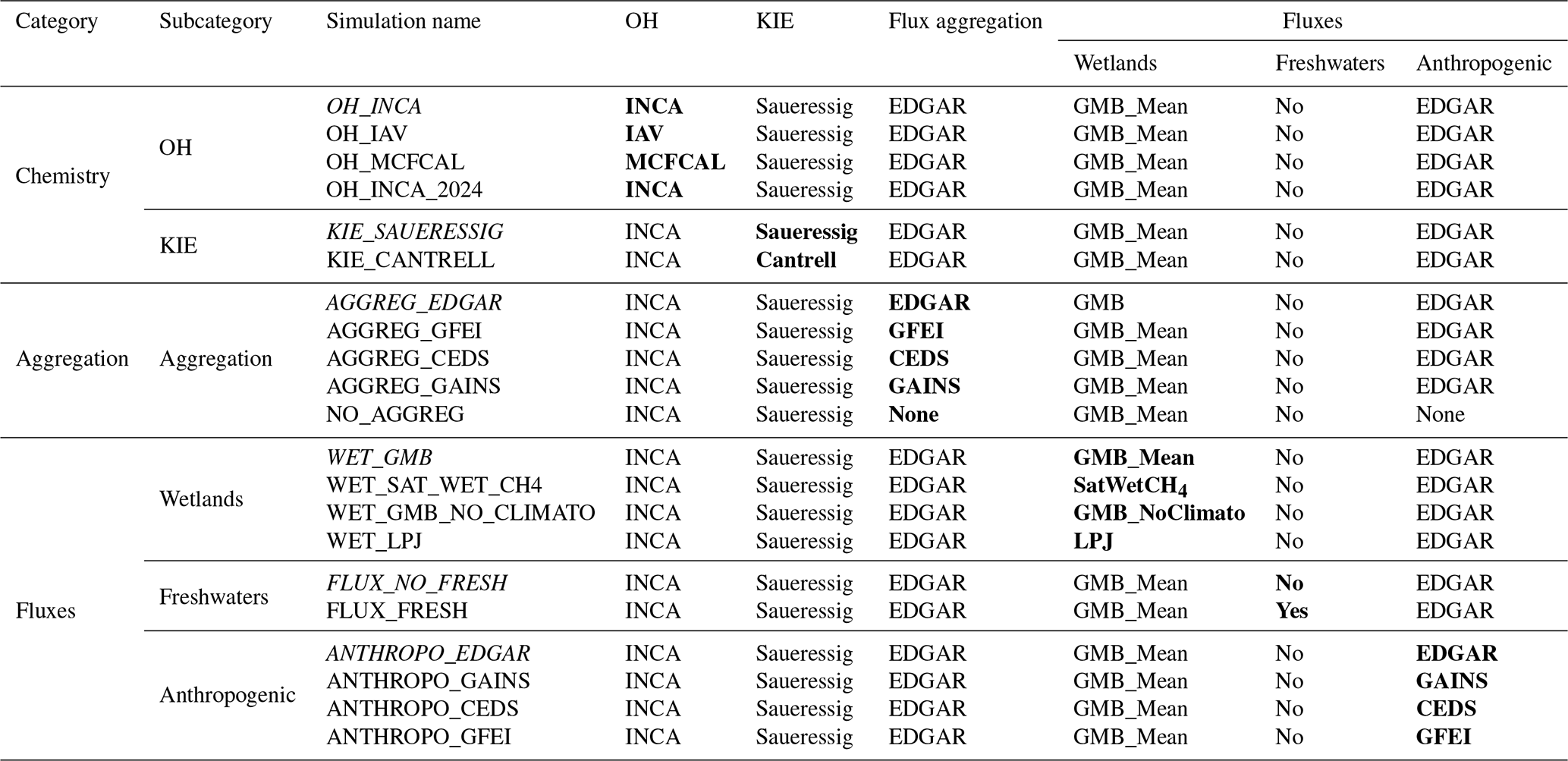
The sensitivity analysis focuses on the period from 2016 to 2020 included. The years from 1998 to 2015 are used as a spin-up period to let the model adjust, during which the simulated atmospheric CH₄ and δ¹³C-CH₄ progressively stabilize (see Sect. S4 in the Supplement for the full 1998–2022 time series of all simulations compared to NOAA-INSTAAR observations Michel et al., 2024; Schuldt et al., 2025). The simulation outputs from January 2016 to December 2020 are analyzed. The years 2021–2022 are excluded to ensure consistency across all simulations, as some of the emission inventories used (e.g. GAINS) are only available up to 2020. These simulations aim to quantify the uncertainties introduced by methodological choices during the construction of isotopic signature maps and their propagation into modeled outputs, namely atmospheric methane mole fractions and isotopic signals. They also allow quantification of the individual contribution of each factor to the overall uncertainty in modeled methane mole fractions and isotopic signals.

The sensitivity of each parameter was quantified using the relative standard deviation (RSD), defined as:

$$\begin{array}{}\text{(8)}& {\displaystyle }{\displaystyle }\text{RSD}={\displaystyle \frac{\mathit{\sigma }}{\mathit{\mu }}}\times \mathrm{100}\mathrm{\%}\end{array}$$

where σ is the standard deviation (SD) and μ is the mean of the modeled outputs (simulated methane mole fraction and isotopic composition) across the sensitivity simulations for a given parameter, computed at each pixel at the surface level. Both the SD and the RSD were calculated within each sensitivity category (aggregation, chemistry, fluxes, isotopic signatures) to isolate the influence of each individual parameter set on the modeled outputs.

The SD provides an absolute measure of dispersion (e.g. in ppb for CH₄ mole fraction values or in ‰, for isotopic signals), while the RSD expresses this variability relative to the mean, allowing direct comparison between parameters of different magnitudes. An elevated RSD indicates that the modeled output is highly sensitive to the parameter in question and highlights a potential leverage point for reducing overall uncertainty. Conversely, a low RSD suggests that the parameter has only a limited impact on the variability of the output field.

The RSD is particularly useful in isotopic modeling, where flux amplitude, isotopic source signature, and chemical processes interact in non-linear ways. Uncertainties in the isotopic composition of a source propagate to the RSD of the modeled isotopic signal, but large fluxes from other regions with well-constrained isotopic signatures can dampen this variability.

The modeling framework described in this section enables a systematic exploration of the sensitivity of atmospheric δ¹³C-CH₄ to variations in fluxes, chemical sinks, and isotopic source signatures. We now examine the updated δ¹³C-CH₄ source signature maps in detail and quantify their uncertainties before analyzing the results of the sensitivity simulations.

4 Results and discussion

This section presents the key results of this study, including the spatial and temporal characteristics of the updated δ¹³C-CH₄ source signature maps and their associated uncertainties (Sect. 4.1), as well as the atmospheric sensitivity simulations outcomes (Sect. 4.2). The objectives are to identify dominant sources of uncertainty affecting the modeled δ¹³C-CH₄ signal and to provide guidelines to integrate the updated isotopic dataset into atmospheric inversions (Sect. 4.3).

4.1 Updated δ¹³C-CH₄ source signature maps

Building updated δ¹³C-CH₄ maps with quantified uncertainties is a prerequisite for improving the robustness of future top-down methane budget assessments. In this section, we present the new δ¹³C-CH₄ source signature maps developed for this study, based on the methodology detailed in Sect. 2. We describe the spatial patterns of aggregated sectoral signatures (Sect. 4.1.1), their temporal variability over the 1998–2022 period (Sect. 4.1.2), the associated uncertainties (Sect. 4.1.3), and provide a comparison with existing datasets (Sect. 4.1.4).

4.1.1 Updated δ¹³C-CH₄ source signatures

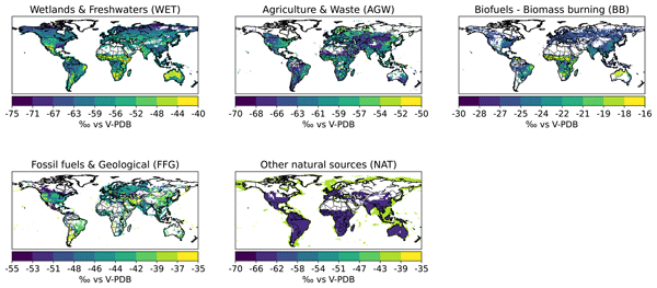
Figure 2 presents the aggregated global maps of δ¹³C-CH₄ source signatures averaged over the period 1998–2022. The spatial variability in these maps reflects both the diversity of isotopic signatures across sub-sectors (see Sect. 1) and the spatial distribution of methane fluxes within each grid cell. The fluxes used for aggregation are detailed in Table 1, which also reports the mean, minimum, and maximum δ¹³C-CH₄ source signatures. Additional maps showing individual sub-sectors are provided in Fig. S1 in the Supplement. The key spatial features for δ¹³C-CH₄ of each sector are summarized below:

• FFG. More enriched signatures (close to −40 ‰) are observed in regions with oil and gas exploitation (e.g. Middle East, USA), while more depleted values (below −50 ‰) occur in coal-dominated, oil sands, or geological seepage areas (e.g. Canada). These patterns reflect the isotopic diversity of fossil sub-sources, as documented in previous studies (Figs. S1 and S2 in the Supplement; Schwietzke et al., 2016; Sherwood et al., 2017; Milkov et al., 2020b; Menoud et al., 2022).

• AGW. Spatial variability results from the balance between depleted livestock emissions ($\sim -\mathrm{66}$ ‰) and more enriched waste-related sources (−51 to −56 ‰). Urbanized regions (e.g. South-East Asia, Europe) show enriched signatures due to dominant landfill and wastewater emissions, whereas rural areas with rice and livestock (e.g. Argentina, Sub-Saharan Africa) are more depleted (Figs. S1 and S2). Livestock signatures show notable regional variability: tropical regions tend to be more enriched (heavier than −60 ‰) due to C₄-dominated forage, while temperate extensive grazing systems on C₃ grasslands yield more depleted values. However, intensive dairy systems in the Northern Hemisphere, fed largely on C₄ maize silage, can also produce relatively enriched signatures (Chang et al., 2019).

• BB. Isotopic gradients are primarily latitudinal, driven by the distribution of C₃ and C₄ plants. Tropical and subtropical regions dominated by C₄ vegetation exhibit more enriched values, while boreal regions show more depleted signatures (Still et al., 2003; Randerson et al., 2012; Lan et al., 2021a). Within the tropics, grass fires burning C₄ vegetation tend to produce more enriched δ¹³C-CH₄ than bush and tree fires, which involve predominantly C₃ biomass (Barker et al., 2020; France et al., 2022).

• WET. Generally depleted values (−50 to −70 ‰) are observed, with more depleted signatures in high-latitude and boreal wetlands, and relatively enriched ones in tropical wetlands, where C₄ aquatic vegetation such as papyrus contribute to isotopically heavier signatures (Ganesan et al., 2018; Oh et al., 2022; Nisbet et al., 2021; France et al., 2022).

• NAT. This sector includes geographically distinct emissions from oceans (more enriched, $\sim -\mathrm{42}$ ‰) and termites (more depleted, $\sim -\mathrm{65}$ ‰). The corresponding isotopic signatures reflect the spatial distribution of each sub-source, as shown in the sub-sector maps (Figs. S1 and S2).

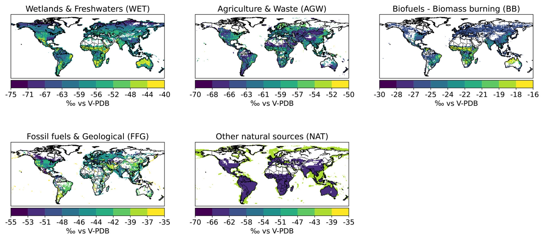
Figure 2 Maps of δ¹³C-CH₄ source signatures (‰) for each of the five source sectors, flux-weighted averages over 1998–2022. Only grid cells with CH₄ fluxes exceeding 0.025 $\mathrm{mg}{\mathrm{CH}}_{\mathrm{4}}{\mathrm{m}}^{-\mathrm{2}}{\mathrm{d}}^{-\mathrm{1}}$ are shown. Note that color scales differ between panels to better highlight spatial patterns within each source sector.

The spatial patterns described above directly influence the simulated atmospheric δ¹³C-CH₄ signal, which may affect the results of inverse modeling. Furthermore, uncertainties in sub-sector isotopic values and their spatial allocation propagate into regional and global inversions, ultimately influencing source attribution. A detailed quantification of these uncertainties is therefore essential to assess their potential impact and guide the design of robust inversion frameworks (Sect. 4.1.3).

The maps also highlight regions where different source types co-occur, potentially complicating the separation of natural and anthropogenic emissions. For example, tropical regions such as Southeast Asia, parts of Africa, and northern South America host both WET and AGW emissions in close proximity. The spatial co-location and similarity of isotopic signatures between these sources can produce blended atmospheric signals, making it challenging to disentangle their respective contributions in top-down inversions. These overlaps underscore the importance of high-resolution spatial and temporal information in both methane fluxes and isotopic signatures to improve source attribution in complex emission environments.

In summary, the updated maps reveal three robust spatial features: a strong north–south gradient in BB and WET signatures driven by ${\mathrm{C}}_{\mathrm{3}}/{\mathrm{C}}_{\mathrm{4}}$ vegetation distribution, a contrast between depleted livestock and enriched waste signatures within AGW, and a marked enrichment over major oil and gas basins for FFG. Regions of source overlap, particularly in the tropics, emerge as priority zones where high-resolution isotopic information is most needed for source attribution.

4.1.2 δ¹³C-CH₄ source signature timeseries

Figure 3 presents the monthly δ¹³C-CH₄ source signature time series for the methane sectors considered in this study over the period 1998–2022. The time series are based on flux-weighted averages. In the following, we describe the temporal evolution and variability of each sector's isotopic signature and discuss the underlying drivers. Most aggregated source sectors show limited temporal variability in their δ¹³C-CH₄ signature over the 1998–2022 period, with typical long-term changes below 1 ‰. The isotopic signature of FFG sources exhibits a slight enrichment over time, increasing from approximately −44.6 ‰ in the early 2000s to around −43.9 ‰ after 2020. Several factors can explain this increase. First, the rapid expansion of shale gas production, particularly in North America after 2010, introduced additional emissions with relatively enriched isotopic signatures compared to conventional natural gas (Milkov et al., 2020a). In the US, shale gas accounted for 48 % of total dry natural gas production in 2013 and reached 82 % by 2023 (IEA, 2013–2023; Saunois et al., 2025). Second, the relative contributions of fossil fuel subsectors have evolved over the past two decades. According to Saunois et al. (2025), based on the synthesis of multiple emission inventories, including EDGARv6.0 and v7.0 (Ferrario et al., 2021; Crippa et al., 2023), GAINSv4.0 (Höglund-Isaksson et al., 2020), CEDS (O'Rourke et al., 2021), the share of coal-related emissions, typically more depleted in δ¹³C-CH₄, increased from approximately 21 % of total fossil fuel emissions in the early 2000s to about 25 % in the 2010s. Meanwhile, oil and gas emissions, associated with less depleted signatures, also grew but were partially counterbalanced by this increasing coal contribution. This sectoral shift has likely moderated the enrichment of the global signature driven by shale gas. Third, geological sources are considered stable over time, both in terms of flux and isotopic signature, providing a background that buffers the sector's temporal variability. Overall, these combined effects explain the modest but persistent enrichment observed in the FFG sector's isotopic signature over the past two decades. No significant seasonal variation is detected for FFG sector, which is consistent with the absence of seasonal modulation in the underlying inventories. However, real-world temporal variability may not be fully captured by inventories. Geopolitical events (e.g. changes in gas trade flows) and evolving gas processing or distribution practices could alter the isotopic composition of emissions over time. While isotopic signatures are generally stable (Schoell et al., 1993), shifts in the relative contribution of end-member sources or changes in gas composition could induce detectable trends (Schwietzke et al., 2014; Sherwood et al., 2017). Such factors remain difficult to assess without dedicated observational constraints.

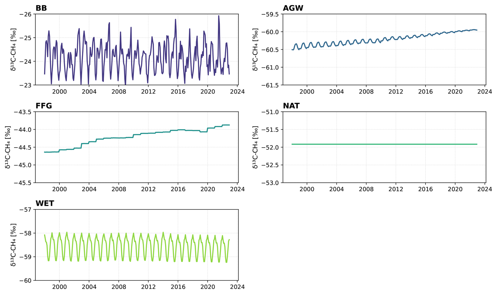
Figure 3 Monthly δ¹³C-CH₄ source signatures from major sectors over the period 1998–2022. Each subplot corresponds to a specific sector (AGW, WET, BB, FFG, NAT).

The AGW signature shows a slight enrichment from about −60.4 to −59.9 ‰. Since the isotopic values of the subcategories (e.g. livestock, wastewater, landfill, rice, and agricultural waste) are held constant, this change reflects a redistribution of fluxes within the AGW sector. Specifically, the relative contribution of livestock and rice cultivation, which together accounted for approximately 69 % of AGW emissions in 2000–2009, decreased to around 68 % in 2010–2019. At the same time, waste-related sources (i.e. landfills, wastewater, and agricultural waste) increased from about 31 % to 32 % of AGW emissions over the same period. This subtle but consistent shift towards more enriched waste sources likely drives the observed isotopic enrichment, particularly in rapidly developing regions with strong urban waste emissions (Saunois et al., 2025). Moreover, the AGW sector exhibits a seasonal cycle in its isotopic signature, primarily driven by rice cultivation, which is the only sub-sector with pronounced seasonal variability in emissions. The slight reduction in the relative contribution of rice, from about 19 % to 16 % of total AGW emissions between 1998–2022, leads to a corresponding decrease in the seasonal amplitude of the δ¹³C-CH₄ signature, reflecting the reduced influence of this highly seasonal sub-sector compared to other more temporally stable AGW sources. In addition to changes in source distribution, long-term shifts in agricultural practices may slightly influence isotopic source signatures. For instance, changes in livestock diet, such as a varying balance between C₃ and C₄ feeds, and large-scale changes in atmospheric δ¹³C-CO₂ may both affect CH₄ isotopic composition. Chang et al. (2019) showed that the progressive depletion of atmospheric δ¹³C-CO₂ since the 1960s, driven by fossil fuel combustion, has led to a corresponding decline in δ¹³C of both C₃ and C₄ plants. This trend propagates through the food chain, ultimately affecting the δ¹³C-CH₄ signature from ruminants. Although such effects likely occur, they are not yet explicitly represented in our dataset due to a lack of systematic isotopic observations that track temporal changes in agricultural feedstocks or cultivation practices.

The WET isotopic signature remains largely stable over the period 1998–2022, with only a minor change from approximately −58.6 to −58.7 ‰, consistent with the trend reported by Oh et al. (2022). More importantly, wetlands exhibit a strong seasonal cycle in δ¹³C-CH₄ signatures, with more depleted values during the summer months. This seasonal variation is driven by the dominance of methane emissions from boreal wetlands during summer, which are isotopically lighter than emissions from tropical wetlands (Oh et al., 2022).

The BB isotopic signature remains stable around −24.3 ‰ throughout the study period, consistent with the identical δ¹³C-CH₄ signatures prescribed for biomass burning and biofuel burning subcategories (Lan et al., 2021a). However, the sector exhibits a pronounced seasonal cycle, with less depleted values during the boreal winter. This pattern reflects the higher contribution of biomass burning emissions from the Southern Hemisphere during this period, which are characterized by relatively enriched δ¹³C-CH₄ signatures (see Fig. 2).

The NAT isotopic signature remains constant throughout the period, as expected. Values for both subcategories (oceanic and termites) are derived using climatological fluxes and fixed δ¹³C-CH₄ values, leading to negligible variability over time.

In summary, four sectors (FFG, AGW, BB, WET) show modest but identifiable temporal signals over 1998–2022: a slight FFG enrichment driven by shale gas expansion partially offset by rising coal contributions, a slight AGW enrichment from increasing waste shares, a stable BB mean with strong seasonal cycles, and a stable WET mean with strong boreal-summer-driven seasonality. NAT remains constant by construction. These temporal patterns are small (typically <1 ‰) but systematic, and should be preserved in inversion priors.

4.1.3 Uncertainty in δ¹³C-CH₄ source signature

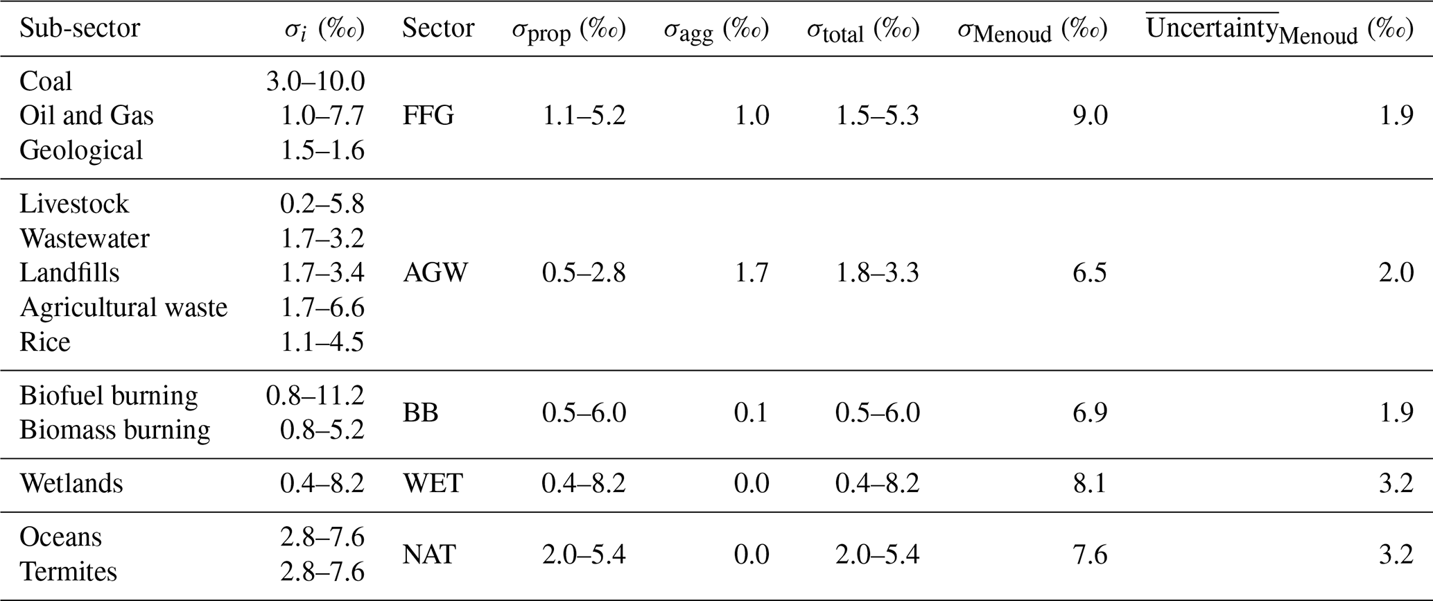
Table 4 presents the uncertainty ranges associated with the δ¹³C-CH₄ source signatures for each major sector and their respective sub-sectors. The uncertainty in aggregated δ¹³C-CH₄ source signatures arises from two primary components: (1) the variability across sub-sectors, expressed first as the range of sub-sector uncertainties (σ_i), and then as a flux-weighted propagated uncertainty to the sector level (σ_prop), and (2) the aggregation uncertainty (σ_agg), reflecting the sensitivity of sectoral signatures to the prior flux distribution used for aggregation (see methodology in Sect. 2.3). In the following, we first analyse the uncertainty intrinsic to each sectors, then examine the additional uncertainty introduced by aggregation at the sector level, and finally discuss the total propagated uncertainties and their implications for methane source attribution.

Table 4 Summary of uncertainty estimates for aggregated δ¹³C-CH₄ source signatures by sector (in  ‰), based on data from 2016–2020. Sector acronyms are as follows: FFG = Fossil Fuels and Geological sources, AGW = Agriculture and Waste, BB = Biomass and Biofuel Burning, WET = Wetlands, NAT = Other Natural sources. σ_i refers to the range of isotopic uncertainties across sub-sectors (in  ‰). These are taken from Lan et al. (2021a) (lower bound) and Menoud et al. (2022) (upper bound). The sub-sector uncertainty for geological sources is taken from Etiope et al. (2019). σ_prop represents the sector-level propagated uncertainty, derived from the flux-weighted combination of sub-sector uncertainties. σ_agg corresponds to the uncertainty introduced by the aggregation method, based on sensitivity tests using different prior flux inventories. σ_total is the total combined uncertainty, calculated as ${\mathit{\sigma }}_{\text{total}}=\sqrt{{\mathit{\sigma }}_{\text{prop}}^{\mathrm{2}}+{\mathit{\sigma }}_{\text{agg}}^{\mathrm{2}}}$. σ_Menoud and ${\stackrel{\mathrm{‾}}{\text{Uncertainty}}}_{\text{Menoud}}$ refer to the standard deviation and mean uncertainty reported by Menoud (2022) across all available literature. Note that since σ_prop is derived from the same base dataset, the propagated and total uncertainties (σ_prop, σ_total) are not fully independent of σ_Menoud and ${\stackrel{\mathrm{‾}}{\text{Uncertainty}}}_{\text{Menoud}}$, but provide complementary comparison insight.

Propagated uncertainty from sub-sectors (σ_prop)

The propagated uncertainty at the aggregated sector level, denoted σ_prop, captures the combined effect of isotopic variability among sub-sectors within each source category. It is computed using a flux-weighted combination of individual sub-sector uncertainties (σ_i), as described in Sect. 2.3. These sub-sector uncertainties reflect both the intrinsic heterogeneity of emission processes and the spread of values reported in the literature. The resulting σ_i and σ_prop values for each sector are summarized in Table 4. Below, we describe the dominant contributors to σ_prop, ordered from highest to lowest sectoral uncertainty.

• WET exhibits the largest propagated uncertainty (σ_prop=0.4–8.2 ‰), directly inherited from the wide range of sub-sector values (σ_i=0.4 ‰–8.2 ‰). The high variability reflects the influence of multiple environmental factors, including substrate type, methanogenic pathways (acetate fermentation vs. CO₂ reduction), and the δ¹³C content of the organic matter (Ganesan et al., 2018; Oh et al., 2022). Tropical wetlands in particular remain under-sampled, despite representing a dominant fraction of global wetland CH₄ emissions (France et al., 2021, 2022).

• BB displays a propagated uncertainty of 0.5–6.0 ‰. This stems from the isotopic contrast between C₃ and C₄ vegetation: C₄ plants tend to produce more enriched δ¹³C-CH₄ during combustion. The range of σ_i (0.8–11.2 ‰) reflects differences in vegetation type across ecosystems and latitudes (Chanton et al., 2000; Brownlow et al., 2017; Menoud et al., 2022), with tropical fire-dominated regions being particularly under-represented in isotopic measurement databases (Nisbet et al., 2021).

• NAT show a high sectoral uncertainty (σ_prop=2.0 ‰–5.4 ‰), driven by the strong isotopic contrast for oceanic and termite sub-sectors. Both sub-sectors exhibit broad σ_i values (2.8–7.6 ‰), reflecting limited measurement coverage and substantial environmental dependency.

• FFG sources encompass oil, gas, coal, and geological seepage, each with distinct isotopic characteristics. The coal sub-sector, in particular, contributes significantly to the sector-level propagated uncertainty (σ_prop=1.1 ‰–5.2 ‰) due to its high variability (σ_i=3.0 ‰–10.0 ‰). The diversity in extraction technologies (e.g. conventional vs. unconventional gas), geological formations (e.g. shale vs. coalbed), temporal shift and regional practices leads to strong heterogeneity and uncertainty in fossil fuel signatures (Lan et al., 2021a; Menoud et al., 2022).

• AGW exhibits the lowest sectoral propagated uncertainty among the sectors (σ_prop=0.5 ‰–2.8 ‰), despite moderate to high sub-sector variability (σ_i=0.2 ‰–6.6 ‰). This is due to a flux-weighted balancing effect between well-characterized sources.

Beyond sectoral aggregation, the propagated uncertainties also exhibit a latitudinal structure. The distribution of C₃ and C₄ plants drives systematic gradients in isotopic signatures across the WET, BB, and AGW sectors: tropical regions, dominated by C₄ vegetation, tend to produce more enriched δ¹³C-CH₄ signatures, while boreal and temperate regions, where C₃ plants prevail, yield more depleted values (Still et al., 2003; Chang et al., 2019; France et al., 2022; Nisbet et al., 2021). This latitudinal gradient contributes a spatially structured component to isotopic uncertainty that is not fully captured by global or regional averages.

These propagated uncertainties from sub-sectors highlight the need for more systematic and representative measurements, particularly in under-sampled regions (e.g. tropics), and sectors (e.g. coal mines). The scarcity of isotopic measurements in tropical regions is a critical limitation: despite hosting some of the largest CH₄ sources globally, including tropical wetlands, rice paddies, and livestock systems, these regions remain under-represented in isotopic databases (Nisbet et al., 2021; France et al., 2022). Targeted field campaigns and isotopic monitoring networks could help reduce this uncertainty. Nonetheless, because of the inherent diversity and variability of methane formation processes, some degree of irreducible uncertainty must be accounted for and formally propagated in inversion frameworks (see Sect. 4.3.2).

Aggregation uncertainty (σ_agg)

Aggregation is primarily required for computational efficiency in inversion frameworks (Sect. 2.2). But, this necessary simplification introduces methodological uncertainty that must be explicitly quantified and propagated (Sect. 2.3). The aggregation uncertainty, denoted σ_agg, represents the error introduced when multiple sub-sectors are combined into a single aggregated sector based on their respective emission fluxes. The corresponding values for each sector are reported in Table 4. Although this component is generally smaller and more stable than σ_prop, it increases for sectors that involve several formation pathways and isotopic fractionation, such as FFG (1.0 ‰) and AGW (1.7 ‰), where heterogeneous sub-sector compositions lead to significant propagation effects. These values illustrate that choices made in emission inventories, not only in flux magnitudes but also in source definitions and partitioning, can significantly shape sector-level isotopic signatures.

Notably, discrepancies among major methane inventories, including EDGARv8 (Crippa et al., 2023), GAINSv4 (Höglund-Isaksson et al., 2020), CEDSv2021 (O'Rourke et al., 2021), and GFEIv2 (Scarpelli et al., 2022), contribute significantly to this aggregation uncertainty. For instance, for the FFG sector, the aggregation uncertainty is around 2.2 % at the global scale, reflecting heterogeneity across inventories. Variability in emission factors and inventory methodologies, as described in Saunois et al. (2025), contribute strongly to this uncertainty. For example, oil and gas system emissions estimates vary considerably due to differences in emission factors and methodological assumptions across countries and inventories. Similarly, for the AGW sector, the aggregation uncertainty (2.8 %) reflects differences in how fluxes are allocated among agriculture and waste-related sub-sectors across inventories. For example, manure emissions can be allocated either to the agriculture or to the waste category, which can shift the aggregated isotopic signature. On the contrary, for WET, no aggregation uncertainty is reported because this sector relies on a single wetland flux dataset for weighting, precluding a cross-inventory sensitivity assessment. We note, however, that the latitudinal contrast between tropical (more enriched, $\sim -\mathrm{50}$ ‰) and boreal (more depleted, $\sim -\mathrm{70}$ ‰) wetlands contributes substantially to the propagated uncertainty σ_prop already reported for this sector (0.4 ‰–8.2 ‰). For NAT, since termite and ocean sources do not overlap geographically, the aggregation uncertainty is null.

Total uncertainty (σ_total)

The total uncertainty, σ_total, represents the combined effect of sub-sector variability and aggregation uncertainty. The full range of uncertainty values per sector (σ_total) is reported in Table 4. This range corresponds to the spread of possible standard deviations (i.e. the uncertainty spread) rather than to a range of actual δ¹³C-CH₄ signature values. This total uncertainty varies across sectors. For example, the BB and WET sectors exhibit wide uncertainty ranges, from 0.5 ‰ to 6.0 ‰ and from 0.4 ‰ to 8.2 ‰, respectively, primarily driven by sub-sector uncertainties. For the BB sector, the total uncertainty is largely driven by the sub-sector variability of biofuel burning. For WET, the large uncertainty is mainly due to the inherent spatial and seasonal variability of wetland emissions. The FFG and AGW sectors show total uncertainties of up to 5.3 ‰ and 3.3 ‰, respectively, which is consistent with their source diversity and complex sub-sector structures. NAT sources display lower average uncertainties overall.

The columns σ_Menoud (standard deviation within the dataset) and ${\stackrel{\mathrm{‾}}{\text{Uncertainty}}}_{\text{Menoud}}$ (mean uncertainty) in Table 4 offer a comparison with extensive literature compilations (Menoud, 2022). Our total uncertainties are comparable to or smaller than these literature-based estimates, suggesting that the applied aggregation methodology provides a structured and quantitative framework for uncertainty propagation that complements broader bibliographic syntheses. However, the sub-sector uncertainties (σ_prop) used in our calculations are derived from the same dataset compiled by Menoud (2022). Therefore, σ_prop and σ_total are not fully independent from the comparison values in σ_Menoud and ${\stackrel{\mathrm{‾}}{\text{Uncertainty}}}_{\text{Menoud}}$. The comparison is nonetheless informative as it illustrates how the literature-based source variability propagates through our aggregation scheme.

These sectoral uncertainties are subsequently propagated in our sensitivity simulations (see Sect. 3.2). They serve as a quantitative basis for defining the plausible variability ranges of source signatures, allowing us to assess their influence on modeled atmospheric δ¹³C-CH₄ distributions. A complementary qualitative assessment of systematic biases inherited from the underlying observational databases (e.g. uneven geographic coverage, methodological heterogeneity, limited temporal representativeness) is provided in Sect. 4.1.4. In atmospheric inversion frameworks, the total sectoral uncertainty (σ_total) can also be used to inform the specification of the prior error covariance matrix (B matrix) (see Sect. 4.3.2).

Overall, the sectors rank by total uncertainty as WET (0.4 ‰–8.2 ‰) > BB (0.5 ‰–6.0 ‰) > NAT (2.0 ‰–5.4 ‰) > FFG (1.5 ‰–5.3 ‰) > AGW (1.8 ‰–3.3 ‰). Sub-sector variability dominates over aggregation effects in all sectors, and the largest reducible uncertainties lie in tropical wetlands and biomass burning regions where measurements remain sparse. These sectoral uncertainties are directly used in the sensitivity simulations (Sect. 3.2) and inform B matrix specification in inversion frameworks (Sect. 4.3.2).

4.1.4 Comparison with δ¹³C-CH₄ datasets from previous studies

For the FFG sector, our weighted mean signature is −44.2 ‰, which is generally consistent with Lan et al. (2021a) but slightly more enriched compared to Menoud et al. (2022) and Thanwerdas et al. (2024) whose values extend to more depleted ranges. Coal sources show greater differences, with our estimate around −43.7 ‰ compared to −50.7 ‰ in Menoud et al. (2022). This discrepancy can be explained by differences in data selection criteria and spatial weighting. Our estimate is derived using flux-weighted averaging that emphasizes high-emitting coal regions, such as China and India, where emissions tend to be less depleted than the global average (e.g. Wei et al., 2014; Qin et al., 2006; Sherwood et al., 2017; Lan et al., 2021a). In contrast, the value reported by Menoud et al. (2022) is an arithmetic mean of a broad compilation of site-level measurements, including more depleted coal emissions from regions with lower production or different geological contexts. The oil and gas isotopic signature is close to previous studies, with minor variation likely due to regional refinements. Geological emissions are fixed at −46.6 ‰, in line with the geochemical value from Etiope et al. (2019).

In the AGW sector, livestock methane isotopic values (−65.8 ‰) are more depleted than reported by Menoud et al. (2022) (−63.0 ‰) and Thanwerdas et al. (2024) (−63.6 ‰). This difference likely stems from our use of the spatially explicit source signature maps from Lan et al. (2021a), which account for regional differences in ${\mathrm{C}}_{\mathrm{3}}/{\mathrm{C}}_{\mathrm{4}}$ feed composition using global maps of biomass ${\mathrm{C}}_{\mathrm{3}}/{\mathrm{C}}_{\mathrm{4}}$ ratios (Randerson et al., 2012; Still et al., 2003). Flux-weighted averaging based on these maps emphasizes regions dominated by C₃ vegetation, such as temperate zones, resulting in more depleted signatures. Our estimate is also consistent with the −64.9 ‰ value reported for 2012 by Chang et al. (2019). Waste-related emissions, including landfill, wastewater, and agricultural waste, are updated following Menoud et al. (2022), resulting in relatively values: −50.9 ‰ for wastewater, −56.2 ‰ for landfill, and −54.9 ‰ for agricultural waste. Our landfill and wastewater values align with Menoud et al. (2022) but differ by 2 ‰–4 ‰ from Lan et al. (2021a) and Thanwerdas et al. (2024). This increase is attributed to changes in waste management practices, notably increased biogas production, which tends to leak methane with relatively higher δ¹³C (Menoud et al., 2022). For agricultural waste specifically, the inter-dataset spread (−52 to −57.8 ‰) exceeds the sub-sector uncertainty σ_i, pointing to genuine methodological heterogeneity in the definition of this sub-sector (crop residues vs. manure vs. composting). Rice emissions, also from Menoud et al. (2022), are set at −59.9 ‰, slightly more enriched than the −63.0 ‰ used in Thanwerdas et al. (2024) due to differences in the amount of compiled literature.

For BB, our weighted mean of −24.3 ‰ from Lan et al. (2021a) matches closely the value from Thanwerdas et al. (2024), while being slightly more depleted than in Menoud et al. (2022). WET signatures, derived largely from Oh et al. (2022), have a weighted mean of −58.6 ‰, slightly enriched compared to Menoud et al. (2022) (−63.3 ‰) and consistent with Lan et al. (2021a). The ∼4.7 ‰ offset with Menoud et al. (2022) reflects the over-representation of boreal measurements in their literature compilation vs. our flux-weighted average, which emphasizes tropical wetlands. Recent tropical airborne measurement programs report wetland source signatures of $-\mathrm{59.0}\pm \mathrm{1.3}$ ‰ in Bolivian Amazonia (France et al., 2022) and $-\mathrm{59.3}\pm \mathrm{2.0}$ ‰ for a Zambia–Bolivia composite (Nisbet et al., 2021), consistent with the tropical wetland values used in our maps from Oh et al. (2022). The slightly more enriched values produced by our maps over African papyrus-dominated wetlands likely reflect that these recent airborne measurements have not yet been assimilated into process-based wetland isotope models, contributing to the systematic biases on tropical wetlands discussed below.

Natural sources (NAT) retain previous estimates, with termites at −63.4 ‰ and oceans at −42.0 ‰, reflecting values from Lan et al. (2021a) and Thanwerdas et al. (2024). The weighted mean of −51.9 ‰ accounts for the relative contribution of these sources. For termites, we adopted a value of −63.4 ‰, consistent with Lan et al. (2021a) and Thanwerdas et al. (2024). The depleted signature of −76.1 ‰ reported by Sugimoto et al. (1998) was not used here due to concerns about potential outliers. This choice explains the discrepancy with the more depleted mean of Menoud et al. (2022), who included the Sugimoto et al. (1998) value in their compilation.

Beyond these sub-sector-specific differences, the inter-dataset inconsistencies are of the same order as the sub-sector uncertainty σ_i and point to systematic biases inherited from the underlying observational databases, which σ_i does not capture. At the sub-sector level, σ_i reflects the statistical dispersion within the sampled measurements (Menoud et al., 2022), not the representativeness of that sample relative to the true global distribution of emission sources. We identify three main systematic biases:

• Uneven geographic coverage: the compilation from Sherwood et al. (2017, 2021) underlying Lan et al. (2021a) is dominated by North American data, EMID (Menoud et al., 2024) improves European coverage but Africa, South America, and large parts of Asia remain under-sampled; tropical wetlands are represented through fewer campaigns than boreal/temperate ones, and recent tropical measurement programs (France et al., 2022; Nisbet et al., 2021; Shaw et al., 2022) have not yet been integrated;

• Methodological heterogeneity: literature signatures are arithmetic means while our sector values are flux-weighted;

• Limited temporal representativeness: signatures are held constant for most sub-sectors over 1998–2022, while documented trends linked to evolving livestock feed composition or gas processing practices (Chang et al., 2019) are not explicitly represented.

The propagation of these biases to the aggregated maps depends on the flux-weighting scheme: biases affecting small-flux sub-sectors (termites, oceans) have limited impact, while those affecting high-emitting sub-sectors (livestock, oil and gas, tropical wetlands) propagate more directly to the modeled atmospheric δ¹³C-CH₄ signal, consistent with the sensitivity hierarchy reported in Table 6.

Menoud et al. (2022)Lan et al. (2021a)Thanwerdas et al. (2024)

Table 5 Globally averaged δ¹³C-CH₄ values (‰) for each source sector, weighted by methane flux over 1998–2022. Flux-weighted mean values were calculated using a consistent methane flux dataset across sectors and years (see Table 1), but only in cases where δ¹³C-CH₄ signatures vary spatially or when aggregating sub-sectors. For literature datasets (e.g. Menoud et al., 2022; spatially fixed values for Lan et al., 2021a and Thanwerdas et al., 2024), the reported values correspond to simple arithmetic means and are not flux-weighted. Ranges in brackets indicate minimum and maximum of mean value over time. Numbers in parentheses denote the number of measurements used in the respective studies. Bold font indicates the flux-weighted “Weighted mean” rows (aggregated sector values).

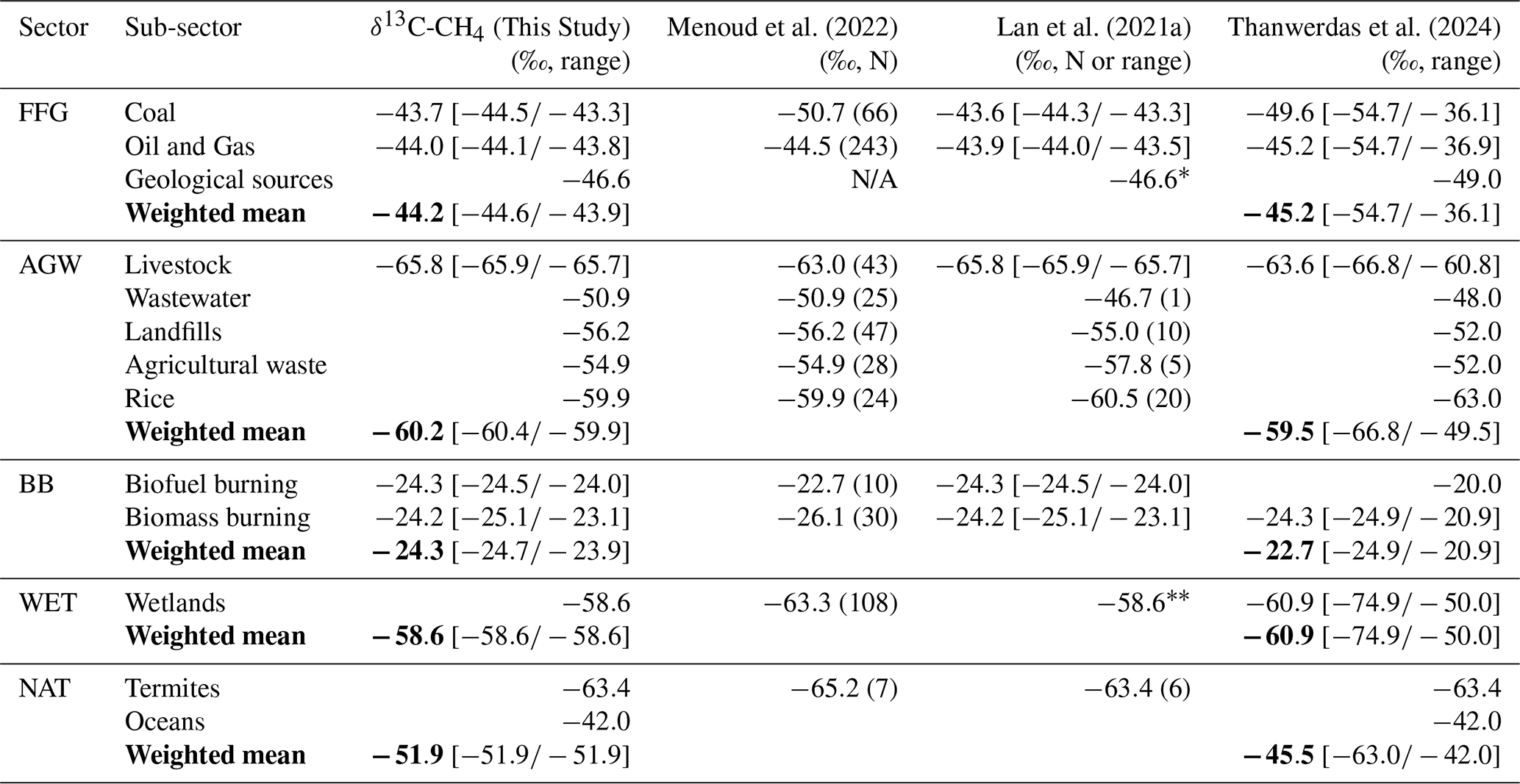
^* Value from Etiope et al. (2019). ${}^{**}$ Value from Oh et al. (2022).

Table 6 Summary of the sensitivity of modeled CH₄ mole fraction and δ¹³C-CH₄ signal to key parameters at surface level over 2016–2020. Values are given as relative and absolute standard deviations (first and second number in each cell, respectively). Note that the Cl sink is not perturbed independently in this sensitivity ensemble. This impact within the same CIF–LMDz–SACS framework has been comprehensively quantified by Thanwerdas et al. (2022b), who report that stratospheric Cl alone contributes a ∼0.30 ‰ surface enrichment in δ¹³C-CH₄ via stratosphere–troposphere exchange, and modifies the seasonal cycle amplitude by 10 %–20 % depending on latitude, see Sect. 4.2.3 for further discussion.

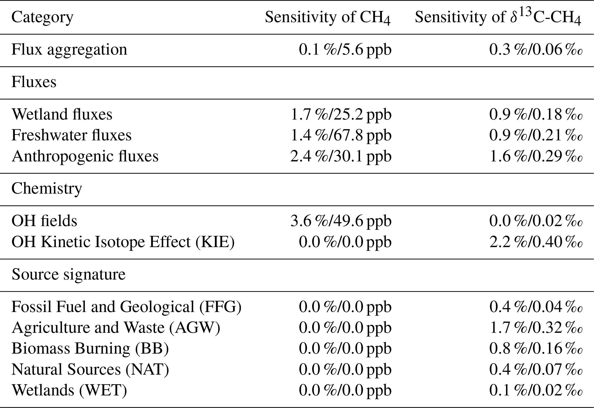
Generally, the updated δ¹³C-CH₄ source signature maps show clear sectoral and regional patterns, with depleted signatures for wetlands and agriculture, and enriched signatures for fossil fuel and biomass burning emissions. Temporal variations are limited over the study period, except in sectors where emissions were known to vary in time. Uncertainty analysis highlights significant variability, particularly for the agriculture and waste sector. The updated maps are broadly consistent with recent datasets. In the next section, we assess how the uncertainties over inputs propagate to the modeled atmospheric δ¹³C-CH₄ signal through sensitivity simulations.

4.2 Sensitivity of simulated atmospheric δ¹³C-CH₄ signal and CH₄ mole fractions to key parameters

Forward atmospheric simulations provide a framework for assessing the impact of source signature uncertainties on modeled δ¹³C-CH₄ (see Sect. 3.1). By testing several sets of key input parameters (see Sect. 3.2), we can identify which sources of uncertainty have the strongest influence on the atmospheric isotopic signal. This approach, and the way input and output uncertainties are propagated within the inversion framework, is illustrated in Fig. 4. In this section, we evaluate the sensitivity of simulated atmospheric CH₄ mole fractions and δ¹³C-CH₄ isotopic signals at the surface, where observations are available, to key parameters, including emission inventories for aggregation (Sect. 4.2.1), fluxes (Sect. 4.2.2), chemical reactions (Sect. 4.2.3), and source signatures (Sect. 4.2.4). Table 6 provides a comparative overview of the sensitivities, allowing a quick identification of which parameters most influence the modeled CH₄ mole fractions and isotopic signals. Detailed results and interpretations are provided in the following sub-sections.

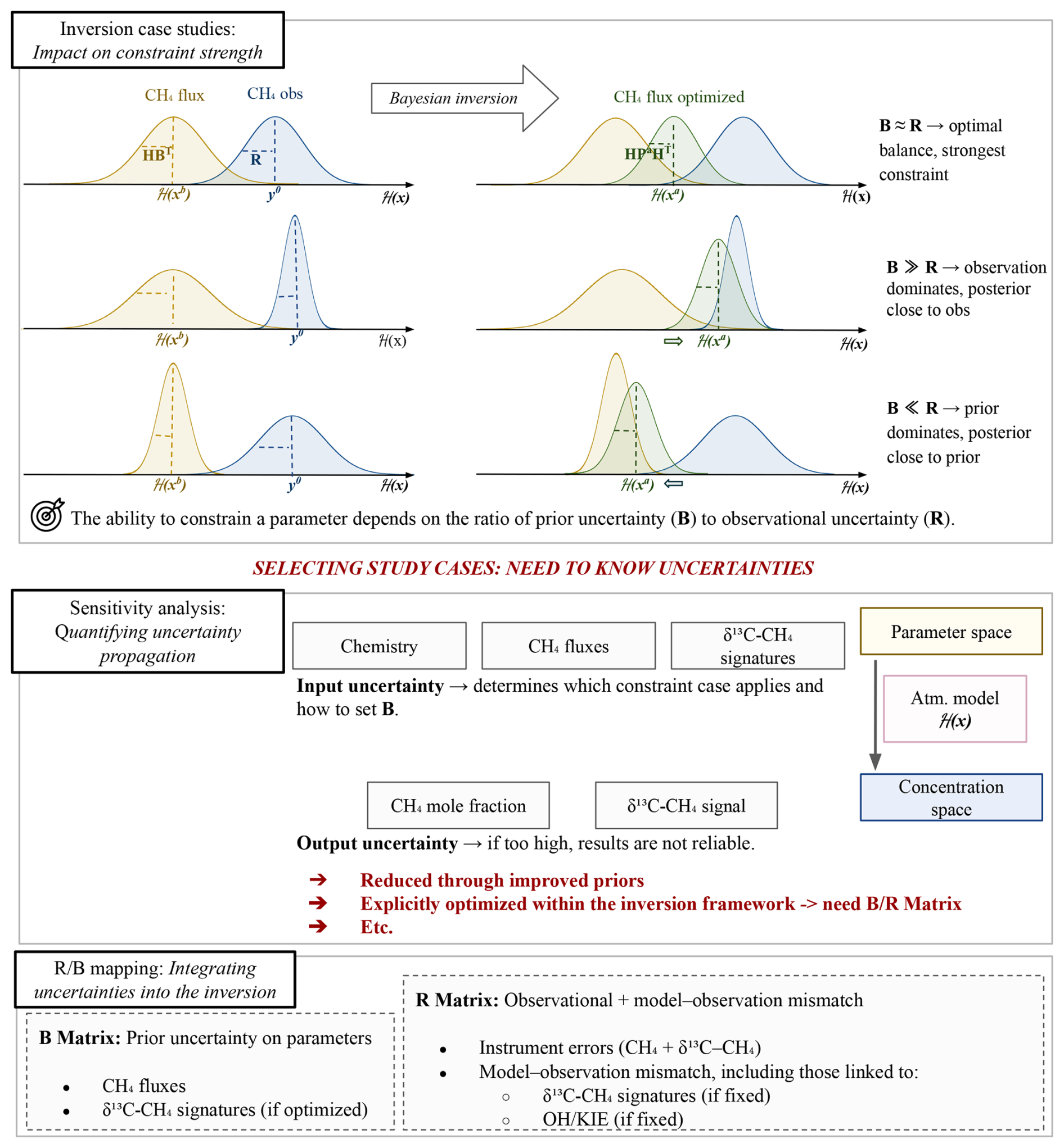
Figure 4 In the upper panel, coloured Gaussian curves (yellow: prior, blue: observation, green: posterior) illustrate how the ratio between B (prior error covariance matrix) and R (observation error covariance matrix) determines the strength of the inversion constraint: (i) when B≈R, the optimal balance yields the strongest constraint; (ii) when B≫R, observations dominate and the posterior approaches the observations; (iii) when B≪R, the prior dominates and the posterior remains close to the prior. The middle panel conceptually shows how uncertainties are quantified in the sensitivity framework. Input uncertainties determine which constraint case applies and how to set B in the parameter space, which is mapped into the concentration space by the atmospheric model operator ℋ(x). Output uncertainties indicate the reliability of the inversion results; if too high, results are not robust. They can be reduced through improved priors or explicitly optimized within the inversion framework. The bottom panel summarises how these uncertainties are formalised within the B matrix and the R matrix.

4.2.1 Sensitivity to fluxes used for aggregation

We note that the term “aggregation” is used in two distinct methodological senses in this section. The first refers to the choice of flux inventory used to weight sub-sector isotopic signatures into sector-level values, which generates the aggregation uncertainty σ_agg reported in Table 4 (AGGREG_EDGAR, AGGREG_GFEI, AGGREG_CEDS and AGGREG_GAINS simulations). The second refers to the sectoral granularity of the atmospheric model itself, i.e. the number of source categories effectively transported (5 by default vs. 14 in the NO_AGGREG simulation). Both are tested below but answer complementary questions: the former probes the sensitivity of the aggregated signature values, while the latter probes the sensitivity of the modeled atmospheric signal to the level of sub-sector resolution.

Figure 5 summarizes the sensitivity of flux aggregation to different prior datasets. Panel (a) shows the variability of flux estimates between inventories, highlighting where emission fluxes are most uncertain. Since this test focuses specifically on uncertainties arising from the flux-weighted aggregation of isotopic signatures, only anthropogenic sectors (FFG, AGW and BB) are included (see Sect. 3.2). Panel (b) presents the resulting variability in the aggregated δ¹³C-CH₄ source signatures by sector. Panel (c) shows the sensitivity of simulated atmospheric δ¹³C-CH₄ signals to these aggregated isotopic changes at surface level. It is important to note that panel (c) displays a single sensitivity map representing the combined impact of flux-weighted isotopic signatures variations across all anthropogenic sectors on isotopic signal simulated at the surface. Because only isotopic signatures are perturbed while the underlying emission fluxes remain unchanged, this test does not directly affect CH₄ mole fractions. The only noticeable effect on CH₄ mole fractions occurs in the “NO_AGGREG” setup, in which the number of aggregated source categories was increased from 5 to 14 to evaluate the impact of the trade-offs between computational efficiency and isotopic detail (see Sect. 3.2), resulting in a very small change in simulated CH₄ mole fractions (about 5.6 ppb on average; Table 6). Figure S3 in the Supplement shows the same information as in Fig. 5 but expressed in terms of relative standard deviation (RSD). Together, these results illustrate how inventory discrepancies propagate through to atmospheric simulations of δ¹³C-CH₄ signal.

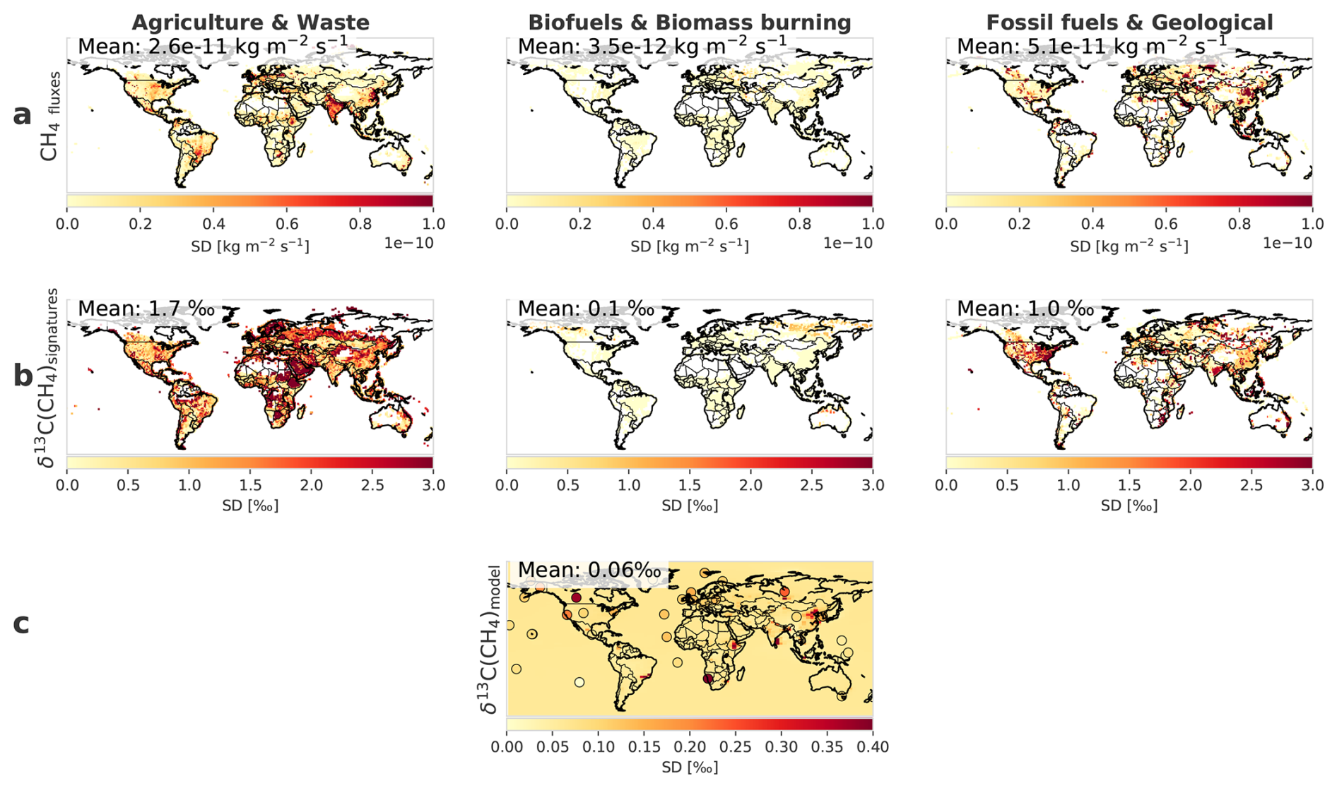
Figure 5 (a) SD (in $\mathrm{kg}{\mathrm{m}}^{-\mathrm{2}}{\mathrm{s}}^{-\mathrm{1}}$) of the fluxes among different prior datasets (GAINSv4, CEDSv2021, GFEIv2, EDGARv8) (over 2016–2020) at surface level. Values are only displayed when the associated CH₄ flux is higher than 0.2 $\mathrm{mg}{\mathrm{CH}}_{\mathrm{4}}{\mathrm{m}}^{-\mathrm{2}}{\mathrm{d}}^{-\mathrm{1}}$, for aggregated categories. (b) SD in ‰ of the δ¹³C-CH₄ source signature by aggregated category at surface level. (c) SD in ‰ of the δ¹³C-CH₄ signals from the forward model outputs at surface level. Coloured circles indicate SD of observed δ¹³C-CH₄ values at each surface station over the study period (Michel et al., 2024; Schuldt et al., 2025).

The largest flux uncertainties (Fig. S3a in the Supplement) are observed in the Fossil Fuels and Geological (FFG) and Agriculture and Waste (AGW) sectors (65 % and 41 % respectively). These uncertainties stem from differences between inventories, which exhibit regional discrepancies. For example, in Central Asia (Turkmenistan, Afghanistan, Uzbekistan), there are significant differences in fossil fuel emission estimates. In Turkmenistan, GAINS estimates 1259 kt CH₄ yr⁻¹, while EDGARv8 and CEDS report 1343 and 1351 kt CH₄ yr⁻¹ respectively and GFEI 888 kt CH₄ yr⁻¹. Although totals appear similar, the spatial allocation and sectoral breakdown differ markedly between inventories. This is partly because inventories rely on national reports submitted to the UNFCCC, ensuring consistency at the country level but not necessarily in spatial detail or sub-sector attribution. Additionally, satellite-based studies (e.g. Vanselow et al., 2024) have identified emission events in regions such as Turkmenistan, associated with fossil fuel infrastructure. However, such episodic or localized emissions are generally not included in bottom-up inventories, which may underestimate the true emission rates. In the AGW sector, a high RSD is observed in Botswana. This is linked to the aggregation structure in GAINS, where large African regions are aggregated, whereas other inventories provide country-level estimates.

The impact of these flux uncertainties on δ¹³C-CH₄ source signatures (Fig. 5b) is especially pronounced in the AGW sector, which shows the highest isotopic sensitivity (1.7 ‰), particularly in the Middle East and parts of Africa. This is related to the relative contributions of sub-sectors with distinct isotopic signatures, such as livestock (more depleted) and waste (less depleted), as defined in the inventories. For instance, in Ethiopia (2016–2020), livestock accounts for 79 % of AGW emissions in CEDS and GAINS, but only 67 % in EDGARv8, which is reflected in the region's isotopic signature variability. Regional variations in livestock diets, driven by the local balance between C₃ and C₄ forage plants, further contribute to this spread (Chang et al., 2019). For instance, in Ethiopia, the balance between C₃ and C₄ forage grasses varies with altitude, leading to distinct isotopic signatures within the same country (Brychkova et al., 2022). AGW is disaggregated in our framework into five sub-sectors (livestock, rice, landfills, wastewater, and agricultural waste; Table 1), each with its own isotopic signature and flux distribution. Livestock and rice together account for ∼62 % of AGW emissions and carry the most depleted signatures (−65.8 ‰ and −59.9 ‰), while waste-related sub-sectors (−50.9 to −56.2 ‰) make up the remaining 38 %. This contrast is the main driver of the propagated uncertainty σ_prop reported for AGW in Table 4. To assess whether finer sectoral granularity, i.e. the number of source categories effectively resolved in the atmospheric model, would meaningfully change the modeled atmospheric signal, the NO_AGGREG simulation increases the number of source categories from 5 to 14 (Table 3). This is conceptually distinct from the aggregation uncertainty σ_agg defined in Sect. 2.3.3, which quantifies the sensitivity of the aggregated signature to the choice of flux inventory used for weighting (Fig. 5). The resulting differences are small: +0.061 ‰ globally for δ¹³C-CH₄ (Fig. S4 in the Supplement). Localized differences of up to ±0.5 ‰ in δ¹³C-CH₄ occur in regions where sub-sector composition contrasts strongly with the global average, notably in South Asia and the Middle East. These results indicate that increasing sectoral granularity beyond five sub-sectors does not substantially alter the modeled atmospheric isotopic signal at the global scale. Reducing AGW-related uncertainty would therefore benefit more from better-constraining the signature values of the existing sub-sectors and from refining inventory-level flux partitioning between livestock and waste, particularly in rapidly developing regions, than from increasing the number of source categories.

In contrast, the FFG sector shows lower isotopic sensitivity despite higher flux uncertainties (2.2 %). This is explained by the more homogeneous isotopic signatures of coal, oil and gas and geological, and the smaller relative isotopic differences among sub-sectors. The uncertainties are highest in North America, they are mainly associated with the difference in relative contribution of oil and gas vs. coal in the datasets. The variability in Chinese coal emissions is also well documented, with CEDS based on EDGARv4.2 previously overestimating emissions compared to recent regional inventories (Liu et al., 2021; Saunois et al., 2025). These results highlight the key role of emission partitioning within aggregated categories in shaping the final isotopic source signature, particularly in the AGW sector. These uncertainty values are used to define the σ_agg parameter in the uncertainty analysis (see Sect. 4.1.3).

The sensitivity of simulated atmospheric δ¹³C-CH₄ signals to aggregation choices remains globally low, with a mean RSD of 0.32 % (Fig. S3c in the Supplement) and a mean SD of approximately 0.06 ‰ (Fig. 5c). This suggests that, despite regional discrepancies, aggregation uncertainties have a limited impact on large-scale atmospheric isotopic patterns. Moreover, the values shown in Fig. S3c represent relative sensitivities computed over the entire model domain, which tends to dilute localized sensitivity hotspots. When compared to the RSD of observed δ¹³C-CH₄ values at surface stations (e.g. Michel et al., 2024; Schuldt et al., 2025), the simulated sensitivities is smaller. This indicates that real-world atmospheric variability exceeds the response induced by inventory-driven aggregation uncertainties, and further support the limited impact of this specific error source on the modelisation of the atmospheric isotopic signal at observational sites (more details in Sect. 4.3).

In summary, two distinct aggregation-related effects have been tested in this section. First, the choice of flux inventory used to weight sub-sector signatures (the aggregation uncertainty σ_agg) introduces sizeable variability in the aggregated signature values themselves, notably for AGW and FFG, but propagates only weakly to the modeled atmospheric δ¹³C-CH₄ signal. Second, increasing the sectoral granularity from 5 to 14 source categories (NO_AGGREG test) modifies the modeled signal by only +0.06 ‰ globally. Both aggregation-related choices therefore have a limited impact on atmospheric simulations, supporting the transferability of the updated maps across inversion systems and inventories.

4.2.2 Sensitivity to uncertainties in methane fluxes from wetlands, freshwaters, and anthropogenic sectors

Figure 6 summarizes the sensitivity of atmospheric simulations to uncertainties in methane flux estimates from key source sectors: wetlands, freshwaters, and the total anthropogenic emissions (i.e. the sum of all anthropogenic sources). Unlike the previous section, where only isotopic signatures were perturbed through flux-weighted aggregation, here the underlying emission fluxes themselves are varied in the model simulations. Panel (a) shows the SD of CH₄ emissions across inventories, and highlight where flux uncertainties are the greatest. For a detailed breakdown of anthropogenic subsectors (e.g. fossil fuels, waste, agriculture), refer to Figs. S6 and S7 in the Supplement, which show their individual contributions. Panels (c) and (e) display the impact of uncertainties in wetlands, freshwaters, and anthropogenic fluxes on modeled CH₄ mole fractions and δ¹³C-CH₄ signals, respectively, at surface level. Figure S5 in the Supplement shows the same information in terms of RSD. Theses figures show how uncertainties in sectoral emissions propagate into atmospheric simulations.

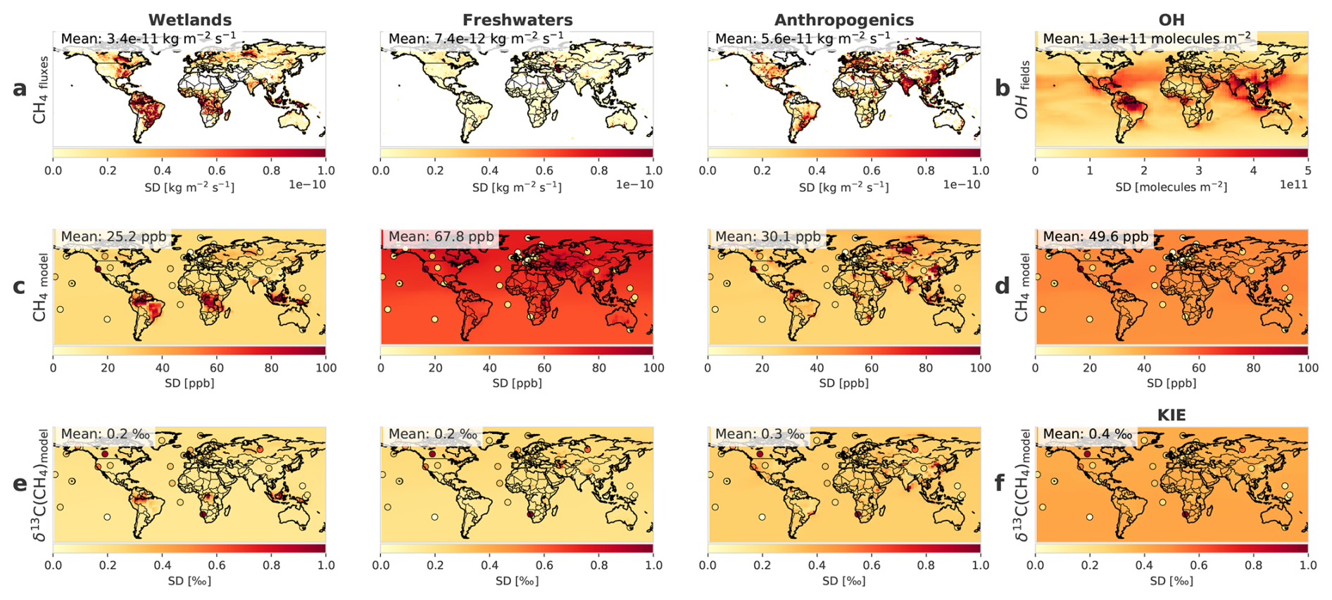
Figure 6 Standard deviation (SD) over 2016–2020. (a) SD (in $\mathrm{kg}{\mathrm{m}}^{-\mathrm{2}}{\mathrm{s}}^{-\mathrm{1}}$) of CH₄ emissions from wetlands, freshwaters, and anthropogenic sectors (AGW, FFG, BB) at surface level. Values are only displayed when the associated CH₄ flux exceeds 0.2 $\mathrm{mg}{\mathrm{CH}}_{\mathrm{4}}{\mathrm{m}}^{-\mathrm{2}}{\mathrm{d}}^{-\mathrm{1}}$. (b) SD (in $\mathrm{molec}.{\mathrm{m}}^{-\mathrm{2}}$) of the total tropospheric OH column (pressure levels below 250 hPa). (c) SD (in ppb) of CH₄ mole fractions at surface level from forward model outputs, driven by uncertainty in emission fluxes. Coloured circles indicate RSD of observed CH₄ mole fractions at surface stations with co-located δ¹³C(CH₄) measurements. (d) Same as (c), but driven by uncertainty in OH fields. (e) SD (in ‰) of δ¹³C-CH₄ values at surface level from forward model outputs, driven by uncertainty in emission fluxes. Coloured circles indicate RSD of observed δ¹³C-CH₄ values at the same stations (Michel et al., 2024; Schuldt et al., 2025). (f) Same as (e), but driven by uncertainty in kinetic isotope effects (KIE) during CH₄ oxidation.

Methane flux uncertainties are highest for anthropogenic sources (mean RSD of 129 %), followed by wetlands (96 %) and freshwaters (22 %) (Fig. S5a in the Supplement). These differences arise from inventory discrepancies, the inherent complexity of methane emission processes (e.g. large spatio-temporal variability, dependence on environmental conditions and management practices), and the uneven availability of observational data across regions and sectors, which limits the capacity to constrain emissions. Among anthropogenic subsectors, fossil fuels exhibit the largest uncertainty (RSD 83.8 %, Fig. S6), driven by inconsistent national reporting, the use of variable emission factors, and the presence of poorly constrained super-emitters (Lauvaux et al., 2022; Saunois et al., 2025). Waste emissions follow (RSD 51.9 %), and include landfills, agricultural waste, and wastewater. The limited spread across inventories for landfills is mostly due to the use of similar Tier 1 methods and data sources, not better emission constraints. Substantial uncertainties persist due to variations in emissions arising from different climate conditions, landfill management practices, and the inherent temporal and geographical variability of landfill emissions (Krautwurst et al., 2017; Nisbet et al., 2019, 2020; Bourn et al., 2019; Wang et al., 2023). Wastewater emissions remain particularly uncertain due to variability in treatment processes and limited measurements (Saunois et al., 2025). Biofuel burning shows a high RSD (55.7 %) but low absolute impact due to its smaller flux. Agriculture (RSD 42.2 %) contributes significantly in absolute terms due to its large emissions. Regarding natural sources, wetland emission uncertainties stem from multiple factors: inconsistent wetland extent maps (Melton et al., 2013; Bohn et al., 2015), uncertainties in methane production and oxidation modeling (Knox et al., 2021), and the influence of environmental drivers such as temperature and water table depth (Tian et al., 2010; Poulter et al., 2017). The dominant source of long-term uncertainty is wetland areal extent (Poulter et al., 2017; Karlson and Bastviken, 2023), while seasonal variability is primarily driven by meteorology (Parker et al., 2022; McNicol et al., 2023). Tropical wetlands remain particularly uncertain due to sparse data coverage despite their importance for global feedbacks (Nisbet, 2023; Zhang et al., 2023; France et al., 2022). Freshwater emissions are also uncertain due to poorly mapped inland waters, complex seasonal dynamics, and diverse emission pathways (e.g. diffusion, ebullition, plant-mediated transport) (Van Bergen et al., 2019; Lauerwald et al., 2023; Saunois et al., 2025). However, as only one freshwater dataset was available the sensitivity shown here reflects the introduction of freshwater emissions into the simulation (ON/OFF comparison) rather than a quantified uncertainty across multiple estimates.

Panel (c) of Fig. 6 shows how flux uncertainties propagate into modeled CH₄ mole fractions. The strongest sensitivity is linked to freshwater emissions, with an average variability of 68 ppb (4.4 %). This reflects a significant contribution to total methane emissions (+53 Tg CH₄ yr⁻¹) and strong regional impacts, particularly near the Caspian Sea, where freshwater sources dominate and where no wetland or oceanic fluxes were present in the reference simulation, thus amplifying the local sensitivity (Fig. S2). The Caspian Sea is a large endorheic saline lake whose emissions are treated as freshwater in our framework given the absence of a dedicated dataset; its brackish nature and proximity to major oil and gas infrastructure introduce additional uncertainty in this region. Anthropogenic fluxes contribute to a variability of 30 ppb (2.4 %), especially in major fossil fuel production regions such as Siberia and industrialized areas like Eastern China. Wetland fluxes result in a variability of 25 ppb (1.7 %), concentrated in high-emission regions such as the Amazon, Southeast Asia, and the Congo Basin.

Similarly, modeled δ¹³C-CH₄ signals (panel e) show a spatial pattern that mirrors CH₄ mole fraction sensitivity. Wetland and freshwater flux uncertainties both lead to an average isotopic variability of 0.2 ‰ (0.9 %), while anthropogenic fluxes cause 0.3 ‰ (1.6 %). These findings emphasize that sectoral flux uncertainties substantially influence regional isotopic signal, particularly in areas with high methane emissions.

Observed SDs from surface monitoring sites (shown as colored circles) are also displayed in panels (c) and (e) for comparison. In several cases, modeled isotopic sensitivities exceed the observed SD, especially for freshwater, induced CH₄ variability, highlighting their relevance for inversion performance (see Sect. 4.3.2). As illustrated in panels (c) and (e), the maps convey two layers of information: regional hotspots where large uncertainties may hamper local flux attribution (e.g. Caspian region, Chinese industrial basins, Congo wetlands, etc.), and background sensitivity over well-mixed or remote areas, which are critical for constraining hemispheric to global budgets. This distinction is further discussed in Sect. 4.3.2.

In summary, freshwater fluxes dominate the CH₄ mole fraction sensitivity, followed by anthropogenic and wetland fluxes. For δ¹³C-CH₄, anthropogenic fluxes induce the largest variability, with wetland and freshwater contributions of similar order. Sectoral flux uncertainties produce both regional hotspots (Caspian, Congo, Chinese basins) and broader background sensitivities, both relevant for inversion design.

4.2.3 Sensitivity to atmospheric chemistry parameters

Figure 6 also illustrates the uncertainties related to atmospheric chemistry parameters, focusing mainly on the kinetic isotope effect (KIE) of methane oxidation by tropospheric hydroxyl radicals (OH), which are the primary oxidant of methane. Panel (b) presents the SD of the total tropospheric OH column (pressure levels below 250 hPa), highlighting regions with the largest OH uncertainties. Panel (d) shows how these uncertainties affect modeled CH₄ mole fractions at surface level. Panel (f) displays how uncertainty over KIE impacts atmospheric δ¹³C-CH₄ signals. OH uncertainty does not affect δ¹³C-CH₄ signal, and OH-KIE does not impact CH₄ mole fractions. Figure S4 shows the same information in terms of RSD.

Uncertainties in OH fields (Fig. 6b and Fig. S5b in the Supplement) are substantial (e.g. Nicely et al., 2017; Collins et al., 2017; Zhao et al., 2019; Stevenson et al., 2020). SD are particularly high over tropical continental regions such as Amazonia, South Asia, and the African savannas, where OH concentrations peak due to intense photochemistry and high humidity and where strong inter-model differences coexist (Zhao et al., 2019). These regions also display marked longitudinal contrasts in tropospheric OH, driven by zonal asymmetries in convection, lightning NO_x, and biomass burning, which are not consistently captured across global chemistry models (Zhao et al., 2019; Morgenstern et al., 2025). Recent studies further suggest that tropospheric oxidative capacity is itself evolving over time: Morgenstern et al. (2025) infer an increasing global OH abundance from radiocarbon monoxide (¹⁴CO) observations, with implications for the interpretation of recent CH₄ trends (Ciais et al., 2026; Nisbet and Manning, 2026). Satellite-based observations have also been explored as a means to better characterize tropospheric OH distributions and reduce these uncertainties (Penn et al., 2025).

The sensitivity of simulated CH₄ mole fractions to OH variability (Fig. 6d) is relatively uniform globally, with an average SD of 49.6 ppb (RSD of 3.6 %). This confirms that the oxidative sink is a dominant factor controlling methane concentrations and that its uncertainties propagate broadly rather than being confined to specific regions (Zhao et al., 2019; Ciais et al., 2026; Belikov et al., 2026; Nisbet and Manning, 2026; Skeie et al., 2023). While OH-related uncertainties propagate globally and uniformly, their impact near source regions appears limited (Fig. 6d). This is particularly relevant given ongoing concerns about CH₄–OH interactions in polluted areas, where local nonlinearities may arise due to complex dependencies of OH concentrations on emissions of NO_x, CO, and volatile organic compounds (VOCs) (Lin et al., 1988; Guthrie, 1989; Holmes et al., 2013; Lelieveld et al., 2016; Gaubert et al., 2017). In theory, elevated CH₄ concentrations could partially saturate the OH sink, especially in regions with high levels of co-emitted VOCs and NO_x that alter oxidative capacity. However, this expected nonlinearity is not strongly expressed in the CH₄ sensitivity maps. Because OH concentrations are prescribed and do not respond to CH₄ levels in our configuration, the oxidative capacity is higher than it would be under interactive chemistry. This conservative setup further dampens any potential CH₄–OH saturation effects, explaining the relatively uniform CH₄ sensitivity patterns shown in Fig. 6d. Moreover, the SD induced by OH variability exceeds the observed SD of CH₄ mole fractions at most monitoring sites, indicating that OH-related uncertainties alone can introduce model variability greater than observational noise.

Regarding the kinetic isotope effect, Figs. 6f and S5f in the Supplement show that uncertainties in the OH-KIE induce a geographically homogeneous SD of 0.4 ‰ (RSD of 2.2 %) in the atmospheric δ¹³C-CH₄ signal, exceeding the observed SD at surface stations (Michel et al., 2024; Schuldt et al., 2025). This sensitivity is driven by only two published experimental determinations of the ${}^{\mathrm{12}}\mathrm{C}/{}^{\mathrm{13}}\mathrm{C}$ KIE for CH₄+OH: Cantrell et al. (1990) (1.0054±0.0009 at 296 K) and Saueressig et al. (2001) (1.0039±0.0004 at 296 K). No measurements exist below 278 K, although theoretical calculations suggest the KIE may increase at lower temperatures (Gupta et al., 1997). At steady state, Fujita et al. (2020) showed that the 0.0015 difference between the two values yields a ∼1.3 ‰ shift in atmospheric δ¹³C-CH₄, illustrating the high leverage of this parameter. In practice, previous inversions have adopted either value, Saueressig et al. (2001) in e.g. Nisbet et al. (2016); Schaefer et al. (2016); Basu et al. (2022); Thanwerdas et al. (2024), and Cantrell et al. (1990) in e.g. Rice et al. (2016). This choice is absorbed by the posterior source mixture. Accordingly, we recommend treating the full Cantrell–Saueressig range in inversion frameworks (see Sect. 4.3.2).

Beyond OH, two additional sinks contribute to the δ¹³C-CH₄ budget and deserve explicit discussion: oxidation by chlorine (Cl) and soil uptake. Both are included in our forward simulations (Sect. 3.2) but were not perturbed in dedicated sensitivity experiments.

The Cl sink accounts for a small fraction of total CH₄ oxidation. Recent estimates converge on a tropospheric contribution of ∼1 %–3 % of the total chemical sink (Hossaini et al., 2016; Sherwen et al., 2016; Gromov et al., 2018; Wang et al., 2021), with the latest Global Methane Budget reporting a climatological tropospheric Cl sink of 6 [1–13] Tg CH₄ yr⁻¹ (Saunois et al., 2025), substantially smaller and better constrained than earlier estimates (Allan et al., 2007). Despite this small magnitude, the Cl reaction carries an exceptionally large kinetic isotope effect (KIE ≈1.066 at 298 K; Saueressig et al., 1995), more than an order of magnitude larger than that of OH, so even modest uncertainties in Cl concentrations translate into substantial shifts in modeled δ¹³C-CH₄ (see Table 2). Basu et al. (2022) further identified the combined uncertainty in fractionation (OH-KIE and Cl contribution) as the single most important factor limiting isotope-based source partitioning at the global scale (Röckmann et al., 2024). Thanwerdas et al. (2022b) quantified this influence within the same CIF-LMDz-SACS framework used here, and reported a near-linear sensitivity of +11.7 Tg CH₄ yr⁻¹ and −1.0 ‰ in the globally averaged source signature per 1000 $\mathrm{molec}.{\mathrm{m}}^{-\mathrm{3}}$ increase in mean tropospheric Cl, with stratospheric Cl alone contributing a ∼0.30 ‰ surface enrichment via stratosphere–troposphere exchange and modifying the δ¹³C-CH₄ seasonal cycle amplitude by up to 10 %–20 % depending on latitude. Because our configuration adopts the Cl field from Wang et al. (2021), consistent with the most recent tropospheric chlorine chemistry, the Cl-related uncertainty in our simulations is bounded by the ranges quantified in Thanwerdas et al. (2022b), which are of the same order of magnitude as the OH-KIE sensitivity reported in Table 6. A dedicated Cl sensitivity experiment was therefore not repeated here to avoid duplicating a recent and comprehensive analysis with the same model.

Soil uptake contributes ∼31 [17–39] Tg CH₄ yr⁻¹ to the global CH₄ budget (Saunois et al., 2025), or about 5 % of the total CH₄ sink, with a moderate KIE of ∼1.020 (Snover and Quay, 2000), intermediate between OH (1.0039) and Cl (1.066) (see Table 2). In our framework, it is implemented as a first-order deposition process with isotope-dependent deposition velocities (Sect. 3.1.5). Given its small relative contribution to the total sink, its moderate KIE, and the well-constrained global magnitude reported in recent budgets, soil uptake uncertainties are expected to have a substantially smaller impact on the modeled δ¹³C-CH₄ signal than the OH-KIE (Table 6), and were therefore not perturbed in the Monte Carlo ensemble.

In summary, OH-KIE is the dominant chemistry-related driver of δ¹³C-CH₄ variability, while OH fields dominate CH₄ mole fraction sensitivity. The Cl sink also exerts a strong leverage on δ¹³C-CH₄ through its large KIE; its impact within the same CIF-LMDz-SACS framework has been comprehensively quantified by Thanwerdas et al. (2022b) and is therefore not duplicated here.

4.2.4 Sensitivity of simulated atmospheric δ¹³C-CH₄ to source signatures

Figures 7 and S8 in the Supplement present the sensitivity of the simulated atmospheric δ¹³C-CH₄ signal to uncertainties in source-specific isotopic signatures, based on the Monte Carlo simulations (see Sect. 3.2). Panel (a) displays the SD of the prescribed δ¹³C-CH₄ source signatures used as input to the simulations. The highest signature RSDs are associated with the BB sector, with an RSD of 36 % and a SD of 7.8 ‰, followed by FFG sector (RSD: 13.0 %, SD: 6.1 ‰), NAT sector (RSD: 12.0 %, SD: 5.3 ‰), WET sector (RSD: 9.2 %, SD: 5.2 ‰), and AGW sector (RSD: 7.3 %, SD: 4.6 ‰). These RSD values are consistent with the sector-specific uncertainty ranges summarized in Table S3. The spatial pattern of these uncertainties reflects the regional sampling domains used in the Monte Carlo parameterization (see Sect. 3.2).

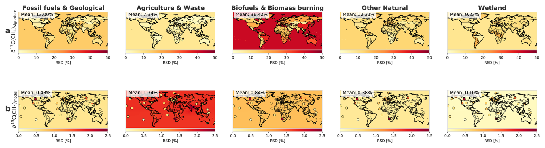
Figure 7 (a) SD (in ‰) of the δ¹³C-CH₄ source signature sensitivities inputs for Monte Carlo simulations, by sector at surface level. (b) SD of the δ¹³C-CH₄ source signal from Monte Carlo simulations, by sector at surface level. Coloured circles indicate RSD of observed δ¹³C-CH₄ values at each surface station over the study period (Michel et al., 2024; Schuldt et al., 2025).

Panel (b) shows the resulting variability in modeled atmospheric δ¹³C-CH₄ at surface level. These simulations only perturb the isotopic composition of the emissions while keeping total CH₄ fluxes fixed, as a result, there is no corresponding effect on CH₄ mole fractions. Despite having a comparatively lower SD in its source signature, the AGW sector emerges as the dominant driver of atmospheric δ¹³C-CH₄ uncertainty, with a mean sensitivity of 0.32 ‰ (1.74 %). This impact is particularly pronounced in regions with high AGW emissions, such as India, where EDGARv8 estimates an annual mean emission of 26 Tg CH₄ per year over the period 2016–2020. Other sectors contribute less significantly to overall isotopic variability but still have regionally relevant effects: BB contributes 0.16 ‰ (0.84 %), FFG 0.04 ‰ (0.43 %), NAT 0.07 ‰ (0.38 %), and WET 0.02 ‰ (0.10 %).

Uncertainties in source-specific isotopic signatures, particularly from AGW sector, translate into substantial variability in the simulated δ¹³C-CH₄ signal. This effect is especially pronounced in emission hotspots, where even small shifts in isotopic assumptions can significantly affect local atmospheric signals. Conversely, background regions remain sensitive to these uncertainties through long-range transport, potentially biasing hemispheric or global source attribution. Moreover, the mean RSD induced by AGW source signature uncertainties (1.74 %) exceeds the observed RSD of δ¹³C-CH₄ at most surface stations, suggesting that this parameter is a major limiting factor for isotopic inversions. For other sectors (e.g. BB, FFG, NAT), the simulated RSD remains generally closer to or below observed values, depending on the station location and the local sensitivity to each source's isotopic signature. These findings underscore the need to improve isotopic characterization of agricultural and waste-related methane sources, especially in hotspots regions. Implications for the design and configuration of such systems are discussed in Sect. 4.3.2.

In summary, AGW source signature uncertainties dominate isotopic variability despite a moderate input SD, due to the large flux of this sector. BB, FFG, NAT and WET signature uncertainties have comparatively limited atmospheric impact at the global scale but produce regionally important effects. Improving AGW isotopic characterization, particularly in emission hotspots, is the highest-priority lever for source-signature-related uncertainty reduction.

Our sensitivity analysis shows that uncertainties in the OH kinetic isotope effect (KIE) are the dominant drivers of variability in the modeled δ¹³C-CH₄ signal at global scale. Uncertainties in agriculture and waste sector source signatures and fluxes also contribute significantly. In contrast, uncertainties associated with fossil fuel and wetland source signatures, as well as those related to fluxes used for aggregation, have a more limited impact at the global level (more details in Sect 4.3.1).

4.3 Discussion

This section discusses the key outcomes of the sensitivity analysis (Sect. 4.3.1) and their implications for atmospheric methane inversions (Sect. 4.3.2). We examine how the sensitivity analysis results can inform the configuration of isotopic inversions, particularly regarding uncertainty specification and parameter prioritization. The main objective is to distinguish between uncertainty components that could be reduced through improved input data or model structure, and those that are intrinsic and must be explicitly optimized within the inversion framework (see Fig. 4). Finally, we identify opportunities for future improvements, both within inversion systems and through supporting efforts such as inventories, field campaigns, and process-based models (Sect. 4.3.3).

4.3.1 Key uncertainty drivers affecting CH₄ and δ¹³C-CH₄ simulations

This section synthesizes the sensitivity results presented in Sect. 4.2 and identifies the dominant drivers of uncertainty in modeled CH₄ mole fractions and δ¹³C-CH₄ signals. Figure 8 provides an integrated overview, locating each tested parameter according to its joint impact on both quantities. Parameters in the upper-right quadrant induce the largest uncertainties simultaneously in CH₄ and δ¹³C-CH₄ and therefore represent priority targets for model improvement. As detailed in Sect. 4.2, freshwater fluxes and OH fields dominate CH₄ variability, while OH-KIE and AGW source signatures dominate δ¹³C-CH₄ variability. Aggregation choices, as well as FFG, BB, NAT and WET source signatures, exert a comparatively limited influence at the global scale. These findings are consistent with previous work identifying OH-KIE as a primary limitation for isotopic source partitioning (Basu et al., 2022; Chandra et al., 2024), and extend earlier analyses by quantifying the additional contribution of interannual variability in OH fields, wetland and freshwater fluxes, and isotopic source signatures.

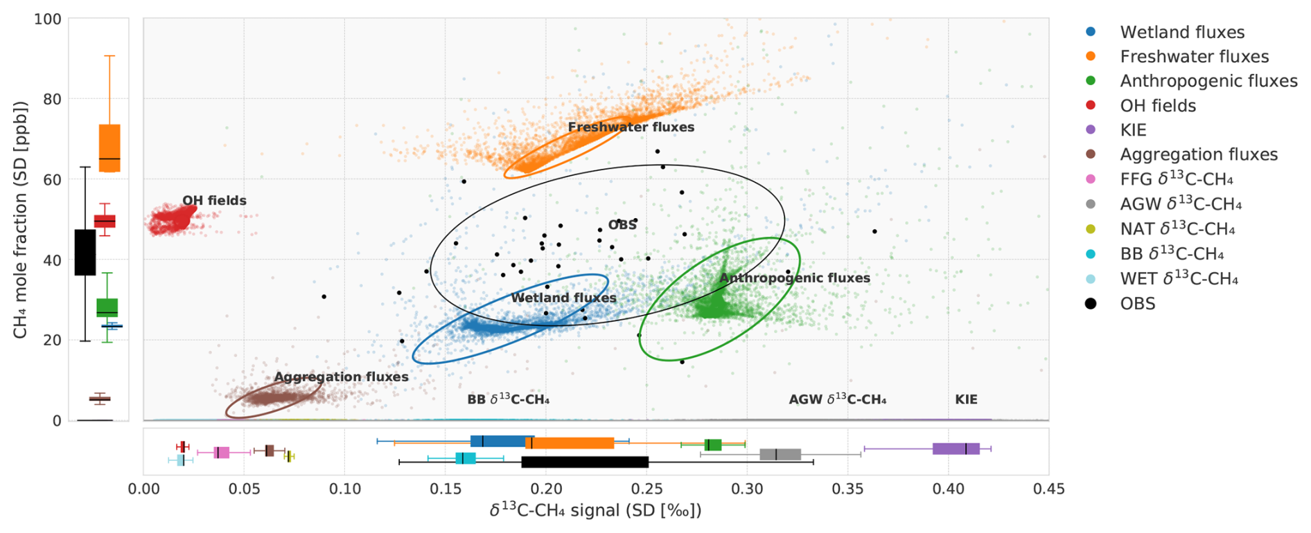
Figure 8 Uncertainties in CH₄ mole fraction and the δ¹³C-CH₄ isotopic signal across various parameters. The x axis shows the SD of CH₄ mole fractions in parts per billion (ppb), while the y axis shows the SD of the δ¹³C-CH₄ signal in per mil (‰). Each point represents a simulated grid cell, and the point labeled OBS corresponds to observations from a surface monitoring station. Parameters located in the upper-right quadrant induce the largest uncertainties in both mole fraction and isotopic composition.

To assess whether these modeled sensitivities are large enough to matter for inversion frameworks, they must be compared to the natural variability captured by atmospheric observations. The observed standard deviation of surface CH₄ mole fractions reaches 44 ppb, while that of δ¹³C-CH₄ is 0.23 ‰ (Fig. S8). Several parameters tested here exceed these thresholds: freshwater fluxes and OH fields for CH₄, and OH-KIE, AGW source signatures and wetland fluxes for δ¹³C-CH₄. This means that the uncertainties associated with these parameters are not absorbed by observational noise and propagate directly into inversion outcomes. The magnitude of these uncertainties is also non-negligible relative to the long-term atmospheric trends used to interpret methane budget changes, namely $+\mathrm{9.4}\pm \mathrm{0.3}$ ppb yr⁻¹ for CH₄ over 2016–2020 (Lan et al., 2025) and approximately −0.04 ‰ yr⁻¹ for δ¹³C-CH₄ (Schuldt et al., 2025), reinforcing the need for explicit treatment in inversion configurations.

Figure 9 illustrates the spatial distribution of the dominant source of uncertainty in each grid cell, complemented by Fig. S9 and S10 in the Supplement which provide a detailed quantification of the contribution of each parameter to the total variance of the simulated δ¹³C-CH₄ signal and CH₄ mole fraction at the model grid cell level. Beyond globally aggregated diagnostics, this spatial classification reveals a strongly heterogeneous structure, with OH-KIE dominating δ¹³C-CH₄ variance over most of the globe (around 50 % of total variance) and regional exceptions emerging in well-defined emission hotspots. Four regional case studies illustrate the diversity of dominant drivers and provide context for the targeted improvements discussed in Sects. 4.3.2 and 4.3.3.

• Indo-Gangetic Plain: AGW source signatures contribute up to 80 % of the local δ¹³C-CH₄ variance over this region. This dominance reflects both the magnitude of regional AGW emissions (∼26 Tg CH₄ yr⁻¹ from EDGARv8 over 2016–2020) and the strong isotopic contrast between livestock (−65.8 ‰) and waste sub-sectors (−50.9 to −56.2 ‰). The relative livestock share varies from 67 % (EDGARv8) to 79 % (CEDS, GAINS), directly generating the spread observed in atmospheric simulations. Resolving this hotspot requires improved partitioning between livestock and waste sub-sectors in regional inventories, complemented by isotopic measurements that capture C₃$/$C₄ dietary heterogeneity. The Ethiopian highlands provide a finer-scale illustration of this need: the C₃$/$C₄ forage balance varies with altitude, producing sub-national contrasts in livestock signatures (Brychkova et al., 2022) that current global inventories cannot resolve. Emerging evidence from dual-isotope (δ¹³C–δD) measurements over South Asia (e.g. Yao et al., 2026) suggests that AGW emissions in this region may carry distinct isotopic fingerprints from co-located fossil fuel sources, supporting the use of multi-isotopic constraints for source disentanglement in densely emitting tropical regions.

• Tropical wetlands (Congo Basin, Amazon, Borneo): Wetland flux uncertainties dominate over these regions, reaching more than 60 % of local δ¹³C-CH₄ variance in Borneo. These regions host some of the largest global wetland emissions but remain critically under-sampled. Recent tropical airborne and ground-based campaigns (France et al., 2022; Nisbet et al., 2021; Shaw et al., 2022) have begun addressing this gap, reporting signatures broadly consistent with those used here but covering only a limited number of sites. Sustained measurement programs in these basins are essential to constrain both flux magnitudes and isotopic signatures of tropical wetland emissions.

• Caspian region: Freshwater flux uncertainties account for more than 60 % of the local δ¹³C-CH₄ variance. The Caspian Sea is a large endorheic brackish lake, treated here as a freshwater source given the absence of a dedicated dataset for endorheic systems; this classification ambiguity, combined with proximity to major oil and gas infrastructure in Turkmenistan and Azerbaijan, makes regional source attribution particularly challenging. More broadly, freshwater emissions remain poorly constrained due to complex emission pathways and limited mapping of inland water extent (Lauerwald et al., 2023; Saunois et al., 2025).

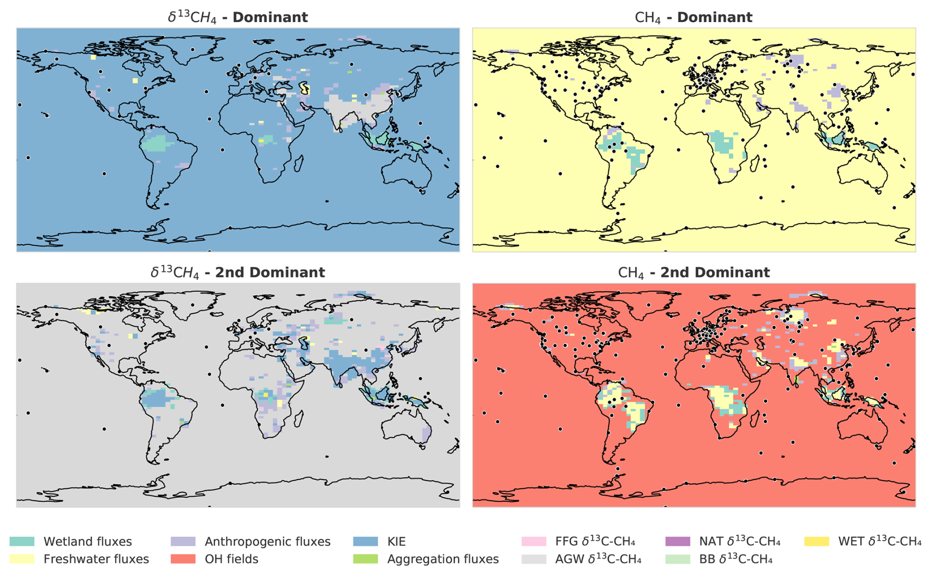
Figure 9 Spatial distribution of the dominant uncertainty driver (parameter with the highest RSD) in each grid cell at the surface. The second row of plots shows the dominant uncertainty category after removing the primary driver from the analysis. Surface stations are indicated with black dots.

The second row of Fig. 9 highlights the secondary drivers that would emerge if first-order uncertainties were reduced, with anthropogenic and freshwater fluxes becoming critical in many additional regions. Together, these case studies support a key conceptual distinction between two regimes of uncertainty: localized hotspots, where large uncertainties hinder source attribution at the regional scale and where targeted external efforts (inventories, field campaigns, process models) can reduce prior errors; and remote or well-mixed background regions, where uncertainties are dominated by OH-KIE and propagate through long-range transport, requiring explicit optimization within the inversion framework. The implications of this distinction for inversion design, including B and R matrix specification, are detailed in Sect. 4.3.2.

4.3.2 Implications for isotopic inversions

The sensitivity results synthesized in Sect. 4.3.1 directly inform the design of isotopic inversions. The central question is how to allocate effort between two complementary strategies: reducing prior uncertainties through external inputs (inventories, process models, field campaigns), and explicitly optimizing intrinsic uncertainties within the inversion framework. Thanwerdas et al. (2022b) previously emphasized the need for spatially explicit, sectorally disaggregated uncertainty assessments to guide this allocation, and the present study fills this gap through an ensemble of forward simulations.

Reducible uncertainties primarily concern AGW source signatures, freshwater fluxes, and wetland fluxes, which dominate in localized hotspots (Sect. 4.3.1). They can be addressed through external efforts complementary to inversion development: expanded inventories with finer spatial and sectoral resolution, dedicated isotopic field campaigns, and refined process-based models. The risk of co-located sources with overlapping signatures, previously highlighted by Drinkwater et al. (2023), reinforces the need for these external efforts: without them, unresolved prior uncertainties propagate into the inversion and lead to ambiguous source attribution (Fig. 4).

Intrinsic uncertainties, primarily related to the OH-KIE, cannot be reduced through prior refinement and must instead be sampled within the inversion framework via ensemble-based or variational approaches, unless laboratory or theoretical advances narrow the Cantrell–Saueressig range. This recommendation aligns with Lan et al. (2021a) and addresses a gap identified by Basu et al. (2022) and Thanwerdas et al. (2024), namely the lack of robust, data-driven uncertainty estimates for source signatures and KIE in current δ¹³C-CH₄ inversions.

The sectoral total uncertainties σ_total reported in Table 4 provide a quantitative basis for specifying the diagonal terms of the prior error covariance matrix B. The sensitivity ranges quantified in Sect. 4.2 similarly inform the model–observation mismatch component of the observation error matrix R when source signatures or KIE are held fixed. The relative magnitude of B and R determines whether each parameter can be effectively constrained: when B≫R and the parameter has a detectable atmospheric signature, the inversion reduces uncertainty significantly; when B≪R, the posterior remains close to the prior. These relationships, schematized in Fig. 4 and extended to the isotopic case in Fig. 10, provide the rationale for the configuration choices recommended below. Where observations are sparse, particularly in the Southern Hemisphere, spatial clustering based on isotopic similarity may improve inversion stability.

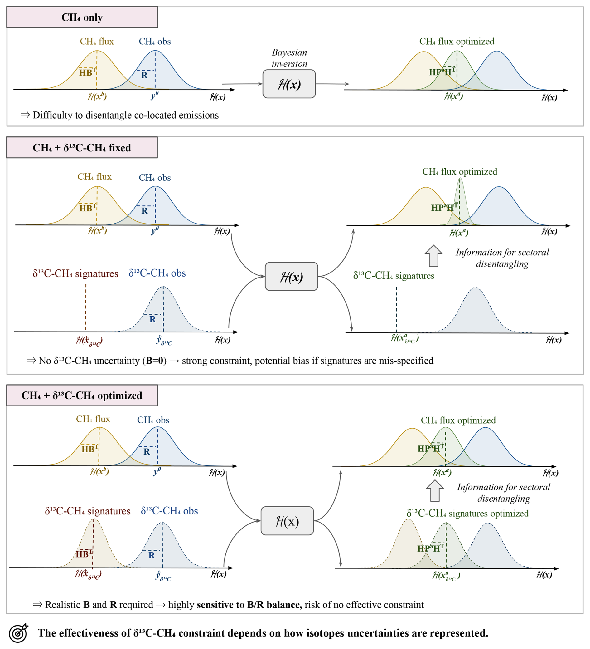
Figure 10 Schematic illustration of the effect of adding δ¹³C-CH₄ constraints in the inversion. The upper panel shows the reference case using CH₄ only, where co-located emissions are difficult to disentangle. The middle panel illustrates the case where δ¹³C-CH₄ signatures are fixed with no uncertainty (B=0), which provides a strong constraint but may lead to potential biases if the signatures are mis-specified. The lower panel shows the case where δ¹³C-CH₄ signatures are optimized with realistic uncertainties, which improves the ability to disentangle emission sectors but requires a careful balance between B and R to avoid ineffective constraints. Coloured Gaussian curves represent prior, observational and posterior distributions for CH₄ fluxes and δ¹³C-CH₄ signatures, with the forward model ℋ(x) linking the parameter space to the observation space.

Several practical recommendations emerge from this framework:

• AGW sectoral granularity: Within the AGW sector, livestock and waste sub-sectors carry strongly contrasted signatures (Table 1) and should not be merged into a single category, in agreement with Menoud et al. (2022) and Mannisenaho et al. (2023). The five sub-sector structure used here is sufficient at the global scale (Sect. 4.2.1, NO_AGGREG test), but the livestock–waste distinction must be preserved in inversion priors. Within this five sub-sector structure, the dominant AGW contribution to atmospheric δ¹³C-CH₄ uncertainty (Sect. 4.2.4, Table 6) originates from uncertainty on the sub-sector signature values themselves, not from how they are aggregated; this should guide the specification of the prior error covariance matrix for AGW signatures.

  Freshwater treatment: Freshwater fluxes have a strong CH₄ signature but remain poorly constrained. Including them within an extended wetland category, rather than as a separate optimized source, may currently offer the best trade-off until more observational data become available. Omitting them entirely would bias regional attribution, particularly in Central Asia and the tropics.

• OH treatment: Although OH does not affect δ¹³C-CH₄ directly, it propagates strongly into CH₄ mole fraction variability and should be incorporated through chemistry ensemble fields rather than fixed climatologies.

• Aggregation transferability: The minor sensitivity to aggregation choices (Sect. 4.2.1) supports the use of the isotopic maps developed here across diverse inversion systems and emission inventories, provided sub-sector heterogeneity within AGW is preserved.

These recommendations build on and quantify the qualitative needs identified by Basu et al. (2022) and Thanwerdas et al. (2024), and provide a directly usable basis for configuring the next generation of δ¹³C-CH₄ inversions.

4.3.3 Pathways for improvement

Beyond the inversion configuration choices discussed in Sect. 4.3.2, several research directions are needed to reduce the uncertainties identified in this study. These cut across three complementary axes: temporal representativeness of source signatures, atmospheric transport and chemistry, and process-level understanding of natural emissions.

A first priority concerns the temporal dimension of isotopic signatures, which is currently held constant for most sub-sectors over 1998–2022. Documented changes in livestock feeding practices, particularly the evolving balance between C₃ and C₄ plant diets, are known to modulate ruminant δ¹³C-CH₄ signatures (Chang et al., 2019; Lan et al., 2021a) and remain insufficiently represented. Similarly, finer differentiation between waste sub-sectors (landfills, wastewater, agricultural waste) would improve AGW characterization (Menoud et al., 2022). Because seasonal variations in δ¹³C-CH₄ are particularly sensitive to small shifts in source signatures, both their amplitude and phase can be affected (Kangasaho et al., 2022), making temporal characterization a critical lever for inversion performance.

A second priority concerns atmospheric transport and chemistry, which were not perturbed in our sensitivity ensemble. All simulations were performed with LMDz at a single resolution (Sect. 3.1.1), and the TransCom-CH₄ intercomparison (Patra et al., 2011) showed that modeled CH₄ budgets are sensitive to troposphere–stratosphere exchange rates and to vertical grid structure, with CH₄ lifetimes spanning 9.50–10.27 yr across 12 CTMs using identical OH fields. For δ¹³C-CH₄, vertical transport additionally controls the rate at which ¹³C-enriched stratospheric air re-enters the troposphere via the Brewer–Dobson circulation, as well as the vertical distribution of the Cl sink and its strong fractionation (Butchart, 2014; Thanwerdas et al., 2022b). The sensitivity hierarchy identified here, dominated by OH-KIE and AGW signatures, is driven by prescribed inputs and is expected to be robust across CTMs, but quantifying transport-related uncertainty through multi-model ensembles remains a priority. In parallel, additional oxidation pathways deserve dedicated attention: emerging evidence for previously unaccounted-for Cl sources, notably photocatalytic release from mineral dust–sea spray aerosol (van Herpen et al., 2023; Röckmann et al., 2024), and the potential of novel tracers such as δ¹³C-CO to detect regional Cl-driven oxidation, should be considered in future isotopic inversion setups.

A third priority concerns process-level understanding of natural emissions. Wetland and freshwater methane emission models suffer from limited data on hydrological dynamics, organic matter content, and microbial population dynamics, particularly in tropical regions where the largest emissions coincide with the sparsest observations. Coordinated airborne and ground-based campaigns, exemplified by MOYA and ZWAMPS in tropical wetlands, rice fields, and biomass burning regions (Nisbet et al., 2021; France et al., 2022), provide a model for the type of effort needed to fill these observational gaps. Enhanced national reporting of sectoral emissions, particularly for waste and agriculture, and site-specific isotopic measurements in major fossil production basins and under-sampled freshwater systems are equally needed to constrain prior fluxes and signatures.

Together, these three axes define a research agenda complementary to inversion development itself: without parallel progress on temporal characterization, transport and chemistry, and process-based understanding, isotopic inversions will remain limited by the very priors they aim to constrain.

5 Code and data availability

Isotopic source signature datasets were provided by Xin Lan, Malika Menoud, Youmi Oh, and Giuseppe Etiope. The gridded δ¹³C-CH₄ source signature dataset (1998–2022) developed in this study is openly available under CC BY 4.0 at the ESA Open Science Data portal (Tapin et al., 2025, https://doi.org/10.57780/ESA-6D202E9). The atmospheric modeling framework used for the sensitivity analysis is based on the Community Inversion Framework (CIF; Berchet et al., 2021, https://doi.org/10.5194/gmd-14-5331-2021) coupled to the LMDz transport model. The dataset is provided at two levels of sectoral granularity to accommodate different modeling needs. The aggregated product contains gridded monthly δ¹³C-CH₄ signature maps for the five main source sectors used throughout this study (FFG, AGW, BB, WET, NAT). In addition, the disaggregated product provides gridded monthly δ¹³C-CH₄ signature maps for each of the 13 underlying sub-sectors (coal, oil and gas, geological, livestock, wastewater, landfills, agricultural waste, rice, biofuel burning, biomass burning, wetlands, termites, oceans). Users can therefore re-aggregate the dataset using their own sectoral classification or their preferred flux inventory, in line with the framework described in here. Scripts used for dataset processing and uncertainty analysis are available upon request from the corresponding author.

6 Conclusions

Existing global δ¹³C-CH₄ datasets (e.g. Lan et al., 2021a; Oh et al., 2022; Menoud et al., 2022; Thanwerdas et al., 2024) have provided valuable benchmarks but were limited in temporal coverage, systematic uncertainty quantification, and compatibility with inversion-ready sectoral structures. To address these limitations, we produced an updated global dataset of δ¹³C-CH₄ source signatures for five major natural and anthropogenic sectors, following the Global Methane Budget (GMB) classification. This aggregation strategy reduces the number of categories for computational efficiency in future inversion studies while preserving isotopic representativeness across emission types. The maps cover the period 1998–2022 and integrate recent spatially explicit datasets and literature-derived observations, providing explicit estimates of both intrinsic (within-sector) and aggregation-related uncertainties. Overall, this new dataset offers a temporally extended, uncertainty-quantified, and inversion-ready basis for atmospheric modeling and isotopic inversions. To support a broad range of inversion configurations, the dataset is distributed at two levels of sectoral granularity: the five-sector aggregated product used in this study, and the underlying 14 sub-sector maps, allowing users to re-aggregate according to their own classification or flux-weighting scheme.

Using forward simulations in the Community Inversion Framework coupled to the LMDz transport model, we conducted a comprehensive sensitivity analysis to assess the influence of key parameters on the modeled atmospheric δ¹³C-CH₄ signal and CH₄ mole fraction. Our results highlight that uncertainties in methane oxidation chemistry, particularly related to the OH kinetic isotope effect (KIE), and uncertainties in isotopic source signatures, especially from the agriculture and waste (AGW) sector, have the largest impact on the simulated isotopic ratios. By contrast, uncertainties related to flux aggregation, fossil fuel (FFG), wetland (WET) and other natural (NAT) isotopic source signatures have a more limited influence on global atmospheric signals.

We showed that isotopic uncertainties within certain sectors, such as the AGW sector (up to ±3 ‰), were substantial when compared to the standard deviation of atmospheric δ¹³C-CH₄ observations at surface stations (approximately ±0.2 ‰). This emphasizes the importance of reducing uncertainties in source-specific signatures and isotopic fractionation processes to improve the reliability of atmospheric inversions.

Our results demonstrated the robustness of the proposed sector aggregation approach and confirmed the applicability of the updated isotopic maps across diverse inversion configurations. We recommend prioritizing efforts to better constrain isotopic signatures in the agriculture and waste sector, and to refine the OH kinetic isotope effect. Moreover, the methodology presented here for quantifying sectoral δ¹³C-CH₄ uncertainties can be applied to future datasets as new observations become available, allowing the isotopic maps to be updated and the associated uncertainties reduced. In addition, we provide practical guidelines for configuring isotopic inversions, including recommended uncertainty ranges, key parameters to target for enhanced source attribution, and the use of regional optimization strategies in areas where uncertainties are most significant. The sectoral uncertainty estimates provided here can directly inform the specification of prior error covariance matrices in atmospheric inversion frameworks, thereby improving the consistency between sensitivity analyses and inversion configurations.

This study focused on developing and evaluating updated δ¹³C-CH₄ source signature maps through comparison with the literature, uncertainty quantification, and forward simulations. While direct validation using atmospheric data is beyond the scope of this paper, all necessary elements are provided, including gridded maps, uncertainty ranges, and sectoral breakdowns, to enable their integration into forward modeling and atmospheric inversions under optimal conditions.

Finally, the increasing availability of satellite-based CH₄ and isotopic measurements opens promising perspectives for constraining methane sources at the global scale. Feasibility studies (Malina et al., 2018, 2019) have shown that instruments such as GOSAT-2, TROPOMI, and Sentinel-5/UVNS could in principle retrieve ¹³CH₄, but several technical limitations currently prevent routine isotopic retrievals. Individual ¹³CH₄ retrieval uncertainties remain large: Malina et al. (2019) report mean uncertainties of <1 ppb for TROPOMI (SWIR3 channel) and <0.68 ppb for Sentinel-5/UVNS (SWIR1 channel), whereas the target δ¹³C uncertainty of <1 ‰ required to differentiate between source types corresponds to a ¹³CH₄ uncertainty of <0.02 ppb. Significant spatial and/or temporal averaging is therefore required to reduce uncertainties to detectable levels. In addition, ¹³CH₄ retrievals are highly sensitive to errors in a priori temperature and pressure profiles, which can introduce systematic biases (Malina et al., 2019). A dedicated detectability assessment will be essential to evaluate whether current or forthcoming missions can effectively detect and interpret atmospheric isotopic variations under real conditions.