Oceanographic dataset of the near-shore water column of the northeastern Gulf of St. Lawrence, Canada, during the ice-free season

Coastal ecosystems are highly dynamic and vulnerable to both climate changes and anthropogenic pressures. The Sept-Îles region, located in the northwestern Gulf of St. Lawrence, is a high-use subarctic coastal system with diverse urban, industrial and maritime activities. This study presents analyses of monthly water column profiles at 35 sites focusing on temperature, salinity and chlorophyll fluorescence, used as a proxy of phytoplankton biomass, during the ice-free season. Using a conductivity, temperature and depth (CTD) probe, water column profiles were collected from May to October 2022 along the coastline, at sites between 2 and 52 m depth. Results revealed a thermocline developing in spring, intensifying in summer and disappearing in autumn. Chlorophyll a (Chl a) concentrations peaked below the thermocline in July, while secondary increases were recorded at the surface in September, consistent with observations of an autumn bloom in similar environments. These findings highlight the complex dynamic of physical and biological variables in the coastal water column, and the importance of the timing of sampling to fully capture seasonal variability. To improve future research in the area, measuring nutrient concentrations would be essential for detecting potential upwelling events and better explaining phytoplankton variation during summer. This study provides a valuable baseline for future investigations and justifies the continuation of measurements of water column variability in the region, in the context of rapid climate change. The complete dataset is available via https://doi.org/10.5683/SP3/ALRWON (Arseneault and Saulnier-Talbot, 2025a).

1 Introduction

Coastal environments are at the forefront of climate change impacts, experiencing diverse types of alterations due to rising global temperatures and anthropogenic activities (IPCC, 2023). These changes are noticeable in the Gulf of St. Lawrence, where sea ice cover has declined markedly over the past decade (Galbraith et al., 2024a). This trend, linked to rising winter air temperatures over the past few decades, highlights the region's sensitivity to global warming, which is expected to lead to increasingly ice-free conditions in the near future (Galbraith et al., 2024a). The Sept-Îles region, located in the northwestern Gulf of St. Lawrence, represents an economically vital area, hosting the most important mineral port in North America (PSI, 2025). Because of its industrial importance, the area is susceptible to several anthropogenic drivers (Beauchesne et al., 2020), in addition to rapid climatic changes. Among these, the disappearance of seasonal sea ice is the most evident (Allard et al., 2025). In an effort to better understand the changing dynamics of the coastal ecosystem, several biodiversity studies are being conducted in the region's aquatic environment, covering diverse topics such as benthic communities (Dreujou et al., 2020; Joshi et al., 2025), intertidal and coastal diatoms (Arseneault et al., 2023; Arseneault and Saulnier-Talbot, 2025b), algal and bacterial pigments (Lefebvre, 2023; Araújo et al., 2022), microbial _sedDNA (Bélanger, 2024), and sea ice ecology (Allard et al., 2025). Regular environmental monitoring has also been undertaken (Carrière et al., 2018a; Ferrario et al., 2022), and the Bay of Sept-Îles (BSI) is currently part of the Enviro-Actions program, allowing a near real-time monitoring of industrial port zones (Carrière and Dreujou, 2024). In this context, understanding the hydrological characteristics of the Sept-Îles region (Shaw et al., 2022) and the dynamics of the water column is crucial for tracking the variability, rate, direction and intensity of environmental change over time.

Among the most significant features of the water column, the thermocline, a water layer at which temperature decreases rapidly with depth, plays a key role in regulating stratification. This division of the water column into different layers can create barriers for organisms (Fiedler, 2010). Seasonal stratification regulates phytoplankton dynamics, with spring blooms commonly observed in temperate waters, including the BSI (Roden and Raine, 1994; Araújo et al., 2022; Lim et al., 2025). Most studies focusing on water column layers are usually carried out in deeper areas, far from the coast (de Boyer Montégut et al., 2004; Galbraith, 2006). However, evidence of stratified water columns in shallow coastal areas has also been documented. For example, on the west coast of Ireland, stratification within 10 km of the shore was observed (Roden and Raine, 1994) and in southern waters of Korea, thermal stratification was found to occur at sites between 5 and 30 m depths (Lim et al., 2025). Despite these findings, studies on shallow-water stratification remain scarce.

Given the combination of climatic and direct anthropogenic pressures in this region, documenting baseline physical and biological conditions in the coastal water column is essential for assessing potential ecological changes that could affect the food web and impact ecosystem services, such as fisheries and tourism. Establishing this baseline is also important for future monitoring and management initiatives, including the “Chaire de recherche sur les écosystèmes côtiers et les activités portuaires, industrielles et maritimes” (or EcoZone Chair, at Université Laval), which seeks to improve knowledge on coastal ecosystem functioning and to ensure sustainable management of these ecosystems subjected to urban, port, industrial and maritime activities.

The objective of this study was to characterize the spatial and seasonal dynamics of the near-shore water column in the Sept-Îles region during the ice-free season. We aimed to (1) describe monthly vertical profiles between May and October 2022, of temperature, salinity, turbidity, and in vivo chlorophyll a fluorescence; (2) examine spatial and temporal patterns of these key oceanographic parameters; and (3) identify thermocline structure and fluorescence patterns to better understand how temperature and primary production co-vary in this region throughout the ice-free season.

2 Material and methods

2.1 Study area

The study area covers the coastline of the Sept-Îles region, between 66°56^′ N and 65°54^′ W (Fig. 1). Situated in the northwestern Gulf of St. Lawrence, this region features a mix of saltwater brought by the Atlantic Ocean and freshwater from the St. Lawrence River and its tributaries (Carrière et al., 2018b). The region is under a semi-diurnal tidal system where tides range between 0.39 to 3.6 m in Port-Cartier and 0.43 to 3.36 m in Sept-Îles (Fisheries and Ocean Canada, 2024). The area has a subarctic climate and has historically been covered by sea ice between November and April (Aubut Demers et al., 2018). However, this period has been shrinking rapidly, and nearly ice-free winters could become more common due to climate warming (Galbraith et al., 2024a). Since 2010, the Gulf of St. Lawrence has experienced 4 winters with nearly ice-free conditions around the end of the season (Galbraith et al., 2024a).

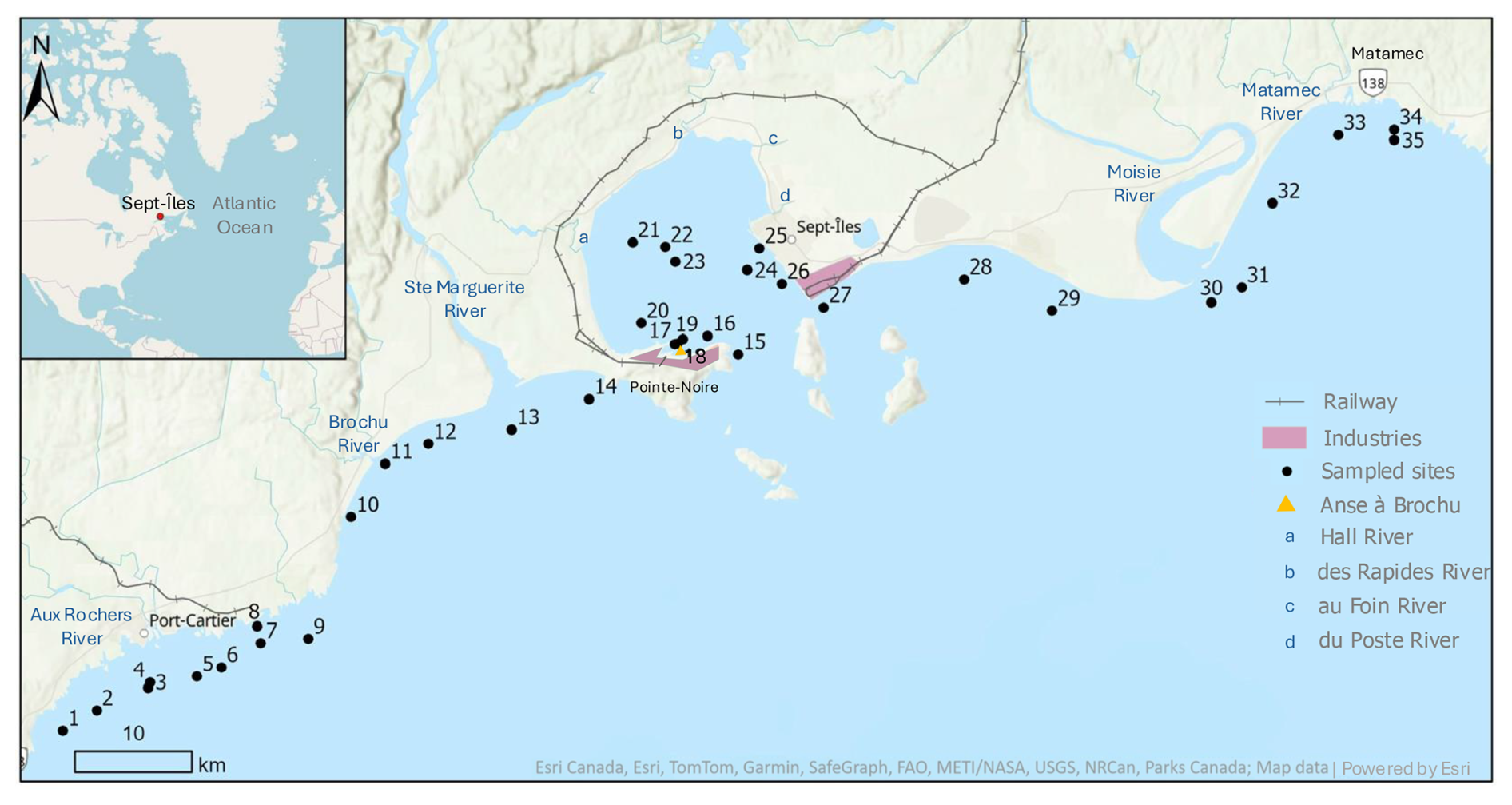
Figure 1 Map of the location of the 35 sites sampled around Sept-Îles and the major rivers of the region.

According to a study on the hydrodynamics of the BSI (Shaw et al., 2022), the area exhibits an estuarian circulation pattern. Currents are seaward at the surface (2–10 m) and shoreward in deeper waters (10–30 m). Surface drifter measurements indicate average and maximum speeds of 17.4 and 86.6 cm s⁻¹, respectively. While locally dominated by tides, currents in the bay result from complex interactions between tides, estuarine circulation, winds, and the Earth's rotation. Water residence time is estimated to be 5.6 ± 3.5 d.

Diverse types of land-use along the transect were observed: natural coastlines with less developed areas, residential areas (urban and suburban) and Industrial-Port (IP) Zones. Sites 5 to 8 in Port-Cartier are located in an IP zone, and the Port of Sept-Îles (PSI) is the second largest Canadian port for annual activity (PSI, 2025) where several heavy industries contribute to the economic importance of the region. The Matamec sector presents a less developed and more pristine environment, featuring an ecological reserve and the Matamec River, which is of great conservation value (Government of Quebec, 2011). The study area is affected by freshwater input from the Ste-Marguerite and Moisie rivers, damned and wild, respectively. Smaller rivers also flow in the area, including the rivière aux Rochers in Port-Cartier and Brochu River, West of the Ste-Marguerite. The Hall, des Rapides, aux Foins and du Poste rivers flow into the BSI, with around 22 m³ s⁻¹ of freshwater input into this area annually (Shaw, 2019).

2.2 Water sampling

The vertical profiles were obtained with a Conductivity-Temperature-Depth (CTD) probe equipped with sensors that measure temperature and salinity (Sea-Bird Electronics SBE19plusV2), photosynthetically active radiation (PAR; Biospherical QSP-2300L with a spherical quantum sensor), turbidity (Seapoint) and in vivo chlorophyll fluorescence (Seapoint). The sensors were last calibrated in 2017, so the data should be interpreted with caution and considered as relative rather than absolute values. Fluorescence was used as an indicator of phytoplankton chlorophyll a biomass (Chl a). Chl a is an indicator of phytoplankton biomass and reflects the level of primary production in coastal waters (Araújo et al., 2022). The CTD was equipped with an integrated software system that automatically calculated practical salinity, density, specific volume anomaly, Brunt-Väisälä frequency, Sigma-T, potential temperature, Sigma-Theta, freezing temperature, sound velocity, and absolute salinity. At each site, the CTD was lowered to approximately 2–3 m above the seafloor to prevent potential damage to the instrument and had an average descent speed of 1 m s⁻¹ and a sampling frequency of 4 Hz Measurements along the transect were made monthly at all sites between May and October 2022 (24–26 May, 14–15 June, 19–21 July, 16–17 August, 13–14 September and 24 October), except at site 34 in May and site 25 in June due to technical problems. The full dataset is available at https://doi.org/10.5683/SP3/ALRWON (Arseneault and Saulnier-Talbot, 2025a). Meteorological data for the week prior to sampling was also documented using data from the Government of Canada (2025) (Table A1). To facilitate visualizations, the 35 sites were divided into three Zones (Table 1). Sites 1 to 15 between Port-Cartier and the west of the BSI were defined as Zone 1, sites inside the BSI (16 to 27) were defined as Zone 2, and Zone 3 encompasses the sites from the east of the BSI to Matamec (28 to 35). Monthly vertical profiles of temperature, salinity, turbidity and fluorescence at each site were generated using “ggplot” (R core Team, 2022). With the same statistical package, relationships between Chl a and environmental variables were explored. Scatter plots with LOESS curves to observe general trends were generated and Spearman correlation was used to assess the significance of these relationships. A summary of the variables measured in the surface water of the three site zones for each month of sampling is available in the annex (Table A2).

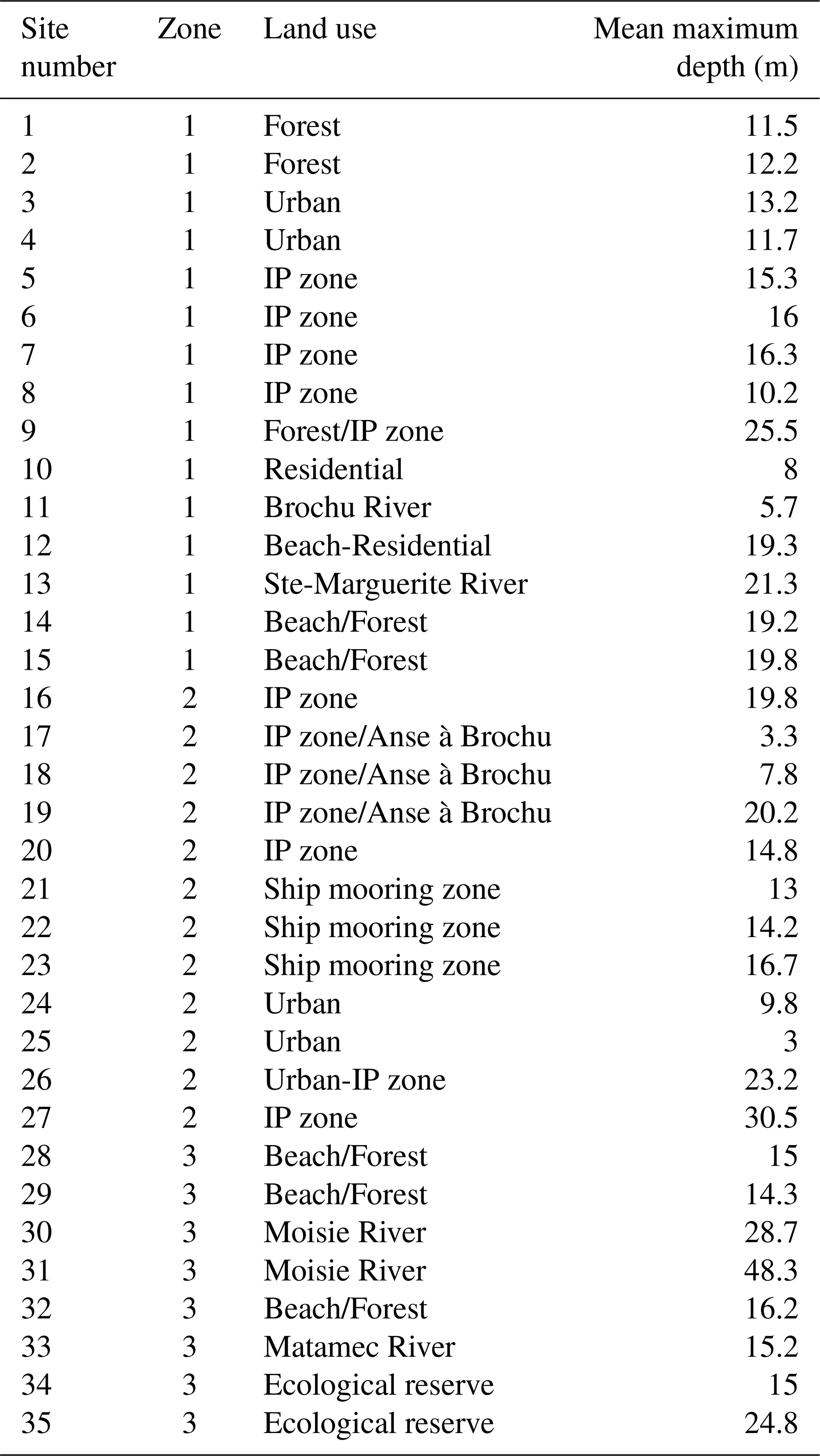
Table 1 Site zones, description of land use, and mean of the maximum CTD depth for each site (Zone 1 = Sites between Port-Cartier and the west of the BSI; Zone 2 = Sites inside the BSI; Zone 3 = Sites between the east of the BSI and Matamec; IP = Industrial-port zone).

2.3 Water column structure and light attenuation

Thermocline layers were identified, if possible, monthly at every site. Determining the depths of the thermocline is not always straightforward, as several methods can be used (de Boyer Montégut et al., 2004). These methods are however rarely applied in areas as shallow as in this study. Janecki et al. (2022) found no studies of this sort except in the Baltic Sea, where depths still reached 100 m (Leppäranta and Myrberg, 2009). These authors developed a new algorithm for shallow seas to find the top of the thermocline and halocline, for sites reaching >100 m. We decided for this study to use the gradient threshold method of 0.2 °C (de Boyer Montégut et al., 2004; Leppäranta and Myrberg, 2009). We assumed that the top layer of the thermocline was located at the depth of the strongest gradient of the slope (ΔT>0.2 °C), and the lower layer was located at the depth of the deepest gradient, to capture the typical plateau, if there was one. Since the sites in our study area were shallow, between 4 and 52 m with an 18 m median, we decided to start the calculations at 3 m depth instead of the advised near-surface 10 m depth (de Boyer Montégut et al., 2004). This approach also avoided the possible effects of the instrument, the anchor and the boat, which can mix the surface waters (de Boyer Montégut et al., 2004; Maske et al., 2014). The depths of the thermocline layer were obtained with the package “rLakeAnalyzer” (Winslow et al., 2019), with some modifications of the “therm.depth” function. A cutoff of 1 °C was also applied, a default criterion in the R function. If the change between surface and maximum depth temperatures was less than this threshold, thermocline depth was not calculated. Thermocline depths were not calculated for sites with a maximum depth <5 m. The same gradient threshold method was applied to salinity and density profiles to identify the halocline and pycnocline. We chose to use temperature in the present study as a primary indicator of vertical stratification, consistent with recent studies that have focused on the thermocline in similar environments with dynamic coastal waters influenced by water masses and anthropogenic activities (Lim et al., 2025, and references therein). The euphotic depth was also calculated using the depth at which PAR declined to 1 % of the surface value (Kirk, 1994), and the stratification index as the density difference (kg m⁻³) between the maximum sampled depth and the surface (3 m) sampled depth levels (Blais et al., 2019). The diffuse attenuation coefficient K_d (PAR) (m⁻¹) was calculated for each CTD profile using linear regression of the natural log of PAR against depth, following Lund-Hansen (2004). Profiles with a maximum depth <5 m, or r²<0.8 were excluded. Simple and multiple linear regressions were then performed between K_d and depth-averaged in vivo fluorescence and turbidity to examine the drivers of light attenuation. One site out of the 35 was chosen to illustrate seasonal changes in the vertical profiles of temperature, salinity, Chl a and PAR during the sampling season.

3 Results

3.1 Temperature and thermocline

In May, the water temperature was the coldest and was mostly even across depth at all sites (Fig. 2). Surface temperature averaged 5.56 °C along the transect. At maximum depth, temperatures ranged between 0.85 °C (Site 31) and 3.83 °C (Site 11), excluding site 25 which was only 3 m deep. During this period, a near-surface thermocline was beginning to form (Figs. 2 and 3), usually between 3 and 4 m depth (Table A3). In May, 22 sites showed the onset of stratification. In June, surface temperatures began to rise, ranging from 8.69 °C (site 32) to 11.99 °C (site 19). The water column remained largely mixed, but stratification became noticeable at deeper sites, such as sites 9, 27 and 31, where temperatures were between 1.72 °C (Site 31) and 4.3 °C (Site 9) at maximum depth. Sixteen sites exhibited thin thermocline layers (1–2 m thick), mostly near the bottom of the water column. Waters in June were generally well-mixed.

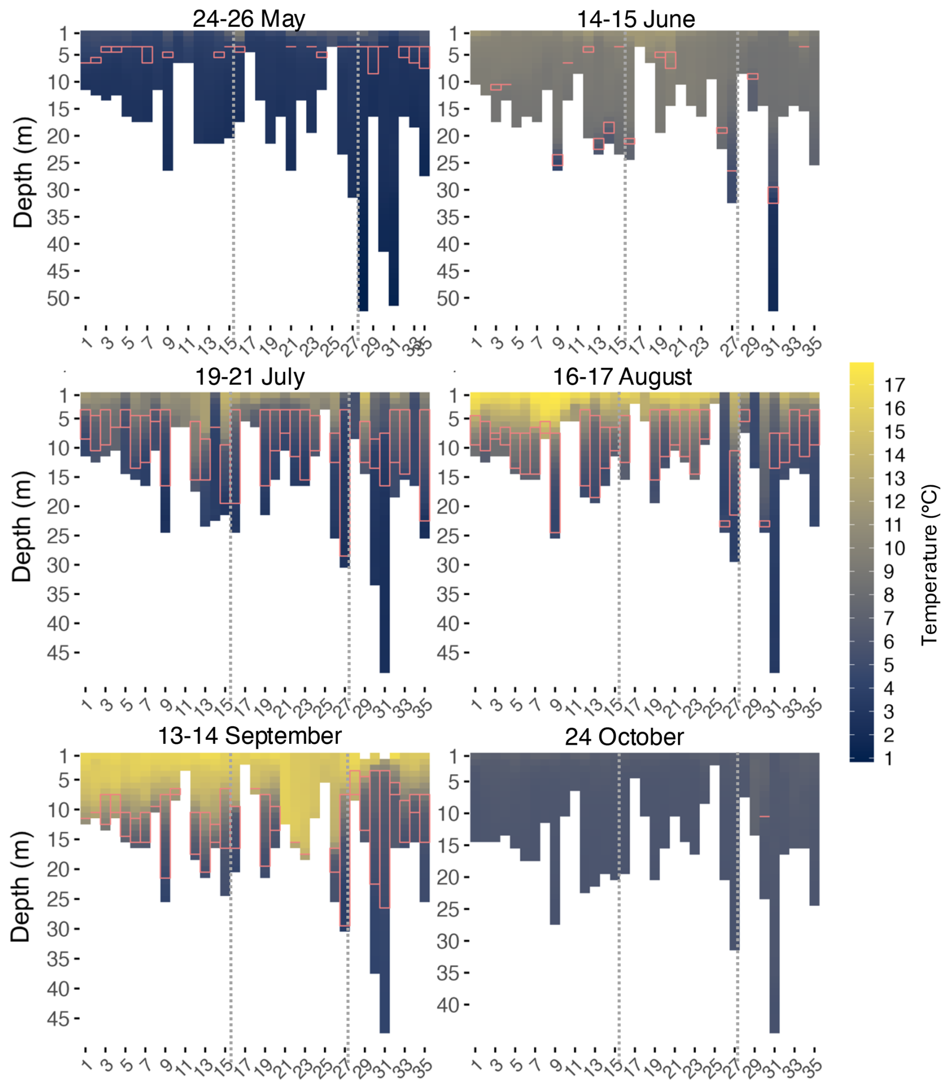
Figure 2 Temperature heatmaps for every month at every site (x axis) along the transect. Dotted lines indicate division of Zones 1 (West), 2 (BSI), and 3 (East), from left to right. The pink rectangles represent the thickness of the thermocline layer.

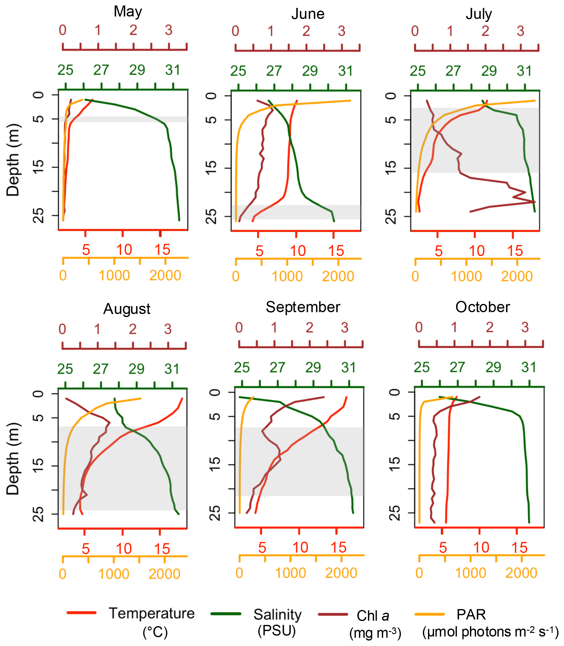
Figure 3 Vertical profiles of temperature, salinity, Chl a and PAR at Site 9, on each sampling date. The gray box represents the thermocline layer.

Between July and September, clear stratification developed with increasing temperatures, though a few shallow sites, <6 m depth, lacked distinct layers. At most sites in July, a thermocline was observed between 4 and 5 m depth. Surface temperatures ranged from 5.52 °C (Site 28) to 14.80 °C (Site 29). While surface warming was observed at some sites, 14 sites recorded a colder surface temperature than in June. For instance, recorded temperature at site 34 was 10.15 °C in June versus 5.63 °C in July. Temperature became colder at shallower depths in July, contrasting with June's well mixed conditions where colder waters only appeared at the deepest sites. In August, surface temperatures ranged between 5.18 °C (Site 29) and 17.92 °C (Site 9). Stratification was still persistent but started to deepen. August showed a deepening of the thermocline: up to 4 m at some sites (5 and 6) in the west, while sites in the BSI, like sites 19 to 24, showed the same depth layers as in June. At the eastern sites, the thermocline deepened between 4 and 12 m. September marked the warmest month throughout the water column, although deeper sites like sites 31, 30 and 9 retained colder bottom temperatures, around 4.2 °C. At several western sites, the thermoclines continued to deepen, while they began to disappear at the BSI sites and became shallower toward the east, near the Moisie River (sites 30 and 31). By October, the entire transect showed uniform temperatures with no significant differences between surface and maximum depths, and the absence of a thermocline. In early fall, the overall mean surface temperature was 6.83 °C, with 5.55 °C at maximum depth, resulting in an average difference of only 1.28 °C throughout the water column. All sites were mixed, except for site 31, the deepest one, that showed a weak persistent thermocline at around 10 m depth. The stratification index confirmed this trend, with mean values peaking in August and September (2.9 km m³) and dropping in October (0.7 km m³) across all zones (Table A3).

In summary, surface temperatures increased from May to September, with stratification becoming prominent in July. By October, conditions in the transect had reversed back to cold, uniform temperatures across depths. The largest changes in surface temperatures occurred between May and June (increase of 5.02 °C), and September and October (a decrease of 9.30 °C). Site 9 was chosen as an example (Fig. 3) to show how the thermocline layer, using the threshold method, matched with the vertical profiles of temperature and other parameters. This site was approximately 25 m deep and had no missing values, which made visualization easier. At this specific site, the thermocline, as observed in general, started to appear in May at a shallow depth, deepened during summer and disappeared in October.

3.2 Salinity

Signals of freshwater input at sites near river mouths were apparent in May (Fig. 4), particularly at sites 29 (17.8 PSU), 31 (19.7 PSU) and 30 (20.1 PSU), located near Moisie River. These sites recorded the lowest surface salinity, likely due to increased volume of river discharge following spring snowmelt. The overall average salinity of the water column in May was 30.0 PSU. Despite this localized freshwater influence, thermocline, halocline and pycnocline depths were closely aligned in May, within approximately 1 m at most sites (Table A3). June recorded an average of 27.8 PSU, the lowest salinity of the season. Thermocline and halocline depths differed among zones. In Zone 2, the halocline (5.3–10.9 m) occurred above the thermocline (14.9–16.1 m), suggesting that stratification was mostly driven by surface salinity associated with freshwater inputs. In contrast, in Zone 3, the halocline (20.5 m) was deeper than the thermocline (13.8–15.2 m). Halocline and pycnocline were aligned in all 3 zones in June. July showed the highest salinity with an average across sites around 30.6 PSU. Stratification became more visible at some sites in July where salinity was lower above the thermocline, such as sites 13 and 15, that recorded 28 PSU versus 30 PSU below. In August, salinity above the thermocline decreased to around 27 PSU, showing the deepening of stratification. A strong signal of freshwater input by rivers was again observed in September, this time near the Brochu and Ste-Marguerite rivers, at sites 11 (17.6 PSU) and 12 (19.1 PSU). Between July and September, the onset depths of thermocline, halocline, and pycnocline were generally aligned, but the thermocline extended deeper, resulting in a thicker thermally-stratified layer compared to the halocline and pycnocline. In October, salinity was more uniform below the surface, while surface salinity remained lower, especially at sites located west of the transect, where salinity at Site 1 reached 20 PSU at the surface. Below surface, salinity increased to over 30 PSU along the water column. Although the thermocline was absent across the transect by October, the halocline and pycnocline remained detectable at some sites. Throughout the study period, halocline and pycnocline depths were mostly aligned (Table A3), indicating that salinity had more influence on density stratification in the water column, especially in June.

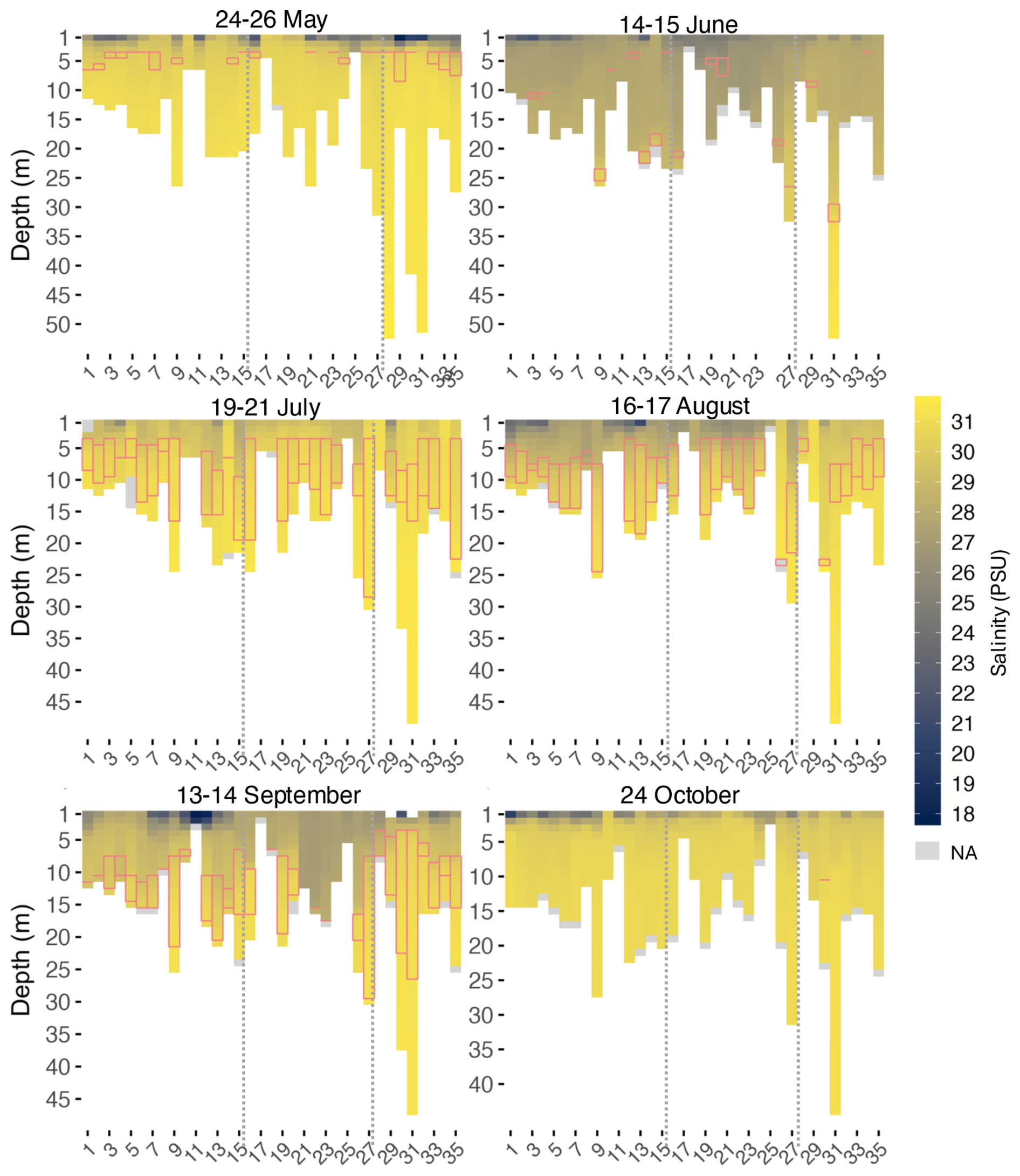
Figure 4 Salinity heatmaps for every month at every site (x axis) along the transect. Dotted lines indicate division of Zones 1 (West), 2 (BSI), and 3 (East), from left to right. The pink rectangles represent the thickness of the thermocline layer.

In these data, salinity inversely followed temperature trends in the water column, where it increased with depth while temperature decreased. This relationship was visible in vertical profiles such as Site 9 (Fig. 3). A Spearman correlation analysis confirmed that temperature and salinity were inversely correlated across the dataset ($r=-\mathrm{0.84}$, p value<0.01). Overall, salinity at maximum depth showed little seasonal variation, averaging over 30 PSU, except in June (28.5 PSU). The most pronounced seasonal differences in salinity were observed at surface. May and June had the lowest surface salinities whereas July had the highest salinity, and August only showed a slight decrease, in general. A drop in surface salinity was observed in September, especially at sites near the Brochu River (Site 11). Salinity exhibited variability at the surface (first 2 m), usually at sites located near rivers, and became uniform at depth.

3.3 Turbidity

Because turbidity mostly varied at surface, only data down to a depth of 5 m was shown for better clarity (Fig. 5). Turbidity across the transect varied between 0 and 8.4 Formazin Turbidity Units (FTU) with limited variability, except at certain sites mostly located inside the BSI (sites 16 to 21). These sites showed a turbidity range of 4.8 to 8.4 FTU, with the highest value measured at site 20.

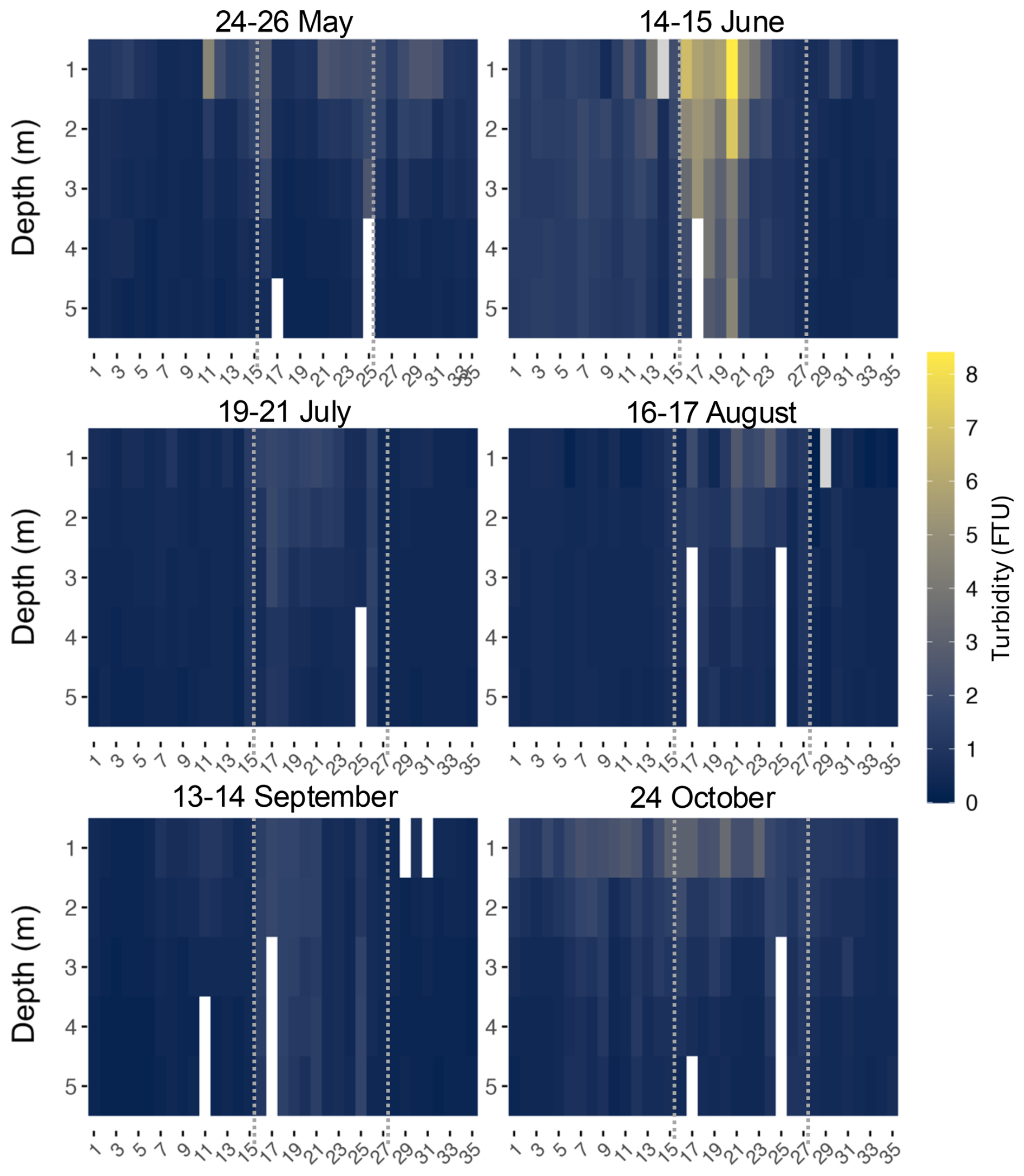
Figure 5 Turbidity heatmaps for every month at every site (x axis) along the transect. Dotted lines indicate division of zones 1 (West), 2 (BSI), and 3 (East), from left to right.

Higher values of turbidity, superior to 2 FTU, were also recorded in May, in the BSI and at sites near river mouths, such as sites 11 (4.6 FTU), 30 and 31. A similar pattern was observed in October, with higher turbidity values in the BSI and at sites close to rivers, where Site 20 exhibited a surface turbidity of 3.2 FTU and Site 11 a turbidity of 2.6 FTU. In July and September, turbidity remained below 2 FTU throughout the transect, with sites within the BSI being slightly more turbid than the others.

3.4 Fluorescence (Chl a) and PAR

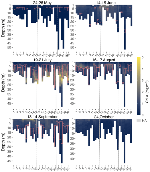
A seasonal variation of fluorescence (Fig. 6), reflecting concentration of Chl a, was observed along the transect.

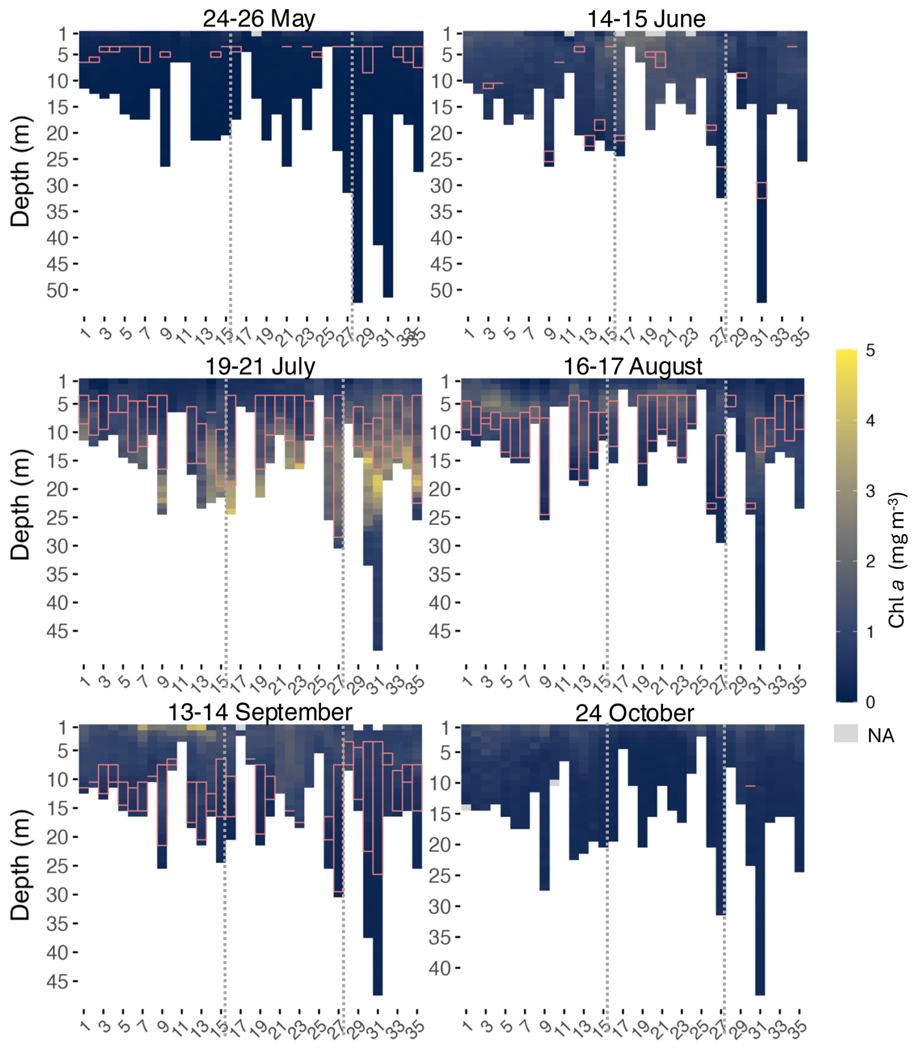
Figure 6 Chl a heatmaps for every month at every site (x axis) along the transect. Dotted lines indicate division of zones 1 (West), 2 (BSI), and 3 (East), from left to right. The pink rectangles represent the thickness of the thermocline layer.

Concentrations were the lowest in May and began to rise in June, reaching a peak in July, and then decreased throughout August to October. In September, a localized resurgence was observed at the surface of some sites, before fluorescence levels declined again in October at most sites.

In May, surface fluorescence throughout the transect averaged 0.37 mg m⁻³ and surface PAR 943.8 $\mathrm{\mu }\mathrm{mol}\mathrm{photons}{\mathrm{m}}^{-\mathrm{2}}{\mathrm{s}}^{-\mathrm{1}}$. All sites had a concentration below 1 mg m⁻³ at all depths. In June, surface fluorescence increased to a mean of 1.07 mg m⁻³, with surface PAR averaging 1517.5 $\mathrm{\mu }\mathrm{mol}\mathrm{photons}{\mathrm{m}}^{-\mathrm{2}}{\mathrm{s}}^{-\mathrm{1}}$. Sites 17, 18 and 19 recorded the highest Chl a concentration. These were the only sites across the entire transect where fluorescence exceeded 2 mg m⁻³ in June, all between 1 and 3 m. In July, a subsurface fluorescence maximum was observed at several sites, with the highest concentrations found at sites 30, 31, 16, and 35, followed by Site 23, where concentrations were all superior to 4 mg m⁻³, at depths between 15 to 24 m. All these sites were located near rivers, except for Site 16 which was positioned in front of an aluminum smelter. At this site, the highest concentration of 4.28 mg m⁻³ was measured at 24 m, which was the maximum depth at this site. All fluorescence peaks were below the thermocline layer, except at Site 35 where fluorescence concentrations were higher at the thermocline. Surface fluorescence averaged 0.53 mg m⁻³ in July, while surface PAR averaged 746.1 $\mathrm{\mu }\mathrm{mol}\mathrm{photons}{\mathrm{m}}^{-\mathrm{2}}{\mathrm{s}}^{-\mathrm{1}}$, lower than in June. August showed the highest surface PAR of the season, averaging 1707 $\mathrm{\mu }\mathrm{mol}\mathrm{photons}{\mathrm{m}}^{-\mathrm{2}}{\mathrm{s}}^{-\mathrm{1}}$, while surface fluorescence averaged 0.57 mg m⁻³. Sites 3, 4, 5, and 6, all located in Port-Cartier near the aux Rochers River estuary, and Site 31 at the Moisie River, had a concentration superior to 2 mg m⁻³. Maximum fluorescence (2.73 mg m⁻³) was observed at Site 4 at a depth of 5 m. Highest fluorescence in August occurred at shallower depths than in July, between 5 and 26 m. In contrast to July, peaks of Chl a in August were mostly found at shallower depths, either above or within the thermocline layer.

In September, surface fluorescence reached its seasonal peak, averaging 1.59 mg m⁻³, with surface PAR averaging 326.5 $\mathrm{\mu }\mathrm{mol}\mathrm{photons}{\mathrm{m}}^{-\mathrm{2}}{\mathrm{s}}^{-\mathrm{1}}$. Sites 7 (3.49 mg m⁻³), 12 (3.84 mg m⁻³) and 13 (4.06 mg m⁻³) recorded higher fluorescence concentrations than in August, all at the surface. Concentrations higher than 2 mg m⁻³ were observed at 8 sites, all located in the western part of the transect. Fluorescence declined again in October, with a mean surface of 1.11 mg m⁻³. The maximum fluorescence for this month (1.79 mg m⁻³) was measured at the surface of Site 32, followed by the surface of Site 9 (1.71 mg m⁻³).

3.5 Diffuse light attenuation coefficient; K_d (PAR)

The diffuse attenuation coefficient, K_d (PAR) ranged from 0.12 to 1.05 m⁻¹, with an overall mean of 0.32 m⁻¹, showing both seasonal and spatial variability along the transect (Fig. 7). June had the highest mean K_d (0.43 m⁻¹), where sites 18, 20, 21 and 22 reached values between 0.58 and 1.05 m⁻¹, the highest value recorded along the transect. October showed the second highest mean (0.37 m⁻¹), particularly at sites influenced by rivers such as Site 11 (0.78 m⁻¹) and Site 28 (0.68 m⁻¹), where higher turbidity was observed that month. July had the lowest mean K_d (0.24 m⁻¹), indicating clearer water conditions during the summer stratified period. Throughout all months, the eastern sites showed the lowest K_d values (0.24 m⁻¹), while the BSI had the highest (0.35 m⁻¹).

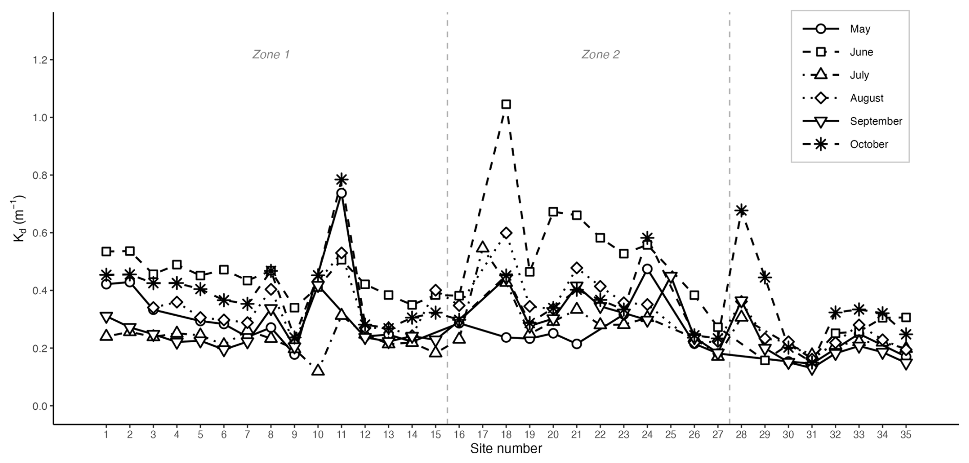
Figure 7 Diffuse light attenuation coefficient K_d at each site along the transect for the six sampling months. Dashed vertical lines delimit the three site zones.

A significant positive correlation was found between K_d and depth-averaged turbidity (r²=0.59, p<0.001), while the relationship between K_d and depth-averaged fluorescence was weak (r²=0.02, p<0.05). Fluorescence was not a significant driver when included alongside turbidity in the multiple regression (p>0.05), suggesting that turbidity, rather than phytoplankton biomass, was the dominant driver of light attenuation, consistent with the elevated turbidity values observed at BSI and river-influenced sites.

3.6 Relationship between Chl a and environmental variables (temperature, salinity, PAR and turbidity)

In this data set, temperature, salinity, turbidity and PAR all had significant effects on Chl a, and the scatterplots and LOESS smoothers revealed nonlinear relationships (Figs. 8 and A1–A4). The highest Chl a concentrations were mostly observed at colder temperatures, particularly between 1 and 5 °C, and at higher salinities between 30 and 32 PSU. However, the monthly breakdown revealed that the direction of these relationships changed across the season. In May and June, Chl a increased with temperature (r=0.89 and 0.81), while in July the relationship reversed ($r=-\mathrm{0.61}$), reflecting the subsurface fluorescence maximum where the highest concentrations occurred at deeper cold temperatures (Fig. A1). Concentrations then decreased with increasing temperature, with a secondary rise at warmer values, as suggested by the trend. This could reflect the fewer peaks of Chl a near the surface observed in autumn. A negative relationship between Chl a and salinity was observed in most months, suggesting that higher concentrations tended to occur at lower salinities, possibly linked to localized riverine inflow and associated nutrient inputs. July was an exception, where a positive relationship was observed, likely reflecting the subsurface fluorescence maximum (Fig. A2). Peaks of fluorescence were most abundant under low to moderate light conditions. When focusing on Chl a peaks only (>2 mg m⁻³), the relationship with PAR showed a weak negative correlation ($r=-\mathrm{0.46}$, p<0.01) as opposed to a weak positive one with all the data (r=0.42, Fig. 8), consistent with the subsurface fluorescence maximum observed in July (Fig. A3). This was also visible at Site 9 (Fig. 3), where in July, peaks (>3 mg m⁻³) were below the thermocline at low PAR between 19.8 and 29.2 $\mathrm{\mu }\mathrm{mol}\mathrm{photons}{\mathrm{m}}^{-\mathrm{2}}{\mathrm{s}}^{-\mathrm{1}}$. Turbidity measurements were mostly between 0 and 2 FTU during the sampling period, which coincided with most of the Chl a peaks and was positively associated with Chl a in most months (Fig. A4) Overall, the strength and direction of the relationships between Chl a and the environmental variables varied across months, highlighting the seasonal dynamics along the transect.

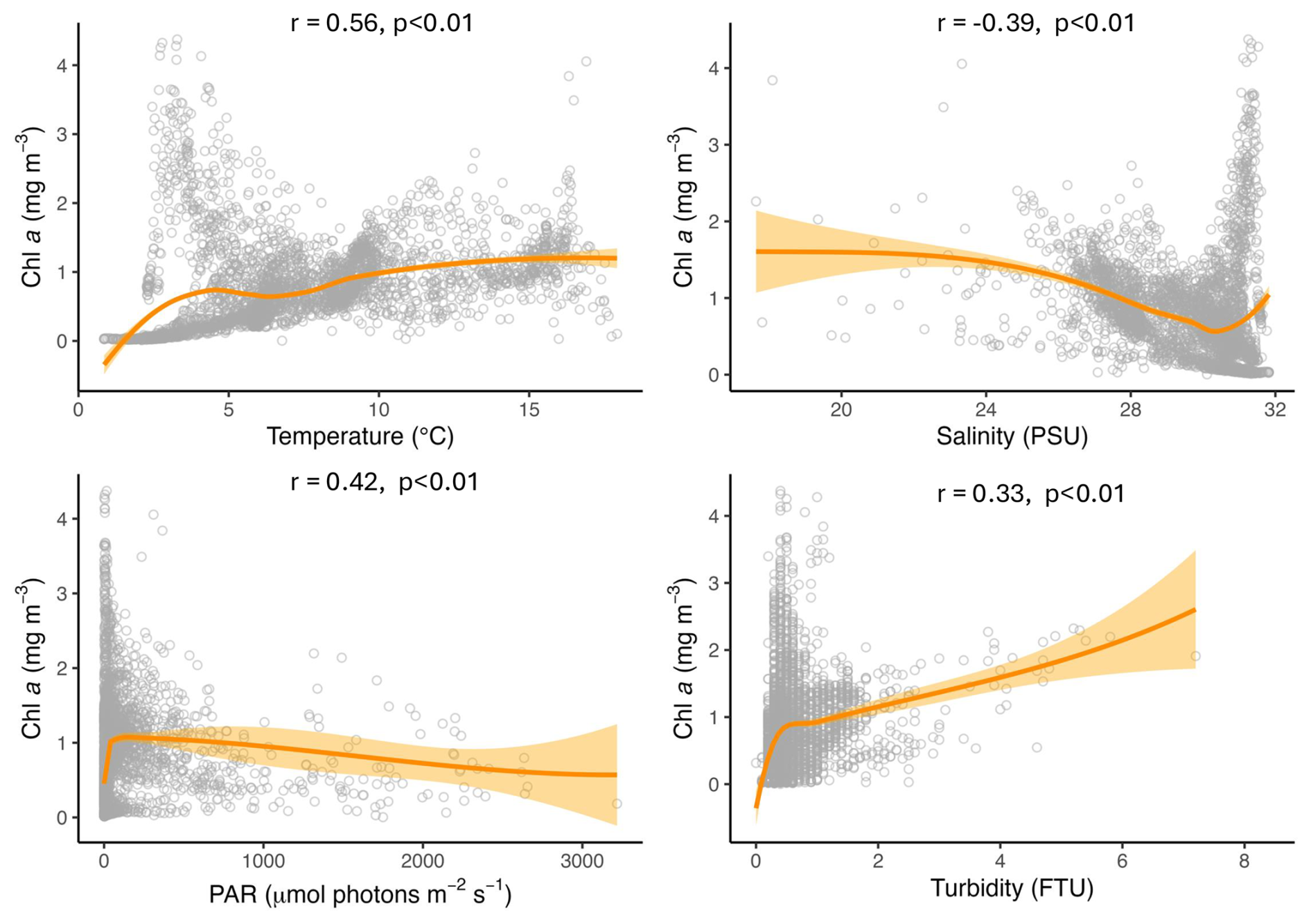
Figure 8 Scatter plots showing the relationships between Chl a and temperature, salinity, PAR and turbidity across the transect. The orange line represents the LOESS curve with 95 % confidence interval (shaded area). The Spearman correlation (r) and its p value are also indicated.

4 Discussion

This study shows that the water column properties near the coast of the Sept-Îles area undergo changes during the ice-free season, shifting from cold, well-mixed waters in spring to pronounced stratification in summer, particularly in July and August. The thermal stratification gradually deepens in September and disappears by October, with waters mixing and returning to more uniform conditions in autumn. Our study also highlights seasonal variability in Chl a, with high concentrations observed below the thermocline in July and fewer peaks observed at the surface in September near river sites. Most of the Chl a peaks recorded through the season occurred in July, at lower temperatures and higher salinity. Based on this dataset gathered in 2022, the Sept-Îles area shows the typical seasonal variability of a temperate coastal environment (Cloern, 1991; Leppärante and Myrberg, 2009; Galbraith et al., 2024b; Lim et al., 2025). In the Gulf of St. Lawrence, phytoplankton blooms are generally observed in spring followed by a secondary bloom in autumn (Galbraith et al., 2024b). However, this pattern differs in the present study, since the main bloom was observed during summer, perhaps due to the fact that we did not sample at the end of April, when the spring bloom might have occurred. Previous studies on pigments and phytoplankton assemblages carried out in the BSI, reported similar results; a seasonal variability in primary production with peaks of Chl a occurring in April, June and September (Lefebvre, 2023; Araújo et al., 2022). This seasonal dynamic may already be influenced by current climate change. The Gulf of St. Lawrence, historically covered with sea ice until mid-March, has experienced 4 nearly ice-free winters since 2010 (Galbraith et al., 2024a). Changes in sea ice cover are also occurring in the BSI, where sea ice has been disappearing sooner than usual over the past few years, and its formation and movements are becoming unpredictable (Allard, 2024). According to Allard (2024), these changes during the winter season could impact primary productivity in the BSI. Sea ice changes can affect spring bloom timing and the composition of phytoplankton species, thus impacting the whole food web (Pärn et al., 2022; Castagno et al., 2023; Nielsen et al., 2024). A possible small trend towards an earlier and more intense spring bloom was observed by Laliberté and Larouche (2023) between 1998 and 2019 in the St. Lawrence Estuary and Gulf, and they associated this trend with the decreasing length of the sea ice season.

In May, temperature and salinity were stable across the water column, but a warmer, brackish surface layer started to develop, marking the beginning of thermocline formation. This layer is heated by the sun during summer, while freshwater continues to flow from rivers into the coastal area. As observed in our study, lower salinity was mostly found at localized places in proximity to estuaries, e.g., sites 29, 30 and 31, near the Moisie River in May and sites 11 and 12 next to the Brochu and Ste-Marguerite rivers in September, all coinciding with peak river discharge (Carrière et al., 2018a). The influx of freshwater also increased turbidity at river-influenced sites such as Site 11, next to Brochu River. The well-mixed water column in May, and June, could also be linked to wind. Wind speeds recorded during these two months were stronger than those observed in the other months (Table A1). Phytoplankton abundance remained minimal with fluorescence averaging 0.097 mg m⁻³. Lefebvre (2023) identified April and May as the most productive months in the BSI during summer 2017, an observation that does not align with our study, as all concentrations of fluorescence were below 1 mg m⁻³ in May 2022. According to Araújo et al. (2022) the spring bloom in the BSI in 2017 occurred in April to early May before the spring freshet, when diatoms were the main phytoplankton group. Our first sampling was conducted at the end of May, between the 24 and the 26 May, probably after the spring bloom. Furthermore, Araújo et al. (2022) and Lefebvre (2023) using the same dataset, carried out their sampling mostly at the surface, whereas we measured the whole water column, which could be another reason explaining the differences in our results.

In mid-June, the water column was generally warmer, except at deeper sites such as Site 31, which reached 52 m in depth. A deeper thermocline layer marked the limit between the warmer mixed layer and the colder, saltier deep waters. In June, thermocline and pycnocline depths were not always aligned and differed among zones. In Zone 2, the pycnocline occurred above the thermocline, whereas in Zone 3 the pycnocline was deeper, indicating that density stratification was mostly influenced by salinity in June. As for variation in Chl a, only a few sites (17, 18 and 19, all located in the BSI in front of Anse à Brochu) recorded a Chl a concentration exceeding 2 mg m⁻³. These sites also recorded the highest turbidity and still showed highest concentrations of Chl a along the transect. Usually, turbidity limits phytoplankton biomass by reducing light penetration (Cloern, 1987; May et al., 2003). However, given the shallow depth at these sites, particularly sites 17 (2 m) and 18 (6 m), it is possible that the sampling process, including boat anchoring and the use of the CTD instrument, contributed to sediment resuspension. It could have brought particles from the bottom layer to the surface and affected turbidity measurements. Wind, tides and waves can also have an influence at these shallow sites. Furthermore, the presence of phytoplankton or other organisms also affects turbidity measurements. However, such high turbidity levels were only observed in June. Another explanation could be the location of Anse à Brochu that is at proximity to industrial activities and private docks. This area is also next to a discharge point for stormwater and municipal sewage discharge (Carrière et al., 2018b). Given the importance of these industries and the traffic of vessels, it is possible that these aspects contributed to sediment resuspension, influencing Chl a concentration. This also aligns with Lefebvre (2023), who observed a peak of Chl a (>5 mg m⁻³) at this same location in June 2017, associated with a dinoflagellate bloom. Furthermore, Liu et al. (2018), found that in high turbidity environments, temperature had a greater impact than light intensity on the timing of blooms. This could potentially be the case in our study.

Thermal stratification appears to play an important role in structuring plankton communities. Lim et al. (2025) found that plankton diversity and richness in coastal waters of southern Korea were lowest in July, coinciding with strong thermocline formation, whereas diversity peaked in September when stratification weakened. Additionally, their results indicated that plankton abundances below the thermocline were significantly lower than in the upper layer. In contrast, our study found that the highest Chl a concentrations were in July and were predominantly located below the thermocline. As seen in Figs. 2 and 7, the highest concentration of Chl a was deeper in the water column and at low to moderate PAR, but where nutrients are sufficient for growth. However, nutrients were not measured in the present study. Furthermore, halocline and pycnocline depths remained closely aligned throughout the study period, indicating that salinity was the main control on density stratification in this system. During summer months, however, the thermocline extended deeper than both the halocline and pycnocline. This coincided with the subsurface Chl a maxima observed in July, which occurred below the thermocline and at depths exceeding the pycnocline. These maxima therefore appear to align more closely with the lower boundary of the thermocline rather than the pycnocline, suggesting that thermal stratification may better explain the vertical distribution of Chl a in the studied region than density stratification alone. In oceanic environments, Chl a concentration varies dynamically and often shows maximum values in the subsurface of the layer rather than at the surface (Yasunaka et al., 2022). In the East China Sea, similar results were found, where the highest Chl a concentrations were recorded at the bottom of the thermocline. This was associated with a change in nutrient concentrations, where phytoplankton had access to a greater supply of nutrients at depth (Wu et al., 2002). Given that nutrient availability is a key driver for phytoplankton in the water column (Browning and Moore, 2023; Wei and Zhao, 2025), the higher Chl a concentrations below the thermocline in our study could potentially be explained by nutrient accumulation in deeper layers rather than light availability. However, some studies still find high Chl a concentrations even when nutrients are depleted, as observed in the Baltic Sea (Stramska and Jakacki, 2024). This suggests that other processes, such as upwelling events and currents, may also influence Chl a distribution. For example, at some locations of our transect, environmental conditions changed in July compared to June. Site 34, for example, recorded a decline in temperature from 10.2 to 5.63 °C during this time. Likewise, Site 31 (near Moisie River) exhibited higher salinity in July than in June. Furthermore, most peaks of Chl a occurred at lower temperatures and high salinity (Fig. 7), suggesting potential upwelling events. Several areas in the Gulf of St. Lawrence, including the north shore of the Gulf, are known to be in upwelling areas (Bourque and Kelley, 1995; Doyon and Ingram, 2000). These events are often associated with high Chl a concentrations, as they bring cold, nutrient-rich deep waters to the surface (Roegner et al., 2011; Diez-Minguito and de Swart, 2020). A 22 year time series by Laliberté and Larouche (2023) showed a strong positive trend in Chl a along the Gulf's North Shore, that they associated with stronger upwelling events generated by favorable winds. Modeling studies suggested that increased wind speeds may enhance upwellings along the north coast of the Gulf, potentially offsetting surface warming (Long et al., 2016). Although no long-term data currently exists for our specific study area, the elevated wind speeds observed in July may have facilitated vertical mixing and nutrient transport, contributing to the observed Chl a maxima. The vertical concentration of Chl a below the thermocline in July may also partly explain why fluorescence was a weak predictor of light attenuation compared to turbidity along the transect. Since Kd integrates attenuation throughout the entire water column, Chl a peaks that are lower in the water column, would contribute less to overall light attenuation than particles from the surface. Unlike findings in some estuarine environments where phytoplankton and suspended particulate matter both contributed to light attenuation (Lund-Hansen, 2004), turbidity was the dominant driver in the Sept-Îles area. This suggests that inputs from rivers and activities in the BSI played a greater role than phytoplankton biomass in controlling light availability. This is consistent with the higher light attenuation observed at river-influenced and urban sites, particularly within the BSI, compared to the eastern sites which showed lower attenuation reflecting a more pristine environment.

By August, we observed that the highest Chl a concentrations (>2 mg m⁻³) had shifted above the thermocline. This shift may have been driven by surface heating, with observed temperatures increasing during summer between July and September. This deepens the thermocline over time and alters vertical distribution patterns, contributing to variability in phytoplankton abundance. The surface layer in August also showed a lower salinity above the thermocline, reflecting river runoff and the beginning of the secondary summer bloom observed here and in earlier studies (Carrière et al., 2018a; Lefebvre, 2023).

September brought the warmest water temperatures of the year, likely due to heat accumulation over the summer months. Air temperature reached its peak between mid-July and mid-August (Table A1), contributing to the deepening of the thermocline during this period. Despite differences between our spring results and those of Araújo et al. (2022) and Lefebvre (2023) in the BSI, we found similar results for September. Fluorescence showed surface peaks at sites 7, 12 and 13, located outside the BSI. Although these peaks were at different locations than those sampled by Lefebvre (2023), who focused on sites within the BSI, they still demonstrate that there is observable phytoplankton activity in early autumn. The location of these peaks also suggests environmental and anthropic influences. Site 7 is in proximity to the industrial zone of Port-Cartier, close to the outflow of several streams, and sites 12 and 13 are located near the Brochu River. The latter is of ecological significance as a highly productive salt marsh ecosystem is found at its mouth (Bourque and Malouin, 2009). These sites also exhibited freshwater influence since they represented the area along the transect with the lowest surface salinity, especially in September. However, turbidity at these sites remained relatively low, averaging only 1 FTU. This could indicate a peak in river discharge influencing phytoplankton dynamics through nutrient inputs, that were not measured for this study. A study in a similar environment, a Chinese bay under anthropogenic effects, found that nutrients via river inputs had the greatest influence on Chl a concentrations (Wang et al., 2024).

Finally, the water column returned to well-mixed conditions in October, with fluorescence declining, and the complete disappearance of the thermocline, with the exception of Site 30 that still showed a residual deep thermocline. In the first meter at surface along the transect, freshwater influence was still noticeable but did not impact the rest of the water column. October recorded higher turbidity at certain sites, mostly located within the BSI. The BSI has a counterclockwise circulation, which tends to concentrate freshwater discharges from the four rivers in the Pointe-Noire area (Shaw et al., 2022; Paquette et al., 2018). This circulation pattern likely explains the elevated turbidity in this area in October, while also accounting for the absence of a freshwater signal despite the numerous streams and rivers flowing into the BSI.

5 Data availability

The complete CTD data used in this study are available in the Borealis database: https://doi.org/10.5683/SP3/ALRWON (Arseneault and Saulnier-Talbot, 2025a).

6 Conclusion

This study of water column dynamics during the ice-free season in a subarctic coastal environment documented seasonal variability of key ecological parameters including temperature, salinity and Chl a. The region of Sept-Îles has a highly dynamic coastal ecosystem where environmental conditions fluctuate daily. Although the typical spring bloom was not recorded, likely due to sampling starting after its peak, seasonal trends in thermocline formation and Chl a distribution were observed throughout the ice-free season. This clear seasonal variability has also been observed in similar environments such as the South of the Baltic Sea, where a thermocline forms in the beginning of May and starts to deepen in September due to autumn cooling (Leppäranta and Myrberg, 2009). However, due to the dynamic nature of the study area and its shallow depths, thermoclines and observed water column trends can change within a day. For instance, Carrière et al. (2018a), could not detect a thermocline in the BSI in summer 2016, potentially due to sampling dates that may not have aligned with peak stratification periods. Furthermore, lowest salinity values occurred during spring and early fall, coinciding with peak river discharge. Paquette et al. (2018) explained that these local freshwater layers can persist from a few hours to a few days in calm conditions. The results of our study depict the near-shore water columns at specific dates, as sampling was carried out only once per month. This shows how phytoplankton biomass variability is high in dynamic environments with complex physical parameters interactions, as previously suggested in similar studies (e.g. May et al., 2003).

Incorporating nutrient and oxygen monitoring would be essential to further improve our understanding of the mechanisms driving Chl a variability in the water column of this region and detecting potential upwelling events or eutrophication. Sept-Îles represents a high-use coastal ecosystem, under the influence of climatic and anthropogenic pressures, highlighting the importance of long-term and regular monitoring to detect environmental changes. Climate-related impacts such as changes in sea ice cover, wind regimes and the intensity of upwelling events may influence primary productivity. Therefore, regular monitoring of the water column, especially Chl a, is crucial to detect trends in phytoplankton dynamics and to assess broader ecological impacts of environmental change. This study complements prior work and will be useful for future studies and environmental monitoring in the region.

Appendix A

Table A1 Meteorological data for sampling days (in bold) and the previous week. Data retrieved from the Government of Canada at the Sept-Îles Station (Government of Canada, 2025). Temperatures are air temperature (no water temperature data is available).

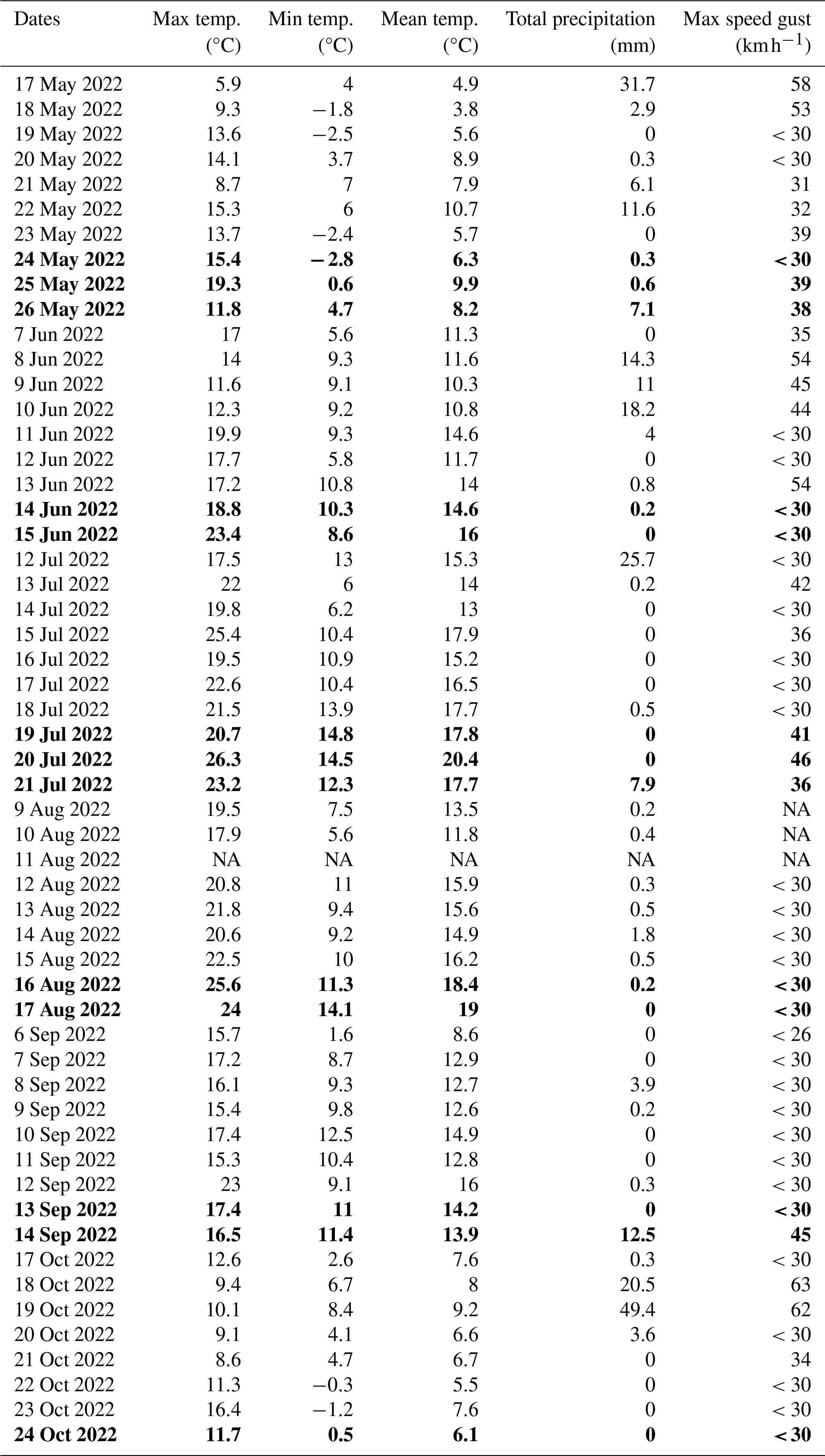
Table A2 Mean, standard deviation and range of temperature, salinity, turbidity, fluorescence, and PAR in the surface water of the three site zones for each month of sampling.

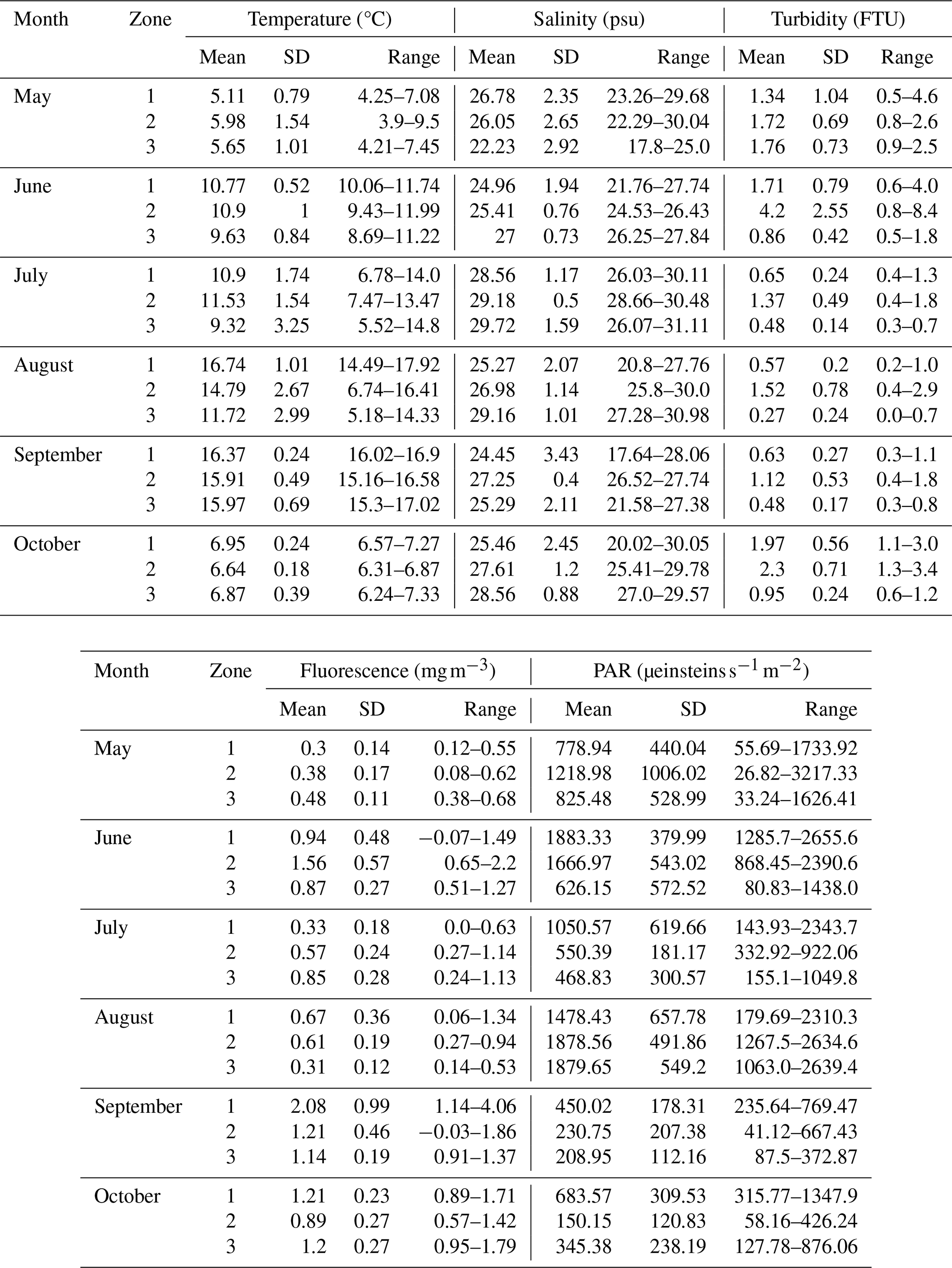
Table A3 Mean (± SD) depth of the thermocline, halocline, pycnocline, euphotic zone, and subsurface fluorescence maxima (Sub. fluor. max.), and mean stratification index, by the three site zones and sampling month.

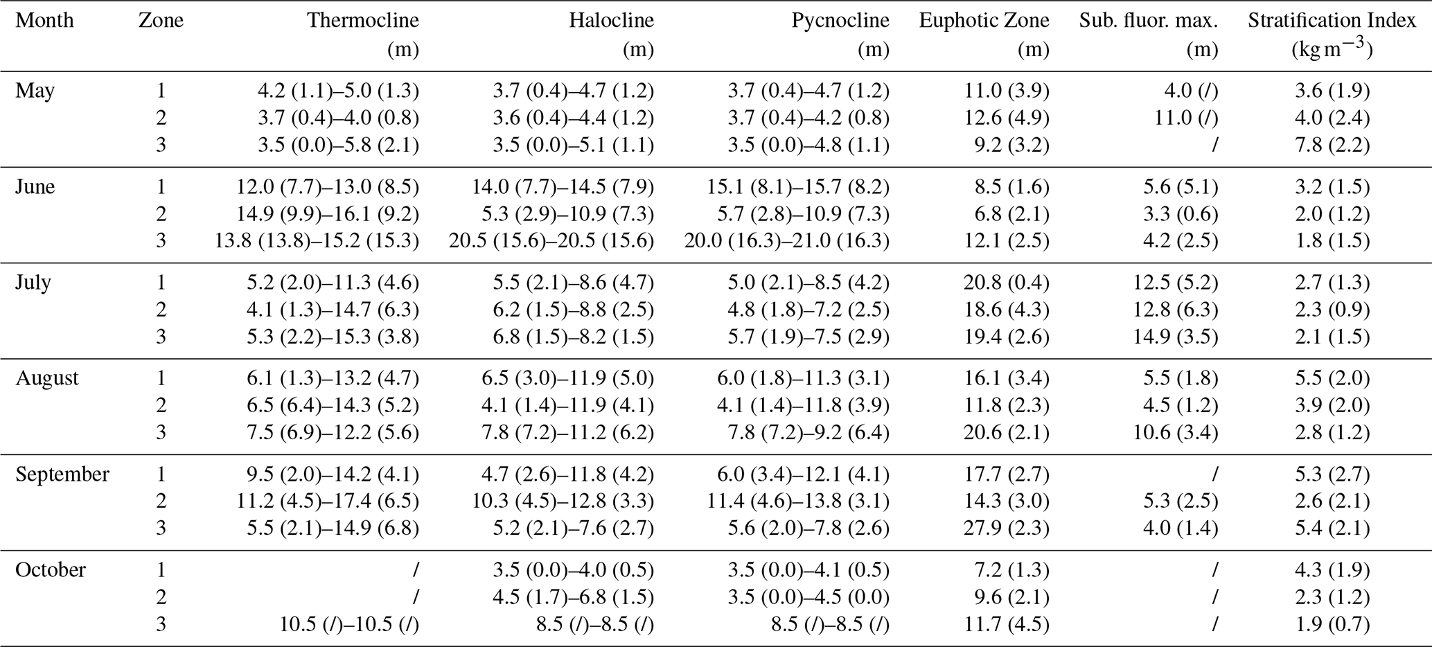
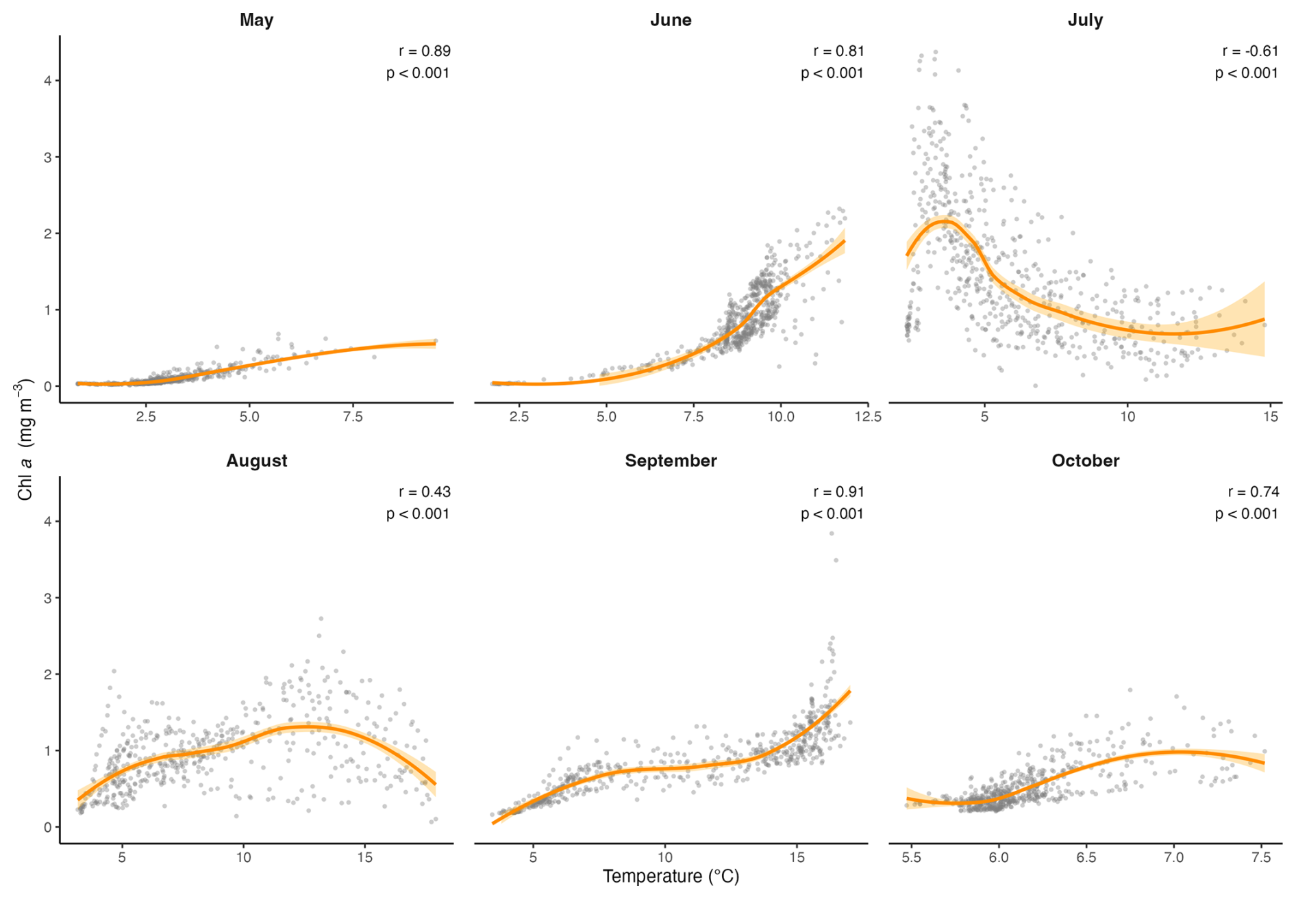
Figure A1 Scatter plots showing the monthly relationships between Chl a and temperature, across the transect. The orange line represents the LOESS curve with 95 % confidence interval (shaded area). The Spearman correlation (r) and its p value are also indicated.

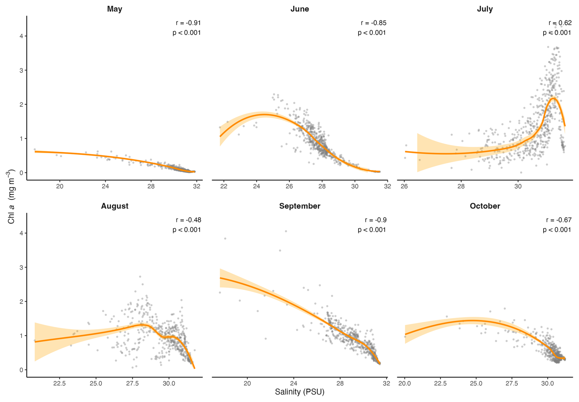
Figure A2 Scatter plots showing the monthly relationships between Chl a and salinity, across the transect. The orange line represents the LOESS curve with 95 % confidence interval (shaded area). The Spearman correlation (r) and its p value are also indicated.

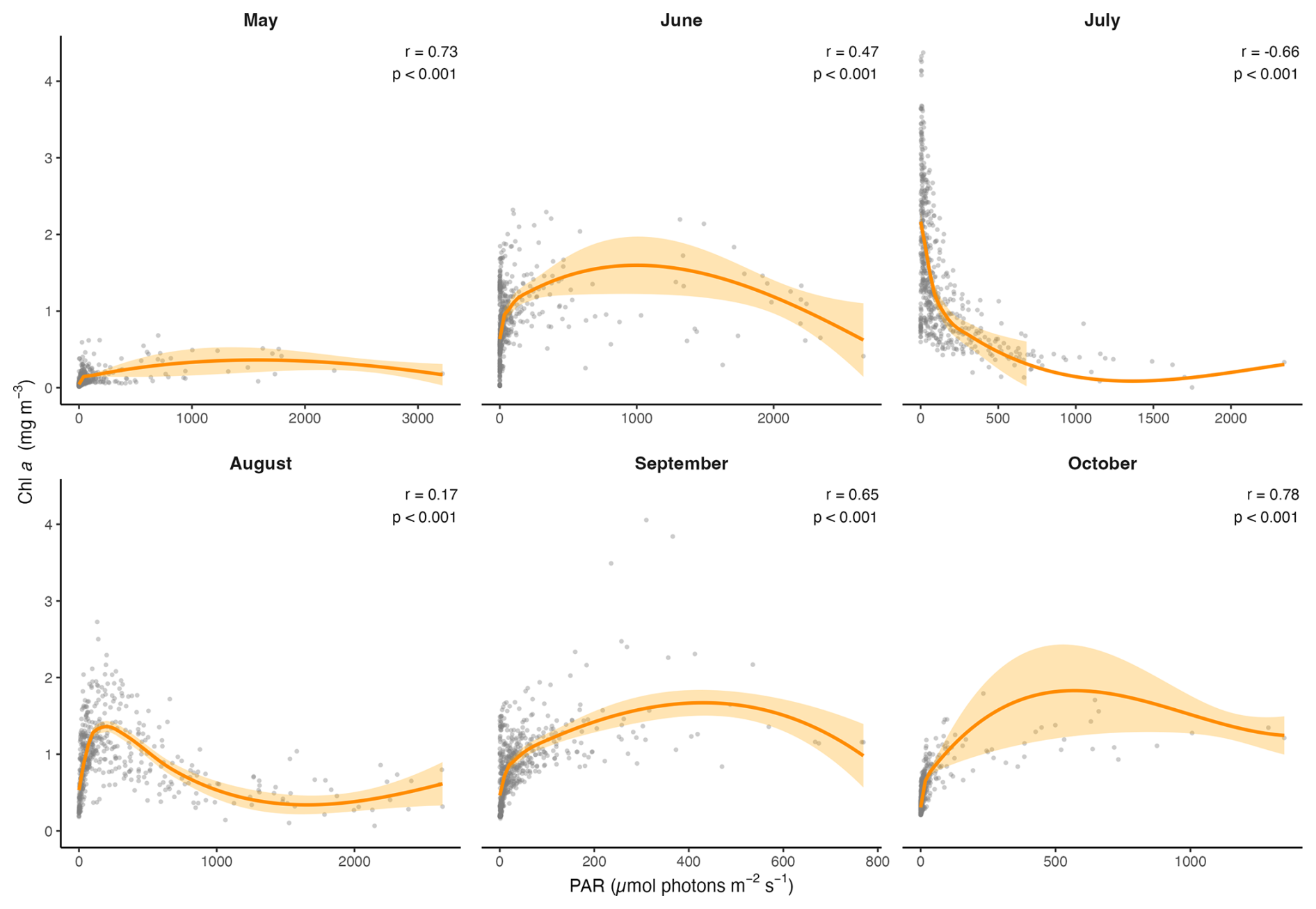
Figure A3 Scatter plots showing the monthly relationships between Chl a and PAR, across the transect. The orange line represents the LOESS curve with 95 % confidence interval (shaded area). The Spearman correlation (r) and its p value are also indicated.

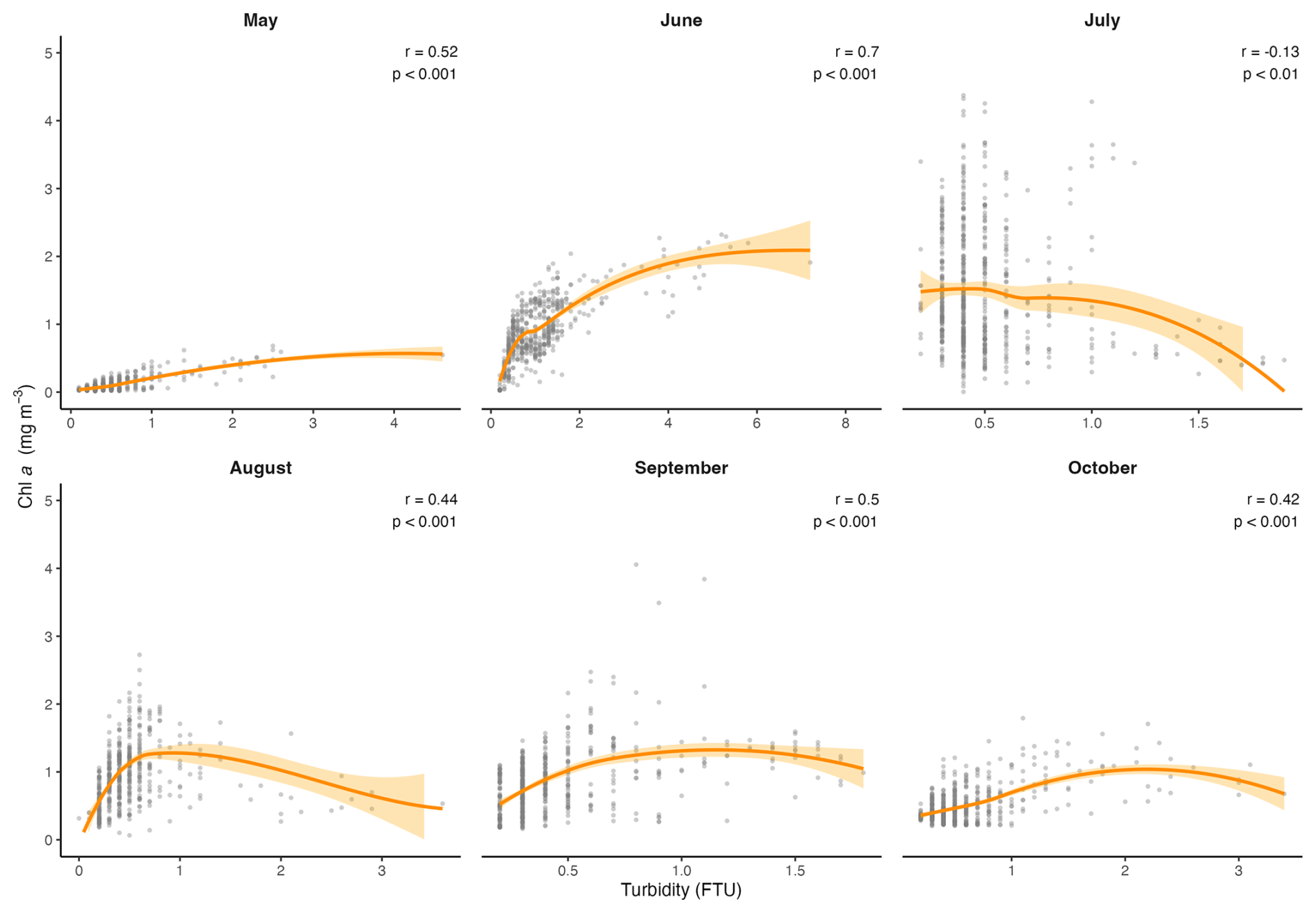
Figure A4 Scatter plots showing the monthly relationships between Chl a and turbidity, across the transect. The orange line represents the LOESS curve with 95 % confidence interval (shaded area). The Spearman correlation (r) and its p value are also indicated.