CAMELS-FI: hydrometeorological time series and landscape properties for 320 catchments in Finland

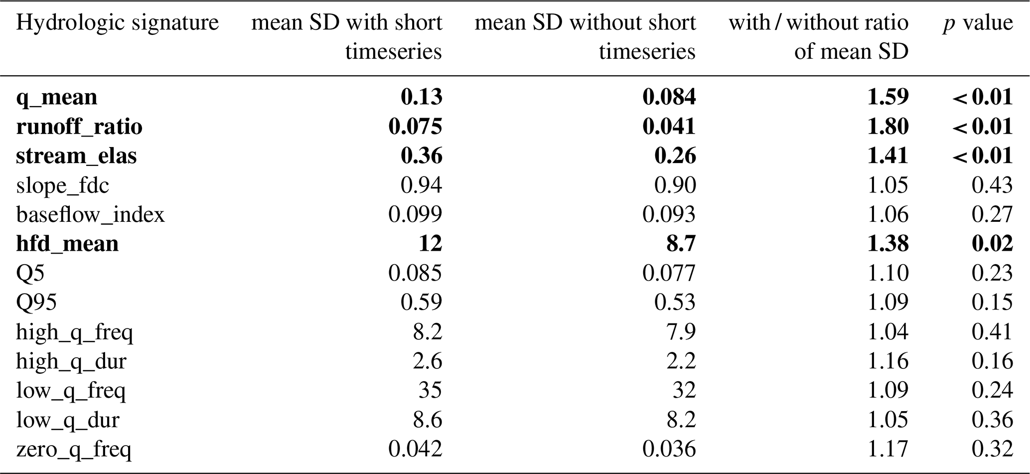
Comprehensive, large-sample hydrological datasets, such as CAMELS (Catchment Attributes and MEteorology for Large-sample Studies), have provided the basis for advances in many aspects of hydrological research in recent years. They can be utilised for several purposes, such as training or calibrating hydrological models, comparisons between regions dominated by different types of hydrological processes and testing of general validity of hydrological theories. The value of these datasets is in combining a multitude of data sources into one easily accessible and usable, harmonised high-quality package. We present CAMELS-FI, an extensive dataset for 320 catchments in Finland. It combines hydrological and meteorological time series with biophysical and human influence catchment attributes in a format that enables comparisons between catchments within the dataset but also between earlier CAMELS datasets. CAMELS-FI includes a diverse set of catchments with human influence varying from near natural to heavily regulated. CAMELS-FI is available at https://doi.org/10.5281/zenodo.15853357 (Seppä et al., 2025).

1 Introduction

One of the main goals of hydrology as a science is to understand and represent hydrological processes well enough to be able to simulate hydrological processes across the huge natural variations of hydrological settings, and multiple spatiotemporal scales (Gupta et al., 2014). Achieving this requires complementing detailed short-term investigations at a few locations with large-scale and long-term studies that help identifying general trends and patterns. These sorts of research approaches require large-scale discharge datasets, which have only become widely available in the past decade (e.g., do Nascimento et al., 2024; Turner et al., 2025). The general benefits of these datasets are manifold. Collection and proper quality control of large datasets with many variables is very time consuming, and using existing datasets helps reach results faster. Dedicated large sample hydrologic datasets are also typically well documented, citable, versioned and easy to bulk download. They follow the FAIR (findable, accessible, interoperable and reusable) principles (Wilkinson et al., 2016). Together these factors make it easy for researchers to use the data in a way that suits them. This has scientific benefits beyond individual researchers and studies. Since many researchers can use the same datasets, commensurability and repeatability of studies is enhanced, and new models can be benchmarked against existing ones without the need to implement and rerun all the previous models.

However, global or continental hydrologic datasets are often limited in many aspects. Firstly, global hydrology datasets are limited to global weather, soil, geology and land cover datasets, which often have relatively coarse resolution and might fail to take into account locally relevant conditions (Clerc-Schwarzenbach et al., 2024). Secondly, quality and time series length of discharge measurements vary wildly between different countries (Hasan et al., 2024). Thirdly, the number of stream gauges (subsequently referred to as gauges) in these datasets is often limited compared to the actual number of gauges. For example, the Global Runoff Data Center (GRDC) includes only 111 gauges from Finland, while the total count is over 650 current or historical gauges (Hydrologiarajapinta, 2026). Some global or continental datasets also directly provide just hydrologic signatures instead of daily or hourly discharge values (e.g., Chen et al., 2023; do Nascimento et al., 2024). This can hide issues with data quality, as well as create misleading results when indices developed for a specific hydroclimate are applied in other hydroclimate zones (McMillan et al., 2023).

Nationwide hydrological datasets aim to be useful for large-scale hydrology while avoiding many of the pitfalls of global datasets. National agencies of many countries produce and openly publish a lot of different high-quality environmental datasets that cover their country of origin, but do not typically extend beyond national borders. Thus, nationwide data allows for high-quality, consistent data and relatively large catchment counts at the same time. One of the most widespread national scale approaches is the CAMELS (Catchment Attributes and MEteorology for Large-sample Studies) datasets. They combine daily or hourly discharge measurements with catchment averaged daily meteorology and more slowly changing “static” attributes, such as topography and soil types. They also provide attributes and metadata in English, which expands the number of researchers that are able to understand and use the data, compared to the underlying datasets which are quite often only accessible in the language(s) of the particular country. Since the publication of the first CAMELS dataset for the continuous USA (retronymed CAMELS-US in this article to avoid confusion with the group of datasets; Addor et al., 2017; Newman et al., 2015), CAMELS datasets have expanded into a family of relatively commensurable datasets, covering portions of Americas, Asia, Europe and Oceania (for a full list at the time of writing this article, see Appendix C). However, each CAMELS is distinct in minor ways in the catchment selection and the variables it provides due to data availability, goals of the creators and differences in the dominant drivers of hydrological processes. For example, CAMELS-US contains three different sets of meteorological forcings (Newman et al., 2015), CAMELS-FR provides a multitude of morphometric attributes (Delaigue et al., 2025), and CAMELS-CH contains more information on glaciers than other CAMELS (Höge et al., 2023). There have also been efforts to develop and improve the datasets and introduce new types of data both to existing and new datasets. These include, but are not limited to the inclusion of hourly discharge (Coxon et al., 2026; Helgason and Nijssen, 2024; Tran et al., 2025), water quality (do Nascimento et al., 2025), groundwater (Coxon et al., 2026), expanding the set of catchments (Fowler et al., 2025), or including finer spatial divisions and structure in addition to full catchments (Helgason and Nijssen, 2024; Klingler et al., 2021; Knoben et al., 2025). To improve international comparisons, discharge data and catchments of some of the CAMELS datasets have also been combined with global meteorology, geophysical and human influence datasets to form part of a quasi-global dataset called Caravan (Kratzert et al., 2023). However, this has resulted in a degradation of meteorological time series quality, highlighting that CAMELS datasets can be optimal for applications where both relatively large sample sizes and high-quality data are required (Clerc-Schwarzenbach et al., 2024).

One of the most important outcomes of CAMELS datasets has been a breakthrough in deep learning rainfall-runoff modelling. Multiple studies have confirmed that training a long short-term memory (LSTM) network on large-sample data improves accuracy and robustness of discharge predictions compared to using data limited to one or a few catchments (Gauch et al., 2021; Kratzert et al., 2018, 2019b, 2024). Crucially, LSTM networks trained on CAMELS datasets have been consistently shown to outperform calibrated conceptual and distributed, process-based models in both gauged and ungauged settings (Kraft et al., 2025; Kratzert et al., 2019a). CAMELS datasets have also proved to be useful for other hydrological research tasks. Exploring effects of changes in the environment, such as of droughts or urbanization, to discharge at large scales has been a common application (Fowler et al., 2021a; Han et al., 2022). They have also been used for broad array of other tasks, among them robust calibration and testing of traditional lumped rainfall–runoff models (Bloomfield et al., 2021; Fowler et al., 2021b), analysing relationship of dominant hydrological processes to hydrologic signatures (McMillan et al., 2022) and scrutinising popular performance metrics in hydrology (Clark et al., 2021; Klotz et al., 2024). Although CAMELS are created for large-sample studies, they are also convenient data sources for single-catchment studies, since they cover a large portion of rivers of interest in their country, which saves considerable time otherwise used for gathering and preprocessing. This is attested by the number of studies that have chosen to select just one or two catchments from a CAMELS dataset (Aguilar et al., 2021; Knoben and Spieler, 2022; Robins et al., 2022).

Finland has a wide range of high-quality, openly available environmental datasets and long time series of discharge data. However, these datasets have not been synthesized earlier into one consistent catchment-oriented hydrometeorological dataset that covers most of Finland and is accessible from one location. To resolve this data gap, we present CAMELS-FI, combining daily discharge values from 320 rivers with daily meteorology and various slower changing static attributes.

Our first central objective has been consistency and high quality of data. To ensure consistency, the same source datasets have been used for all catchments. High quality has been ensured by selecting good quality source datasets, and performing various numerical and manual checks to minimize the chance of errors in the final result.

Our second central objective has been to create a dataset that is comprehensive, diverse and useful to as many catchment oriented applications in Finland as possible. Thus, we decided to be more inclusive than exclusive when creating the catchment selection criteria (see Sect. 2.1). Despite this, we had to make an exception with catchments for which large portions are located outside Finland, as their inclusion would have contradicted our aim for consistency. As a result of inclusivity, CAMELS-FI includes catchments of all regulation levels and time series of varying lengths. This means that CAMELS-FI is applicable for more tasks, but often requires the end user to further create a selection that is suitable to their task.

Additionally, we have strived to ensure compatibility with previous CAMELS to the highest possible extent. However, each CAMELS has something unique, and the way of structuring the data exhibits great variation, forcing us to choose suitable reference datasets. We decided to most closely follow CAMELS-CH (Höge et al., 2023) and CAMELS-GB (Coxon et al., 2020) for selecting most of the attributes and naming conventions, as they were relatively similar, and many of the used attributes were easily available from Finnish data sources. Hydrologic and climatic indices were calculated with code created for the CAMELS-US (https://github.com/naddor/camels, last access: 25 February 2026; Addor et al., 2017), following the example of CAMELS-GB. CAMELS-SE (Teutschbein, 2024) was followed for soil attributes, as Finland and Sweden share similar geomorphology. The file structures, file types, file names and directory structure of the data follow the convention of CAMELS-GB in order to facilitate easier integration of CAMELS-FI with existing software that interfaces with CAMELS data.

2 Catchments

2.1 Catchment selection

The Finnish Environment Institute (SYKE), hydropower companies and regional Centres for Economic Development, Transport and the Environment (ELY centres; they have since been replaced by Economic Development Centers, but were still active at the end of 2023, the cutoff date for data in CAMELS-FI, which is why we use the old organization name) maintain hundreds of hydrological gauges with long time series in Finland. The data are shared openly through SYKE's Hydrology API (Hydrologiarajapinta, 2026; https://rajapinnat.ymparisto.fi/api/Hydrologiarajapinta/1.0, last access: 13 May 2026).

The catchments included in CAMELS-FI were selected according to the following criteria:

1. The gauge must have had observations in 1995 or more recently. This is to ensure that most of the gauges have concurrent observations.

2. A minimum of five years (1826 d) of observations required between 1961 and 2023. We wanted to include shorter timeseries than many previous CAMELS datasets, because short time series can still be useful for various applications, such as examining individual events or training a hydrological model. It should be noted that short timeseries may not represent longer term conditions (Sect. 6.2). Thus, the end user has to select the required length of timeseries for their application.

3. To aim for consistency, catchments with major areas outside of Finland were excluded due to using national datasets. However, the borders of Finland with Russia and Norway approximately (but not exactly) follow the basin boundary in many places, leaving relatively small portions of catchments beyond the border. Therefore, we decided to include catchments with less than 5 % of the area beyond the Finnish border (n=27), according to SYKE's catchment delineation data (Valuma-aluejako, 2023). This criterion led to the deletion of some gauges at headwaters in Oulu and Kemi river basins, while including gauges further downstream.

4. Finnish waterway systems include a considerable number of lake and river bifurcations. Some of these are natural and caused by flat topography or large and labyrinthine lake systems shaped by uneven post-glacial rebound (Kuusisto, 1984; Tikkanen, 2002). Others are artificial for the purposes of flood regulation, reservoir filling or to enable boat or log traffic (Kuusisto, 1984). We decided to exclude most gauges that are located within a bifurcated part of a watercourse, since those gauges measure only parts of the total discharge of the catchment. Multiple pour points are also incompatible with the catchment delineation method used in this study (see Sect. 2.2). However, we made exceptions in cases, where:

   • a.

     The bifurcating branches are in close proximity, and both had discharge measurements. In those cases, we created a “virtual gauge” by adding the discharge values of the two gauges together and relocated the gauge just upstream or downstream of the bifurcation, depending on the measurement gauge location and watercourse geometry. Artificial structures are often, but not always involved in these situations. Virtual gauges can be identified by their id, which is in the format (xxxx-)xxxx-xxxx instead of the typical (x)xxx in normal gauges.

   • b.

     The effect of bifurcation is minor compared to the total measured discharge. In these cases, the gauge was left in place, and correct catchment delineation was ensured with methods described in Sect. 2.2. This led to some gauges immediately downstream of a bifurcation being excluded, but gauges further downstream being included. Most notable bifurcation system like this are lakes Lummene and Vesijako shared between Kokemäki and Kymi river catchments. We also decided to include the gauges that are part of the bifurcation system of Lokka and Porttipahta reservoirs, where almost all of the water from Lokka has been directed to Porttipahta and its outlet Kitinen since 1991, outside of the exceptional flood peaks in 1993, 2000 and 2010. Previously, the discharges were more evenly distributed between the reservoirs. We included the Kammonen, Luiro (gauge 1358) at the middle reach of Luiro as a “virtual gauge” 1352–1358, by removing the discharge from Lokka (gauge 1352) from the discharge values of the following day of the gauge 1358, and removed the catchment area upstream of dam of Lokka from the catchment of the gauge 1358. The offset of one day was determined from comparing the discharge peak timing of high discharge events at gauges 1358 and 1352 in 1993, 2000 and 2010.

In total, the selection criteria led to 320 gauges (Fig. 1). Gauges 1190 and 1191 were from exactly the same location, just separated temporally, and therefore we combined them together to form virtual gauge 1190–1191. Following the regional division of Korhonen and Kuusisto (2010), all hydrological regions of Finland are well represented, although the Vuoksi drainage basin (we define a basin as an area drained by a shared outlet to a sea) in south-eastern Finland has large portions missing due to many internal bifurcations and a large part of the catchment being on the Russian side. The catchments have large variations in the level of regulation, please consult the human influence attributes to select catchments for specific use cases (see Sect. 4.7).

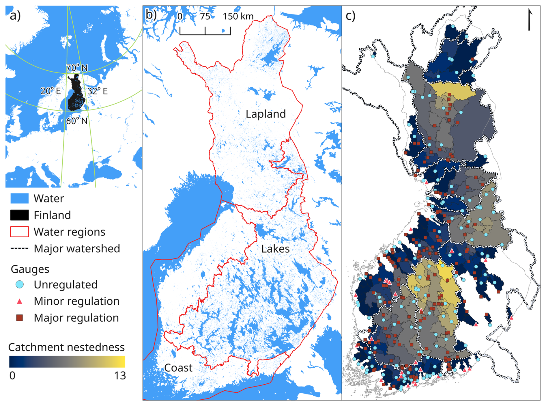
Figure 1 (a) Finland is located in northern Europe. (b) The main hydrological regions of Finland according to Korhonen and Kuusisto (2010). (c) CAMELS-FI includes catchments that are unregulated, minorly regulated and majorly regulated. The catchments are often nested. Smaller catchments are shown on top of larger ones.

2.2 Catchment boundaries

The catchments for the selected gauges were calculated with the Python bindings of WhiteboxTools (WB tools) (2.3.6), Geopandas (1.0.1) and Rasterio (1.4.3) using the Elevation model 10 m (DEM) of the National land survey of Finland (NLS) (den Bossche et al., 2024; Gillies et al., 2024; Lindsay, 2014; Elevation model 10 m, 2019). To ensure good quality catchment delineation, SYKE's river channel and level 3 basin division data were used as guiding features (Valuma-aluejako, 2023; Uomaverkosto, 2024). Due to the DEM only covering Finland, channel sections crossing the national border were removed, and in case of some minor bifurcations, the channel network was modified slightly. The known channels were virtually excavated one meter deeper than their surroundings, and the level 3 basin divisions were transformed into “walls”, except where they intersect with channels. Subsequently, the DEM was then breached and depressions filled with the “breach depression least cost” WB tool. Eight directional flow pointers were computed, streams were identified as places where at least 40 000 cells flow into that cell, and gauges were snapped to those streams. Some gauges had to be moved slightly so that they snapped to the correct location. After that, catchment boundaries were calculated for each gauge. All catchment boundaries were inspected individually by visualizing them alongside other catchments and all the other datasets used in catchment delineation, followed by a visual check for inconsistencies. The inspection always included both an overview of the whole catchment and a detailed, section-by-section examination of the entire border. Where inconsistencies were identified, additional virtual walls were added and the delineation procedure was repeated until a satisfactory result was achieved. Parts of the catchments crossing international borders were added manually by selecting and merging SYKE's level 4 basin divisions. The resulting catchments cover 73 % of Finland's total land area, and vary in size from 7 to 50 672 km² (median 762 km²).

2.3 Gauge and catchment metadata

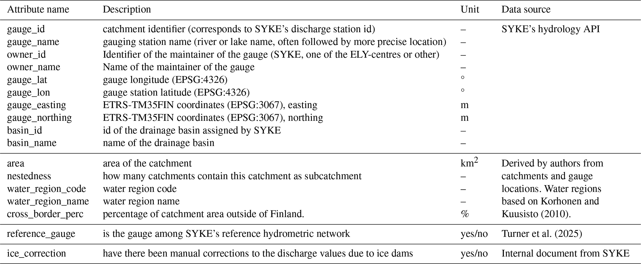
Diverse metadata attributes of the gauge and catchment are presented to support use (Table 1). Gauge location, gauge name and basin name were downloaded from SYKE's hydrology API. Nestedness, meaning the number of larger catchments in CAMELS-FI that the catchment is part of, the catchment area and the percentage of catchment outside of Finland were calculated for all catchments. The maximum nestedness is 13, and there are 77 catchments with nestedness of zero from 55 basins. Additionally, the hydrologic region of the catchment is also provided (Lapland, Lakes or Coast, after Korhonen and Kuusisto, 2010, Fig. 1b).

Table 1 Summary of gauge and catchment metadata in CAMELS-FI.

3 Hydrometeorological time series

3.1 Hydrologic time series

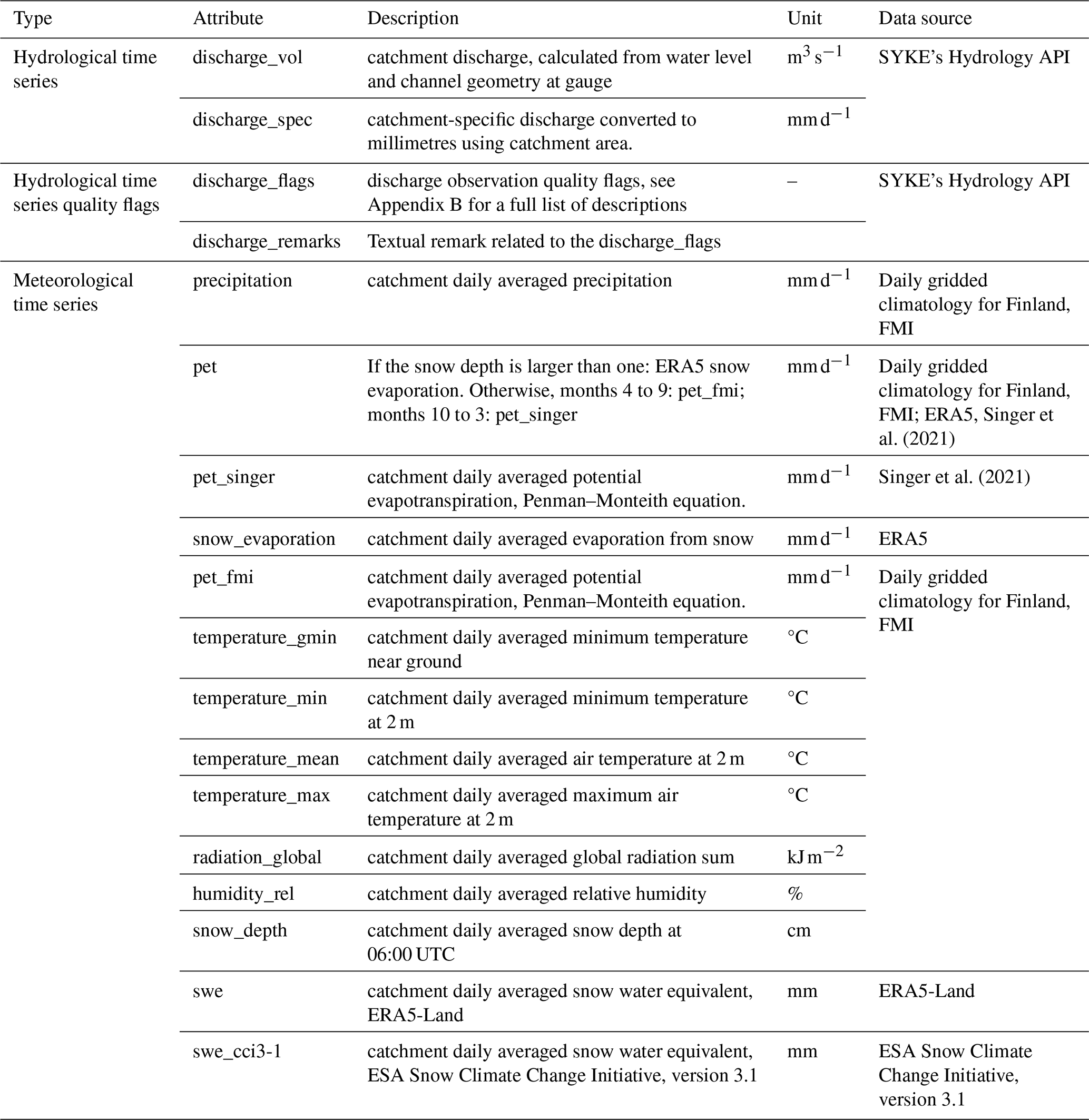
Daily volumetric discharge (Q, m³ s⁻¹) for 1961 to 2023 was downloaded from SYKE's hydrology API, and specific discharge (q, mm d⁻¹) was calculated based on catchment areas (Table 2). When it is not necessary to separate the two meanings, we use the term discharge without other specifiers. Volumetric discharge is calculated from water level using daily average water level and a rating curve, except for hydropower plants, for which the discharge values are provided directly by the operators. Rating curves are based on direct discharge measurements with mechanical current meters before 1990s and mainly with acoustic doppler current profilers (ADCP) after that.

Table 2 Summary of time series variables in CAMELS-FI.

Water levels have been measured continuously since the 1960s. Initially, observations were made using automatic limnographs equipped with wells connected to the main river channel or lake via pipes. In the 1960s, daily values were read manually from the limnograph each morning at 08:00 LT. From the early 1970s onward, daily mean water levels were calculated from the limnograph records and stored in a database. Measurement processes became digitalized from 1984 onwards up to the early 2000s, when automated systems using pressure sensors were introduced. During this period, daily average water levels were derived from hourly measurements.

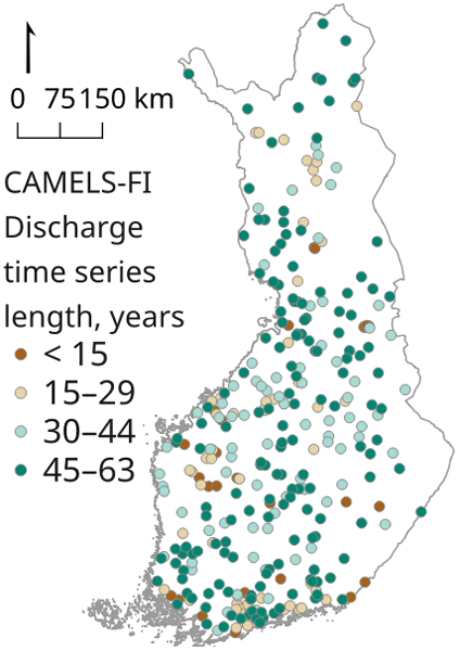
The length of the provided hydrological observation series varies from 5 to 63 years, with a median of 45 years and three quarters of the gauges have had observations for 30 years or more (Fig. 2). Each discharge observation has also a corresponding quality flag, with most common flags being normal observations (n=4 669 213, 91.4 %) and ice correction related discharge reductions (n=393 023, 7.7 %), while the rest indicate varying types of quality issues or corrections (n=44 226, 0.9 %). It should be noted that for virtual gauges, the quality flags of all contributing gauges are provided. For a full list of quality flag classes see Appendix B. Textual remarks related to small amount of the flags (n=13 282, 0.26 %), mostly from class “other” are also provided. The original remarks were in Finnish and were translated manually to English by the authors.

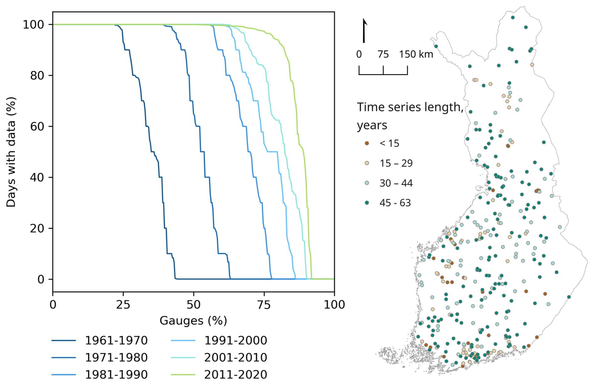
Figure 2 Time series length of hydrologic observations in CAMELS-FI. The number of gauges has increased gradually over the years, but some have also been decommissioned.

The 17 catchments that are part of SYKE's hydrological reference network and the global ROBIN (Reference Observatory of Basins for International hydrological climate change detection) initiative are indicated in metadata attributes (Turner et al., 2025). SYKE has put extra effort into ensuring that these gauges have very high-quality observations, and they are largely unaffected by human disturbances.

Supplementary daily discharge values are also provided for a few locations where water is pumped from one catchment to another. For these artificial bifurcation gauges, the only static attributes provided are the gauge metadata, and no catchment is provided. The locations are: Päijänne Water Tunnel (1092 and 1093); Paimio River to Aura River (1115); Lokka reservoir to Luiro River (1352) and Saimaa Canal to Rakkola River (3683). Overall, the effects for both source and recipient catchments are usually relatively minor, although the effect might be noticeable during low discharge. These artificial bifurcations are completely separated from the rest of the data and are not counted as catchments in CAMELS-FI.

3.2 Meteorologic time series

Daily meteorological attributes from 1961 to 2023 were derived for the catchments mainly from the Finnish Meteorological Institute's (FMI) 1 km×1 km gridded daily climatology of Finland (Aalto et al., 2016). The product has been created by applying Kriging with external predictors of lake and sea cover, elevation and relative altitude to FMI's observation network. It should be noted that minimum temperature near ground is missing from the original dataset from 16 October 2022 onwards, which is why it is also missing from CAMELS-FI. Potential evapotranspiration (PET) was only available for the months from April to September from 1981 onwards from FMI (Pirinen et al., 2022). Thus, we also include snow evaporation from ERA5 (Hersbach et al., 2020) and PET from Singer et al. (2021). Both FMI and Singer et al. approximate PET of well-watered grassland, Singer et al. with FAO Penman–Monteith equation (Allen, 1998), while FMI uses slightly modified version (Allen et al., 2006). In addition to providing the aforementioned data, we combined the data into one convenient PET attribute, which was also used for calculating climatic signatures (see Sect. 4.2). This was done by using snow evaporation when the snow depth of the catchment was over 1 cm, and filling the snow-free days with FMI PET if it was available; the remainder was completed by using Singer et al. (2021). We recommend using this combined PET, unless the end user has a specific reason to do otherwise, because it doesn't have temporal gaps, takes snow period into account in a reasonable way and provides the best available data for any month.

FMI does not include snow water equivalent (SWE) in their gridded product, only snow depth. However, as snowmelt typically causes most major high discharge events in Finland, we felt that including it was necessary. The SWE product in ERA5-Land has been benchmarked to perform overall better than other available products, so we chose it (Mudryk et al., 2025; Muñoz-Sabater et al., 2021). However, as there are many SWE products that have been benchmarked relatively similarly in non-mountainous regions, and there are some differences between the products, we decided to also include ESA's CCI3-1, which is available from the beginning of 1979, usually from October to May (Luojus et al., 2024). It is provided typically for every other day and has occasional gaps of two or three days, so gaps of less than three days were interpolated linearly to obtain daily values. See Sect. 6.3 for a brief comparison between the different snow products.

The catchments' daily values were extracted by calculating the areal average of the grid for each catchment, considering all pixels that touch the catchment to avoid problems with the smallest catchments for coarser resolution products. ERA5 and ERA5-Land offer hourly data, which were aggregated to daily values. The portions of catchments beyond Finnish borders were not included in the catchment borders used for calculations, as is the case for all static catchment attributes as well.

4 Catchment attributes

4.1 Hydrologic signatures

Hydrologic signatures were calculated from the daily specific discharge and precipitation data described in Sect. 3. Definition of the water year for Finland was obtained from Irannezhad et al. (2024), meaning that the water year starts on 1 September and ends on 31 August. Hydrologic signatures were calculated with available observations for the water years of the climatological standard period 1991–2020, except for a few gauges with less than five years of observations during the period, for which all available data were used. All those gauges had started measurements after 2015, excluding gauge 1353, which had a gap in observations between 1989 and 2020. Hydrologic signatures were calculated using code from https://github.com/naddor/camels (last access: 20 March 2025).

4.2 Climatic signatures

Climatic signatures of the catchments were calculated for water years 1991–2020 from daily precipitation, PET, and mean temperature, using code from (Addor, 2020; https://github.com/naddor/camels, last access: 20 March 2025). Additionally, mean temperature was calculated for all the catchments for the same period. We chose to use the combined PET that was described in Sect. 3.2 since it gave realistic yearly mean PET values for the full year.

4.3 Elevation

Topography descriptors were derived from the NLS's DEM, without hydrological preprocessing (Elevation model 10 m, 2019). For gauge elevation, the pixel touching the gauge location was used. Other elevation measures were derived by using all the pixels of the DEM that touch the catchment area. Please note that gauge elevation may differ significantly from the lowest elevation of the catchment due to deep open-pit mines inside the catchment, which is why both are provided.

4.4 Land cover

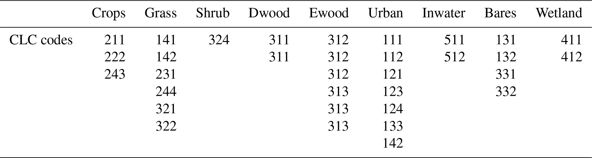
Land cover can change significantly on a decadal scale. Thus, instead of providing one value for each land cover class, we follow the example of CAMELS-CH (Höge et al., 2023), and provide values for all four CORINE Land Cover (CLC) products made for Finland, from the years 2000, 2006, 2012 and 2018 (Corine maanpeite 2000, 2002; Corine maanpeite 2006, 2008; Corine maanpeite 2012, 2014; Corine maanpeite 2018, 2020). Linearly interpolated yearly values for 2000–2018 are also provided per catchment. Unfortunately, we were unable to find earlier harmonized land cover time series datasets, so our land cover time series covers only the most recent decades. CLCs are produced nationally with harmonized criteria set by the European Environment Agency. We used the Finnish versions of CLCs, which have higher resolution and a smaller minimum feature area than the Europe-wide products. They have been created using existing datasets at SYKE combined with automated satellite image interpretation. We created a similar classification to CAMELS-CH and CAMELS-SE, which also used CLC as their land cover data. Each CLC edition has seen some small changes to the classes present, but in our opinion, these are largely inconsequential for hydrological tasks. Exact CLC classes used for each year are presented in Appendix A1.

4.5 Soil

Soil class areal portions were calculated for each class based on the Superficial deposits of Finland 1:200 000 (2018) soil classification map by the Geological Survey of Finland (GTK). It should be noted that the areal percentages of soil classes do not total 100, because water and built areas were excluded. These data are different from the soil information provided by most other CAMELS, since GTK classifies soils based on the dominant grain size, instead of providing weight portions of different grain sizes. However, Sweden has a similar soil classification system, and we decided to follow the soil classes present in CAMELS-SE (Teutschbein, 2024). It should be noted, that quaternary sediment deposits form mostly only a thin or, in some locations, a non-existent layer above bedrock, which is why bedrock is considered as a “soil” class. Descriptions of the exact soil classes used are presented in Appendix A2. In terms of groundwater, the most important landforms in Finland are eskers and terminal moraines (Fin. salpausselkä), which form the most important aquifers in Finland due to their high sand and gravel content (Katko et al., 2006). These landforms have a thin and long shape, meaning that they are poorly represented by coarse resolution datasets, which is why Global or Europe-wide soil datasets were considered unsuitable for Finland. Soil depth was averaged from the Superficial deposit thickness 1:1 000 000 product from GTK (Superficial deposit thickness 1:1 000 000, 2018).

4.6 Geologic

Rock type areal classes were calculated for each class based on the Bedrock of Finland 1:1 000 000 (Geological Survey of Finland, 2016) rock classification map by GTK. In Finland the bedrock is mostly crystalline and conducts water very poorly outside of fractures (Karro and Lahermo, 1999). Thus, the type of rock beneath the soil has only little influence on the discharge on the surface. Due to this, no national hydrolithological data exists for Finland, and hydrolithological attributes present in many previous CAMELS cannot be provided. Crack density could also be useful information for hydrology, but no good quality national dataset exists for Finland.

4.7 Human influence

CAMELS-FI contains catchments with vastly different levels of human influence, and multiple different attributes are provided to help dataset users decide which catchments suit their needs. Catchments are divided into three regulation classes based on regulation information from SYKE's Lake API (Järvirajapinta, 2025; https://rajapinnat.ymparisto.fi/api/jarvirajapinta/1.0, last access: 23 December 2025) and manual assessment of discharge plots. The classes are: No active regulation (n=131), Minor active regulation (n=26) and Major active regulation (n=163). Not actively regulated catchments may still have dams, but the dams only dampen natural variations slightly. They also include some catchments with a regulation permit that is either not used or its effects are nearly inconsequential for the discharge at the gauge, such as artificial permanent lowering of lake level before 1961. Minor active regulation includes catchments which have regulation that influences the discharge, but the end result is still relatively close to natural. Major active regulation includes the rest of the catchments where the discharge is strongly controlled, most commonly by a hydropower station with a reservoir. Gauge 3536 changed from majorly to minorly regulated in 2013, and was classified as minorly regulated. Reservoir capacity (difference between maximum and minimum) and count, as well as the count of other regulation types, are provided. We define a lake as a reservoir if the regulation permit has a known capacity; otherwise, it is deemed to be other regulation. Dam count is also provided based on NLS's Topographic Database (National Land Survey of Finland, 2024). It should be noted that the authors noticed some dams missing from the topographic database, so the given counts must be considered as approximate. The population count of each catchment, based on Statistics Finland's 1 km×1 km grid for 2023, is also included (Statistics Finland, 2024).

5 Regional variability and catchment properties

Hydrologic regions of Finland have differences that cause significant disparities in hydrological behaviour. Rainfall is greatest in the southern coast and high hills of the northern lake region, up to 750 mm yr⁻¹. The lowest rainfall occurs in northern Lapland, where rainfall can be as low as 470 mm yr⁻¹. However, mean temperature and mean PET are the highest in the southwest, and decrease towards the northeast, which results in Lapland and the northern lake region having the highest specific discharge (Figs. 3 and 5). The proportion of snow from rainfall follows a similar pattern.

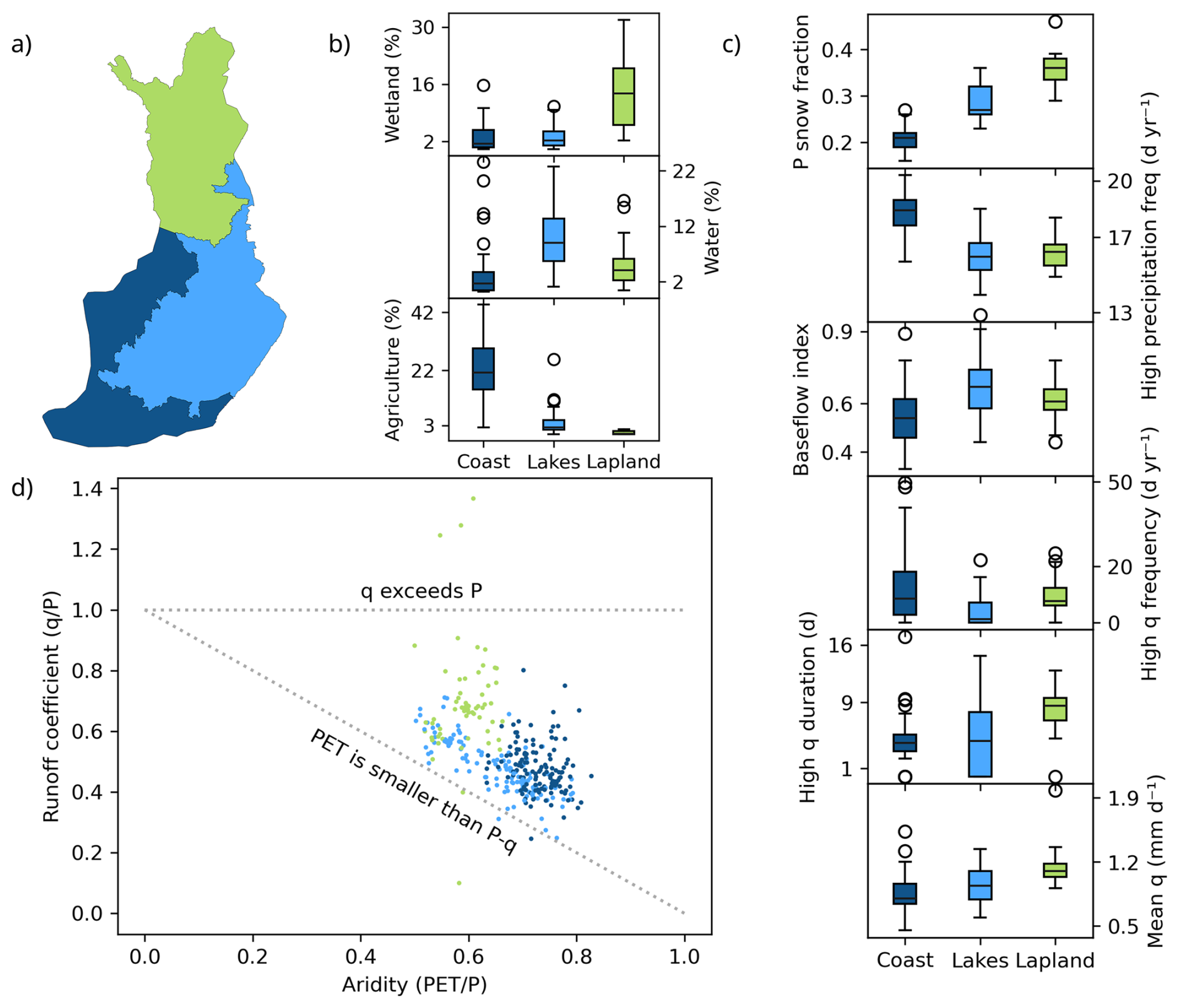
Figure 3 (a) Map of the colours used to mark hydrological regions for the rest of the figure. (b) Variation in land cover between regions. (c) Variation in climate and discharge regime between regions. Baseflow calculated with the methodology of Ladson et al. (2013). (d) Gauges plotted by runoff ratio and aridity. Inspiration for the figure from Fig. 2 of Coxon et al. (2020).

Flood patterns also differ between the regions. Lapland and the northern lakes typically have only one single flood event in the spring caused by snowmelt, while this is true for the coasts only in the coldest winters (Fig. 4). During milder winters, winter floods caused by (partial) snowmelt are common on the coasts, while northern parts may receive increased or normal snowfall due to warmer air being able to retain more water. Catchments with a high lake portion have dampened and elongated flood peaks and an overall higher baseflow index. Catchments on the coast are typically smaller or have fewer lakes than the other two regions, causing catchments there to react more rapidly to rainfall or snowmelt events. The coasts also receive, on average, more high precipitation events, which can cause local flooding, especially in cities.

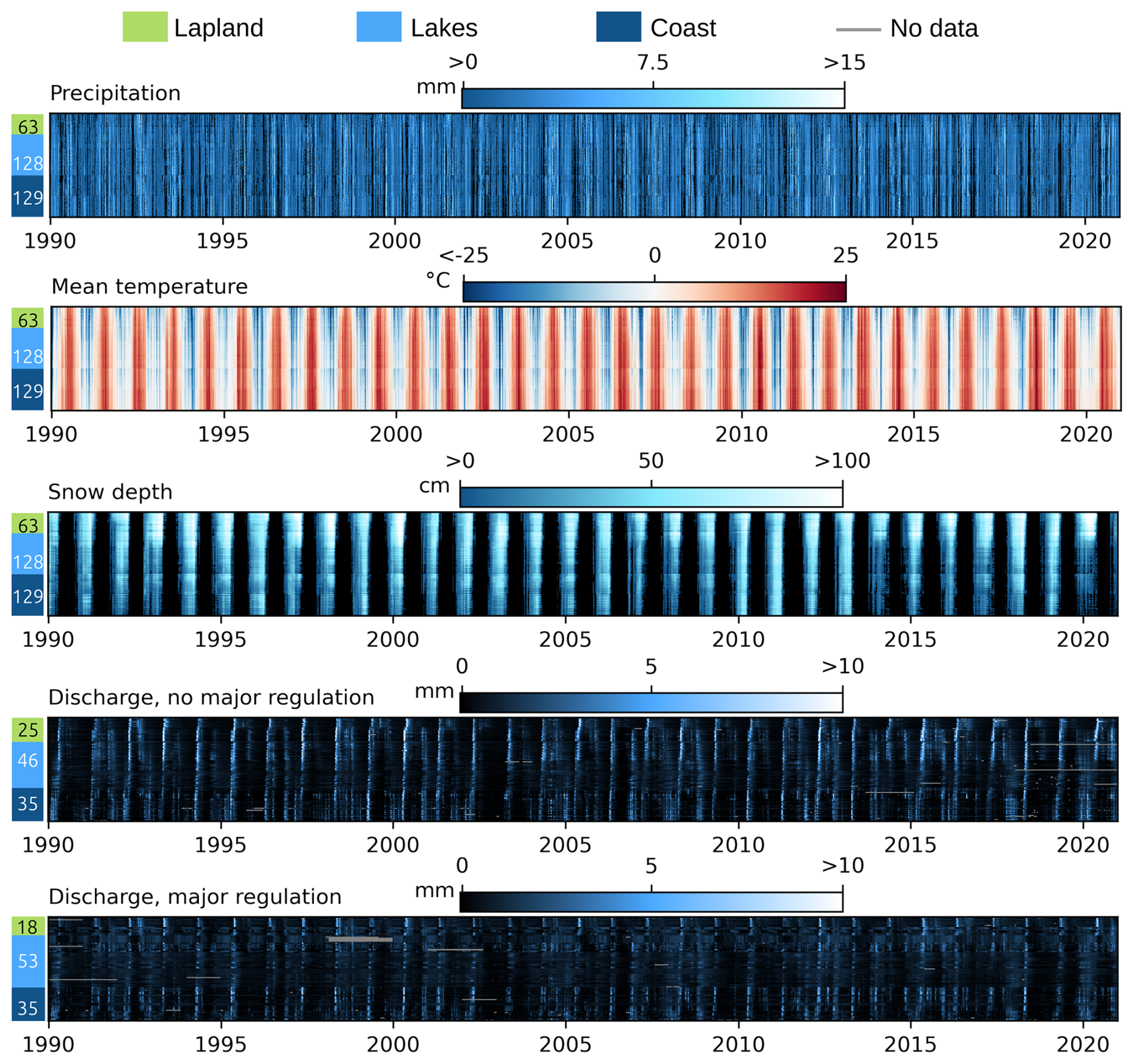
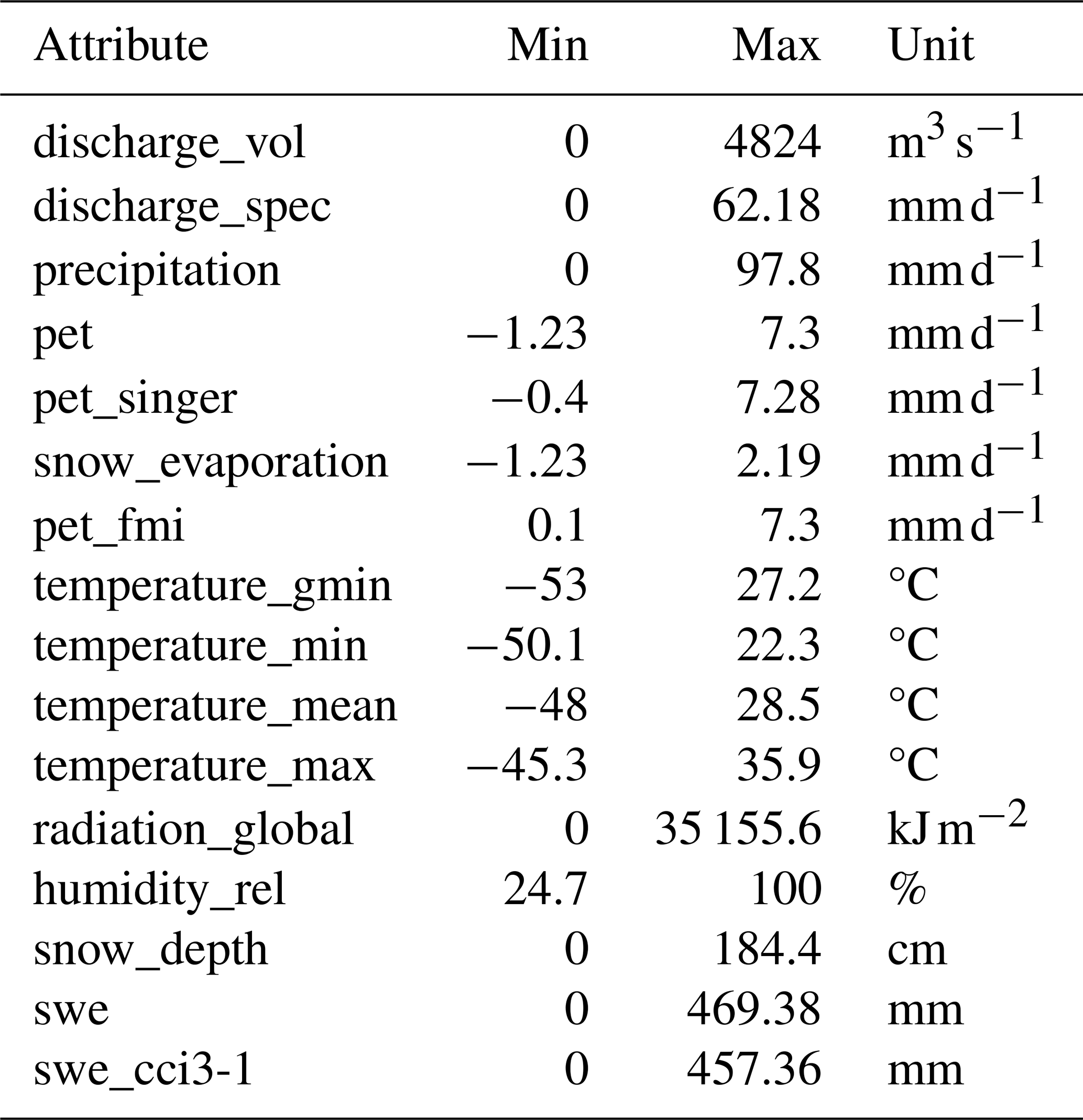
Figure 4 Key hydrometeorological time series for the years 1990–2020. One row of pixels corresponds to the time series of one catchment, and one column of pixels to state of all catchments at the same four-day period (resampled from one day values due to resolution limitations of the figure). Catchments have been vertically sorted first into hydrological regions (Lapland, Lakes or Coast) and then by mean temperature, placing colder catchments at the top of each region. The hydrological region bar on the left shows the region of the catchments on its right, as well as number of catchments per region. For visual clarity, only gauges with fewer than 800 missing days during the period were chosen for plotting specific discharge and catchments with major regulation were plotted separately. The value ranges do not show the full ranges of the variables to place emphasis on typical behaviour of catchments instead of extremes. Full ranges are described in Appendix B. Precipitation and snow depth are shown as black when they have been zero to distinguish them from days with values slightly above zero.

Evergreen forests are the dominant land cover for most of Finland, except for the northernmost area in Lapland. The largest differences between the main hydrological regions are that the Coast encompasses most of the agricultural areas, Lapland has the largest portion of wetlands and the Lake area contains the highest percentage of lakes, although especially Lapland and some areas of the Coast also have significant lake areas (Figs. 3 and 5). Overall, changes to the land cover of Finland since the start of the millennium have been minor. The most notable short-term transformations comprise the areally fragmented cycle of forest logging and subsequent regeneration.

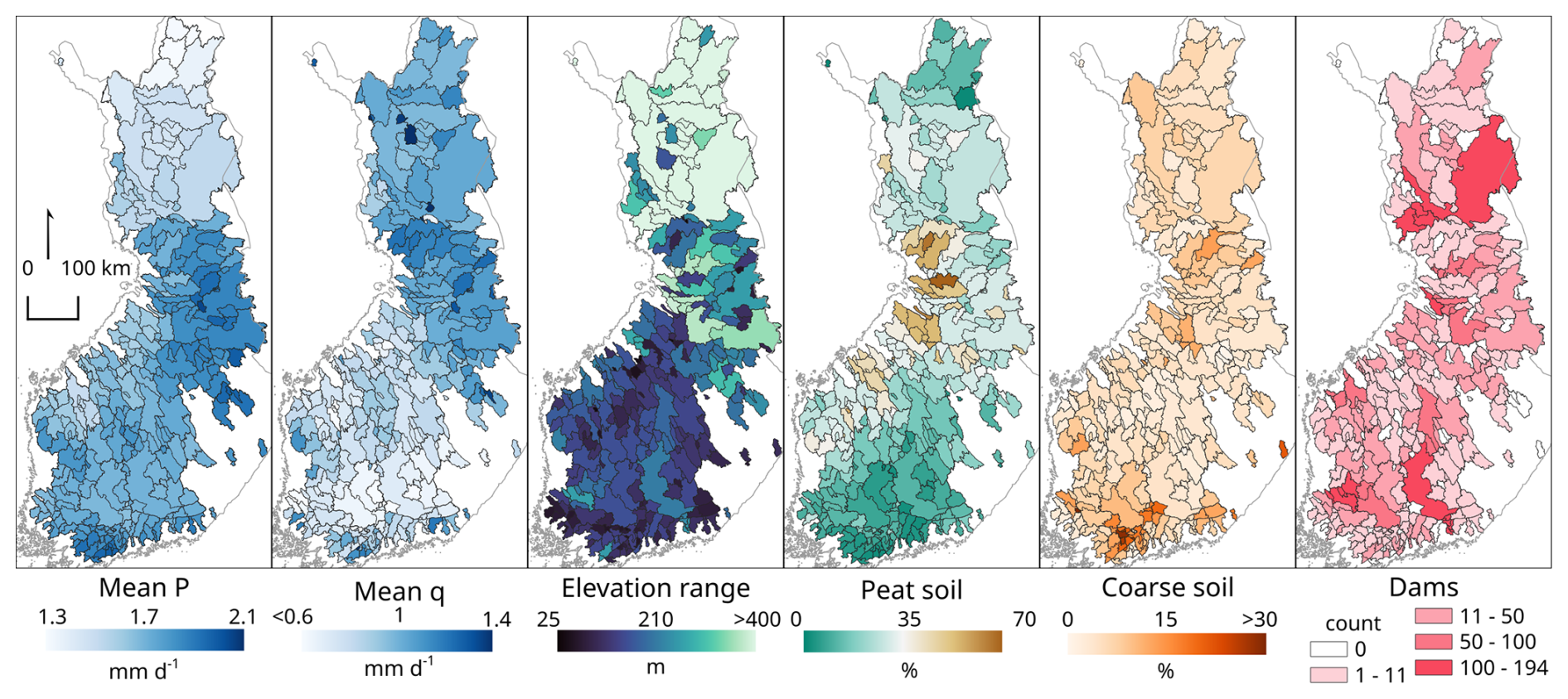
Figure 5 Multiple attributes exhibit great spatial variation over Finland. It should be noted that color scale for daily mean specific discharge starts from 0.6 mm d⁻¹, because the anomalously low discharges of gauge 3727 (0.19 mm d⁻¹) would have made variation of other catchments harder to see. Similarly, shown elevation range was capped at 400 m (max. 804 m) to keep variation outside of Lapland visible and coarse soil percentage was capped at 30 % (max. 48 %) due to a few small outlier catchments covered by major glaciofluvial deposits.

Eastern Finland and Lapland have considerably higher hills than the rest of Finland. Ostrobothnia has quite flat topography, which is accompanied by a large portion of the top layer of soil being peat, even in areas that support forests. The rest of Finland has varied topography with smaller, but relatively steep hills. Sandy and gravelly soils that are associated with terminal moraines and eskers are dispersed throughout the country but are especially concentrated on the southern border of the Coast and Lakes regions, which is also the reason for the general location of basin boundaries there. Catchments with the least human influence are limited in size and mostly located near headwaters.

6 Uncertainty and consistency of hydrometeorological observations

6.1 Quality of discharge values

The quality of discharge values varies both in time and between the gauges. Discharge measurements from (hydropower) dams have generally had high quality from the 1960s, as their geometry and discharge properties are well known and don't change. For other locations, the discharge values are based on more uncertain rating curves for the earlier decades. Rating curves started to be updated regularly every three years only in the 1990s for gauges maintained by SYKE. This may cause additional inaccuracies in the earlier decades due to changes in the morphology of the river channel. Actual discharge measurements that form the basis for the rating curve also improved substantially around the same time in large rivers due to the adoption of ADCPs (Korhonen, 2007). There is significant variation between different ELY centres in the quality of rating curves. Some are very close to SYKE, others do not update their rating curves as regularly.

The other component of quality affecting the discharge values is the accuracy of water level measurements. The water level accuracy of automatic limnigraphs that were used until 1990s was 0.5–2 cm, while the pressure sensors that have replaced them since have an accuracy of 0.1–1 cm. The effect of this on the discharge varies by gauge. Locations where small increase in water level corresponds to large increases in discharge, such as outlets of lakes, are most affected by this type of uncertainty. The water level measurements are validated monthly with manual measurements (Korhonen, 2007).

Three main quality checks are applied for non-hydropower gauges by SYKE. Firstly, water level observations outside of predetermined low and high thresholds are removed. The daily value is calculated if at least 60 % of the instantaneous values exist, and a day with any missing instantaneous values gets quality flag 108, missing instantaneous values. Finally, the daily discharge values are inspected manually once a year, and erroneous values are removed.

The wintertime raw discharge values are influenced by ice cover almost every winter for all of the gauges that are not part of a dam. The effects of ice are especially significant during ice jams. The wintertime discharge values are corrected (reducted) afterwards by an expert at the SYKE for 61 gauges in CAMELS-FI. Some of the gauges only receive occasional corrections for ice jam occurrences. Only one person has been appointed to handle the task at any time. When the person changes, new one is trained for the task, but the task is so manual that each person leaves their mark on the corrections. A computer-aided system has been in use since 1997, and the current system since 2008; previously the correction was done using a semi-logarithmic graph. Even the corrected values are inevitably less accurate than open channel values, with errors of 5 %–20 % common (Korhonen, 2007). Gauge metadata attributes include information of whether ice corrections are made for the gauge and discharge quality flags indicate periods that have been corrected (flag 3, reduction, see Appendix B).

6.2 The effect of short discharge timeseries to hydrologic signatures

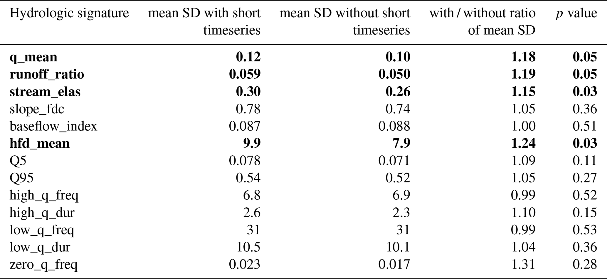
The effect of timeseries length of discharge observations to the stability of hydrologic signatures was investigated, because previous studies have shown that hydrological conditions between consecutive years can exhibit temporal autocorrelation (Lun et al., 2020; O'Connell et al., 2023). Thus, short time series may not represent long-term average conditions. Hydrologic signatures of each gauge with short (5–9 years, n=36) and medium (10–19 years, n=47) timeseries were compared to the group of five closest long timeseries (>20 years) gauges from the same hydrological region and regulation level. More specifically, the standard deviation (SD) of the signatures of the long timeseries group was calculated, and the change to the standard deviation was calculated when adding the shorter time series gauge to the group. This was repeated for all gauges with short or median timeseries and Welch's t-test (one-sided, α=0.05; Welch, 1947) was applied to see if there is significant overall difference between the SDs of the two groups. The results show that for mean discharge, runoff ratio, stream elasticity and mean half flow date, the shorter timeseries deviated significantly more from the long timeseries than the long timeseries deviated from each other, on average (Table 4). The effect on the same signatures was smaller, but still significant for gauges with medium length time series (Appendix E). Therefore, analysis of long-term conditions sensitive to these four signatures should preferably focus to timeseries of over 20 years. Conversely, five to ten years seems to be long enough for giving relatively stable estimates of the other hydrological signatures.

6.3 Agreement between different products

A simple comparison on the agreement of precipitation, PET and specific discharge as well as different snow products is presented here to probe the general agreement, or lack thereof, of different data sources. PET is on average larger in the boreal zone than actual evapotranspiration (AET) (Peltoniemi et al., 2015). This prevents comparisons that would directly calculate water balance using different subsets of precipitation, specific discharge and AET, since CAMELS-FI does not include AET estimates. However, some general agreement indicators can still be used. For example, over long timescales precipitation should always exceed specific discharge and difference of them should not exceed PET, assuming no water flows through catchment borders and water storages remain unchanged. These “bounded water balance” indicators were calculated for all catchments in CAMELS-FI using p_mean, pet_mean and q_mean meteorologic and hydrologic indices (Table 3). The meteorological and discharge data are within expected bounds for most of the catchments in CAMELS-FI (Fig. 3d). However, specific discharge exceeds precipitation for gauges 1369, 3335 and 3728. The gauge 3335 is probably explained by the mountainous terrain of the catchment, since it is a known issue that rain gauges underestimate precipitation during snowfall in windy conditions (Saltikoff et al., 2015). The other two catchments are heavily regulated and have relatively short observation periods within the reference climatological period 1991–2020, and thus changes to water storages are likely causes. PET is smaller than the difference of precipitation and specific discharge for gauges 1366, 3155, 3324 and 3727. Discharge is anomalously low for 3727 and the discrepancy is much smaller for the other three catchments. The reservoir lake of 3727 is also directly upstream of the reservoir of 3728, so they are strongly coupled. The gauge 1366 is heavily regulated, has a short observation period and is downstream of 3728 and 3728. 3155 has a similarly short time series and is heavily regulated. For gauge 3324, the cause is likely a large kettle lake (Sääksjärvi) that has been assigned to its catchment by the catchment delineation process based on surface topography. However, this kettle lake does not have an outlet stream, and is only drained trough groundwater. Thus it is likely that the lake is also “leaking” water to neighbouring catchments. Following our goal of inclusivity, we decided to not remove these catchments from the data, as they can still be useful for many tasks, and all had plausible causes for the discrepancies.

Table 3 Static attributes of the catchments in CAMELS-FI.

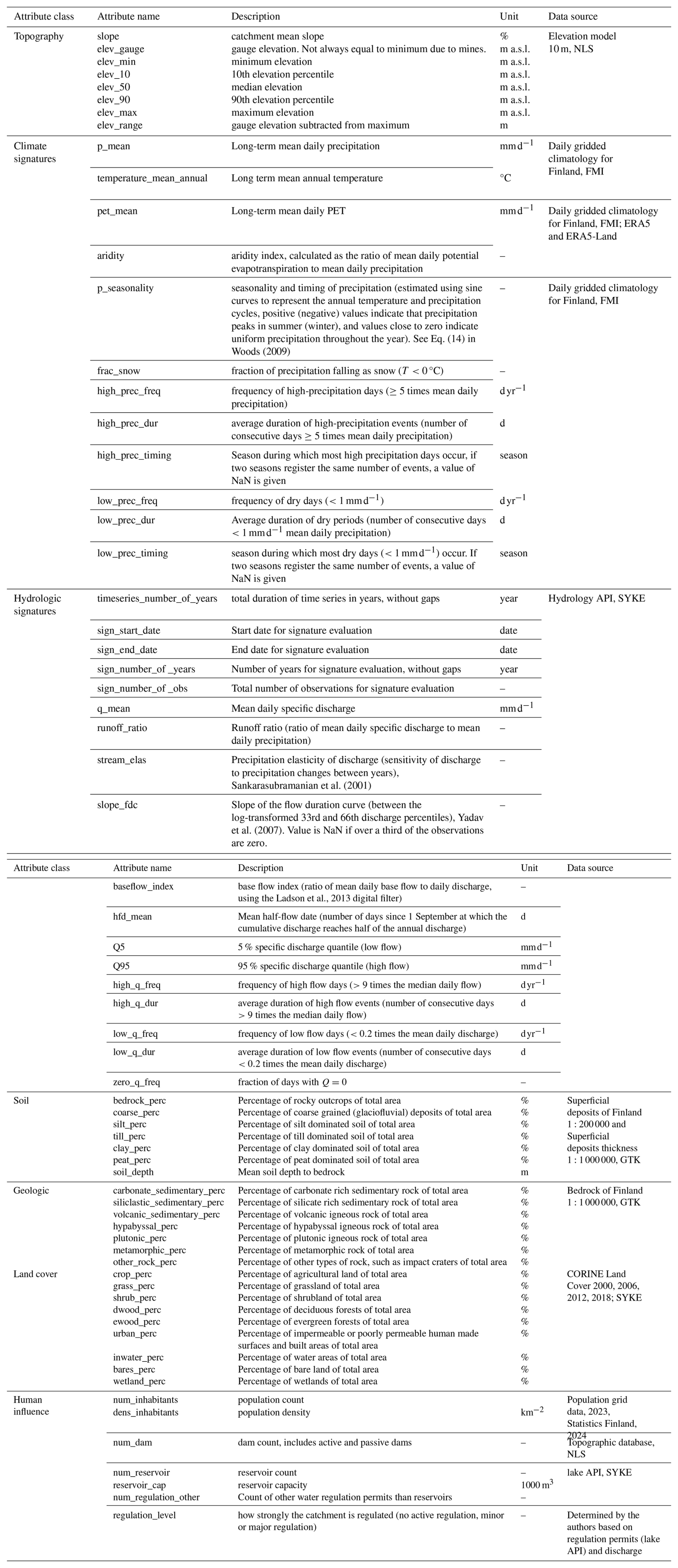
Table 4 The hydrologic signatures of gauges with short timeseries (5–9 years, n=36) differ more from nearby long timeseries gauges than the long timeseries gauges differ from each other, on average. However, the strength of the deviation depends on the signature. The significant (p<0.05) results are bolded.

The temporal consistency of combined PET was investigated for step changes, as it is a combination of different products. This was done by comparing the change in value when switching from one source product to another to the variation of those products four days before and after the change. In the autumn, the changes from one product to another are the same magnitude as the typical variation of the involved products and the typical variation is also low, less than 0.21 mm d⁻¹ for all source products. In the spring, the overall variation in the source products is higher around the changes from one product to another than in autumn. There is also a clear step change when transitioning from snow evaporation to FMI's PET, mean change 1.8 mm d⁻¹, which is approximately three times larger than typical variation of FMI's PET at that time of the year. However, while this change is too quick (one day), this sort of increase in potential evaporation when snow has melted is not completely unrealistic over slightly longer timescales, such as one week. Melting and evaporating snow has high albedo and prevents temperatures rising much above zero, while increasing the relative humidity of the air above. After the snow has melted, albedo lowers, temperature rises higher on sunny days, relative humidity lowers and plants start photosynthesizing (Betts et al., 2001). This leads to rapid increase in potential evaporation. It should be noted that actual evaporation can be considerably lower depending on land cover and water availability.

The FMI's snow depth and two SWE products, ERA5-Land and CCI3-1, were compared by counting the average number of snow days during water years 1991–2020. A day was considered a snow day if snow depth exceeded 1 cm, or SWE was over 1 mm. ERA5-land estimated on average 189.4 snow days, over three weeks more than CCI3-1 (161.9 d yr⁻¹) or FMI's snow depth (163.6 d yr⁻¹). This pattern holds generally in all parts of Finland. The similar averages of FMI's snow depth and CCI3-1 are probably explained by the fact that CCI3-1 combines ground station snow depth observations with microwave satellite observations (Takala et al., 2011). It should be noted that on the catchment level there is substantial variation between all products, which is probably due in part to the different grid sizes of the products and in part by methodological differences.

The values of the two SWE products were also compared by subtracting ERA5-Land from CCI3-1 (Fig. 6). ERA5-Land provides SWE values that are on average 11.3 mm higher than CCI3-1. However, the difference has exceeded 100 mm every year in the snowier parts of Finland. This is most likely caused by CCI3-1's known issue with severely underestimating SWE values higher than 150 mm due to limitations of microwave satellite measurements (Takala et al., 2011).

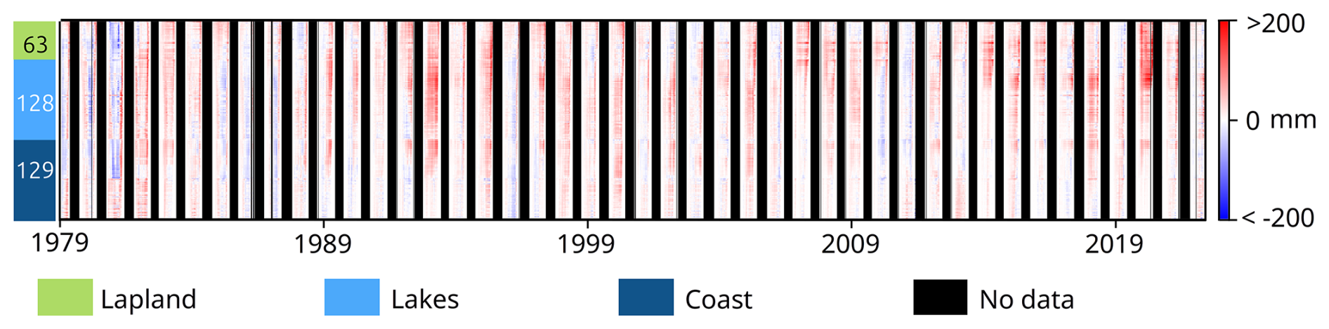
Figure 6 Difference between SWE estimates of ERA5-Land and CCI3-1. Positive (negative) values indicate that ERA5-Land is larger (smaller) than CCI3-1. Each row of pixels corresponds to one catchment and one column of pixels to state of all catchments at the same four day period (resampled from one day values due to resolution limitations of the figure). Gauges have been sorted vertically within regions by mean temperature.

Based on these results, we recommend using FMI's snow depth if SWE is not needed, and swe from ERA5-Land, in case the user only needs one snow data source. However, we would be cautious to place too much trust in ERA5-Land, since it estimates too long snow periods.

7 Data availability

CAMELS-FI can be accessed at Zenodo under https://doi.org/10.5281/zenodo.15853357 (Seppä et al., 2025). All the code produced for creating CAMELS-FI is available at the dataset's code repository at https://doi.org/10.5281/zenodo.21101162 (Seppä and Sainio, 2026). Please note that the process involved some manual work, which means that the data are not fully reproducible by code alone.

8 Conclusions

This study introduces CAMELS-FI, a large-sample, open-source catchment dataset for Finland, encompassing 320 catchments. CAMELS-FI provides a consistent, high-quality, comprehensive and easily usable dataset of daily hydro-meteorological time series and attributes on topography, land cover, anthropogenic influence, climate, hydrology and soil for a diverse set of catchments. The dataset follows the format of other CAMELS datasets, especially those from Great Britain, Switzerland and Sweden, as closely as possible, facilitating cross-dataset comparisons and software integration.

The dataset's extensive spatiotemporal coverage and detailed attributes advance cold region hydrological science by:

• I.

  Facilitating robust large-scale studies on the impacts of snow, ice and lakes on water cycles, and the hydrological responses to climate change in northern latitudes.

• II.

  Enabling the training of state-of-the-art rainfall-runoff deep learning models, which could lead to e.g. improved flood mitigation, enhanced water resource management and more efficient hydropower production.

• III.

  Conserving time of researchers from complex and computationally expensive preprocessing of data.

• IV.

  Offering a common dataset for benchmarking performance of different models in snowy and lake-dominated catchments.

While CAMELS-FI offers a wealth of data, there are opportunities for future expansion and enhancement. These include adding new types of information, for instance morphometrics or water quality attributes, such as phosphorus, nitrogen or carbon loads. We believe the simple structure of the dataset makes adding new attributes straightforward, and we also encourage possible expansions to be shared openly. Another possible development opportunity would be integrating CAMELS-FI with the announced CAMELS-Nordic (Valseth et al., 2025), since Sweden, Norway and Finland share many cross-border datasets. This would also allow including many of the cross-border catchments that were excluded from CAMELS-FI.

Appendix A: Class generalizations

Table A1 CLC lvl three classes used for each land cover class in CAMELS-FI. Please note that some of the classes are not present in all editions.

Table A2 GTK's soil classes that were combined for CAMELS-FI.

Appendix B: Time series

Table B1 Value ranges of time series variables.

Table B2 Discharge quality flag classes.

Appendix C: List of CAMELS and related datasets

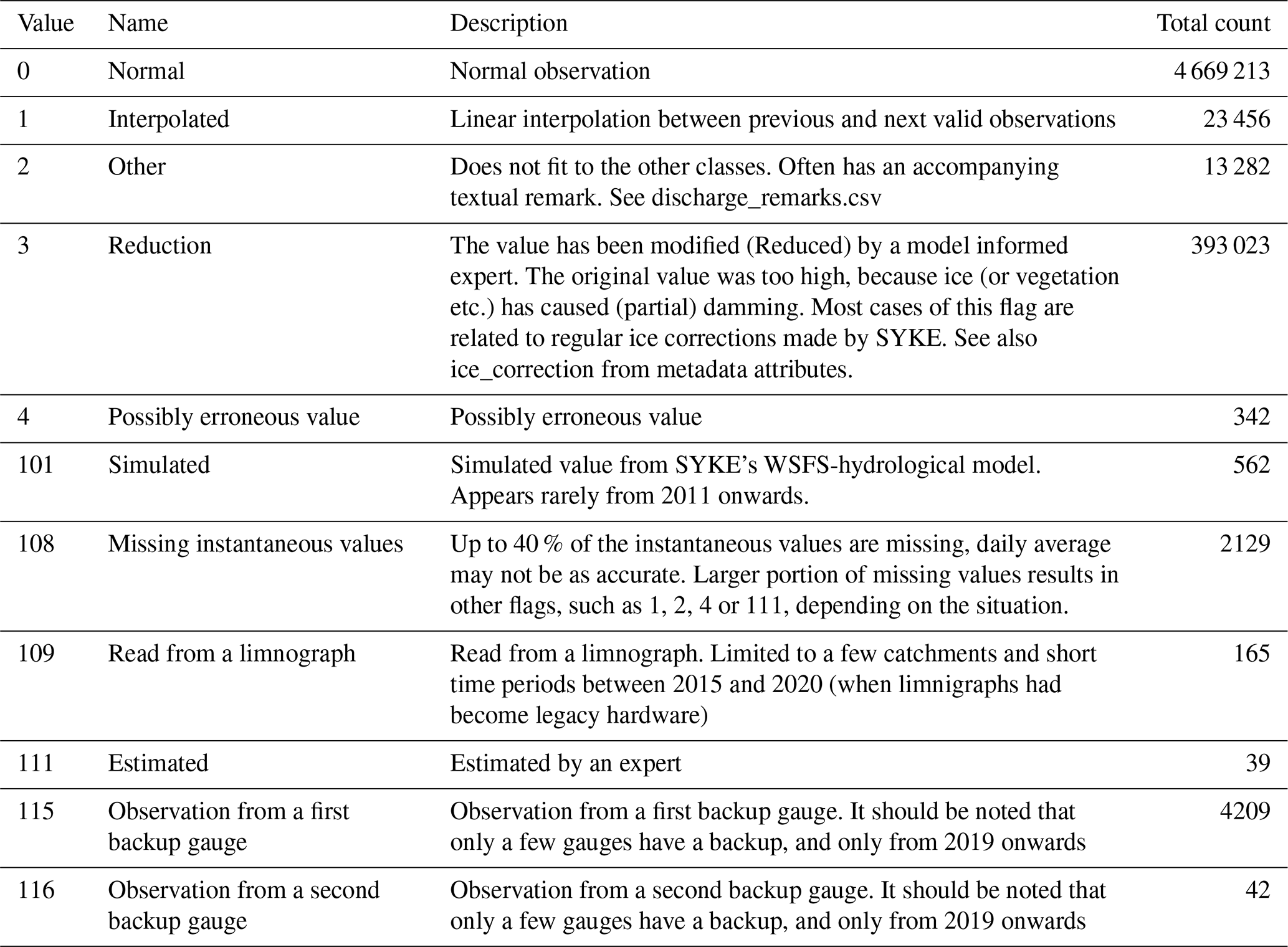
We conducted a literary search of the existing CAMELS datasets and closely related datasets by

1. searching Web of science with the phrase: “CAMELS-”* AND dataset

2. searching Web of science with the phrase: “LamaH-”* AND dataset

3. searching google and google scholar with: CAMELS dataset

4. searching “CAMELS” and “LamaH” from Earth System Science Data and Scientific Data, two most common journals for the publication of these datasets.

5. Searching for other datasets from the references of found datasets

Last date of searching was 24 February 2026. Please note that the rapid increase in the count of CAMELS datasets means that this list is likely to become outdated quickly. This is why we also created a github-repository, that can be updated to match future additions (https://github.com/iiroseppa/camels-dataset-list, last access: 25 February 2026).

Table C1 CAMELS datasets.

Table C2 CAMELS-related datasets.

Appendix D: Map of Toponyms

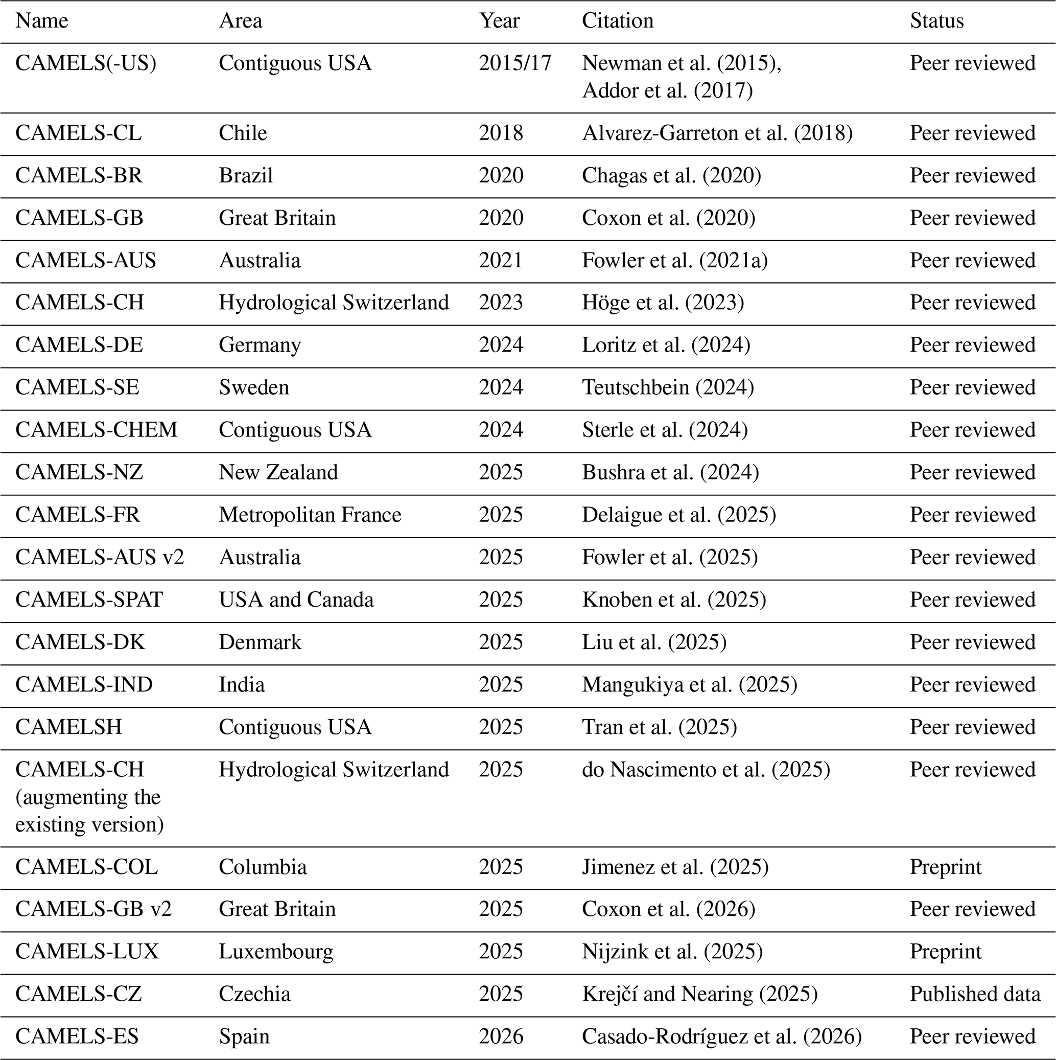
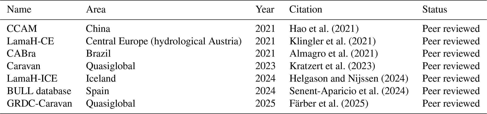
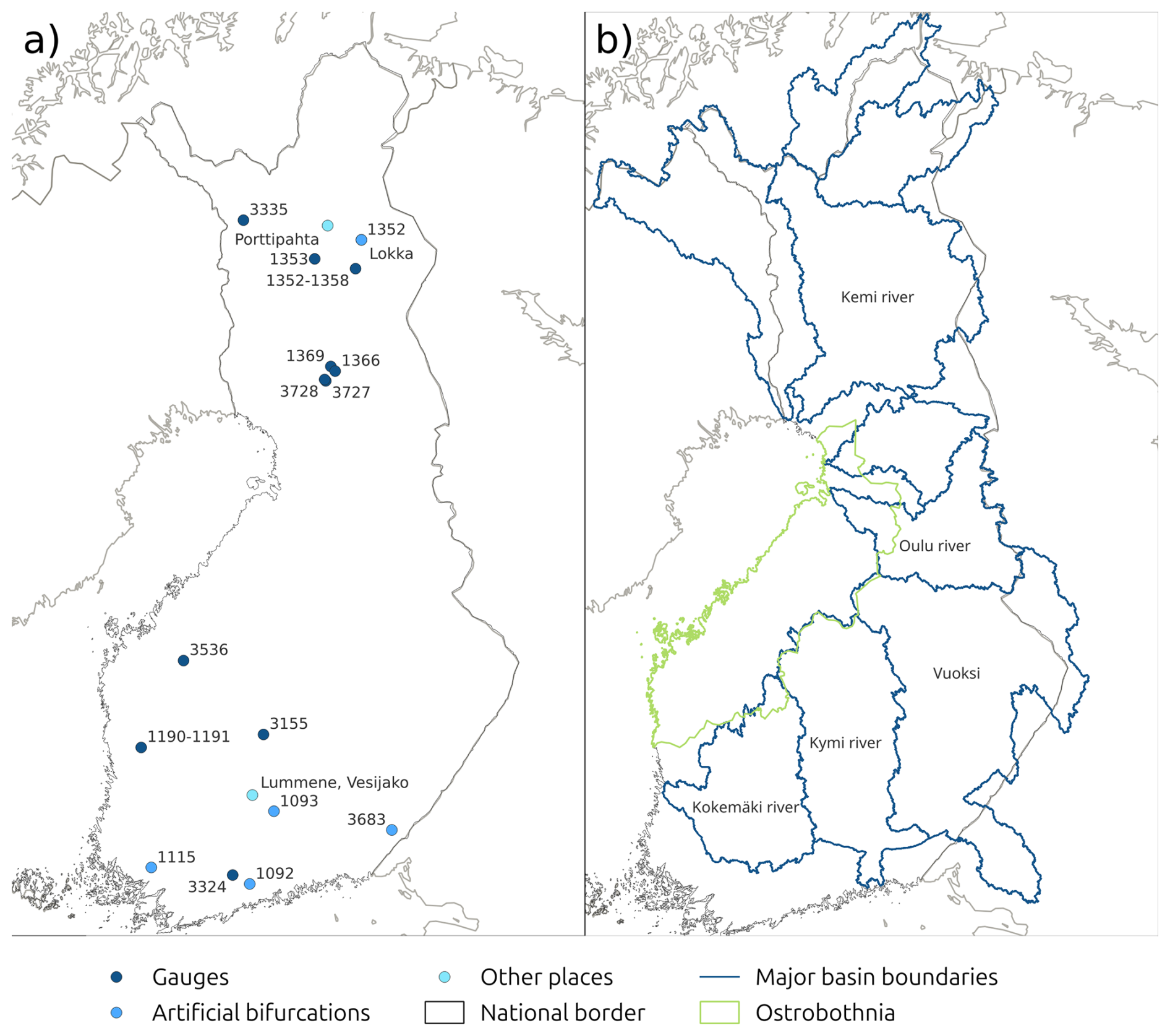
Figure D1 Places mentioned in the text. (a) Small locations. (b) Major basin boundaries and the Ostrobothnia region.

Appendix E: Hydrologic signature stability of medium length (10–19 years) hydrological timeseries

Table E1 Hydrologic signature stability of medium length (10–19 years) hydrological timeseries. See Sect. 6.2 for further details. The significant (p<0.05) results are bolded.