the Creative Commons Attribution 4.0 License.
the Creative Commons Attribution 4.0 License.
 | 26 Jun 2026
BEACH: Barbados and Eastern Atlantic Combined High-altitude dropsonde datasets
Helene Marie Gloeckner
Theresa Mieslinger
Nina Robbins-Blanch
Geet George
Lukas Kluft
Tobias Kölling
Sandrine Bony
Julia Miriam Windmiller
Bjorn Stevens
As part of the ORCESTRA field campaign in August and September 2024, 1191 dropsondes were deployed over the Eastern and Western Atlantic ITCZ from the HALO aircraft coordinated by the PERCUSION and MAESTRO subcampaigns. Here, we describe the hierarchy and processing of the resulting Barbados and Eastern Atlantic Combined High-altitude (BEACH) dropsonde datasets. The Level 0 dataset contains measured meteorological variables, such as relative humidity (RH), temperature (T), pressure (p), eastward (u), and northward (v) wind data as output by the AVAPS system. The corresponding ASPEN quality-controlled data is called Level 1. Level 2 adds further measurement-specific quality control flags. Level 3 builds the core of BEACH including all quality controlled dropsonde profiles interpolated to a common 10 m altitude grid and concatenated into a single dataset. We further derive mesoscale vorticity, divergence, and vertical velocities from 87 circular flight patterns in Level 4 using the regression method. These area-averaged variables will guide our understanding of mesoscale processes acting within the ITCZ, one of the main goals of ORCESTRA. All data levels are openly available on IPFS, while the processing code is made public on GitHub.
- Article
(6890 KB) - Full-text XML
- BibTeX
- EndNote


The Organized Convection and EarthCARE Studies over the Tropical Atlantic (ORCESTRA, Stevens et al., 2026) field campaign was designed to quantify drivers of mesoscale convective organisation in the tropics with a particular focus on the structure and variability of the Atlantic Inter-tropical Convergence Zone (ITCZ). More than 1000 dropsondes were launched as part of PERCUSION1, and in support of the MAESTRO campaign, two of the sub-campaigns of ORCESTRA. The soundings were conducted in August and September 2024, and later processed to derive area-averaged estimates of horizontal divergence and vertical velocity on the mesoscale (∼ 200 km, 1 h; close to the meso-β scale as per Orlanski, 1975). The datasets described here provide the first comprehensive mesoscale vertical velocity estimates derived from airborne dropsonde measurements within the Atlantic ITCZ.
Reliable profiles of the area averaged vertical wind velocity, W(z) are crucial to determine the magnitude and sign of vertical moist static energy advection in the tropics, which in turn helps to understand the interactions of cumulus convection with large scale circulations (Back and Bretherton, 2006), and patterns of tropical rainfall (Bernardez and Back, 2024). Directly measuring W, however, remains challenging due to its small magnitude compared to the horizontal wind components. While reanalysis data provides estimate of W, without independent measurements it is hard to know how well these estimates are constrained by data, even in cases when additional data from field campaigns are assimilated (Huaman et al., 2022).
Efforts to derive W directly from observations have a long history. Already eighty years ago Panofsky (1946) proposed integrating area-averaged divergence of the horizontal wind velocity (𝒟) upward from the surface to compute W. An approach Bellamy (1949) developed further to graphically acquire divergence from three dislocated measurements which defined a triangle. From Gauss' theorem, the area averaged divergence is equal to the line integral of the normal wind around the perimeter of a polygon, whose vertices can be defined by point measurements from sondes. Ceselski and Sapp (1975) adopted this approach to derive 𝒟 from operational soundings over the Northern American continent. Yanai (1961) applied these methods to sounding measurements to provide the first estimates of W in the tropics. The utility of this approach was demonstrated in subsequent analyses of the tropical atmosphere (Reed and Recker, 1971; Yanai et al., 1973), during GATE, and in a great many field studies thereafter, as sounding arrays increasingly became incorporated in the design of field campaigns.
Panofsky and Bellamy's ideas were recast by Lenschow et al. (1999), who applied them to aircraft data. Lenschow and collaborators used airborne gust-probe measurements of the horizontal wind to estimate 𝒟 at the top of the boundary layer from straight and level legs arranged to close a polygon. They argued that circular flight patterns would be preferable, as they not only minimize the perimeter to area, but also avoid sharp turns required to transition between polygon edges, during which measurements are not useful. Lenschow et al. (2007) demonstrated the circle method to calculate 𝒟, and showed that 𝒟 could equivalently be computed from spatial derivatives estimated from best fit linear-regression of the measured wind field to spatial distance.
Bony and Stevens (2019) combined the past approaches by using an aircraft to deploy dropsondes to construct a sounding array. By flying multiple circles with a diameter of approximately 200 km following the mean wind they could provide independent estimates, and hence quantify the error. This allowed them to demonstrate that about twelve sondes were sufficient to derive a reliable mesoscale divergence profile and 6 to 8 sondes are tolerable to evaluate the structure of the calculated vertical velocity profile. Bony and Stevens (2019) also demonstrated that their measurements were amenable to the regression method. Using the ICON model to perform large eddy simulation for the observed conditions, they further demonstrated that the temporal decorrelation of the divergence is given by the advective timescale, and hence much less than the time required to fly a single circle.
As compared to the use of winds measured just at flight level, the use of dropsondes has the advantage of sounding arrays, in that they provide vertical profiles of 𝒟, and hence W. Hence these methods were incorporated into the experimental design of EUREC4A (Bony et al., 2017) and other campaigns (Pincus et al., 2021) in the winter trades, as well as for HALO-(AC)3 in the Arctic (Wendisch et al., 2024). During the 2019 OTREC field campaign (Fuchs-Stone et al., 2020; López Carrillo and Raymond, 2011), the regression methods were generalized to a variational approach by which 𝒟 and W were estimated from dropsonde data (Vömel et al., 2020) spread over a large area augmented by winds estimated from airborne doppler radar measurement following Mapes and Houze Jr. (1995).
Methods to estimate W continue to evolve. Poujol and Bony (2024), for instance, have developed qualitatively new approaches to estimating W, by tracking humidity gradients in time using satellite measured radiances. Their method, however, requires an area devoid of cloud, making its application within the ITCZ problematic. Hence to expand our understanding of convective regimes, PERCUSION incorporated circular flight patterns to drop sondes in and around the Atlantic ITCZ and thereby quantify W. These measurements resulted in the Barbados and Eastern Atlantic Combined High-altitude (BEACH) datasets described in this paper. A name chosen in part because it extends the musical themes of other named elements within ORCESTRA through reference to Amy Beach, the first female US American composer to publish a symphony.
In what follows we present BEACH and the choices made in its construction. Section 2 outlines the dropsonde measurements during PERCUSION. Section 3 describes the methodological and technical details for the data processing, which is adapted from the JOANNE processing described in George et al. (2021). Section 4 gives a brief overview of the thermodynamic and dynamic structure of the tropical atmosphere as measured by the BEACH dropsondes.
During PERCUSION 1191 sondes were dropped from the German research aircraft HALO. Data of 715 sondes, launched between 27 August and 28 September, was assimilated into the IFS analysis. After quality control and other processing steps described in Sect. 3, 1115 sondes were used in the BEACH Level 3 gridded product. Most of these were grouped in 89 circles to form the BEACH Level-4 product.
Detailed sonde statistics for each flight are provided in Table 1, and the circles that were flown in coordination with the MAESTRO subcampaign are listed in Table B1 in the Appendix. Flight tracks were designed with two major objectives: (1) to fly along the EarthCARE track coincident with an EarthCARE overpass to calibrate the satellite measurements and validate the retrievals, and (2) to provide estimates of the mesoscale vertical motions in and around the ITCZ (see Sect. 3.4).
Table 1PERCUSION dropsonde statistics showing the number of sondes per flight and processing level.
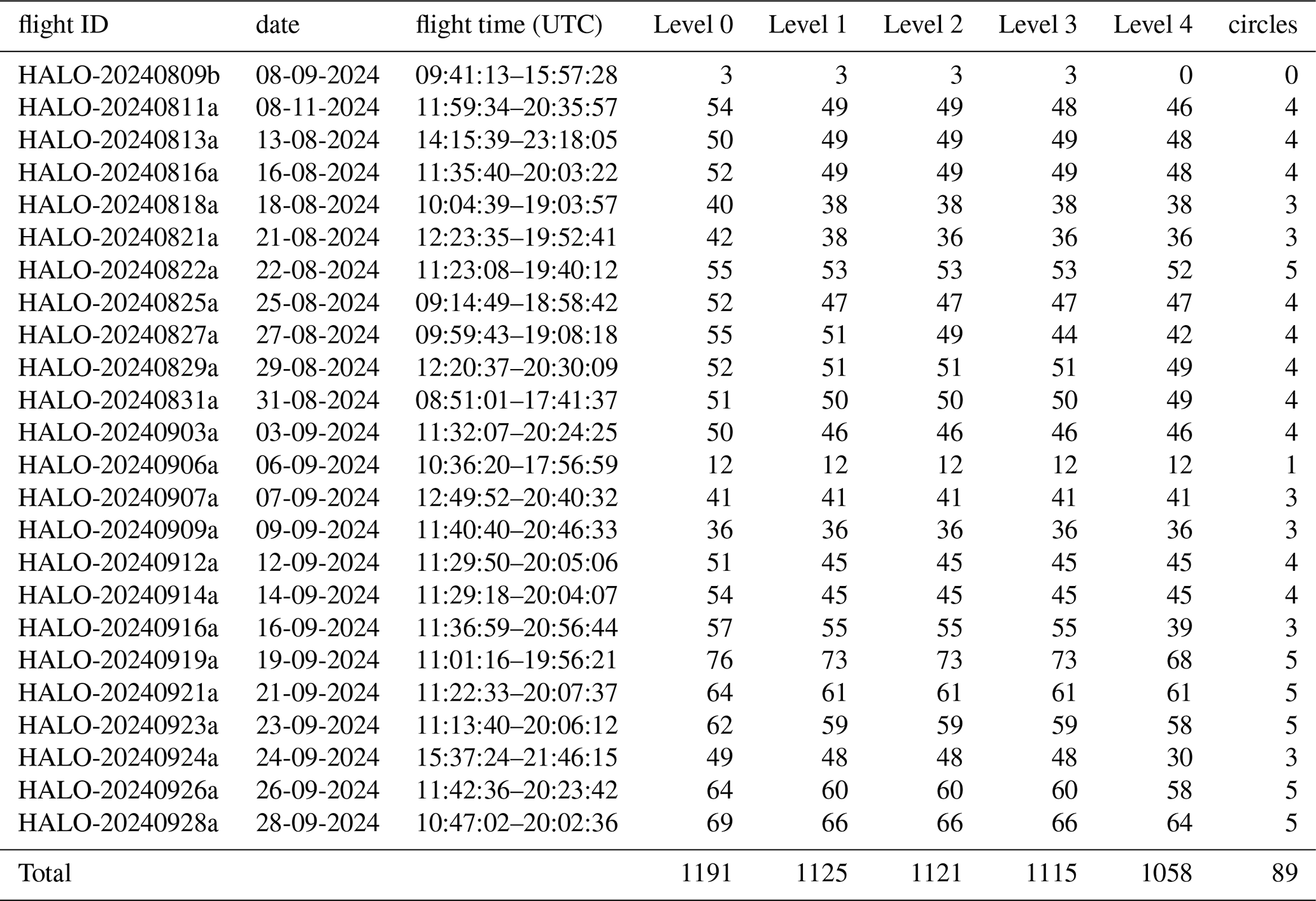
The circles were designed to take approximately one hour at 14 km altitude to complete, which resulted in a circle diameter of roughly 260 km, which varied slightly based on flight altitude and hence speed. Additional circles with a smaller diameter of ≈ 140 km were flown at lower altitudes in approximately 40 min to coordinate with MAESTRO measurements by the SAFIRE ATR-42 research aircraft near the Cape Verde island Sal, leading to a larger variation in circle diameter in the East.
A typical flight in the East included four circles: one near the center of the ITCZ, two at the edges and one in coordination with the SAFIRE ATR-42. During flight planning the ITCZ was identified as the region where total column water vapor values exceeded 48 mm or where surface wind direction changed (Praturi and Stevens, 2026). However, especially in the West, the ITCZ was often not well defined (Stevens et al., 2026), as regions of elevated water vapor could extend over a wide range of latitudes. Even with a clearly defined ITCZ, restrictions from air-traffic control sometimes did not allow the orientation of the circles along the EarthCARE orbit and across the ITCZ. As a result, in the West the flight plans focused on distributing circles within and across the ITCZ, with less regard to the orientation of the circles, except to maintain a similar inter-circle distance as in the East, and remain anchored to EarthCARE's overpass.
Figure 1 shows all sondes with measurements that passed the basic quality control colored depending on whether they belong to a standard one-hour circle (teal), a smaller ATR circle (yellow), or were dropped in coordination with measurements by the research vessel R/V Meteor (navy). In total, 90 circles that were planned to have dropsondes were flown of which 87 have enough sonde measurements to derive vertical motion on the mesoscale (Bony and Stevens, 2019, see Sect. 3.4). The indicated regions East, North and West are the same used in Stevens et al. (2026) and are used in Sect. 4 to divide the data. Additional sondes were sometimes dropped at the point of the EarthCARE overpass, and at the Southern or Northern most point of the overpass to validate other instruments, and for instrument calibration on board of HALO. On flight HALO-20240919a2 many sondes were dropped along the flight path to provide a basis for testing a variety of sampling strategies. On this flight alone 73 sondes were launched, one on average every 7–8 min.
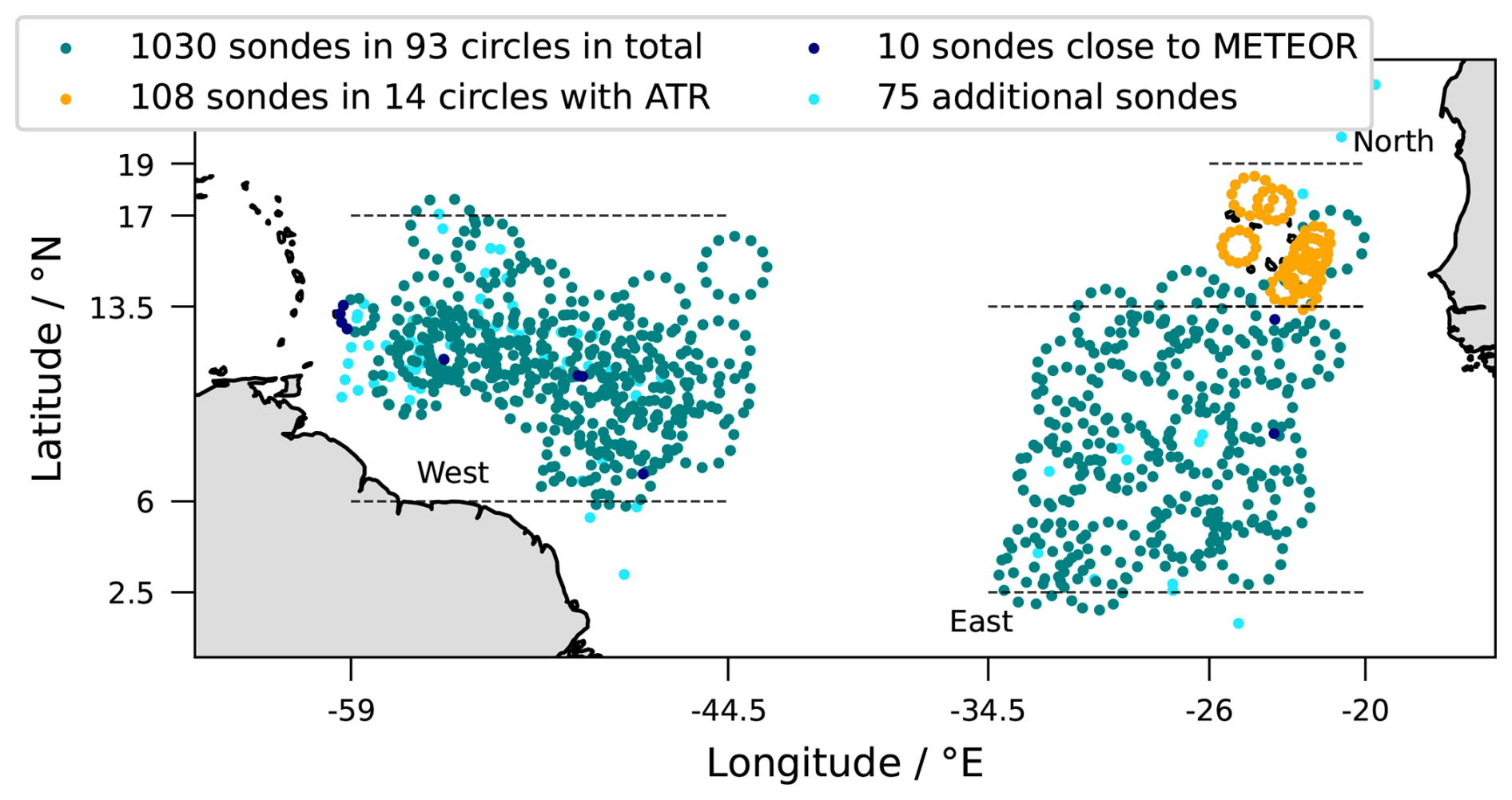
Figure 1Location of dropsonde launches. Sondes that were launched in ATR coordinated circles are marked in yellow, sondes in regular circles in teal, and sondes that were dropped close to the R/V Meteor in navy regardless their affiliation to a circle. Other sondes are marked in light blue. Sondes can be part of multiple groups (i.e. the sondes in coordination with the ATR were usually also part of a circle and hence appear twice in the legend).
2.1 Instruments and Sensors
The dropsondes used during PERCUSION are of the type RD41 developed by NCAR (Hock and Franklin, 1999; Aberson et al., 2023) and manufactured by Vaisala. Each sonde consists of a PTU unit measuring pressure, temperature, and relative humidity (RH) at 2 Hz sampling frequency. A GPS unit provides information on the dropsonde position at 4 Hz, and wind components are derived from the horizontal displacement of the sonde on its way to the surface. The dropsonde system during PERCUSION could receive data from 8 sondes simultaneously, but usually no more than 6 sondes were in the air at once. After the drop, different sensors need different equilibration times until the measurements are valid. The Aspen default equilibration times, that were used in the processing, are listed in Vömel and Goodstein (2020) and more details on single sensors, their resolution, and performance are given in George et al. (2021) and their Table 1.
The dropsonde sensors are the same as those included in radiosondes of type RS-41 launched from Barbados, and the RV METEOR as part of ORCESTRA. These radiosondes in addition to the radiosondes launched at INMG populate the RAPSODI datasets (Winkler et al., 2026). Common variables and a uniform grid that is shared among RAPSODI's Level 2 and BEACH's Level 3 facilitate a combined analysis, even though the processing described in Sect. 3 differs significantly between the datasets due to different raw data formats and dataset requirements.
2.2 Problems during operation
After HALO-(AC)3 (Ehrlich et al., 2025), the last HALO campaign with extensive dropsonde operations before PERCUSION, the antenna for the dropsonde receiver on HALO was moved from a central position on the bottom part of the fuselage behind the wings of the aircraft to the port-side wing. As a consequence, a longer cable and an amplifier were installed to connect the antenna with the AVAPS system. The connection between sondes in the air and the AVAPS system seemed interrupted during flight maneuvers with high roll angles possibly due to the shift in antenna position. In addition, the network connection from the AVAPS system to the dropsonde computer was unstable until 14 September 2024 which led to data loss from some sondes in the air on HALO-20240827a and HALO-20240914a. Overall those problems did not lead to significantly worse quality control drop outs than experienced during EUREC4A (Sect. 3.2).
In some instances, air traffic control restricted drops during flight operations resulting in circles with fewer sondes. In some of these instances, parts of the circle could be reflown a second time, or additional sondes could be dropped to cover a wider area (e.g. see flight reports for HALO-20240907a or HALO-20240926a). In one instance, on flight HALO-20240821a, clearance to drop sondes was revoked during an entire circle, and it therefore remains without sondes.
In three cases, two measurements have the same serial ID in the raw data file headers. This can happen if a sonde is initialized twice without a drop in between, if the power-pin of a sonde is removed and re-plugged within a few milliseconds because this leads to a factory reset of the sonde, or if two sondes are initialized to send data on the same frequency and the frequency is changed at a later stage for one of those sondes. In case of a factory reset, the sonde forgets its calibration and the serial ID 000007500 is assigned to it. To handle the above mentioned specific cases, BEACH uses a hash derived from the serial ID and launch time to uniquely identify each sonde.
The datasets in BEACH (see Fig. 2) are organized in five levels: Level 0 contains the raw data as recorded by the AVAPS system; Level 1 contains ASPEN-processed netCDF files; Level 2 includes further customized quality controlled Level 1 data in zarr format; Level 3 consists of the Level 2 data interpolated onto a common altitude grid, as well as additional derived physical variables; Level 4 associates Level 3 data with circles and provides circle products, e.g., the mesoscale vertical motion.
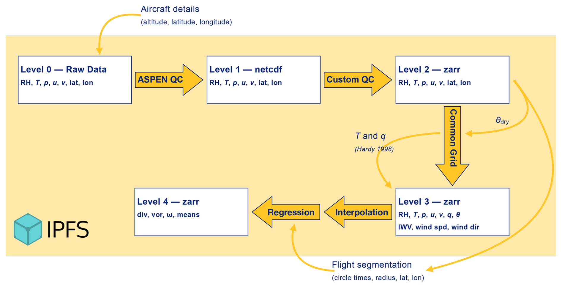
Figure 2Schematic overview of the data processing from the AVAPS raw data to the Level 4 circle products.
All processing steps generating the BEACH datasets are openly available and embedded in the Python package https://github.com/atmdrops/pydropsonde. The BEACH datasets were created with pydropsonde version 0.5.5 which evolved out of the processing done for the JOANNE dataset (George et al., 2021). The basic structure of the data levels remains, while some parts of the processing have been improved and expanded, as will be described in this section.
3.1 Level 1 processing: ASPEN quality control
The Level 0 (Gloeckner et al., 2026a) or raw data generated by the AVAPS system is described by George et al. (2021, Chapter 2.3.1 and Table 4). pydropsonde uses the raw data files “D-files” and the metadata files “A-files”. As a first step, the metadata of each sonde is checked for a detected launch, which occurs if the sonde launch detect pin has been activated. The respective “A-file” includes a line stating “Launch Obs Done?” and possible flag values “0” – False and “1” – True. In case the parachute does not open, or the opening is not detected, the sonde does not switch to a high power mode for transmitting data and the connection to the receiving unit is lost after falling a few hundred meters. Such profiles are of little value and discarded from any further analysis.
ASPEN is a software package developed by NCAR that is used for analysis and quality control (QC) of dropsonde data. For the BEACH processing, ASPEN version 4.0.4 was used. For each sonde that detected its launch, the ASPEN software (Martin and Suhr, 2021) is run on the raw data (D-file) using a container-based approach. A docker image containing the command-line functionality of ASPEN is utilized within the processing pipeline with the default editsonde configuration. The ASPEN processing includes several quality control steps, such as removal of the equilibration period, smoothing, and outlier checks as described in the ASPEN Manual (, ) and Dropsonde Data Quality Report (Vömel and Goodstein, 2020, based on the NRD41 sondes, which are built differently but contain the same sensors).
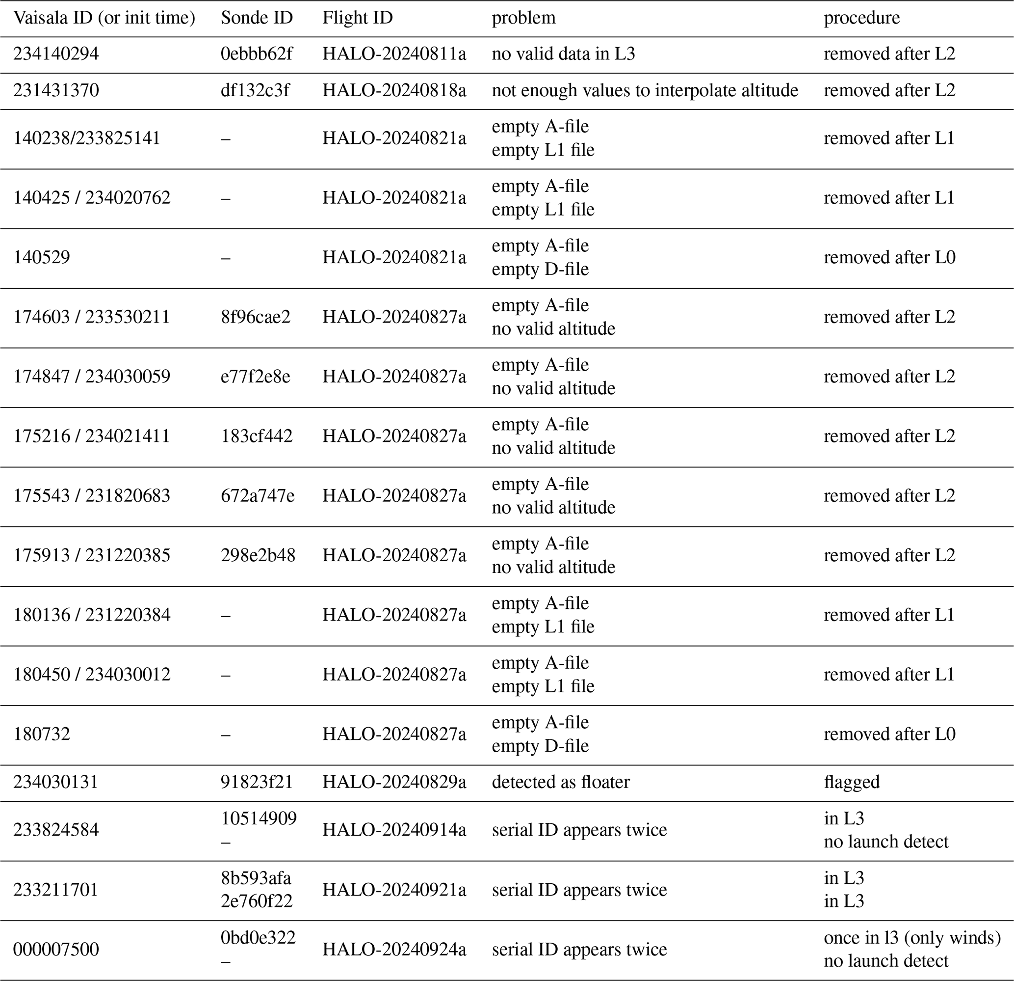
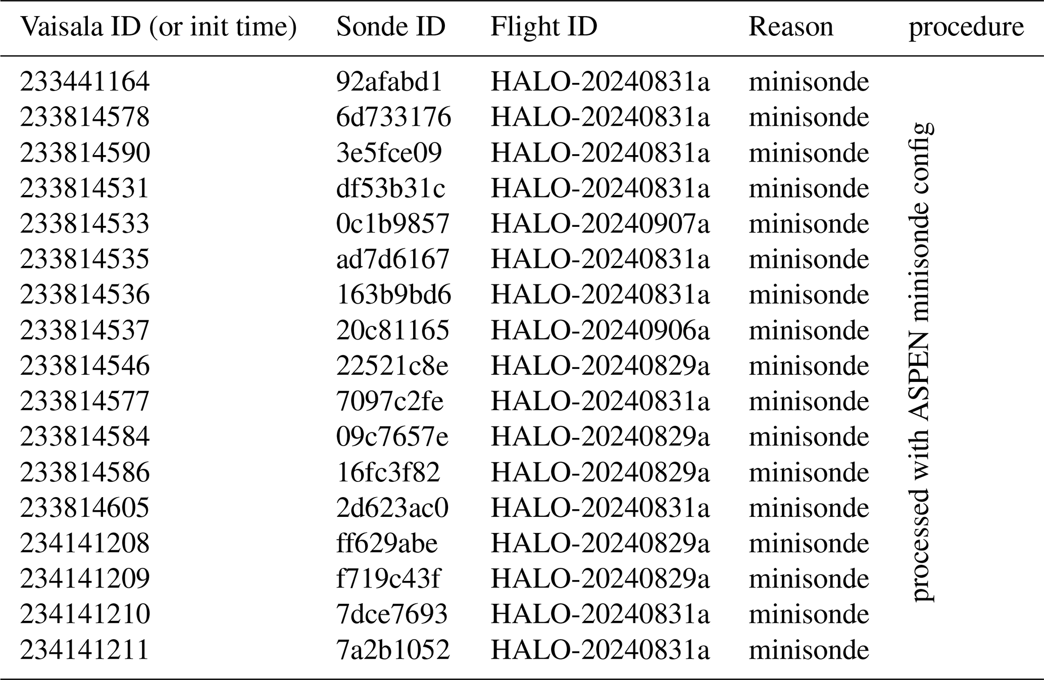
We encountered several special cases due to connection or manufacturing issues that needed individual treatment: Eleven sondes were missing metadata information due to an empty A-file. Since the processing with ASPEN is independent of the A-files, it was applied regardless. A flag stating a successful launch-detect is set to “None” within the pydropsonde processing in those cases signaling that the status of launch-detect is unknown. Since all of those sondes have other problems as well, neither of them appears in Level 3 (see Table E1 in the Appendix). Five of those sondes have a Level 2 file, but should be handled with care since their altitude coordinates are unreliable. They can be identified by a NaT launch_time. In addition, based on the metadata, 17 sondes were falsely configured by the manufacturer to be of type NRD41, often called minisonde, instead of the actual sonde type RD41. They have been processed by ASPEN with the respective minisonde configuration, because ASPEN does not allow a processing with the default RD41 configuration for those sondes. While this does not influence the variables used for the BEACH datasets of Level 3 and above, it does impact the estimated vertical wind component included in the Level 1 and 2 datasets of those sondes. The affected sondes are listed in Table E2 so that they can be manually reprocessed if needed.
In total, 1125 sondes reached Level 1 (Gloeckner et al., 2026b) with individual numbers per flight listed in Table 1. We call the untouched ASPEN netCDF output files Level 1 data and store it in form of single datasets per sonde.
3.2 Level 2 processing: Additional quality control
3.2.1 Quality Control Tests
The Level 2 (Gloeckner et al., 2026c) processing applies additional quality control (QC) tests to provide a basis for a combined analysis of all profiles. It includes four variable-specific tests that we call profile-sparsity, profile-extent, near-surface-coverage, and sfc-physics. Before those tests are run, we remove data above the drop height (gpsalt-below-aircraft). The tests are based on the JOANNE processing (George et al., 2021) with slight modifications and additions, described in Sect. 3.5.
-
Filter: gpsalt-below-aircraft: The ASPEN Level 1 data contains the altitude variable
gpsaltobtained from GPS measurements. Depending on the GPS connectivity within the aircraft, the GPS measurements need an equilibration period of up to 10 s (Vömel and Goodstein, 2020) to build up a connection after a sonde launch. The ASPEN-processing removes this period from the u and v data, but not from the GPS-altitude (gpsalt) data points, such that sometimes erroneous measurements above the aircraft altitude are included before the connection is established. Therefore,pydropsonderemoves thegpsalt, u, v, sonde latitude, and sonde longitude values for any measurement with agpsaltabove the aircraft altitude as measured by BAHAMAS (Konow et al., 2021). This is a valid approach because the sondes were not carried upwards in the ORCESTRA measurements. The data is removed before any other QC tests, such that their results are not influenced by a faultygpsalt. -
QC: gps-valid: A second QC checks whether the u and v measurements have an unusually large variation. It is failed if
exceeds three times the mean σuv of all sondes: , because large σuv values indicate that the GPS measurements are faulty, either due to fast falls or large gaps in the GPS measurements.
-
Profile Fullness: This is checked with three variable specific tests: The profile-extent is passed if the highest valid measurement of a sonde is above 8000 m. The profile-sparsity test is passed if less than 20 % of the theoretically available data is missing. This is an adapted version of the profile-fullness-test (sat-test) in George et al. (2021). The near-surface-coverage test is passed if 50 or more measurements have been made in the lowest 1 km. The altitude measurement used depends on the variable, since u and v have
gpsaltas their reference altitude, while p, temperature, and RH havealtas their reference altitude in the Level 1 data. Figure 3 shows the histograms for the QC tests that determine the profile fullness of a measured variable. It shows, that the horizontal wind measurements have a larger fraction of missing values than the PTU measurements and that the relative humidity sensor needs a longer time to equilibrate, resulting in lower profile extents. -
QC: sfc-physics: In addition to those QC tests which are aimed to check the fullness of a profile, the bottom-most value in each profile is checked for physical plausibility; i.e. the check is passed if the lowest RH measurement exceeds 0.3, the lowest temperature measurement is above 293.15 K, and the lowest pressure is between 1005 and 1020 hPa. Those thresholds were chosen relatively lax and for a tropical atmosphere. They should be chosen differently for dropsondes in other locations, as for example during HALO-(AC)3. Two things can lead to a failed sfc-physics test: (i) the sonde did not send data until it reached the surface; and (ii) there was a calibration issue. In the first, more common, case the near-surface-coverage test is failed as well. The second case was only triggered for a single sonde (0bd0e322 on HALO-20240924a), which was unintentionally factory-reset as described in Sect. 2.2, and consequentially has a shifted temperature profile and anomalously low RH measurements. The corresponding values have been masked in Level 3 so as to not adversely impact other calculations.
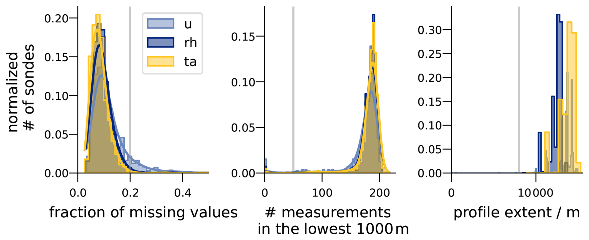
Figure 3Normalized sonde counts for the quality measures. Grey lines denote the thresholds for a sonde to pass a QC (i.e. a sonde is flagged if the fraction of missing values exceeds 0.2, if the number of near-surface measurements is lower than 50, or if the profile does not extent above 8000 m). QC values for v are equal to those from u. QC values for p are indistinguishable from QC values for ta for the purpose of the plot and omitted for readability.
3.2.2 Variables in Level 2
For Level 2, all sondes are concatenated along the time dimension into a dataset with a ragged array data structure (Brian Eaton et al., 2024) with dimensions time and sonde. The times_per_sonde variable contains the number of time measurements per sonde. Only the measurements for temperature (ta), relative humidity (rh), pressure (p), and the wind components u (u), v (v), and w (w) are transferred from the Level 1 output to the Level 2 dataset. Any other derived variables are removed. Additionally, positional variables such as latitude (lat), longitude (lon), and sonde altitude obtained from GPS (gpsalt) and pressure (alt) at each time point are included. The flight altitude, time, and position at drop are contained as variables along the sonde dimension.
The four variable-specific QC flags are combined into one QC variable per physical variable, which is called *_qc and contains all information in binary format (Brian Eaton et al., 2024, Sect. 3.5). In Level 2, the detailed results of the QC analysis are stored in respective QC variables, that have the naming pattern variable_qc_name_value_type.
To help parse the results of the tests, an overall sonde_qc variable is introduced that is GOOD if the Profile Fullness and Surface Physics tests are passed for all variables. A variable of a sonde is BAD if all individual QC tests are failed, or if the sfc-physics is the only failed test as the sondes measurements are deemed unphysical then. Any other sondes are flagged as UGLY, since they contain valid measurements for some purposes. Apart from one sonde that did not have any valid data for any of the variables in Level 2, all sondes are at least Ugly.
After the Level 2 QC 976 sondes are GOOD, 139 sondes are UGLY, and no sonde is BAD.
3.3 Level 3 processing: A combined dataset
Level 3 (Gloeckner et al., 2026d) is a combined dataset of all GOOD and UGLY Level 2 dropsondes. It contains the data of those sondes interpolated to the same altitude grid, as well as the QC flag for each variable for each sonde. There exists a separate Level 3 QC dataset that contains all QC details. The data was split in this way, because for most use cases the QC details are irrelevant and unnecessarily clutter the Level 3 product. The Level 3 dataset and the Level 3 QC dataset have the same dimensions and coordinates so that they can be easily merged if necessary.
To obtain the same altitude grid, sondes are interpolated to the same 10 m altitude grid. After the interpolation, 10 m sections that do not contain a measured value are masked. Instead of interpolating T directly, θ is calculated as
and T is recalculated on the interpolated data, because θ behaves more linear, to form a consistent dataset.
Before the interpolating in altitude for Level 3, gpsalt is linearly interpolated in time, because it can happen that a given point in time has a PTU measurement, but no GPS-altitude measurement.
3.3.1 Defining a common altitude
By default the Level 2 data contains two separate altitude variables: gpsalt, which is derived from GPS measurements, and alt, which is calculated from p using the assumption of hydrostaticity. It is a priori not clear which altitude dimension should be used, so we will use a simple train of thought to justify our decision:
If a perfect sonde falls at roughly 10 m s−1, we would expect the last altitude measurement to be equally distributed between 0 and 10 m. Everything outside of this range would then be either an error on the GPS measurement, or a sonde that did not send data up to its splash in the ocean. If we further assume that a 10 m difference in altitude is roughly equal to a 1 hPa difference in pressure, we would accordingly assume the surface pressure to roughly vary within 1 hPa.
Figure 4 shows the probability histogram of the last pressure and last gpsalt measurements. The axes are chosen such that 10 m in gpsalt are equivalent to 1 hPa in pressure. For gpsalt, most of the values indeed fall within 0 to 10 m, but there is an error of roughly 20 m. The pressure measurements have a slightly larger dispersion, but that is expected since the surface pressure is not exactly the same everywhere. There is however no reason to assume that one altitude measurement is better than the other, because the range of the histograms is similar. Considering that the alt variable in addition to the pressure measurement error assumes hydrostasis, which is not always valid (especially at higher altitudes), we decided to use gpsalt as the default altitude coordinate in Level 3.
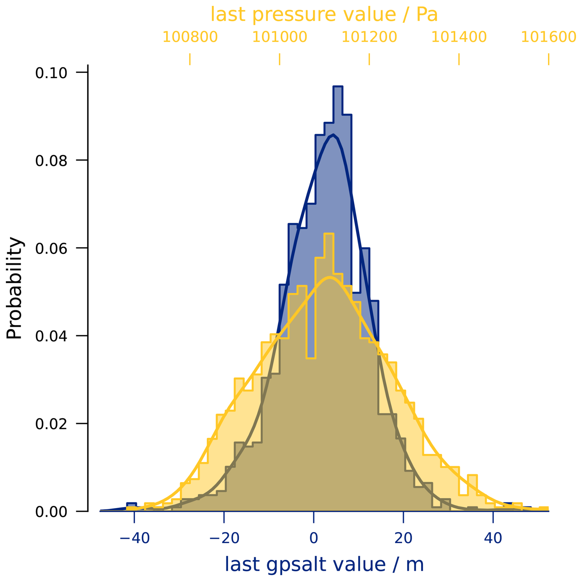
Figure 4Distribution of surface pressure and gpsalt values from all sondes (xrange alt: 100 m, xrange p: 10 hPa).
For sondes that do not have a valid gpsalt profile, i.e. if the gps-valid QC failed, the alt variable is used for the altitude if a valid surface-p measurement was taken. In addition, if the gpsalt profile is incomplete, i.e. if the near-surface-count or the profile-extent QC tests failed for u (meaning there was poor GPS signal), the alt variable is used for the altitude if
-
the QC that was failed for u was passed for p and
-
a valid surface-p measurement was taken.
The first condition ensures that an incomplete gpsalt profile is not replaced by an equally incomplete alt profile. The second condition is required because the alt calculation needs a reference height, and the ASPEN software used for generating Level 1 assumes that the last measured pressure is the surface pressure for that purpose. Although we can never say with 100 % certainty that a sonde sent data until its splash, we assume that it was close enough if the sfc-physics QC was passed for p.
The chosen altitude dimension for each sonde is renamed to altitude in Level 3 to indicate that it is a new variable, and an ancillary variable altitude_source is added to the QC dataset, which contains the name of the altitude variable from Level 2 that is used as the altitude in Level 3 for each sonde. For five sondes on HALO-20240827a, neither gpsalt nor alt provides a valid altitude. These sondes are dropped between Level 2 and 3.
3.3.2 Variables in Level 3
In addition to the Level 2 variables, Level 3 contains θ, q, integrated water vapor (IWV), wind direction and wind speed. Vertical velocity w of individual sondes as estimated by ASPEN, is removed between Level 2 and Level 3. The specific humidity q is calculated from RH and T using the saturation vapor pressure from Hardy (1998), because the same formulation is used by Vaisala for the calibration of the sondes:
with the coefficients given in Table 2

The integrated water vapor (IWV) is only added for sondes that have a GOOD quality control flag for RH, p, and T measurements and set to NaN otherwise to ensure an adequate representation of the actual IWV. We use
The time coordinate from Level 2 is also interpolated and stored in an interpolated_time variable. This time coordinate, as it is interpolated, is no longer useful to calculate fall speeds. These should be computed from the Level 2 data if necessary.
3.4 Level 4: Circle Variables
Level 4 (Gloeckner et al., 2026f) of the BEACH datasets contains the mesoscale divergence (𝒟), vorticity, vertical velocities, and pressure velocity (ω), all of which were derived from circles. Circles usually had a radius of either ca 133 km and a duration of one hour, or of about 70 km and a duration of 40 min (see Sect. 2).
The BEACH Level 3 sonde dataset is grouped into individual circles according to the flight segmentation. The segmentation provides the circle times, latitudes, longitudes, and radii. A sonde belongs to a given circle if it was dropped between the circle's start and end time. In addition sondes dropped inside the circle area and within 20 min from the circle start or end are tagged as extra_sondes in the flight segmentation for that circle and are also included.
We apply the linear regression method described in Bony and Stevens (2019) in order to obtain the gradient terms and the mean profiles. From these, we compute divergence, vorticity, vertical velocity, and ω. Before applying the regression, vertical gaps in the Level 3 profiles are interpolated using the Akima method (Akima, 1970). The details of the interpolation, the regression, the circle products, and corresponding errors are described in this section.
3.4.1 Circle Fit
The regression method is applied as described in Bony and Stevens (2019) and George et al. (2021): The solution to the equation
where δx and δy are the eastward and northward distances to the circle center, is found by solving the least square problem
where , and for a circle with k sondes. This system can be solved with the Moore-Penrose pseudo-inverse to derive ϕ0, which is the circle mean, , which is the linear variation in the eastward direction, and , which is the linear variation in the northward direction (George et al., 2021). Each of these variables are given at every altitude that contains values from six or more sondes, after gaps are vertically interpolated. The details for the interpolation are discussed in Sect. 3.4.3.
3.4.2 Circle Products
The above mentioned components for u and v on the circle scale can be used to derive the area-averaged horizontal divergence, 𝒟, and vorticity ζ:
and the vertical velocity w, and the pressure velocity ω given as
3.4.3 Vertical gap interpolation of sonde profiles
Although 12 to 15 sondes were dropped in a typical circle, not all circles contain full measurements from 12 or more sondes (see Sect. 2.2). This raises the questions of (1) how to handle sondes without valid data and (2) what to do with sondes that provide partial data, but don't pass all quality control checks (Sect. 3.2). Sondes that do not provide valid data, for example due to a launch detection failure, were ignored. Following an error analysis by Bony and Stevens (2019), the errors incurred should be tolerable if six ore more sondes contribute to the products. In the case of measurements from fewer than six sondes circle products are not calculated. That is only the case for the ATR-coordinated circle on HALO-20240827a and the first circle on HALO-20240914a, due to a full dropsonde system failure on both flights.
Apart from sondes that do not contain data at all, there are many sondes with vertical gaps in the measurements. The profile sparsity is largest for u and v, which are used in the divergence calculation (Fig. 3, left). Since the meteorological situation is very variable in the ITCZ (the domain of BEACH), dismissing information that could be interpolated with confidence might lead to larger errors in the divergence, vorticity, vertical velocity, and ω estimation than would arise from simply interpolating gaps. We tested this train of thought using circles with at least 12 sondes with GOOD u, v and p measurements, as defined in Sect. 3.2. For one of those circles with n sondes, ω was calculated times: (1) using all available data and no vertical interpolation (no int), (2) using all data and vertically interpolating gaps with the Akima method (int), (3) once for every sonde assuming that the sonde has an artificial gap at 500 m with interpolation (gap int), and (4) once for every sonde assuming that the sonde has an artificial gap at 500 m without interpolation (gap no int). For interpolation we use the Akima splines (Akima, 1970), which are similar to a cubic-spline interpolation but less prone to overshooting. In the boundary layer missing values are extrapolated by assuming constant u, v, and θ, and linear extrapolation for log (p) and RH.
Figure 5 shows the vertical sum of the differences between no int and gap no int on the x-axis and the vertical sum of the differences between int and gap int on the y-axis for different gap sizes in the columns. The difference to the full calculation becomes larger for larger gap sizes (left to right), which is not surprising as more information about the actual situation is missing. For small gaps, the vertical mean absolute error without interpolation ( hPa h−1) is roughly two orders of magnitude larger than when an interpolation is applied ( hPa h−1). For intermediate gaps, there are some calculations with a noticeably larger error with an interpolation, but overall the mean of absolute errors ( hPa h−1) is approximately quartered as compared to no interpolation ( hPa h−1). For large gaps, it does not make a difference whether an interpolation is applied ( hPa h−1), which again is anticipated as we do not expect the measurements to be informative over such large gaps. Based on those results, we interpolate gaps up to 1500 m.
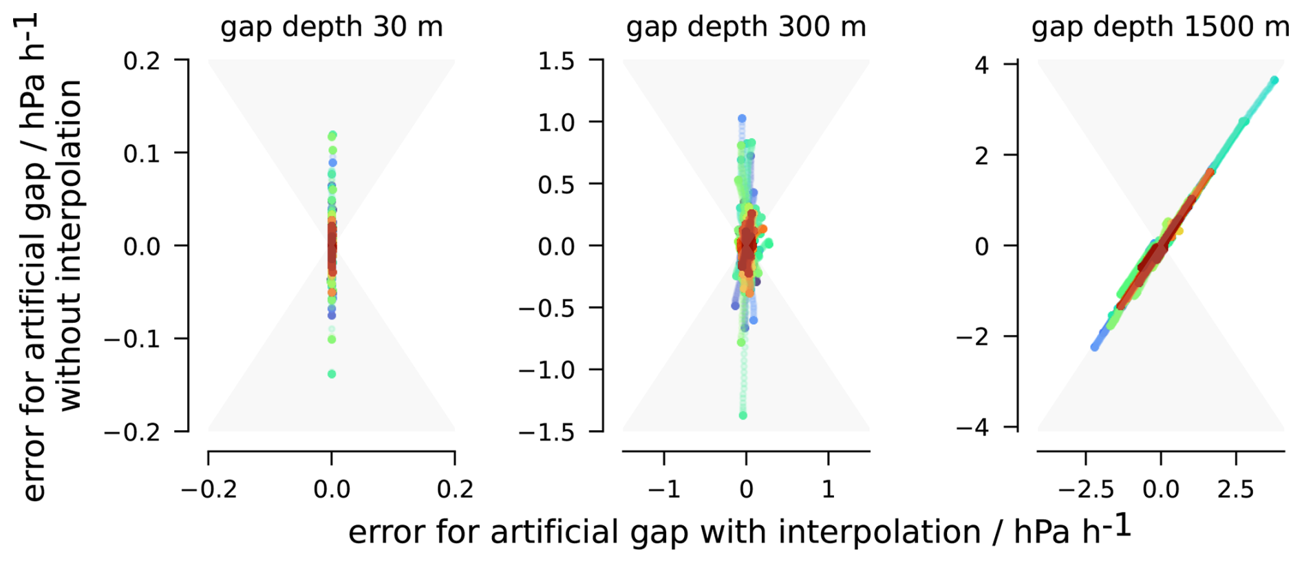
Figure 5Difference to full omega calculation for artificially introduced vertical gaps of 30, 300, and 1500 m depth at 500 m altitude for circles with 12 or more sondes with GOOD u, v and p measurements. Differences using the interpolation method are on the x-axis, differences without interpolation on the y-axis. Each color represents a circle and each large dot the median over altitude for one sonde. The grey area illustrates where the interpolation leads to better results than no interpolation. Be aware that the axes do not have the same scale in the different columns.
3.4.4 Error measures
We calculated the regression standard error for the circle products as described in Bony and Stevens (2019). In addition, we tested the sensitivity of ω to the removal of an individual sonde in the circle. To do so, we removed each sonde from its circle and calculated the circle products again while ignoring this sonde. The difference to the value calculated using all profiles in the circle is stored in a variable omega_remove_sonde_qc.
Figure 6 (middle and right) shows the ω of seven arbitrary circles with the two different error measures in shading. In the middle panel we show the regression standard error and on the right we show the span between the minimum and maximum value if a sonde is removed. The sonde-removal calculation was also done for 𝒟, vorticity, and vertical velocity. The results are stored in the variables *_remove_sonde_qc.
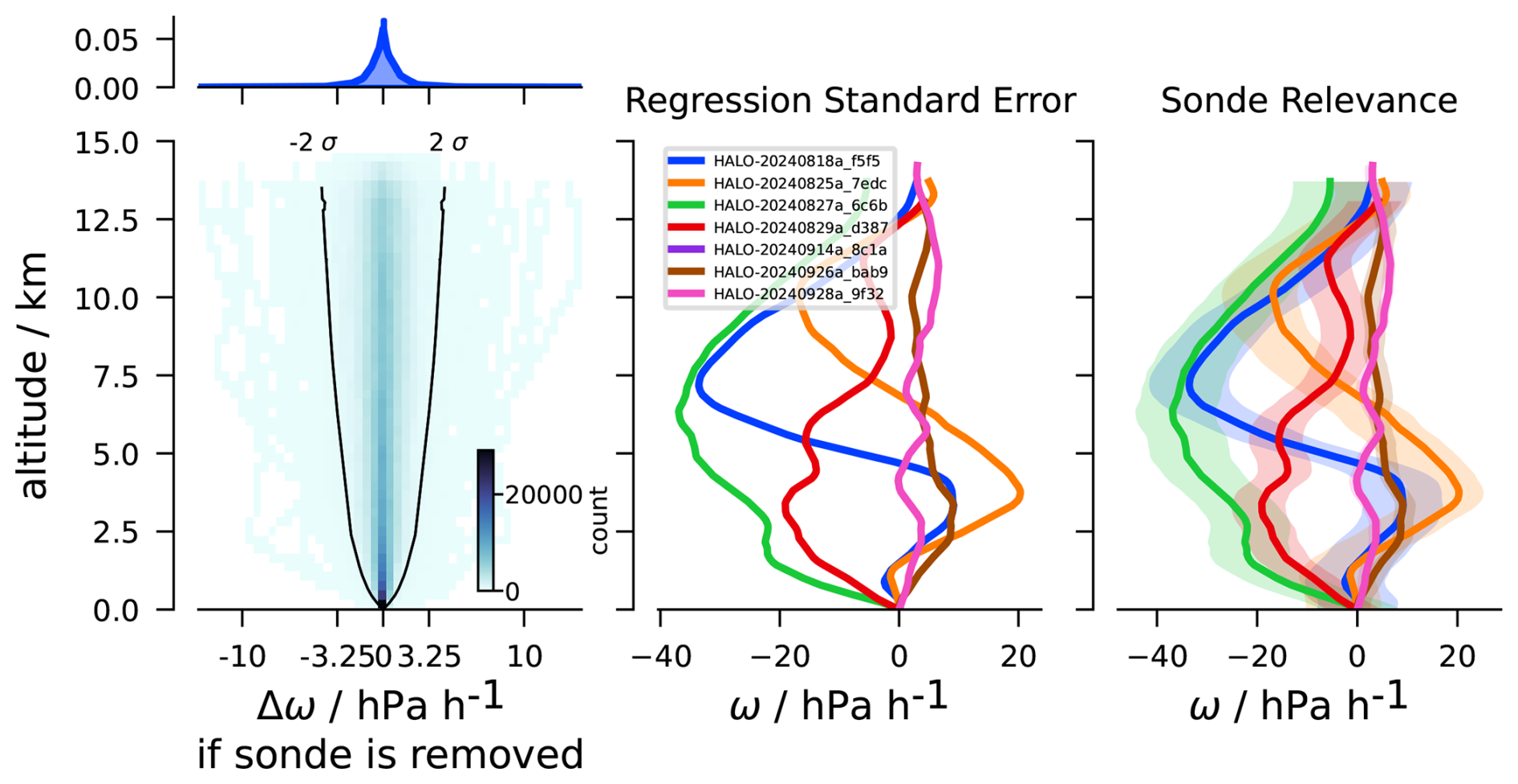
Figure 6Histogram of the error ϵω, with profiles from all circles where any sonde is removed from its circle in lower panel (left). Regression standard error for seven arbitrary circles (middle). Range of minimum and maximum estimate if a sonde is removed from circle calculation for the same circles (right).
Although the regression standard error is small (≈6 % in the mean), individual sondes can have a large impact on the calculated omega. Figure 6 (left) shows a histogram of the errors that emerge if individual sondes are removed. It illustrates that the relevance of the sondes increases with height, which is a direct implication of the integration of divergence, and that the overall mean ω is reliable up to 3.1 hPa h−1 (2σ, averaged over altitude). For individual circles the importance of single sondes can be much larger, as indicated by the spread in the histogram. Hence, if studying individual circles it is useful to check the relevance of individual sondes before interpreting omega values. Encouragingly, the sign of ω does not change in roughly 90 % of the points (and if so then for values of ω≈0).
3.4.5 Variables in Level 4
The Level 4 dataset contains the interpolated profiles of all sondes that belong to a circle as well as all circle products. Consequentially, in addition to the altitude dimension, it has a circle and a sonde dimension, but each variable is only dependent on one of them. To connect both, the dataset has a contiguous ragged array representation following the respective CF-conventions. It contains a sondes_per_circle variable which gives the number of sondes contained in each circle. As long as both dimensions remain sorted by circle_time and launch_time respectively, this structure allows to select all sondes from a circle.
For the sondes, only the sonde_qc information is kept. The interpolated time is also not in the Level 4 dataset. For each of p, RH, q, T, θ, u, and v the fit as described in Sect. 3.4.1 leads to the new variables mean_*, d*dx and d*dy on the circle level. The necessary x and y variables are also saved in the Level 4 dataset.
In addition to divergence, vorticity, ω, and vertical velocity, the standard errors and the remove-sonde-errors are added for those variables. The latter have sonde instead of circle as a dimension, because they are the difference in specific variables, if one sonde is removed.
3.5 Main differences between BEACH and JOANNE
Although the processing has been adapted from the JOANNE processing, which has been conducted on the EUREC4A dropsonde data (George et al., 2021), many steps in the processing have changed.
From Level 2 onward, BEACH does not use the serial ID from the manufacturer as a unique reference to a sonde since there can be multiple files containing the same serial ID (Sect. 2.2). Instead, a hash derived from the first line in the D-file (including launch-time and manufacturer serial-ID) was used.
For the calculation of Level 2, the QC tests have been rearranged: The profile-fullness/sat-test in JOANNE is renamed to profile sparsity and the fraction of missing values as compared to a hypothetical perfect sonde measurement is calculated instead of the fraction of measured values. JOANNE's surface-test has been split into a surface count (near-surface-count) and a surface physics test (sfc-physics). They are both present in JOANNE but combined to the low-altitude-measurement-test/low-test. An additional test that checks the profile-extent was introduced to flag sondes with incomplete profiles, e.g. if the parachute opened very late, and which are problematic when comparing integrated quantities such as integrated water vapor.
Contrarily to JOANNE, sondes that did not pass the tests were not discarded from the dataset, but flagged in the Level 2 and Level 3 datasets. Additionally, a var_qc variable is introduced that contains the QC information in binary format for all variables. Most of those changes have little impact on the overall QC flag, but were introduced to account for edge cases that occurred during PERCUSION and are not covered by the JOANNE QC framework.
During PERCUSION, all sondes were reconditioned on the morning of the flight that they were dropped. As a consequence there is no dry bias correction (as described in George et al., 2021) and the humidity measurements are consistent across data levels.
In BEACH Level 3, the altitude derived from GPS measurements, gpsalt, is used as the default height coordinate instead of pressure altitude alt. However, if no gpsalt values were present or the alt measurements were better, the latter is used. In JOANNE, q and θ are binned to a 10 m grid, while we chose to interpolate to the same grid. The decision to bin was made as to not have values that are not measured in the dataset. This approach was changed, because binning instead of interpolating introduces an error in height of up to 5 m per 10 m bin. Although irrelevant for most applications, it creates an error of a couple of centimeters in the hydrostatic equation that adds up over the depth of the troposphere and is avoided by interpolating. To still maintain consistent RH and q values, BEACH interpolates in RH instead of q, because the former is more linear.
While JOANNE linearly interpolates gaps of up to 50 m in altitude, BEACH Level 3 does not include any gap interpolation larger than 5 m in Level 3. It does however use the Akima-splines interpolation on gaps in the measurements before the circle fits, assumes constant u, v, and θ, and linear RH and log (p) in the lowest 300 m if there are no measurements for Level 4. For convenience, those interpolated profiles are contained in BEACH's Level 4. BEACH also uses sondes that did not pass all QC tests for the Level 4 calculation if the QC of used variables were passed, while JOANNE only uses sondes that passed every QC test.
JOANNE and BEACH use the same formula for vertical velocity w, but BEACH uses the integration over divergence in p for the vertical pressure velocity ω, while JOANNE uses
Calculating w and ω independently comes at the cost that they cannot be easily transformed anymore, but it calculates each variable relative to its altitude coordinate, and hence is more physically accurate. For BEACH, the sonde relevance variables were calculated in addition to the regression standard error.
The dropsondes' surface wind and integrated water vapor measurements give an indication of the conditions spanned by the BEACH data. The moist tropics are mostly defined by an integrated water vapor above 48 mm (Mapes et al., 2018), with a peak near the southern edge of the ITCZ (Windmiller and Stevens, 2024). The integrated water vapor (Fig. 8) confirms that most measurements have been taken within the moist tropics, especially in the East, oftentimes with an IWV much greater than 48 mm.
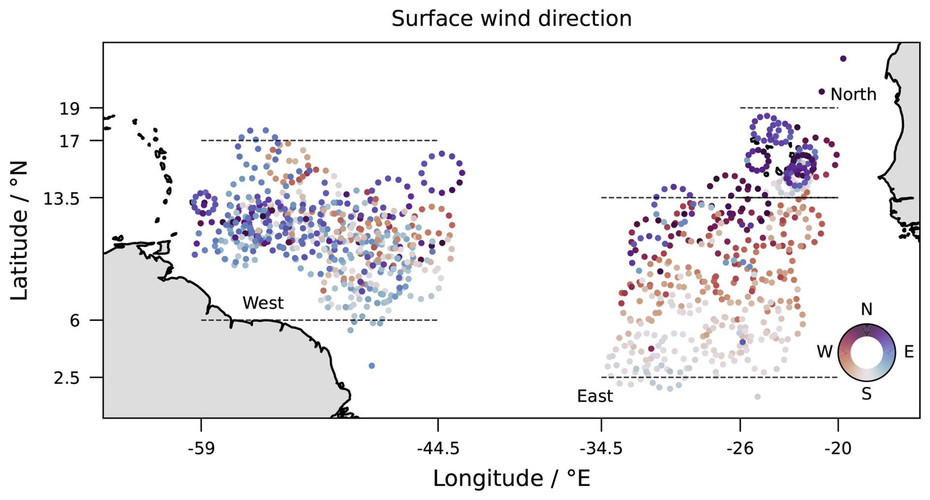
Figure 7Mean wind direction in the lowest 50 m for all sondes. Level 3 data is used for this plot.
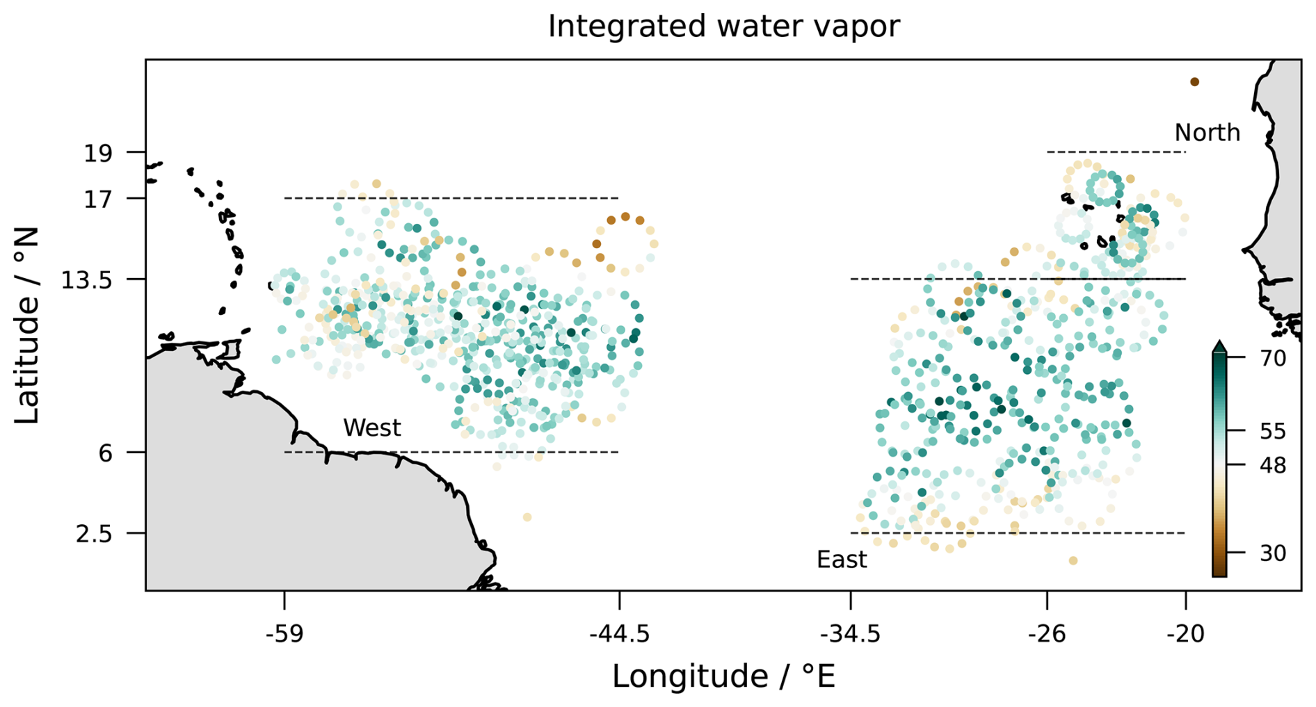
Figure 8IWV of all sondes. Colorbar is centered at 48 mm. Level 3 data is used for this plot.
Since the ITCZ is marked by strong convergence at the surface, we expect the surface wind direction to change at the edge(s) of the ITCZ. Figure 7 shows the surface wind direction of all sondes. Especially in the East the southerlies turn westward as they cross the equator to form the monsoon trough (Flohn, 1951; Praturi and Stevens, 2026). This indicates that most of the dropsondes sampled the breadth of the ITCZ by measure of surface wind direction as well as IWV. Sometimes the ITCZ is distinguished from the monsoon trough through its absence of westerlies, a distinction we do not adopt in this paper.
In the West, neither the wind nor the integrated water vapor field follow the clear structure that is apparent in the East, consistent with the ITCZ being less well defined there (Stevens et al., 2026, Fig. 6).
The vertical profile of the wind shows weak baroclinicity (Fig. 9), where the zonal wind changes sign above 10 km, with the predominant westerlies at the surface transform into strong easterlies higher up in the East, while the easterlies in the West become westerlies in the West.
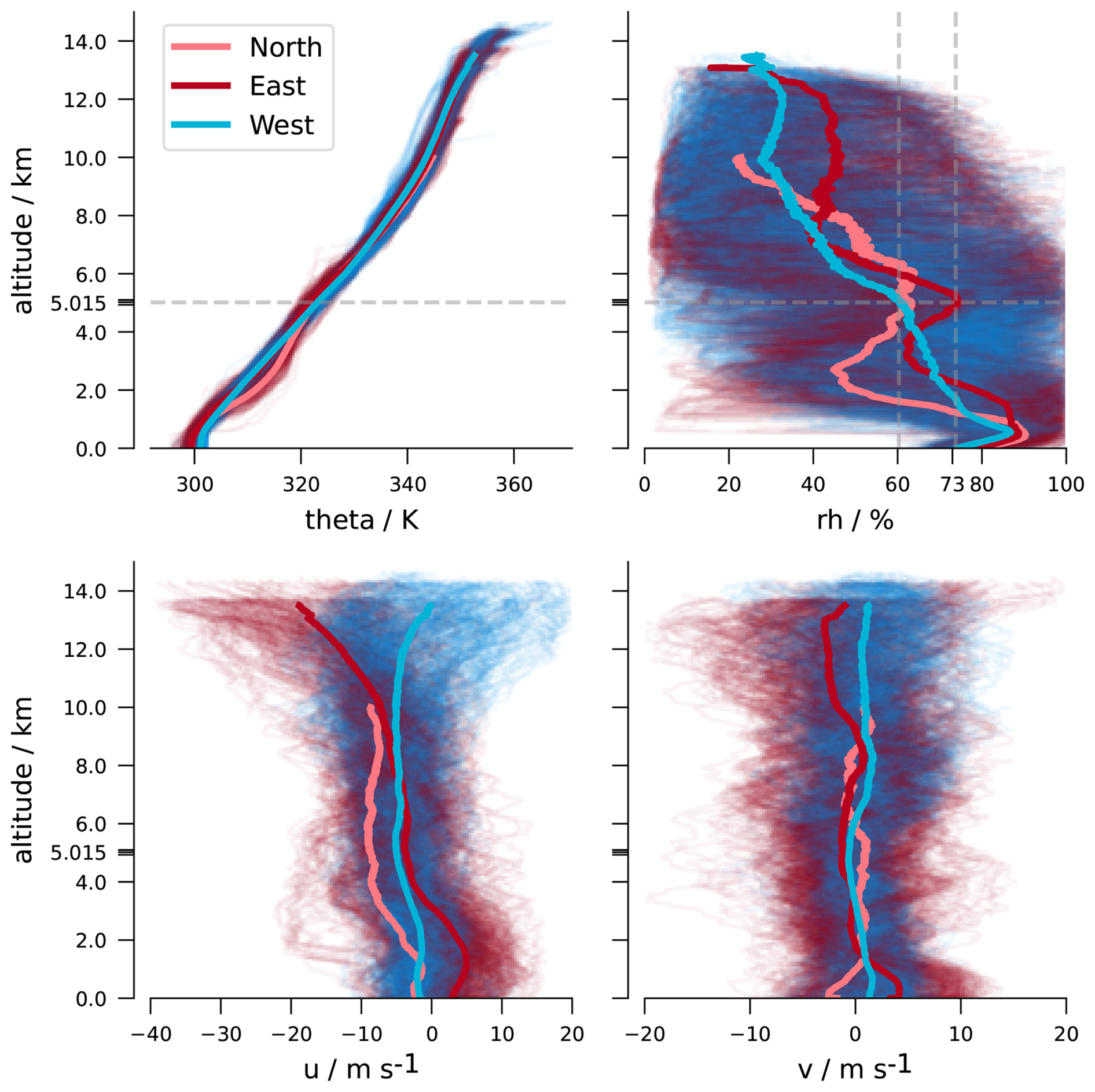
Figure 9Profiles of individual sondes from BEACH Level 3 for θ, RH, u and v from the East region (dark red), West region (blue), and North region (light red). Means are plotted with thick lines while the thin lines correspond to individual profiles (East of −40° E in red and West of −40° E in blue). The gray horizontal lines mark the mean freezing level and the lower relative humidity peak respectively. BEACH Level 3 data is used for this plot.
The larger spread in the near surface wind component v in the East is further evidence for the larger variety of conditions that were sampled there. In the North region, easterlies dominate the whole column, indicating that those sondes were mostly dropped in the trade wind region.
Although it is generally moist everywhere, the relative humidity profiles vary considerably. The mean profile in the East has two distinct peaks at the top of the boundary layer, and near the freezing level and a minimum in between. This structure fits to the trimodal characteristic of tropical convection (Johnson et al., 1999) and might be of interest because reanalyses and satellite observations struggle to represent the elevated moist layers in the mid-troposphere (Prange et al., 2023). This feature is even more pronounced in the North, which might be indicative of a role for dry Saharian air on this region, especially since the winds are predominantly north-easterlies babove 2000 m. In the West, the mean profile shows less evidence of a freezing level maximum, but the troposphere below the 0° isotherm is moister than the troposphere aloft. Note that the humidity profiles above the freezing level rarely reach 100 % but might still be saturated, especially at higher altitudes, as relative humidity is calculated with respect to water instead of ice.
Measurements coordinated with the SAFIRE ATR-42 were in the North region. Although the mean conditions there indicate the trade wind region, some circles as well as a bimodal IWV distribution (see Figs. B1 and B2 in the Appendix) point to several interesting cases in or at the edge of the ITCZ.
Mesoscale vertical air motion in the East, as shown in Fig. 10, supports the idea of the ITCZ being a region of mean ascent with convergence below ≈ 2000 m and divergence above 10 000 m. The West Atlantic shows mean surface divergence in the lower-troposphere similar to the divergence profile from the JOANNE data measured during the EUREC4A campaign, which sampled the winter trades in 2020 (yellow). However, whereas omega in JOANNE indicates subsidence through a deep layer, the mean omega of the Western measurements in BEACH shows rising air motion above ≈ 3000 m. The switch in the direction of vertical air motion however is caused by strong updrafts at these levels prevaling in some circles. Considering the median vertical velocity instead of the mean shows predominant subsidence in the West Atlantic above 3000 m as well. The mean in the East Atlantic is similarly influenced by deep convective events, but the median still shows upward air motion in the whole column.
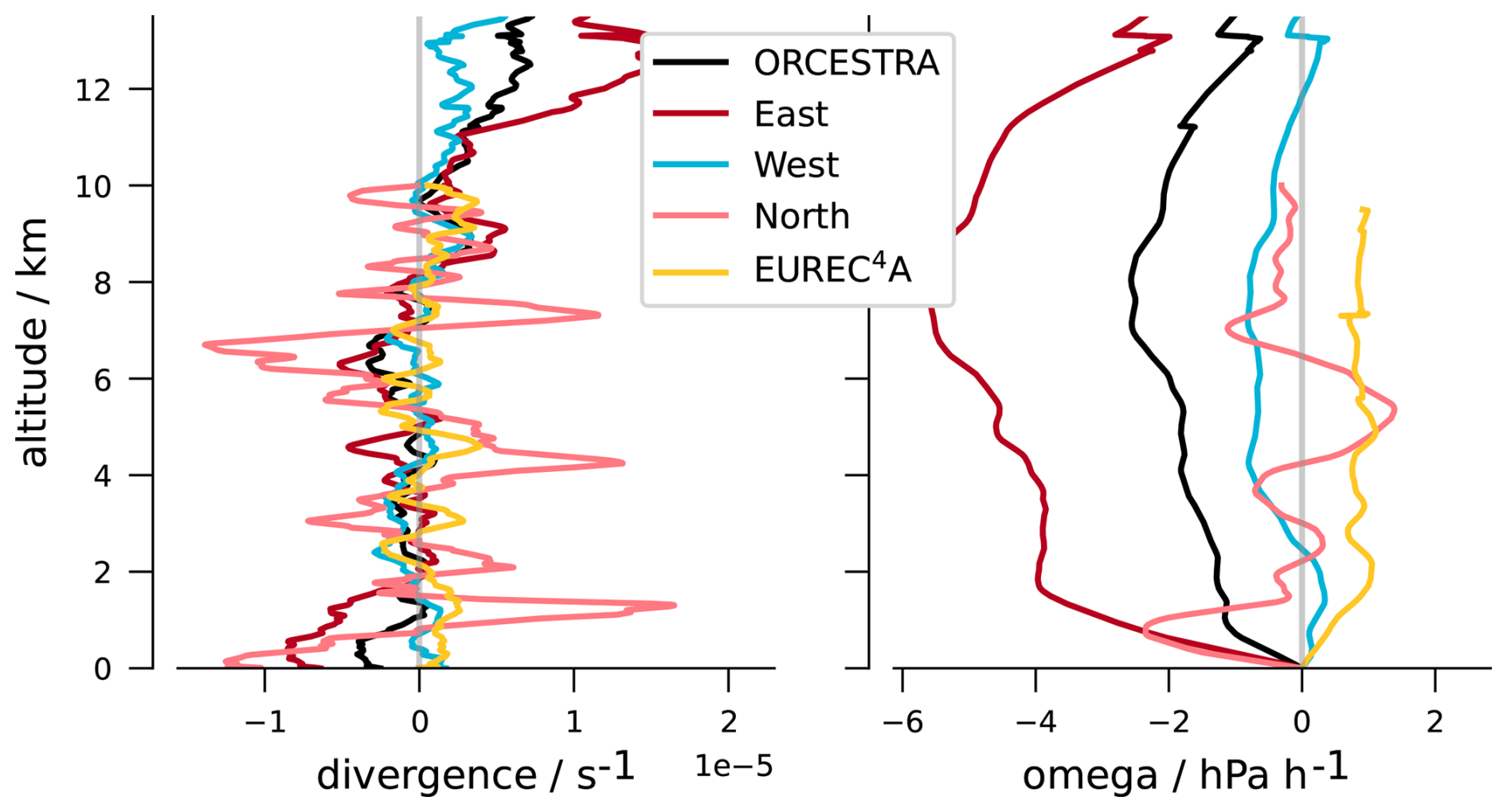
Figure 10Average divergence (left) and omega (right) for the full campaign, as well as split into East and West Atlantic. The average profiles from the JOANNE dataset showing typical characteristics for the winter trades in the Western Atlantic are added for comparison. BEACH Level 4 data is used for this plot.
The East–West difference in mesoscale divergence is shown in more detail in Fig. 11 for all circles in the BEACH dataset. Each column is a circle and flights are separated by black vertical lines with circles and flights being sorted in time from left to right (similar to George et al., 2023, Fig. 1). The transfer from sampling the East Atlantic to the West Atlantic on 6 September is marked at the top. Most obvious are the stronger convergence and divergence patterns in the East (stronger red and blue colors) compared to less strong patterns in the West except for the flight on 24 September.
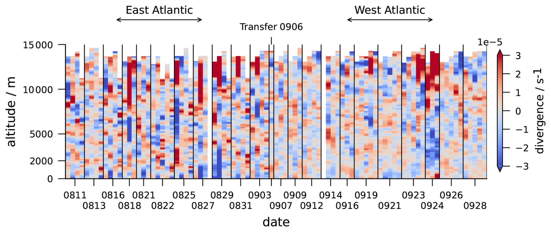
Figure 11Divergence for all circles during the campaign. Flights are separated by black lines. The transfer between East and West is marked at the top. Circles are ordered in time. Level 4 data is used for this plot.
The PERCUSION and MAESTRO aircraft campaigns took place in August and September 2024 in the tropical Atlantic as part of ORCESTRA. A main focus of ORCESTRA was the influence of convective and mesoscale circulation systems on the mean structure of the ITCZ. As part of this effort, 1191 sondes were dropped from the research aircraft HALO. This paper presents the data from these sondes in the form of the BEACH datasets.
The BEACH datasets contain four levels of processing of the raw data (Level 0), as schematically depicted in Fig. 2. This leads to the following data levels: ASPEN quality controlled data (Level 1); custom quality controlled data (Level 2); a combined dataset including all sondes that have at least partially valid data (Level 3); and a dataset containing divergence and vertical velocity on the mesoscale for all circles with sufficient valid sonde measurements (Level 4). All datasets are openly available on IPFS (Stevens et al., 2026). The general hierarchy of the levels and most parts of the processing were adapted from the EUREC4A dropsonde processing (George et al., 2021).
The BEACH dropsonde data confirms that the PERCUSION flight tracks span the meridional extent of the ITCZ, with measurements within as well as at the edges as defined by the surface wind field and integrated water vapor (Figs. 7, 8). It also samples zonal variations within the ITCZ. While the ITCZ is clearly outlined in both the surface wind direction and IWV in the East, in the West it is less structured. Another difference is that in the East there are two distinct peaks in the mean relative humidity – around the freezing level and above the subcloud layer. In the West, there is no distinct peak in RH at the freezing level. In the wind profiles, known dynamical features such as surface westerlies within the equatorial trough are captured as well as a weak imprint of an Atlantic Walker cell, and the African Easterly Jet.
A core objective of the flight strategy was the derivation of mesoscale divergence and vertical velocities from sondes dropped on circular flight patterns. We succeeded in processing 87 circles from all flights that show on average upward motion with stronger updrafts in the East compared to the West Atlantic. Furthermore, in the lowest 2000 m the vertical velocity profile in the West is closer to the JOANNE measurements from the wintertime trades compared to the measurements from the summertime East Atlantic, leaving much room for further analysis.
All datasets in the hierarchy of BEACH are made available via https://ipfs.tech (last access: 18 June 2026) and have a landing page in the ORCESTRA-browser: https://browser.orcestra-campaign.org/ (last access: 18 June 2026)
The respective DOIs are
-
L0: https://doi.org/10.82246/bafybeif4 (Gloeckner et al., 2026a)
-
L1: https://doi.org/10.82246/bafybeieqq (Gloeckner et al., 2026b)
-
L2: https://doi.org/10.82246/bafybeifi5 (Gloeckner et al., 2026c)
-
L3: https://doi.org/10.82246/bafybeiczb (Gloeckner et al., 2026d)
-
L3qc: https://doi.org/10.82246/bafybeidyt (Gloeckner et al., 2026e)
-
L4: https://doi.org/10.82246/bafybeibge (Gloeckner et al., 2026f)
Further information on the ORCESTRA data policy and concept can be found in the ORCESTRA overview paper (Stevens et al., 2026) and on the ORCESTRA campaign website (https://orcestra-campaign.org/data.html, last access: 18 June 2026). The dropsonde processing software generating the various data levels is available on GitHub in the pydropsonde repository as well as a Python package called pydropsonde via the Python Package Index (PyPI) (https://github.com/atmdrops/pydropsonde, last access: 18 June 2026; https://doi.org/10.5281/zenodo.20745099, George et al., 2026). For the processing and plots presented in this paper version 0.5.5 was used which includes the initial processing with ASPEN v4.0.4. The ASPEN software is hosted in a docker image on GitHub (https://github.com/atmdrops/aspenqc, last access: 18 June 2026; https://doi.org/10.5281/zenodo.20745087, Mieslinger et al., 2026), making it independent from the operating system. The repository includes a Dockerfile and the respective GitHub workflows needed to generate the image and push it to the GitHub container registry. It can be used via it's name: https://ghcr.io/atmdrops/aspenqc (last access: 18 June 2026). The configuration file for running pydropsonde on the ORCESTRA dropsondes as well as all analysis scripts generating plots and tables for this paper are stored on GitHub in the orcestra-campaign-dropsondes repository (https://github.com/orcestra-campaign/dropsondes, last access: 18 June 2026; https://doi.org/10.5281/zenodo.20749911, Gloeckner et al., 2026g).
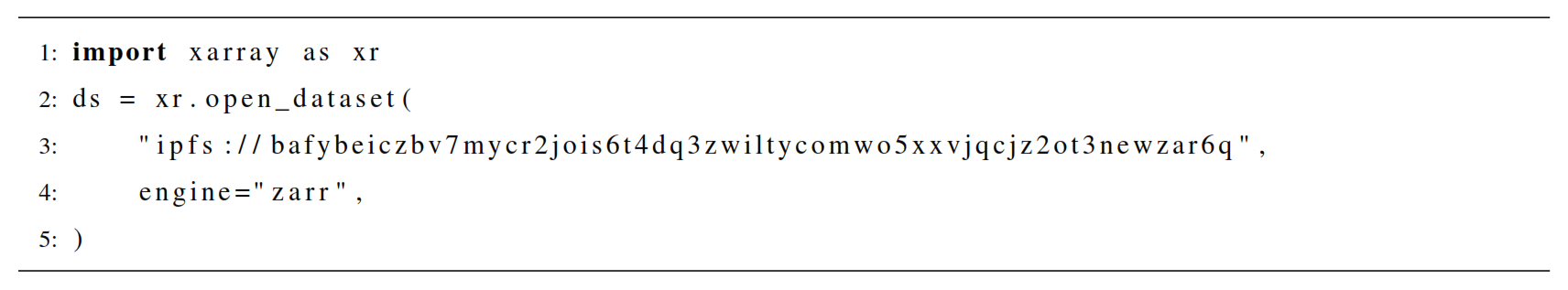
The BEACH datasets are stored such that they can be easily accessed with a few lines of code. For example, one can access the Level 3 BEACH dataset directly using Python. This requires a working IPFS Gateway and the ipfsspec package to be installed.
| ASPEN | Atmospheric Sounding Processing ENvironment |
|---|---|
| AVAPS | Airborne Vertical Atmospheric Profiling System |
| BAHAMAS | Basic Halo Measurement and Sensor System |
| BEACH | Barbados and Eastern Atlantic Combined High-altitude dropsonde datasets |
| EarthCARE | Earth Clouds, Aerosols and Radiation Explorer |
| EUREC4A | Elucidating the role of clouds-circulation coupling in climate 2020 |
| GATE | GARP Atlantic Tropical Experiment 1974 |
| GARP | Global Atmospheric Research Project |
| GPS | Global Positioning System |
| HALO | High-Altitude and LOng range research aircraft |
| HALO-(AC)3 | Arctic Air Mass Transformations During Warm Air Intrusions and Marine Cold Air Outbreaks 2021 |
| ICON | The ICOsahedral Non-hydrostatic model |
| IFS | Integrated Forcasting Model (ECMWF) |
| INMG | Instituto Nacional de Meteorologia e Geofísica (Cabo Verde) |
| IPFS | Inter Planetary File System |
| ITCZ | InterTropical Convergence Zone |
| JOANNE | Joint dropsonde Observations of the Atmosphere in tropical North-atlaNtic meso-scale Environments |
| MAESTRO | Mesoscale organisation of tropical convection subcampaign of ORCESTRA |
| NARVAL2 | Next-generation Aircraft Remote-sensing for VALidation studies (2) 2016 |
| NCAR | National Center of Atmospheric Research (US) |
| netCDF | Network Common Data Format |
| ORCESTRA | Organized Convection and EarthCARE Studies over the Tropical Atlantic 2024 |
| OTREC | Organisation of Tropical East Pacific Convection 2019 |
| PERCUSION | Persistent EarthCARE underflight studies of the ITCZ and organized convection subcampaign of |
| ORCESTRA | |
| PTU sensor | Pressure Temperature and hUmidity sensor |
| RAPSODI | Radiosonde Atmospheric Profiles from Ship and island platforms during ORCESTRA, |
| collected to Decipher the ITCZ | |
| SAFIRE ATR-42 | Service des Avions Français Instrumentés pour la Recherche en Environnemen (Avions de |
| Transport Régional 42) |
During the ORCESTRA campaign, 10 circles were flown in coordination with the SAFIRE ATR-42. Table B1 shows the segment IDs of those circles as well as the SAFIRE ATR-42 flight that was closest in time, and the number of sondes in Level 3 and Level 4 for those circles. Apart from one circle on HALO-20240827, where the system shut down (see Sect. 2.2), all SAFIRE ATR-42-coordinated circles have 10 or more sondes.
Figure B1 is similar to Fig. 10, but including the ATR divergence and omega estimates. Contrarily to the figure in the main text, here the mean omega and divergence for the East Atlantic does not include the ATR values. This illustrates that the ATR circles were mostly flown in a different environment than the larger circles. Thin yellow lines in the plot are individual ATR circles and demonstrate the spread in the measurements.
Figure B2 further shows the distribution in integrated water vapor and how it differs between SAFIRE ATR-42 coordinated sondes and the others. Again, the curve for the East Atlantic excludes SAFIRE ATR-42 coordinated measurements. All distributions have a peak close to 60 mm IWV, which is well above the 48 mm threshold assumed for the ITCZ in the long term mean. The distribution of ATR dropsondes has a distinguished second peak at lower IWV values (≈ 48 mm), indicating that the majority of those sondes were dropped at the edge or outside of the ITCZ.
Table B1PERCUSION ATR coordination statistics showing the closest ATR flight to each atr-coordinated HALO circle and the number of sondes in Level 3 and Level 4 for those circles.
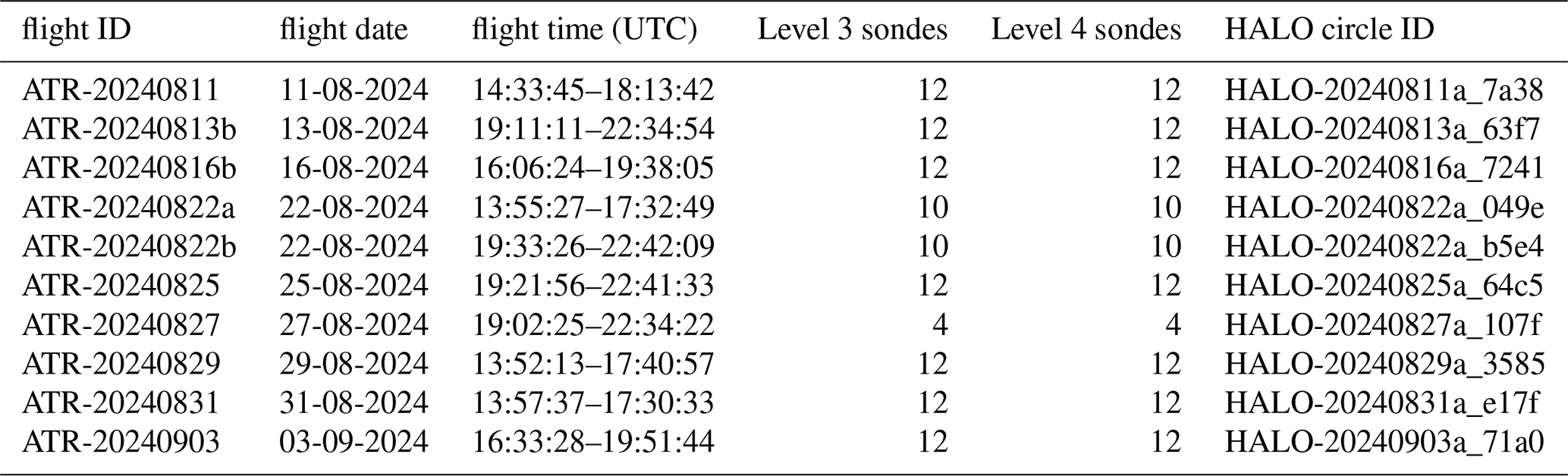
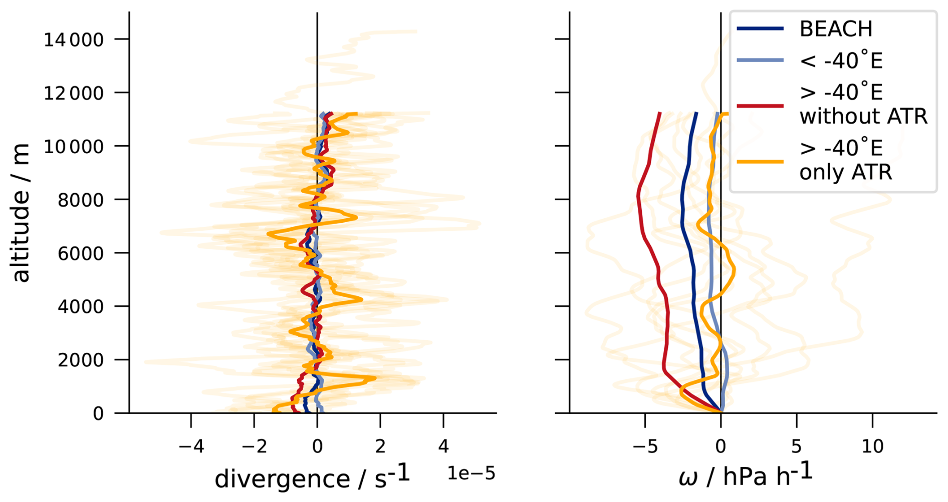
Figure B1Divergence for all circles during PERCUSION (dark blue), for the West Atlantic (light blue), compared to only circles in the East Atlantic (without ATR – red) and only the circles flown in coordination with SAFIRE ATR-42 (yellow).
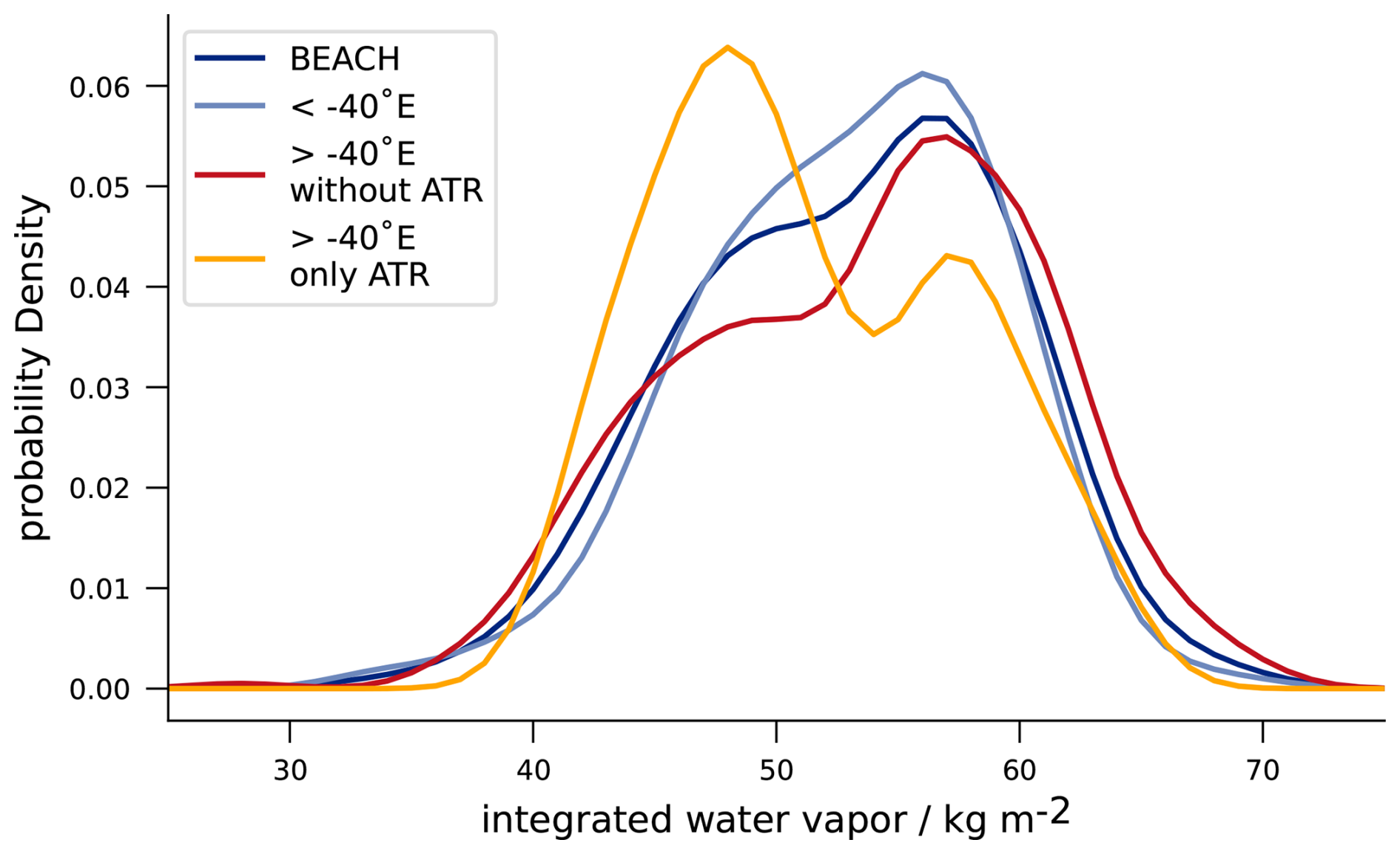
Figure B2Normalized probability density of integrated water vapor for the full PERCUSION campaign (dark blue), for the West Atlantic (light blue), from the Eastern Atlantic (without ATR – red), and only from measurements in coordination with the SAFIRE ATR-42 (yellow).
SB, JW, and BS conceptionalized the measurements and developed the flight and drop strategy for PERCUSION and the coordination with MAESTRO. HMG, TM, and NRB dropped the majority of sondes that form the BEACH datasets. GG initialized the halodrops repo and HMG, TM, NRB, GG, LK, and TK developed it into the pydropsonde package. HMG and TM prepared the data overview (Sect. 4) and figures with input from all other authors. HMG prepared the paper draft with contributions by all other authors.
The contact author has declared that none of the authors has any competing interests.
Publisher's note: Copernicus Publications remains neutral with regard to jurisdictional claims made in the text, published maps, institutional affiliations, or any other geographical representation in this paper. The authors bear the ultimate responsibility for providing appropriate place names. Views expressed in the text are those of the authors and do not necessarily reflect the views of the publisher.
We thank Friedhelm Jansen and Lutz Hirsch that they handled the logistics for the sondes; and Felix Ament who provided an additional 50 sondes he found under his desk on Barbados.
We appreciate the help Holger Vömel offered regarding our problematic sondes during the processing.
We are grateful to James Ruppert and Allison Wing, because they pointed out a bug in the integrated water vapor calculation in an earlier version of the data, and Basile Poujol for pointing out an inaccuracy in the vertical pressure velocity calculation in JOANNE.
We further credit Jakob Deutloff, Allison Wing, and Marius Winkler who operated the sonde system for one of the flights, as well as Lutz Hirsch, Elina Plesca, Daniel Rowe, Luca Schmidt, and Yuting Wu who got up early in the morning to recondition the sondes.
We also recognize everyone who helped with the communication during one of the flights: Felix Ament, Romain Fievet, Henning Franke, Silke Gross, Suelly Katiza, Daniel Klocke, Brett McKim, Chelsea Nam, Sebastian Ortega Arango, Elina Plesca, Basile Poujol, Chavez Pope, Divya Praturi, Rene Redler, Marius Rixen, Nicolas Rochetin, Daniel Rowe, Martin Singh, Lea Volkmer, Tristan Vostry, and Manfred Wendisch.
And of course Yuting Wu again, who came up with the name for BEACH.
ORCESTRA was made possible thanks to the support of the Max Planck Society (MPG) and the French National Centre for Scientific Research (CNRS). Additional financial support was provided by the German Research Foundation (DFG) through grant number GPF20-1072; by the Dutch Research Council (NWO); by the US National Science Foundation (NSF) through Award Numbers 2331199, 2331200, and 2331202; by the ESA Earth Observation Envelope Programme (ESA-EOEP) contract No. 4000145240/24/NL/SC; by EU-HORIZON-WIDERA-2021 Grant 101079385 (BRACE-MY) and the European Research Council (ERC) Consolidator Grant 101045273 (STEP-CHANGE). MAESTRO was supported by the ERC through Advanced Grant 101098063 (MAESTRO), with further financial support from ESA (contract no. 281042) and CNES (EMC-Sat). PERCUSION received further financial support from ESA under contract No. 4000145500/24/NL/SC, by the DLR-internal project MABAK (Innovative Methoden zur Analyse und Bewertung von Veränderungen der Atmosphäre und des Klimasystems), by the German National Science Foundation’s (DFG) Priority Program (Schwerpunktprogramm) SPP 1294 “Atmospheric and Earth System Research with HALO – High Altitude and Long Range Research Aircraft” from Horizon Europe programme under Grant Agreement No 101137680 via project CERTAINTY (Cloud-aERosol inTeractions & their impActs IN The earth sYstem), and by the German Federal Ministry of Research, Technology and Space (BMFTR) under the funding code 01LK2202B (WarmWorld). NRB acknowledges support from the ERC starting grant ROTOR (grant no. 101116282). GG acknowledges financial support from HALO DFG SPP 1294 to organize the HALODROPS workshop which kick-started the efforts to develop a dropsonde package that has evolved into the current pydropsonde package.
The article processing charges for this open-access publication were covered by the Max Planck Society.
This paper was edited by Montserrat Costa Surós and reviewed by two anonymous referees.
Aberson, S. D., Zhang, J. A., Zawislak, J., Sellwood, K., Rogers, R., and Cione, J. J.: The NCAR GPS dropwindsonde and its impact on hurricane operations and research, Bull. Am. Meteorol. Soc., 104, E2134–E2154, 2023. a
Akima, H.: A New Method of Interpolation and Smooth Curve Fitting Based on Local Procedures, J. ACM, 17, 589–602, https://doi.org/10.1145/321607.321609, 1970. a, b
AspenDocs 1.0: AspenDocs 1.0, https://ncar.github.io/aspendocs/man_qc.html, last access: 28 May 2025. a
Back, L. and Bretherton, C.: Geographic variability in the export of moist static energy and vertical motion profiles in the tropical Pacific, Geophys. Res. Lett., 33, https://doi.org/10.1029/2006GL026672, 2006. a
Bellamy, J. C.: Objective calculations of divergence, vertical velocity and vorticity, Bull. Am. Meteorol. Soc., 30, 45–49, 1949. a
Bernardez, M. and Back, L.: Integrating thermodynamic and dynamic views on the control of the top-heaviness of convection in the Pacific ITCZ with weak temperature gradient simulations, J. Adv. Model. Earth Syst., 16, e2022MS003455, https://doi.org/10.1029/2022MS003455, 2024. a
Bony, S. and Stevens, B.: Measuring Area-Averaged Vertical Motions with Dropsondes, J. Atmos. Sci., 76, 767–783, https://doi.org/10.1175/JAS-D-18-0141.1, 2019. a, b, c, d, e, f, g
Bony, S., Stevens, B., Ament, F., Bigorre, S., Chazette, P., Crewell, S., Delanoë, J., Emanuel, K., Farrell, D., Flamant, C., Gross, S., Hirsch, L., Karstensen, J., Mayer, B., Nuijens, L., Ruppert, J. H., Jr., Sandu, I., Siebesma, P., Speich, S., Szczap, F., Totems, J., Vogel, R., Wendisch, M., and Wirth, M.: EUREC 4 A: A field campaign to elucidate the couplings between clouds, convection and circulation, Surv. Geophys., 38, 1529–1568, 2017. a
Eaton, B., Gregory, J., Drach, B., Taylor, K., Hankin, S., Caron, J., Signell, R., Bentley, P., Rappa, G., Höck, H., Pamment, A., Juckes, M., Raspaud, M., Horne, R., Blower, J., Whiteaker, T., Blodgett, D., Zender, C., Lee, D., Hassell, D., Snow, A. D., Kölling, T., Allured, D., Jelenak, A., Soerensen, A. M., Gaultier, L., Herlédan, S., Manzano, F., Bärring, L., Barker, C., and Bartholomew, S.: NetCDF Climate and Forecast (CF) Metadata Conventions, Zenodo, https://doi.org/10.5281/zenodo.14275599, 2024. a, b
Ceselski, B. F. and Sapp, L. L.: Objective wind field analysis using line integrals, Mon. Weather Rev., 103, 89–100, 1975. a
Ehrlich, A., Crewell, S., Herber, A., Klingebiel, M., Lüpkes, C., Mech, M., Becker, S., Borrmann, S., Bozem, H., Buschmann, M., Clemen, H.-C., De La Torre Castro, E., Dorff, H., Dupuy, R., Eppers, O., Ewald, F., George, G., Giez, A., Grawe, S., Gourbeyre, C., Hartmann, J., Jäkel, E., Joppe, P., Jourdan, O., Jurányi, Z., Kirbus, B., Lucke, J., Luebke, A. E., Maahn, M., Maherndl, N., Mallaun, C., Mayer, J., Mertes, S., Mioche, G., Moser, M., Müller, H., Pörtge, V., Risse, N., Roberts, G., Rosenburg, S., Röttenbacher, J., Schäfer, M., Schaefer, J., Schäfler, A., Schirmacher, I., Schneider, J., Schnitt, S., Stratmann, F., Tatzelt, C., Voigt, C., Walbröl, A., Weber, A., Wetzel, B., Wirth, M., and Wendisch, M.: A comprehensive in situ and remote sensing data set collected during the HALO-(AC)3 aircraft campaign, Earth Syst. Sci. Data, 17, 1295–1328, https://doi.org/10.5194/essd-17-1295-2025, 2025. a
Flohn, H.: Passatzirkulation und äquatoriale Westwindzone, Arch. Meteorol., Geophys. Bioklimatol., Ser. B, 3, 3–15, 1951. a
Fuchs-Stone, Ž., Raymond, D. J., and Sentić, S.: OTREC2019: Convection over the east Pacific and southwest Caribbean, Geophys. Res. Lett., 47, e2020GL087564, https://doi.org/10.1029/2020GL087564, 2020. a
George, G., Stevens, B., Bony, S., Pincus, R., Fairall, C., Schulz, H., Kölling, T., Kalen, Q. T., Klingebiel, M., Konow, H., Lundry, A., Prange, M., and Radtke, J.: JOANNE: Joint dropsonde Observations of the Atmosphere in tropical North atlaNtic meso-scale Environments, Earth Syst. Sci. Data, 13, 5253–5272, https://doi.org/10.5194/essd-13-5253-2021, 2021. a, b, c, d, e, f, g, h, i, j, k
George, G., Stevens, B., Bony, S., Vogel, R., and Naumann, A. K.: Widespread shallow mesoscale circulations observed in the trades, Nat. Geosci., 16, 584–589, 2023. a
George, G., Gloeckner, H. M., Mieslinger, T., Robbins-Blanch, N., Kluft, L., Kölling, T., and Dorff, H.: atmdrops/pydropsonde: zenodo, Zenodo [code], https://doi.org/10.5281/zenodo.20745099, 2026. a
Gloeckner, H. M., Mieslinger, T., and Robbins-Blanch, N.: BEACH dropsonde dataset (Level 0), https://doi.org/10.82246/bafybeif4n, 2026a. a, b
Gloeckner, H. M., Mieslinger, T., and Robbins-Blanch, N.: BEACH dropsonde dataset (Level 1), https://doi.org/10.82246/bafybeieqq, 2026b. a, b
Gloeckner, H. M., Mieslinger, T., and Robbins-Blanch, N.: BEACH dropsonde dataset (Level 2), https://doi.org/10.82246/bafybeifi5, 2026c. a, b
Gloeckner, H. M., Mieslinger, T., and Robbins-Blanch, N.: BEACH dropsonde dataset (Level 3), https://doi.org/10.82246/bafybeiczb, 2026d. a, b
Gloeckner, H. M., Mieslinger, T., and Robbins-Blanch, N.: BEACH dropsonde dataset (Level 3) QC, https://doi.org/10.82246/bafybeidyt, 2026e. a
Gloeckner, H. M., Mieslinger, T., and Robbins-Blanch, N.: BEACH dropsonde dataset (Level 4), https://doi.org/10.82246/bafybeibge, 2026f. a, b
Gloeckner, H. M., Mieslinger, T., and Robbins Blanch, N.: orcestra-campaign/dropsondes: zenodo, Zenodo [code], https://doi.org/10.5281/zenodo.20749911, 2026g. a
Hardy, B.: ITS-90 formulations for vapor pressure, frostpoint temperature, dewpoint temperature, and enhancement factors in the range–100 to +100 °C, in: The proceedings of the third international symposium on Humidity & Moisture, Teddington, London, England, pp. 1–8, https://doi.org/10.1177/002029409803100704, 1998. a, b
Hock, T. F. and Franklin, J. L.: The ncar gps dropwindsonde, Bull. Am. Meteorol. Soc., 80, 407–420, 1999. a
Huaman, L., Schumacher, C., and Sobel, A. H.: Assessing the vertical velocity of the East Pacific ITCZ, Geophys. Res. Lett., 49, e2021GL096192, https://doi.org/10.1029/2021GL096192, 2022. a
Johnson, R. H., Rickenbach, T. M., Rutledge, S. A., Ciesielski, P. E., and Schubert, W. H.: Trimodal characteristics of tropical convection, J. Clim., 12, 2397–2418, 1999. a
Konow, H., Ewald, F., George, G., Jacob, M., Klingebiel, M., Kölling, T., Luebke, A. E., Mieslinger, T., Pörtge, V., Radtke, J., Schäfer, M., Schulz, H., Vogel, R., Wirth, M., Bony, S., Crewell, S., Ehrlich, A., Forster, L., Giez, A., Gödde, F., Groß, S., Gutleben, M., Hagen, M., Hirsch, L., Jansen, F., Lang, T., Mayer, B., Mech, M., Prange, M., Schnitt, S., Vial, J., Walbröl, A., Wendisch, M., Wolf, K., Zinner, T., Zöger, M., Ament, F., and Stevens, B.: EUREC4A's HALO, Earth Syst. Sci. Data, 13, 5545–5563, https://doi.org/10.5194/essd-13-5545-2021, 2021. a
Lenschow, D. H., Krummel, P. B., and Siems, S. T.: Measuring entrainment, divergence, and vorticity on the mesoscale from aircraft, J. Atmos. Ocean. Technol., 16, 1384–1400, 1999. a
Lenschow, D. H., Savic-Jovcic, V., and Stevens, B.: Divergence and vorticity from aircraft air motion measurements, J. Atmos. Ocean. Technol., 24, 2062–2072, 2007. a
López Carrillo, C. and Raymond, D.: Retrieval of three-dimensional wind fields from Doppler radar data using an efficient two-step approach, Atmos. Meas. Tech., 4, 2717–2733, https://doi.org/10.5194/amt-4-2717-2011, 2011. a
Mapes, B. E. and Houze Jr., R. A.: Diabatic divergence profiles in western Pacific mesoscale convective systems, J. Atmos. Sci., 52, 1807–1828, 1995. a
Mapes, B. E., Chung, E. S., Hannah, W. M., Masunaga, H., Wimmers, A. J., and Velden, C. S.: The meandering margin of the meteorological moist tropics, Geophys. Res. Lett., 45, 1177–1184, 2018. a
Martin, C. and Suhr, I.: NCAR/EOL Atmospheric Sounding Processing ENvironment (ASPEN) software, Version 3.4, 3, https://www.eol.ucar.edu/software/aspen (last access: 18 June 2026), 2021. a
Mieslinger, T., Kölling, T., Crosby, A., and Gloeckner, H. M.: atmdrops/aspenqc: zenodo, Zenodo [code], https://doi.org/10.5281/zenodo.20745087, 2026. a
Orlanski, I.: A rational subdivision of scales for atmospheric processes, Bull. Am. Meteorol. Soc., 56, 527–530, 1975. a
Panofsky, H.: Methods of computing vertical motion in the atmosphere, J. Meteor., 3, 45–49, 1946. a
Pincus, R., Fairall, C. W., Bailey, A., Chen, H., Chuang, P. Y., de Boer, G., Feingold, G., Henze, D., Kalen, Q. T., Kazil, J., Leandro, M., Lundry, A., Moran, K., Naeher, D. A., Noone, D., Patel, A. J., Pezoa, S., PopStefanija, I., Thompson, E. J., Warnecke, J., and Zuidema, P.: Observations from the NOAA P-3 aircraft during ATOMIC, Earth Syst. Sci. Data, 13, 3281–3296, https://doi.org/10.5194/essd-13-3281-2021, 2021. a
Poujol, B. and Bony, S.: Measuring clear-air vertical motions from space, AGU Adv., 5, e2024AV001267, https://doi.org/10.1029/2024AV001267, 2024. a
Prange, M., Buehler, S. A., and Brath, M.: How adequately are elevated moist layers represented in reanalysis and satellite observations?, Atmos. Chem. Phys., 23, 725–741, https://doi.org/10.5194/acp-23-725-2023, 2023. a
Praturi, D. S. and Stevens, B.: On the Meridional Asymmetry of the Poleward-Displaced Intertropical Convergence Zone, Q. J. R. Meteorol. Soc., 152, e70043, https://doi.org/10.1002/qj.70043, 2026. a, b
Reed, R. J. and Recker, E. E.: Structure and properties of synoptic-scale wave disturbances in the equatorial western Pacific, J. Atmos. Sci., 28, 1117–1133, 1971. a
Stevens, B., Bony, S., Gross, S., Klocke, D., Windmiller, J. M., Wing, A. A., von Bismarck, J., Brito, E., David, R. O., Delanoë, J., Farrell, D., and Wu, Y.: Orcestra: Organized convection and earthcare studies over the tropical Atlantic, Tellus, https://doi.org/10.16993/tellus.4123, 2026. a, b, c, d, e, f
Vömel, H. and Goodstein, M.: Dropsonde Data Quality Report: Investigation of Microphysics and Precipitation for Atlantic Coast-Threatening Snowstorms (IMPACTS, 2020) Version 1.0, Tech. rep., UCAR/NCAR – Earth Observing Laboratory,https://www.earthdata.nasa.gov/s3fs-public/2025-02/2020_impacts_dropsondes_readme_20200514.pdf?VersionId=Kn.ghgjdNFkl9wGHZ2a8nsgSrpr5KVti (last access: 18 June 2026), 2020. a, b, c
Vömel, H., Goodstein, M., Tudor, L., Witte, J., Fuchs-Stone, Ž., Sentiá, S., Raymond, D., Martinez-Claros, J., Juračić, A., Maithel, V., and Whitaker, J. W.: High-resolution in situ observations of atmospheric thermodynamics using dropsondes during the Organization of Tropical East Pacific Convection (OTREC) field campaign , Earth Syst. Sci. Data, 13, 1107–1117, https://doi.org/10.5194/essd-13-1107-2021, 2021. a
Wendisch, M., Crewell, S., Ehrlich, A., Herber, A., Kirbus, B., Lüpkes, C., Mech, M., Abel, S. J., Akansu, E. F., Ament, F., Aubry, C., Becker, S., Borrmann, S., Bozem, H., Brückner, M., Clemen, H.-C., Dahlke, S., Dekoutsidis, G., Delanoë, J., De La Torre Castro, E., Dorff, H., Dupuy, R., Eppers, O., Ewald, F., George, G., Gorodetskaya, I. V., Grawe, S., Groß, S., Hartmann, J., Henning, S., Hirsch, L., Jäkel, E., Joppe, P., Jourdan, O., Jurányi, Z., Karalis, M., Kellermann, M., Klingebiel, M., Lonardi, M., Lucke, J., Luebke, A. E., Maahn, M., Maherndl, N., Maturilli, M., Mayer, B., Mayer, J., Mertes, S., Michaelis, J., Michalkov, M., Mioche, G., Moser, M., Müller, H., Neggers, R., Ori, D., Paul, D., Paulus, F. M., Pilz, C., Pithan, F., Pöhlker, M., Pörtge, V., Ringel, M., Risse, N., Roberts, G. C., Rosenburg, S., Röttenbacher, J., Rückert, J., Schäfer, M., Schaefer, J., Schemann, V., Schirmacher, I., Schmidt, J., Schmidt, S., Schneider, J., Schnitt, S., Schwarz, A., Siebert, H., Sodemann, H., Sperzel, T., Spreen, G., Stevens, B., Stratmann, F., Svensson, G., Tatzelt, C., Tuch, T., Vihma, T., Voigt, C., Volkmer, L., Walbröl, A., Weber, A., Wehner, B., Wetzel, B., Wirth, M., and Zinner, T.: Overview: quasi-Lagrangian observations of Arctic air mass transformations – introduction and initial results of the HALO-(AC)3 aircraft campaign, Atmos. Chem. Phys., 24, 8865–8892, https://doi.org/10.5194/acp-24-8865-2024, 2024. a
Windmiller, J. M. and Stevens, B.: The inner life of the Atlantic Intertropical Convergence Zone, Q. J. R. Meteorol. Soc., 150, 523–543, 2024. a
Winkler, M., Rixen, M., Beucher, F., Couvreux, F., Nam, C. C., Peyrillé, P., Schmidt, H., Segura, H., Wieners, K.-H., Alkilani-Brown, E., Coly, A. A., Biagioli, G., Bell, M. M., Brito, E., Chauvin, E., Capo, J., Colón-Burgos, D., Dawes, A., da Luz, J. C., Demiralay, Z., Douet, V., Ducastin, V., Dufaux, C., Dufresne, J.-L., Favot, F., Fiolleau, T., Fons, E., George, G., Gloeckner, H. M., Gonçalves, S., Gouttesoulard, L., Hayo, L., Hsiao, W.-T., Kennison, S., Kopelman, M., Lee, T.-Y., Le Gall, E., Lovato, M., Luschen, E., Maury, N., McKim, B., Netz, L., Ousseynou, D., Peters-von Gehlen, K., Pope, C., Poujol, B., Rivera Maldonado, N., Robbins-Blanch, N., Rochetin, N., Rowe, D., Romero Jure, P., Ruppert Jr., J. H., Segura Bermudez, J., Starr, J. C., Stelzner, M., Stoll, C., Syrett, M., Tekoe, A., Trules, J., Welty, C., Klocke, D., Vogel, R., Bony, S., Wing, A. A., and Stevens, B.: RAPSODI: radiosonde atmospheric profiles from ship and island platforms during ORCESTRA, collected to Decipher the ITCZ, Earth Syst. Sci. Data, 18, 1833–1854, https://doi.org/10.5194/essd-18-1833-2026, 2026. a
Yanai, M.: A Detailed Analysis of Typhoon Formation, J. Meteorol. Soc. Jpn., 39, 187–214, https://doi.org/10.2151/jmsj1923.39.4_187, 1961. a
Yanai, M., Esbensen, S., and Chu, J.-H.: Determination of bulk properties of tropical cloud clusters from large-scale heat and moisture budgets, J. Atmos. Sci., 30, 611–627, 1973. a
- Abstract
- Introduction
- Measurements
- Data Processing and Data Products
- Data overview
- Summary
- Code and data availability
- Appendix A: Glossary
- Appendix B: Setting SAFIRE ATR-42 coordinated measurements into the PERCUSION context
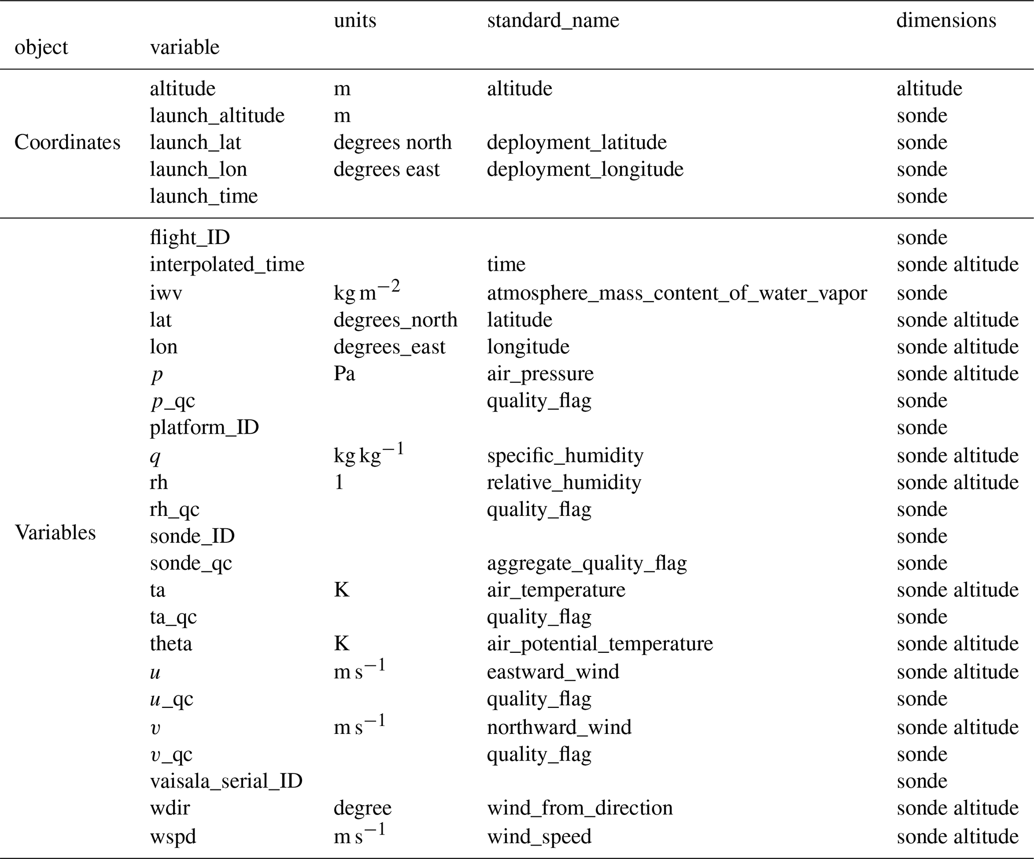
- Appendix C: Variables in Level 3
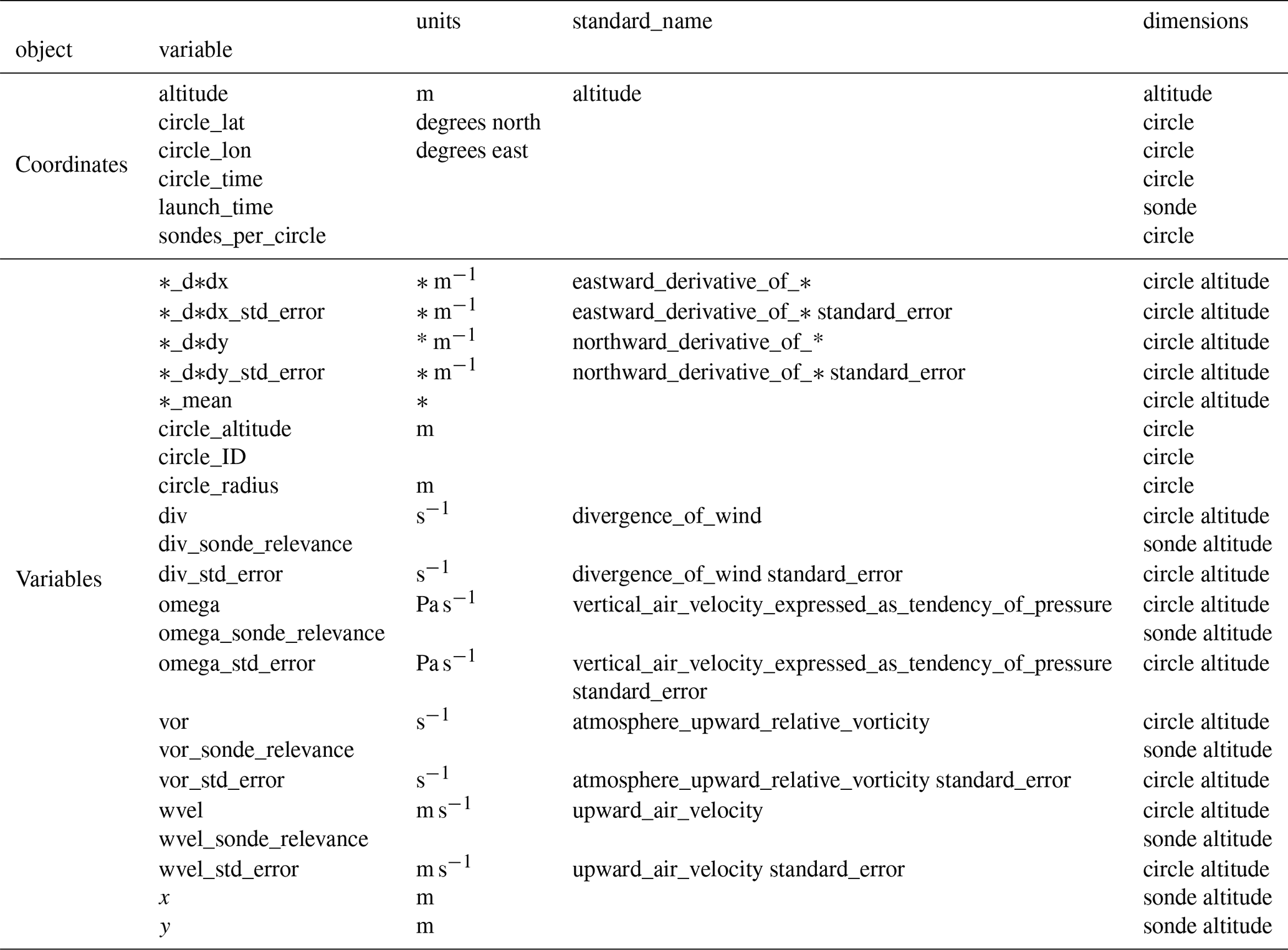
- Appendix D: Variables in Level 4
- Appendix E: Problematic sondes
- Author contributions
- Competing interests
- Disclaimer
- Acknowledgements
- Financial support
- Review statement
- References
- Abstract
- Introduction
- Measurements
- Data Processing and Data Products
- Data overview
- Summary
- Code and data availability
- Appendix A: Glossary
- Appendix B: Setting SAFIRE ATR-42 coordinated measurements into the PERCUSION context
- Appendix C: Variables in Level 3
- Appendix D: Variables in Level 4
- Appendix E: Problematic sondes
- Author contributions
- Competing interests
- Disclaimer
- Acknowledgements
- Financial support
- Review statement
- References