the Creative Commons Attribution 4.0 License.
the Creative Commons Attribution 4.0 License.
 | 26 Jun 2026
Next-generation Metop ASCAT surface soil moisture datasets from EUMETSAT H SAF
Sebastian Hahn
Thomas Melzer
Wolfgang Wagner
This article presents the latest version of the Advanced Scatterometer (ASCAT) surface soil moisture (SSM) dataset provided by the Satellite Application Facility on Support to Operational Hydrology and Water Management (H SAF) lead by the European Organisation for the Exploitation of Meteorological Satellites (EUMETSAT). This new release brings the operational near real-time (NRT) product up to date with the historical offline data record. For years, the H SAF ASCAT SSM data records have benefited from successive algorithmic improvements while the H SAF ASCAT SSM NRT product has only received minor updates until its discontinuation in July 2025. A new processing chain replaces the previous service and applies the latest soil moisture retrieval algorithm to both data streams, creating a unified offline/NRT dataset and representing a major advancement for the H SAF ASCAT SSM NRT product. The H SAF ASCAT SSM climate data record (CDR) covers the time period 1 January 2007 until 31 December 2024, which is extended offline by an interim climate data record (ICDR) as well as in NRT.
The new release also introduces a high-resolution 6.25 km sampling H SAF ASCAT SSM dataset, alongside the standard 12.5 km sampling SSM dataset. This is achieved by customising the spatial resampling process of the ASCAT Level 1B full-resolution backscatter data. A new key development in the algorithm for ASCAT SSM concerns the estimation of the dry and wet backscatter references. Specifically, a moving-window approach is now applied to mitigate artificial trends caused by long-term land cover changes. Furthermore, a new monthly subsurface scattering flag has been added to filter out unreliable SSM measurements where backscatter and soil moisture indicate an inverted relationship.
Quality control of the H SAF ASCAT SSM datasets is performed by using soil moisture estimates from Noah GLDAS-2.1 and the ESA CCI Passive Soil Moisture (SM) v09.1 product, as well as in-situ observations provided by the International Soil Moisture Network (ISMN). The validation results show that both H SAF ASCAT SSM datasets have a comparable performance in terms of the Pearson correlation coefficient (H SAF ASCAT SSM 6.25 km vs ESA CCI Passive SM: 17.9 % > 0.75 and 57.8 % > 0.5; H SAF ASCAT SSM 12.5 km vs ESA CCI Passiv SM: 19.6 % > 0.75 and 59.2 % > 0.5) and signal-to-noise ratio (SNR) derived using triple collocation analysis (H SAF ASCAT SSM 6.25 km SNR: 56.0 % > 0 dB, 35.6 % > 3 dB, H SAF ASCAT SSM 12.5 km SNR: 58.1 % > 0 dB, 38.6 % > 3 dB). The best agreement can be found in regions with strong seasonal variability, including monsoonal, savanna, Mediterranean, and tropical wet-and-dry zones. A weaker consistency can be found in areas characterised by limited soil moisture variability (such as deserts), dense vegetation, pronounced topographic complexity, wetland areas, or higher latitudes (> 60∘ N) experiencing longer periods of frozen soil and snow cover.
The H SAF ASCAT SSM CDR and ICDR datasets (6.25 km sampling: https://doi.org/10.15770/EUM_SAF_H_0012, H SAF, 2025c, and 12.5 km sampling: https://doi.org/10.15770/EUM_SAF_H_0011, H SAF, 2025a) are publicly available online (H SAF, 2025a, c, d, e), while H SAF ASCAT SSM NRT datasets (H SAF, 2025b, f) are distributed via the broadcasting system EUMETCast.
- Article
(6977 KB) - Full-text XML
- BibTeX
- EndNote


Soil moisture information derived from C-band (5.255 GHz) backscatter measurements acquired by the Advanced Scatterometer (ASCAT) has found widespread use in geoscientific applications such as numerical weather prediction, rainfall estimation, flood forecasting and drought monitoring (Dharssi et al., 2011; Draper et al., 2011; Gómez et al., 2020; Aires et al., 2021; Wanders et al., 2014; Brocca et al., 2012, 2014, 2017; Gaona et al., 2025). From the standpoint of the end-user, key advantages of ASCAT surface soil moisture (SSM) data include its operational availability, near-global daily coverage, and the provision of a long-term data record (Wagner et al., 2013). The latter is particularly crucial for studies related to climate change and applications that require consistent historical time series, either for enhancing process understanding or for the calibration of geophysical models. A prominent example is the ESA Climate Change Initiative (CCI) for soil moisture, which incorporates ASCAT SSM data as a core component within its active microwave soil moisture product (Dorigo et al., 2017; Gruber et al., 2019). Furthermore, ASCAT SSM data plays a key role in the operational product suites of both the Copernicus Climate Change Service (C3S) (Copernicus Climate Change Service, 2018) and Copernicus Land Monitoring Service (CLMS) (Bauer-Marschallinger et al., 2018).
In recent years, research on ASCAT soil moisture retrieval has made significant advances focusing on several key areas. These include the dynamic characterisation of the backscatter-incidence angle relationship (Melzer, 2013; Hahn et al., 2017; Vreugdenhil et al., 2017; Steele-Dunne et al., 2019, 2021), spatially-variable vegetation correction (Hahn et al., 2021), and the investigation and modelling of subsurface scattering effects (Morrison and Wagner, 2020; Wagner et al., 2022, 2024). Despite the progress in the dynamic characterisation of the incidence angle dependency of backscatter, a multi-year climatology is still being used in the operational processing chain. This is primarily due to the robustness and near real-time (NRT) suitability. In contrast, the spatially-variable vegetation correction has been successfully integrated and is now used on a regular basis. The study of subsurface scattering effects has provided insights into regions exhibiting an inverse relationship between backscatter and soil moisture. Various statistical and physically-based indicators have been developed to identify these regions, although a global implementation of the newly developed backscatter model remains to be realised. As an interim measure, a monthly subsurface scattering probability flag is now provided as a quality indicator to mask data from affected time periods (Lindorfer et al., 2023).
The aforementioned improvements of the soil moisture retrieval algorithm have been gradually implemented and published as offline ASCAT SSM data record products provided by the Satellite Application Facility on Support to Operational Hydrology and Water Management (H SAF) lead by the European Organisation for the Exploitation of Meteorological Satellites (EUMETSAT) (H SAF, 2018, 2020b, 2021b). However, the ASCAT SSM NRT dataset (EUMETSAT, 2015) produced as part of the EUMETSAT ground segment has never benefited from these algorithmic advancements, due to a separate implementation of the NRT and offline processing chains. The EUMETSAT NRT processing chain has been discontinued on 14 July 2025 and replaced by a new H SAF processing chain, migrating the latest offline soil moisture retrieval improvements to both data streams. This article addresses the newly released H SAF ASCAT SSM datasets, which introduce improvements that mitigate the following limitations previously present in the EUMETSAT NRT processing chain:
-
Model parameter estimation only based on Metop-A ASCAT for the time period 2007–2014
-
Only using a land/water ratio flag during spatial resampling, instead of filtering individual backscatter echos
-
Globally static vegetation correction parameters
-
Long-term land cover changes affecting backscatter trends, propagating into the soil moisture retrieval
-
No information on the effect of subsurface scattering
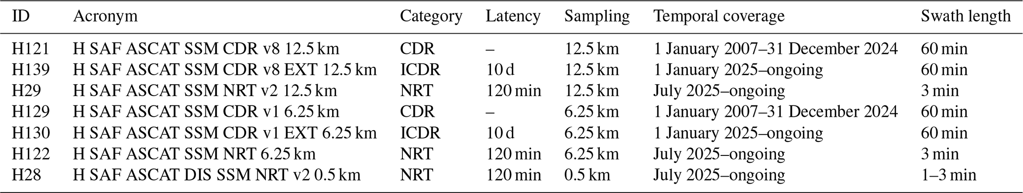
Table 1Coarse resolution soil moisture datasets based on a single microwave instrument – instrument properties and references.
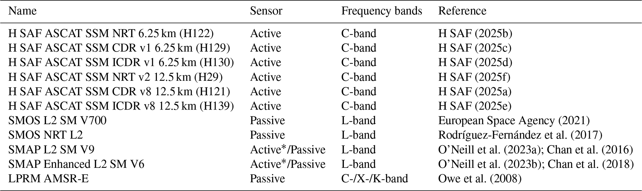
* Instrument failure in July 2015
Table 2Coarse resolution soil moisture datasets based on a single microwave instrument – spatial and temporal properties.
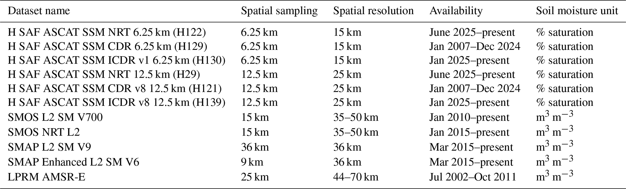
Relative to other (single sensor) remote sensing soil moisture products (see Tables 1 and 2), ASCAT SSM strikes a solid balance between retrieval accuracy and robustness across diverse environmental conditions. While NASA's Soil Moisture Active Passive (SMAP) mission usually performs best overall in validation studies, ESA's Soil Moisture and Ocean Salinity (SMOS) mission and ASCAT SSM are more closely matched, with either holding a slight edge depending on the regional environment or validation methodology (Al-Yaari et al., 2019; Beck et al., 2021; Fan et al., 2022; Kim et al., 2023; Xie et al., 2024). ASCAT SSM excels by providing a stable long-term record, capturing short-term dynamics effectively and its operational availability. Unlike SMAP and SMOS, which offer absolute soil moisture (m3 m−3), ASCAT delivers relative values (% saturation). This allows users to derive absolute soil moisture themselves by combining ASCAT SSM data with their own soil maps. Consequently, it is important to understand that reported metrics such as root mean square difference (RMSD) and bias are linked to the selected conversion approach (e.g. min/max scaling, CDF-matching). Therefore, ASCAT's performance is often evaluated by its dynamic consistency, using scaling-insensitive metrics like temporal correlation and triple collocation analysis (TCA). A more comprehensive assessment of its value, however, comes from indirect applications such as rainfall estimates (SM2Rain) (Brocca et al., 2013, 2019; Kim et al., 2025) or quantifying the improvement in forecast skill achieved through data assimilation (Brocca et al., 2010; Draper et al., 2012; Seo et al., 2021).
In this article we present the latest H SAF ASCAT SSM data release (CDR, ICDR, NRT), which for the first time includes a new high-resolution (6.25 km spatial sampling) dataset alongside the standard 12.5 km spatial sampling version. The theoretical spatial resolution for the new high-resolution dataset is 15 km, defined by the full width at half maximum (FWHM) of the spatial filter. However, the actual effective resolution varies depending on factors such as the number and size of the full-resolution backscatter observations used in the spatial resampling process. Furthermore, both H SAF ASCAT SSM CDR datasets cover the period January 2007 to December 2024 and are continuously extended through both offline processing (ICDR) and near real-time (NRT) updates. Over this time, long-term land cover changes have begun to noticeably affect the underlying backscatter observations, requiring correction to avoid artificial trends in the soil moisture retrievals. For this reason, a new moving-window calibration approach has been introduced to dynamically correct the backscatter signal and prevent non-hydrological long-term trends. In addition, the lower and upper bounds of the backscatter signal are now defined using percentile estimates to improve robustness and better represent local signal variability. As a consequence, the scaling range has been reduced from 0 %–100 % to 5 %–95 % to minimise the likelihood of observations saturating at the dry or wet (percentile) backscatter limits. The performance of both H SAF ASCAT SSM datasets is evaluated using in-situ observations from the International Soil Moisture Network (ISMN), satellite-based reference data from the ESA CCI Passive Soil Moisture product, and model-based soil moisture from NASA's Global Land Data Assimilation System (GLDAS). Hereafter, the H SAF ASCAT SSM datasets are referred to simply as ASCAT SSM datasets.
2.1 ASCAT Level 1B Sigma Zero Full-Resolution (SZF)
The Advanced Scatterometer (ASCAT) is a C-band (5.255 GHz) radar instrument designed to measure the Earth's surface backscatter coefficient, known as the Normalized Radar Cross Section (NRCS) or σ0 expressed in m2 m−2 or dB (Gelsthorpe et al., 2000; Figa-Saldana et al., 2002). At present, ASCAT backscatter measurements are acquired operational onboard the Metop-B and Metop-C satellites. The first satellite in the Metop series (Metop-A) also carried an ASCAT instrument and operated for 15 years before completing its mission in November 2021. The data collected by ASCAT are processed and distributed by the European Organization for the Exploitation of Meteorological Satellites (EUMETSAT) in several product formats.
EUMETSAT provides three types of ASCAT Level 1B backscatter products: Sigma Zero Full-Resolution (SZF), Sigma Zero Research (SZR) and Sigma Zero Operational (SZO). The ASCAT Level 1B SZR and SZO products represent spatially averaged backscatter values provided on orbit grid nodes with a sampling of 12.5 km (SZR) and 25 km (SZO). The ASCAT Level 1B SZF product corresponds to geo-located backscatter values along the six ASCAT beams, which are not collocated and spatially averaged on regular orbit grid nodes. Instead, 192 backscatter observations along every antenna beam projection on the ground are provided. The resolution of each backscatter “echo” varies slightly along the beam, measuring approximately 10 km in the along-beam direction and 25 km in the across-beam direction (Anderson et al., 2012b).
The ASCAT Level 1B SZF backscatter product serves as the primary input for generating the ASCAT surface soil moisture (SSM) datasets. The backscatter measurements are first spatially resampled onto a fixed Earth grid (see Sect. 3.1), after which time series are constructed (see Sect. 3.2). As part of the change detection algorithm, model parameters are empirically estimated and applied to derive the ASCAT SSM datasets at two different spatial resolutions (see Sect. 3.3). ASCAT backscatter observations from all three Metop satellites are used to compute the semi-empirical model parameters (Metop-A: 1 January 2007–15 November 2021, Metop-B: 1 June 2013–31 December 2024, Metop-C: 1 April 2019–31 December 2024) and have been accessed through the EUMETSAT Data Store – https://data.eumetsat.int/ (last access: 1 February 2025).
2.2 ERA5
ERA5 is the fifth generation of the European Centre for Medium-Range Weather Forecasts (ECMWF) reanalysis dataset available from 1940 onward. The reanalysis combines model data with observations from across the world, providing a high-resolution, globally consistent representation of land, ocean, and atmospheric conditions. In this study, we used hourly soil temperature level 1 (stl1) and snow depth (sd) data to identify and exclude periods with frozen soil or snow cover when estimating dry and wet backscatter references (see Sect. 3.3.1). Additionally, these variables were used to compute a climatological frozen soil and snow cover probability flag based on 40 years of data (see Sect. 3.4.3 and 3.4.4). Finally, the same ERA5 variables were also utilized during validation to identify ASCAT SSM observations affected by frozen soil or snow cover (see Sect. 3.5). A spatial and temporal nearest-neighbor matching is used to combine ERA5 with ASCAT SSM data. ERA5 data has been accessed through the Copernicus Climate Data Store – https://cds.climate.copernicus.eu/ (last access: 6 April 2025).
2.3 Noah GLDAS-2.1
The Global Land Data Assimilation System Version 2.1 (GLDAS-2.1) is a state-of-the-art land surface modeling system designed to provide high-resolution global land surface states, including soil moisture, soil temperature, and energy fluxes (Rodell et al., 2004; Beaudoing et al., 2020). One of the primary models used in GLDAS-2.1 is the Noah Land Surface Model (Noah LSM), which provides a physically based representation of soil moisture dynamics by simulating four soil layers at depths of 0–10, 10–40, 40–100, and 100–200 cm. The soil moisture data are provided in kg m−2, three-hourly (00:00, 03:00, 06:00, 09:00, 12:00, 15:00, 18:00, and 21:00 UTC) and monthly averages at a spatial sampling of 0.25° (∼ 25 km), making it suitable for global and regional hydrological assessments. In this study, we used soil moisture information from the first layer (0–10 cm) of the three-hourly GLDAS-2.1 product as an independent reference dataset for validating the ASCAT SSM datasets (see Sect. 3.5). A spatial and temporal nearest-neighbor matching is used to combine GLDAS-2.1 with ASCAT SSM data. GLDAS-2.1 data has been accessed through the Goddard Earth Sciences Data and Information Services Center (GES DISC) – https://disc.gsfc.nasa.gov/ (last access: 6 April 2025).
2.4 ESA CCI Passive Soil Moisture
The ESA CCI Passive Soil Moisture (SM) v09.1 product is a global dataset developed by the European Space Agency's Climate Change Initiative (ESA CCI), designed to provide consistent long-term soil moisture information based on passive microwave remote sensing observations from Nimbus 7 SMMR, DMSP SSM/I, TRMM TMI, Aqua AMSR-E, Coriolis WindSat, GCOM-W1 AMSR2, SMOS and SMAP (Dorigo et al., 2017; Gruber et al., 2019). The ESA CCI Passive SM v09.1 product covers the period from 1978 to 2023, with a spatial sampling of 0.25° (∼ 25 km) and a daily temporal resolution, expressed in volumetric soil moisture units (m3 m−3). The ESA CCI Passive SM v09.1 product is used as an independent reference for validating the ASCAT SSM datasets (see Sect. 3.5). A spatial and temporal nearest-neighbor matching is used to combine CCI SM with ASCAT SSM data. ESA CCI SM data has been accessed through the Centre for Environmental Data Analysis Archive – Earth Observation Data – https://catalogue.ceda.ac.uk/ (last access: 14 July 2025).
2.5 ESA CCI Land Cover
The ESA CCI Land Cover (LC) dataset provides global land cover maps from 1992 to 2022 at a spatial resolution of 300 m (ESA, 2017). Version 2.0.7 covers the period 1992–2015, while version 2.1.1 extends the record from 2016 onwards. Both versions are produced using the same processing chain to ensure temporal consistency across the entire dataset. Each annual map is generated by detecting land cover changes relative to a unique baseline LC map, which is derived from the Medium Resolution Imaging Spectrometer (MERIS) Full Resolution (FR) and Reduced Resolution (RR) archive covering 2003–2012. ESA CCI LC data has been accessed through the Centre for Environmental Data Analysis Archive – Earth Observation Data – https://catalogue.ceda.ac.uk/ (last access: 5 December 2024).
The ESA CCI LC map for 2018 is used to compute a fractional LC dataset, spatially aligned with the resolution of ASCAT backscatter measurements. This dataset is used to identify and exclude unwanted backscatter signals originating from lakes, urban areas, and open water (see Sect. 3.1).
2.6 Global Lakes and Wetlands Database (GLWD)
The Global Lakes and Wetlands Database (GLWD) v1 represents a combination of existing data sources for lakes and wetlands on a global scale (Lehner and Döll, 2004). The database focuses on three level: (i) large lakes and reservoirs, (ii) smaller water bodies and (iii) wetlands. In this study, the GLWD dataset is used to calculate the wetland fraction flag (see Sect. 3.4.1). A spatial nearest-neighbor matching is used to combine GLWD with ASCAT SSM data. The GLWD v1 data were originally published by the World Wildlife Fund (WWF) but are no longer available on their website. However, the dataset can be accessed through Data Basin at https://databasin.org/ (last access: 3 March 2015).
2.7 Copernicus DEM
The Copernicus Digital Elevation Model (Copernicus DEM) is a global Digital Surface Model (DSM) that represents the elevation of the Earth's surface, including natural terrain features and built structures (Copernicus, 2021). It is derived from data acquired by the TanDEM-X satellite mission between 2011 and 2015. In this study, the 90 m spatial resolution version of the Copernicus DEM (GLO-90) is used for the calculation of the topographic complexity flag spatially matched to the ASCAT data (see Sect. 3.4.2). The Copernicus DEM has been accessed through the Copernicus Dataspace – https://dataspace.copernicus.eu/ (last access: 6 February 2025).
2.8 Global Subsurface Scattering Maps
Wagner et al. (2024) developed global maps that identify areas influenced by subsurface scattering, using both statistical analyses and physically-based indicators (Lindorfer et al., 2023). Subsurface scattering can induce an inverse relationship between backscatter and soil moisture, thereby compromising the interpretation of backscatter variations in the ASCAT soil moisture change detection algorithm. Although a recently developed backscatter model, which includes a subsurface scattering term, successfully explained backscatter anomalies in arid environments (Wagner et al., 2022), its implementation at the global scale is still pending. Consequently, the ASCAT SSM datasets must be masked for spatial and temporal subsurface scattering effects. A monthly probability of backscatter anomalies from Wagner et al. (2024) is provided as part of the ASCAT SSM datasets and applied during validation (see Sect. 3.5). Subsurface scattering maps have been access through the TU Wien research data portal – https://researchdata.tuwien.ac.at/ (last access: 7 April 2025).
2.9 In-situ data
The International Soil Moisture Network (ISMN) serves as a data portal that maintains global in-situ soil moisture observations (Dorigo et al., 2011, 2021). A collaborative effort among various network operators helps to collect and maintain in-situ data worldwide. The primary objective of the ISMN soil moisture database is to provide ground reference data for the validation of satellite soil moisture products. In this study, we selected a total number of 43 in-situ networks containing sensors with a depth range of 0–10 cm. The list of ISMN networks can be found in Table B1. The spatial and temporal extent of these networks is variable, as well as their land cover and climate characteristics. Smaller networks with less stations represent very local conditions (e.g. DAHRA,, IIT_KANPUR, LAB-net, LABLUX, SKKU, VAS), while larger networks cover a number of different climate zones and land cover classes (e.g. SCAN, SNOTEL, USCRN). A spatial and temporal nearest-neighbor matching is used to combine ISMN with ASCAT data. The ISMN data has been accessed through the ISMN data portal – https://ismn.earth/ (last access: 31 March 2026).
The ASCAT Surface Soil Moisture (SSM) datasets are based on a physically-based change detection approach, which was initially developed for backscatter observations from ERS-1/-2 (Wagner et al., 1999a, b, c; Scipal et al., 2002). This method takes advantage of the strong dependency of the radar backscatter intensity to variations in soil moisture content. As soil moisture increases, the dielectric constant at the air-soil interface also rises, resulting in a stronger backscatter signal (Wagner et al., 2013). However, recent research has also shown that under special circumstances subsurface scattering can induce an inverse relationship, most notably in arid environments with strong scatterers beneath shallow soil (Wagner et al., 2022, 2024). Therefore, an accurate quantification and mitigation of such subsurface scattering effects has become a major focus of research.
The change detection algorithm relies on calibrated model parameters, which are independently estimated for each location using historical backscatter observations. Therefore, as part of the pre-processing procedure, a time series of backscatter observations is generated from spatially resampled ASCAT Level 1B Sigma0 Zero Full-Resolution (SZF) swath data. The semi-empirical model parameters are needed to model and correct azimuth and incidence angle effects and to scale normalised backscatter observations between dry and wet backscatter references. The resulting soil moisture estimates are expressed in degree of saturation, ranging from 0 % (dry) to 100 % (saturated soil) representing the topsoil layer (< 5 cm).
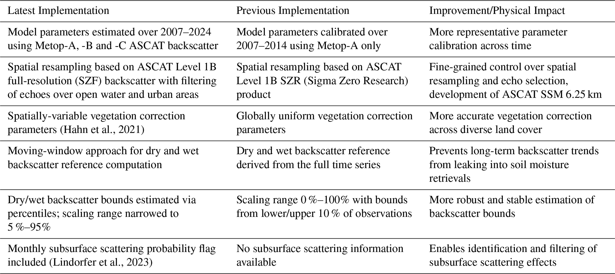
It is important to note that the creation of the backscatter time series and the estimation of semi-empirical model parameters are carried out offline. By computing all necessary parameters in advance, the soil moisture retrieval can be efficiently performed on the original ASCAT Level 1B Sigma0 Zero Full-Resolution (SZF) swath data. This setup also allows a near real-time (NRT) application of the change detection method. Figure 1 provides an overview of the entire workflow, with each step described in more detail in the following subsections and Table 3 presents a summary of the key algorithmic advancements compared to the previous ASCAT SSM NRT product.
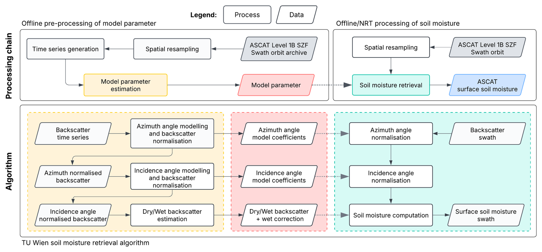
Figure 1Overview of the processing workflows and retrieval algorithm. The upper flowchart illustrates the offline model parameter pre-processing steps and the offline/NRT surface soil moisture processing chain. The lower flowchart provides a detailed summary of the TU Wien soil moisture retrieval algorithm.
Table 3Comparison of latest and previous ASCAT SSM retrieval implementations.
Updating the soil moisture retrieval model parameters modifies both the climatological mean and the temporal dynamics of the ASCAT SSM datasets, resulting in inconsistencies with the previous ASCAT SSM NRT version. Consequently, data assimilation systems cannot transition to the new ASCAT SSM dataset without prior recalibration.
3.1 Spatial resampling
3.1.1 Aggregation and filtering
The ASCAT Level 1B Sigma Zero Full-resolution (SZF) dataset contains backscatter observations σ0 (also called “echos”) at very high spatial resolution for each antenna beam (Fore, Mid, Aft), which are spatially not perfectly collocated. The spatial extent, shape, and orientation of an individual echo is determined by the observation geometry, on-board processing in range and Doppler frequency. The spatial response function (SRF) is used to describe how the backscatter signal is weighted across the surface footprint (Lindsley et al., 2016; Vogelzang et al., 2017).
The spatial resampling process aims to generate consistent backscatter triplets at a coarser spatial resolution by filtering and aggregating echos from individual beams, thereby also reducing inherent observational noise. The spatial extent and resolution is given by its cumulative spatial response function (CSRF) determined by the window function and its associated spatial radius applied during the aggregation of the echos. Backscatter is first converted from the decibel scale to the linear domain, where a weighted average is computed. The averaged backscatter is then converted back to the decibel scale. A weighted average is also applied to the incidence and azimuth angles, providing a consistent representation of the observation geometry. In addition, the normalized noise variance (known as kp-value) is also derived for the averaged backscatter, representing the relative standard deviation of the noise within the averaging area (see Eq. 1). The kp-value not only reflects natural surface heterogeneity but also noise contributions (Anderson et al., 2012a).
A Hamming window (see Eq. 2) with a spatial radius (X) of approximately 14 km is applied to generate backscatter triplets sampled at a grid spacing of 6.25 km, yielding a theoretical spatial resolution of 15 km. This theoretical resolution is defined by the full width at half maximum (FWHM) of the spatial filter (Figa-Saldana et al., 2002). The actual spatial resolution, however, cannot be determined precisely since it varies depending on factors such as the number and size of the full-resolution backscatter observations used in the spatial resampling process. However, the effective spatial resolution closely approximates the theoretical resolution due to the application and size of the Hamming window. Unlike the ASCAT Level 1B SZR and SZO datasets provided by EUMETSAT, which are sampled on orbit-specific grid nodes, the backscatter triplets are located on a fixed Earth grid. This approach allows the resampled ASCAT Level 1B SZF backscatter data to be easily stacked, enabling the construction of a time series during subsequent processing. The weights (w) for a backscatter echo with a distance x are computed using the following equation:
Additionally, a second backscatter triplet dataset is also generated at a coarser grid spacing of 12.5 km, using a spatial radius of 24 km, resulting in a theoretical spatial resolution of 25 km. Both backscatter triplet datasets are independently used to produce two ASCAT surface soil moisture (SSM) datasets, sampled at 6.25 and 12.5 km, respectively. The 12.5 km sampling corresponds to the standard spatial sampling distance also used by the ASCAT Level 1B SZR product, whereas the 6.25 km dataset is designed to maximise spatial detail while retaining an acceptable noise level.
Not all backscatter echos are included in the aggregation process. Echos located over areas not sensitive to soil moisture changes (open water, coastal regions, urban areas) are excluded. The identification of these echos is achieved using the ESA CCI Land Cover dataset (v2.1.1), which is pre-processed to represent a fractional land cover dataset, aligned with the spatial resolution of the backscatter echos. This way, unwanted backscatter observations are determined and filtered. In addition, an outlier detection method based on the Median Absolute Deviation (MAD) is applied per beam for all echos () to further refine the spatially resampled dataset by removing echos that deviate significantly from the expected behaviour (), ensuring the reliability of the aggregated backscatter data.
It should be emphasised that the ASCAT Level 1B SZF dataset is spatially resampled into 60 min segments to avoid any ambiguity caused by a spatial overlap. To ensure complete sampling of the swath edges, a temporal buffer is added at both the beginning and end of each segment (±5 min), allowing all relevant echos to be included. In a near real-time processing scenario, the segments are much smaller (≈ 3 min), but a temporal buffer is still needed to include all relevant backscatter observations.
3.1.2 Fibonacci grid
The Fibonacci grid was selected as the fixed Earth reference grid. It is designed to uniformly distribute points across the surface of a sphere. Inspired by the Fibonacci sequence and the golden ratio (), it ensures a nearly equal-area distribution of points. Constructing the grid involves distributing points along the vertical axis of the sphere (latitude) and rotating them around the sphere's horizontal axis (longitude) based on the complementary golden angle (360). This deterministic approach is computationally efficient and scales easily by adjusting the number of points. Unlike traditional latitude-longitude grids (e.g. 1°× 1°), the Fibonacci grid systematically spaces points to avoid clustering at the poles. The Fibonacci grid points, initially calculated on a sphere, are transformed into ellipsoidal coordinates to align with the coordinate reference system used to geo-locate ASCAT backscatter data (WGS84). However, this transformation alters distances between points on a larger scale due to differences in curvature between the sphere and the ellipsoid. Fortunately, only short distances (< 25 km) are relevant for the resampling process, minimising the impact of the coordinate transformation.
The Fibonacci grid is generated using the following formulas (González, 2009). The absolute number of points P is defined by a natural number N, which is the only parameter to be determined to generate a Fibonacci grid.
The spherical coordinates (expressed in radians) of the ith point are
The Fibonacci grid representing an approximate sampling of 6.25 km is composed of 13 200 001 points (N=6 600 000), whereas the approximate sampling of 12.5 km is realised by 3 300 001 points (N=1 650 000). In both cases, only one-third of the grid points are situated over land surfaces. An example of the 12.5 km Fibonacci grid is shown in Fig. 2.
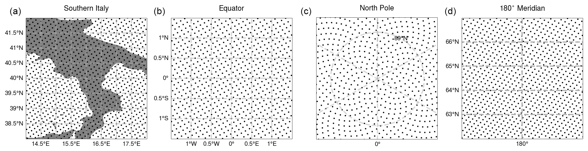
Figure 2Fibonacci grid with 12.5 km sampling is shown for (a) Southern Italy, (b) the Equator, (c) the North Pole, and (d) the 180° meridian.
In the context of the ASCAT SSM dataset, the Fibonacci grid is used as a discrete global grid (DGG) that offers uniform sampling of the Earth's surface. Data stored on this grid consist a collection of geolocated points (EPSG:4326), requiring no specialized software for processing or interpretation.
3.2 Backscatter time series
The resampled backscatter swath segments are stored according to the Climate and Forecast (CF) point data model (Eaton et al., 2024), which standardises the representation of individual geo-referenced observations. In the next step, the point data are systematically transformed into the CF index ragged array format, a data structure tailored for time series representation. In this new format, all point observations are consolidated into a single array, while an index variable links each observation to its corresponding location on the fixed Earth grid. This approach facilitates a flexible and scalable storage of time series data for each grid location. Furthermore, the data format supports integrating any future observations, allowing a seamless extension of the time series. Optionally, the final time series can be converted into the CF contiguous ragged array format, which optimises data access performance by ensuring a chronological sorting for each grid location. However, this format compromises the ease of future data extension due its strict sorting structure. More specifically, a contiguous ragged array stores chronologically ordered data for multiple grid points as a single contiguous block. While this data structure allows efficient data access, inserting data out-of-order (e.g., from earlier grid points) will corrupt both. Avoiding this problem requires inserting data at its correct chronological position which, would require a large amount of I/O operations (i.e. shifting elements, rewriting datasets).
3.3 TU Wien change detection algorithm and model parameter estimation
The semi-empirical change detection method has been developed by the Vienna University of Technology (TU Wien) and was initially applied to backscatter observations acquired by the Advanced Microwave Instrument (AMI) on-board the ERS-1 and ERS-2 satellites (Wagner et al., 1999a, b, c; Scipal et al., 2002). Thanks to a similar instrument design, the same methodology was later successfully adapted for the Advanced Scatterometer (ASCAT) on-board the series of Metop satellites (Bartalis et al., 2006b, 2007; Naeimi et al., 2009a, b). The change detection method eliminates the need for explicit surface roughness parameterisation and leverages multi-incidence angle backscatter observations to simultaneously model soil moisture and vegetation dynamics (Wagner et al., 2013). From a mathematical perspective, the change detection method is simpler than a radiative transfer model and can be solved directly without the need for a non-linear iterative optimisation.
The backscatter triplet dataset in time series format serves as input for the model parameter estimation procedure. Backscatter varies primarily due to surface dielectric properties, roughness, and vegetation, which are the most influential factors. Additionally, its overall magnitude is strongly affected by the measurement geometry, i.e. the incidence angle (θ) and the azimuth angle (ϕ). To accurately attribute backscatter variations to changes in soil moisture, both the azimuth and incidence angle dependencies of backscatter must be addressed. Section A summarizes these steps for the TU Wien change detection algorithm, along with the computation of the estimated backscatter standard deviation and the underlying error propagation. The following discussion of the TU Wien change detection algorithm focuses only on the latest major updates.
3.3.1 Estimation of dry and wet backscatter reference
The dry and wet backscatter references represent the lower and upper bounds of backscatter associated with dry and wet soil conditions, respectively. These references are essential because they compensate for static (e.g. surface roughness) and dynamic influences (e.g. vegetation phenology) on the backscatter signal. By scaling backscatter observations to these bounds, signal variations should primarily reflect relative changes in soil moisture, minimising the impact of other effects. Furthermore, observations taken during periods of frozen soil and snow cover are excluded from the computation. Although frozen soil and dry soil have similarly low dielectric constants, in practice, backscatter values can decrease substantially under frozen conditions, making them unsuitable for defining the dry reference.
Traditionally, the dry and wet backscatter references have been estimated from the entire backscatter time series, which has proven effective over periods of 3 to 8 years. However, as the record now spans more than 15 years, long-term land cover changes have become a significant source of trends in backscatter, such as deforestation or urbanisation. Therefore, a monthly estimation approach using a moving window of ±42 months (i.e. ±3.5 years) has been implemented. This way, the dry and wet backscatter reference are able to gradually adapt to non-soil moisture related changes over time.
The dry and wet soil conditions are derived by interpolating all backscatter observations to specific incidence angles, where their (effective) minimum/maximum is computed (see Eqs. 7 and 8). These angles, known as the dry and wet cross-over angles (θd, θw), are selected to minimise the influence of vegetation. The initial values were empirically set to θd=25° and θw=40° and applied globally (Wagner et al., 1999b, c, a). More recently, these parameters have been spatially parameterised to better account for seasonal vegetation effects (Hahn et al., 2021), and this updated approach has been applied.
with and .
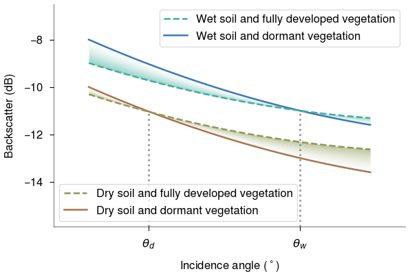
Figure 3A visualization of the cross-over concept: Backscatter-incidence angle curves for constant soil moisture and varying vegetation intersect at characteristic angles where the influence of vegetation on backscatter is minimized. These angles, called the dry and wet cross-over angles, are chosen to minimize the effect of vegetation during the estimation of the dry and wet backscatter reference.
The selection of these specific angles is motivated by the so-called cross-over angle concept (Wagner et al., 1999a), according to which the backscatter-incidence angle curves for constant soil moisture and different vegetation states intersect at a characteristic angle where the effect of vegetation on the backscatter is minimised. By using these cross-over angles, it is possible to isolate soil moisture signals from vegetation influences and obtain reliable dry and wet references. At these angles, the lower (dry) and upper (wet) bounds of the backscatter distribution are derived using the 2nd and 98th percentiles (P2, P98) computed within a ± 42-month moving window centred on each calendar month (see Eqs. 9 and 10), e.g. the target month of August 2015 would include the time period from February 2012 to February 2019. These values are subsequently converted back to the reference incidence angle, which also changes the temporal resolution from monthly to daily due to slope and curvature parameters (see Eqs. 11 and 12).
with mj being the month of interest, month (ti) the month of the observation time stamp, measurements within the current time window and the dry reference at the dry cross-over angle. Similarly, the wet reference, , is computed as the 98th percentile. The selection of these specific percentiles was empirically determined to provide stable and representative reference bounds.
In arid and semi-arid regions, soils rarely become saturated, so a wet correction is applied (see Sect. A4.2). It should be noted that the dry and wet backscatter references, as well as the slope and curvature parameters, are provided with daily time stamps (d) and are converted to backscatter observation time stamps when required. If multiple backscatter observations occur on the same day, the corresponding reference values are assigned identically to each observation.
3.3.2 Soil moisture computation
Backscatter observations are scaled between the dry and wet references to yield relative soil moisture, expressed as degree of saturation from 0 % (dry soil) to 100 % (saturated soil). Notably, the dry and wet backscatter reference values reflect extreme conditions based on historical observations, and are derived using percentile estimation. To account for the associated uncertainty and variability, backscatter observations are scaled between 5 % and 95 % saturation (i.e., a=5 %, b=95 %), as defined in Eq. (13). This approach also aims to minimise the risk of mapping sequences of either low or high backscatter values to extreme soil moisture levels, as this can negatively impact e.g. drought indicators. Furthermore, mild outliers identified by soil moisture values in the intervals −20 %–0 % and 100 %–120 %, are set to 0 % and 100 %, respectively. Strong outliers, defined as less than −20 % or more than 120 % are assigned a value of NaN.
3.4 Advisory flags
Along with the ASCAT SSM datasets, advisory flags are provided to give context on soil conditions, land cover, and scattering behaviour. As previously mentioned, the error model does not account for all potential error sources. These flags complement the error model by helping to identify and filter spatial and temporal situations where soil moisture retrieval may be unreliable.
3.4.1 Wetland fraction flag
As the C-band pulses do not penetrate into water, backscatter characteristics are primarily controlled by the roughness of the water. A calm water surface behaves as a specular reflector, directing almost the entire signal away from the sensor. In contrast, wind-induced waves increase backscatter in both upwind and downwind directions while reducing the signal observed perpendicular to the wind. Consequently, extensive open water within the sensor footprint can significantly interfere with the retrieval of soil moisture. Areas with (temporary) standing water therefore require careful consideration. To address this, information on the extent of lakes, reservoirs, and large rivers is incorporated by aggregating pixel counts within a defined spatial window, thereby quantifying the maximum water body coverage for each area on a scale from 0 % to 100 %.
The wetland fraction flag only indicates the presence of surface water and does not quantify the specific degree of influence a water body may have on the backscatter signal, as this effect can vary depending on factors such as water body size, orientation, or local wind conditions.
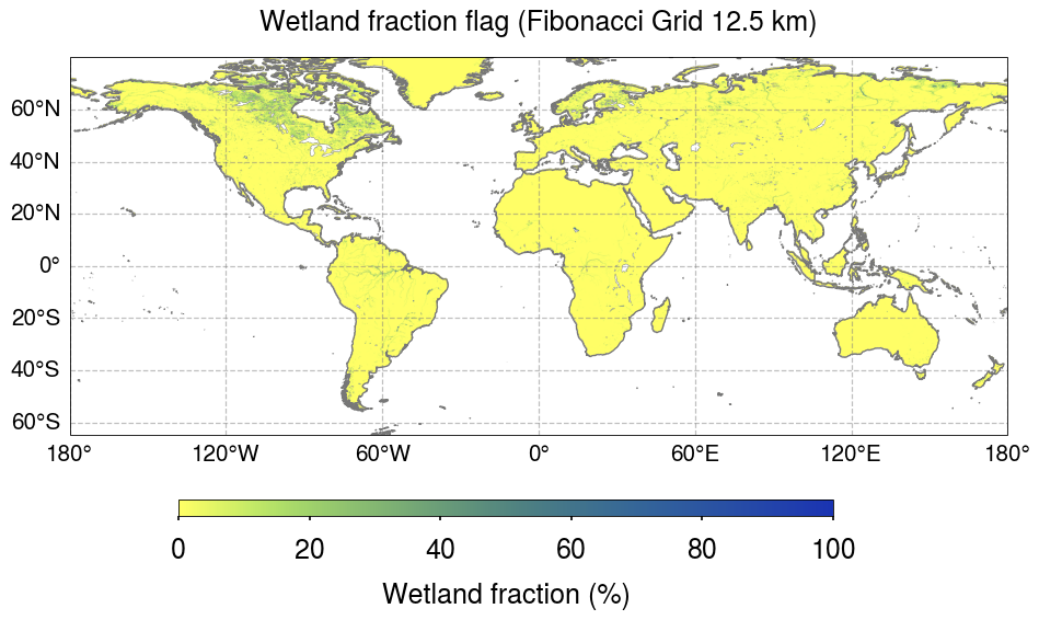
Figure 4Wetland fraction flag on the Fibonacci Grid 12.5 km.
3.4.2 Topographic complexity flag
Land surfaces characterized by rough terrain and mountainous regions are particularly vulnerable to distortions in backscatter signals arising from varying viewing geometries. Such variability in backscatter adversely affects the accurate retrieval of soil moisture dynamics. To address this limitation, a topographic complexity flag has been introduced. This flag is derived from the Copernicus Digital Elevation Model (COP-DEM) at a spatial resolution of 90 m and provides a quantitative measure of topographic variability. Specifically, it is calculated as the standard deviation of elevation and normalised to a scale from 0 % to 100 %. While observation noise is typically higher in topographically complex regions, the topographic complexity flag offers users an additional criterion to identify and mask such areas.
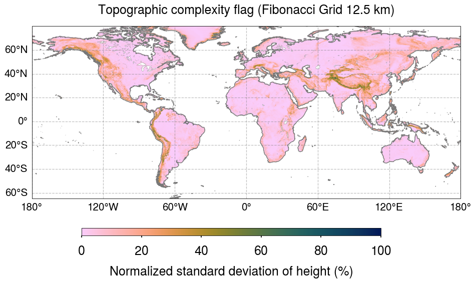
Figure 5Topographic complexity flag on the Fibonacci Grid 12.5 km.
3.4.3 Frozen soil probability
When the soil is frozen, microwave backscatter drops significantly due to restricted mobility of soil water molecules, which limits their dielectric response (Hallikainen et al., 1985; Ulaby et al., 1982). In vegetated areas, the interpretation of the backscatter signal becomes more complex because the water content and physical structure of the vegetation further influence the microwave response. Handling backscatter from soil freezing periods is not covered by the soil moisture retrieval algorithm and affected time periods need to be masked based on auxiliary information.
To quantify the likelihood of soil freezing, we derived the frozen soil probability from ERA5 soil temperature (1980–2020). For each grid point and day of year, the probability is defined as the fraction of years with soil temperatures below 0 °C.
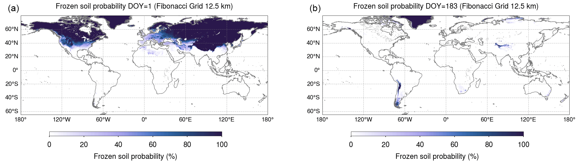
Figure 6Frozen soil probability flag for (a) day of year (DOY) 1, corresponding to 1 January, and (b) DOY 183, corresponding to 1 July on the Fibonacci Grid 12.5 km.
3.4.4 Snow cover probability
The interaction of microwave backscatter with snow is governed by various physical properties of the snow layer, including liquid water content, roughness of the air-snow interface, depth and layering of the snow pack, grain size and shape (Hallikainen et al., 1986; Ulaby et al., 1986). These properties influence the overall backscatter signal through distinct scattering mechanisms (Wismann, 2000). Snow-related scattering effects are not treated in the soil moisture retrieval algorithm and snow covered periods need to be masked based on auxiliary information, e.g. using snow cover information from a land surface model.
Similar to the frozen soil probability, we computed a daily snow probability using ERA5 snow depth data over a 40-year period (1980–2020). For each grid point and day of year, the snow probability is defined as the fraction of years in which snow depth exceeded zero.
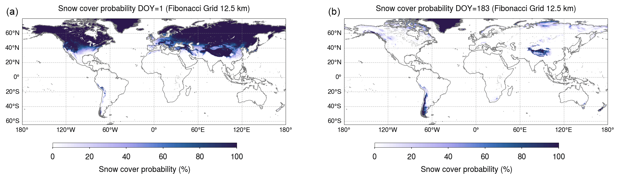
Figure 7Snow cover probability flag for (a) day of year (DOY) 1, corresponding to 1 January, and (b) DOY 183, corresponding to 1 July on the Fibonacci Grid 12.5 km.
3.5 Validation procedure
Quality control of the ASCAT SSM datasets follows standardised validation methodologies for satellite-based Earth observation products (Loew et al., 2017; Land Product Validation Subgroup, 2020). This process involves quality checking and harmonisation of the reference and ancillary datasets, followed by their spatial and temporal collocation to allow consistent inter-comparison. Finally, relevant quality metrics are calculated and systematically analysed.
For the ASCAT SSM datasets, quality control is performed using soil moisture estimates from Noah GLDAS-2.1 and the ESA CCI Passive Soil Moisture (SM) v09.1 product, as well as in-situ observations provided by the International Soil Moisture Network (ISMN). Ancillary information provided by ERA5 is used to filter out ASCAT SSM observations influenced by frozen soil (skin temperature < 0 °C) or snow cover (> 0 m). Additionally, internal quality flags from the ASCAT SSM datasets are applied to mask observations affected by subsurface scattering (subsurface scattering probability > 5 %).
In case of the global analysis against ESA CCI Passive SM and GLDAS-2.1, the fixed Earth grid of the ASCAT SSM datasets served as the spatial reference, with all other datasets collocated using a nearest neighbour search. Temporal collocation is based on the measurement times of the ASCAT SSM datasets. For each ASCAT SSM observation, the temporally closest reference measurement within an 12 h window is selected. The Pearson correlation coefficient (R) and Signal-to-Noise Ratio (SNR) are used as the two main quality metrics. While Pearson R quantifies the strength and direction of a linear relationship between two datasets, SNR is derived from triple collocation analysis (TCA) (Stoffelen, 1998), which estimates error variance by comparing three independent datasets. By relating the error variance to the signal variance, the SNR quantifies the relative strength between the signal and noise. Expressed in decibel (dB), the SNR provides an intuitive interpretation (Gruber et al., 2016). Notably, Pearson R and SNR are both scale-invariant metrics that depend only on the temporal variability structure of the datasets rather than their absolute units. Thus, both metrics can be computed without rescaling ASCAT SSM data from % saturation into m3 m−3.
The Quality Assurance Service for Satellite Soil Moisture Data (QA4SM) was used for the validation against ISMN observations (AWST et al., 2025). ASCAT SSM time series were extracted from the grid points nearest to the ISMN station coordinates and uploaded to the QA4SM portal. ISMN networks with sensors overlapping in time with the ASCAT SSM datasets and operating within the 0–10 cm depth range were selected. A 12 h matching window was applied to identify the nearest observation in time and Pearson R served as the primary performance metric.
4.1 H SAF ASCAT Surface Soil Moisture datasets
As described in Sect. 3, the ASCAT SSM datasets are generated with two spatial sampling distances: 6.25 and 12.5 km. These datasets are distributed as part of the EUMETSAT Satellite Application Facility on Support to Operational Hydrology and Water Management (H SAF) product suite. H SAF aims to provide remote sensing products of hydrological parameters including instantaneous rain rate and accumulated rainfall, surface soil moisture and root zone soil moisture, as well as snow cover and snow water equivalent.
H SAF products are categorized based on their timeliness into three categories: near real-time (NRT), offline, and data records (DR). NRT products offer the lowest latency, providing rapid access. Offline products are available on a daily, weekly, or monthly basis, accommodating a range of applications. DR products represent fixed datasets with well defined start and end dates, suitable for climate analysis. If a DR product spans more than 15 years, it qualifies as a climate data record (CDR). Furthermore, if an offline product uses the same processing chain and input data as a (C)DR and serves to extend it beyond its original time span, it is referred to as an interim data record (IDR) or interim climate data record (ICDR).
The ASCAT SSM datasets are provided as NRT, CDR, and ICDR products as outlined in Table 4. All datasets are available through the H SAF online archive, while NRT products are additionally distributed via EUMETCast, a satellite-based broadcast system operated by EUMETSAT. The primary data format is netCDF, with BUFR (Binary Universal Form for the Representation of meteorological data) being also available for selected products.
Table 4H SAF ASCAT Soil Surface Moisture (SSM) datasets are classified as Level 2 products, except for the Disaggregated (DIS) ASCAT SSM NRT v2 0.5 km product, which is Level 3 product since it represents a downscaled version of the ASCAT SSM NRT 6.25 km product. All products are available in NetCDF file format. ASCAT SSM NRT products (H121, H29) are also available in BUFR file format.
4.1.1 Data characteristics
The ASCAT SSM datasets are supplied in swath orbit geometry, with observations resampled onto a fixed Earth grid. For this purpose, the Fibonacci grid has been selected (see Sect. 3.1.2), ensuring a homogeneous sampling of the Earth's surface. The ASCAT SSM CDR and ICDR consists of swath data covering 60 min interval, whereas the ASCAT SSM NRT datasets are distributed in 3 min product dissemination units (PDUs). Figure 8 shows an example for both swath intervals. All ASCAT SSM datasets (CDR, ICDR, NRT) delivered in netCDF contain an identical set of variables, as listed in Table 5. However, only the ASCAT SSM NRT datasets contain NRT information about soil freezing and snow cover derived from ECMWF forecast data stored in the surface flag variable.
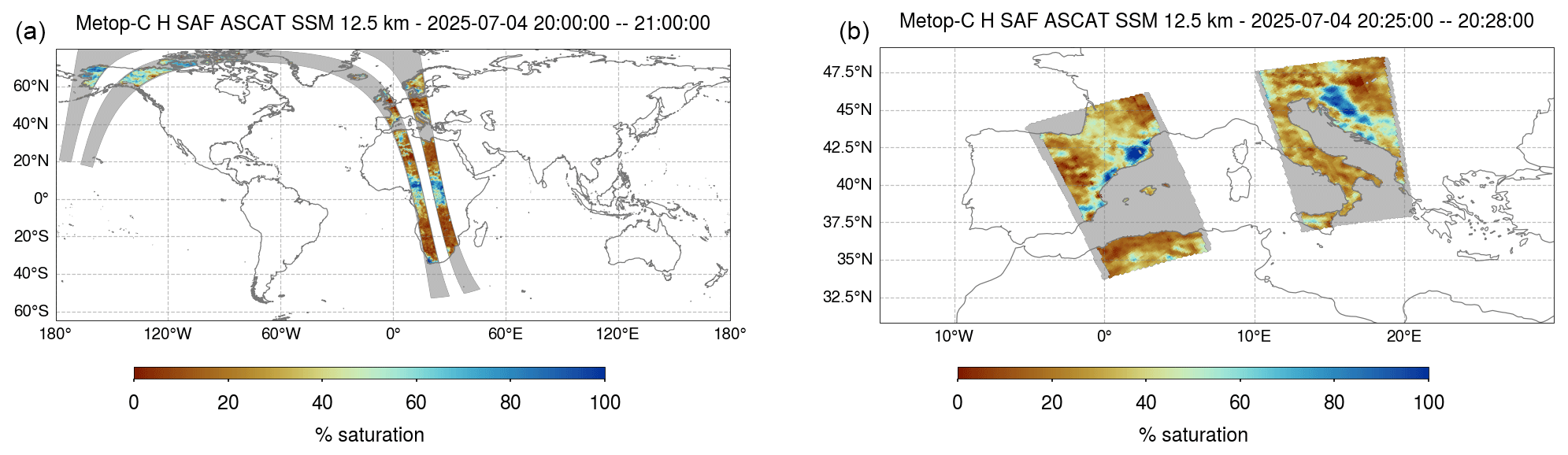
Figure 8Example H SAF ASCAT SSM swath for a 60 min (a) and 3 min (b) interval. ASCAT SSM data © EUMETSAT.
Table 5Description of H SAF ASCAT SSM dataset variables and associated metadata.
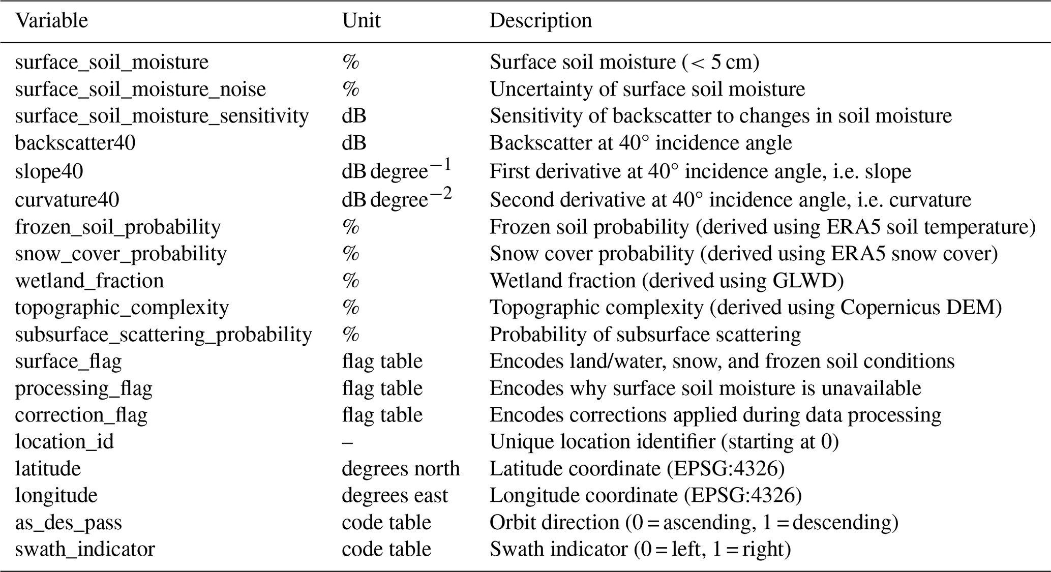
Surface soil moisture (SSM) and its associated noise are the primary variables provided in the ASCAT SSM datasets. Both, SSM and SSM noise are expressed in degree of saturation representing the topmost soil layer (< 5 cm). The SSM sensitivity is quantified in decibels (dB) and defined as the difference between the wet and dry backscatter references for a given day (see Sect. A4.2). It also serves as an indicator of retrieval uncertainty with values below 1 dB typically pointing to densely vegetated areas with a low backscatter signal variation. Backscatter at 40° incidence angle, as well as the first and second derivatives (slope and curvature) of the incidence angle dependency of backscatter, are included to provide additional information. Furthermore, flags inform about surface conditions or processing details (see Sect. 3.4). Time and geo-location parameters are expressed as fractions of days since the reference date 1 January 1970 00:00:00 UTC and latitude/longitude coordinates (EPSG:4326) along with a unique location identifier. Moreover, satellite orbit direction (ascending/descending) and swath identification (left/right) are included.
Since ASCAT SSM datasets are provided on a fixed Earth grid, time series can be readily generated by stacking individual swath segments. As each observation is associated with a unique timestamp and the number of observations varies by location, not all locations have the same number of measurements. Therefore, storing the time series data as an indexed ragged array is more storage-efficient than using an incomplete multidimensional array representation, which requires padding unused elements with missing values. If all locations share the same number of observations, the latter is referred to as an orthogonal multidimensional array representation. Space-time cubes derived from gridded raster data are a classical example. However, it is not well suited for observations from polar-orbiting LEO satellites, where coverage varies due to the swath geometry and orbital dynamics. Figure 9 illustrates the spatial coverage of ASCAT for a single and two Metop satellites over a 24 h period.
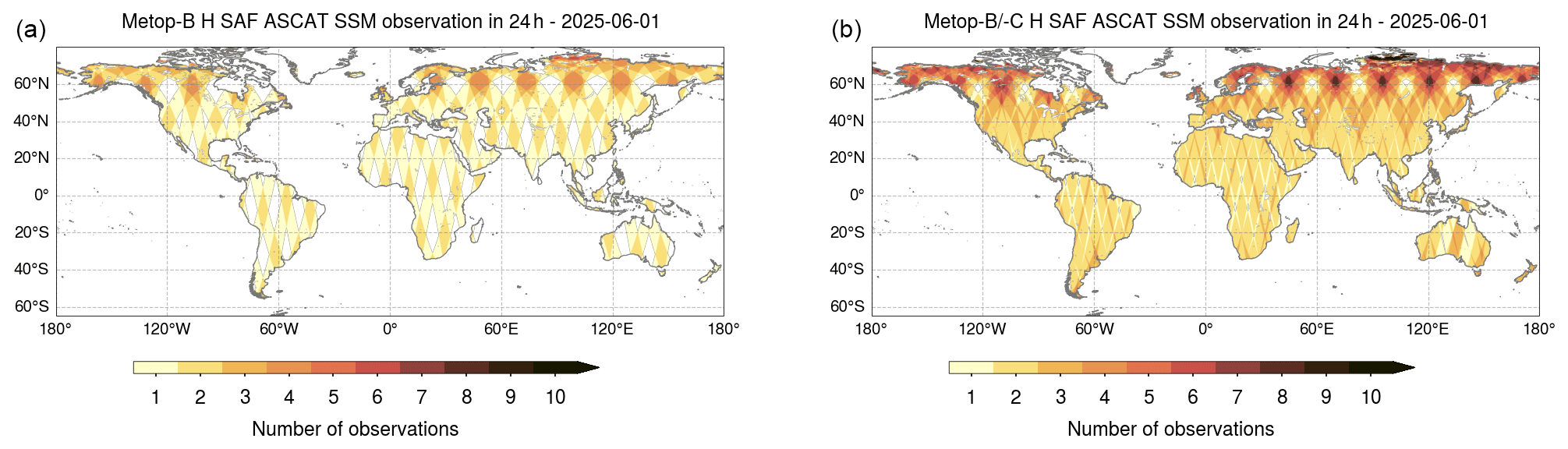
Figure 9ASCAT observations recorded within a 24 h period over land: (a) Metop-B only, (b) combined Metop-B and Metop-C data. ASCAT SSM data © EUMETSAT.
The ascat Python package provides utility functions for converting a collection of swath files into time series format (Hahn et al., 2025). During this process, a satellite identifier variable is added to each observation to preserve information about the source platform. Figure 10 shows an example SSM time series and its rolling average over central Italy. SSM is highly sensitive to atmospheric forcing, including precipitation, evaporation, wind, and solar radiation, and therefore exhibits pronounced short-term variability. SSM anomalies, calculated as deviations from their long-term climatological means, serve as valuable indicator of hydrological extremes or shifts in land surface conditions (see Fig. 10b).
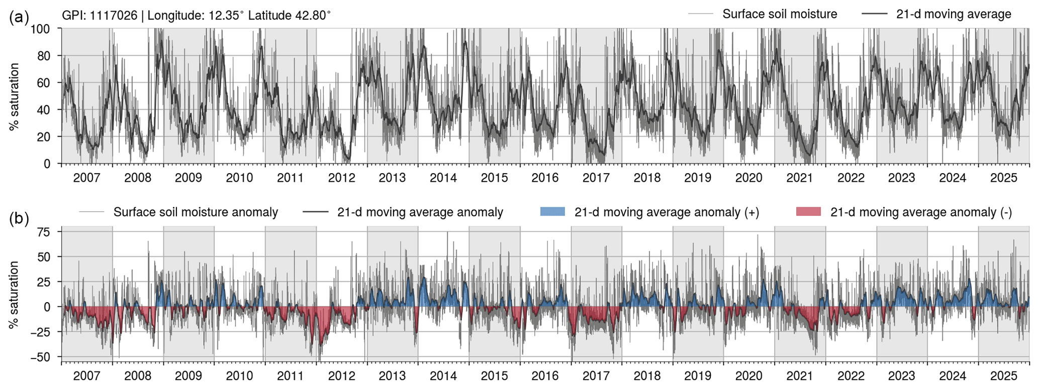
Figure 10Example ASCAT SSM time series for a grid point in central Italy. The top time series (a) shows SSM and a rolling average, while the bottom time series (b) illustrates the anomalies.
4.2 Comparison against ESA CCI Passive SM and Noah GLDAS-2.1
Quality assessment was performed as outlined in Sect. 3.5. The main performance metrics are the Pearson correlation coefficient (R) and Signal-to-Noise Ratio (SNR). The validation covered the time period from 1 January 2007 until 31 December 2023 in case of both reference datasets.
4.2.1 Pearson correlation
Figures 11 and 12 present global maps of Pearson R along with the corresponding number of observation pairs. In case of Pearson R between ASCAT SSM 6.25 km and ESA CCI Passive SM, 17.9 % of grid points are above 0.75 % and 57.8 % are higher than 0.5 (see Fig. 11a). Similar results can be seen for ASCAT SSM 12.5 km as well, with 19.6 % grid points above 0.75 % and 59.2 % higher than 0.5 (see Fig. 11c). In general, lower performance is observed in regions with limited soil moisture variability, such as deserts, as well as at higher latitudes where the soil remains frozen or covered by snow for extended periods and validation is consequently restricted to summer months. In contrast, the best agreement is found in areas with strong seasonal variability, including monsoonal, savanna, Mediterranean, and tropical wet-and-dry climate zones.
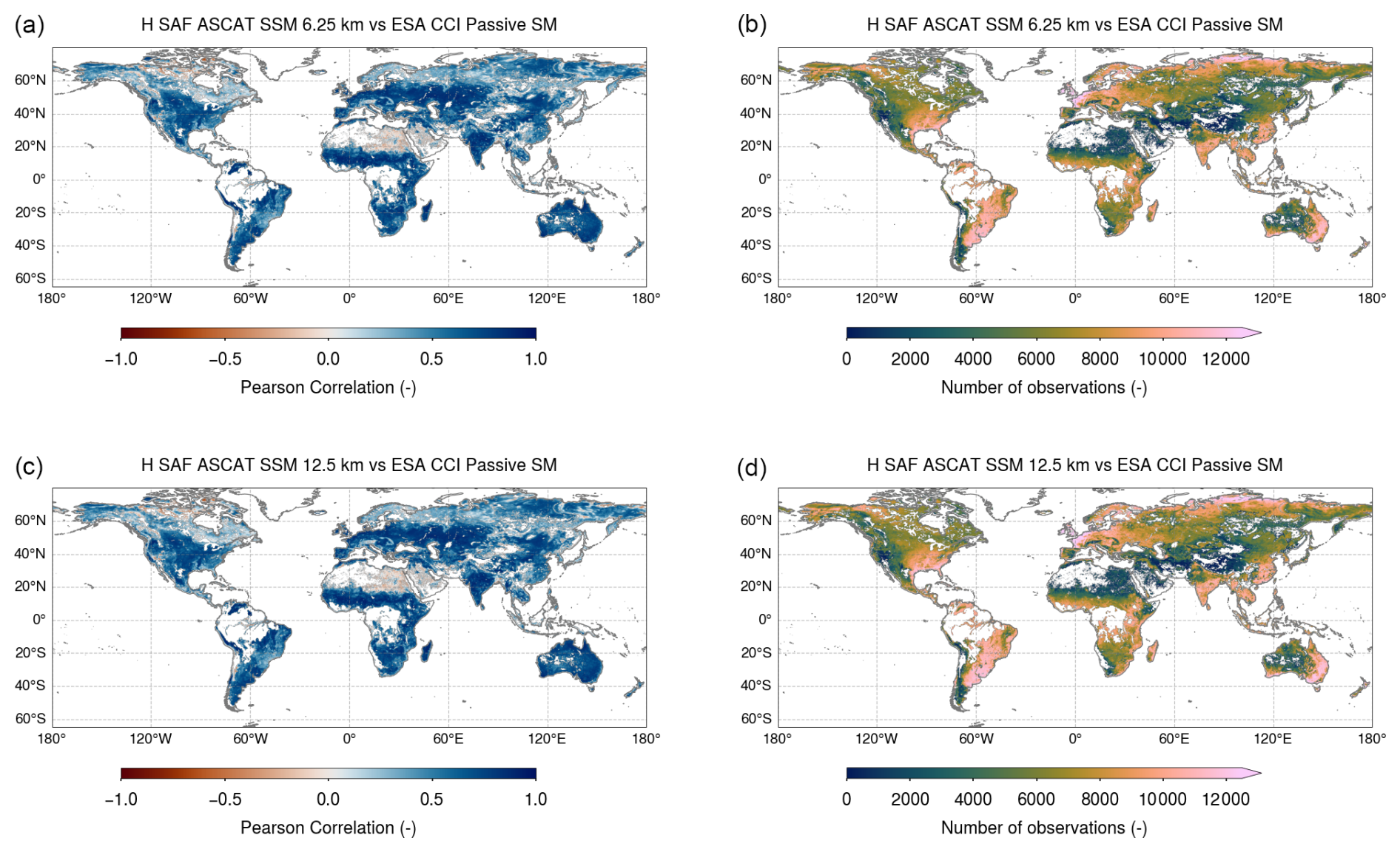
Figure 11Global maps of the Pearson correlation coefficient (a) and the number of observation pairs (b) between ASCAT SSM at 6.25 km and ESA CCI Passive SM are shown in the top half, while corresponding maps for ASCAT SSM at 12.5 km (c, d) are presented in the bottom half. ASCAT SSM data © EUMETSAT. ESA CCI Passive Soil Moisture data © ESA.
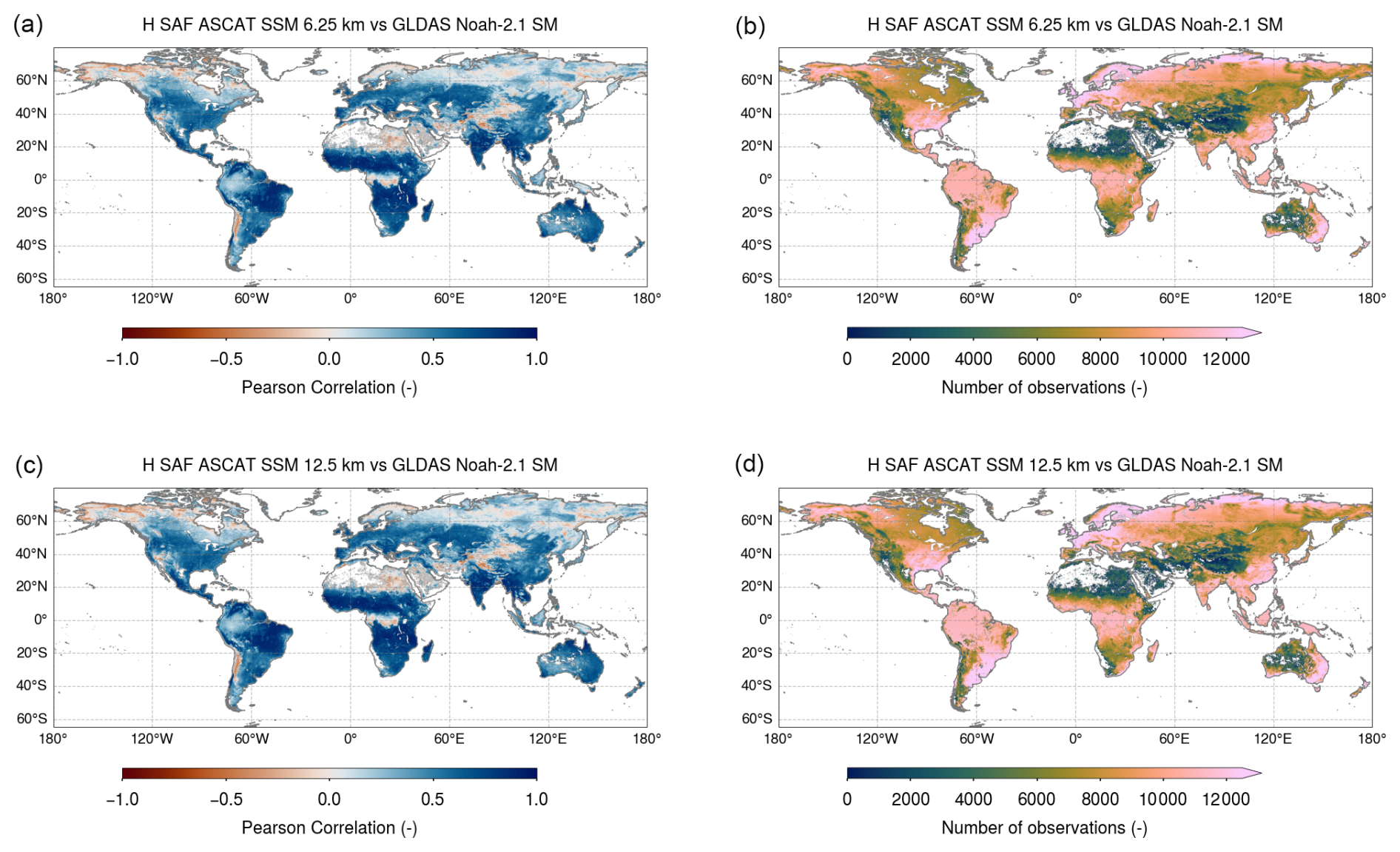
Figure 12Global maps of the Pearson correlation coefficient (a) and the number of observation pairs (b) between ASCAT SSM at 6.25 km and Noah GLDAS-2.1 are shown in the top half, while corresponding maps for ASCAT SSM at 12.5 km (c, d) are presented in the bottom half. ASCAT SSM data © EUMETSAT. GLDAS-2.1 (Noah) data © NASA.
A similar pattern can be seen in the results of Pearson R between ASCAT SSM 6.25 km and Noah GLDAS-2.1 SM with 13.1 % grid points above 0.75 % and 45.9 % higher than 0.5 (see Fig. 12a) and 14.5 % grid points above 0.75 % and 47.7 % higher than 0.5 looking at ASCAT SSM 12.5 km (see Fig. 12c). In comparison to ESA CCI Passive SM, fewer regions have been masked, allowing densely vegetated areas such as the Amazon, Congo, and Indonesian rainforests to be included in the analysis. This reveals the lower performance of the ASCAT SSM datasets in these regions, where dense canopy cover reduces the sensitivity of backscatter signals to soil moisture changes. Notably, these areas could be excluded by applying the soil moisture sensitivity information (< 1 dB) available in the ASCAT SSM datasets (see Table 5).
Figures 11a, c and 12a, c show no significant performance differences of Pearson R between ASCAT SSM 6.25 and 12.5 km. However, there are consistent, albeit small, differences indicating slightly higher Pearson R values for ASCAT SSM 12.5 km. When comparing the Pearson R values (ASCAT SSM 6.25 km minus ASCAT SSM 12.5 km using nearest neighbour grid points), the inter-quartile range (IQR) varies between 0.0 and −0.2 for both ESA CCI Passive SM and Noah GLDAS-2.1. This observed behaviour can be expected since ASCAT SSM 6.25 km is anticipated to exhibit more spatio-temporal fluctuations and noise compared to ASCAT SSM 12.5 km. In fact, the new ASCAT SSM 6.25 km dataset demonstrated a robust performance, even in the absence of globally comparable reference datasets for validation. While direct comparisons against the reference data used for the 12.5 km product is not fully appropriate due to the scale mismatch, the ASCAT SSM 6.25 km product shows a strong agreement. This performance underscores its potential value for applications requiring SSM at higher spatial resolution.
4.2.2 Signal-to-Noise Ratio (SNR)
Figure 13a and c illustrate the Signal-to-Noise Ratio (SNR) computed between the ASCAT SSM datasets, ESA CCI Passive SM and Noah GLDAS-2.1 SM. In case of ASCAT SSM 6.25 km, more than 35.6 % grid points show a SNR higher than 3 dB, while 56.0 % are above 0 dB. Comparing the results against ASCAT SSM 12.5 km shows minor improvements with 38.6 % (SNR > 3 dB) and 58.1 % (SNR > 0 dB), respectively. In contrast to the Pearson R, which may remain high despite substantial noise, the SNR derived from triple collocation analysis (TCA) is a more fundamental metric. It explicitly quantifies the relative contribution of signal and noise, thereby providing a more critical assessment of data quality. This is evident in many regions with low soil moisture variability, where the SNR becomes negative indicating a higher noise variance with respect to the signal component (e.g. desert areas of Africa, the Arabian Peninsula, central Australia, and North America). Similarly, in high-latitude regions where the Pearson R is weakly positive, the SNR becomes negative. As previously mentioned, validation of the full seasonal cycle is not always feasible due to the presence of frozen soils or persistent snow cover. This limitation poses a challenge for a comprehensive validation and interpretation. Therefore, a negative SNR should not be interpreted as evidence that the ASCAT SSM datasets are unusable in these regions. Instead, it signals challenges arising from environmental factors. Users are always advised to take local conditions into account when interpreting remote sensing soil moisture datasets.
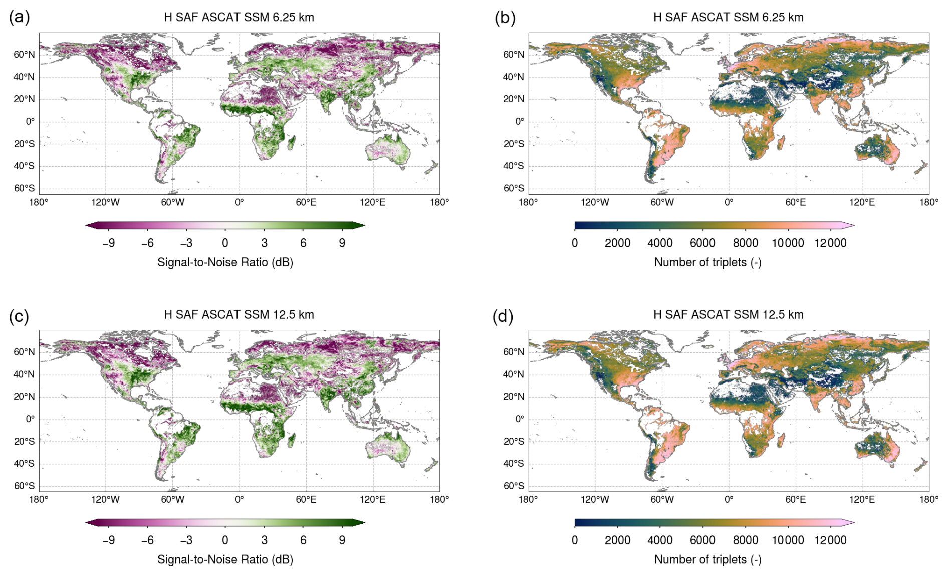
Figure 13Global maps of SNR (a) and the number of triplets (b) between H SAF ASCAT SSM 6.25 km, Noah GLDAS-2.1 and ESA CCI Passive SM are shown in the top half, while corresponding maps for H SAF ASCAT SSM 12.5 km (c, d) are presented in the bottom half. H SAF ASCAT SSM data © EUMETSAT. GLDAS-2.1 (Noah) data © NASA. ESA CCI Passive Soil Moisture data © ESA.
Based on the SNR performance evaluation, there is no significant difference between ASCAT SSM 6.25 and 12.5 km datasets (see Fig. 13a, c). However, a point-wise comparison of SNR (ASCAT SSM 6.25 km minus ASCAT SSM 12.5 km using nearest neighbour grid points) reveals that the inter-quartile range (IQR) varies between 0.3 and −0.6 dB. As discussed for Pearson R, a slightly better performance can be anticipated due to higher spatio-temporal frequencies in ASCAT SSM 6.25 km compared to ASCAT SSM 12.5 km. Overall, these small SNR differences confirm that the higher-resolution ASCAT SSM 6.25 km dataset does not introduce substantial noise.
4.3 Comparison against ISMN
A total of 43 in-situ networks from the International Soil Moisture Network (ISMN) that temporally overlap with the ASCAT SSM datasets were used for validation (Table B1). For each network, sensors measuring within the 0–10 cm depth range were primarily selected. Figure 14 shows boxplots of the Pearson R for each network comparing the ASCAT SSM datasets against to each other. The number of sensors per network is shown next to the network name.
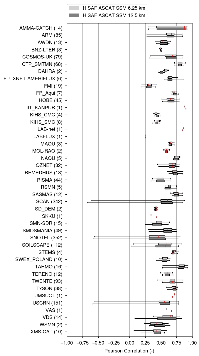
Figure 14Pearson R computed between H SAF ASCAT SSM (6.25 and 12.5 km) and 43 ISMN in-situ networks. The evaluation was performed on data ranging from January 2007 to December 2024. The boxplots depict the distribution of Pearson R for each network, with the number of sensors next to the network name. Whiskers extend to the 2nd and 98th percentiles of the Pearson R distribution per network.
The inter-quartile range (IQR) of the boxplots lies between the interval 0.25 and 0.85, with over two-thirds of the networks indicating a 25th percentile (lower bound of the IQR) above 0.5. The highest performance of the ASCAT SSM datasets is observed for the networks CTP_SMTMN, NAQU, REMEDHUS, SASMAS, and THAMO. In contrast, 24 sensors from three networks (SCAN, SNOTEL, and USCRN) yield negative Pearson R values. All of these sensors are located in the United States (California, Nevada, and Utah), with more than 90 % situated at elevations above 2000 m. The combination of arid climate, limited signal variability, complex topography and the presence of (undetected) subsurface scattering effects likely explains the reduced performance in these regions.
While the overall distributions of Pearson R values remain similar for both ASCAT SSM datasets, their median values show minor network-specific variations. Specifically, the ASCAT SSM 6.25 km dataset shows slightly higher medians for DAHRA, RISMA, and SNOTEL, whereas the 12.5 km dataset performs marginally better for SCAN, USCRN, and WSMN. Neither resolution consistently outperforms the other and the differences observed are small in magnitude.
A comparison of our Pearson R evaluation between the ASCAT SSM datasets and the ISMN networks with previous studies based on earlier versions of ASCAT SSM datasets indicates generally consistent performance (e.g., Fascetti et al., 2016; Al-Yaari et al., 2019; Beck et al., 2021; Mazzariello et al., 2023). However, a direct comparison of results remains challenging due to differences in the input datasets, applied pre-processing steps and overall validation setup.
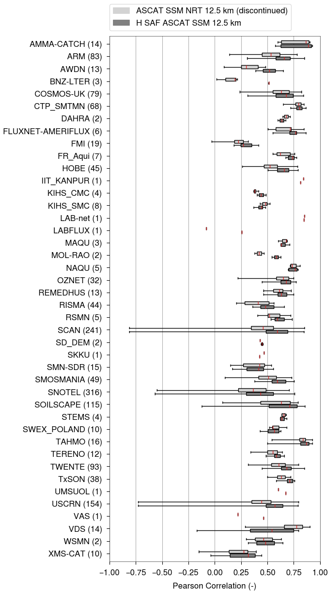
Figure 15Pearson R computed for the discontinued ASCAT SSM NRT 12.5 km dataset and the new H SAF ASCAT SSM 12.5 km dataset against 42 ISMN in-situ networks (SASMAS network is missing since it is not overlapping with the evaluation period). The evaluation was performed on data ranging from January 2008 to December 2023. The boxplots depict the distribution of Pearson R for each network, with the number of sensors next to the network name. Whiskers extend to the 2nd and 98th percentiles of the Pearson R distribution per network.
In addition, a comparison between the discontinued ASCAT SSM NRT 12.5 km dataset and the new ASCAT SSM 12.5 km dataset has been performed for the time period January 2008 until December 2023. In this case, no subsurface scattering masking has been applied, since it has been missing for the discontinued ASCAT SSM NRT 12.5 km dataset. Figure 15 shows the distribution of Pearson R for each network comparing the two datasets against ISMN. The new ASCAT SSM 12.5 km dataset shows better or equal results for the majority of ISMN networks.
The largest in-situ networks are located in the U.S. (SCAN, SNOTEL, SOILSCAPE, USCRN), which cover a variety of climate regions. The IQR and whisker extents of their boxplots indicate a mixture of results, reflecting the different soil moisture dynamics across these regions. As noted previously, limited signal variability and subsurface scattering effects in arid regions, as well as in-situ stations at higher altitudes collectively result in poor performance, reflected in the lower whisker ends. Nonetheless, these networks show a clear overall improvement for the new ASCAT SSM 12.5 km dataset. In-situ networks distributed over Europe (e.g. COSMOS-UK, HOBE, REMEDHUS, RSMN, TWENTE, TERENO), also indicate a better performance compared to the discontinued ASCAT SSM NRT 12.5 km dataset. As shown by Hahn et al. (2021), the spatially variable vegetation correction plays an important role in improving results across North America and Europe, which can also be seen in this validation.
In-situ networks where ASCAT SSM generally performs poorly include e.g. FMI, LABFLUX and XMS-CAT. The Finnish Meteorological Institute (FMI) stations are located in Sodankylä, an Arctic research station in northern Finland. Due to winter frost conditions, validation is limited to summer months. Combined with the surrounding boreal forest canopy, leading to a loss of sensitivity to soil moisture changes, makes it an overall challenging environment. In case of LABFLUX and XMS-CAT, both sites are located in areas with complex topography. LABFLUX in north-west Italy near the Alps, and XMS-CAT in north-east Spain near the Pyrenees. As discussed in Sect. 3.4.2, rough terrain is a known challenge for active microwave soil moisture retrieval, as it introduces backscatter signal distortions arising from varying viewing geometries and distinct echo responses. Even though results are looking better for the latest ASCAT SSM 12.5 km dataset, topographic complexity continues to limit performance gains.
Only a small number of networks (DAHRA, IIT_KANPUR, KIHS_SMC, VDS) indicate a reverse performance trend, with VDS showing the largest differences. The VDS network was operational from June 2017 to February 2021 and is situated in southern Myanmar, a region dominated by irrigated and rainfed rice cultivation. Backscatter signal characteristics over rice fields are inherently complex, as the alternating flooded and non-flooded surface states have distinct scattering regimes. Consequently, changes in the backscatter-incidence angle relationship reflects not only vegetation phenology but also scattering mechanisms associated with open water surfaces and partially submerged vegetation. As discussed in Hahn et al. (2021), the updated vegetation correction applied in the ASCAT SSM NRT 12.5 km dataset may amplify signal contributions unrelated to soil moisture, thereby reducing retrieval performance compared to the discontinued ASCAT SSM NRT 12.5 km dataset. However, the fundamental issue is not the vegetation parameterisation itself, but rather the occurrence of time periods where backscatter variations are no longer dominated by soil moisture changes. During such periods, reliable soil moisture retrieval is no longer possible and these observations must be masked. In case of temporarily flooded surfaces, no such masking exists and scattering characteristics that change the typical incidence angle dependent signal dynamics of vegetation influence the vegetation correction and thereby compromise the soil moisture retrieval.
The H SAF ASCAT SSM datasets are available globally (180° W 65° S–180° E 80° N) in netCDF swath file format (6.25 km sampling: https://doi.org/10.15770/EUM_SAF_H_0012, H SAF, 2025c, and 12.5 km sampling: https://doi.org/10.15770/EUM_SAF_H_0011, H SAF, 2025a) (H SAF, 2025b, d, e, f). Soil moisture is expressed in degree of saturation (0 % dry soil, 100 % saturated soil) representing the topmost soil layer (< 5 cm). Advisory flags are included to give context on soil state, land cover, and scattering behaviour. Users are encouraged to apply these flags to exclude time periods or locations influenced by frozen soil or snow cover prior to data usage. When available, external datasets on soil temperature and snow cover should also be used to refine this filtering.
This article introduces the first ASCAT SSM dataset produced at a nominal sampling of 6.25 km, alongside the standard 12.5 km sampling commonly used in previous ASCAT SSM dataset versions (H SAF, 2017, 2020a, 2021a). The ASCAT SSM datasets are available as near real-time (NRT), climate data record (CDR), and interim climate data record (ICDR) products and distributed through the H SAF online archive via FTP. The ICDR serves as an extension of the CDR, generated using the same processing chain and input data, while the NRT product priorities timeliness over long-term consistency. ASCAT SSM NRT products are additionally distributed via EUMETCast, a satellite-based broadcast system operated by EUMETSAT.
Both ASCAT SSM datasets presented in this article are generated from ASCAT Level 1B SZF backscatter data using the same semi-empirical change detection algorithm. They differ only in the spatial resampling radius. During the resampling process, backscatter echos over surfaces not sensitive to soil moisture changes (e.g., open water, urban areas) are masked. This masking, combined with the smaller resampling radius of the ASCAT SSM 6.25 km dataset (14 km vs. 24 km), increases the likelihood of reduced or insufficient echo counts, potentially leading to higher noise or, in extreme cases, discontinuities in data coverage. At the same time, the finer spatial resolution of the 6.25 km dataset introduces greater spatio-temporal signal variability. Despite all these effects, global validation against Noah GLDAS-2.1 and ESA CCI Passive v09.1, along with comparisons to 43 ISMN in-situ networks, demonstrates that the ASCAT SSM 6.25 km dataset achieves a Pearson R and SNR performance equivalent to that of the standard 12.5 km product. Minor, yet consistent, differences were observed in the global validation, which are small and expected given that the reference datasets do not share the same spatial resolution as the ASCAT SSM 6.25 km product.
Overall, the validation results indicate best performance of ASCAT SSM in regions with strong seasonal variability, including monsoonal, savanna, Mediterranean, and tropical wet-and-dry zones. In contrast, a lower performance can be found in areas characterised by limited soil moisture variability (e.g., deserts), dense vegetation, pronounced topographic complexity, wetlands, or higher latitudes (> 60° N). Degradation in these regions is driven by distinct mechanisms. Limited soil moisture variability in arid regions reduces the signal dynamic range, undermining the statistical robustness. Dense vegetation attenuates the microwave signal through canopy absorption and volume scattering, effectively masking soil surface conditions. Pronounced topographic complexity introduces heterogeneous scattering patterns that overlay with soil moisture contributions. Large wetlands with standing water either generate strong specular reflection or further complicate the backscatter signal response by emergent vegetation that creates more complex scattering effects. Finally, higher latitudes experience longer periods of frozen soil and snow cover, which disrupts the physical relationship between microwave backscatter and liquid soil moisture, making the signal insensitive or misleading. Thus, the change detection algorithm used to derived the ASCAT SSM datasets performs optimally under conditions of: (i) low to moderate vegetation density, (ii) unfrozen and snow-free terrain, (iii) negligible subsurface scattering, (iv) low to moderate topographic complexity, (v) absence of wetlands, and (vi) absence of radio frequency interference (RFI).
The Metop-Second Generation (Metop-SG) B-series satellites (Metop-SG B1 scheduled for launch in October 2026), will carry the next-generation scatterometer (SCA). Sharing an instrument design similar to ASCAT, SCA will enable a seamless continuity of soil moisture datasets. Furthermore, SCA features key enhancements over ASCAT including an improved radiometric resolution and an additional VH- and HH-channel on both left and right Mid beams. These upgrades create new opportunities to refine the soil moisture retrieval algorithm. Finally, and most importantly, operational continuity from ASCAT to SCA, combined with cross-calibration against the ERS-1 and ERS-2 missions, will establish a unique, multi-decade dataset essential for global climate change research.
A1 Azimuth angle dependency of backscatter
Azimuth angle dependency of backscatter is very common over land and can be particularly pronounced in mountainous areas or sandy deserts (Stephen and Long, 2002). The anisotropic nature of a target is closely related to the satellite's orbit and the instrument's geometry. A backscatter signal bias caused by azimuthal modulation can significantly affect the retrieval of geophysical parameters, such as soil moisture.
Similar to Bartalis et al. (2006a), an empirical approach is used to derive statistically expected values for a combination of observation geometries, which in the end normalises σ0 observations with respect to the azimuth angle. The azimuth angle is determined by the beam (Fore, Mid, or Aft), the swath position (left or right), and the orbit direction (ascending or descending), resulting in twelve distinct azimuth configurations (ϕi, where ) for ASCAT. For each azimuth configuration, the dependency of backscatter on the incidence angle is modelled using a second-order polynomial estimating the coefficients .
Additionally, a reference model (i=13) is fitted to all observations combined. This results in a total of coefficients. The differences between the polynomial coefficients of the twelve individual acquisition geometries and the reference model (i=13) are used to derive new polynomial coefficients, which are then used to compute corrections applied to the backscatter observation. In this way, the individual observation configuration are adjusted to a common reference, effectively eliminating static azimuth angle effects.
where represents the corrected backscatter for each configuration i. All following processing steps are using the azimuth angle corrected backscatter, but for simplicity we use the usual notation of backscatter σ0 rather than the hat notation .
A2 Estimated standard deviation of backscatter
The Estimated Standard Deviation (ESD) quantifies the standard deviation of backscatter (expressed in dB) and serves as a measure of noise. Computing the ESD represents the initial step in error propagation. It is derived from the Fore and Aft beam measurements (, ) based on the following assumption: all three beams observe the same target, and the Fore and Aft beams share identical incidence angles due to the instrument observation geometry. Consequently, in the absence of azimuth angle dependency of backscatter, the measurements from the Fore and Aft beams should be comparable, meaning they are statistically instances of the same distribution. Therefore, the expected value of their difference
should be zero, and its variance should be twice the variance of one of the beams (i.e Var[δ]=2Var[σ0]). This can be derived using error propagation and neglecting higher order terms. Hence, the ESD is defined as
A3 Incidence angle dependency of backscatter
Over land surfaces, backscatter generally decreases with increasing incidence angle, a relationship that is often approximated by a linear function in the decibel (dB) domain. However, at larger incidence angles, significant contributions from volume scattering can cause the backscatter signal to increase, leading to deviations from the linear relationship (see Fig. A1) (Wagner et al., 2013). To account for these higher-order variations, a second-order function provides a more accurate representation of the incidence angle dependence. A well-calibrated model of the incidence angle dependence of backscatter has two key objectives. First, it allows interpolating backscatter observations across different incidence angles, e.g. interpolating all observations to a common reference incidence angle. Second, changes of the incidence angle behaviour can reveal valuable information about surface characteristics and underlying geophysical parameters.
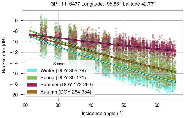
Figure A1Backscatter variation with incidence angle over agricultural land in northwest Iowa, USA.
In this case, a second-order Taylor polynomial is used to model the incidence angle dependence of backscatter. The model represents a finite sum of the function's first and second derivative with the incidence angle of 40° serving as the expansion point.
The first derivative, σ′ (dB degree−1), and the second derivative, σ′′ (dB degree−2), are referred to as the slope and curvature, respectively. Once these parameters are estimated, the Taylor polynomial expansion can be used to approximate the backscatter in the vicinity of the chosen expansion point. This approach allows for the interpolation of backscatter observations from their original incidence angles to a common reference incidence angle. At the reference incidence angle, backscatter observations can be directly compared, as the dependency on incidence angle has been effectively eliminated.
The estimation of σ′ and σ′′ is based on the computation of the local slope (see Eq. A6) using the Fore, Mid, Aft beam backscatter observations (, , ), which provides an instantaneous characterisation of the incidence angle dependence of the backscatter signal. Since the Mid beam incidence angle (θm) is separated by approximately 9° compared to the Fore and Aft beam incidence angle (θf, θa) two local slope values can be obtained from a backscatter triplet (, ). Typically a larger number of Fore-Mid and Aft-Mid beam observations are required to capture a sufficiently wide range of incidence angles. Ultimately, σ′ and σ′′ are estimated through a weighted local linear regression performed for each day of the year (Melzer, 2013). A detailed description of the methodology can be found in Hahn et al. (2017). It is based on a Kernel Smoother (KS) approach using the Epanechnikov kernel to weigh observations based on their temporal distance from the target day. A kernel bandwidth of λ=21 d is used, which corresponds to a symmetric smoothing window of 42 d.
Depending on the number of years included in the computation, the estimates of σ′ and σ′′ may represent either a multi-year climatology or a year-specific time series. Although a year-specific time series would allow for the assessment of inter-annual variability, a multi-year climatology is currently used to ensure greater robustness and suitability for near real-time applications (Steele-Dunne et al., 2019, 2021).
A4 Interpolation to reference incidence angle
The slope and curvature parameters are calculated for each day of the year (DOY) and used in the Taylor polynomial to interpolate backscatter observations to a common reference incidence angle of 40°. This angle is selected to be close to the centre of the observed incidence angle range to minimise interpolation errors. The interpolation is performed independently for each beam (b) (see Eq. A7), and the resulting values are averaged across all three beams at 40° to further reduce noise (see Eq. A8).
A4.1 Error propagation
The Estimated Standard Deviation of backscatter (ESD[σ0]) serves as the basis for error propagation (see Sect. A2). These backscatter uncertainties are carried forward to the variances of the estimated slope and curvature parameters (Var[σ′], Var[σ′′]), which are derived under the assumption that all local slope values exhibit identical, uncorrelated variances, as described by Hahn et al. (2017). The variance of the local slopes is estimated from the residuals of the weighted local linear regression, which is performed using the Epanechnikov kernel. All of these error estimates are subsequently propagated to quantify the uncertainty of the backscatter values interpolated to the reference incidence angle of 40°:
Upon averaging for each beam, the noise variance becomes:
Although error propagation is applied when converting backscatter observations to the dry and wet cross-over angles, the resulting propagated errors are not directly used. This is because the dry and wet backscatter references are derived from percentiles of the backscatter distributions rather than from individual measurements. As a result, the associated variances (, ) cannot be explicitly calculated through standard error propagation and are therefore not accounted for in this step. However, error propagation formulas are explicitly applied during the conversion of the dry and wet backscatter references to the common reference incidence angle of 40°. In this case, the total noise is computed using the following expressions:
where the terms and are unknown and set to zero. Hence, the total error is governed solely by the uncertainties in the slope and curvature parameters when interpolating the dry and wet reference to 40°.
By proceeding with the error propagation, the resulting uncertainty in soil moisture can be expressed as follows:
with
It is worth noting that the error model employed is not designed to capture error sources arising under conditions such as frozen soil, snow cover, subsurface scattering, or wetlands. In these environments, the backscatter signal is influenced by factors other than soil moisture, and as such, both noise estimation and soil moisture retrieval may be compromised.
A4.2 Wet correction
In some regions, truly saturated soil conditions are rarely or never observed due to prevailing climatic factors. Therefore, a correction must be applied to simulate wet conditions and obtain a more realistic wet reference. This wet correction relies on an external climate dataset (Peel et al., 2007), as scatterometer measurements alone are insufficient to reliably identify such regions. The correction is implemented in two steps: (i) first the lower limit of the wet reference is set to at least −10 dB and (ii) regions where saturated soil moisture conditions are rarely encountered (Köppen Geiger climate class B), values are raised until the sensitivity (defined as ) reaches a minimum of 5 dB (Naeimi et al., 2009b).
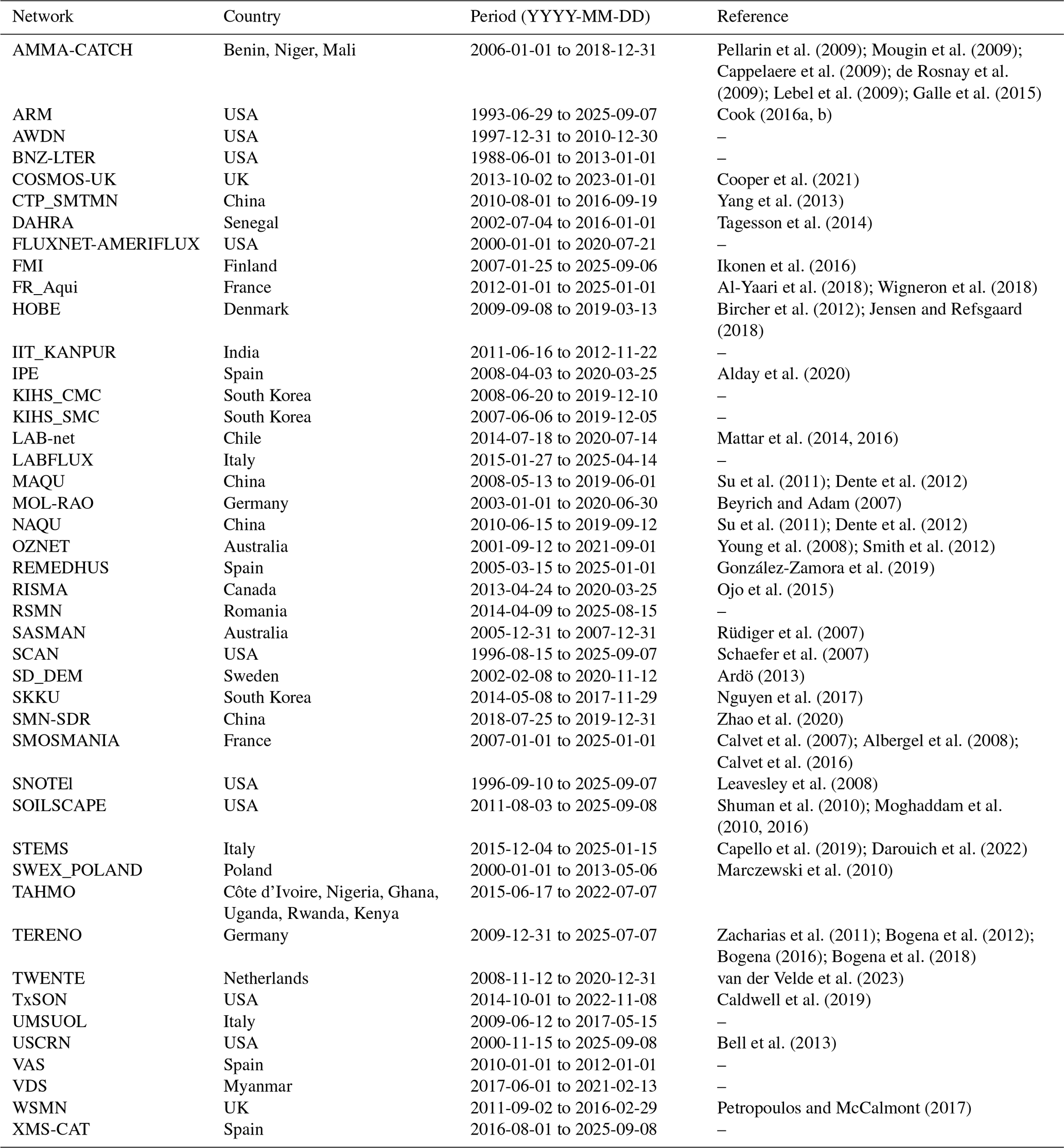
Sebastian Hahn: Writing, Software development, Processing, Validation, Visualization. Thomas Melzer: Writing – review & editing, Error characterisation, Backscatter-incidence angle characterisation. Wolfgang Wagner: Writing – review & editing, Original algorithm development, Supervision.
The contact author has declared that none of the authors has any competing interests.
Publisher's note: Copernicus Publications remains neutral with regard to jurisdictional claims made in the text, published maps, institutional affiliations, or any other geographical representation in this paper. The authors bear the ultimate responsibility for providing appropriate place names. Views expressed in the text are those of the authors and do not necessarily reflect the views of the publisher.
The development of the H SAF ASCAT SSM datasets was carried out in the framework of the forth SAF Continuous Development and Operations Phase (CDOP 4) of the EUMETSAT Satellite Application Facility on Support to Operational Hydrology and Water Management (H SAF). We thank EUMETSAT and all H SAF consortium members for their continuous support.
This paper was edited by Han Ma and reviewed by three anonymous referees.
Aires, F., Weston, P., Rosnay, P., and Fairbairn, D.: Statistical approaches to assimilate ASCAT soil moisture information-I. Methodologies and first assessment, Q. J. Roy. Meteor. Soc., 147, 1823–1852, https://doi.org/10.1002/qj.3997, 2021. a
Al-Yaari, A., Dayau, S., Chipeaux, C., Aluome, C., Kruszewski, A., Loustau, D., and Wigneron, J.-P.: The AQUI Soil Moisture Network for Satellite Microwave Remote Sensing Validation in South-Western France, Remote Sens., 10, 1839, https://doi.org/10.3390/rs10111839, 2018. a
Al-Yaari, A., Wigneron, J.-P., Dorigo, W., Colliander, A., Pellarin, T., Hahn, S., Mialon, A., Richaume, P., Fernandez-Moran, R., Fan, L., Kerr, Y., and Lannoy, G. D.: Assessment and inter-comparison of recently developed/reprocessed microwave satellite soil moisture products using ISMN ground-based measurements, Remote Sens. Environ., 224, 289–303, https://doi.org/10.1016/j.rse.2019.02.008, 2019. a, b
Albergel, C., Rüdiger, C., Pellarin, T., Calvet, J.-C., Fritz, N., Froissard, F., Suquia, D., Petitpa, A., Piguet, B., and Martin, E.: From near-surface to root-zone soil moisture using an exponential filter: an assessment of the method based on in-situ observations and model simulations, Hydrol. Earth Syst. Sci., 12, 1323–1337, https://doi.org/10.5194/hess-12-1323-2008, 2008. a
Alday, J. G., Camarero, J. J., Revilla, J., and Resco de Dios, V.: Similar diurnal, seasonal and annual rhythms in radial root expansion across two coexisting Mediterranean oak species, Tree Physiol., 40, 956–968, https://doi.org/10.1093/treephys/tpaa041, 2020. a
Anderson, C., Bonekamp, H., Duff, C., Figa-Saldana, J., and Wilson, J. J. W.: Analysis of ASCAT Ocean Backscatter Measurement Noise, IEEE T. Geosci. Remote, 50, 2449–2457, https://doi.org/10.1109/TGRS.2012.2190739, 2012a. a
Anderson, C., Figa, J., Bonekamp, H., Wilson, J. J. W., Verspeek, J., Stoffelen, A., and Portabella, M.: Validation of Backscatter Measurements from the Advanced Scatterometer on MetOp-A, J. Atmos. Ocean. Tech.y, 29, 77–88, https://doi.org/10.1175/JTECH-D-11-00020.1, 2012b. a
Ardö, J.: A 10-Year Dataset of Basic Meteorology and Soil Properties in Central Sudan, Dataset Papers Geosci., 2013, 1–6, https://doi.org/10.7167/2013/297973, 2013. a
AWST, TU Wien, and CESBIO: QA4SM Software User Manual, Version 3.1, Tech. rep., QA4SM Consortium, 2025. a
Bartalis, Z., Kidd, R. A., and Scipal, K.: Development and Implementation of a Discrete Global Grid System for Soil Moisture Retrieval Using the MetOp ASCAT Scatterometer, in: First EPS/MetOp RAO Workshop, Frascati, Italy, 15–17 May, eSA Special Publication SP-618, 2006a. a
Bartalis, Z., Scipal, K., and Wagner, W.: Azimuthal Anisotropy of Scatterometer Measurements over Land, IEEE T. Geosci. Remote, 44, 2083–2092, 2006b. a
Bartalis, Z., Wagner, W., Naeimi, V., Hasenauer, S., Scipal, K., Bonekamp, H., Figa, J., and Anderson, C.: Initial soil moisture retrievals from the METOP-A Advanced Scatterometer (ASCAT), Geophys. Res. Lett., 34, https://doi.org/10.1029/2007gl031088, 2007. a
Bauer-Marschallinger, B., Paulik, C., Hochstöger, S., Mistelbauer, T., Modanesi, S., Ciabatta, L., Massari, C., Brocca, L., and Wagner, W.: Soil Moisture from Fusion of Scatterometer and SAR: Closing the Scale Gap with Temporal Filtering, Remote Sens., 10, 1030, https://doi.org/10.3390/rs10071030, 2018. a
Beaudoing, H., Rodell, M., and NASA/GSFC/HSL: GLDAS Noah Land Surface Model L4 3 hourly 0.25 x 0.25 degree, Version 2.1, Goddard Earth Sciences Data and Information Services Center (GES DISC) [data set], https://doi.org/10.5067/E7TYRXPJKWOQ, 2020. a
Beck, H. E., Pan, M., Miralles, D. G., Reichle, R. H., Dorigo, W. A., Hahn, S., Sheffield, J., Karthikeyan, L., Balsamo, G., Parinussa, R. M., van Dijk, A. I. J. M., Du, J., Kimball, J. S., Vergopolan, N., and Wood, E. F.: Evaluation of 18 satellite- and model-based soil moisture products using in situ measurements from 826 sensors, Hydrol. Earth Syst. Sci., 25, 17–40, https://doi.org/10.5194/hess-25-17-2021, 2021. a, b
Bell, J. E., Palecki, M. A., Baker, C. B., Collins, W. G., Lawrimore, J. H., Leeper, R. D., Hall, M. E., Kochendorfer, J., Meyers, T. P., Wilson, T., and Diamond, H. J.: U.S. Climate Reference Network Soil Moisture and Temperature Observations, J. Hydrometeorol., 14, 977–988, https://doi.org/10.1175/jhm-d-12-0146.1, 2013. a
Beyrich, F. and Adam, W.: Site and Data Report for the Lindenberg Reference Site in CEOP – Phase 1, Tech. Rep. 230, Deutscher Wetterdienst, Offenbach am Main, 2007. a
Bircher, S., Balling, J. E., Skou, N., and Kerr, Y. H.: Validation of SMOS Brightness Temperatures During the HOBE Airborne Campaign, Western Denmark, IEEE T. Geosci. Remote, 50, 1468–1482, https://doi.org/10.1109/TGRS.2011.2170177, 2012. a
Bogena, H., Kunkel, R., Puetz, T., Vereecken, H., Krueger, E., Zacharias, S., Dietrich, P., Wollschlaeger, U., Kunstmann, H., and Papen, H.: Tereno-long-term monitoring network for terrestrial environmental research, Hydrol. Wasserbewirts., 56, 138–143, 2012. a
Bogena, H., Montzka, C., Huisman, J., Graf, A., Schmidt, M., Stockinger, M., von Hebel, C., Hendricks-Franssen, H., van der Kruk, J., Tappe, W., Lücke, A., Baatz, R., Bol, R., Groh, J., Pütz, T., Jakobi, J., Kunkel, R., Sorg, J., and Vereecken, H.: The TERENO‐Rur Hydrological Observatory: A Multiscale Multi‐Compartment Research Platform for the Advancement of Hydrological Science, Vadose Zone J., 17, 1–22, https://doi.org/10.2136/vzj2018.03.0055, 2018. a
Bogena, H. R.: TERENO: German network of terrestrial environmental observatories, Journal of Large-Scale Research Facilities JLSRF, 2, A52, https://doi.org/10.17815/jlsrf-2-98, 2016. a
Brocca, L., Melone, F., Moramarco, T., Wagner, W., Naeimi, V., Bartalis, Z., and Hasenauer, S.: Improving runoff prediction through the assimilation of the ASCAT soil moisture product, Hydrol. Earth Syst. Sci., 14, 1881–1893, https://doi.org/10.5194/hess-14-1881-2010, 2010. a
Brocca, L., Moramarco, T., Melone, F., Wagner, W., Hasenauer, S., and Hahn, S.: Assimilation of Surface- and Root-Zone ASCAT Soil Moisture Products Into Rainfall-Runoff Modeling, IEEE T. Geosci. Remote, 50, 2542–2555, https://doi.org/10.1109/TGRS.2011.2177468, 2012. a
Brocca, L., Moramarco, T., Melone, F., and Wagner, W.: A New Method for Rainfall Estimation through Soil Moisture Observations: RAINFALL FROM SOIL MOISTURE OBSERVATIONS, Geophys. Res. Lett., 40, 853–858, https://doi.org/10.1002/grl.50173, 2013. a
Brocca, L., Ciabatta, L., Massari, C., Moramarco, T., Hahn, S., Hasenauer, S., Kidd, R., Dorigo, W., Wagner, W., and Levizzani, V.: Soil as a Natural Rain Gauge: Estimating Global Rainfall from Satellite Soil Moisture Data: Using the Soil as a Natural Raingauge, J. Geophys. Res.-Atmos., 119, 5128–5141, https://doi.org/10.1002/2014JD021489, 2014. a
Brocca, L., Crow, W. T., Ciabatta, L., Massari, C., de Rosnay, P., Enenkel, M., Hahn, S., Amarnath, G., Camici, S., Tarpanelli, A., and Wagner, W.: A Review of the Applications of ASCAT Soil Moisture Products, IEEE J. Sel. Top. Appl. Earth Obs., 10, 2285–2306, https://doi.org/10.1109/JSTARS.2017.2651140, 2017. a
Brocca, L., Filippucci, P., Hahn, S., Ciabatta, L., Massari, C., Camici, S., Schüller, L., Bojkov, B., and Wagner, W.: SM2RAIN–ASCAT (2007–2018): global daily satellite rainfall data from ASCAT soil moisture observations, Earth Syst. Sci. Data, 11, 1583–1601, https://doi.org/10.5194/essd-11-1583-2019, 2019. a
Caldwell, T. G., Bongiovanni, T., Cosh, M. H., Jackson, T. J., Colliander, A., Abolt, C. J., Casteel, R., Larson, T., Scanlon, B. R., and Young, M. H.: The Texas Soil Observation Network:A Comprehensive Soil Moisture Dataset for Remote Sensing and Land Surface Model Validation, Vadose Zone J., 18, 1–20, https://doi.org/10.2136/vzj2019.04.0034, 2019. a
Calvet, J.-C., Fritz, N., Froissard, F., Suquia, D., Petitpa, A., and Piguet, B.: In situ soil moisture observations for the CAL/VAL of SMOS: the SMOSMANIA network, in: 2007 IEEE International Geoscience and Remote Sensing Symposium, IEEE, 1196–1199, https://doi.org/10.1109/igarss.2007.4423019, 2007. a
Calvet, J.-C., Fritz, N., Berne, C., Piguet, B., Maurel, W., and Meurey, C.: Deriving pedotransfer functions for soil quartz fraction in southern France from reverse modeling, SOIL, 2, 615–629, https://doi.org/10.5194/soil-2-615-2016, 2016. a
Capello, G., Biddoccu, M., Ferraris, S., and Cavallo, E.: Effects of Tractor Passes on Hydrological and Soil Erosion Processes in Tilled and Grassed Vineyards, Water, 11, 2118, https://doi.org/10.3390/w11102118, 2019. a
Cappelaere, B., Descroix, L., Lebel, T., Boulain, N., Ramier, D., Laurent, J.-P., Favreau, G., Boubkraoui, S., Boucher, M., Bouzou Moussa, I., Chaffard, V., Hiernaux, P., Issoufou, H., Le Breton, E., Mamadou, I., Nazoumou, Y., Oi, M., Ottlé, C., and Quantin, G.: The AMMA-CATCH experiment in the cultivated Sahelian area of south-west Niger – Investigating water cycle response to a fluctuating climate and changing environment, J. Hydrol., 375, 34–51, https://doi.org/10.1016/j.jhydrol.2009.06.021, 2009. a
Chan, S., Bindlish, R., O’Neill, P., Jackson, T., Njoku, E., Dunbar, S., Chaubell, J., Piepmeier, J., Yueh, S., Entekhabi, D., Colliander, A., Chen, F., Cosh, M., Caldwell, T., Walker, J., Berg, A., McNairn, H., Thibeault, M., Martínez-Fernández, J., Uldall, F., Seyfried, M., Bosch, D., Starks, P., Holifield Collins, C., Prueger, J., van der Velde, R., Asanuma, J., Palecki, M., Small, E., Zreda, M., Calvet, J., Crow, W., and Kerr, Y.: Development and assessment of the SMAP enhanced passive soil moisture product, Remote Sens. Environ., 204, 931–941, https://doi.org/10.1016/j.rse.2017.08.025, 2018. a
Chan, S. K., Bindlish, R., O’Neill, P. E., Njoku, E., Jackson, T., Colliander, A., Chen, F., Burgin, M., Dunbar, S., Piepmeier, J., Yueh, S., Entekhabi, D., Cosh, M. H., Caldwell, T., Walker, J., Wu, X., Berg, A., Rowlandson, T., Pacheco, A., McNairn, H., Thibeault, M., Martinez-Fernandez, J., Gonzalez-Zamora, A., Seyfried, M., Bosch, D., Starks, P., Goodrich, D., Prueger, J., Palecki, M., Small, E. E., Zreda, M., Calvet, J.-C., Crow, W. T., and Kerr, Y.: Assessment of the SMAP Passive Soil Moisture Product, IEEE T. Geosci. Remote, 54, 4994–5007, https://doi.org/10.1109/tgrs.2016.2561938, 2016. a
Cook, D. R.: Soil temperature and moisture profile (STAMP) system handbook, Technical report, DOE Office of Science Atmospheric Radiation Measurement (ARM) Program, https://www.osti.gov/biblio/1332724 (last access: 31 March 2026), 2016a. a
Cook, D. R.: Soil water and temperature system (SWATS) instrument handbook, Technical report, DOE Office of Science Atmospheric Radiation Measurement (ARM) Program, https://www.osti.gov/biblio/1004944 (last access: 31 March 2026), 2016b. a
Cooper, H. M., Bennett, E., Blake, J., Blyth, E., Boorman, D., Cooper, E., Evans, J., Fry, M., Jenkins, A., Morrison, R., Rylett, D., Stanley, S., Szczykulska, M., Trill, E., Antoniou, V., Askquith-Ellis, A., Ball, L., Brooks, M., Clarke, M. A., Cowan, N., Cumming, A., Farrand, P., Hitt, O., Lord, W., Scarlett, P., Swain, O., Thornton, J., Warwick, A., and Winterbourn, B.: COSMOS-UK: national soil moisture and hydrometeorology data for environmental science research, Earth Syst. Sci. Data, 13, 1737–1757, https://doi.org/10.5194/essd-13-1737-2021, 2021. a
Copernicus: Copernicus DEM, https://doi.org/10.5270/ESA-c5d3d65, 2021. a
Copernicus Climate Change Service: Soil moisture gridded data from 1978 to present, Copernicus Climate Change Service (C3S) Climate Data Store (CDS) [data set], https://doi.org/10.24381/CDS.D7782F18, 2018. a
Darouich, H., Ramos, T. B., Pereira, L. S., Rabino, D., Bagagiolo, G., Capello, G., Simionesei, L., Cavallo, E., and Biddoccu, M.: Water Use and Soil Water Balance of Mediterranean Vineyards under Rainfed and Drip Irrigation Management: Evapotranspiration Partition and Soil Management Modelling for Resource Conservation, Water, 14, 554, https://doi.org/10.3390/w14040554, 2022. a
Dente, L., Vekerdy, Z., Wen, J., and Su, Z.: Maqu Network for Validation of Satellite-Derived Soil Moisture Products, Int. J. Appl. Earth Obs. Geoinf., 17, 55–65, https://doi.org/10.1016/j.jag.2011.11.004, 2012. a, b
de Rosnay, P., Gruhier, C., Timouk, F., Baup, F., Mougin, E., Hiernaux, P., Kergoat, L., and LeDantec, V.: Multi-Scale Soil Moisture Measurements at the Gourma Meso-Scale Site in Mali, J. Hydrol., 375, 241–252, https://doi.org/10.1016/j.jhydrol.2009.01.015, 2009. a
Dharssi, I., Bovis, K. J., Macpherson, B., and Jones, C. P.: Operational assimilation of ASCAT surface soil wetness at the Met Office, Hydrol. Earth Syst. Sci., 15, 2729–2746, https://doi.org/10.5194/hess-15-2729-2011, 2011. a
Dorigo, W., Wagner, W., Albergel, C., Albrecht, F., Balsamo, G., Brocca, L., Chung, D., Ertl, M., Forkel, M., Gruber, A., Haas, E., Hamer, P. D., Hirschi, M., Ikonen, J., de Jeu, R., Kidd, R., Lahoz, W., Liu, Y. Y., Miralles, D., Mistelbauer, T., Nicolai-Shaw, N., Parinussa, R., Pratola, C., Reimer, C., van der Schalie, R., Seneviratne, S. I., Smolander, T., and Lecomte, P.: ESA CCI Soil Moisture for improved Earth system understanding: State-of-the art and future directions, Remote Sens. Environ., 203, 185–215, https://doi.org/10.1016/j.rse.2017.07.001, 2017. a, b
Dorigo, W., Himmelbauer, I., Aberer, D., Schremmer, L., Petrakovic, I., Zappa, L., Preimesberger, W., Xaver, A., Annor, F., Ardö, J., Baldocchi, D., Bitelli, M., Blöschl, G., Bogena, H., Brocca, L., Calvet, J.-C., Camarero, J. J., Capello, G., Choi, M., Cosh, M. C., van de Giesen, N., Hajdu, I., Ikonen, J., Jensen, K. H., Kanniah, K. D., de Kat, I., Kirchengast, G., Kumar Rai, P., Kyrouac, J., Larson, K., Liu, S., Loew, A., Moghaddam, M., Martínez Fernández, J., Mattar Bader, C., Morbidelli, R., Musial, J. P., Osenga, E., Palecki, M. A., Pellarin, T., Petropoulos, G. P., Pfeil, I., Powers, J., Robock, A., Rüdiger, C., Rummel, U., Strobel, M., Su, Z., Sullivan, R., Tagesson, T., Varlagin, A., Vreugdenhil, M., Walker, J., Wen, J., Wenger, F., Wigneron, J. P., Woods, M., Yang, K., Zeng, Y., Zhang, X., Zreda, M., Dietrich, S., Gruber, A., van Oevelen, P., Wagner, W., Scipal, K., Drusch, M., and Sabia, R.: The International Soil Moisture Network: serving Earth system science for over a decade, Hydrol. Earth Syst. Sci., 25, 5749–5804, https://doi.org/10.5194/hess-25-5749-2021, 2021. a
Dorigo, W. A., Wagner, W., Hohensinn, R., Hahn, S., Paulik, C., Xaver, A., Gruber, A., Drusch, M., Mecklenburg, S., van Oevelen, P., Robock, A., and Jackson, T.: The International Soil Moisture Network: a data hosting facility for global in situ soil moisture measurements, Hydrol. Earth Syst. Sci., 15, 1675–1698, https://doi.org/10.5194/hess-15-1675-2011, 2011. a
Draper, C., Mahfouf, J.-F., Calvet, J.-C., Martin, E., and Wagner, W.: Assimilation of ASCAT near-surface soil moisture into the SIM hydrological model over France, Hydrol. Earth Syst. Sci., 15, 3829–3841, https://doi.org/10.5194/hess-15-3829-2011, 2011. a
Draper, C. S., Reichle, R. H., Lannoy, G. J. M. D., and Liu, Q.: Assimilation of passive and active microwave soil moisture retrievals, Geophys. Res. Lett., 39, https://doi.org/10.1029/2011gl050655, 2012. a
Eaton, B., Gregory, J., Drach, B., Taylor, K., Hankin, S., Caron, J., Signell, R., Bentley, P., Rappa, G., Höck, H., Pamment, A., Juckes, M., Raspaud, M., Blower, J., Horne, R., Whiteaker, T., Blodgett, D., Zender, C., Lee, D., Hassell, D., Snow, A. D., Kölling, T., Allured, D., Jelenak, A., Soerensen, A. M., Gaultier, L., Herlédan, S., Manzano, F., Bärring, L., Barker, C., and Bartholomew, S. L.: NetCDF Climate and Forecast (CF) Metadata Conventions, Zenodo [code], https://doi.org/10.5281/ZENODO.14275599, 2024. a
ESA: Land Cover CCI Product User Guide Version 2.0, European Space Agency, http://maps.elie.ucl.ac.be/CCI/viewer/download/ESACCI-LC-Ph2-PUGv2_2.0.pdf (last access: 12 July 2025), 2017. a
EUMETSAT: ASCAT Soil Moisture at 12.5 km Swath Grid in NRT – Metop, https://navigator.eumetsat.int/product/EO:EUM:DAT:METOP:SOMO12 (last access: 31 March 2026), 2015. a
European Space Agency: SMOS L2 SM V700, https://doi.org/10.57780/SM1-857C3D7, 2021. a
Fan, X., Lu, Y., Liu, Y., Li, T., Xun, S., and Zhao, X.: Validation of Multiple Soil Moisture Products over an Intensive Agricultural Region: Overall Accuracy and Diverse Responses to Precipitation and Irrigation Events, Remote Sens., 14, 3339, https://doi.org/10.3390/rs14143339, 2022. a
Fascetti, F., Pierdicca, N., Pulvirenti, L., Crapolicchio, R., and Muñoz-Sabater, J.: A Comparison of ASCAT and SMOS Soil Moisture Retrievals over Europe and Northern Africa from 2010 to 2013, Int. J. Appl. Earth Obs. Geoinf., 45, 135–142, https://doi.org/10.1016/j.jag.2015.09.008, 2016. a
Figa-Saldana, J., Wilson, J. J. W., Attema, E., Gelsthorpe, R., Drinkwater, M. R., and Stoffelen, A.: The Advanced Scatterometer (ASCAT) on the Meteorological Operational (MetOp) Platform: A Follow on for European Wind Scatterometers, Can. J. Remote Sens., 28, 404–412, https://doi.org/10.5589/m02-035, 2002. a, b
Galle, S., Grippa, M., Peugeot, C., Bouzou Moussa, I., Cappelaere, B., Demarty, J., Mougin, E., Lebel, T., and Chaffard, V.: AMMA-CATCH: a Hydrological, Meteorological and Ecological Long Term Observatory on West Africa: Some Recent Results, in: AGU Fall Meeting Abstracts, 2015, GC42A–01, 2015. a
Gaona, J., Bavera, D., Fioravanti, G., Hahn, S., Stradiotti, P., Filippucci, P., Camici, S., Ciabatta, L., Mosaffa, H., Puca, S., Roberto, N., and Brocca, L.: Soil moisture product consistency for operational drought monitoring in Europe, Hydrol. Earth Syst. Sci., 29, 3865–3888, https://doi.org/10.5194/hess-29-3865-2025, 2025. a
Gelsthorpe, R. V., Schied, E., and Wilson, J. J. W.: ASCAT – Metop's Advanced Scatterometer, ESA Bull., 102, 19–27, 2000. a
Gómez, B., Charlton-Pérez, C. L., Lewis, H., and Candy, B.: The Met Office Operational Soil Moisture Analysis System, Remote Sens., 12, 3691, https://doi.org/10.3390/rs12223691, 2020. a
González, A.: Measurement of Areas on a Sphere Using Fibonacci and Latitude–Longitude Lattices, Math. Geosci., 42, 49–64, https://doi.org/10.1007/s11004-009-9257-x, 2009. a
González-Zamora, Á., Sánchez, N., Pablos, M., and Martínez-Fernández, J.: CCI soil moisture assessment with SMOS soil moisture and in situ data under different environmental conditions and spatial scales in Spain, Remote Sens. Environ., 225, 469–482, https://doi.org/10.1016/j.rse.2018.02.010, 2019. a
Gruber, A., Su, C.-H., Zwieback, S., Crow, W., Dorigo, W., and Wagner, W.: Recent Advances in (Soil Moisture) Triple Collocation Analysis, Int. J. Appl. Earth Obs.d Geoinf., 45, 200–211, https://doi.org/10.1016/j.jag.2015.09.002, 2016. a
Gruber, A., Scanlon, T., van der Schalie, R., Wagner, W., and Dorigo, W.: Evolution of the ESA CCI Soil Moisture climate data records and their underlying merging methodology, Earth Syst. Sci. Data, 11, 717–739, https://doi.org/10.5194/essd-11-717-2019, 2019. a, b
H SAF: Metop ASCAT Surface Soil Moisture Climate Data Record v4 12.5 km sampling (ASCAT SSM CDR v4 12.5 km – H115), EUMETSAT SAF on Support to Operational Hydrology and Water Management [data set], https://doi.org/10.15770/EUM_SAF_H_0004, 2017. a
H SAF: ASCAT Surface Soil Moisture DR2018 time series 12.5 km sampling – Metop (H113), EUMETSAT SAF on Support to Operational Hydrology and Water Management [data set], https://doi.org/10.15770/EUM_SAF_H_0005, 2018. a
H SAF: Metop ASCAT Surface Soil Moisture Climate Data Record v5 12.5 km sampling (ASCAT SSM CDR v5 12.5 km – H115), EUMETSAT SAF on Support to Operational Hydrology and Water Management [data set], https://doi.org/10.15770/EUM_SAF_H_0006, 2020a. a
H SAF: ASCAT Surface Soil Moisture Climate Data Record v5 12.5 km sampling – Metop (H115), EUMETSAT SAF on Support to Operational Hydrology and Water Management [data set], https://doi.org/10.15770/EUM_SAF_H_0006, 2020b. a
H SAF: Metop ASCAT Surface Soil Moisture Climate Data Record v7 12.5 km sampling (ASCAT SSM CDR v7 12.5 km – H119), EUMETSAT SAF on Support to Operational Hydrology and Water Management [data set], https://doi.org/10.15770/EUM_SAF_H_0009, 2021a. a
H SAF: ASCAT Surface Soil Moisture Climate Data Record v7 12.5 km sampling – Metop (H119), EUMETSAT SAF on Support to Operational Hydrology and Water Management [data set], https://doi.org/10.15770/EUM_SAF_H_xxxx, 2021b. a
H SAF: Metop ASCAT Surface Soil Moisture Climate Data Record v8 12.5 km sampling (ASCAT SSM CDR v8 12.5 km – H121), EUMETSAT SAF on Support to Operational Hydrology and Water Management [data set], https://doi.org/10.15770/EUM_SAF_H_0011, 2025a. a, b, c, d
H SAF: Metop ASCAT Surface Soil Moisture Near Real Time 6.25 km sampling (ASCAT SSM NRT 6.25 km – H122), EUMETSAT SAF on Support to Operational Hydrology and Water Management, 2025b. a, b, c
H SAF: Metop ASCAT Surface Soil Moisture Climate Data Record v1 6.25 km sampling (ASCAT SSM CDR v1 6.25 km – H129), EUMETSAT SAF on Support to Operational Hydrology and Water Management [data set], https://doi.org/10.15770/EUM_SAF_H_0012, 2025c. a, b, c, d
H SAF: Metop ASCAT Surface Soil Moisture Interim Climate Data Record v1 6.25 km sampling (ASCAT SSM ICDR v1 6.25 km – H130), EUMETSAT SAF on Support to Operational Hydrology and Water Management, https://user.eumetsat.int/catalogue/EO:EUM:DAT:1118 (last access: 22 June 2026), 2025d. a, b, c
H SAF: Metop ASCAT Surface Soil Moisture Interim Climate Data Record v8 12.5 km sampling (ASCAT SSM ICDR v8 12.5 km – H139), EUMETSAT SAF on Support to Operational Hydrology and Water Management, https://user.eumetsat.int/catalogue/EO:EUM:DAT:1116 (last access: 22 June 2026), 2025e. a, b, c
H SAF: Metop ASCAT Surface Soil Moisture Near Real Time 12.5 km sampling (ASCAT SSM NRT v2 12.5 km – H29), EUMETSAT SAF on Support to Operational Hydrology and Water Management, 2025f. a, b, c
Hahn, S., Reimer, C., Vreugdenhil, M., Melzer, T., and Wagner, W.: Dynamic Characterization of the Incidence Angle Dependence of Backscatter Using Metop ASCAT, IEEE J. Sel. Top. Appl. Earth Obs., 10, 2348–2359, https://doi.org/10.1109/jstars.2016.2628523, 2017. a, b, c
Hahn, S., Wagner, W., Steele-Dunne, S. C., Vreugdenhil, M., and Melzer, T.: Improving ASCAT Soil Moisture Retrievals With an Enhanced Spatially Variable Vegetation Parameterization, IEEE T. Geosci. Remote, 59, 8241–8256, https://doi.org/10.1109/tgrs.2020.3041340, 2021. a, b, c, d, e
Hahn, S., Harrison, C., Paulik, C., Preimesberger, W., and Schmitzer, M.: TUW-GEO/ascat: v2.6.5, Zenodo [code], https://doi.org/10.5281/ZENODO.16083028, 2025. a
Hallikainen, M., Ulaby, F., Dobson, M., El-rayes, M., and Wu, L.-K.: Microwave Dielectric Behavior of Wet Soil-Part 1: Empirical Models and Experimental Observations, IEEE T. Geosci. Remote, GE-23, 25–34, https://doi.org/10.1109/TGRS.1985.289497, 1985. a
Hallikainen, M., Ulaby, F., and Abdelrazik, M.: Dielectric Properties of Snow in the 3 to 37 GHz Range, IEEE T. Antenn. Propag., 34, 1329–1340, https://doi.org/10.1109/TAP.1986.1143757, 1986. a
Ikonen, J., Vehviläinen, J., Rautiainen, K., Smolander, T., Lemmetyinen, J., Bircher, S., and Pulliainen, J.: The Sodankylä in situ soil moisture observation network: an example application of ESA CCI soil moisture product evaluation, Geosci. Instrum. Method. Data Syst., 5, 95–108, https://doi.org/10.5194/gi-5-95-2016, 2016. a
Jensen, K. H. and Refsgaard, J. C.: HOBE: The Danish Hydrological Observatory, Vadose Zone J., 17, 1–24, https://doi.org/10.2136/vzj2018.03.0059, 2018. a
Kim, D., Lee, S., Cho, S., Kim, D., and Choi, M.: Evaluating rainfall estimates derived from soil moisture using soil hydraulic properties over the Korean Peninsula, J. Hydrol., 663, 134267, https://doi.org/10.1016/j.jhydrol.2025.134267, 2025. a
Kim, H., Crow, W., Li, X., Wagner, W., Hahn, S., and Lakshmi, V.: True global error maps for SMAP, SMOS, and ASCAT soil moisture data based on machine learning and triple collocation analysis, Remote Sens. Environ., 298, 113776, https://doi.org/10.1016/j.rse.2023.113776, 2023. a
Land Product Validation Subgroup: Soil Moisture Product Validation Good Practices Protocol, https://doi.org/10.5067/DOC/CEOSWGCV/LPV/SM.001, 2020. a
Leavesley, G., David, O., Garen, D., Lea, J., Marron, J., Pagano, T., Perkins, T., and Strobel, M.: A Modeling Framework for Improved Agricultural Water Supply Forecasting, AGU Fall Meeting Abstracts, 2008. a
Lebel, T., Cappelaere, B., Galle, S., Hanan, N., Kergoat, L., Levis, S., Vieux, B., Descroix, L., Gosset, M., Mougin, E., Peugeot, C., and Seguis, L.: AMMA-CATCH studies in the Sahelian region of West-Africa: An overview, J. Hydrol., 375, 3–13, https://doi.org/10.1016/j.jhydrol.2009.03.020, 2009. a
Lehner, B. and Döll, P.: Development and Validation of a Global Database of Lakes, Reservoirs and Wetlands, J. Hydrol., 296, 1–22, https://doi.org/10.1016/j.jhydrol.2004.03.028, 2004. a
Lindorfer, R., Wagner, W., Hahn, S., Kim, H., Vreugdenhil, M., Gruber, A., Fischer, M., and Trnka, M.: Global Scale Maps of Subsurface Scattering Signals Impacting ASCAT Soil Moisture Retrievals, https://doi.org/10.48436/54SHJ-JZQ57, 2023. a, b, c
Lindsley, R. D., Anderson, C., Figa-Saldana, J., and Long, D. G.: A Parameterized ASCAT Measurement Spatial Response Function, IEEE T. Geosci. Remote, 1–10, https://doi.org/10.1109/TGRS.2016.2544835, 2016. a
Loew, A., Bell, W., Brocca, L., Bulgin, C. E., Burdanowitz, J., Calbet, X., Donner, R. V., Ghent, D., Gruber, A., Kaminski, T., Kinzel, J., Klepp, C., Lambert, J.-C., Schaepman-Strub, G., Schröder, M., and Verhoelst, T.: Validation practices for satellite-based Earth observation data across communities, Rev. Geophys., 55, 779–817, https://doi.org/10.1002/2017rg000562, 2017. a
Marczewski, W., Slominski, J., Slominska, E., Usowicz, B., Usowicz, J., Romanov, S., Maryskevych, O., Nastula, J., and Zawadzki, J.: Strategies for validating and directions for employing SMOS data, in the Cal-Val project SWEX (3275) for wetlands, Hydrol. Earth Syst. Sci. Discuss., 7, 7007–7057, https://doi.org/10.5194/hessd-7-7007-2010, 2010. a
Mattar, C., Santamaría-Artigas, A., Durán-Alarcón, C., Olivera-Guerra, L., and Fuster, R.: LAB-net: the first Chilean soil moisture network for remote sensing applications, in: Quantitative Remote Sensing Symposium (RAQRS), 22–26, 2014. a
Mattar, C., Santamaría-Artigas, A., Durán-Alarcón, C., Olivera-Guerra, L., Fuster, R., and Borvarán, D.: The LAB-Net Soil Moisture Network: Application to Thermal Remote Sensing and Surface Energy Balance, Data, 1, 6, https://doi.org/10.3390/data1010006, 2016. a
Mazzariello, A., Albano, R., Lacava, T., Manfreda, S., and Sole, A.: Intercomparison of recent microwave satellite soil moisture products on European ecoregions, J. Hydrol., 626, 130311, https://doi.org/10.1016/j.jhydrol.2023.130311, 2023. a
Melzer, T.: Vegetation Modelling in WARP 6.0, in: EUMETSAT Meteorological Satellite Conference, Vienna, Austria, 2013. a, b
Moghaddam, M., Entekhabi, D., Goykhman, Y., Li, K., Liu, M., Mahajan, A., Nayyar, A., Shuman, D., and Teneketzis, D.: A Wireless Soil Moisture Smart Sensor Web Using Physics-Based Optimal Control: Concept and Initial Demonstrations, IEEE J. Sel. Top. Appl. Earth Obs., 3, 522–535, https://doi.org/10.1109/jstars.2010.2052918, 2010. a
Moghaddam, M., Silva, A., Clewley, D., Akbar, R., Hussaini, S., Whitcomb, J., Devarakonda, R., Shrestha, R., Cook, R., Prakash, G., Santhana Vannan, S., and Boyer, A.: Soil Moisture Profiles and Temperature Data from SoilSCAPE Sites, USA, https://doi.org/10.3334/ORNLDAAC/1339, 2016. a
Morrison, K. and Wagner, W.: Explaining Anomalies in SAR and Scatterometer Soil Moisture Retrievals From Dry SoilsWith Subsurface Scattering, IEEE T. Geosci. Remote, 58, 2190–2197, https://doi.org/10.1109/tgrs.2019.2954771, 2020. a
Mougin, E., Hiernaux, P., Kergoat, L., Grippa, M., de Rosnay, P., Timouk, F., Le Dantec, V., Demarez, V., Lavenu, F., Arjounin, M., Lebel, T., Soumaguel, N., Ceschia, E., Mougenot, B., Baup, F., Frappart, F., Frison, P., Gardelle, J., Gruhier, C., Jarlan, L., Mangiarotti, S., Sanou, B., Tracol, Y., Guichard, F., Trichon, V., Diarra, L., Soumaré, A., Koité, M., Dembélé, F., Lloyd, C., Hanan, N., Damesin, C., Delon, C., Serça, D., Galy-Lacaux, C., Seghieri, J., Becerra, S., Dia, H., Gangneron, F., and Mazzega, P.: The AMMA-CATCH Gourma observatory site in Mali: Relating climatic variations to changes in vegetation, surface hydrology, fluxes and natural resources, J. Hydrol., 375, 14–33, https://doi.org/10.1016/j.jhydrol.2009.06.045, 2009. a
Naeimi, V., Bartalis, Z., and Wagner, W.: ASCAT Soil Moisture: An Assessment of the Data Quality and Consistency with the ERS Scatterometer Heritage, J. Hydrometeorol., 10, 555–563, https://doi.org/10.1175/2008JHM1051.1, 2009a. a
Naeimi, V., Scipal, K., Bartalis, Z., Hasenauer, S., and Wagner, W.: An Improved Soil Moisture Retrieval Algorithm for ERS and METOP Scatterometer Observations, IEEE T. Geosci. Remote, 47, 1999–2013, https://doi.org/10.1109/tgrs.2008.2011617, 2009b. a, b
Nguyen, H. H., Kim, H., and Choi, M.: Evaluation of the soil water content using cosmic-ray neutron probe in a heterogeneous monsoon climate-dominated region, Adv. Water Resour., 108, 125–138, https://doi.org/10.1016/j.advwatres.2017.07.020, 2017. a
Ojo, E. R., Bullock, P. R., L’Heureux, J., Powers, J., McNairn, H., and Pacheco, A.: Calibration and Evaluation of a Frequency Domain Reflectometry Sensor for Real‐Time Soil Moisture Monitoring, Vadose Zone J., 14, 1–12, https://doi.org/10.2136/vzj2014.08.0114, 2015. a
O'Neill, P., Chan, S., Njoku, E., Jackson, T., Bindlish, R., and Chaubell, J.: SMAP L2 Radiometer Half-Orbit 36 km EASE-Grid Soil Moisture, Version 9, NASA National Snow and Ice Data Center Distributed Active Archive Center [data set], https://doi.org/10.5067/K7Y2D8QQVZ4L, 2023a. a
O'Neill, P., Chan, S., Njoku, E., Jackson, T., Bindlish, R., Chaubell, J., and Colliander, A.: SMAP Enhanced L2 Radiometer Half-Orbit 9 km EASE-Grid Soil Moisture, Version 6, NASA National Snow and Ice Data Center Distributed Active Archive Center [data set], https://doi.org/10.5067/BN36FXOMMC4C, 2023b. a
Owe, M., de Jeu, R., and Holmes, T.: Multisensor Historical Climatology of Satellite-Derived Global Land Surface Moisture, J. Geophys. Res., 113, https://doi.org/10.1029/2007JF000769, 2008. a
Peel, M. C., Finlayson, B. L., and McMahon, T. A.: Updated world map of the Köppen-Geiger climate classification, Hydrol. Earth Syst. Sci., 11, 1633–1644, https://doi.org/10.5194/hess-11-1633-2007, 2007. a
Pellarin, T., Laurent, J., Cappelaere, B., Decharme, B., Descroix, L., and Ramier, D.: Hydrological Modelling and Associated Microwave Emission of a Semi-Arid Region in South-Western Niger, J. Hydrol., 375, 262–272, https://doi.org/10.1016/j.jhydrol.2008.12.003, 2009. a
Petropoulos, G. and McCalmont, J.: An Operational In Situ Soil Moisture and Soil Temperature Monitoring Network for West Wales, UK: The WSMN Network, Sensors, 17, 1481, https://doi.org/10.3390/s17071481, 2017. a
Rodell, M., Houser, P. R., Jambor, U., Gottschalck, J., Mitchell, K., Meng, C.-J., Arsenault, K., Cosgrove, B., Radakovich, J., Bosilovich, M., Entin*, J. K., Walker, J. P., Lohmann, D., and Toll, D.: The Global Land Data Assimilation System, B. Am. Meteorol. Soc., 85, 381–394, https://doi.org/10.1175/BAMS-85-3-381, 2004. a
Rodríguez-Fernández, N. J., Muñoz Sabater, J., Richaume, P., de Rosnay, P., Kerr, Y. H., Albergel, C., Drusch, M., and Mecklenburg, S.: SMOS near-real-time soil moisture product: processor overview and first validation results, Hydrol. Earth Syst. Sci., 21, 5201–5216, https://doi.org/10.5194/hess-21-5201-2017, 2017. a
Rüdiger, C., Hancock, G., Hemakumara, H. M., Jacobs, B., Kalma, J. D., Martinez, C., Thyer, M., Walker, J. P., Wells, T., and Willgoose, G. R.: Goulburn River experimental catchment data set, Water Resour. Res., 43, https://doi.org/10.1029/2006wr005837, 2007. a
Schaefer, G. L., Cosh, M. H., and Jackson, T. J.: The USDA Natural Resources Conservation Service Soil Climate Analysis Network (SCAN), J. Atmos. Ocean. Tech., 24, 2073–2077, https://doi.org/10.1175/2007jtecha930.1, 2007. a
Scipal, K., Wagner, W., Trommler, M., and Naumann, K.: The Global Soil Moisture Archive 1992–2000 from ERS Scatterometer Data: First Results, in: IEEE International Geoscience and Remote Sensing Symposium, IEEE International Geoscience and Remote Sensing Symposium (IGARSS), Toronto, Canada, vol. 3, 1399–1401, ISBN 0-7803-7536-X, https://doi.org/10.1109/IGARSS.2002.1026129, 2002. a, b
Seo, E., Lee, M.-I., and Reichle, R. H.: Assimilation of SMAP and ASCAT soil moisture retrievals into the JULES land surface model using the Local Ensemble Transform Kalman Filter, Remote Sens. Environ., 253, 112222, https://doi.org/10.1016/j.rse.2020.112222, 2021. a
Shuman, D. I., Nayyar, A., Mahajan, A., Goykhman, Y., Li, K., Liu, M., Teneketzis, D., Moghaddam, M., and Entekhabi, D.: Measurement Scheduling for Soil Moisture Sensing: From Physical Models to Optimal Control, Proc. IEEE, 98, 1918–1933, https://doi.org/10.1109/jproc.2010.2052532, 2010. a
Smith, A. B., Walker, J. P., Western, A. W., Young, R. I., Ellett, K. M., Pipunic, R. C., Grayson, R. B., Siriwardena, L., Chiew, F. H. S., and Richter, H.: The Murrumbidgee Soil Moisture Monitoring Network Data Set, Water Resour. Res., 48, https://doi.org/10.1029/2012WR011976, 2012. a
Steele-Dunne, S. C., Hahn, S., Wagner, W., and Vreugdenhil, M.: Investigating vegetation water dynamics and drought using Metop ASCAT over the North American Grasslands, Remote Sens. Environ., 224, 219–235, https://doi.org/10.1016/j.rse.2019.01.004, 2019. a, b
Steele-Dunne, S. C., Hahn, S., Wagner, W., and Vreugdenhil, M.: Towards Including Dynamic Vegetation Parameters in the EUMETSAT H SAF ASCAT Soil Moisture Products, Remote Sens., 13, 1463, https://doi.org/10.3390/rs13081463, 2021. a, b
Stephen, H. and Long, D.: Azimuth Modulation of Backscatter from SeaWinds and ERS Scatterometers over the Saharo-Arabian Deserts, in: IEEE International Geoscience and Remote Sensing Symposium, IEEE International Geoscience and Remote Sensing Symposium (IGARSS), Toronto, Canada, vol. 5, 2808–2810, ISBN 0-7803-7536-X, https://doi.org/10.1109/IGARSS.2002.1026782, 2002. a
Stoffelen, A.: Toward the True Near-Surface Wind Speed: Error Modeling and Calibration Using Triple Collocation, J. Geophys. Res., 103, 7755, https://doi.org/10.1029/97JC03180, 1998. a
Su, Z., Wen, J., Dente, L., van der Velde, R., Wang, L., Ma, Y., Yang, K., and Hu, Z.: The Tibetan Plateau observatory of plateau scale soil moisture and soil temperature (Tibet-Obs) for quantifying uncertainties in coarse resolution satellite and model products, Hydrol. Earth Syst. Sci., 15, 2303–2316, https://doi.org/10.5194/hess-15-2303-2011, 2011. a, b
Tagesson, T., Fensholt, R., Guiro, I., Rasmussen, M. O., Huber, S., Mbow, C., Garcia, M., Horion, S., Sandholt, I., Holm‐Rasmussen, B., Göttsche, F. M., Ridler, M., Olén, N., Lundegard Olsen, J., Ehammer, A., Madsen, M., Olesen, F. S., and Ardö, J.: Ecosystem properties of semiarid savanna grassland in West Africa and its relationship with environmental variability, Glob. Change Biol., 21, 250–264, https://doi.org/10.1111/gcb.12734, 2014. a
Ulaby, F. T., Moore, R. K., and Fung, A. K.: Microwave Remote Sensing: Active and Passive, Vol. II – Radar Remote Sensing and Surface Scattering and Emission Theory, Addison-Wesley, Advanced Book Program, Reading, MA, USA, ISBN 0-201-10760-0 (978-0-201-10760-9), 1982. a
Ulaby, F. T., Moore, R. K., and Fung, A. K.: Microwave Remote Sensing: Active and Passive, Vol. III – Volume Scattering and Emission Theory, Advanced Systems and Applications, Artech House, Inc., Dedham, MA, USA, ISBN 0-89006-192-0 (978-0-89006-192-3), 1986. a
van der Velde, R., Benninga, H.-J. F., Retsios, B., Vermunt, P. C., and Salama, M. S.: Twelve years of profile soil moisture and temperature measurements in Twente, the Netherlands, Earth Syst. Sci. Data, 15, 1889–1910, https://doi.org/10.5194/essd-15-1889-2023, 2023. a
Vogelzang, J., Stoffelen, A., Lindsley, R. D., Verhoef, A., and Verspeek, J.: The ASCAT 6.25-km Wind Product, IEEE J. Sel. Top. Appl. Earth Obs., 10, 2321–2331, https://doi.org/10.1109/jstars.2016.2623862, 2017. a
Vreugdenhil, M., Hahn, S., Melzer, T., Bauer-Marschallinger, B., Reimer, C., Dorigo, W. A., and Wagner, W.: Assessing Vegetation Dynamics Over Mainland Australia With Metop ASCAT, IEEE J. Sel. Top. Appl. Earth Obs., 10, 2240–2248, https://doi.org/10.1109/JSTARS.2016.2618838, 2017. a
Wagner, W., Lemoine, G., Borgeaud, M., and Rott, H.: A study of vegetation cover effects on ERS scatterometer data, IEEE T. Geosci. Remote, 37, 938–948, https://doi.org/10.1109/36.752212, 1999a. a, b, c, d
Wagner, W., Lemoine, G., and Rott, H.: A Method for Estimating Soil Moisture from ERS Scatterometer and Soil Data, Remote Sens. Environ., 70, 191–207, https://doi.org/10.1016/S0034-4257(99)00036-X, 1999b. a, b, c
Wagner, W., Noll, J., Borgeaud, M., and Rott, H.: Monitoring soil moisture over the Canadian Prairies with the ERS scatterometer, IEEE T. Geosci. Remote, 37, 206–216, https://doi.org/10.1109/36.739155, 1999c. a, b, c
Wagner, W., Hahn, S., Kidd, R., Melzer, T., Bartalis, Z., Hasenauer, S., Figa-Saldaña, J., de Rosnay, P., Jann, A., Schneider, S., Komma, J., Kubu, G., Brugger, K., Aubrecht, C., Züger, J., Gangkofner, U., Kienberger, S., Brocca, L., Wang, Y., Blöschl, G., Eitzinger, J., Steinnocher, K., Zeil, P., and Rubel, F.: The ASCAT Soil Moisture Product: A Review of Its Specifications, Validation Results, and Emerging Applications, Meteorol. Z., 22, 5–33, https://doi.org/10.1127/0941-2948/2013/0399, 2013. a, b, c, d
Wagner, W., Lindorfer, R., Melzer, T., Hahn, S., Bauer-Marschallinger, B., Morrison, K., Calvet, J.-C., Hobbs, S., Quast, R., Greimeister-Pfeil, I., and Vreugdenhil, M.: Widespread occurrence of anomalous C-band backscatter signals in arid environments caused by subsurface scattering, Remote Sens. Environ., 276, 113025, https://doi.org/10.1016/j.rse.2022.113025, 2022. a, b, c
Wagner, W., Lindorfer, R., Hahn, S., Kim, H., Vreugdenhil, M., Gruber, A., Fischer, M., and Trnka, M.: Global Scale Mapping of Subsurface Scattering Signals Impacting ASCAT Soil Moisture Retrievals, IEEE T. Geosci. Remote Sens., 62, 1–20, https://doi.org/10.1109/tgrs.2024.3429550, 2024. a, b, c, d
Wanders, N., Karssenberg, D., de Roo, A., de Jong, S. M., and Bierkens, M. F. P.: The suitability of remotely sensed soil moisture for improving operational flood forecasting, Hydrol. Earth Syst. Sci., 18, 2343–2357, https://doi.org/10.5194/hess-18-2343-2014, 2014. a
Wigneron, J.-P., Dayan, S., Kruszewski, A., Aluome, C., AI-Yaari, M. G.-E. A., Fan, L., Guven, S., Chipeaux, C., Moisy, C., Guyon, D., and Loustau, D.: The Aqui Network: Soil Moisture Sites in the “Les Landes” Forest and Graves Vineyards (Bordeaux Aquitaine Region, France), in: IGARSS 2018 – 2018 IEEE International Geoscience and Remote Sensing Symposium, IEEE, 3739–3742, https://doi.org/10.1109/igarss.2018.8517392, 2018. a
Wismann, V.: Monitoring of seasonal thawing in Siberia with ERS scatterometer data, IEEE T. Geosci. Remote, 38, 1804–1809, https://doi.org/10.1109/36.851764, 2000. a
Xie, Q., Jia, L., Menenti, M., Chen, Q., Bi, J., Chen, Y., Wang, C., and Yu, X.: Evaluation of remote sensing soil moisture data products with a new approach to analyse footprint mismatch with in-situ measurements, Int. J. Digit. Earth, 17, https://doi.org/10.1080/17538947.2024.2437051, 2024. a
Yang, K., Qin, J., Zhao, L., Chen, Y., Tang, W., Han, M., Lazhu, Chen, Z., Lv, N., Ding, B., Wu, H., and Lin, C.: A Multiscale Soil Moisture and Freeze–Thaw Monitoring Network on the Third Pole, B. Am. Meteorol. Soc., 94, 1907–1916, https://doi.org/10.1175/bams-d-12-00203.1, 2013. a
Young, R., Walker, J., Yeoh, N., Smith, A., Ellett, K., Merlin, O., and Western, A.: Soil moisture and meteorological observations from the Murrumbidgee catchment, Department of Civil and Environmental Engineering, The University of Melbourne, 2008. a
Zacharias, S., Bogena, H., Samaniego, L., Mauder, M., Fuß, R., Pütz, T., Frenzel, M., Schwank, M., Baessler, C., Butterbach-Bahl, K., Bens, O., Borg, E., Brauer, A., Dietrich, P., Hajnsek, I., Helle, G., Kiese, R., Kunstmann, H., Klotz, S., Munch, J. C., Papen, H., Priesack, E., Schmid, H. P., Steinbrecher, R., Rosenbaum, U., Teutsch, G., and Vereecken, H.: A Network of Terrestrial Environmental Observatories in Germany, Vadose Zone J., 10, 955–973, https://doi.org/10.2136/vzj2010.0139, 2011. a
Zhao, T., Shi, J., Lv, L., Xu, H., Chen, D., Cui, Q., Jackson, T. J., Yan, G., Jia, L., Chen, L., Zhao, K., Zheng, X., Zhao, L., Zheng, C., Ji, D., Xiong, C., Wang, T., Li, R., Pan, J., Wen, J., Yu, C., Zheng, Y., Jiang, L., Chai, L., Lu, H., Yao, P., Ma, J., Lv, H., Wu, J., Zhao, W., Yang, N., Guo, P., Li, Y., Hu, L., Geng, D., and Zhang, Z.: Soil moisture experiment in the Luan River supporting new satellite mission opportunities, Remote Sens. Environ., 240, 111680, https://doi.org/10.1016/j.rse.2020.111680, 2020. a