HYD-RESPONSES: daily hydro-meteorological catchment-level time series to analyse HYDrological drought dynamics in RESPONSE to (cumulative) water deficits in Swiss catchments

The HYD-RESPONSES dataset (https://doi.org/10.5281/zenodo.14713274; von Matt et al., 2026) provides new daily catchment-level time series for key hydro-meteorological variables necessary to study drought conditions, including precipitation, snow water equivalent, temperature, soil moisture, (potential) evaporation, and streamflow. The dataset covers 184 small to large Swiss catchments of the surface water monitoring network operated by the Federal Office for the Environment (FOEN). The catchments range across a variety of streamflow regime types, mean altitudes, biogeographic regions, and anthropogenic influences. The dataset comprises daily mean streamflow observations obtained from the Federal Office for the Environment (FOEN), complemented by daily hydrometeorological variables aggregated at the catchment scale. Complementary variables are derived from from spatially gridded products provided by MeteoSwiss (Spatial Climate Analyses), the WSL Institute for Snow and Avalanche Research SLF (SPASS), SLF (OSHD), and the European Centre for Medium-Range Weather Forecasts ECMWF (ERA5-Land reanalysis).

In addition, derived indicators describing snowfall, snowmelt, (potential) water balance and streamflow are provided. Deficits related to precipitation, evaporation, and streamflow are quantified using both standardized and non-standardized (drought/deficit) indices. Standardized indices include the SPI, SPEI and SMRI and are provided on multiple aggregation scales from 1 to 24 months (mostly in 3-monthly steps). Non-standardized indices are provided as cumulative (water) deficits in (potential) water balance (CWD and PCWD) and streamflow (CQD). For all variables and indices, the climatology and the (standardized) anomalies are available on various time scales (daily, monthly, seasonal, and yearly). Drought event time series containing drought event numbers and drought event durations, are provided for streamflow droughts identified by using two percentile-based event definitions (fixed and variable threshold) and for cumulative water deficits (CWD, PCWD and CQD).

Detailed catchment descriptors covering hydro-climatological and hydro-terrestrial aspects as well as streamflow characteristics are provided for all catchments. The dataset can be used to study weather-driven streamflow extremes, to train data-driven machine-learning algorithms, to study drought propagation, and for comparative analyses of catchment responses in disturbed and undisturbed catchments. The dataset is compatible with the recently published “Catchment Attributes and MEteorology for Large-sample Studies” dataset for hydrological Switzerland (CAMELS-CH) and with additional catchment descriptors provided by the FOEN.

1 Introduction

In recent years, the frequency of droughts has increased in Europe and Switzerland with notable drought years in 2003, 2011, 2015, 2018, 2020. Most recently, in 2022, conditions were characterized as unprecedented in terms of compound heat and drought in the last 500 years over large parts of Europe (BAFU, 2016; BAFU et al., 2019; BUWAL, BWG, MeteoSchweiz, 2004; Scherrer et al., 2022; Tripathy and Mishra, 2023). Under climate change, this trend is likely to continue with projected increases in drought frequency, dry spell duration, and drought severity for both individual and combined drought types (Brunner et al., 2019c, a; Calanca, 2007; Kotlarski et al., 2023; Muelchi et al., 2021a; von Matt et al., 2024). Increasing drought impacts on various sectors are expected. This has prompted Swiss national authorities to establish a national drought early warning system (DEWS, see https://www.trockenheit.admin.ch/en; BAFU, 2021; CH2018, 2018; Haile et al., 2020; Henne et al., 2018; Naumann et al., 2021; Brunner et al., 2019a; Otero et al., 2023; Ranasinghe et al., 2021; Tschurr et al., 2020; BAFU, 2022; Swiss Confederation, 2025).

Droughts are an inherently multivariate phenomenon with often non-linear propagation from meteorological conditions to impacts on ecosystems, infrastructure, and economy. Individual drought events may differ in their hydro-climatological, hydro-meteorological, hydro-terrestrial and anthropogenic drivers (Brunner et al., 2023; Hao and Singh, 2015; Mishra and Singh, 2010; Zhou et al., 2021; Floriancic et al., 2020; Massari et al., 2022). The consideration of multiple hydro-climatic, hydro-meteorological, hydro-terrestrial and anthropogenic (disturbance) factors is therefore key to understand catchment-specific drought responses and sensitivities and to provide information for drought early warning, preparations, and interventions (e.g., Apurv et al., 2017; Apurv and Cai, 2020; Baez-Villanueva et al., 2024; Brunner et al., 2022, 2021; Ding et al., 2021; Peña-Angulo et al., 2022; Peña-Gallardo et al., 2019; Sutanto and Van Lanen, 2022; Tijdeman et al., 2018; Van Lanen et al., 2013; Savelli et al., 2022; Van Loon and Laaha, 2015; von Matt et al., 2024).

High-resolution observational datasets provide a unique opportunity to combine multiple hydro-meteorological variables to analyze and monitor drought dynamics and the evolution of drought impacts of individual events at the catchment-level. For example, the propagation of meteorological to hydrological droughts or the evolution of droughts from the development to the recovery phase can be studied (Brunner et al., 2021; Brunner and Chartier-Rescan, 2024; Parry et al., 2016; Raposo et al., 2023; Brocca et al., 2024a; Brunner et al., 2021; Stocker et al., 2023; Poussin et al., 2021). The Federal Office for Climatology and Meteorology (MeteoSwiss) provides a suite of high-resolution essential climate variables spatially interpolated to a regular grid from a dense measurement station network (MeteoSwiss, 2024). Further, new high-resolution snow climatologies produced by both MeteoSwiss and the WSL Institute for Snow and Avalanche research SLF have recently become available, providing a unique opportunity to analyze the long-term influence of snow processes, which are crucial for streamflow (drought) generation in Alpine catchments in Switzerland (Staudinger et al., 2014, 2017; Avanzi et al., 2024; Brunner et al., 2023; Koehler et al., 2022; Michel et al., 2024; Marty et al., 2025).

Observation-based evapotranspiration and soil moisture data is sparse in Switzerland. Hence, information on these variables is often extracted from hydrological model simulations (Brunner et al., 2021; Melsen and Guse, 2019; Samaniego et al., 2013, 2018). The ERA5-Land reanalysis dataset, provided by the European Centre for Medium-Range Weather Forecasts (ECMWF) (Muñoz-Sabater et al., 2021), offers a compromise between high spatial resolution and long temporal coverage and is better suited for hydro-meteorological analyses and modelling over more complex terrain such as Switzerland than the ERA5 reanalysis datasets (Muñoz-Sabater et al., 2021).

A frequently used approach for analyzing drought propagation from meteorological (precipitation) to agricultural (soil moisture) and hydrological (streamflow and/or groundwater) droughts relies on standardized drought indices based on e.g., precipitation and/or evaporation (by using the standardized precipitation index (SPI) or the standardized precipitation evaporation index (SPEI) (Raposo et al., 2023; Barker et al., 2016; Peña-Gallardo et al., 2019; Zhou et al., 2021). These standardized drought indices are typically aggregated over varying retrospective time scales (months to years) and are useful proxies for various factors that determine catchment-scale water balances, including soil moisture, streamflow, groundwater, and snow processes (Bachmair et al., 2018; Tschurr et al., 2020; European Commission, 2020; Cammalleri et al., 2019; Staudinger et al., 2014). Longer aggregation scales hereby reflect response scales of storage components with longer memory, while shorter scales reflect streamflow and/or soil moisture in smaller catchments, mainly influenced by pluvial processes (Bachmair et al., 2018; Baez-Villanueva et al., 2024; Haslinger et al., 2014; Myronidis et al., 2018; Staudinger et al., 2014; Tschurr et al., 2020; WMO and GWP, 2016; Yihdego et al., 2019; Cammalleri et al., 2019; Bachmair et al., 2016; European Commission, 2020). Standardized drought indices are now widely used in DEWS (Bachmair et al., 2016; Kchouk et al., 2022; Raposo et al., 2023; Tijdeman et al., 2020) and will also be used in the Swiss DEWS (L. Benelli, personal communication, 2024).

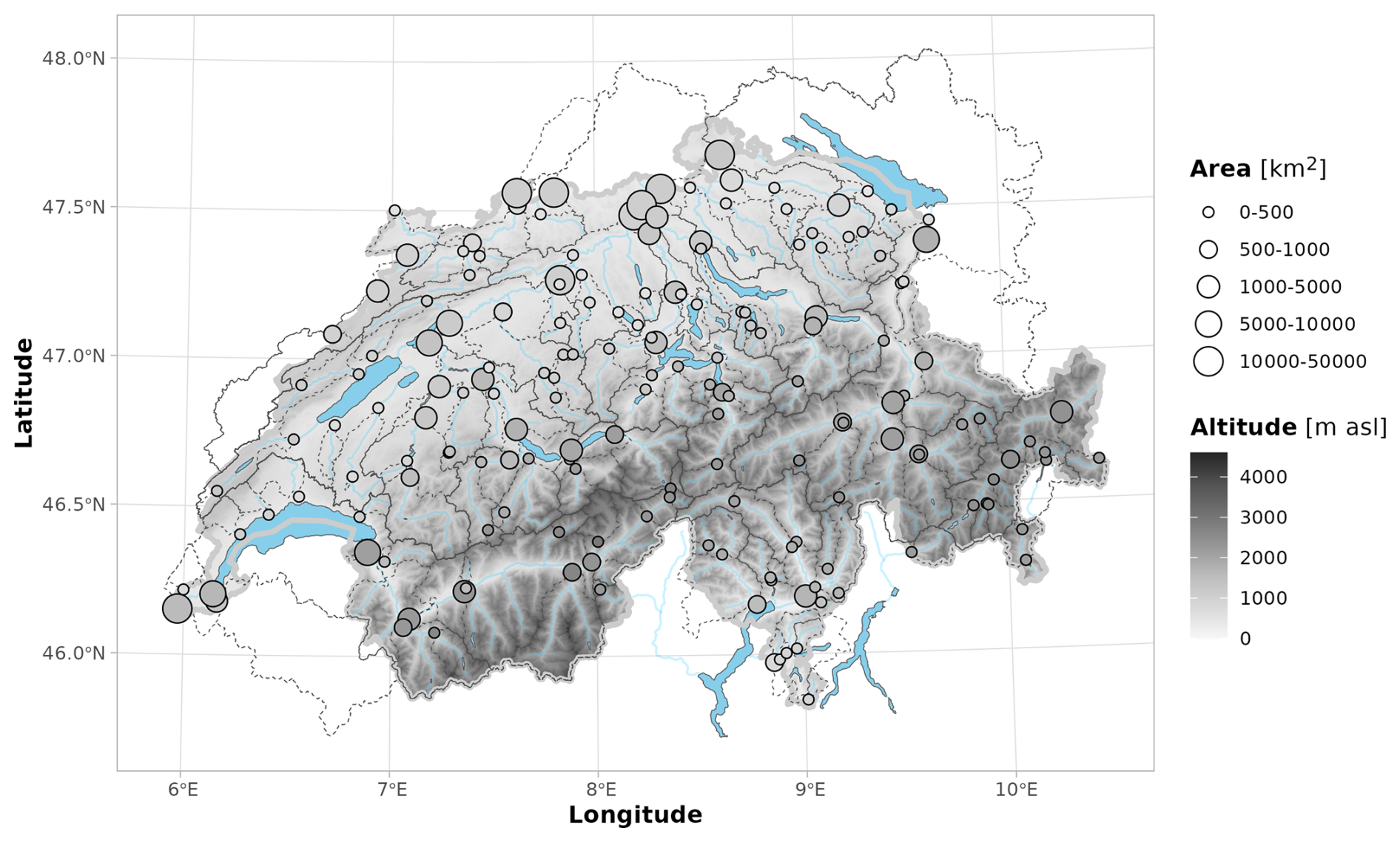
Figure 1 Overview of the study area and catchments included in the HYD-RESPONSES dataset. Catchment outlets (circles) are coloured by mean catchment altitude [m a.s.l.] and the point size scales with the catchment area [km²]. Dashed lines show the catchment outlines. Generalized streamflow networks and lakes are shown in light blue.

Recent studies focused on assessing the benefits of non-standardized (deficit) indices in tracking the drought propagation signal across drought types (see e.g., Brunner and Chartier-Rescan, 2024; Sur et al., 2020; Wu et al., 2020). Non-standardized indices provide physically interpretable and consistent information on deficits which remain inter-comparable across systems (Van Loon, 2015; Raposo et al., 2023; Wu et al., 2020). Examples are the Hydrological Anomaly Index (HAI), the Water Balance Drought Index (WBDI), the cumulative water deficits (CWD), and the potential cumulative water deficit (PCWD) (Stocker et al., 2023; Sur et al., 2020; Wu et al., 2020). Non-standardized indices allow direct quantification of (precipitation) deficits or surpluses associated with the drought propagation into and recovery from a (hydrological) droughts (Wu et al., 2020) and hence provide valuable information for proactive water management and decision-making (Xu et al., 2023; Parry et al., 2018).

Here, we present a novel dataset with high-resolution observational daily catchment-level time series for key hydro-meteorological variables (including precipitation, snow water equivalent, temperature, soil moisture, (potential) evaporation and streamflow), standardized and non-standardized (drought/deficit) indices (SPI, SPEI, SMRI, CWD, PCWD, CQD) and (streamflow) drought events covering 184 small to large catchments in Switzerland. The HYD-RESPONSES dataset can be combined with existing hydro-meteorological time series datasets and catchment descriptors such as CAMELS-CH (Höge et al., 2023a), which provides large-sample hydro-meteorological data for hydrologic Switzerland (i.e., all catchment areas that drain into Switzerland) and is the Swiss version of the “Catchment Attributes and MEteorology for Large-sample Studies” (CAMELS; see e.g., Clerc-Schwarzenbach et al., 2024). The remaining paper is structured as follows: in Sect. 2 the study region and the catchments are presented. Section 3 introduces all datasets used to compile the HYD-RESPONSES dataset. Section 4 elaborates on the processing of hydro-meteorological data. Section 5 is the analogue for the processing and extraction of catchment descriptors. Section 6 finally discusses the dataset and points to potential caveats and cautionary notes while Sect. 7 presents multiple complementary datasets which are valuable in combination with the HYD-RESPONSES dataset. Section 9 provides a concluding summary. Three exemplary use cases to illustrate the nature and potential of the HYD-RESPONSES dataset are provided in Appendix A.

2 Study region and catchments

The 184 catchments (Fig. 1) provided in the HYD-RESPONSES dataset span a wide range of catchment areas (0.56–35 878 km²), glaciation percentages (0 %–56 %), altitude ranges (467–2937 m a.s.l.) and 18 streamflow regime types (see Fig. 2). Roughly two thirds of the catchments 64.7 % (n=119) are small to mid-size with an area of between 10 and 500 km². Only 9 (4 %) catchments are smaller than 10 km² and 56 (30.4 %) catchments are larger than 500 km². The dataset contains eight very large catchments with areas between 10 000 and 50 000 km² (max. area = 35 878 km²), associated with the three largest rivers in Switzerland: Aare, Rhine and Rhone. Most catchments (82.5 %) have less than 5 % glaciated area. In terms of mean catchment height (elevation), the catchments are distributed relatively equally between 500 and 2500 m a.s.l. (see Fig. 2c). Only eight catchments are higher than 2500 m a.s.l. and only one catchment is at very low elevation (catchment Wiese, Basel). Streamflow regime types were classified and adjusted by the FOEN based on data from the Hydrological Atlas of Switzerland Table 5.2 (https://hydrologischeratlas.ch/downloads/01/content/Tafel_52.pdf, last access: 18 May 2026). Catchments smaller than 500 km² are characterized by considering mean altitude and catchment glaciation percentage to reflect the contribution of specific streamflow (drought) generating processes (glacial, nival, pluvial). Catchments larger than 500 km² are generally classified as mixed regime (>500 km²) type and contain catchments characterized by a combination of streamflow (drought) generating processes. For more information see also Aschwanden and Weingartner (1985) and Fig. 2e.

Note that 12.5 % (n=23) of the catchments have at least 5 % of catchment area lying outside of the Swiss national borders as the dataset consists of catchments of the entire hydrological Switzerland (catchments that drain in(to) Switzerland). Furthermore, the Swiss streamflow monitoring network is designed such that multiple measurement stations may be located along the same river. As a result, upstream catchments can be nested within larger downstream catchments, leading to hierarchical dependencies.

3 Input data products

In this section, the input datasets used to produce and compile the HYD-RESPONSES dataset are presented and reference literature for further reading and more detailed information is provided. Original data products are provided by the Federal Office for Climatology and Meteorology (MeteoSwiss), the Federal Office for the Environment (FOEN), the Swiss Federal Office of Topography (Swisstopo), the Federal Office for Agriculture (FOAG), the WSL Institute for Snow and Avalanche Research (SLF) and the European Centre for Medium-Range Weather Forecasts (ECMWF).

3.1 Catchment-level time series data from streamflow observations

Daily average streamflow measurements at the catchment outlet were provided by the FOEN via the Hydrological Service (https://www.hydrodaten.admin.ch, last access: 18 May 2026) for more than 200 stations. The data availability is station-specific and depends on the installation and FOEN-internal data quality checking. The HYD-RESPONSES dataset only provides a subset of 184 catchments and considers only stations for which an analysis of hydrological drought dynamics in response to cumulative water deficits was deemed to be meaningful in correspondence with the FOEN (Caroline Kan; see Fig. 1). These are stations that provide reliable streamflow (Q) time series and are associated with a physical/natural catchment. Stations are therefore excluded if they (i) only provide water-level information (no Q, 3 stations), (ii) are not part of the main streamflow measurement network (e.g., stations from other networks such as the National Surface Water Monitoring Programme (NAWA BAFU, 2023a), 4 stations), (iii) secondary stations (11 stations), (iv) stations with potential return streamflow (= negative Q values, 2 stations), (v) Q measured at derivations (2 stations), (vi) stations without watershed delineation (i.e., subterranean; 1 station) and (vii) uncertainties in time series composition due to displacement and/or temporarily missing Q of contributing stations (4 stations). The complete list of stations included is provided in Tables B6, B7, B8, B9 and B10 in Appendix B.

3.2 Catchment-level time series data derived from spatially gridded products

Hydro-meteorological variables used in this study were compiled from multiple complementary data sources, combining station-based spatial climate analyses, dedicated snow model products, and reanalysis data (Table 1). This multi-source approach allows both comprehensive coverage of relevant variables and comparative analyses between different data products.

Table 1 (Spatially gridded) Data products used for the time series extraction. Full variable names and associated units are provided in Table B1 (glossary) in Appendix B. Note that the variable short names correspond to the layer/product names in the respective dataset.

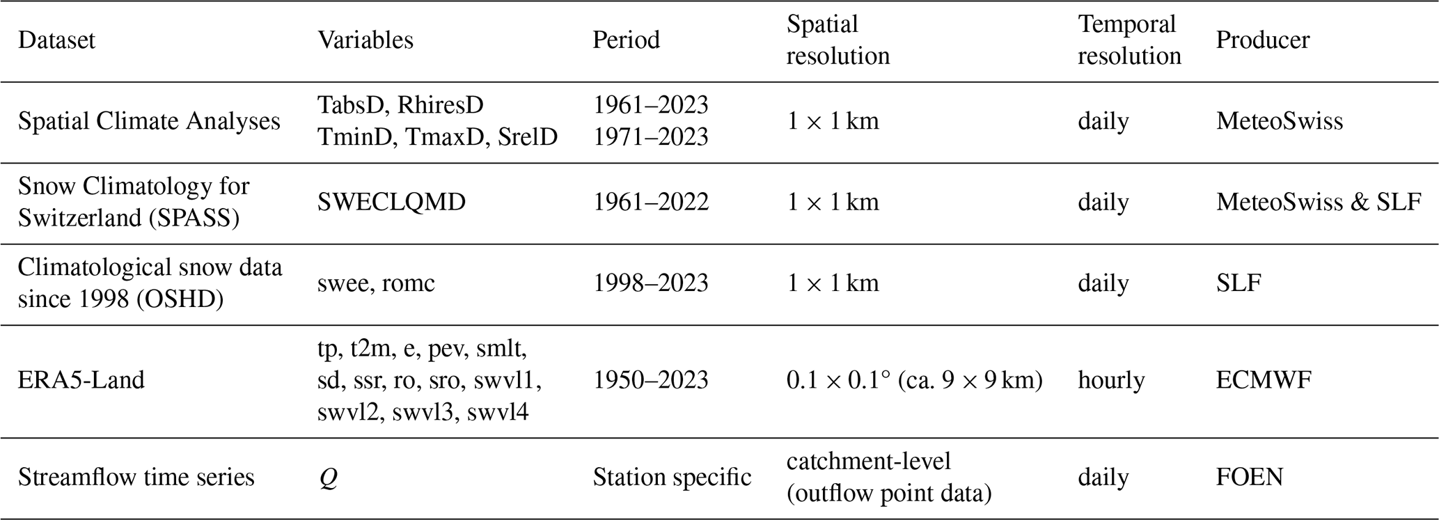
Meteorological variables derived from station-based observations were obtained from the high-resolution (1 × 1 km) spatial climate analyses provided by MeteoSwiss (MeteoSwiss, 2024). These include average 2 m temperature (TabsD), daily minimum and maximum 2 m temperature (TminD, TmaxD), daily precipitation sums (RhiresD), and daily sunshine duration (SrelD) (Frei, 2014; Frei and Schär, 1998; MeteoSwiss, 2021a, b, c). Data availability is product-specific and covers the period 1961–2023 for RhiresD and TabsD and 1971–2023 for TminD, TmaxD, and SrelD. The spatial climate analyses generally cover the Swiss territory only, with the exception of RhiresD, which also includes catchments outside Switzerland that drain through Swiss territory. Note that RhiresD is not available for catchments covering regions in France and Italy before 1992 due to limited meteorological station availability and reduced data reliability (MeteoSwiss, 2021a). Catchments with substantial areas in these regions should therefore be treated with caution or excluded from analyses prior to 1992 (see Sect. 6.2).

Snow water equivalent (SWE) data were compiled from two independent high-resolution (1 × 1 km) snow datasets. The primary source is the spatial Snow Climatology for Switzerland (SPASS) developed jointly by MeteoSwiss and SLF (Michel et al., 2024; Marty et al., 2025). This dataset provides modelled and bias-corrected daily SWE for September 1961–September 2022, derived using the SnowQM model based on TabsD and RhiresD. The SnowQM model is presented in detail in Michel et al. (2024). The spatial coverage is restricted to Switzerland. A second snow dataset is derived from the Swiss Operational Snow-Hydrological model system (OSHD), provided by WSL (SLF), which supplies SWE and modelled snowmelt runoff for the period 1998–2022 (Mott, 2023; Mott et al., 2023).

All remaining hydro-meteorological variables, including evaporation, potential evaporation, soil moisture, and additional variables overlapping with the datasets described above, were extracted from the ERA5-Land reanalysis provided by ECMWF (Muñoz-Sabater et al., 2021). Several variables are thus available from multiple sources and are retained in the HYD-RESPONSES dataset to enable inter-product comparisons. Variables covered by more than one data source include air temperature (TabsD, TminD and TmaxD from MeteoSwiss, t2m from ERA5-Land), precipitation (RhiresD from MeteoSwiss, precipitation from ERA5-Land), snow water equivalent (SWE; from SPASS, OSHD, and ERA5-Land) and modelled snowmelt (from OSHD and ERA5-Land). Additional ERA5-Land-specific variables include soil water volume (swvl) at four depths, total solar radiation (ssr), total runoff (ro), and surface runoff (sro). Detailed variable descriptions are provided in the dataset documentation on Zenodo (von Matt et al., 2026). A glossary for the variable abbreviations is provided in Table B1.

ERA5-Land data are available at hourly resolution for the period 1950–2023 via the Copernicus Climate Data Store (CDS) (https://cds.climate.copernicus.eu/datasets/reanalysis-era5-land, last access: 18 May 2026). ERA5-Land consists of numerical model output from the ECMWF land surface model which itself is driven by downscaled and elevation-corrected meteorological forcing from ERA5 (Muñoz-Sabater et al., 2021). The higher spatial resolution (0.1 × 0.1°, approximately 9 × 9 km) results in an enhanced soil moisture representation and river discharge estimations making ERA5-Land more suitable for analyses based on the hydrological cycle than ERA5 (Muñoz-Sabater et al., 2021).

The procedures used to extract time series from all gridded datasets are detailed in Sect. 4.

3.3 Catchment-level time-invariant data (catchment descriptors)

Datasets used to compile an extensive set of catchment descriptors include station metadata and information on time series availability and homogeneity provided by the FOEN as well as spatial (polygon) data on hydro-terrestrial characteristics (e.g., soil characteristics, hydro-geology) provided by the FOEN, FOAG and Swisstopo (see Table 2). Most information is available from https://www.opendata.swiss (last access: 18 May 2026), the FOEN Hydro-Service (https://www.hydrodaten.admin.ch (last access: 18 May 2026), or can be downloaded and inspected via https://www.map.geo.admin.ch (last access: 18 May 2026) (Swisstopo). Direct links to the datasets are provided below and in Sect. 8, Code and data availabilty.

Table 2 Data products used to extract catchment descriptors.

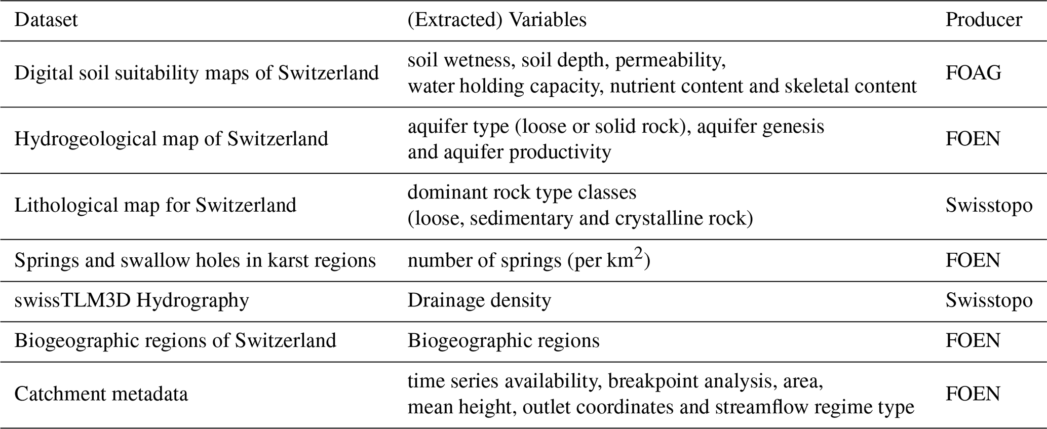
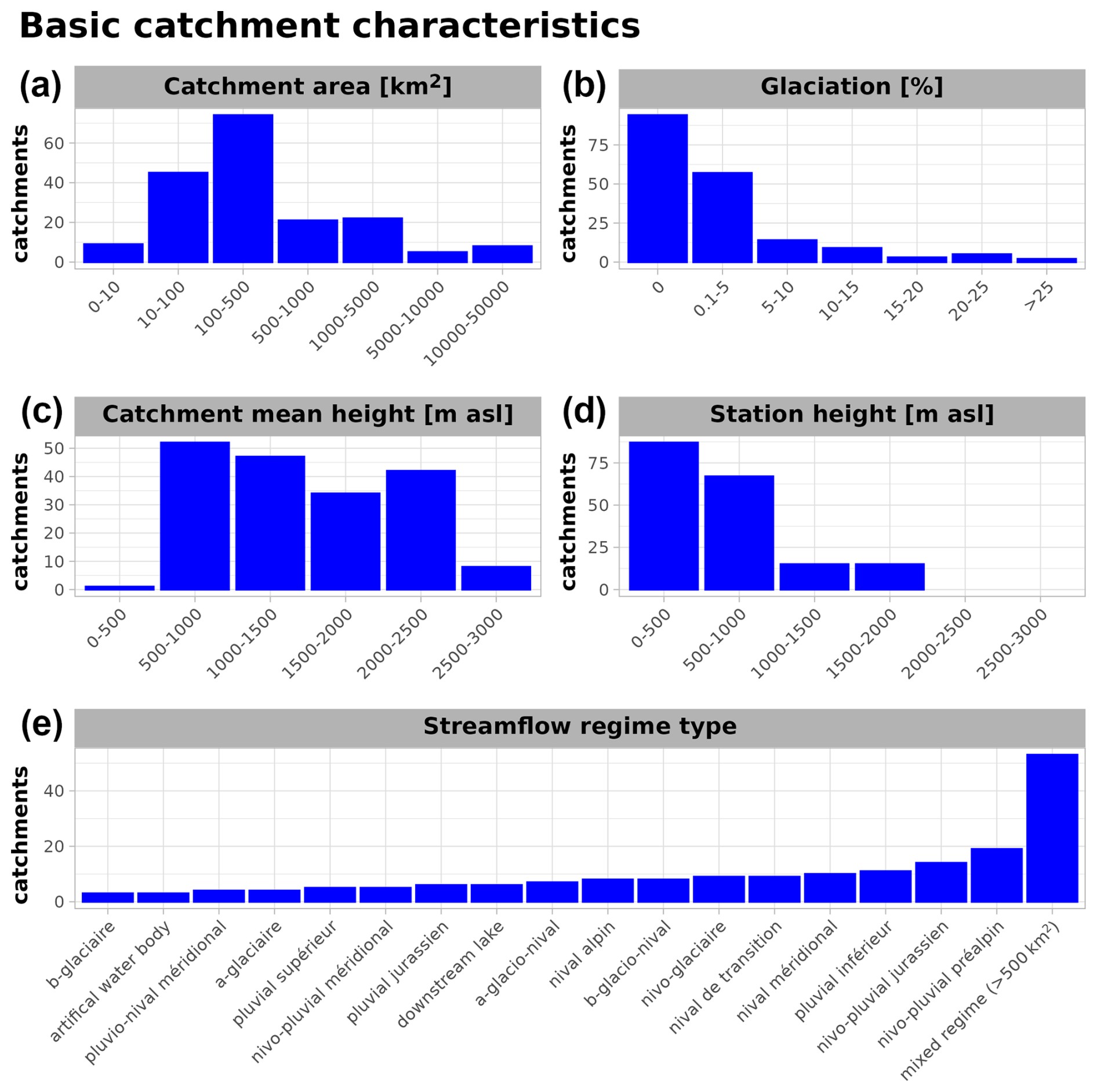
Figure 2 General catchment characteristics provided by the FOEN. (a) Catchment area in km², (b) Glaciation percentage (of catchment area), (c) catchment mean height [m a.s.l.], (d) height of the streamflow gauge measurement station [m a.s.l.] and (e) streamflow regime types. The y-axis shows the number of catchments in each category.

The digital soil suitability maps of Switzerland provide information on a set of different soil characteristics assessed on 25 different geological and geomorphological units which are further discriminated by different landscape elements depending on aspect, slope and bedrock. The maps were first assessed in 1980 and revised in 2000 (BLW, 2022; Swisstopo, 2020). The different soil characteristics include soil wetness (https://opendata.swiss/de/dataset/digitale-bodeneignungskarte-der-schweiz-vernassung, last access: 18 May 2026), soil depth (https://opendata.swiss/de/dataset/digitale-bodeneignungskarte-der-schweiz-grundigkeit, last access: 18 May 2026), permeability (https://opendata.swiss/de/dataset/digitale-bodeneignungskarte-der-schweiz- wasserdurchlassigkeit, last access: 18 May 2026), water storage capacity (https://opendata.swiss/de/dataset/ digitale-bodeneignungskarte-der-schweiz-wasserspeichervermogen, last access: 18 May 2026), nutrient content (https://opendata.swiss/de/dataset/digitale-bodeneignungskarte-der-schweiz-nahrstoffspeichervermogen, last access: 18 May 2026) and skeletal content (https://opendata.swiss/de/dataset/digitale-bodeneignungskarte-der-schweiz-skelettgehalt, last access: 18 May 2026).

The hydro-geological map of Switzerland provides information on groundwater resources in Switzerland (Schürch et al., 2007), including information on aquifer type (loose or solid rock), aquifer genesis and aquifer productivity. The map was originally produced and published for the Hydrological Atlas of Switzerland (HADES, https://hydrologischeratlas.ch/, last access: 18 May 2026). The hydro-geological information was further complemented with the lithological map for Switzerland (produced by Swisstopo), which provides a general overview of dominant rock type classes (loose, sedimentary and crystalline rock). The maps are available via opendata.swiss (https://opendata.swiss/en, last access: 18 May 2026) (hydrogeological map, https://opendata.swiss/de/dataset/hydrogeologische-karte-der-schweiz-grundwasservorkommen-1-500000, last access: 18 May 2026; lithological map https://opendata.swiss/de/dataset/lithologisch-petrografische-karte-der-schweiz-gesteinklassierung-1-500000, last access: 18 May 2026) or can also be accessed via the Hydrological Service of the FOEN (https://www.bafu.admin.ch/bafu/de/home/themen/wasser/zustand/karten/geodaten.html, last access: 18 May 2026). The number of springs and swallow holes in karstic regions provides additional information related to aquifers and the contribution of subsurface water storage. The layer provides main discharge source locations in karstic regions and is available via opendata.swiss (https://opendata.swiss/de/dataset/quellen-und-schwinden-in-karstgebieten, last access: 18 May 2026) (produced by FOEN). The swissTLM3D Hydrography provides topological information on the different water bodies of Switzerland (including flowing and stagnant waters) and originates from the swissTLM3D dataset provided by and accessible via Swisstopo (https://www.swisstopo.admin.ch/de/landschaftsmodell-swisstlm3d#swissTLM3D---Download, last access: 18 May 2026).

The biogeographic regions of Switzerland provide six regions differentiated by similarity of flora, fauna, bryophytes and ornithological information as well as homogeneous surface water catchments (BAFU, 2022). Biogeographic (eco-)regions often correspond well to catchment groups with similar streamflow regime types and are therefore frequently used for catchment regionalization (e.g., Jehn et al., 2020; Guo et al., 2021). The biogeographic regions are available via opendata.swiss (https://opendata.swiss/de/dataset/biogeographische-regionen-der-schweiz-ch, last access: 18 May 2026).

Finally, general information on the gauging stations and streamflow time series (availability and homogeneity) were provided as accompanying (meta-)data by the FOEN. Time series homogeneity was derived by the FOEN using breakpoint tests following the method of Bai and Perron (1998). Breakpoints are identified by partitioning the time series based on the number of potential breakpoints and subsequent modeling of the time series by piecewise linear regression (see Bai and Perron, 1998). The optimal breakpoints are found by minimization of the sum of squared residuals. Resulting breakpoints are indicative to changes in the mean annual 7 d mean flow (M7Q) and were further plausibilized by the FOEN based on catchment meta information and known (potentially) relevant anthropogenic influences such as the construction of (reservoir) dams, hydropower and wastewater treatment plants (for more information see BAFU, 2024). General station information includes catchment area, mean catchment height (elevation), glaciation percentage, outlet coordinates and streamflow regime type (among others) (see Figs. 1 and 2). Catchment outlines (polygons provided by the FOEN) and catchment outlets (point shapes) are provided in the coordinate system CH1903/LV03 (EPSG:21781).

Note that the digital soil suitability maps, swissTLM3D hydrography, biogeographic regions of Switzerland as well as information on springs and swallow holes in karst regions are restricted to Swiss national territory. Catchments with a significant area outside of Switzerland should be treated with caution regarding descriptive variables extracted from these datasets (see Sect. 5 for a comprehensive overview on extracted descriptors). The hydrogeological and lithological maps of Switzerland to a large extent also cover areas outside of Switzerland. Only catchments of the Rhine (catchments 2091, 2143, 2288, 2289) and Wiese (catchment 2199) are not entirely covered. However, with a coverage of at least > 94 %, descriptors extracted from these datasets may still prove valuable for these catchments.

Methodological details on the extraction and preparation of catchment descriptors are presented in Sect. 5.

4 Processing of hydro-meteorological data

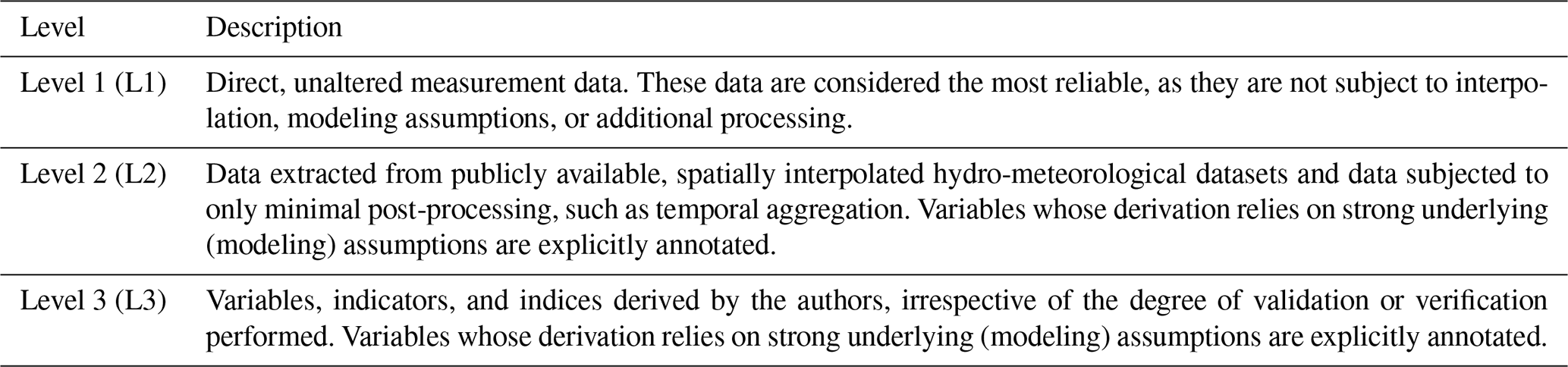
This section describes the methodology used for aggregating spatially gridded (time series) data product, the methods used to derive additional indicators, standardized drought indices, and presents the definition and declaration of (hydrological) drought events. Guidance on the reliability of indicators is provided through a three-level classification based on the origin of the underlying data, the extent to which variables rely on (model) assumptions, and the degree of processing applied to derive the hydro-meteorological data, (drought) indices, and events. Level 1 consists of direct, unaltered measurement data and is therefore considered the most reliable. Level 2 includes data directly extracted from publicly available spatially interpolated hydro-meterological datasets and data subjected to only minimal (post-)processing (e.g., temporal aggregation). Level 3 comprises all variables, indicators, and indices derived by the authors, irrespective of the degree of validation or verification performed. For both Level 2 and Level 3 data, additional annotations are provided for variables whose derivation is based on a (strong) modeling component. A summary of the classification is provided in Table 3.

The naming of the unaltered variables directly retrieved from measurement data (streamflow) or extracted from spatially interpolated hydro-meteorological datasets is based on the layer names used in the original input datasets (see variables listed in Table 1 and the glossary provided in Table B1). Derived variables and (standardized) drought indices are named by a suffix representing the type of indicator followed by all contributing variables where ERA5-Land variables are kept in lowercase while variables from other products start with upper-case letters. Naming for derived variables based on the snow products make use of the product name (SPASS) or the combination of product and variable names (OSHD) as identifier for clear distinction. All extracted and derived variables and their suggested reliability level are listed in the Tables B2, B3, B4 and B5 in Appendix B.

Time series of all categories are illustrated in Fig. 6 showing the exceptional drought year 2022 for the example catchment 2034 – Broye, (Payerne, Caserne d'aviation) located in the western Swiss Plateau region (see catchment contours in Fig. A4). A detailed analysis of the event year 2022 demonstrating the utility of the time series provided in the HYD-RESPONSES dataset is provided in Sect. A2 in Appendix A.

Table 3 Three-level processing classification used for hydro-meteorological data in the HYD-RESPONSES dataset. Note that these classes differ from the satellite data classification.

4.1 Time series extraction

Based on the spatially gridded hydro-meteorological input products (see Sect. 3.2), catchment-level time series were extracted using the R-packages terra (Hijmans, 2023) and exactextractr (Baston, 2023). First, the hourly ERA5-Land data was aggregated to daily resolution following the standards used by the MeteoSwiss spatial climate analyses (e.g., RhiresD and TabsD). For this, instantaneous variables and variables representing accumulations or fluxes are distinguished. For instantaneous variables, we provide daily average values. For variables representing accumulations and fluxes, we provide daily sums. Flux variables (mainly precipitation and evapotranspiration) are aggregated using the same temporal convention as the RhiresD precipitation sums, i.e., from 06:00 UTC (day) to 06:00 UTC (day + 1) (see MeteoSwiss, 2021a). Instantaneous variables and ERA5-Land temperature were averaged from 00:00 to 00:00 UTC again following the convention used in equivalent MeteoSwiss products (e.g., TabsD; MeteoSwiss, 2021b). Daily catchment-average time series were then extracted by using the catchment outlines (polygons) provided by the FOEN. Units were homogenized across time series. Both units and full standard variable names are listed in Table B1 (glossary).

The length of the time series depends on the dataset that they were derived from (see Table 1 for details). Streamflow time series are provided for three different catchment-specific time periods: (1) the original time series (entire period), (2) the time series of the most recent gap-free time-period and (3) the most recent homogeneous time series (in case of significant and plausible breakpoints; otherwise equal to the gap-free time series) (see Fig. 3). The breakpoint information is provided by FOEN (see Sect. 3.3). Information on the start of the streamflow monitoring by water level sensor is also provided. The streamflow data should only be considered reliable after the initialization of a sensor. In case of no breakpoints the gap-free period is equal to the homogeneous period. The homogeneous period is usually the shortest (e.g., in case of breakpoints or water level sensor initialization; see for example catchment 2349 in Fig. 3). In the case of gaps but no breakpoints, both the homogeneous and the gap-free periods are identical (see, i.e., catchments 2239, 2386 and 2368 in Fig. 3). Indicators and (non-)standardized (drought/deficit) indices derived from the hydro-meteorological time series are available for the longest common period of all contributing variables.

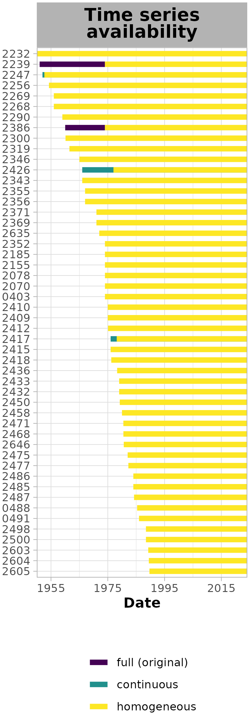
Figure 3 Streamflow time series availability for 50 example catchments. The colours indicate the periods covered by availability type. Full is equivalent to the original time series provided by the FOEN. Continuous denotes the gap-checked time series and the homogeneous period accounts for homogeneity (starting at a breakpoint). In the case of overlapping periods, only the most important period type for analysis (e.g., homogeneous) is displayed. The importance of the periods for analysis is defined as follows: homogeneous is more important than continuous is more important than full (original).

4.2 Derived indicators

4.2.1 Streamflow

Derived indicators related to streamflow consist of the 7 d average streamflow (moving average) M7Q (Fig. 6i). The M7Q (or M7) is often used in low-flow studies and is also used for the official low-flow statistics in Switzerland by the FOEN (see e.g., BAFU, 2024; Muelchi et al., 2021a; von Matt et al., 2024).

4.2.2 Snow related variables

In addition to variables providing direct information on (modelled) snowmelt, also daily differentiated SWE (ΔSWE) time series are provided for both SPASS and OSHD. Snowfall (ΔSWE > 0) and snowmelt (ΔSWE < 0) time series are provided separately. Note that SWE is reset in the SPASS dataset at the end of every snow year (every 1 September) to avoid unrealistically high accumulation of snow water equivalents (“snow towers”; see Michel et al., 2024). As snowfall and snowmelt were derived from daily differences in SWE (ΔSWE), this reset can result in an artificially large negative ΔSWE value on 1 September that does not represent actual physical snowmelt. To prevent this model artifact from affecting the derived snowmelt time series, ΔSWE values on 1 September were set to missing values and replaced by a linear interpolation using the ΔSWE values from the preceding and following days. Snow-corrected precipitation series (P+ΔSWE) were calculated by combining time series of total precipitation (RhiresD and ERA5-Land) and ΔSWE time series (SPASS, OSHD) as well as time series with modelled snowmelt information (SPASS, OSHD and ERA5-Land). Negative snow-corrected precipitation amounts (e.g., RhiresD < ΔSWE) were set to zero.

4.2.3 Water balance

(Potential) Water balance indicators (P–E and P–PET) were derived by combining the total and snow-corrected precipitation time series with the ERA5-Land evaporation and potential evaporation time series.

4.3 Cumulative water deficits

(Potential) Cumulative water deficits (CWD and PCWD) are non-standardized indicators tracking evaporation-driven deficits in the (potential) water balance. CWD and PCWD were derived from the daily water balance indicator time series (see Sect. 4.2.3) using the cwd R-package (Stocker et al., 2023; Stocker, 2021). A deficit starts when the water balance is negative (i.e., $P-E<\mathrm{0}$) and is accumulated as long as the deficit remains uncompensated (deficit > 0). Note that no surplus information is tracked. Once the deficit is compensated, the values remain at zero (CWD =0). Example time series are shown for both CWD and PCWD in Fig. 6k, l. In some cases (especially for P–PET based only on ERA5-Land variables, i.e., tp − pev), PCWDs are not compensated each year and can persist over multiple years. Both CWDs and PCWDs are hence also provided on a yearly calculation basis (annual reset on 31 December). Non-standardized indices preserve units (here millimetres) and are physically interpretable in terms of absolute deficit amounts. Cumulative water deficits do not rely on a predetermined calculation time window, which allows the user to track both deficits accumulated over short periods in time (below one month) and deficits accumulated over very long periods.

Water-balance based non-standardized drought indices are widely in use in ecohydrological, land-atmosphere interaction research and catchment-memory studies both with and without temporal resets (see e.g., Biegel et al., 2025; Cui et al., 2022; Stocker et al., 2023). Being more strongly tied to the actual physical water availability, non-compensated CWDs may provide valuable information on carry-over effects in multi-year drought contexts and/or long-term shifts in climatic water balance (Stocker, 2021; Fowler et al., 2022; Saft et al., 2015). PCWDs in contrast are based on potential water balance and (absolute) carry-over deficits should hence be treated with caution. CWD and PCWD time series which are annually reset provide complementary year-to-year information, which may better align in contexts of annual low-flow statistics and allows for a year-to-year comparison across years and catchments.

4.4 Standardized (drought) indices

Standardized (drought) indices depict the anomaly of a deficit over a fixed retrospective time window (e.g., 1 month). The hydro-meteorological indicator time series is first aggregated over the given window and then transformed to a standard normal distribution by fitting a suitable candidate distribution (Tijdeman et al., 2020; Stagge et al., 2015). Standardized indices therefore provide information on both anomalously dry and wet conditions, which are often defined by thresholds corresponding to standard deviations (SD). As such, values below −1 SD indicate drier than normal conditions (moderate droughts), while values above +1 SD indicate wetter than normal conditions (moderate wetness) (McKee et al., 1993; Tschurr et al., 2020). The HYD-RESPONSES dataset provides daily time series for three standardized (drought) indices: the Standardized Precipitation Index (SPI, McKee et al., 1993), the Snowmelt and Rain Index (SMRI, Staudinger et al., 2014), and the Standardized Precipitation Evaporation Index (SPEI, Vicente-Serrano et al., 2010). The SPI represents deficits driven by precipitation only (derived from P), while the SMRI tracks deficits in liquid water input originating from both rainfall and snowmelt (derived from P+ΔSWE) accounting for seasonal snowfall and snowmelt dynamics (Staudinger et al., 2014; Baez-Villanueva et al., 2024). The SPEI represents deficits driven by evaporative demand (derived from P-PET) and hence indirectly accounts for temperature effects (Vicente-Serrano et al., 2010; Mwinjuma et al., 2026; Gebrechorkos et al., 2025). Daily time series for all three indices (SPI, SPEI, SMRI) are provided for aggregation windows ranging from 1–24 months (31–730 d). Exemplary SPI and SMRI time series for all aggregation windows are shown in Fig. 6g,h.

All indices were calculated using the SCI R-package (Stagge et al., 2015; Gudmundsson and Stagge, 2016) with custom modifications accounting for the daily time series resolution. All candidate distributions provided within the SCI R-package (gamma, genlog, gumbel, lnorm, norm, gev, pe3, weibull) were tested for suitability. The distributions were fitted for each day of the year (DOY) based on the reference period 1991–2020. This results in a fit for each DOY derived from the same (window of) values for each distribution. Monthly SPI fits (SPI-1) are for example based on the 30 daily values up to the specific DOY for each of the 30 years in the reference period 1991–2020. The suitability of candidate distributions was assessed based on three indicators: the Shapiro-Wilks normality tests (p-values; Shapiro and Wilk, 1965), the number of flags returned by the fitting function fitSCI (see SCI R-package;  Gudmundsson and Stagge, 2016), and the number of missing and/or implausible values. Implausible values are defined as values above or below ±3 SD following Stagge et al. (2015). Estimating more extreme standardized index values from a 30-year climatology requires substantial extrapolation of the fitted distribution and is therefore associated with large uncertainty, particularly given the strong temporal autocorrelation of drought indices. Values beyond ±3 correspond to events with return periods far exceeding the length of the reference record and cannot be robustly quantified (see Stagge et al., 2015).

The returned flags in distribution parameter fitting were mainly related to convergence issues (non-convergence) (flag 3, see SCI R-package, Gudmundsson and Stagge, 2016). Without a valid fit, the transformation to standardized index values is not possible resulting in missing values on the flagged DOYs in all time series years. As in Staudinger et al. (2014), one best-fitting distribution (over all DOYs) is chosen for all catchments to allow for catchment comparability. The distribution was selected among the distributions satisfying the following conditions: (1) the transformed values are not significantly different from a normal distribution for the majority of catchments (p-values >0.05 for at least 75 % of the catchments), (2) fewer than 5 DOYs flagged and (3) fewer than 50 implausible and/or missing values in the transformed time series (combined consideration of missing values due to flags and unrealistically high/low values). The distribution selection procedure is illustrated for the SPEI in Fig. 4. The results of the Shapiro-Wilks tests (p-values) and information on missing/implausible values and flags are also provided in the HYD-RESPONSES dataset and can be used to identify catchments with non-satisfying properties within the overall best-fitting distribution (see Fig. 4). Following Stagge et al. (2015), values of all standardized (drought) indices time series were constrained to the interval [−3, 3] SD.

The Gamma distribution was chosen for the SPI for all variables (RhiresD, ERA5-Land), which is consistent with other studies and recommendations of the World Meteorological Organization (WMO) (WMO and GWP, 2016; Stagge et al., 2015; Tschurr et al., 2020; von Matt et al., 2024). The SMRI was fitted by the genlog (lnorm) distribution for the snow-corrected precipitation series based on SPASS (ERA5-Land and OSHD). For the SPEI, the genlog distribution was found to perform best across time scales (see Fig. 4).

SPI, SPEI and SMRI provide complementary (and standardized) information on hydroclimatic variability and drought-related processes facilitating integrated analyses of drought development and propagation and allowing consistent comparisons across catchments, regions and climates (Mwinjuma et al., 2026; Gebrechorkos et al., 2025; Tijdeman et al., 2022). Standardized indices are frequently employed in drought monitoring and early warning systems (DEWS; Tijdeman et al., 2020; Kchouk et al., 2022), drought propagation analysis or as proxy for various storage processes (Haslinger et al., 2014; Cammalleri et al., 2019; Raposo et al., 2023; Peña-Gallardo et al., 2019; Barker et al., 2016). Example use cases for drought event analysis and catchment response patterns are provided in Appendix A2 and A3.

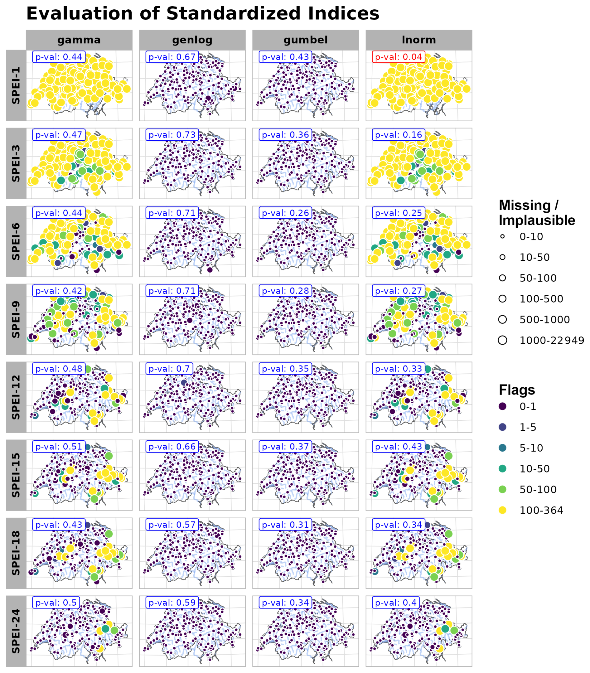
Figure 4 Evaluation statistics for the transformation of standardized (drought) indices. Information on the normality tests (p-values), flags and implausible/missing values (SPEI ∉ [−3, 3]) for four example candidate distributions for the Standardized Precipitation and Evaporation Index (SPEI; Vicente-Serrano et al., 2010). The circle size indicates the number of missing and implausible values Colours show the number of flags (= convergence issues) returned by the fitting function of the SCI R-package (Stagge et al., 2015; Gudmundsson and Stagge, 2016) for all days of the year (DOY). The maximum number of flags is equivalent to 366. Median p-values of the Shapiro-Wilks normality test (Shapiro and Wilk, 1965) were calculated by considering all catchments and are coloured in red in case of rejection (p<0.05). The final HYD-RESPONSES dataset only provides SPEIs fitted by the genlog-distribution (best choice based on the evaluation criteria).

4.5 Climatology & Anomalies

Climatologies and anomalies are provided for all time series, including the time series of variables directly extracted from spatially gridded data products with no modifications except for spatial and temporal aggregation where required (see Sect. 4.1), derived indicators (Sect. 4.2), standardized drought indices (Sect. 4.4), and cumulative water deficits (Sect. 4.3 and 4.6).

Both climatologies and anomalies are based on the reference period 1991–2020. The climatology is provided for two variants: (i) using moving windows and (ii) for fixed time windows. The variants are available at the following time scales: daily (only i), monthly (both), seasonal (both), and annual (only ii). The moving window climatology was calculated by using a moving window of 31 d (day−15, day=0, day+15) for the monthly, a 3-month window (91 d) for the seasonal and a 6-month (183 d) window for the extended season time scale. The moving window climatology is calculated for DOYs 1–366 with NA-values set for 29 February in the case of non-leap years. Example time series for monthly anomalies in 2 m temperature, precipitation, evaporation, soil moisture, snow water equivalent, snowmelt and (potential) cumulative water deficits are shown in Fig.  6a–f, m–n.

The regular climatology is available for monthly, seasonal (DJF, MAM, JJA, SON), extended season (May–October, November–March) and annual time scales. Using the moving window climatology, standardized anomalies have been derived by first subtracting the climatological mean (μ) and then dividing by the climatological standard deviation (σ) (also known as z-scores). The following climatological statistics are provided: minimum, maximum, mean, median, standard deviation, 5th, 25th, 75th and 95th percentiles. For the 7 d average streamflow series (M7Q) we also provide the 2nd, 10th and 15th percentiles which are frequently used in streamflow drought analysis and monitoring (see e.g., Van Loon, 2015; Stahl et al., 2020; Sarailidis et al., 2019; BAFU, 2025).

4.6 Cumulative streamflow deficits

Time series of cumulative streamflow deficits (CQD) were calculated based on negative streamflow anomalies (drought phases) by using the same procedure as for cumulative water deficits (see Sect. 4.3). CQD time series are provided for both fixed and variable threshold definitions. Fixed thresholds (e.g., a constant percentile threshold) are used for critical flow levels that do not change seasonally (e.g., directly linked to physcial/actual low-flow or water scarcity situations) whereas variable thresholds (e.g., seasonally varying percentiles) account for seasonality and changing flow regimes, allowing drought phases and deficits to be identified relative to expected (seasonal) conditions (“anomalies”, Stahl et al., 2020; Van Loon, 2015; Brunner et al., 2019a; von Matt et al., 2024). Hence, variable threshold definitions are often used to analyse seasonally varying streamflow (drought) generating processes or to understand drought propagation mechanisms (Brunner et al., 2023, 2022; Hammond et al., 2022). For the fixed threshold definition, daily M7Q anomalies were derived for events exceeding the Q347 threshold, defined as the daily flow rate exceeded for 347 d yr⁻¹ (i.e., the 347 d exceedance flow, roughly corresponding to the 5th streamflow percentile; see Sect. 5.3). For the variable threshold definition, daily M7Q anomalies were calculated for the following monthly (31 d) and seasonal (91 d) percentiles: 2nd, 5th, 10th, 15th, 25th, 50th (median) and mean. Cumulative deficits are physically interpretable and in the case of cumulative water deficits [mm] and streamflow deficits [m³ s⁻¹] also physically comparable in terms of total runoff depth [mm]. Figure 6j shows CQDs for both fixed and variable threshold definitions for the year 2022 for catchment 2034 – Broye, (Payerne, Caserne d'aviation).

4.7 Identification of drought events

We define drought events as coherent phases of non-zero deficits for cumulative deficits (CWD, PCWD and CQD) and as negative M7Q-based streamflow anomalies for streamflow droughts. Streamflow drought phases were extracted for the same percentiles and time scales as used for CQDs (see Sect. 4.6), namely for monthly (31 d) and seasonal (91 d) percentiles: 2nd, 5th, 10th, 15th, 25th, 50th (median) and the mean. Streamflow events were also extracted for the fixed (yearly) Q347 threshold (see Sect. 4.6 and 5.3).

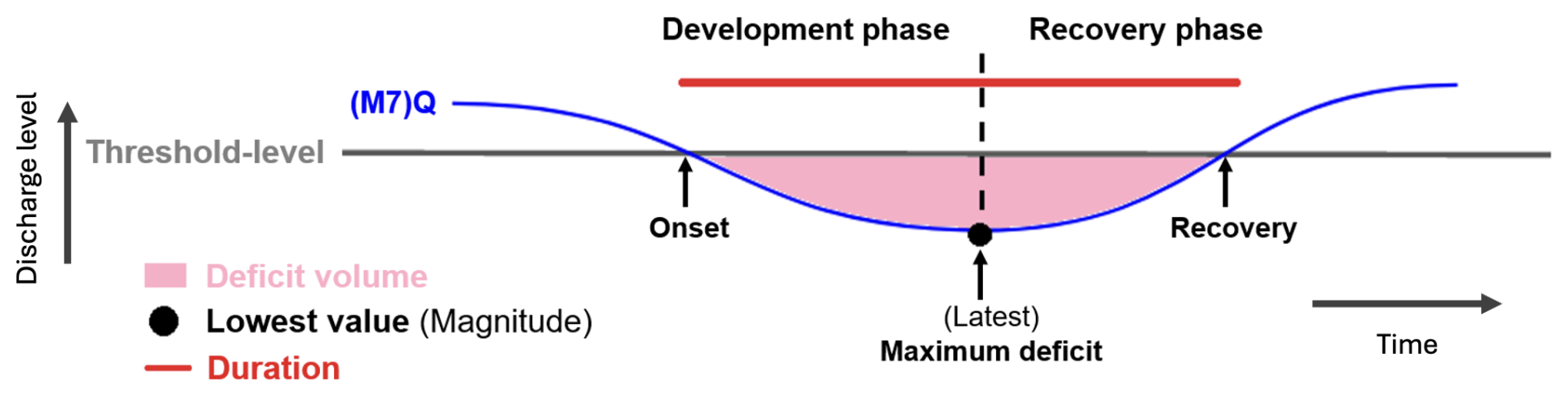
Figure 5 Schematic depiction of the event definition and phase subdivision. The extracted (streamflow) drought phases are characterized by duration, event start (onset), the latest date of the maximum streamflow deficit (anomaly), and event recovery. Additional characteristics are the drought intensity (deficit volume or accumulated deficit) and severity/magnitude (maximum streamflow deficit). The computation of other characteristics is left to the user.

An event starts on the first day values fall below the threshold value and lasts until values exceed the threshold again (see Fig. 5). For each variant, the event time series consists of consecutively numbered event phases and information on the event duration since the start (i.e, an event with a duration of 5 d is represented in the time series as: “1 1 1 1 1” (event phase number), “1 2 3 4 5” (duration since start)). Additional event characteristics (e.g., lowest value during a phase) can easily be derived by the user in combination with the indicator time series. A minor pooling of hydrological drought events is introduced by using the 7 d average streamflow (M7Q) time series which merges closely successing and potentially dependent individual events to one single event as a result of the smoothing of large day-to-day fluctuations (Tallaksen and Van Lanen, 2004; Hisdal and Tallaksen, 2000; Tallaksen et al., 1997; Sarailidis et al., 2019). Streamflow drought events based on both fixed and variable threshold definitions were used for the event shadings in Fig. 6.

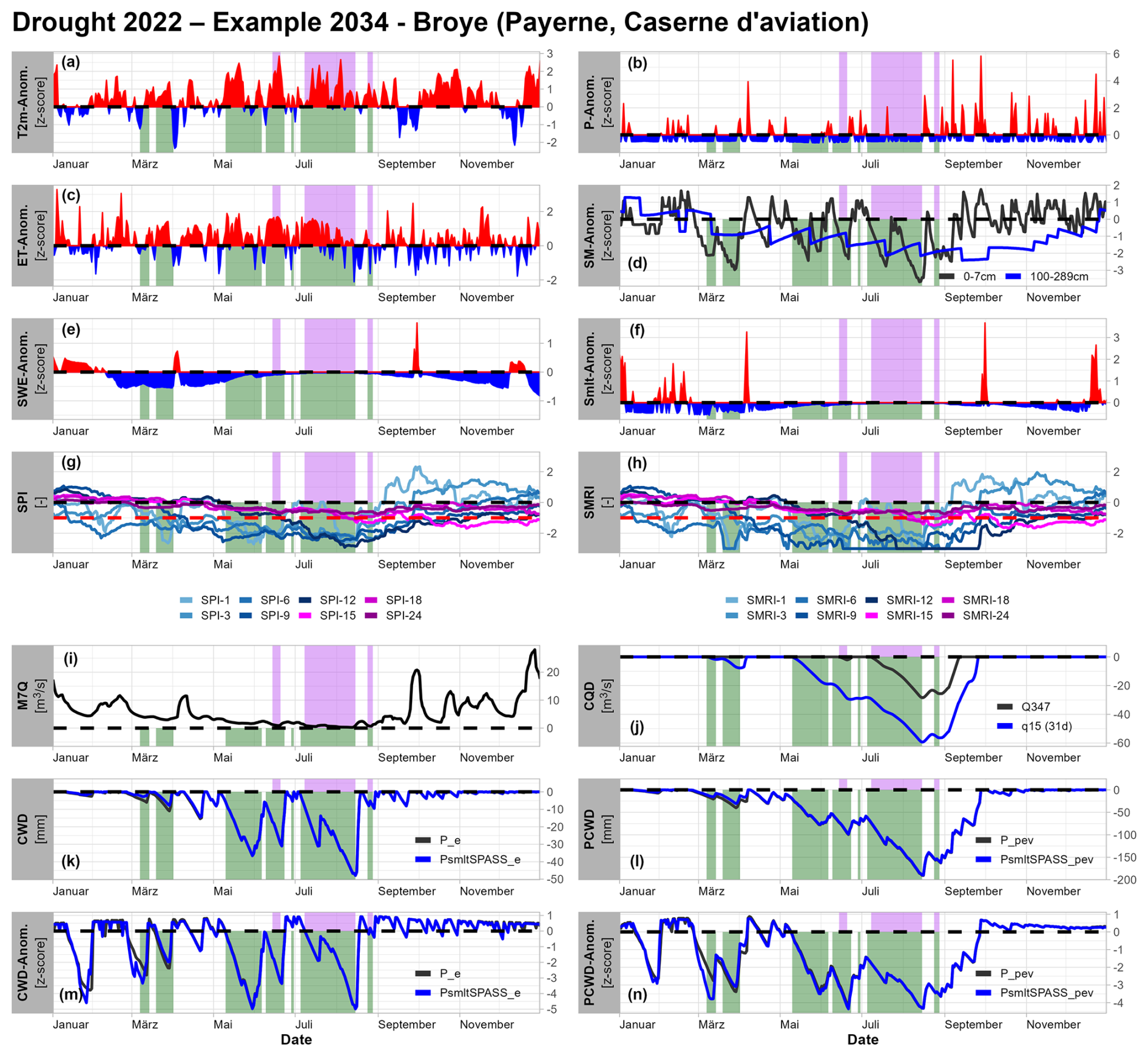
Figure 6 Hydro-meteorological time series for the Swiss Plateau catchment 2034 – Broye, Payerne (Caserne d'aviation) for the year 2022. Color shadings in all panels highlight streamflow drought events for two definitions: yearly Q347 (pink, fixed threshold approach) and a moving monthly 15th percentile threshold (green, variable threshold approach). (a) Moving monthly anomalies of the 2 m-temperature (T2m), positive anomalies are shown in red and negative anomalies in blue. (b) Moving monthly anomalies of the precipitation (P, RhiresD) (c) Moving monthly anomalies of the evaporation (ET, ERA5-land). (d) Moving monthly anomalies of the soil moisture volume (ESM ERA5-land), soil moisture anomalies are depicted for a near-surface SM-level (black, 0–7 cm) and the deepest level (blue, 100–289 cm) available from ERA5-Land. (e) Moving monthly anomalies of the snow water equivalent (SWE SPASS). (f) Moving monthly anomalies of the snowmelt (smlt, SPASS). (g) SPI colored by aggregation scales from 1- to 24-months. (h) SMRI colored by aggregation scales from 1- to 24-months. (i) Seven day average streamflow (M7Q) on which streamflow drought events were identified. (j) The CQD time series shows the corresponding accumulated M7Q-deficits for both the fixed threshold approach (black) and the variable threshold approach (blue). (k) Absolute cumulative water deficit (CWD). (l) Potential cumulative water deficit (PCWD). (m) Monthly anomalies of the CWD (CWD anomaly). (n) Monthly anomalies of the PCWD. Time series of the cumulative water deficits for both absolute values and monthly anomalies are shown for both standard (black, P–E (P_e)) and snowmelt-corrected (blue, P–E+ΔSWE (PsmltSPASS_e)) variants. The same is shown for potential cumulative water deficits which are based on the potential water balance (P–PET (P_pev) and P–PET+ΔSWE (PsmltSPASS_pev)).

5 Catchment descriptors

Catchment descriptors were extracted from spatial datasets containing information on hydro-terrestrial characteristics (e.g., soil suitability maps), catchment (station) metadata (see Sect. 3.3) and the extracted hydro-meteorological time series (e.g., climatology; see Sect. 4.5). All catchment descriptors provide only static (time-invariant) catchment information. Catchment descriptors are provided as single-value catchment-level information. An example use case of catchment grouping/regionalization based on catchment descriptors is presented in AppendixA1.

5.1 Field-based descriptors

Spatially non-overlapping polygon datasets (e.g., soil suitability maps) typically provide categorized values for variable-specific classes (e.g., soil depth classes are shallow, medium, deep, very deep). To extract catchment-level information, polygon-based information was first rasterized to a spatial grid identical to the MeteoSwiss spatial climate analyses grid products (in both extent and resolution). The rasterization was done by using the rasterize function of the terra R-package (Hijmans, 2023). Each grid cell only contains the value of the category with the largest overlap. The percentage overlap with the catchment area was then assessed for all variable-specific classes by using the exact_extract function (as for time series) and adjusting the aggregation function to fractions (“frac”; see Baston, 2023). Catchment area overlap fractions are provided for all categories. Descriptors with multiple classes can also be reduced to a single dominant category represented by the largest percentage overlap (“proportion”). An example is shown for the biogeographic regions in Fig. 7a. Reducing a specific catchment descriptor to one single (dominant) category (e.g., derived via largest overlap percentage) may however lead to a loss in explanatory power as the category with the largest overlap may not necessarily be the most representative or most influential for streamflow (drought) analysis.

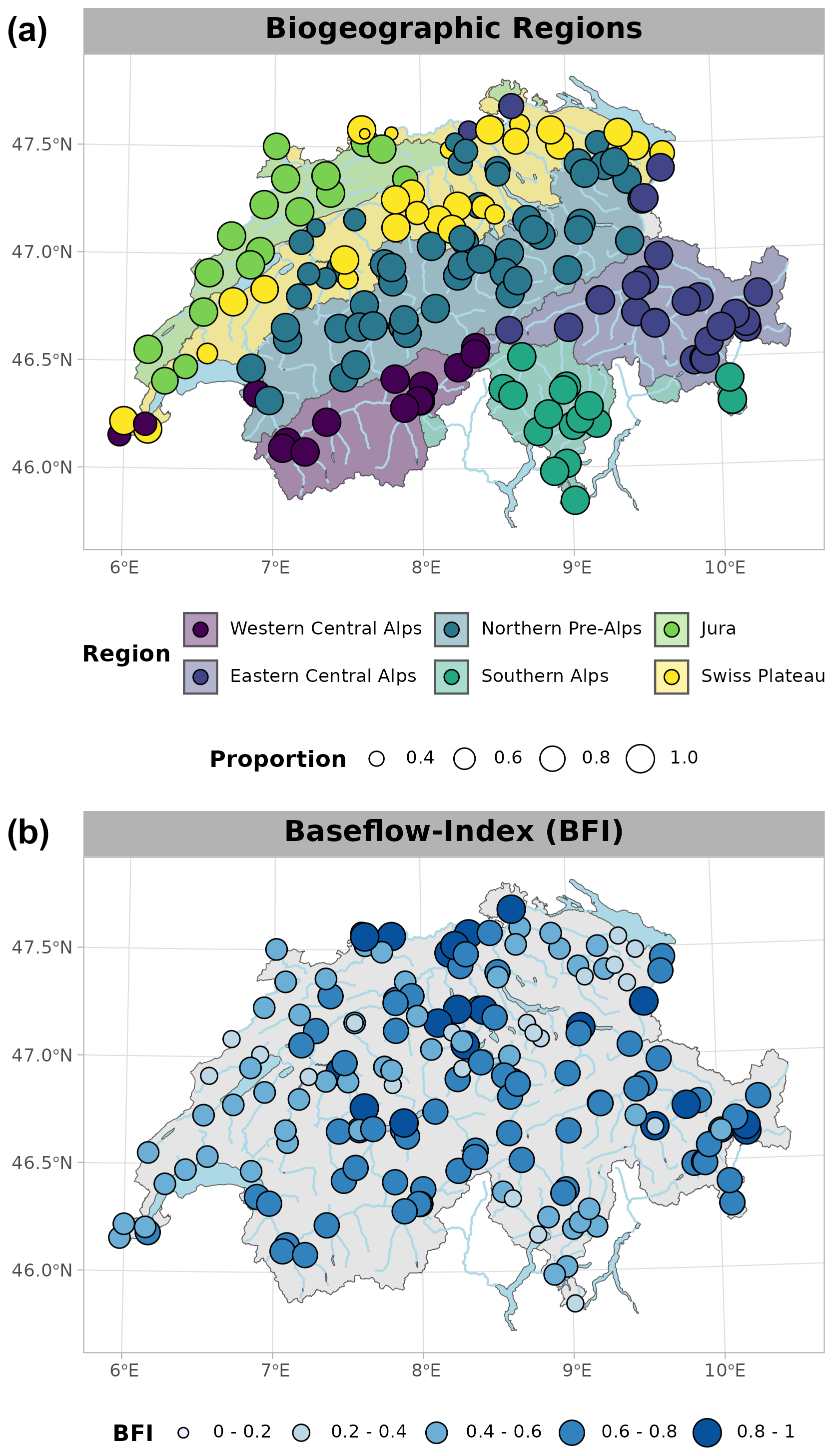
Figure 7 Catchment descriptors (examples). (a) Dominant (largest overlap percentage with the catchment area) biogeographic region (colours). Point sizes indicate the catchment area proportion covered by the dominant biogeographic region. (b) Baseflow-Index (BFI, Nathan and McMahon, 1990) for each catchment derived from the daily streamflow time series.

5.2 Feature-based descriptors

Two descriptive variables related to catchment shape and drainage were derived in R by using the catchment outlines, namely the basin shape index (BSI) and drainage density. The HYD-RESPONSES dataset provides two BSI variants. The first variant is derived based on a ratio between area and basin length ($A/L^{\mathrm{2}}$) known as form factor (Horton, 1932) and the second variant is based on a ratio between the catchment area and the area of the circle with the smallest radius encircling the entire catchment ($A_{\mathrm{catch}}/A_{\mathrm{circle}}$) known as circularity ratio (Miller, 1953). Both indices range from 0 to 1. Both are frequently used (also in combination) as morphometric catchment indicators (see e.g., Das et al., 2022; Pisupati and Ratnakar, 2025). Albeit providing similar information, the form factor is primarily controlled by basin length and hence provides information on catchment elongation, while the circularity ratio is more sensitive to basin shape accounting for complex/irregular shapes resulting in larger areas (for more information on basin shape indices see Das et al., 2022). The drainage density denotes the ratio between the catchment area and the total length of streamflow channels (both natural and stormwater drainage infrastructure; Dingman, 1978; USGS, 2023). The drainage density was calculated by using the swissTLM3D hydrography dataset (see Sect. 8 for a download link). Both indices (BSI and drainage density) are frequently used in flood-related studies but may also provide valuable information during low-flow periods as high-intensity precipitation events are a relevant factor for (streamflow) drought recovery (Eekhout et al., 2018; Floriancic et al., 2022; Lee and Ajami, 2023; Matanó et al., 2024; Qiu et al., 2021; Tarasova et al., 2024; Vicente-Serrano et al., 2022; Wu et al., 2022; Xu et al., 2023). Further, also the overlap percentage with the Swiss territory (swissBOUNDARIES3D, see Sect. 8 for a download link) is provided for each catchment and can be used to exclude catchments with significant portions outside of Switzerland which goes along with a limited coverage in both hydro-meteorological and catchment descriptor input datasets (see Sect. 3.2 and 3.3) for ca. 12.5 % of catchments (see Sect. 2). Information on karstic sources and sinks is provided as the number of sources and swallow holes per catchment and km².

5.3 Time series-based and climatological descriptors

Several indices related to streamflow characteristics (low flow, responsiveness, baseflow and flow stability) are provided in the HYD-RESPONSES dataset. The Q347 (Aschwanden, 1992; Aschwanden and Kan, 1999) is a low flow index used as the basis for water abstraction restrictions in Switzerland and corresponds to the daily flow rate exceeded for 347 d yr⁻¹. The Q347 was derived from the flow duration curve (FDC) by using the hydroTSM R-package (Zambrano-Bigiarini, 2020) and corresponds roughly to the 5th streamflow percentile (95th percentile of 365 d ≈ 347, hence Q347). The baseflow index (BFI; Nathan and McMahon, 1990) is a widely used index linked to multiple catchment characteristics such as aquifer type, productivity and soil characteristics. The BFI provides information on the (base-)flow sustained during dry periods (e.g., by subsurface storages; Tallaksen and Van Lanen, 2004; Bloomfield et al., 2021; Van Loon and Laaha, 2015). The BFI was derived using the baseflow function of the lfstat R-package (Laaha and Koffler, 2022) and is shown in Fig. 7. Stoelzle et al. (2020) introduced the delayed-flow index (DFI) which breaks down the BFI into individual hydrograph components. The components include fast, intermediate, slow and base responses and potentially reflect various storage processes contributing to the overall streamflow response (e.g., snowmelt and groundwater). The DFI was derived by using the delayedflow R-package (https://modche.github.io/delayedflow/, last access: 18 May 2026; see also Stoelzle et al., 2020). The last two indices related to streamflow behaviour are the “flashiness” or R-B-index (Baker et al., 2004) which represents the ratio of the sum of day-to-day streamflow changes divided by the total streamflow and the flow-stability index which relates the mean annual minimum flows (MAM_q) to the mean annual flow (MQ; MAM${}_q/$MQ). The remaining catchment descriptors were derived from the extracted hydro-meteorological time series and/or their respective climatology. Information on average precipitation, temperature, evaporation, snow water equivalent, streamflow, the fraction of precipitation falling as snow and the runoff fraction ($Q/P$) are provided on yearly scales for identifying broad climatic (i.e., water balance) and physiographic controls on hydrological behavior. Finally, monthly Pardé coefficients (PCs) are provided which indicate the contribution of monthly mean streamflow to the annual mean streamflow.

6 Discussion

6.1 Relevance and Applications

The HYD-RESPONSES dataset addresses fundamental challenges in hydrological drought analyses by compiling and harmonizing multiple data sources into a coherent catchment-scale framework, enabling multi-variable drought analyses in Switzerland. Drought (deficit) indices derived from two high-resolution snow climatologies for Switzerland (SPASS, OSHD) also allow for in-depth quantitative analyses on the contribution of snow processes to cross-seasonal drought propagation in Alpine catchments (Staudinger et al., 2014, 2017; Brunner et al., 2023). A combined used of standardized indices (SPI, SPEI, SMRI at 1–24 month scales) and non-standardized cumulative deficits (CWD, PCWD, CQD) facilitate multi-scale (drought) deficit and catchment response sensitivity assessments and allows for a concurrent anomaly-based and physically interpretable characterization of drought deficits (Raposo et al., 2023; Van Loon, 2015; Wu et al., 2020; Baez-Villanueva et al., 2024; Stocker et al., 2023). By providing time series for many relevant variables for drought monitoring (precipiation, temperature, evaporation, soil moisture and streamflow; see e.g., WMO and GWP, 2016) at daily temporal resolution, the HYD-RESPONSES dataset may also be used for training machine learning models such as Random Forests (RFs; e.g., Floriancic et al., 2022) or Long Short-Term Memory models (LSTMs; see Kratzert et al., 2018; Lees et al., 2022; Kratzert et al., 2023) which have recently emerged as promising approach for rainfall-runoff modeling (Kratzert et al., 2018, 2019; Lees et al., 2022). Three example applications of the HYD-RESPONSES dataset are illustrated in Appendix A1, A2 and A3.

Although the dataset was developed for Switzerland, the methodological framework – combining in-situ observations, gridded products, and reanalysis into catchment-scale time series – is transferable, with requirements that scale with data availability. Replication requires four essential components: (1) streamflow observations with defined catchment boundaries, (2) meteorological forcing data (precipitation, temperature), (3) snow information for mountain regions, and (4) static catchment descriptors (e.g., information on soils, geology, topography). While the first component is often limiting, the second component is decisive for the applicability of the dataset on specific use cases. Switzerland can leverage from high-density observational station networks resulting in high-quality spatially gridded hydro-meteorological products (see e.g., MeteoSwiss, 2024). With known biases in mind (especially over complex terrain), ERA5-Land is a viable alternative by providing temporally and physically consistent variables at sufficiently high spatial resolution for comparative catchment studies and machine learning applications aiming for generalizable results in regions where observational networks are less dense (Muñoz-Sabater et al., 2021; Dalla Torre et al., 2024; Scherrer et al., 2023). For local operational drought management or absolute deficit quantification, reliable high-resolution observational products remain however preferable. Several recent developments address observational data limitations, including the Caravan global community dataset (Kratzert et al., 2023), rapidly advancing machine learning-based bias correction methods for downscaling reanalysis products such as ERA5-Land (Menapace et al., 2025; Najafi et al., 2026; Zhang et al., 2025) or advances in developing high-quality remote sensing-based products for soil moisture (e.g. SMAP; see Brocca et al., 2024b; An et al., 2025), snow (e.g., ICESat-2 Besso et al., 2024), evaporation (see e.g., Anderson et al., 2024) and terrestrial water storage (e.g., GRACE-FO; Rodell and Reager, 2023).

6.2 Limitations and cautionary notes

The HYD-RESPONSES time series are provided for product-specific periods, and the spatial coverage is restricted to Swiss territory for most of the higher resolution MeteoSwiss and SLF products (TabsD, TminD, TmaxD, SPASS, SrelD, OSHD) as well as many catchment descriptor input datasets. Full coverage over the entire hydrological Switzerland is only available for ERA5-Land (all variables) and the MeteoSwiss RhiresD product (after 1992; see MeteoSwiss, 2021a). Catchments with significant areas outside of the Swiss national borders – approximately 12.5 % of the catchments (see Sect. 2) – may therefore be considered with caution or used solely for time series based on ERA5-Land variables only. Time series for standardized drought indices are provided only for the transformation variant based on the best-fitting distribution across all catchments to allow for comparison across catchments comparability (see e.g., Staudinger et al., 2014). The best-fitting distribution may however vary across catchments and climates (see e.g., Stagge et al., 2015). The HYD-RESPONSES dataset therefore also provides information on fits, missing values, and flags which can be used to exclude catchments with unsatisfying fitting and transformation properties from analyses. Field- and feature-based catchment descriptors were aggregated at catchment level via summarization (e.g., karstic sources) or percentage overlaps (see Sect. 5.1). Maximum percentage overlaps with catchment area may however only insufficiently account for spatial differentiation which could enhance the representation of factors most influential to streamflow evolution by accounting for spatial proximity to the stream/river courses (Tarasova et al., 2024; Floriancic et al., 2022).

Several known limitations are further related to the datasets used to compile the HYD-RESPONSES data. ERA5-Land is a state-of-the-art reanalysis product provided at a higher spatial resolution than the standard ERA5 reanalysis (Hersbach et al., 2020; Muñoz-Sabater et al., 2021). The higher spatial resolution results in a better depiction of soil moisture, lakes, river discharge estimations, and the orographic enhancement of precipitation (Muñoz-Sabater et al., 2021). ERA5 and ERA5-Land datasets however share most of the parameterizations, as ERA5-Land consists of output from the ECMWF land surface model driven by downscaled and elevation-corrected ERA5 data (Muñoz-Sabater et al., 2021). Despite the advantage of higher spatial resolution over ERA5, a grid resolution of 9 km still has limitations over complex high-altitude terrain. The extracted time series related to snow water equivalent should be used with caution, as snow depth in ERA5-Land is of mixed quality depending on geographical location and altitude (Dalla Torre et al., 2024). Scherrer et al. (2023) showed that ERA5-Land overestimates SWE at high elevations with larger biases in the southern compared to the northern Alps. Higher-resolution datasets such as SPASS (Marty et al., 2025) and OSHD (Mott, 2023; Mott et al., 2023) should hence be preferred over ERA5-Land. Note however that all snow-related datasets have problems in representing small SWE amounts at low altitudes (Scherrer et al., 2023; Michel et al., 2024; Marty et al., 2025). Caution is also required when using the snow-corrected precipitation (water input) time series. The time series corrected by the ΔSWE series consider both snowfall (ΔSWE > 0) and snowmelt (ΔSWE < 0), while the correction based on snowmelt variables only accounts for snowmelt (smlt in ERA5-Land and romc in OSHD; see Tables 1, B1, B2 and Sect. 4.2.2). Snowmelt-corrected precipitation time series may therefore be of limited use during the main snow accumulation season but can still provide valuable information during the snowmelt season.

Another limitation of the ERA5-Land dataset is the parameterization of subgrid-scale processes and the representation of subsurface storages that affect evapotranspiration (e.g., fixed maximum storage volume assumption; see Muñoz-Sabater et al., 2021). Key processes such as dynamic groundwater–vegetation interactions, irrigation withdrawals, and adaptive rooting strategies are hence not represented and may lead to biases in evapotranspiration responses (Muñoz-Sabater et al., 2021; Dalla Torre et al., 2024; Wood et al., 2025; Stocker et al., 2023). Although ERA5-Land compares more favorably with in situ soil moisture and evapotranspiration observations than previous reanalyses (e.g., ERA5), considerable discrepancies remain, especially in dry summers and in regions with heterogeneous land cover (Scherrer et al., 2022; Fluhrer et al., 2025). Given these limitations, drought indicators based on ERA5-Land evapotranspiration should generally be interpreted with caution. This limitation is further compounded by the fact that the validation of long-term soil moisture and evapotranspiration remains challenging due to the scarcity of consistent observational datasets, particularly at high spatial resolution and over multi-decadal time scales (Hirschi et al., 2020; Yi et al., 2024; Mukherjee et al., 2018). Many state-of-the-art evapotranspiration products are limited in temporal or spatial extent and can be affected by gaps and cloud contamination (e.g., remote sensing-based products; see Yi et al., 2024). ERA5-Land thus remains one of the few datasets providing spatially consistent and continuous long-term evapotranspiration estimates with sufficiently high spatial resolution over Switzerland.

Additional caution is warranted when using HYD-RESPONSES water balance time series (and indicators derived from them) when they were derived by combining ERA5-Land evapotranspiration with (snow-corrected) precipitation from independent data sources (RhiresD, OSHD, and SPASS). While ERA5-Land variables are internally consistent, the combination with independent data sources may lead to systematic biases in absolute deficit estimates. This limits the interpretability of absolute cumulative deficits but does not invalidate the approach for comparative, process-oriented drought analyses across regions and catchments (e.g., drought propagation, catchment response sensitivities). Relative measures of cumulative deficits, their temporal evolution, and their normalization through ratios (e.g., CWD/PCWD) can still provide valuable insights, even when absolute magnitudes are uncertain. In such contexts, relative anomalies, temporal evolution, and spatial patterns are more informative than absolute deficit magnitudes. Studies have further demonstrated coherent representation of major drought events (e.g., drought years 2003 and 2018) across datasets, which supports the usability of combined indicator time series when known limitations are adequately taken into account (Scherrer et al., 2022; Wood et al., 2025). Note that the HYD-RESPONSES dataset also provides complementary water balance and SPEI time series derived from ERA5-Land variables only, providing consistent metrics and opportunity for comparisons among data products. Guidance on the usage and reliability of all HYD-RESPONSES time series products is provided by a classification based on three reliability levels (see Sect. 4 and Table 3). The levels are based on the origin of the underlying data, the extent to which variables rely on (model) assumptions, and the degree of processing applied to derive the hydro-meteorological time series.

7 Complementary datasets

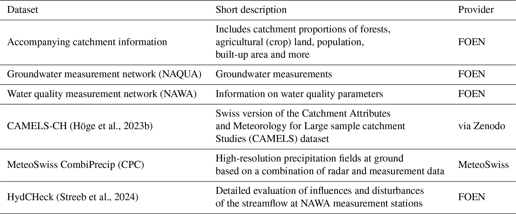
Complementary datasets provide a wide range of additional catchment descriptors and hydro-meteorological time series. An overview of datasets and variables is provided in Table 4. The FOEN provides additional geodata related to both surface and groundwater via the Hydrological Service (https://www.bafu.admin.ch/bafu/de/home/themen/wasser/zustand/karten/geodaten.html, last access: 18 May 2026). The datasets include additional catchment descriptors with information on population density, catchment areas covered by forest and agriculture (among others) as well as information on water quality aspects and sewage. The FOEN further operates both a groundwater monitoring network (NAQUA) providing continuous groundwater measurements for selected point locations (BAFU, 2019) and a water quality measurement network (NAWA) providing information on concentration and loads of important dissolved compounds (e.g., pH, electric conductivity, nutrient contents; BAFU, 2023a).

The “Catchment Attributes and Meteorology for Large-sample catchment Studies” (CAMELS) datasets aim at providing a consistent set of hydro-meteorological time series and catchment descriptors over a large sample of hydrological catchments on country level (Clerc-Schwarzenbach et al., 2024). The catchments in the Swiss version of the CAMELS data (CAMELS-CH; Höge et al., 2023a) are largely congruent with our dataset. The only exception is station 2646, which is only contained in the HYD-RESPONSES dataset. Note that the HYD-RESPONSES dataset provides only a sample subset of 184 catchments. The CAMELS-CH dataset provides valuable complementary catchment-level information on glacier changes (based on GLAMOS, for details see Höge et al., 2023a), land use, hydro-geological and hydro-terrestrial information (e.g., the contributions of various grain size categories and bulk-density) as well as anthropogenic disturbances (e.g., hydropower and reservoir capacities). CAMELS-CH further provides modelled time series based on the hydrological model PREVAH (see e.g., Höge et al., 2023a; Viviroli et al., 2009). The CAMELS-CH dataset is freely available from Zenodo (https://doi.org/10.5281/zenodo.10354485; Höge et al., 2023b).

The CombiPrecip dataset (MeteoSwiss) provides high-resolution (10 min, 1 × 1 km) precipitation fields derived from a combination of radar and station measurement data (Sideris et al., 2014). The CombiPrecip dataset could be a valuable addition for studying drought recovery where extreme precipitation is often considered an important factor (Wu et al., 2022).

The HydCHeck project (Streeb et al., 2024) evaluated the influence of (anthropogenic) disturbance factors on streamflow at stations of the National Surface Water Quality (NAWA) Programme (BAFU, 2023a). The evaluated NAWA stations are largely (87.5 % of the stations) congruent with the HYD-RESPONSES dataset. The HydCHeck dataset provides catchment-level information on the magnitudes for all evaluated disturbance categories including water storage and regulation, hydropower, sewage water, constructions, agriculture as well as drinking and groundwater. The overall impact on several hydrological properties including low-, mid- and high-flow regimes as well as short-term effects and hydraulics is provided as categorical information (from “not disturbed” to “strongly disturbed”). For more information see Streeb et al. (2024).

As part of the planned Swiss National drought early warning system (DEWS), both a high-resolution remote-sensing based evaporation product (V. Humphrey, personal communication, 2024) and an automatic soil moisture measurement network are under development at MeteoSwiss, ETH Zurich and WSL and may become a valuable addition in a future.

(Höge et al., 2023b)(Streeb et al., 2024)

Table 4 Datasets compatible and complementary to the HYD-RESPONSES dataset.

8 Code and data availability

The HYD-RESPONSES dataset is freely available (CC BY 4.0) from Zenodo (https://doi.org/10.5281/zenodo.15748821; von Matt et al., 2026). Regular updates are not planned. An R tutorial on how to use and combine the different data products is provided with the dataset but can also be accessed on GitHub (https://github.com/codicolus/HYD-RESPONSES, last access: 18 May 2026).

As of now, MeteoSwiss gridded spatial analyses products (MeteoSwiss, 2021a, b, c) are not available for free but will be available for free in the course of 2025 (MeteoSwiss, 2025). The preliminary snow climatology for Switzerland (SPASS; see Michel et al., 2024; Marty et al., 2025) was provided directly by MeteoSwiss and is not yet available for public use. The SLF snow climatology (OSHD; Mott, 2023; Mott et al., 2023) was published under the WSL Data Policy and can be downloaded via Envidat (https://doi.org/10.16904/envidat.401). The hourly ERA5-Land dataset (Muñoz-Sabater et al., 2021) is accessible via the Copernicus Climate Data Store (CDS) (see https://doi.org/10.24381/cds.e2161bac). Daily streamflow time series can be requested via the Hydrological Service of the FOEN via https://www.bafu.admin.ch/bafu/de/home/themen/wasser/zustand/daten/messwerte-zum-thema-wasser-beziehen.html (last access: 18 May 2026). The soil suitability maps (FOAG), the hydrogeological map (FOEN) and the lithological map (Swisstopo) are available from https://opendata.swiss (last access: 18 May 2026) or directly via Swisstopo (https://www.swisstopo.admin.ch/de/geokarten-500-vektor, last access: 18 May 2026). Directly available from Swisstopo are also the datasets swissTLM3D Hydrography (https://www.swisstopo.admin.ch/de/landschaftsmodell-swisstlm3d#swissTLM3D---Download, last access: 18 May 2026) and swissBOUNDARIES3D (https://www.swisstopo.admin.ch/de/landschaftsmodell-swissboundaries3d, last access: 18 May 2026). Further available via https://opendata.swiss are the Biogeographic regions (https://opendata.swiss/de/dataset/biogeographische-regionen-der-schweiz-ch; see also BAFU, 2022) and information on karstic springs and swallow holes (also produced by the FOEN; https://opendata.swiss/de/dataset/quellen-und-schwinden-in-karstgebieten, last access: 18 May 2026). Data used for the overview map of the study region (Fig. 1) is available for free from Swisstopo and FOEN. Datasets used include: the digital height model DHM25 (https://www.swisstopo.admin.ch/de/hoehenmodell-dhm25, last access: 18 May 2026) and the general hydrological background map (downloadable via https://opendata.swiss, last access: 18 May 2026; see https://opendata.swiss/en/dataset/generalisierte-hintergrundkarte-zur-darstellung-hydrologischer-daten, last access: 18 May 2026).

The software used to compile the datasets are all open-source and contain the following R-packages available via CRAN: tidyverse (https://cran.r-project.org/web/packages/tidyverse/index.html, last access: 18 May 2026; Wickham et al., 2019), exactextractr (https://cran.r-project.org/web/packages/exactextractr/index.html, last access: 18 May 2026; Baston, 2023), sf (https://cran.r-project.org/web/packages/sf/index.html, last access: 18 May 2026; Pebesma, 2018), lfstat (https://cran.r-project.org/web/packages/lfstat/index.html,last access: 18 May 2026; Laaha and Koffler, 2022), SCI (https://cran.r-project.org/web/packages/SCI/index.html, last access: 18 May 2026; Gudmundsson and Stagge, 2016; Stagge et al., 2015) and stars (https://cran.r-project.org/web/packages/stars/index.html, last access: 18 May 2026; Pebesma and Bivand, 2023).

Available via Github are the R-packages cwd (Stocker, 2021; available via: https://github.com/stineb/cwd, last access: 18 May 2026), and delayedflow (Stoelzle et al., 2020; available via: https://modche.github.io/delayedflow/, last access: 18 May 2026).

9 Conclusions

The HYD-RESPONSES dataset contains data for 184 Swiss catchments that cover a variety of streamflow regimes, mean altitudes, catchment areas, and anthropogenic influences/disturbances. The catchments cover all biogeographic regions of Switzerland. The HYD-RESPONSES dataset provides daily streamflow data and daily hydro-meteorological time series extracted from gridded data products of MeteoSwiss (TabsD, RhiresD, TmaxD, TminD, SrelD), Meteoswiss and SLF (SPASS), SLF (OSHD) and ECMWF (ERA5-Land). The variables include temperature, precipitation, evaporation, sunshine duration, solar radiation, snowmelt, snow water equivalent, soil moisture, surface runoff, runoff, and streamflow. HYD-RESPONSES further provides derived variables related to streamflow (e.g., M7Q), water balance (e.g., P–E) and snowfall. Additionally, three standardized drought indices (SPI, SPEI, SMRI) for accumulation windows from 1 to 24 months and information on the (non-standardized) cumulative water deficit (CWD), the potential cumulative water deficit (PCWD) and cumulative streamflow deficit (CQD) are provided.

The dataset also provides information on (streamflow) drought events (occurrence and duration). For each catchment, the drought events have been identified based on fixed and on seasonally varying percentile thresholds.

The combination of data sources, the information on hydro-meteorological variables (mainly temperature, precipitation and snow), the derived indices (water balance, cumulative water deficits, standardized drought indices, climatology and anomalies) allow for a multi-purpose use and various analytical approaches such as time series analysis (e.g.,  Kratzert et al., 2018; Lees et al., 2022), drought propagation and catchment sensitivity analysis (e.g., based on principal component analysis and clustering; Jehn et al., 2020) and changes in rainfall-runoff relationships during hydrological droughts (e.g.,  Wu et al., 2021).

The HYD-RESPONSES dataset can easily be combined with complementary datasets such as CAMELS-CH (Höge et al., 2023a) and HydCHeck (Streeb et al., 2024). The catchment time series vary in length (subject to station initialization), the hydrological time series are provided for the entire measurement period along with information on data homogeneity (see BAFU, 2024 for more details).

Limitations exist for catchments extending beyond the Swiss borders. The catchment descriptors were extracted from datasets mainly covering Swiss national territory. The MeteoSwiss-based datasets cover only Switzerland except for RhiresD, which covers the entire hydrological Switzerland from 1992 onward. In summary, the dataset provides a state-of-the-art data basis to study droughts in Switzerland.

Appendix A: Exemplary use cases

The different data types can be combined to comprehensively analyse hydrological streamflow droughts in response to various hydro-meteorological indicators. This section presents three use cases: catchment regionalization, in-depth event analysis, and composite analysis. A comprehensive R-tutorial on how to read and combine the different data products is provided with the dataset but can also be accessed via Github (https://github.com/codicolus/HYD-RESPONSES, last access: 18 May 2026).

A1 Catchment grouping

For some applications, catchments need to be grouped by similarity, as measured by a set catchment descriptors related to hydro-meteorological, terrestrial characteristics and/or anthropogenic disturbances (e.g., Tarasova et al., 2024).

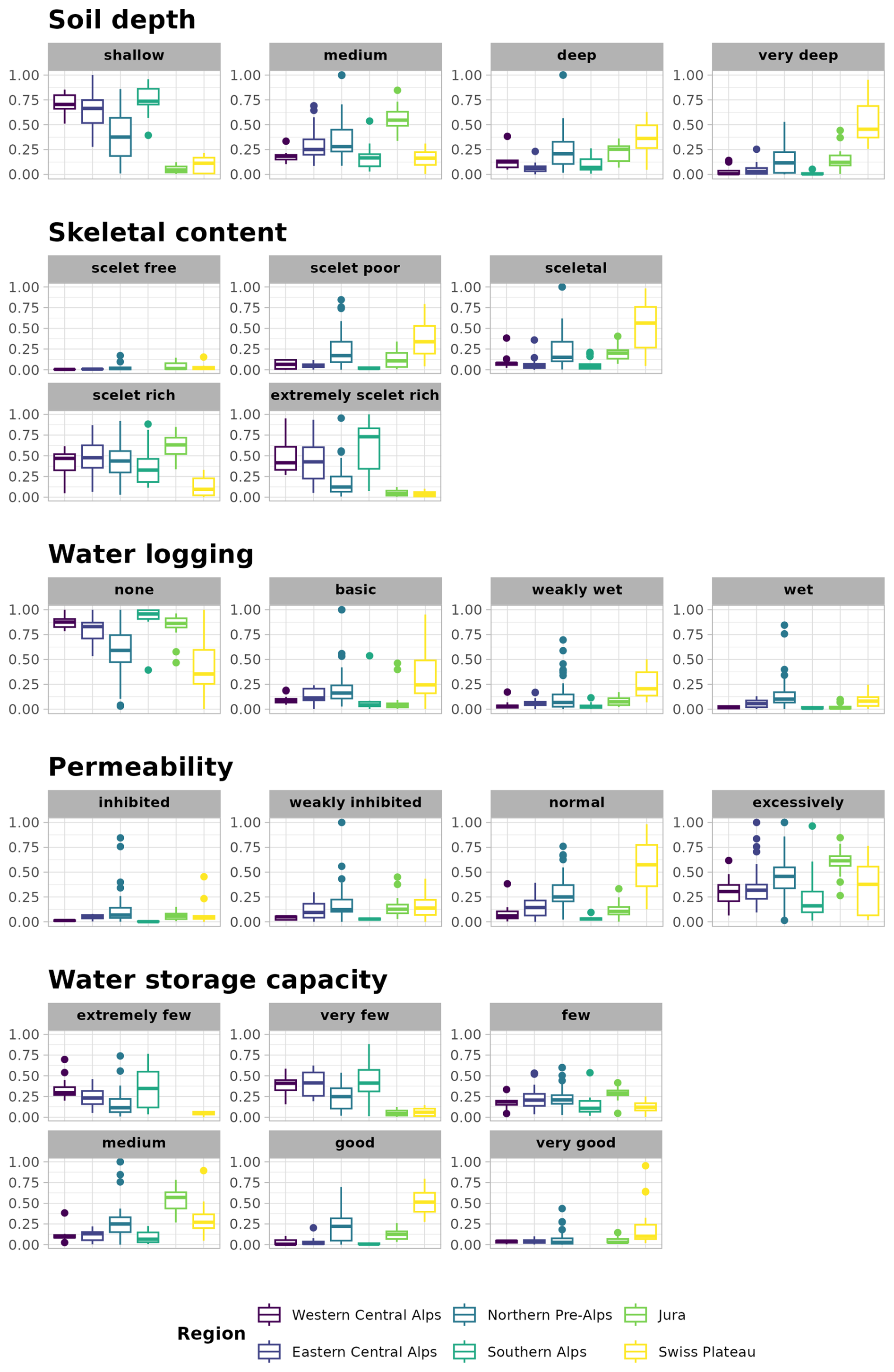
Figure A1 Catchment coverage fractions for all (sub-)categories of the soil characteristics: soil depth, skeletal content, water logging, soil permeability, and water storage capacity across regionalized catchment groups derived from the biogeographic regions of Switzerland (colours, see also Fig. 7a).

As an example application, we show the distribution of catchment coverage fractions across biogeographic regions for the soil characteristics soil depth, skeletal content, water logging, permeability, and water storage capacity (Fig. A1).

The percentage coverage distributions reveal notable differences in soil characteristics and their subcategories. Catchments in the Swiss Plateau region are characterized by larger coverages of deep to very deep soils with a mostly poor to medium skeletal content, normal soil permeability and good water storage capacities (see Fig. A1). Alpine catchments, on the other hand, are characterized by shallower soils (especially the Southern Alps) and a higher skeletal content. Soils in the Alps further have almost no water logging and a low water storage capacity. Soils with a (weakly) inhibited permeability or with a very good water storage capacity are infrequent across all biogeographic regions.

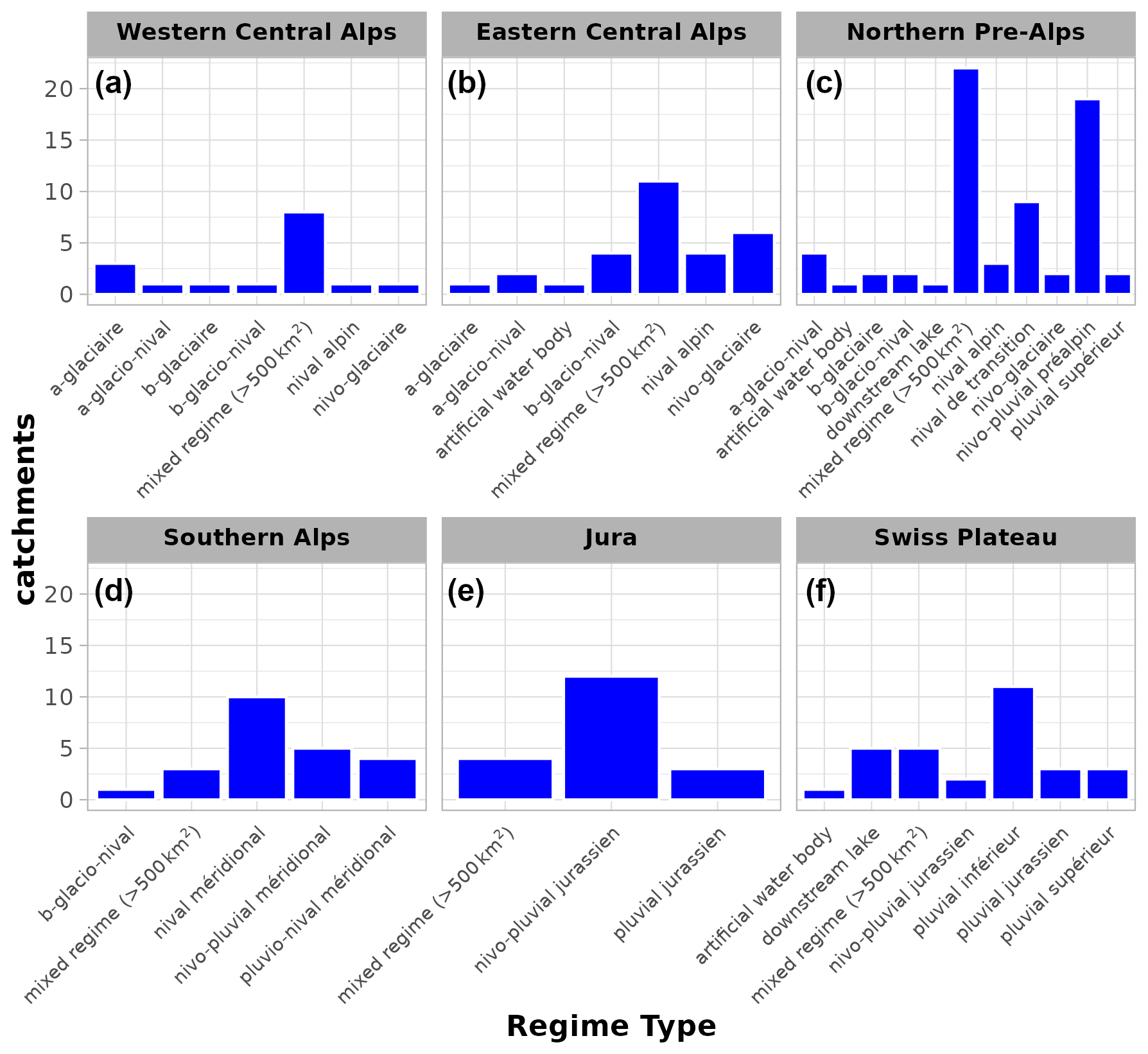
Figure A2 Streamflow regime type incidence among catchments grouped by the biogeographic regions of Switzerland (Western Central Alps, Eastern Central Alps, Northern Pre-Alps, Southern Alps, Jura and Swiss Plateau region; see Sect. 3.3 and also Fig. 7). The streamflow regime type classification was provided by the FOEN. The y-axis shows the number of catchments associated with each category.

Whereas soil characteristics reflect differences in terrestrial catchment characteristics, the streamflow regime types are more indicative of hydro-climatic streamflow generation processes (see Sect. 2, Fig. A2). In Alpine environments, snow- and glacier processes are important contributors to streamflow generation. Hence, both Western and Eastern Central Alps show predominantly glacial and nival streamflow regime types of which 86 % are shared among regions (see Fig. A2a, b). In contrast to the Central Alps, the hydro-climatology of the Southern Alps is more Mediterranean with the Alps often described as “Alpine divide” between the warmer and drier conditions in the South and more temperate Atlantic influences in the North (NCCS, 2025; Haslinger et al., 2019). Despite similar streamflow generating processes, the streamflow regime types in the Southern Alps are differentiated from their counterparts in the Central Alps (méridional, see Fig. A2d) and, in contrast to the Central Alps, can also include stronger contributions of pluvial processes. The Northern Pre-Alps show the largest variability of streamflow regime types (Fig. A2c). As transitional region between Alps and lowlands, streamflow regime types also show a large variety of processes contributing to streamflow generation including glacial, nival and pluvial processes. The Jura is a subalpine mountain range characterized by a strongly karstified geology. The variability of streamflow regime types is the lowest among biogeographic regions and consists mainly of locally specific types (jurassien) influenced by a mixture of nival and pluvial processes (Fig. A2e). The Swiss Plateau region is equivalent to the lowlands and hence is dominated by pluvial streamflow regime types (Fig. A2f).

Note that whereas catchments smaller than 500 km² allow for a more distinct discrimination in streamflow regime types and hence streamflow generating processes, catchments with an area larger than 500 km² are influenced by a multitude of streamflow generating and/or storage processes (e.g., groundwater contributions) and are hence provided as mixed regime (> 500 km²) type (see Sect. 2). The mixed regime type is the most prevalent among catchments (see Fig. 2 and occurs across all biogeographic regions (Fig. A2) being the most frequent regime type in Western and Eastern Central Alps as well as in the Northern Pre-Alps.

The catchment grouping to biogeographic regions presented here is again based on maximum overlap of catchment area with the specific biogeographic region (see also Fig. 7a). Biogeographic regions are frequently used for grouping catchments into groups of similar streamflow (generation) characteristics and provides usable results (see e.g., Brunner et al., 2019b; Muelchi et al., 2021b; von Matt et al., 2024). In specific cases where a categorization into biogeographic regions may not be unambiguous (see Sect. 5.1), categorization may be reconsidered by the user via alternative grouping (e.g. directly on streamflow regime types), alternative categorization approach (other than maximum overlap) or expert judgement. As such the streamflow regime types nivo-pluvial jurassien and pluvial jurassien could for example be recategorized to the Jura region (see Fig. A2f).

A2 Detailed Event analysis

The combination of hydro-meteorological indicators, standardized (drought) indices (SPI, SPEI, SMRI), (potential) cumulative water and streamflow deficits (CWD, PCWD, CQD) and accompanying climatological anomalies allow for a detailed analysis of specific (streamflow) drought events. Drought-generating processes vary across catchments depending on hydro-climatological and terrestrial catchment characteristics, the season as well as on anthropogenic disturbances (e.g., Brunner et al., 2022; Van Loon and Van Lanen, 2012; Van Loon, 2015; Apurv et al., 2017). Except for glacier melt and groundwater, the HYD-RESPONSES dataset provides time series for all relevant hydro-meteorological indicators required to analyse (streamflow) drought generation, drought propagation as well as drought type classification.

Figure 6 illustrates time series for the year 2022 of a subset of relevant hydro-meteorological variables for catchment 2034 – Broye, Payerne, Caserne d'aviation. This catchment is located in the western Swiss Plateau region (highlighted in Fig. A4).

The year 2022 was an exceptional year with unprecedented combined heat and drought conditions over Europe (Tripathy and Mishra, 2023). The Broye catchment experienced low-flow conditions beyond a 100-year return period (BAFU, 2023b). In the Broye catchment, the lowest 7 d average streamflow values were observed between July and August (see Fig. 6i) Several streamflow drought events were identified for both yearly fixed (purple shading) and variable (green shading) threshold definitions (see Fig. 6 (all panels)). The longest events occur during the annual low-flow season for both definitions.

The year 2022 was also one of the warmest years on record with three heatwaves occurring in mid-June, mid-July and in the beginning of August (Imfeld et al., 2022). During the longest streamflow drought event in July 2022 (see Fig. 6i), evaporation anomalies begin to decline and become negative towards the end of the event (see Fig. 6c). Concurrent strong negative soil moisture anomalies at shallow and deeper levels (see Fig. 6d) suggest that the successively decreasing evaporation anomalies may be related to increasingly depleted soil moisture storages resulting in limited water availability for evaporation. Interactions between (subsurface) storage processes are however complex and also include groundwater–soil moisture interactions (e.g., Orth and Destouni, 2018).

The HYD-RESPONSES dataset further provides information on cumulative (atmospheric) water deficits represented by standardized and non-standardized (drought) indices.

For the Broye catchment, the 2022 streamflow drought events identified with the variable threshold (green shading) correlate well with shorter aggregation scales (1- to 3-monthly) SPI and SMRI indices in spring and summer. The correspondence between short-term precipitation deficits and streamflow droughts is, however, not consistent throughout the year. During the variable threshold streamflow droughts in mid-March to April, both SMRI-1 and SMRI-3 reach more negative values than their SPI equivalents, which indicates that lacking snowmelt contributed to the streamflow drought generation (see Fig. 6g, h). Lacking snowmelt as contributing factor is further confirmed by considering the larger and rather persistent negative anomalies in both SWE and snowmelt in the preceeding 1 to 3 months (see Fig. 6e, f).

Cumulative deficits in actual (CWD, Fig. 6k) and potential (PCWD, Fig. 6l) water balance as well as streamflow (CQD, Fig. 6j) provide complementary information to the SPI, SMRI and SPEI in the form of non-standardized and hence physically interpretable deficit amounts.

Cumulative streamflow deficits (CQD) show only two phases without deficit compensation for both drought definitions (Fig. 6j). A shorter CQD phase coincides with the drought events in spring (variable threshold) and the shorter drought event in June (fixed threshold), while a longer phase coincides with the remaining shorter and longer streamflow drought phases in July and August before CQD is compensated by September 2022. For both CQD phases, the CQD is larger for streamflow droughts based on a variable threshold definition. Above average precipitation (+130 %; BAFU, 2023b) was reported in September 2022 and corresponds well with the compensation of CQD and is also reflected in the positive monthly (31 d) precipitation anomalies (P anomaly, Fig. 6b).

Similar to the longest streamflow drought phases, also the largest cumulative deficits in water balance (CWD) occurred between May–August 2022 (in terms of both absolute deficits and anomalies, see Fig. 6k, m). Based on the seasonal climatology of both temperature and evaporation (highest values during summer), larger absolute CWDs are generally expected to occur during the warm season (not shown). Major CWD phases match streamflow drought phases remarkably well, especially for the variable threshold definition with one exception in April. The two longer streamflow drought phases in May–June further show the benefits of considering anomalies in the CWDs. While absolute CWDs were not compensated in between the streamflow droughts, the CWD anomalies indicate that the deficits returned to seasonal norm values (see Fig. 6m). Cumulative deficits in potential water balance (PCWDs, Fig. 6l) are more similar to cumulative streamflow deficits for the variable-threshold definition (CQD, Fig. 6j (blue line)). This reflects the different nature of CWDs and PCWDs. Deficits based on the actual water balance (P–E) are more strongly tied to the actual water availability and hence the individual streamflow (drought) phases (Fig. 6i, k). The potential water balance (P-PET), on the other hand, represents the deficit that would have been accumulated under unlimited water availability. Similar to PCWD, CQDs reflect the integrated streamflow deficit over time while an actual deficit in terms of low streamflow levels does not necessarily have to exist (anymore).

A3 Composite analysis (catchment response patterns)

Composite analysis is a frequently used approach to understand the driving processes of a phenomenon such as droughts (see e.g., Bevacqua et al., 2021; Floriancic et al., 2020; Mahto and Mishra, 2024). By considering the median values of drought indicators across all streamflow drought events in a catchment, typical response patterns may become more evident and may allow for more generalized inferences on typical streamflow drought response patterns e.g., to precipitation deficits accumulated over various aggregation time-scales. Here, we present a composite analysis of median SPI values associated with streamflow droughts defined by the monthly 15th-percentiles of the streamflow which corresponds to the highest of the low-flow percentile used for the Swiss national drought platform (see BAFU, 2025).

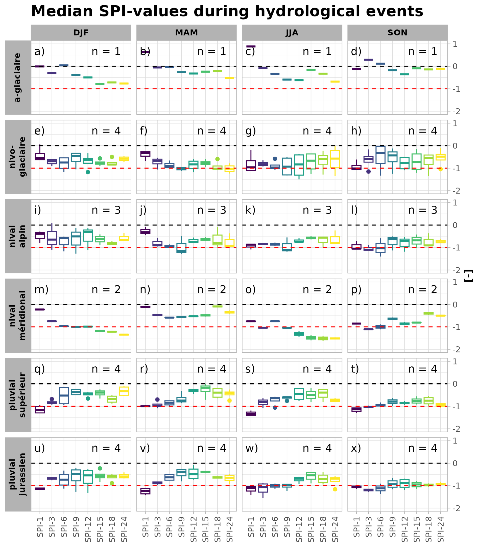
Figure A3 Median SPI values during hydrological drought conditions for all events of all catchments for six selected streamflow regime types across the four seasons winter (DJF), spring (MAM), summer (JJA) and autumn (SON). The streamflow regime types were selected to represent catchments with (dominant) glacial (a-glaciaire, nivo-glaciaire), snow (nival alpin, nival méridional) and pluvial processes (pluvial jurassien, pluvial supérieur) and spatial diversity. Hydrological drought events were defined by a moving monthly (31d) 15th-percentile (variable) threshold. Boxplots are coloured according to SPI aggregation time scales (1- to 24-months). Moderate drought conditions are indicated by the red dashed lines, the black dashed line indicates 0. “n=” refers to the number of catchments with a specific streamflow regime type.

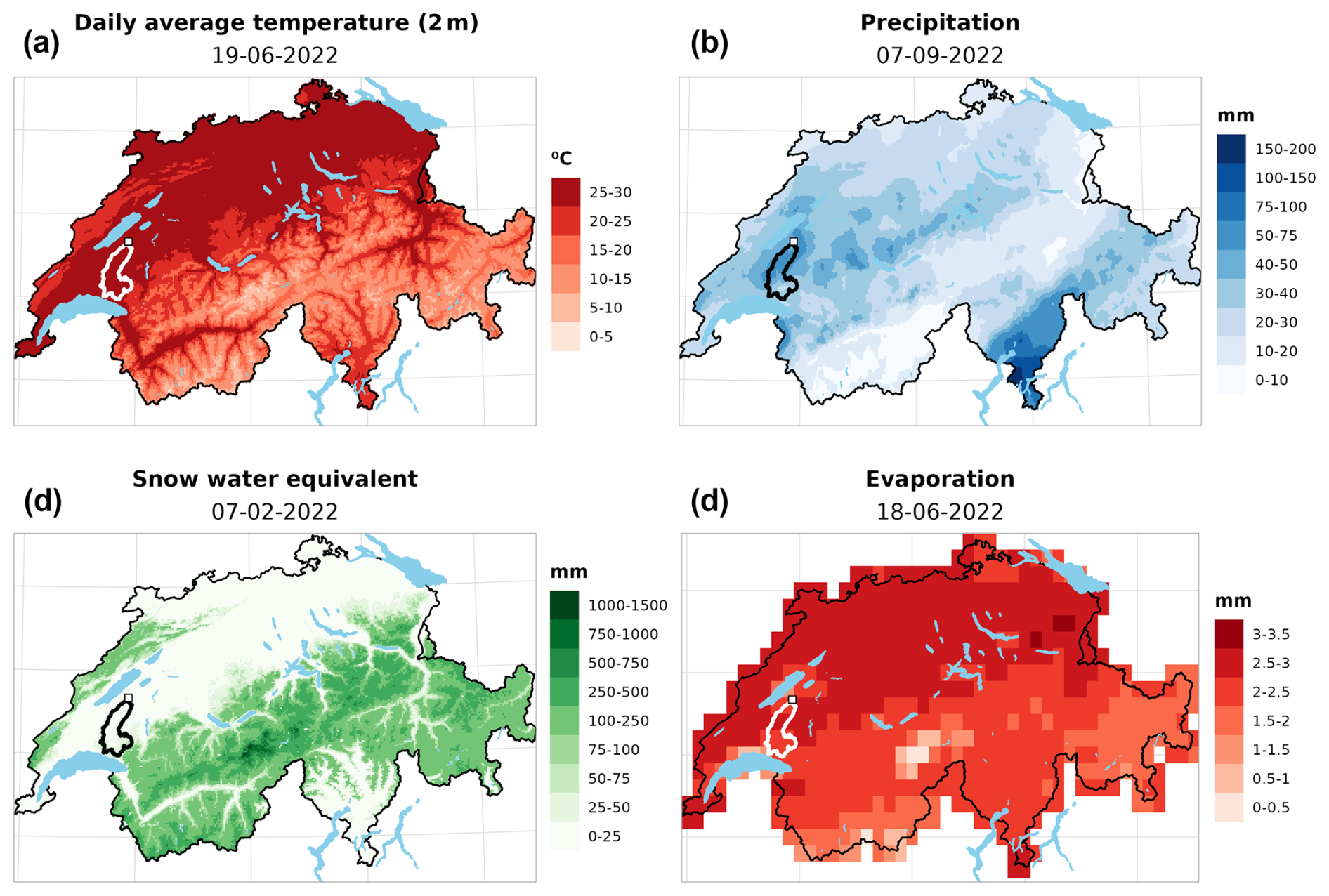
Figure A4 Overview of the spatial raster products used to extract daily time series. (a) Mean daily temperature (TabsD, MeteoSwiss), (b) Daily precipitation sun (RhiresD, MeteoSwiss), (c) Daily snow water equivalent of the Swiss snow climatology (SPASS) (SWE, MeteoSwiss & SLF), (d) Daily evaporation sum (aggregated from hourly ERA5-Land data, ECMWF). Note that the second snow climatology product (OSHD) is not shown. Contours in white/black show catchment 2034 – Broye, Payerne, Casernde d'aviation for the day with the highest observed catchment average values for each specific product for the year 2022. White squares show the catchment outlet where daily streamflow is measured. Extracted and derived time series over the year 2022 are shown for the same catchment in Fig. 6.

Note that streamflow drought characteristics and drought propagation processes may differ among catchments depending on hydro-meteorological climatologies, geological and terrestrial characteristics (e.g., aquifer, rock type, (soil) water storage capacity), seasonality of and differences in contributing streamflow (drought) generating processes and human disturbances (e.g., Van Loon and Laaha, 2015; Floriancic et al., 2022; Jehn et al., 2020; Apurv and Cai, 2020; Savelli et al., 2022; Haile et al., 2020; Brunner et al., 2022, 2021, 2023; Tijdeman et al., 2022; de Jager et al., 2022). We therefore separate the streamflow droughts and catchments by seasons winter (DJF, December–February), spring (MAM, March–May), summer (JJA, June–August) and autumn (SON, September–November) and by streamflow regime types. Six streamflow regime types are selected to capture a variety in dominant streamflow (drought) generating processes. These include glacial (a-glaciaire, nivo-glaciaire), nival (nival alpin, nival méridional) and pluvial (pluvial jurassien, pluvial supérieur) processes. The importance of precipitation deficits across scales is assessed using SPIs (SPI-1 to SPI-24). Streamflow drought events are only considered for the longest common homogeneous period across catchments (1991–2022). The selection is further restricted to catchments with at least 10 streamflow drought events in each season (over the entire time series length) with a minimum duration of at least 10 d to enhance robustness and exclude minor droughts.

Median SPI values are mostly negative across all aggregation time-scales indicating that precipitation conditions co-occuring with streamflow droughts tend to be drier than normal. Several streamflow regimetype-specific response patterns are evident and change across seasons along with contributing streamflow (drought) generating processes.

Glacier melt is the dominant factor for the a-glaciaire regime type (Fig. A3a–d). Streamflow levels are typically lowest in winter (January–March) as a result of precipitation falling as snow (intermediate storage) and highest in summer due to large contributions of glacier melt (Aschwanden and Weingartner, 1985; Weingartner and Schwanbeck, 2020; Muelchi et al., 2021b). Streamflow droughts of strongly glaciated catchments are not associated with moderate drought conditions at any SPI scale. In glacial and nival catchments a shift towards short-term precipitation deficits (SPI-1 to SPI-6) being associated with droughts is present across seasons and drought-generating processes. The transition towards shorter deficit scales emerges in summer for nival regime types (Fig. A3g, k) and in autumn for glacial regime types (Fig. A3d). In pluvial and transitional regime types short-term precipitation deficits (mostly 1- to 3 months) are relevant throughout the year (Fig. A3q–x). Seasonal shifts are also observed for pluvial and transitional regime types with mid- and long-term precipitation deficits becoming more relevant in summer and autumn (Fig. A3t, w–x).

In addition to 3-monthly precipitation deficits, also mid- and long-term deficits become relevant in summer and autumn for (nivo-pluvial) catchments in the Jura region and catchments of the regime type pluvial inférieur (Fig. A3s, t). Compound moderate droughts are mainly observed for sub-yearly (1- to 9-monthly) scales with most extreme conditions on a 6-monthly scale in the Jura region (especially for nivo-pluvial catchments) and on a (6- to) 9-monthly scale for catchments of the regime type pluvial inférieur. In southern Switzerland, precipitation deficits tend to be relevant on longer scales compared to similar regime types north of the Alps (Fig. A3m–p). In contrast to nival catchments north of the Alps (nival alpin, Fig. A3i–l), droughts in the nival catchments south of the Alps (nival méridional, Fig. A3m–p) are associated with substantial precipitation deficits at longer aggregation times (9–24 months). The deficits occur in winter and in summer, but conditions are more extreme in summer (SPI $\approx -\mathrm{1.5}$) on scales longer than 15 months. Further, also 3-monthly precipitation deficits appear to be relevant for streamflow (drought) generation in summer (moderate drought conditions). In spring and autumn, mid- to short-term accumulation scales are more relevant (Fig. A3). Interpretations of the differences between the south and north sides of the Alps should,however, be considered with caution due to the small catchment sample sizes and the spatial proximity of the two nival méridional catchments. The observed response patterns may therefore not be representative of nival catchments south of the Alps in general.

Appendix B: Tables

Table B1 Glossary of extracted time series variables, their description and units.

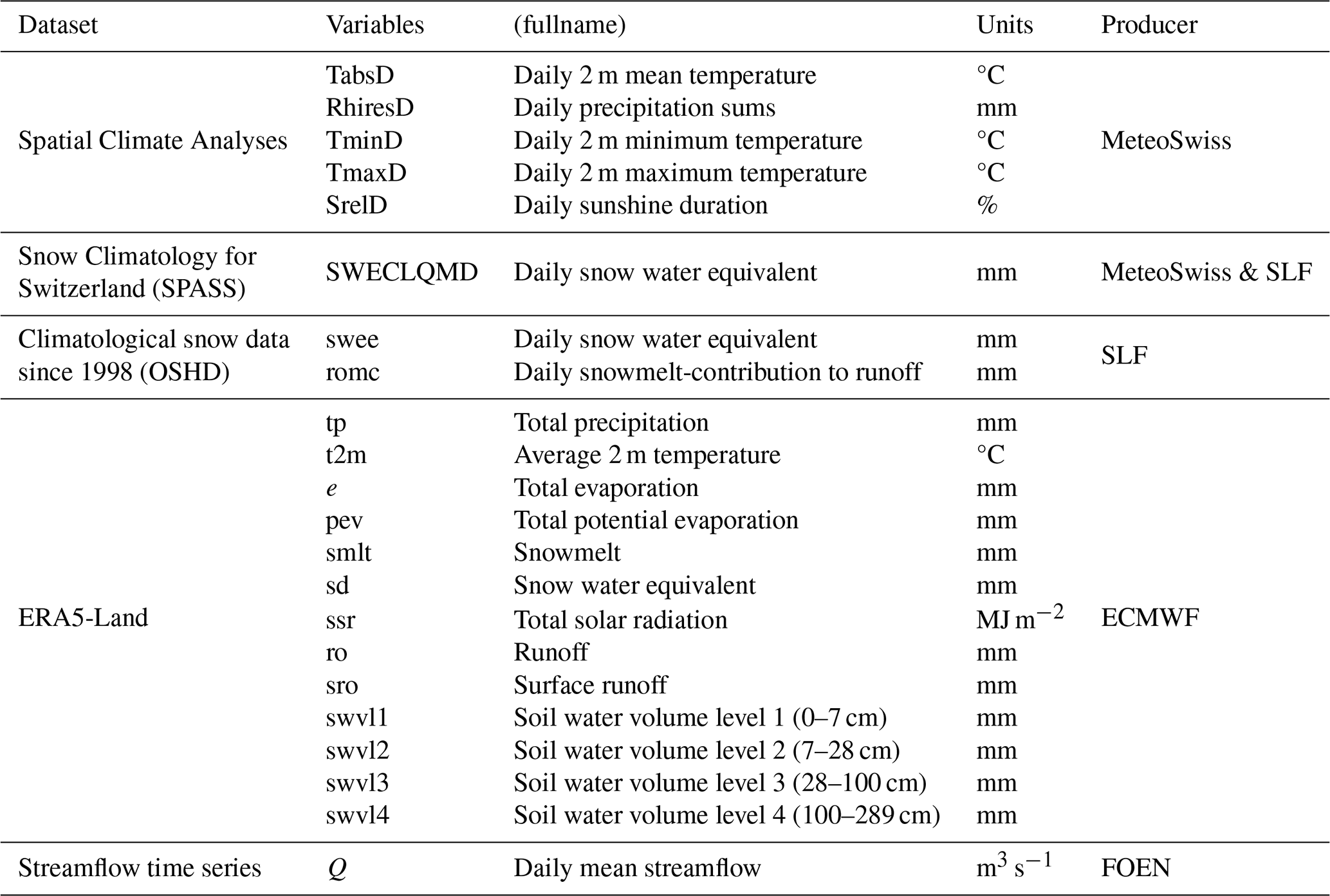
Table B2 Information on the underlying processing and reliability of basic and derived time series variables.

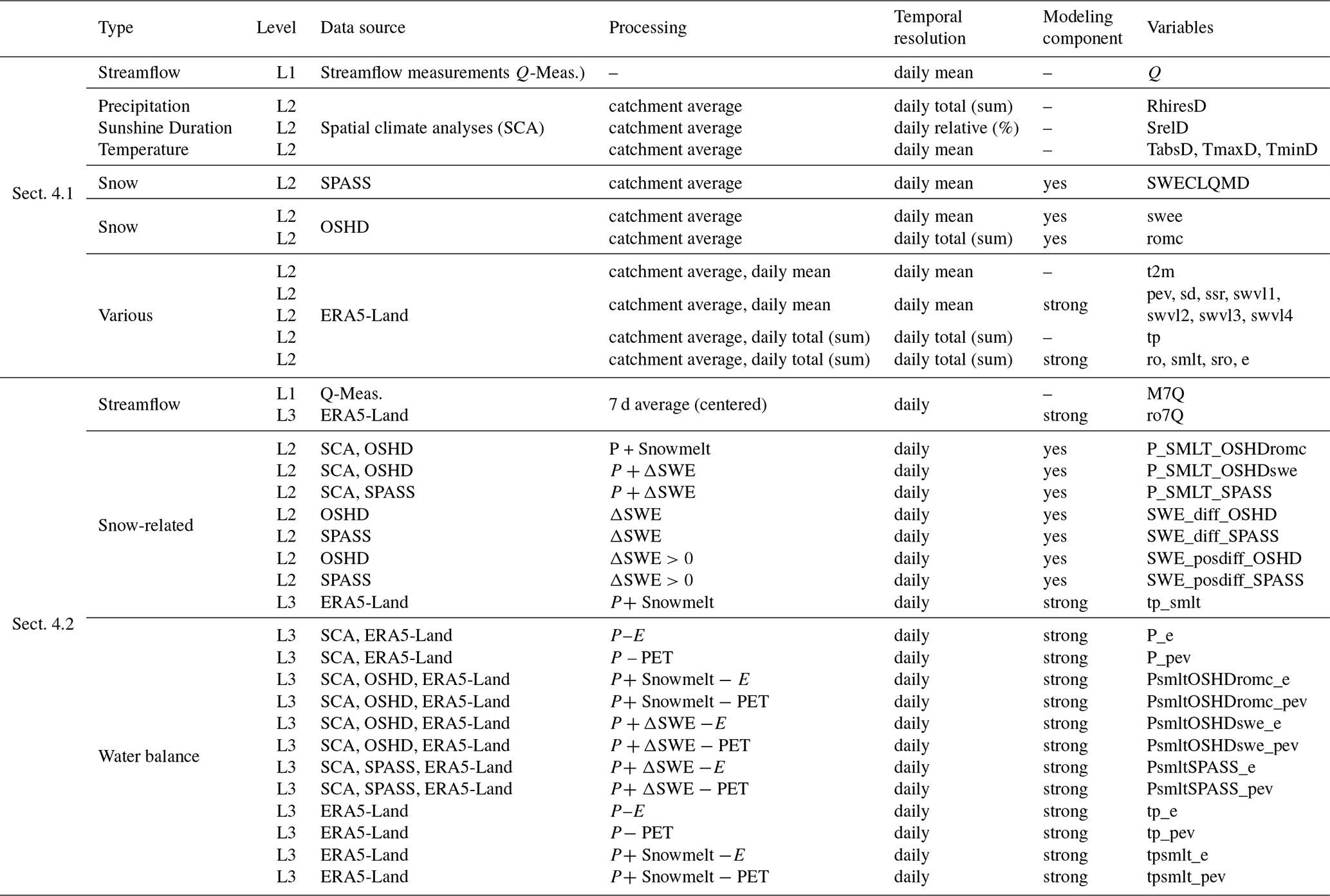
Table B3 Information on the underlying processing and reliability of standardized (drought) indices and cumulative deficit time series.

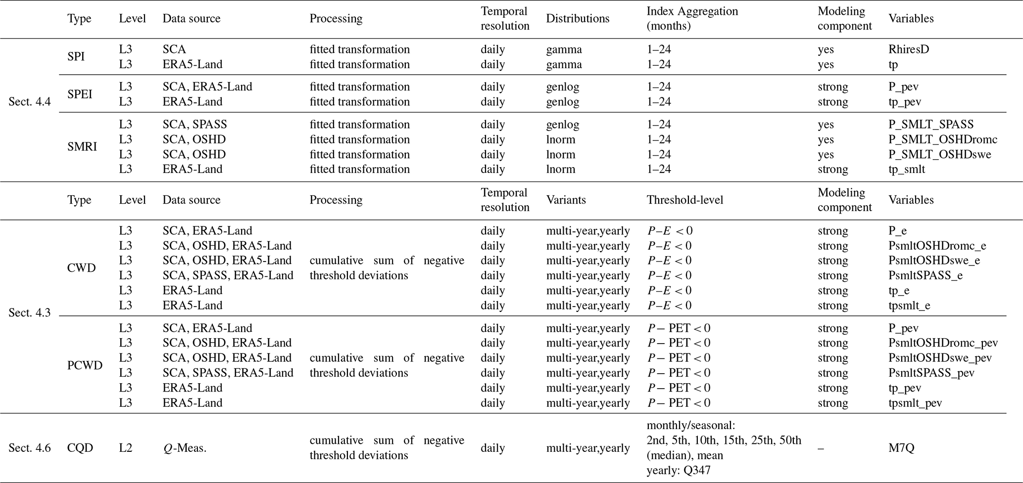
Table B4 Information on the underlying processing of the climatology and anomaly time series.

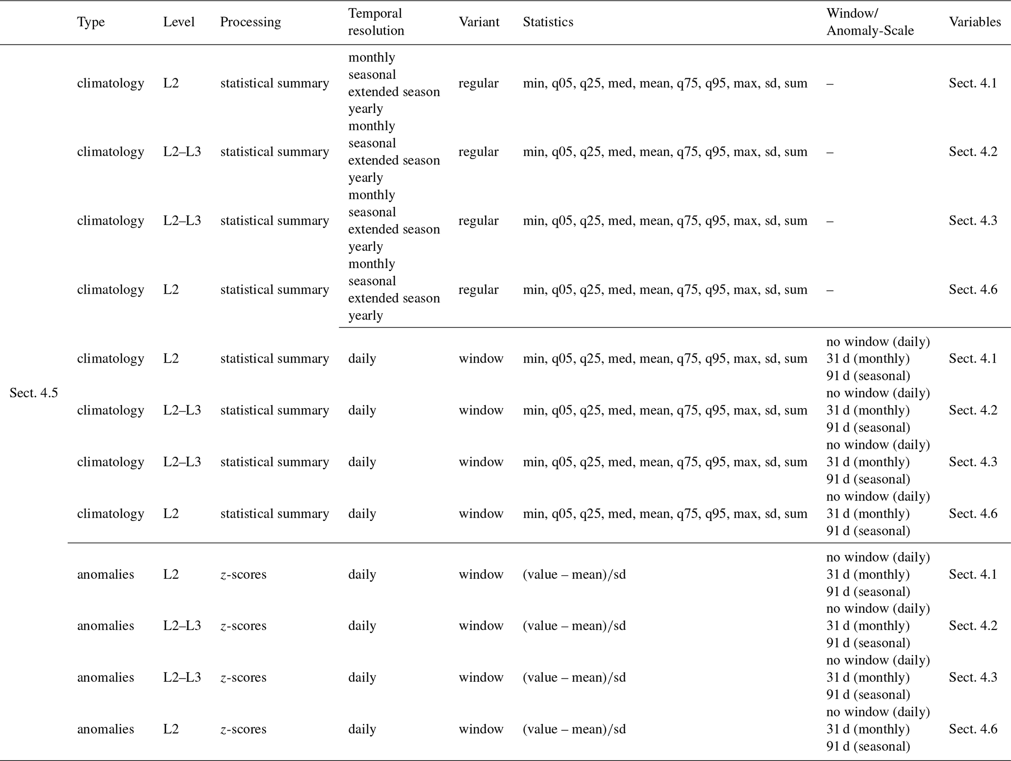
Table B5 Information on the underlying processing and reliability of event time series.

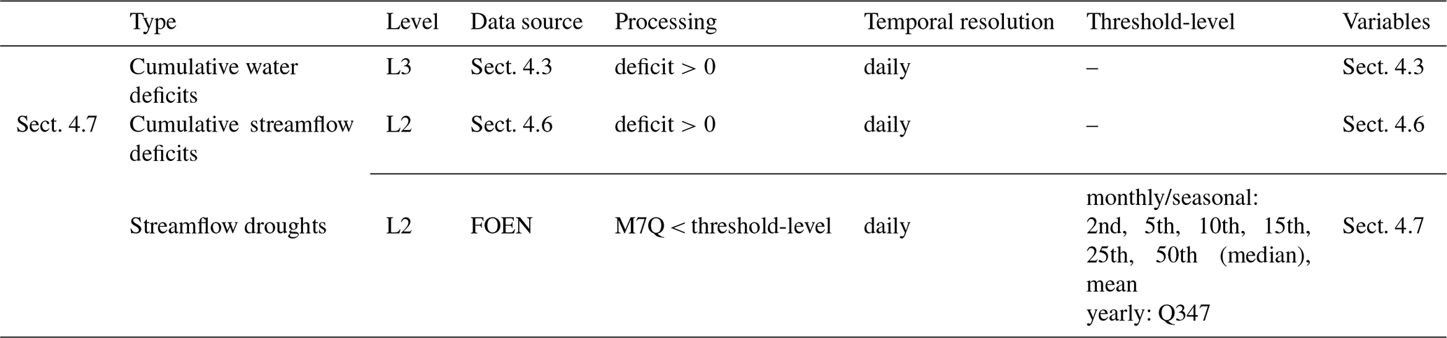
Table B6 Characteristics of all 184 catchments in the HYD-RESPONSES dataset (Part 1/5).

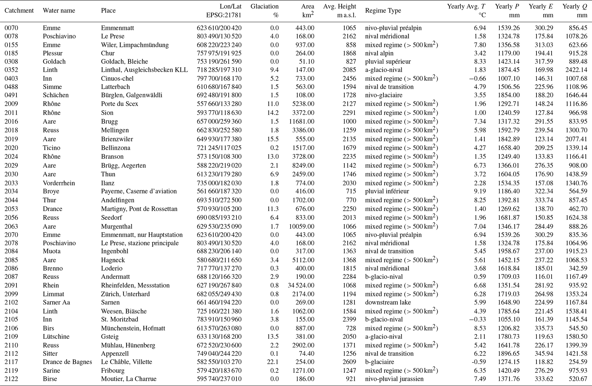
Table B7 Characteristics of all 184 catchments in the HYD-RESPONSES dataset (Part 2/5).

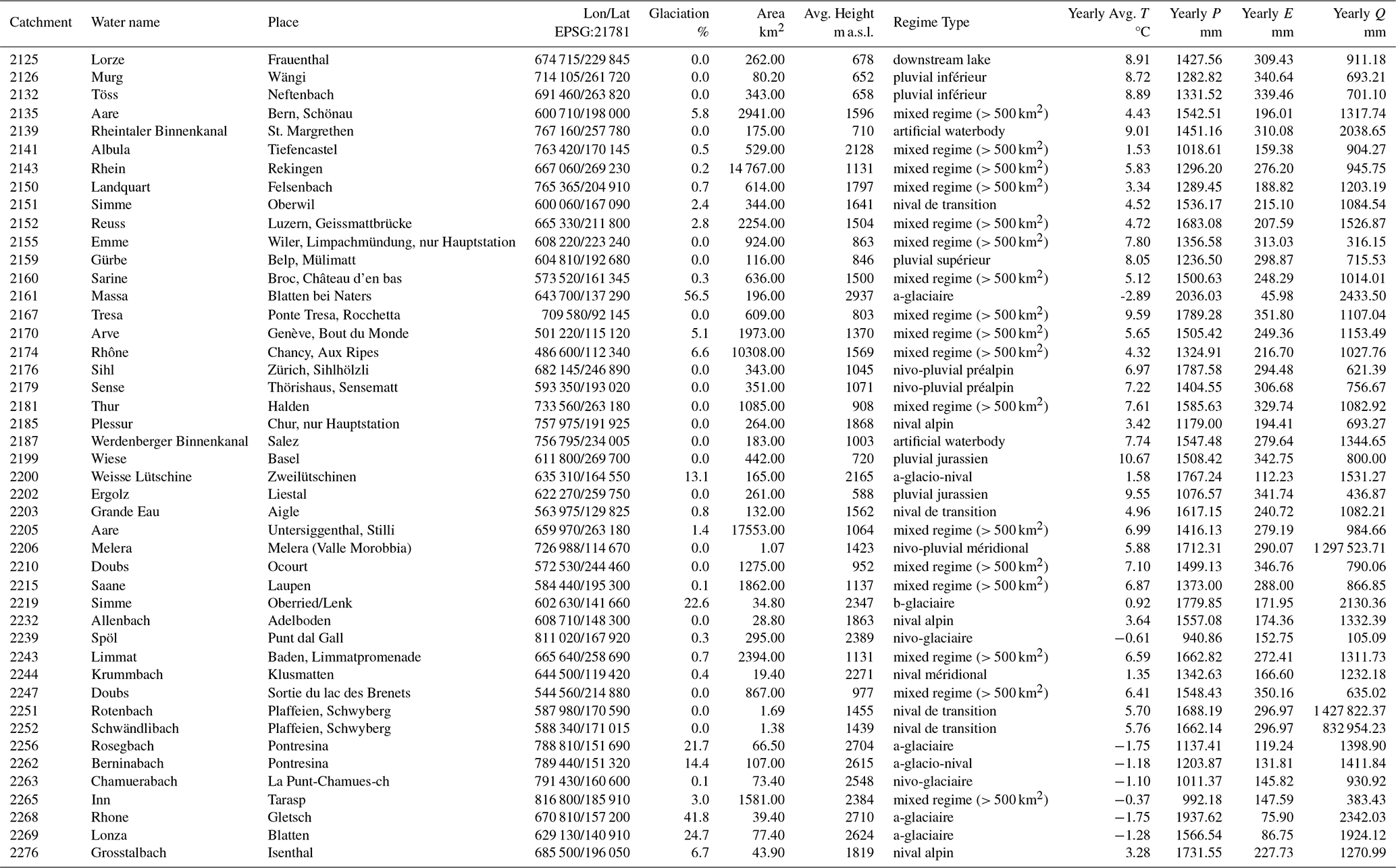
Table B8 Characteristics of all 184 catchments in the HYD-RESPONSES dataset (Part 3/5).

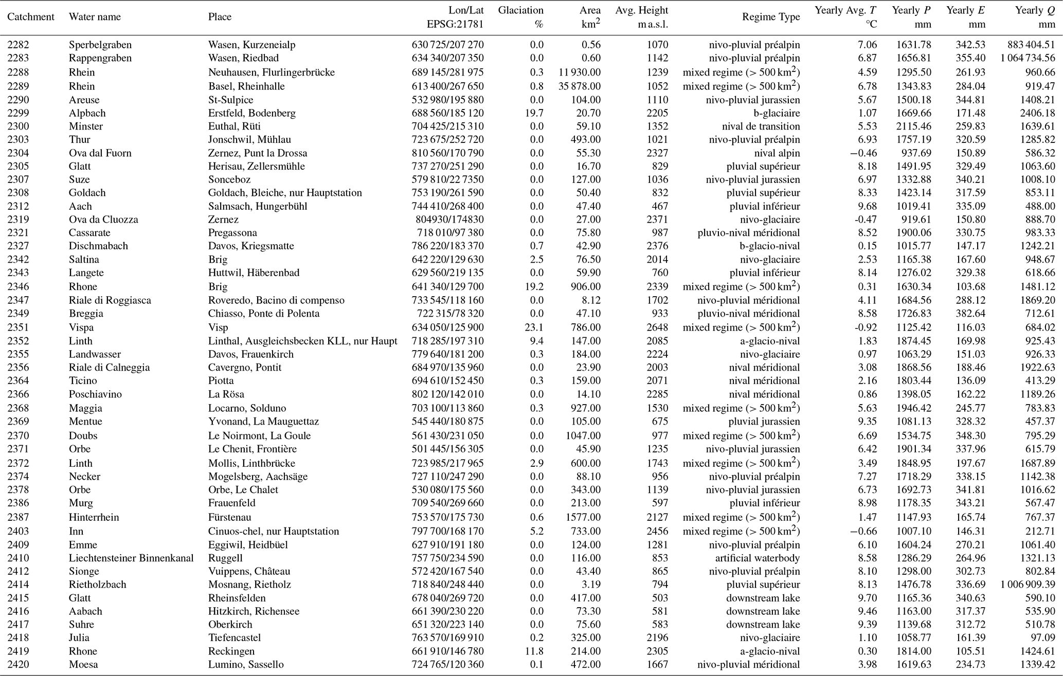
Table B9 Characteristics of all 184 catchments in the HYD-RESPONSES dataset (Part 4/5).

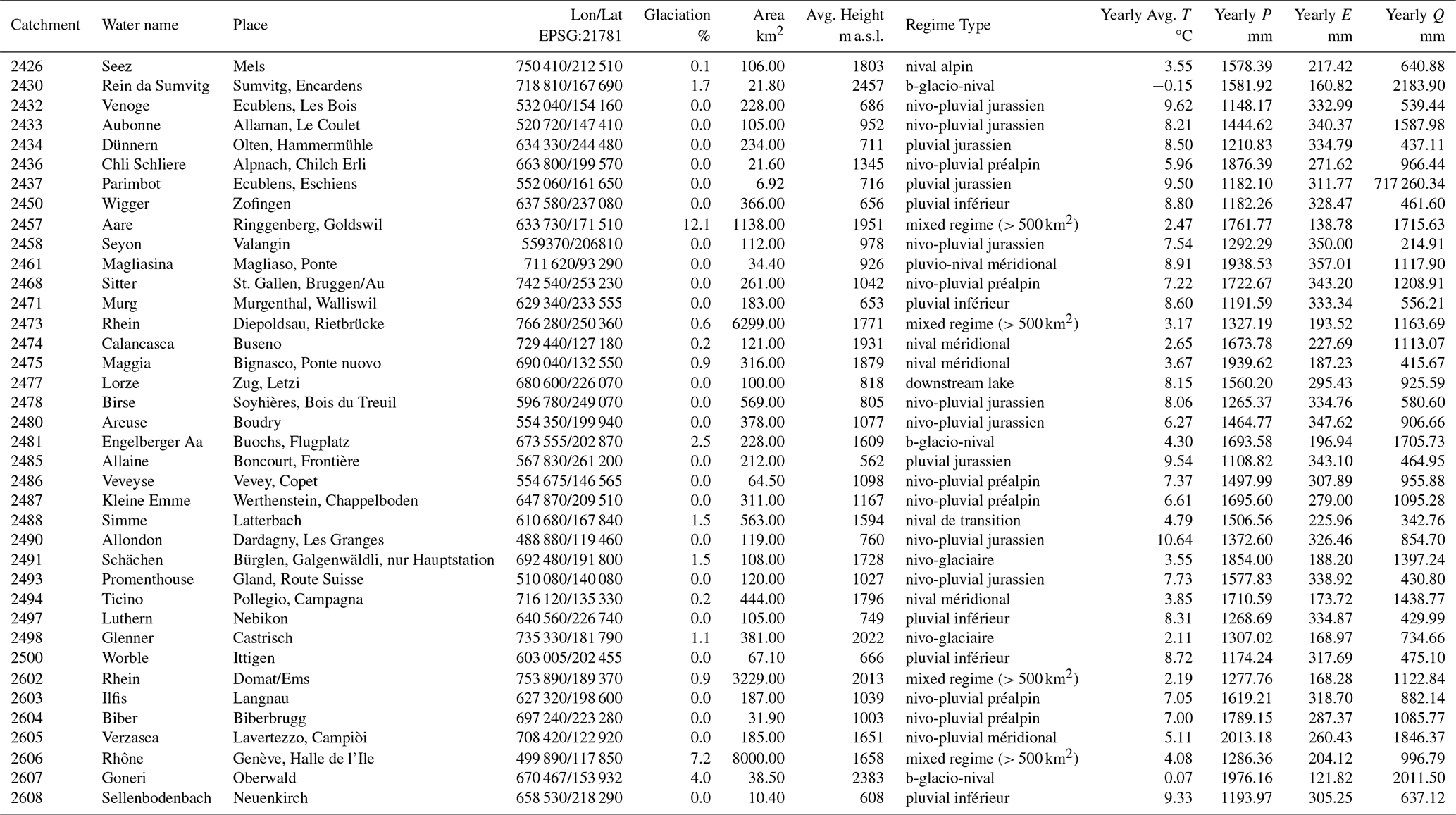
Table B10 Characteristics of all 184 catchments in the HYD-RESPONSES dataset (Part 5/5).

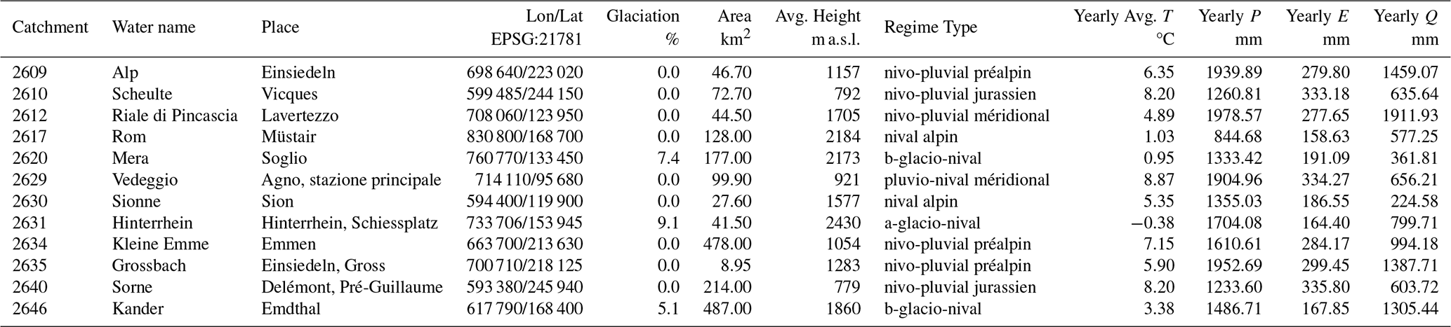
T= Temperature, P= Precipitation, E= Evaporation, Q= Streamflow/Runoff