A daily gridded high-resolution meteorological data set for historical impact studies in Switzerland since 1763

High-resolution gridded daily data are needed to study historical climate and weather impacts. Current daily gridded data sets in Switzerland extend to 1961 or 1971 for variables such as minimum and maximum temperature and sunshine duration. However, studying historical weather and climate events, such as the year-without-a-summer requires much longer time periods. For Switzerland, high-resolution gridded reconstructions of daily mean temperature and daily precipitation sums have recently been developed based on a large amount of early instrumental data for a period from 1763 to 1960. Here, we present an extension of these daily reconstructions to six more variables, namely, relative sunshine duration, relative humidity, minimum and maximum temperature at 2 m, and u- and v-wind at 10 m with a 1 × 1 km resolution. These additional reconstructions are based on the same method as the previous reconstructions by combining the analogue resampling method and data assimilation. Cross-validation results using a network representative of early 19th-century observations show a mean squared error skill score ranging from 0.70 to 0.80 for wind speed, depending on the season. For maximum and minimum temperature, values average between 0.48 to 0.82, depending on the seasons. These results indicate reasonable skill of the reconstructions and show that the wind and temperature fields outperform climatology despite the data scarcity in the historical period. However, for relative humidity and relative sunshine duration, the values of the mean squared skill score are significantly lower, ranging between −0.31 to 0.48. Furthermore, we explored the potential of the extended reconstructions by evaluating two historical and one contemporary wildfire events in Switzerland using the widely applied Canadian Forest Fire Weather Index (FWI). The two historical summer fires were associated with a notably high fire danger in the reconstruction. For the contemporary winter fire, the reconstruction agrees well with the index calculated from the COSMO-1 weather forecast model, although neither indicates exceptionally high fire danger.

Overall, this is the first dataset that enables impact studies of weather and climate in Switzerland, reaching as far back as 1763. The datasets are freely available at the BORIS repository of the University of Bern: https://doi.org/10.48620/87086 (Imfeld and Brönnimann, 2025).

1 Introduction

Long-term high-resolution reconstructions of meteorological variables are crucial for studying historical climate variability, understanding the occurrence of past extremes, and assessing their impacts on, for example, hydrology and agriculture. Over the past years, significant data rescue efforts uncovered numerous observational records for the 18th and 19th centuries that are, however, sparse in spatial coverage (e.g., Brugnara et al., 2015, 2020). While gridded data sets for daily mean temperature, daily precipitation sums, or daily mean pressure have been reconstructed from such rescued records for Switzerland (Pfister et al., 2020; Imfeld et al., 2023) and Europe (Pappert et al., 2022; Schmutz et al., 2024), gridded data sets for other important variables – such as wind speed, humidity, sunshine duration, and minimum and maximum temperatures – are very scarce for long-term historical periods. For example, dynamical downscaling approaches have been used to study a variety of variables for specific extreme events on hourly to daily scales (e.g. Stucki et al., 2015, 2024; Michaelis and Lackmann, 2013), but no continuous long-term daily gridded data exist except for the 20th century reanalysis with a rather coarse resolution (Slivinski et al., 2019). This is primarily due to the lack or limited availability of measurements, which often suffer from questionable representativeness or quality (e.g., wind measurements taken on church towers). Yet, these variables are crucial for assessing, for example, agricultural impacts, drought conditions, and ecosystem responses.

In this study, we extended the existing daily reconstruction of mean temperature and precipitation sums (Imfeld et al., 2023) to include the u- and v-wind component at 10 m, mean and minimum daily relative humidity, daily relative sunshine duration, and minimum and maximum temperatures at 2 m covering the period 1763 to 2020. To ensure consistency with the previous reconstruction, we used the same set of observations and adhered as closely as possible to the original methodology. Our primary focus was on providing fields for 10 m wind and daily maximum and minimum temperature at 2 m, for which we performed data assimilation on top of the analogue resampling. The other variables, mean and minimum relative humidity and daily relative sunshine duration, are included in the data set because they are frequently requested, particularly for applications like crop modeling or fire weather conditions; however, these variables are solely based on the analogue resampling without additional data assimilation.

The reconstructed variables enable the calculation of indices such as the Canadian Forest Fire Weather Index, providing insights into historical fire weather conditions. To demonstrate the utility of the data set, we used two historical forest fire events in Switzerland (late summers of 1911 and 1943), complemented with documentary sources, to showcase its potential for analyzing past events and their impacts, as well as a modern event in the winter of 2016 to compare it to a modern weather forecast model.

The paper is organized as follows: Sect. 2 presents the observations and gridded data sets used for the reconstruction. In Sect. 3, we describe the methodology of the reconstruction, and in Sect. 4, we show the corresponding validation results. Section 5 discusses the consistency and uncertainty of the variables, and Sect. 6 shows a use case of the data sets. Conclusions are drawn in Sect. 7.

2 Data

2.1 Instrumental data

Our reconstruction method requires both historical measurements and corresponding present-day observations from the analogue reference period. For our new reconstructions, we largely relied on the same set of observational records detailed in depth in the first article (Imfeld et al., 2023), but additionally included observations for daily minimum and maximum temperature for the period since 1864. Therefore, we provide here only a brief description of the observational records.

2.1.1 Historical period

The reconstruction period can be divided into two periods, from 1763 to 1863 and from 1864 to 2020 (including the reference periods). For the period before 1864, we relied on early instrumental data rescued through various initiatives (Camuffo and Jones, 2002; Klein Tank et al., 2002; Füllemann et al., 2011; Brugnara et al., 2020; Pfister et al., 2019; Brugnara et al., 2022). These early instrumental data required more pre-processing because standardized measurement practices were not yet established at the time of recording, resulting in inherent limitations in the records. For the reconstructions, we only included time series that passed basic quality controls with a minimum record length of at least seven continuous years and few data gaps. In the early periods of the reconstruction, the network coverage was much sparser, and over time, considerable changes occurred. The changes in the network are depicted in Fig. 1a. At the start of the reconstruction period in 1763, around 11 to 12 series were available (Fig. 1b), which increased to around 30 series in the mid-19th century (Fig. 1c). We refer to these two networks of observations as network 1 (NW1) and network 3 (NW3) as in Imfeld et al. (2023). To increase the number of observations in the early period, we also added time series from nearby locations in Italy and Germany. In total, the reconstruction before 1864 is based on 17 pressure series, 18 temperature series, and 6 precipitation and precipitation occurrence series. Because only very few precipitation measurements were available, we included precipitation occurrence derived from weather notes. All observations underwent standard quality control procedures of daily mean values as implemented in the R-package “dataresqc” (Brugnara et al., 2019), and we performed an additional spatial quality control following Estévez et al. (2018). Temperature and pressure series were homogenized with the paleo-reanalysis EKF400v2 (Valler et al., 2022) as a reference series using the penalized maximal t-test (Wang et al., 2007) and the penalized maximal F-test (Wang, 2008) for break point detection. For the four main cities in Switzerland, Bern, Zurich, Basel, and Geneva, the merged series from Brugnara et al. (2022) were used.

For the later period, starting in 1864, the Swiss National Weather Service MeteoSwiss provides a dense, high-quality, and homogeneous network for daily mean, maximum, and minimum temperature and daily precipitation sums, as well as observations for daily mean pressure for Switzerland (Begert et al., 2005, 2007; Füllemann et al., 2011). These observations form the basis for our reconstruction between 1864 and 1970/2015 and for the reference period between 1971/2016 and 2020. The temperature and precipitation observations meet a high-quality standard, including homogenization, and required no additional processing. For the reconstruction of minimum and maximum temperatures, we used only series without large gaps in the records. For the wind reconstruction, we selected a subset of stations that showed the best validation results for the analog resampling method, and instead of daily precipitation sums, we only used daily precipitation occurrences. The respective networks for the temperature and wind reconstructions are displayed in Fig. 1d–e. We refer to these networks as NW5 for the respective variable. The daily pressure observations, however, also showed quality problems for the period after 1864, including climatic outliers, inhomogeneities, and repetition of values. Therefore, we applied the same methods to the pressure data after 1864, as mentioned above for the early instrumental data. We performed a more profound quality control using the dataresqc R-package (e.g., test for daily repetition, climatic outliers, duplicates, internal consistency) and a spatial quality control comparing estimated pressure to the measured values nearby as done in Estévez et al. (2018). All flagged values were manually checked. When an observation was available in the online weather archive of MeteoSwiss (e.g., MeteoSwiss, 1868), we checked whether these flagged values were digitization errors. We re-digitized 361 pressure values where the error could be attributed to the digitization process. Furthermore, we re-estimated 190 values flagged by the spatial quality control to avoid losing relevant daily data, for example, when a possible digitization error was suspected, but the original document was not available. In addition, 38 values were flagged as climatic outliers; these did not appear in the automated tests from the dataresqc R-package but were physically implausible based on the spatial tests. All flagged values were excluded from the reconstruction, except for those identified as daily repetitions. We homogenized the quality-controlled series using surface pressure from the closest grid point of the ModERA reanalysis (Valler et al., 2024) as a reference series. The break point detection was performed with the penalized maximal t-test (Wang et al., 2007) and the penalized maximal F-test (Wang, 2008). Only break points that were significant without metadata were considered. This simple procedure led to more homogeneous wind reconstructions. We believe that a high-level quality control, involving the use of original documents to verify outliers, identify potential re-digitisation needs, and compile metadata for homogenisation, could lead to further improvements in the pressure time series. This was, however, beyond the scope of this study.

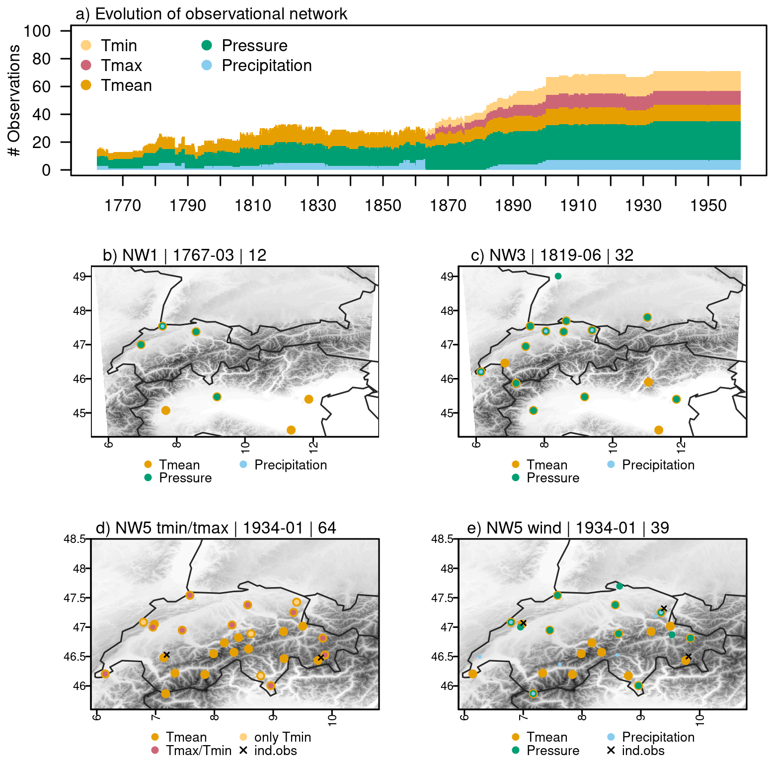
Figure 1 (a) Evolution of available observations between 1763 and 1960. (b) Locations of stations in the network NW 1 in 1767, (c) locations of stations in network NW 3 in 1819, (d) locations of stations used for the reconstruction of maximum and minimum temperature in 1934, (e) locations of stations used for the reconstruction of wind fields in 1934. NW 1 and NW 3 are identical to the networks used in Imfeld et al. (2023) (see Fig. 1 therein). The date in the headings indicates the year for which the network is representative, while the number corresponds to the available observations for that time step. A black cross indicates that measurements from this station have been used for an independent evaluation (tmin/tmax and wind speed). Note that panel (a) shows considerably fewer observations than in Imfeld et al. (2023), because evaluations showed that using fewer precipitation observations led to better results.

2.1.2 Reference period

Each historical observation requires a corresponding counterpart in the reference period. If no reference station was available at the location of a historical station, we used the closest grid point from the daily temperature and precipitation fields or, for sea level pressure, from the European EOBS data set v23.1 (Cornes et al., 2018) during the reference period. For time series in Germany and Italy, if available, we used daily ECA&D station data (Klein Tank et al., 2002), and otherwise the closest grid points from EOBS. All reference series were gap-filled with a quantile mapping approach between the series and a gridded data set (mainly EOBS) following Gudmundsson et al. (2012) and were homogenised if this has not been done yet with nearby stations.

2.1.3 Independent observations

To independently evaluate the temperature reconstruction, we used the two homogeneous minimum and maximum temperature records from Segl Maria and Col du Grand St-Bernard, which were not included in the reconstruction process because they had large gaps in the early 20th century (see asterisks in Fig. 1b). For the wind reconstruction, we used wind speed measurements from three stations, Saentis, Segl Maria, and Neuchâtel, located in different areas of Switzerland (see asterisks in Fig. 1c). The other variables were not evaluated with independent observations, but we qualitatively assessed their long-term evolution.

2.2 Gridded data sets

The analogue fields for daily minimum and maximum temperature and daily relative sunshine duration were resampled from three daily spatial data sets from MeteoSwiss for a period from 1 January 1971 to 31 December 2020, which are available at a 1 × 1 km grid resolution. The daily minimum (TminD) and maximum temperature (TmaxD) fields are constructed using non-Euclidean distance weighting of the difference between the daily extremes and the daily mean temperature, ensuring that t_min < t_mean < t_max (MeteoSwiss, 2021b). Daily relative sunshine duration (SrelD) is available in percent (%) from midnight to midnight, representing the ratio between the effective sunshine duration and the maximum possible sunshine duration when no clouds would be present (MeteoSwiss, 2021a). The spatial fields are predicted from approximately 70 in-situ measurements based on a kriging model with external drift and using the first nine Principal Components of nine years of satellite data as predictors. The evaluations of this data set show that characteristic radiation features of Switzerland, such as low-level stratus over the Swiss Plateau and Foehn, are realistically represented in the data set. The method and evaluation results of the dataset are described in Frei et al. (2015).

Fields of the u- and v-wind components at 10 m and relative humidity fields at 2 m were resampled from the analyses of the former weather forecasting model COSMO-1 from MeteoSwiss, which is available from March 2016 to October 2020, resulting in around four years of data. COSMO-1 is a non-hydrostatic deterministic limited-area numeric weather prediction model, which has been run at a 1.1 km grid over Switzerland (for further descriptions see Kruyt et al., 2018; Miralles et al., 2022). We also tested a resampling from downscaled wind fields from COSMO-1 between 1961 and 2020 using ERA-5 variables as predictors by Miralles et al. (2022). However, using these downscaled fields compared to the original COSMO-1 fields resulted in worse reconstructions for the entire period despite the larger analogue pool. We resampled the COSMO-1 field using bilinear interpolation to make it comparable to the 1 × 1 km grids (Swiss coordinate system LV95) of the other variables. The daily mean values were calculated from hourly data from midnight to midnight, and the minimum relative humidity was determined by extracting the lowest value recorded within the 24 h from midnight to midnight.

2.3 Additional data sets

We restricted the selection of analogue days to days of similar synoptic weather situations using a new weather type reconstruction by Pfister et al. (2025), and not the old version of Schwander et al. (2017) as used in the previous reconstruction. Especially for the wind fields, an accurate representation of the weather types is relevant because they are used to calculate the background error covariance matrix (see Sect. 3.4). Due to the small reference sample size in the gridded data for the wind fields, we still perform the same merging of weather types as in Schwander et al. (2017) by combining weather types 5 and 8 (both high-pressure convective weather types), and 7 and 9 (both cyclonic weather types with mostly westerly flow). This alleviates the use of the two different reconstructions concerning consistency among the reconstructed variables.

The pre-processing steps of the gridded fields and observational data required additional reanalysis data. For detrending the gridded and observational data in the reference period, we used a zonal mean of the land-only daily (mean, maximum, minimum) 2 m temperature data from ERA-5 (Hersbach et al., 2020). For calculating a climatic offset between the reference period and the historical period to account for the warming since the pre-industrial period, we used the paleo-reanalysis ModERA (Valler et al., 2024). This paleo-reanalysis is based on atmosphere-only general circulation model simulations and assimilates a variety of data types, such as early instrumental temperature and pressure data, documentary data, or tree-ring records.

3 Methods

The reconstruction of the daily gridded fields followed five main steps. For the temperature-related variables, long-term trends were first removed as described in Sect. 3.1. An initial version of all fields was then produced using the analogue resampling method (ARM; Sect. 3.2). In a subsequent step, data assimilation was applied to the temperature and wind fields (Sect. 3.3 and 3.4). This step was not performed for relative humidity and sunshine duration, as these variables were not the main focus of this study and would require further methodological development. Finally, the reconstructed fields were cross-validated over the reference periods using the different networks for the cross-validation (Sect. 3.5). The cross-validation in the reference periods also served to determine methodological choices such as the assimilated variables and the ARM window sizes.

3.1 Adjusting for temperature trends

Between 1971 and 2020, temperature trends have been significant, especially in the mountainous region of Switzerland (MeteoSwiss, 2025). To create a balanced analogue pool, we calculated the temperature trends using a linear regression of the zonal average of the daily mean, maximum, and minimum land-only ERA-5 2 m temperature. The resulting trends were removed separately for each temperature variable, using the corresponding daily values from ERA-5.

Further, we had to consider the substantial increase in temperature from the start of our reconstruction period until the reference period. Therefore, we used the paleo-reanalysis ModERA (Valler et al., 2024) to calculate an estimate of the temperature change between the historical period and the reference period. A monthly running offset over ±30 years between each historical year and the detrended average temperature for the reference year was calculated. This offset was added to the temperature observations to be able to compare measurements across the long periods. The same offset was removed from the temperature fields to create an accurate climatology of the past.

3.2 Analogue resampling method

For our reconstructions, we largely followed the analogue resampling method (ARM) as it has been used in previous articles (Imfeld et al., 2023; Pappert et al., 2022; Pfister et al., 2020; Flückiger et al., 2017). The ARM samples meteorological fields for a historical period from the most similar days in a reference period. These days, called the analogue days, are the days with the smallest differences calculated between the observations in a historical period and the observations in a reference period. The meteorological fields in the reference period, which are resampled based on the analogue days, are referred to as the analogue pool. To restrict the analogue pool to only physically plausible analogue days, a pre-selection can be applied by sampling from the same season and by using the same or similar weather types. Since in our case, there is no long-term data set at a 1 × 1 km resolution available for all variables, the reference data for the different variables stems from different data sets covering different periods. Therefore, the reconstructions are based on three different sets of analogue days (including the analogue days used in Imfeld et al., 2023) and three slightly different setups of the ARM. These sets are summarized in Table 1.

In addition to the set of analogue days from Imfeld et al. (2023) (set 1), which was used to produce daily mean temperature and daily precipitation sums, we created two new sets of analogue days: (2) one for minimum and maximum temperature and relative sunshine duration for the reference period 1971–2020, and another (3) for wind and relative humidity from COSMO-1 data for the reference period 2016–2020. For both new sets of analogue days, we used the best weather type from Pfister et al. (2025) to pre-select only days with the same weather type. Although COSMO-1 covers all relevant variables and would allow the use of a single set of analogue days for the entire reconstruction, evaluation showed that the larger the analogue pool, the higher the likelihood of identifying a suitable analogue day. The following methodological differences were applied to the two resulting sets:

• Set 2, minimum and maximum temperature and relative sunshine duration. The analogue pool for these variables with a reference period from 1971 to 2020 is only slightly smaller than in Imfeld et al. (2023). We reduced the window size for analogue selection to ±45 d because this improved the results considerably. As in Imfeld et al. (2023), for the early period, the Gower distance (Gower, 1971; Kuhn and Johnson, 2019)was used, whereas for the later period, we used the RMSE. We used the full set of available observations in the early period, but only chose a specific selection of observations for the period after 1864, excluding precipitation. This can be justified based on the evaluation results.

• Set 3, wind and relative humidity. Because of the very small pool of analogue days from COSMO-1, we had to increase the seasonal window of days considered as possible analogue days to ±80 d. In total, this resulted in a window size of 160 d, which was then further reduced by selecting only days with the same weather types. Prior to calculating the analogue days, all precipitation data were transformed into precipitation occurrence. The closest analogue days were then calculated using the Gower distance (Gower, 1971; Kuhn and Johnson, 2019). For the early networks, we used all available data, whereas for the period after 1864, we decided on a specific set of stations based on sensitivity analysis (see Fig. A2, blue boxes). In addition to pressure, temperature, and precipitation data, we also calculated indices accounting for the north-south and east-west pressure gradients. These additional indices are calculated based on the difference between station pairs in north-south, respectively east-west direction, and are relevant to capture, for example, Foehn events.

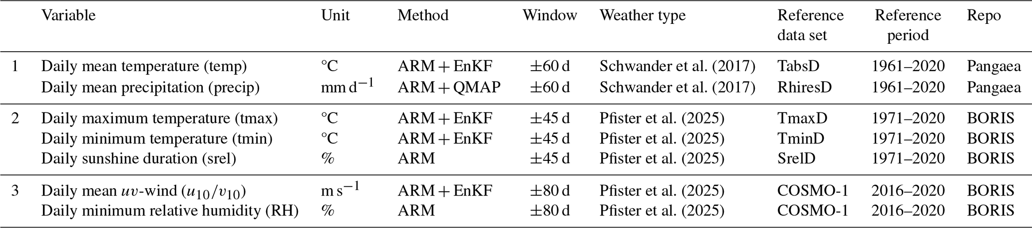
All reconstructed variables, including their methods, reference period, and reference data sets, are listed in Table 1. Note that additional indices calculated from the meteorological variables have been presented in Imfeld et al. (2024a) and are not listed.

Schwander et al. (2017)Schwander et al. (2017)Pfister et al. (2025)Pfister et al. (2025)Pfister et al. (2025)Pfister et al. (2025)Pfister et al. (2025)

Table 1 Summary of reconstructed variables. The table includes variables described in Imfeld et al. (2023) and in this article grouped by the reference periods 1961–2020 (1), 1971–2020 (2), and 2016–2020 (3). The last column indicates the repositories where the data are stored, Pangaea (Imfeld et al., 2022a) and BORIS Portal (Imfeld and Brönnimann, 2025). ARM refers to the Analogue Resampling Method, EnKF to Ensemble Kalman Fitting, and QMAP to quantile mapping. Window refers to the window size used for the analogue selection.

3.3 Data assimilation for maximum and minimum temperature

For improving the maximum and minimum temperature fields, we used an ensemble Kalman Fitting (EnKF) approach. Ensemble Kalman fitting is an offline data assimilation approach, where the analysis is not passed to the next time step, i.e., every time step is handled individually (Bhend et al., 2012; Valler et al., 2022). Data assimilation tries to find an optimal representation of the true atmospheric state between the best guess of an atmospheric field (our analogue field) and the observations by minimizing a cost function (Franke et al., 2017). In the case of normally distributed errors, this cost function can be minimized with a Kalman filter. The best estimate of a true atmospheric state, referred to as the analysis x^a, is given by Eq. (1):

$$\begin{array}{}\text{(1)}& {\mathit{x}}^{\mathrm{a}}={\mathit{x}}^{\mathrm{b}}+{\mathbf{P}}^{\mathrm{b}}{\mathbf{H}}^T({\mathbf{HP}}^{\mathrm{b}}{\mathbf{H}}^T+\mathbf{R}{)}^{-\mathrm{1}}(\mathit{y}-\mathbf{H}{\mathit{x}}^{\mathrm{b}})\end{array}$$

where x^b refers to the best estimate (the resampled analogue fields), P^b is the model error covariance matrix, H extracts the observations from the model space, and R is the observation error covariance matrix. The second part on the right-hand side of the Eq. (1) P^bH^T(HP^bH^T+R) is referred to as the Kalman gain K.

To account for a bias in the covariance analysis, we used the ensemble square root filter as proposed by Whitaker and Hamill (2002) and updated the ensemble mean and the anomaly from the ensemble mean individually, yielding two separate equations, Eqs. (3) and (4).

$$\begin{array}{}\text{(2)}& {\displaystyle }{\stackrel{\mathrm{‾}}{\mathit{x}}}^{\mathrm{a}}={\stackrel{\mathrm{‾}}{\mathit{x}}}^{\mathrm{b}}+\mathbf{K}(\stackrel{\mathrm{‾}}{\mathit{y}}-\mathbf{H}{\stackrel{\mathrm{‾}}{\mathit{x}}}^{\mathrm{b}})\text{(3)}& {\displaystyle }{{\mathit{x}}^{\prime }}^a={{\mathit{x}}^{\prime }}^b+\stackrel{\mathrm{̃}}{\mathbf{K}}({\mathit{y}}^{\prime }-\mathbf{H}{{\mathit{x}}^{\prime }}^b)\mathrm{with}:{\mathit{y}}^{\prime }=\mathrm{0}\end{array}$$

The Kalman gain for the mean K and anomaly $\stackrel{\mathrm{̃}}{\mathbf{K}}$ were then calculated as follows.

$$\begin{array}{}\text{(4)}& {\displaystyle }\mathbf{K}={\mathbf{P}}^{\mathrm{b}}{\mathbf{H}}^T({\mathbf{HP}}^{\mathrm{b}}{\mathbf{H}}^T+\mathbf{R}{)}^{-\mathrm{1}}\text{(5)}& {\displaystyle }\begin{array}{rl}\stackrel{\mathrm{̃}}{\mathbf{K}}& ={\mathbf{P}}^{\mathrm{b}}{\mathbf{H}}^T\left(\right({\sqrt{{\mathbf{HP}}^{\mathrm{b}}{\mathbf{H}}^T+\mathbf{R})}}^{-\mathrm{1}}{)}^T\\ & \times (\sqrt{{\mathbf{HP}}^{\mathrm{b}}{\mathbf{H}}^T+\mathbf{R}}+\sqrt{\mathbf{R}}{)}^{-\mathrm{1}}\end{array}\end{array}$$

We did not use a localization of the background error covariance matrix P^b because this did not change the results in Imfeld et al. (2023). For the minimum and maximum temperature assimilation, the covariance matrix P^b was calculated based on the 50 best analogue days for each target day, as it has been done in Imfeld et al. (2023). For the period from 1763 to 1864, we only had daily mean temperature observations and could not assimilate them directly into the maximum and minimum fields, but we increased the state vector by adding the analog days of the respective temperature observations. In the assimilation process, the difference between the target day and the analogue day was calculated, and therefore, no bias correction was needed. For the period after 1864, we additionally used daily maximum and minimum values in the assimilation process. Maximum and minimum temperature observations were assimilated directly into the field after correcting for their monthly bias, calculated by comparing the observations with the closest grid cell in the reference period between 1971 and 2020. The assimilation was performed on anomalies, and the climatology, corrected by a climate offset (Sect. 3.1), was added at the end of the assimilation procedure.

3.4 Data assimilation for wind fields

The data assimilation for the resampled u- and v-wind fields, largely followed the approach described for the temperature variables. We assimilated all available observations except for precipitation using an ensemble Kalman Fitting (EnKF) as described in Eqs. (1) to 5.

However, because of the extremely small analogue pool in the reference period from 2016 to 2020, we could not calculate a covariance matrix based on the ensemble members from the analogue resampling. For some of the reconstructed days, as few as 20 analogue days were available, after the restrictions on weather types and seasons with a window size of ±80 d (see Sect. 3). Therefore, we tested different approaches to obtain an adequate representation of the background error covariance matrix, including (a) using only the available members, calculating constant covariance matrices for (b) each day of the year, (c) based on the weather type classification, and (d) using a blending of a fixed climatological covariance matrix (P^clim) and the covariance matrix of the target day based on the available members (P^b) as proposed in (Valler et al., 2024). Evaluations showed that using a blended covariance matrix led to the best results, though only by a small margin (Fig. A2). The background error covariance matrix for this blending was defined as:

$$\begin{array}{}\text{(6)}& {\mathbf{P}}^{\mathrm{blend}}=\mathrm{0.5}{\mathbf{P}}^{\mathrm{b}}+\mathrm{0.5}{\mathbf{P}}^{\mathrm{clim}}\end{array}$$

P^blend was calculated using equally distributed weights of 0.5. Tests with different weights led to worse results, but no thorough testing has been performed. Whereas P^b stems from the analogue days' ensemble considering the 20 best analogue days, P^clim was calculated based on the weather type classification by randomly sampling 122 d from the same weather type (122 is the lowest number of occurrences of one weather type in 2016–2020). Due to the small sample size, we did not consider the seasons when calculating P^clim.

3.5 Evaluation of reconstructed variables

The newly generated fields are evaluated based on three approaches, (1) a cross-validation in the reference period with the original data set, (2) comparisons to historical observations, (3) and an evaluation of the consistency between the different variables.

The cross-validation was conducted by reconstructing all fields in the reference period, excluding 10 d around the target day for the ARM and the EnKF approach. We evaluated the daily data grouped into the four seasons and based on different metrics. The cross-validation was performed for each variable in their reference period as shown in Table 1, i.e., the amount of reference data used in the cross-validation differs. In addition, the cross-validation was conducted for each variable based on the different network setups as shown in Fig. 1, because the availability of observations changes largely throughout the years. In Imfeld et al. (2023), we evaluated the reconstruction approach for five different network setups. Here, we only showed the evaluation for a setup corresponding to the station availability very early during our reconstruction period (corresponding to the year 1767, lowest amount of observations), for a network around 1819, and for the network in 1934 (Fig. 1b–e). These networks are referred to as NW 1, 3, and 5 subsequently in accordance with the naming in Imfeld et al. (2023).

As for application purposes, wind speed and wind direction are more often used than the u- and v-wind components, we evaluated these variables. For wind speed, we calculated Pearson's correlation, a normalized root mean square error by dividing the root mean square error by the standard deviation of the observations (COSMO-1 wind speed), the mean squared error skill score (MSESS), and the mean bias. The MSESS is calculated using climatological mean values as a comparison. An MSESS for 1 indicates a perfect reconstruction, for an MSESS of zero, the skill of the reconstruction and climatology are equal, and for values below zero, the climatology outperforms the reconstruction (Jolliffe and Stephenson, 2012). For wind direction, we calculated the mean absolute error (MAE) based on degree values. For minimum and maximum temperature, relative humidity, and relative sunshine duration, we calculated the Pearson Correlation, the root mean square error (RMSE), the mean squared error skill score (MSESS), and the mean bias for each season. For the temperature variables, the evaluation was performed on anomalies with removed seasonality. For the wind speed and temperature reconstructions, we further evaluated how well the extreme values were reconstructed by calculating for each grid cell the mean bias and RMSE for percentiles calculated based on the original data set.

Secondly, for the variables of wind speed and daily maximum and minimum temperature, we compared the reconstructed fields to independent station observations, shown in Fig. 1 (see asterisks in b and c), matching each observation with its closest grid cell. Given Switzerland’s complex topography, elevation differences between the 1 km grid cells and station locations can be substantial, leading to significant discrepancies depending on the variable. This must be considered when evaluating against station observations.

Thirdly, we evaluated the consistency between the different reconstructed variables since they are based on different methodologies and analogue pools. For mean, maximum, and minimum temperature, we tested whether the relation $t_{\min }<t_{\mathrm{mean}}<t_{\max }$ holds. Further, we evaluated the consistency between the variables by looking at two case studies and by comparing their multivariate distributions. We chose two case studies that show a particular behaviour with respect to our reconstructed variables, namely a fog and a Foehn event. During a fog event, high values of relative humidity and low values of sunshine duration are expected, as well as low variability between tmin, tmax, and tmean in the Swiss Plateau. Depending on the height of the fog layer, furthermore, an inversion with higher temperature above the fog (and therefore at higher elevations) can be present compared to the Swiss Plateau. We considered a cross-section from the Jura (46.97° N, 6.45° E), through the Swiss Plateau to the Pre-Alps (46.62° N, 7.31° E) to evaluate this meteorological situation. This cross-section is close to the meteorological station of Payerne, for which we used a time series of fog days to find days of interest. Furthermore, we considered a Foehn event (Würsch and Sprenger, 2015) in Meiringen. A Foehn event creates higher temperatures, stronger wind speeds, lower relative humidity, and usually higher sunshine durations in Meiringen, whereas it usually leads to higher relative humidity and lower sunshine duration on the opposite side of the mountain chain. This cross-section runs from Meiringen (46.73° N, 8.20° E) to Bellinzona (46.19° N, 9.02° E) in southern Switzerland. We used a time series of the Foehn index calculated for Meiringen to define a Foehn day at this location (MeteoSwiss, 2008).

Furthermore, we compared the distributions of the different variables to their reference data for three groups, (1) the COSMO-1 variables with wind speed, relative humidity and daily mean temperature, (2) the group of minimum, maximum, and daily mean temperature, and (3) for the variables of maximum temperature and rel. sunshine duration. Distributional differences were quantified using the energy distance (Rizzo and Székely, 2016; Cannon, 2018), a metric that measures the statistical discrepancy between two multivariate distributions, which is equal to zero if and only if the distributions are identical. Energy distance was chosen because it provides a simple, non-parametric comparison of multivariate distributions. The metric was computed independently for each grid cell using subsampled daily data from 2016–2020. This period was selected because it is fully covered by all data sets used as reference. Before calculation, seasonality was removed from the temperature data, and all variables were normalized.

3.6 Canadian Forest Fire Weather Index

Using the reconstructed meteorological fields, we calculated the Canadian Forest Fire Weather Index (FWI), a widely used metric for fire danger studies worldwide (e.g., Van Wagner, 1987; Wotton et al., 2009; Vitolo et al., 2020). The FWI system comprises five sub-indices derived from the meteorological variables temperature, relative humidity, precipitation, and wind speed (e.g., Van Wagner, 1987), which build the final fire weather index (FWI). These sub-indices are the Drought Code (DC), the Drought Moisture Code (DMC), the Buildup Index (BUI), the Fine Fuel Moisture Code (FFMC), and the Initial Spread Index (ISI). The DMC, DC, and FFMC reflect varying levels of dryness at different depths of the soil and litter layers and over different timescales. The BUI combines the effects of DMC and DC, while the ISI integrates FFMC with wind speed to indicate the potential for fire spread. All sub-indices are open-ended, except for the FFMC, which ranges between 0 and 101, where 101 indicates that the fine fuel is easily ignitable. Based on the FWI, fire danger classes can be determined that are representative of their geographic region (see Kudláčková et al., 2024 for a global summary of danger classes). Originally, the FWI was calculated using instantaneous values at noon local time and 24 h precipitation accumulation (Van Wagner, 1987). However, our reconstructed data is only available at a daily resolution. Studies based on model simulations suggest that relative humidity at noon can be substituted with daily minimum relative humidity (e.g., Quilcaille et al., 2023). At the station level, we saw that using daily maximum temperature and daily minimum relative humidity produces FWI values comparable to those derived from noon observations (Fig. A1). Consequently, our calculations of the fire weather indices are based on maximum temperature and minimum daily humidity.

4 Results

4.1 Wind fields

The cross-validation results for wind speed and direction reveal the best performance in winter and the weakest in summer (Figs. 2 and 3a–d). For NW 3, the Pearson correlation ranges between −0.07 and 0.9 in winter and −0.08 and 0.83 in summer (considering all grid cells), with lower values especially in the mountains and Foehn valleys. The normalized RMSE lies between 0.44 and 1.60 m s⁻¹ in winter and 0.58 and 1.50 m s⁻¹ in summer, while the MSESS across all seasons averages above 0.6, indicating that the reconstructed wind fields outperform climatological values. Across all seasons, the mean bias is slightly negative with values as low as −0.92 m s⁻¹, except for the Swiss Plateau, where slightly positive mean biases are seen (only up to 0.45 m s⁻¹). The MAE of the wind direction shows a less homogeneous spatial picture, with locally high values, particularly in DJF and SON, reaching up to 53.88° in DJF and 40.61° in SON. However, the average remains around 6.63° in DJF and 7.88° in SON.

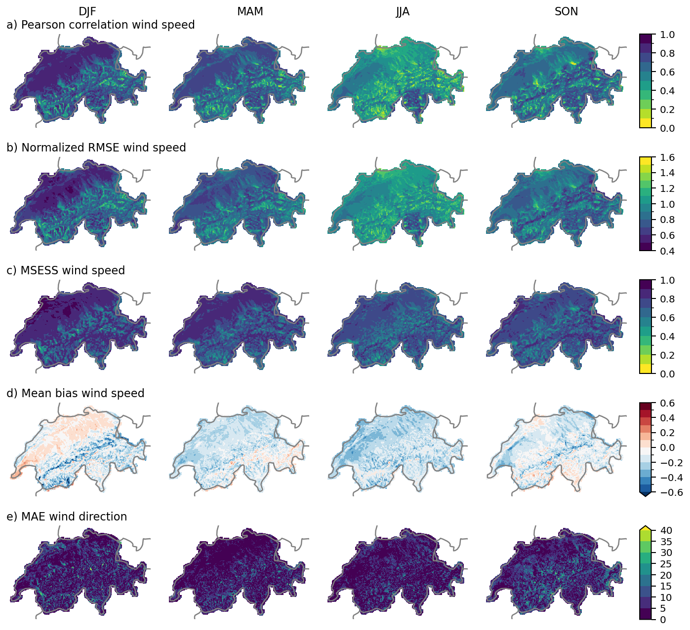
Figure 2 Cross-validation results of wind speed and wind direction for NW 3 in the reference period 2016 to 2020 and the four seasons DJF, MAM, JJA, and SON. (a) Pearson correlation, (b) normalized RMSE, (c) mean squared error skill score, (d) mean bias of wind speed, and (e) mean absolute error of wind direction. The evaluation metric for wind direction is degrees.

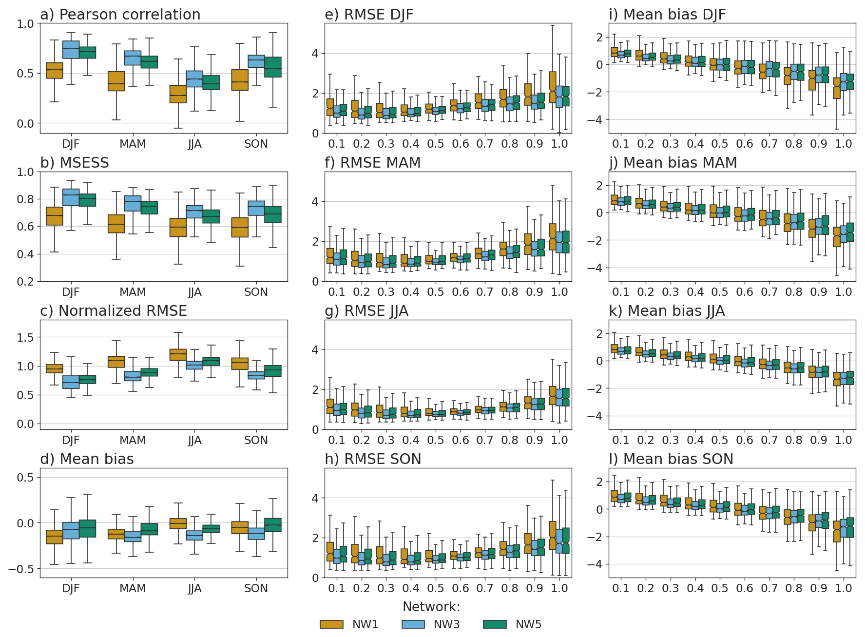
Figure 3 Cross-validation results of wind speed for the three networks (NW1, NW3, and NW5) and for the four seasons. (a) Pearson correlation coefficient, (b) MSESS, (c) normalized RMSE, and (d) mean bias of seasonal wind speed for three different networks. The second and third columns show cross-validation results calculated by deciles of the observed value for the four seasons and three networks: (e–h) RMSE of wind speed and (i–l) mean bias of wind speed. The cross-validation results are shown for successive decile bins, with the x axis indicating the upper bound of each bin. The deciles are calculated based on the reference data set separately for each grid cell.

The differences between the available network sizes are significantly smaller than those observed for the precipitation and temperature reconstructions presented in Imfeld et al. (2023). While NW 1, with only 12 observations, shows considerably lower skills in all four metrics, the results for NW 3 and NW 5 are very similar (Fig. 3a–d). NW 3 delivers the best average results across the grid for the Pearson correlation coefficient and MSESS, but also exhibits the largest (though negative) average mean bias for spring, summer, and autumn. These findings suggest that adding more stations beyond a certain threshold does not further enhance reconstruction quality. For networks with more than 43 available records (NW 5), we tested various setups for the analogue resampling method (ARM) and data assimilation (Fig. A2). Selecting a specific subset of stations instead of all available stations increased the Pearson correlation by up to 0.1.

As expected, all seasons exhibit the largest RMSE values for the highest percentiles of wind speed, with NW 1 consistently producing the largest errors (Fig. 3e–h). For the lower half of the percentiles, the RMSE remains relatively constant, though the spread of errors increases again for the smallest percentiles. This pattern suggests that very low wind speeds are more prone to overestimation, as reflected in the mean bias calculated by percentile (Fig. 3i–l). Across all seasons, the mean biases reveal an overestimation of low wind speeds and an underestimation of high wind speeds. This is likely due to the limited size of the analogue pool used for wind reconstruction, which affects the accurate representation of high wind speeds.

We further compared the wind reconstructions to independent measurements from the Saentis, Segl Maria, and Neuchâtel stations, with observations starting in 1882, 1864, and 1901, respectively (Fig. 4). Pearson correlation coefficients between the reconstructions and observations for the full overlapping period are 0.46 (Saentis), 0.25 (Segl Maria), and 0.53 (Neuchâtel), indicating rather low agreement, as also seen in the comparison of time series and the scatterplots in Fig. 4a–f. The highest correlations with station measurements are found for Geneva, with a Pearson correlation coefficient of 0.56, which, however, only started measuring in 1958. Especially in the late 19th and early 20th centuries, wind speed measurements had a lower measurement resolution (see lines of measurements at certain accuracies in Fig. 4d, e, f) and measurement problems occurred, such as freezing of the anemometer on the Saentis at 2501 m a.s.l. (Hupfer, 2019). Also, the wind measurements have not been controlled for quality and homogeneity, which can both affect the comparison with the reconstruction. Furthermore, a 1 km resolution grid cannot fully capture the highly localized effects of wind in complex terrain, which further reduces agreement between the reconstruction and observations, as shown by Kruyt et al. (2018) for the COSMO-1 model.

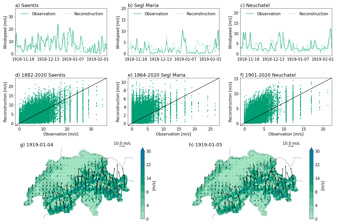
Figure 4 Comparison of reconstructed wind fields to independent observations. (a–c) Time series for the location of Saentis, Segl Maria, and Neuchâtel compared to observations during a strong Foehn event from 4 to 5 January 1919. (d–f) Scatterplots of all available wind speed measurements for the three stations. (g) and (h) 10 m wind speed (colour) and wind arrows for the strong Foehn event on 4 and 5 January 1919. The locations of the stations are shown in Fig. 1.

From 4 to 5 January 1919, a strong Foehn storm occurred due to a record-low pressure north of the Alps, causing substantial damage across Switzerland. This event has been classified as one of the eight extreme storms in Switzerland since 1856 (Stucki et al., 2014). For the time series, Segl Maria and Saentis, the reconstruction shows peak values around 4 and 5 January, but not for the station in Neuchâtel, which is not prone to strong Foehn winds (Fig. 4a–c). The strong Foehn winds are very pronounced throughout the Alps as seen in the maps of Switzerland (Fig. 4g and h). However, this remains a rather qualitative assessment, and we cannot determine how realistically, for example, the spatial pattern of the wind field is reconstructed.

4.2 Maximum and minimum temperature

The cross-validation results for maximum and minimum temperatures are presented for NW 5 shown in Fig. 1b. For this network, we also incorporated the available maximum and minimum temperature observations. For comparison, the spatial analyses for NW 3, when no maximum and minimum temperature observations were available, are shown in Fig. A3.

For maximum temperature, cross-validation results show very high Pearson correlation coefficients across all seasons, with higher values especially north of the Alps, ranging between 0.77 and 0.99 for individual grid cells (Fig. 5a). In contrast, minimum temperature exhibits a more fragmented pattern, with the highest Pearson correlation coefficients concentrated around northern Switzerland and generally lower values south of the main Alpine ridge (Fig. 5d). For individual grid cells, the Pearson correlation coefficients, however, still remain between 0.66 and 0.98. The RMSE shows very similar values between the two variables, with on average even slightly lower errors for minimum temperature (1.29 °C) than for maximum temperature (1.33 °C) and generally lower errors in the Swiss Plateau, where also on average more observations are available. Both maximum and minimum temperatures exhibit relatively few seasonal differences. In winter, the RMSE for minimum temperature reveals a distinct pattern, with the highest errors occurring in the region of La Brévine – one of the coldest areas in Switzerland due to topographic and radiative effects. Additionally, RMSE values are larger in the higher elevations of the Canton of Ticino in southern Switzerland, likely due to the lack of observations at higher altitudes. Overall, biases range from −0.2 to +0.2 °C for maximum and minimum temperatures. The cross-validation for maximum temperature shows overall slightly better results than for minimum temperature, despite the availability of fewer observations for assimilation (10 series for maximum temperature and 14 for minimum temperature). This might be because maximum temperature values are spatially more homogeneous and less influenced by local effects, such as lake effects and cold air pools.

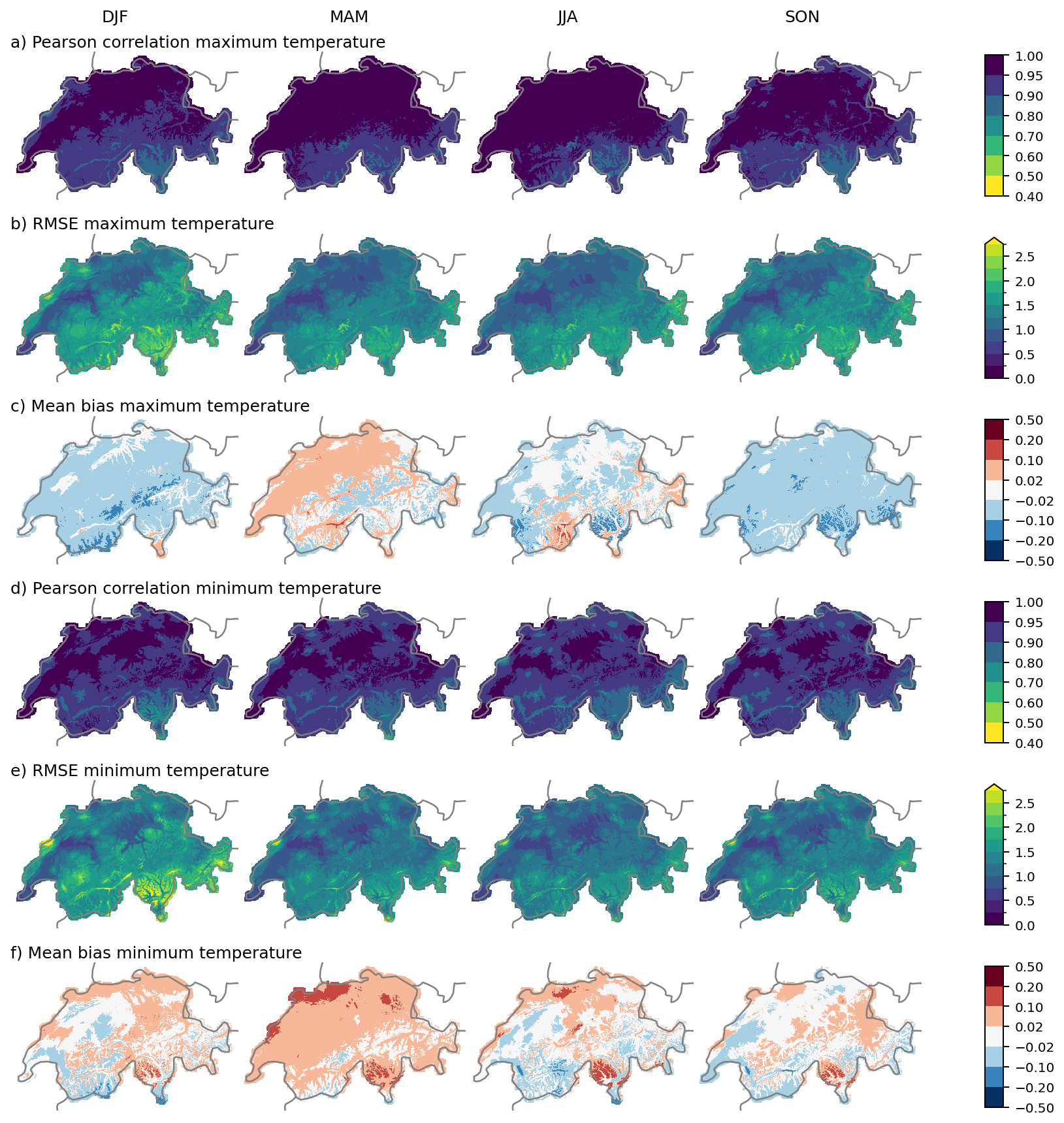
Figure 5 Cross-validation of maximum and minimum temperature for NW 5 in the period 1971 to 2020 and the four seasons DJF, MAM, JJA, and SON. (a) Pearson correlation coefficient, (b) RMSE, (c) mean bias of maximum temperature, and (d) Pearson correlation coefficient, (e) RMSE, (f) mean bias of minimum temperature. All metrics are calculated based on temperature anomalies with removed seasonality.

The different networks show considerable differences, with the periods after 1864, when maximum and minimum temperatures can be assimilated, outperforming the earlier periods (Fig. 6a–d). For example, the network representing the period around 1819 (NW 3) has a mean Pearson correlation coefficient between 0.88 and 0.91, depending on the season for maximum temperature and between 0.81 and 0.86 for minimum temperature (see also Fig. A3). In contrast, NW 1 shows Pearson correlation coefficients of only between 0.75 and 0.88 on average per season for maximum temperature and between 0.73 and 0.76 on average for minimum temperature, which is considerably lower than NW 5. Furthermore, both the minimum and maximum temperature of NW 1 have with an average RMSE of up to 3.1 °C much larger errors in winter compared to the other seasons and networks.

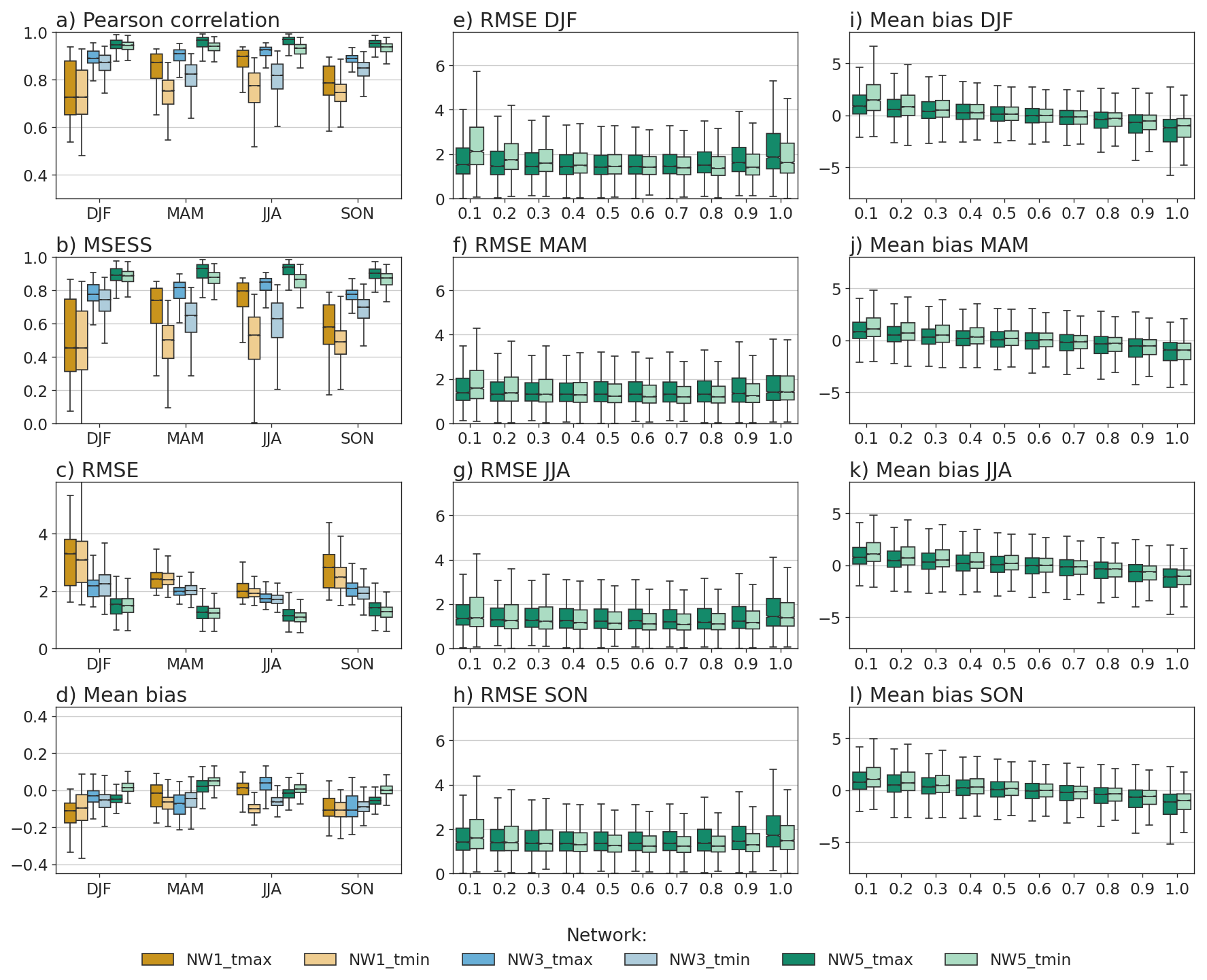
Figure 6 Cross-validation results of maximum and minimum temperature for the three different networks (NW1, NW3, and NW5) and the four seasons. (a) Pearson correlation, (b) MSESS, (c) RMSE, and (d) mean bias of maximum and minimum temperature. The second and third columns show cross-validation results calculated by deciles of the observed value for the four seasons and three networks: (e–h) RMSE of maximum and minimum temperature, and (i–l) mean bias of maximum and minimum temperature. The cross-validation results are shown for successive decile bins, with the x axis indicating the upper bound of each bin. The deciles are calculated based on the reference data set separately for each grid cell.

The other metrics also show lower performance when no maximum or minimum temperature could be assimilated. The earlier networks exhibit poorer results in summer and spring for minimum temperature, showing also a large spread in the metrics. The mean biases are larger for the earlier networks, but remain within −0.22 to +0.13 °C for NW 3.

The percentile evaluation has only been performed for NW 5. It shows that the reconstruction has the largest RMSE for maximum temperature when estimating the highest temperature percentiles and for minimum temperature when estimating the lowest temperature percentiles (Fig. 6e–h). For the average percentiles, errors for minimum and maximum temperatures are relatively similar, though they are consistently slightly lower and exhibit less spread for maximum temperature. The mean bias evaluation indicates that the lowest temperature values are consistently overestimated in the reconstruction, while the highest values are consistently underestimated across all seasons, with the largest biases occurring in winter (Fig. 6i–l).

It is furthermore relevant to consider whether the daily mean temperature always lies between the daily minimum and maximum temperature since we did not explicitly control for this in the reconstruction method. Our analogue fields for maximum and minimum temperature already incorporate this, however, the daily mean temperature is based on different analogue days. Controlling the data sets for such inconsistencies shows that in the period from 1763 to 1863, for on average 2.5 % of the grid cells per year maximum temperature is lower than the daily mean temperature. The year 1812 has a record high with 4.2 % of the grid cells having lower maximum temperature values than daily mean temperature values. This high percentage stems from some individual days where the analogue days differed considerably. For minimum temperature, on average 1.7 % of the grid cells per year show a higher value than the daily mean temperature. The largest fraction of days and grid cells above the daily mean temperature occurred in 1766, with 3.1 %. As soon as maximum and minimum temperatures were assimilated (starting in 1864), the percentage of too high/low values is reduced to on average 1.7 % for maximum temperature and 0.8 % for minimum temperature. However, the inconsistencies have a clear annual cycle, with most of the under- or overestimations happening in the winter season.

We further compared the reconstructions to measurements from Château-d'Oex and Segl Maria (see Fig. 1b for locations). Both locations are situated at the bottom of valleys in mountainous areas. While we used daily mean temperature during the assimilation, we did not include the maximum and minimum measurements of these stations in the reconstruction due to the short or incomplete nature of these series. For all four time series, the closest grid cell of the reconstruction agrees well with the observation (Fig. 7). For Château-d'Oex, the Pearson correlation coefficient is as high as 0.92 for maximum temperature and 0.89 for minimum temperature in the period 1931–2020. For Segl Maria, the Pearson correlation coefficient is 0.88 for maximum temperature and 0.84 for minimum temperature in the period 1869–1970. RMSE for minimum and maximum temperature at both locations are between 1.82 and 2.15 °C and mean biases are between −0.07 and +0.03 °C, all indicating that the reconstructions correspond well to the observations.

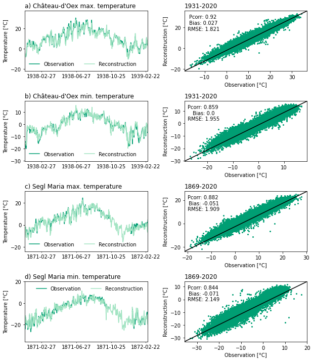
Figure 7 Comparison of reconstructed maximum and minimum temperature fields to independent observations. (a, b) Time series for the location of Château-d'Oex compared to observations during one year of measurements and scatter plot for the entire period of measurements from 1931 to 2020. (c, d) Time series for the location of Segl Maria compared to observations during one year of measurements and scatter plot for the entire period of measurements from 1869 to 2020 (with gaps). The time series have not been used for the reconstruction, but they have been used in creating the original gridded data set. The location of the independent stations is shown in Fig. 1.

4.3 Relative sunshine duration

The relative sunshine duration reconstruction is derived from the analogue days used for maximum and minimum temperature reconstruction without additional post-processing. This analogue pool spans 50 years (1971–2020), providing a sufficiently large data set. Cross-validation results show a strong dependence on the observational network, with generally better performance for networks with a higher number of observations (Fig. 8a–c). Pearson correlation coefficients across all networks and seasons average above 0.4, though notable seasonal differences exist, with the best results in summer, followed by spring. The MSESS values range on average between −0.21 in DJF (NW1) and 0.48 in JJA (NW5). For NW1, the reconstruction of the relative sunshine duration is, therefore, largely outperformed by the climatology. For NW 5, the network with the most observations, the reconstruction on average outperforms climatology as a reference for all seasons. However, it should be considered that for applications such as impact modeling, climatology may not be a suitable comparison because a climatological forecast lacks variance. The expected MSESS for predictions with the correct variance but no correlation is −1. The RMSE values are all very high, with average values between 20 %–40 %. Nevertheless, the mean biases are rather small, indicating a correct distribution as expected. The mean biases do not show a clear pattern based on seasons, but on networks. Networks 1 and 3 tend to overestimate the relative sunshine duration in all seasons, while NW 5 tends to underestimate sunshine duration in winter. Note that for NW 1 and 3, all available data was used, whereas for NW 5, only temperature data was used because this led to better results for the maximum and minimum temperature reconstruction.

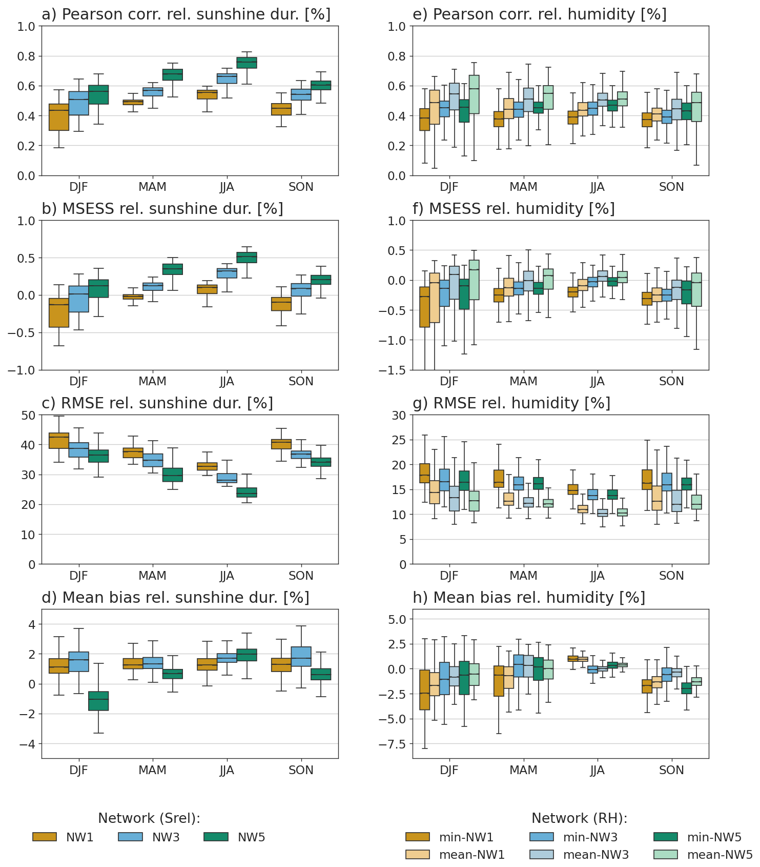
Figure 8 Cross-validation results for relative sunshine duration and relative humidity across the different networks and seasons. (a) Pearson correlation coefficients, (b) MSESS, (c) normalized RMSE, and (d) mean bias of seasonal relative sunshine duration for the three different networks. (e) Pearson correlation coefficients, (f) MSESS, (g) RMSE, and (h) mean bias for daily minimum and daily mean humidity considering the three networks. Relative sunshine duration is evaluated in the reference period from 1971 to 2020, and relative humidity is evaluated from 2016 to 2020.

4.4 Relative humidity

The relative humidity fields have been extracted from the COSMO-1 model output for the same analogue days used for the wind fields. Since we focused on reconstructing wind fields rather than relative humidity, we did not optimise the analogue selection for relative humidity. Accordingly, cross-validation results for minimum and daily mean relative humidity indicate limited skills, with daily mean values consistently performing better than minimum values (Fig. 8d–f). Pearson correlation coefficients range, on average, from 0.39 to 0.59, depending on the season and the network. The MSESS for daily mean and minimum relative humidity ranges from −0.31 to 0.06, indicating that the reconstruction performs as good as the climatology or worse. These are not very convincing results, however, we optimised the analogue days for the wind reconstruction. Excluding, for example, many precipitation observations from the calculation of the analogue days could have deteriorated the relative humidity reconstruction. It should be considered that an advantage of our reconstructed variables is that they are physically largely consistent with each other as they stem from similar analogue days. Moreover, in comparison to using climatological mean values, our reconstruction captures the variance. The RMSE averages between 10 %–13 % for mean daily relative humidity and 14 %–18 % for minimum relative humidity. However, biases remain small, reaching at most −3 % on average. A small bias is expected because the values are sampled from the same distribution based on season and weather type. Both, the daily mean and minimum relative humidity are underestimated in all seasons, except for JJA. These relatively low scores are expected, as no additional postprocessing was applied to the relative humidity fields, and the analogue pool for the selection of fields was very small. Nonetheless, we consider it important to provide these fields, since they are necessary for certain types of studies.

5 Consistency and uncertainty of the reconstructed fields

5.1 Consistency analyses

Because of differences in analogue pools and reference data, variables may show reduced internal consistency. The example of fog on the Swiss Plateau shows that the temperature variables agree well in their spatial behavior for this fog day on 23 January 2017. Higher values occur in the Pre-Alps, while lower values are observed over the Swiss Plateau. Overall, the expected relationship t_min  < t_mean < t_max holds across the entire cross-section (Fig. 9a).

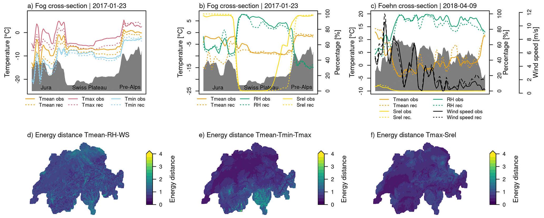
Figure 9 Consistency of the different variables based on cross-section of (a–b) a fog day in the Swiss Plateau on the 23 January 2017 and (c) a Foehn day in Meiringen on 9 April 2018. The dashed lines show the reconstruction, while the solid lines show the reference data set (i.e. observations). The maps of energy distance are shown for (d) daily mean temperature, relative humidity and wind speed, (e) maximum, minimum, and daily mean temperature, and (f) maximum temperature and sunshine duration.

For relative humidity and sunshine duration, the general pattern of low sunshine duration over the Swiss Plateau and higher values in the surrounding mountain regions (Jura and Pre-Alps) is also reproduced. However, in the reconstructed data, the area of low sunshine duration extends further towards the Alps than in the reference data. This leads to stark inconsistencies between sunshine duration and temperature patterns. Similarly, relative humidity exhibits high values over the Swiss Plateau and lower values on both mountain flanks matching the pattern of the daily mean temperature (Fig. 9b).

A further illustrative case occurs during a Foehn event. Under Foehn conditions in Meiringen, wind speeds are expected to be high, while relative humidity is low and sunshine duration is high. On 9 April 2019, these variables show good agreement with each other, and also correspond well with the reference data sets, indicating that the variables are largely consistent for this event (Fig. 9c).

To examine the consistency of the variables beyond individual events, we calculated the energy distance between the distributions of the reference data sets and the reconstructions (Fig. 9d–f). Values close to zero indicate good agreement between the multivariate distributions. In this context, the metric mainly allows an assessment of spatial differences, that is, where the distributions agree well with the reference data and where they diverge.

For the combination of mean temperature, relative humidity, and wind speed (with COSMO-1 used as the reference for the three variables), several regions stand out with larger energy distance values (Fig. 9d). These include parts of the Swiss Jura, such as La Brévine, which is known for very cold conditions, as well as areas along the Rhône Valley in Valais, in Ticino, and in northern Switzerland. These locations are associated with either very cold conditions or Foehn-affected valleys.

For the group of maximum, minimum, and daily mean temperature (Fig. 9e), the energy distance is close to zero mainly in northern Switzerland, whereas higher values occur in Ticino and in some high-mountain areas. One possible explanation for this pattern is the scarcity of observations in southern Switzerland and at higher elevations. Furthermore, the comparison between Tmax and relative sunshine duration is comparatively homogeneous with no stark spatial patterns (Fig. 9f). These reconstructions are based on the same reference data pool and analogue days and therefore exhibit better mutual agreement. For several pairs of distributions, their joint density estimates are shown in Fig. A4.

To qualitatively assess the long-term consistency of the reconstructed variables, we analyzed the 258-year field mean, smoothed using a 1-year running average (Fig. 10). The wind speed reconstruction shows no substantial long-term changes. However, for a prolonged period around 1900, the field means do not exceed 2.25 m s⁻¹, suggesting a possible underestimation of wind speeds during that period. The temperature reconstructions agree very well with each other, which is not surprising since they all assimilate the same daily mean temperature data. Prominent features in the data set are, for example, the increase around the late 1940s, which is known as a warmer and drier period in the 20th century (Imfeld et al., 2022b). This same climate anomaly is also reflected in the increase of the relative sunshine duration around the late 1940s and in a slight decrease in the daily mean relative humidity values. Relative humidity shows a slight decrease in values throughout the entire period. It is not clear whether this can be attributed to the reconstruction method and is therefore an artifact; however, studies on much shorter time scales suggest a decrease in relative humidity over Europe, for example, since the 1980 (e.g. Copernicus Climate Change Service, 2022). Certain patterns, such as lower values for sunshine duration, increased values for relative humidity, and increased values for precipitation between the 1830s and 1850s seem to be consistent in the different variables, despite the different analogue days as input.

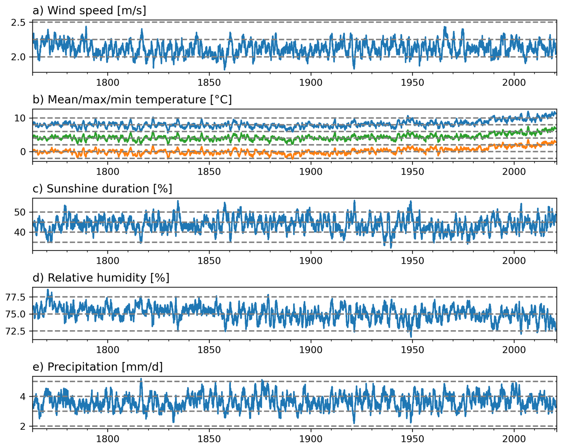
Figure 10 Long-term evolution of the reconstructed variables. (a) Daily wind speed [m s⁻¹], (b) daily mean, maximum, and minimum temperature [°C], (c) daily relative sunshine duration [%], (d) mean daily relative humidity [%], and (e) daily precipitation sums [mm d⁻¹] for comparison. The time series shows the area mean across the entire Switzerland, smoothed with a 1-year running mean.

5.2 Uncertainty

Uncertainties in the dataset primarily arise from two sources: instrumental observation errors, particularly in the early periods, and uncertainties related to the reconstruction method. Observation errors in individual time series are discussed in detail by Brugnara et al. (2022), which serves as a key reference on the types and magnitudes of errors in early instrumental records. They distinguish four main error types: reporting resolution, number of measurements, timing, and exposure. Limited reporting resolution and a small number of measurements reduce the accuracy of daily mean estimates, while inaccurate timekeeping, especially before the 19th century, complicates consistent observation times. Exposure errors arise from radiative biases, for example, due to unshielded thermometers. A fifth error related to changing measurement locations is reported in Brugnara et al. (2022) but is not relevant here, as measurements are used at their original locations. Error magnitudes, however, vary between series and also over time. For the Swiss series, the CHIMES publications Brönnimann (2020) provide additional insight into data quality and uncertainties, helping users to interpret the dataset and consider its caveats.

Additional uncertainty arises from the reconstruction method itself. Although the analogue resampling approach produces an ensemble that can, in principle, be used to estimate uncertainty, our implementation yields an ordered ensemble, where higher-ranked members are closer to the true atmospheric state than lower-ranked ones, depending on the distance metric. Nevertheless, the ensemble still provides an indication of the spread in the reconstructed variables. Figure A5 shows the ten best ensemble members for a late-summer period in 1957 for all reconstructed variables, though at different reconstruction stages. For daily mean temperature, the ensemble after data assimilation is displayed, as provided in Imfeld et al. (2024a), while for the other variables, only the analogue-based ensembles are shown. For minimum and maximum temperature, and the u- and v-wind components, the ensemble spread is expected to decrease further after assimilation. In contrast, the analogue ensembles suggest that reconstructions of relative sunshine duration and relative humidity are less robust, likely because these variables are not constrained by direct observational input during the reconstruction.

6 Historical wild fire reconstructions

The reconstructed fire weather indices enable us to study the conditions that led to historical wild fires over the past centuries, while acknowledging that early data may be subject to uncertainty. As shown by the evaluation of the individual variables, the quality of the reconstruction depends strongly on the time period chosen, which directly affects the reliability of derived indices such as the Canadian forest fire weather index.

Here, we examined three notable forest fires in Switzerland, one in August 1911, another in the summer of 1943, and a more recent fire in the winter of 2016, which allows for comparison with the COSMO-1 weather forecast model. On 20 August 1911, a forest fire broke out in the Canton of Bern, on the steep mountainous slope called the Simmenfluh (asterisks in Fig. 11 a and b) ignited by lightning from a passing storm, as stated in the newspaper “Die Berner Woche in Wort und Bild” (Werder, 1911), which was published at that time. Although the fire was extinguished within a few days, embers remained in the calcareous ground, reigniting it. The fire was only fully extinguished on the 22nd of September with the onset of heavy rainfall and led, in total, to damage of around 100 ha of burnt forest. The summer half year of 1911 was very dry and warm, as reflected in the high values of the DC (Fig. 11a). The FWI was variable across Switzerland on 19 August 1911 with high levels especially in the Swiss Plateau (Fig. 11b).

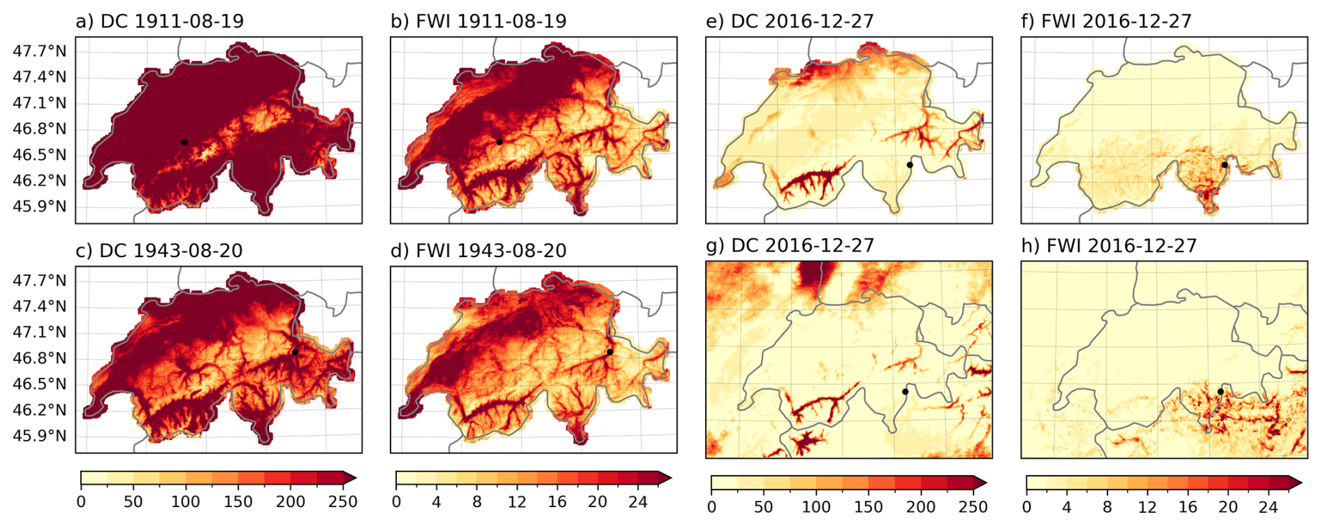
Figure 11 Drought code (DC) and fire weather index (FWI) for the three forest fires in the reconstruction. (a, b) Forest fire in Simmenfluh, 1911, (c, d) forest fire in August 1943 on the Calanda mountain slopes, (e, f) forest fire in Misox in winter 2016. (g, h) show the forest fire in Misox, but based on the COSMO-1 model. The approximate locations of the fires are shown as black dots in each panel.

Another significant fire occurred on the slopes of the Calanda massif above the city of Chur (asterisks in Fig. 11 c and d) following shooting exercises by the Swiss army on 20 August 1943. The fire grew rapidly due to the onset of Foehn winds and dry weather conditions, resulting in massive smoke plumes around the Calanda mountain (Bouchorikou, 2024; Fuchs, 2024). The fire was only fully extinguished after three days, causing significant damage to infrastructure and destroying 477 ha of forest. For this event, the DC indicated particularly high values for the valleys around Chur, but also in the Swiss Plateau and the southern valleys (see asterisks in Fig. 11c). The FWI, however, was less pronouncedly high across Switzerland, with only the Rhone Valley, the Swiss Plateau area, and the Rhine Valley showing values above 24 (Fig. 11d). The summer of 1943 was part of a series of relatively warm and dry summers in the 1940s (Imfeld et al., 2022a).

To compare the indices with those calculated from the model, we also considered two independent modern fires happening in the Moesa region (asterisks in Fig. 11e and h) in December 2016, which led to the evacuation of two houses and caused damage to around 120 ha of forest (Schildknecht, 2017; Fuchs, 2024). In contrast to the two historical fires, the DC and FWI values were considerably lower across Switzerland. Even though December 2016 has been exceptionally dry and with a very low snow-coverage (MeteoSwiss, 2017), the DC index does not show particularly high values for the Moesa region on 27 December 2016 neither in the reconstruction nor the COSMO-model (see asterisks in Fig. 11). FWI values were generally low across Switzerland, averaging 2.72 in the reconstruction. However, in the village of Mesocco, located in the Moesa region, FWI values reached up to 18.7 on 28 December 2016 in the reconstruction (Fig. 11e–h), and the spatial pattern shows good agreement between the COSMO model and the reconstruction. In fact, the warning from the Federal Office of Environment, which is responsible for disseminating forest fire warnings, indicated a severe fire danger level on 23 December (level 3), and changed it to extreme (level 4) on 28 December 2016 when the fires were already burning. December 2016 has been exceptionally dry with very low snow coverage in these areas, even though this is not seen from the DC index.

These short evaluations show that the data set seems suitable for studying certain climate impacts in the past, such as the occurrence of fire weather conditions in Switzerland.

7 Data availability

The reconstruction data set is available at https://doi.org/10.48620/87086 in the Bern Open Data Repository (BORIS) (Imfeld and Brönnimann, 2025). It extends the already available data sets for daily mean temperature and daily precipitation sum available at https://doi.org/10.5194/cp-19-703-2023 (Imfeld et al., 2022a) and described in Imfeld et al. (2023). Indices calculated from daily temperature and precipitation can be found in Imfeld et al. (2024a) and are described in Imfeld et al. (2024b). All variables and indices calculated in this article are listed in Table 1.

8 Code availability

The code is available at https://doi.org/10.5281/zenodo.19650680 (Imfeld, 2026).

9 Conclusions

This study expands high-resolution historical meteorological reconstructions by incorporating important variables, such as wind, relative humidity, sunshine duration, and maximum and minimum temperature, alongside the existing reconstructions of daily mean temperature and daily precipitation sums. Spanning the period from 1763 to 2020, the data set represents an advancement for studying historical weather patterns in Switzerland, made possible through the integration of rescued early instrumental data, the analogue resampling method, and ensemble Kalman fitting.

Cross-validation results demonstrate convincing results for the temperature and wind variables for the period after 1864, when in Switzerland a high-quality and dense observational network started to be set up. For this period, maximum and minimum temperature perform very well with Pearson correlation coefficients ranging between 0.81 and 0.91 and MSESS between 0.48 and 0.82. Wind speed also shows good correlations and MSESS values of 0.70 to 0.80 despite being derived from a very small analogue pool. Relative sunshine duration and relative humidity, however, exhibit moderate to low performance, not clearly outperforming climatological values. However, an advantage of our reconstruction is that the variables are largely physically consistent with each other since they stem from the same or similar analogue days, and that they capture variance in the data set which is not given using climatological mean values.

The validation against observational data, especially for the temperature variables, further confirms the robustness of the reconstructed fields for this period, with correlations of up to 0.92 calculated on anomalies. Before 1864, when observations were sparser and of lower quality, maximum and minimum temperatures still performed considerably well, while wind speed showed significantly worse performance, especially for the very sparse network in the 1760s. Nevertheless, the MSESS values show that most of the reconstructed fields perform better than when using a climatological value, which can be helpful for certain applications. When working with this data, the limitations and the different skills, especially for the variables of relative humidity and relative sunshine duration throughout the time periods, have to be carefully considered. New methods, such as machine learning, and updated data products, such as time series of maximum and minimum temperature reaching further back and in-depth homogenized pressure data, could help to substantially improve future versions of such weather reconstructions. Also, a lot of historical weather notes are available describing the cloud coverage of the sky. Especially for sunshine duration, they could be a variable source for evaluating the reconstruction in the past, but methods could also be explored to include such information in the reconstruction process.

Despite these limitations, the data set described here is the first attempt to provide long-term, high-resolution gridded data for several key meteorological variables. The inclusion of these additional variables enables a broader range of applications, such as calculating the Canadian Forest Fire Weather Index, which provides valuable insights into historical fire weather and fire danger, as shown by the two examples of forest fires in 1911 and 1943 in Switzerland.

Appendix A

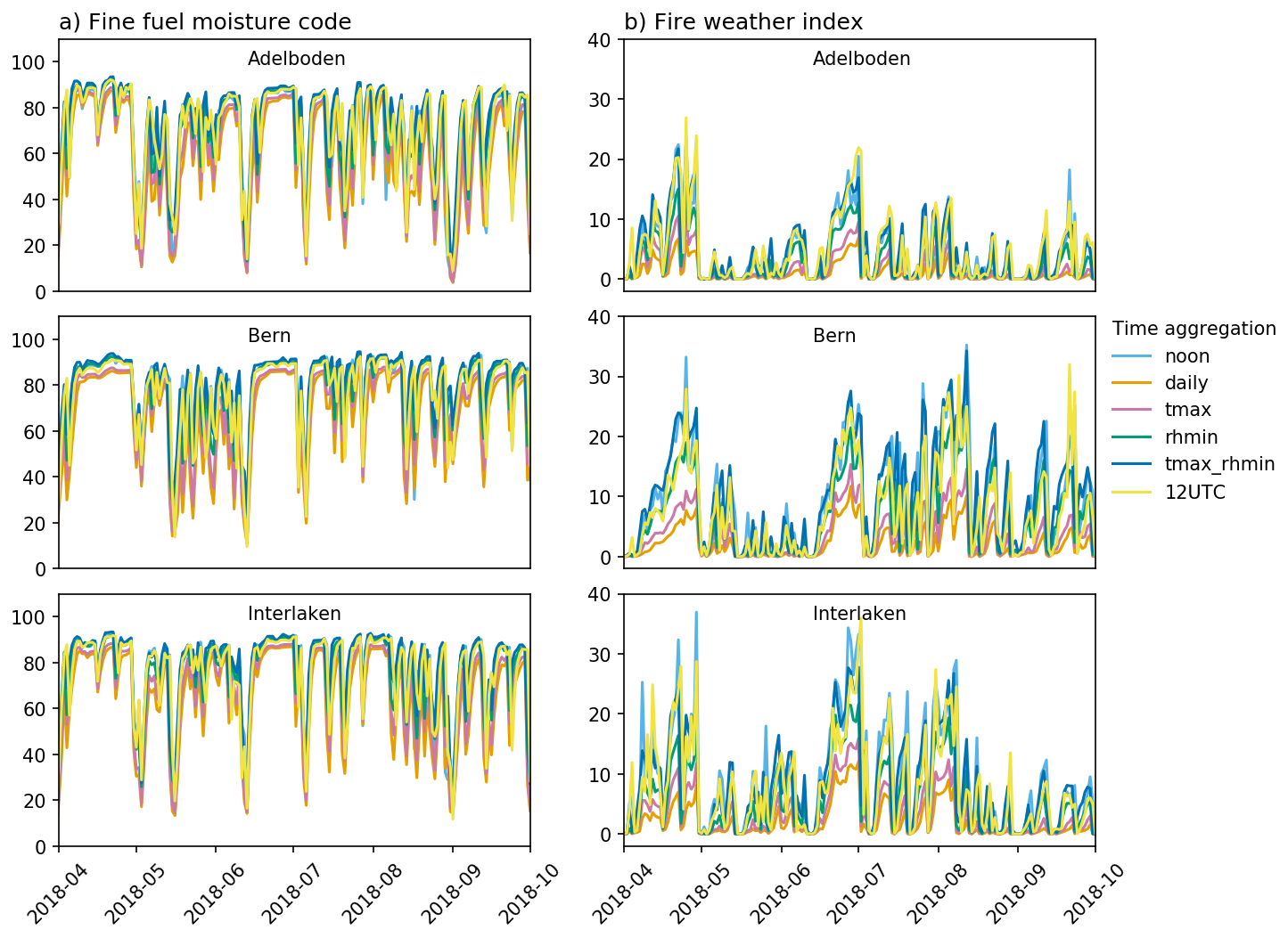
Figure A1 Comparison of FFMC and FWI calculated with different time aggregations for the weather stations in Bern, Adelboden, and Interlaken between April and August 2018. Noon refers to noon local time, daily refers to the daily mean aggregation between 00:00–24:00 for all variables except precipitation (6-6 aggregation), t_max and RH_min are maximum and minimum values between 00:00–24:00 of the respective variables. These evaluations show that using the daily maximum temperature and daily minimum relative humidity yields values similar to noon values.

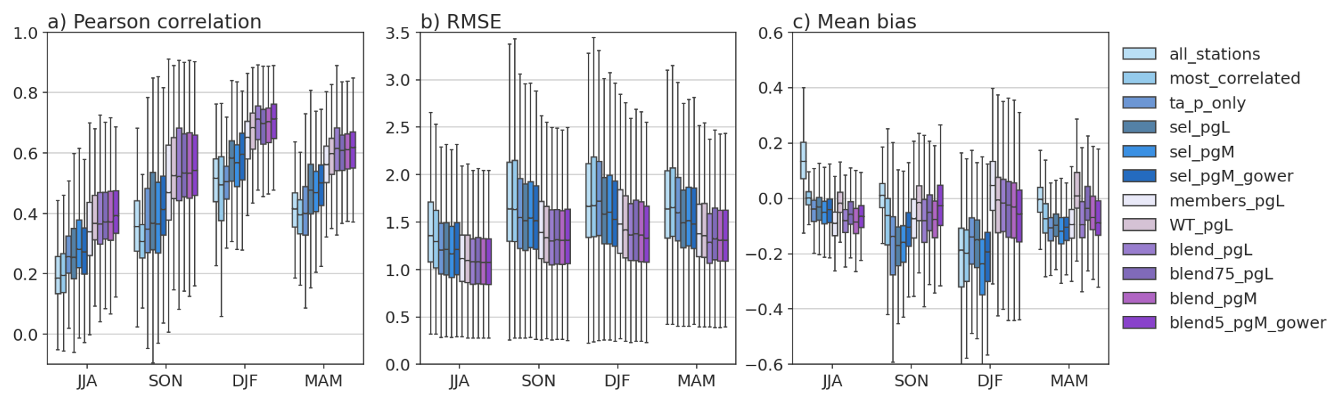
Figure A2 Comparison of evaluation results for the wind speed reconstruction depending on season. Blue colours represent evaluations for ARM only using different network set-ups, purple colours represent evaluation based on ensemble Kalman fitting, based on different calculations of the background error covariance matrix. Table A1 describes the different inputs.

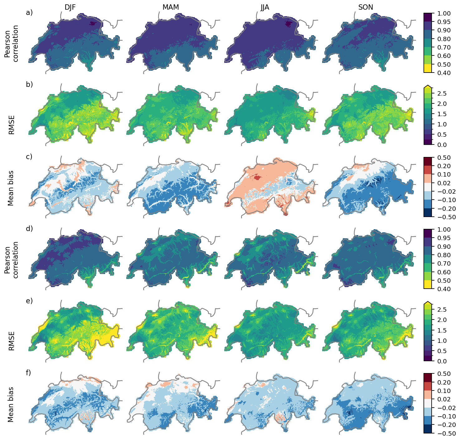
Figure A3 Cross-validation of maximum and minimum temperature in the period 1971 to 2020 for the four seasons DJF, MAM, JJA, and SON. (a) Pearson correlation coefficient, (b) RMSE, (c) mean bias of maximum temperature, and (d) Pearson correlation coefficient, (e) RMSE, (f) mean bias of minimum temperature. The maps show the cross-validation results of NW 3. All metrics are calculated based on temperature data with removed seasonality.

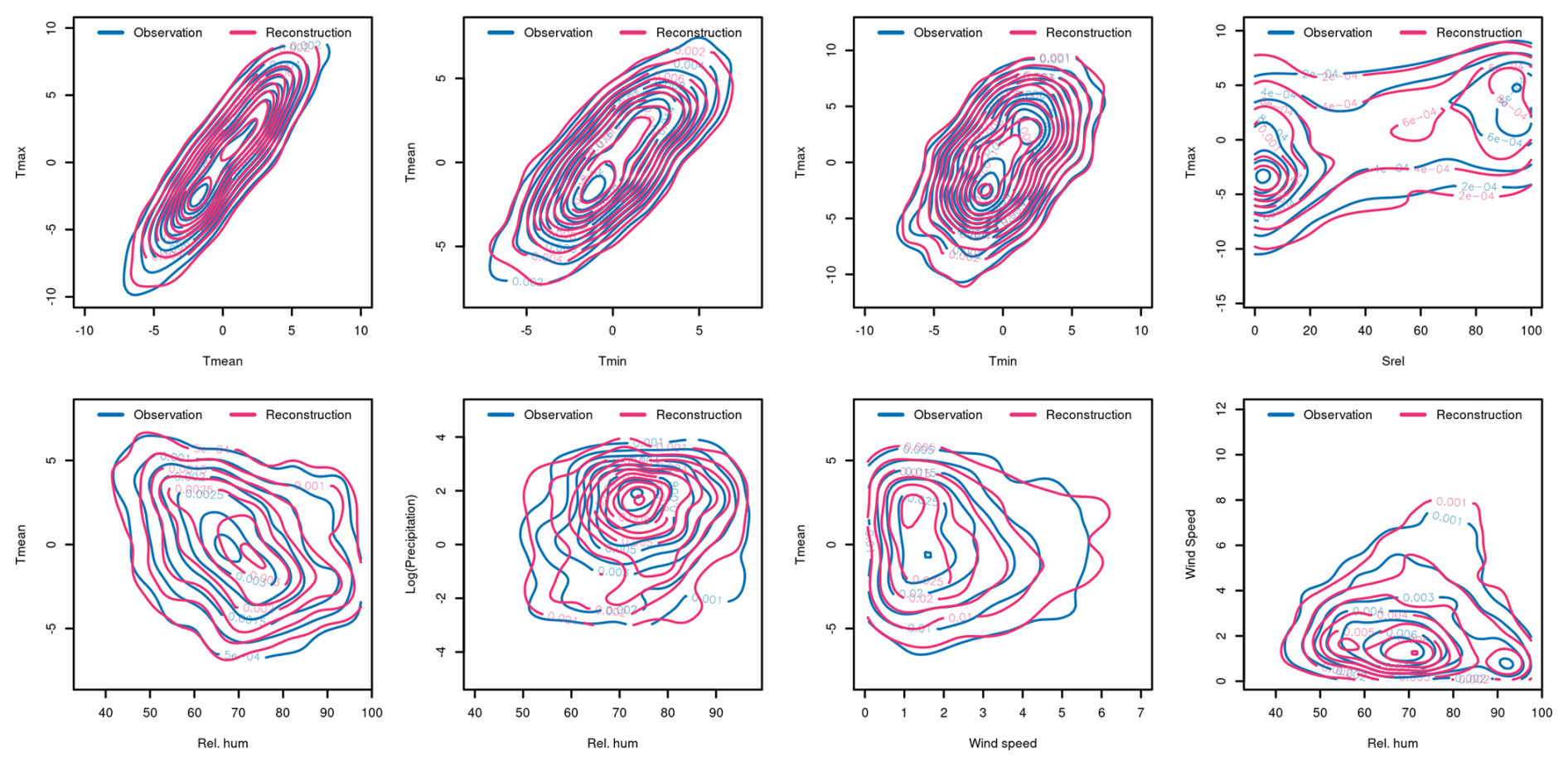
Figure A4 Density plots of pairwise variable distributions for the observed data and their reconstructions, estimated using two-dimensional kernel density for the years 2016 to 2020. For the temperature variables, we used deseasonalized data, the precipitation data was log-transformed for values > 0.05 mm. The evaluation was made for the grid cell at 2553500 E, 1183500 N (Swiss coordinate system LV95).

Table A1 Description of different reconstruction set-ups for ARM and EnKF for reconstructing uv winds for the full network as it was available after 1934. The variables are daily mean temperature (t_a), daily mean pressure (p), daily precipitation sum (rr), and daily precipitation occurrence (rr0). PH refers to the reduced covariance matrix.

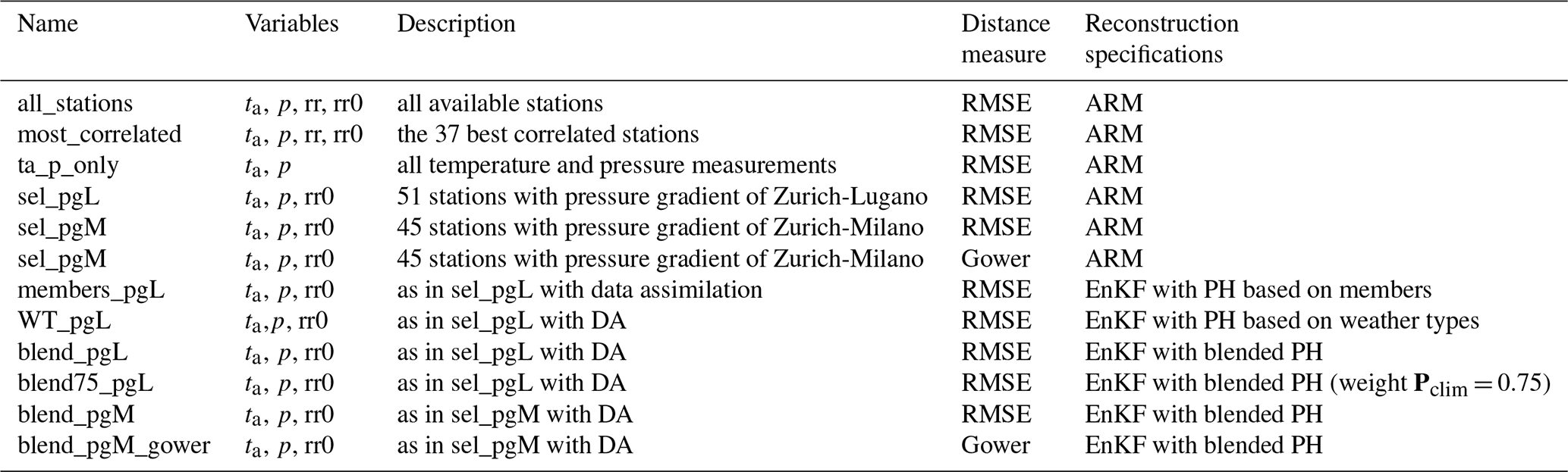
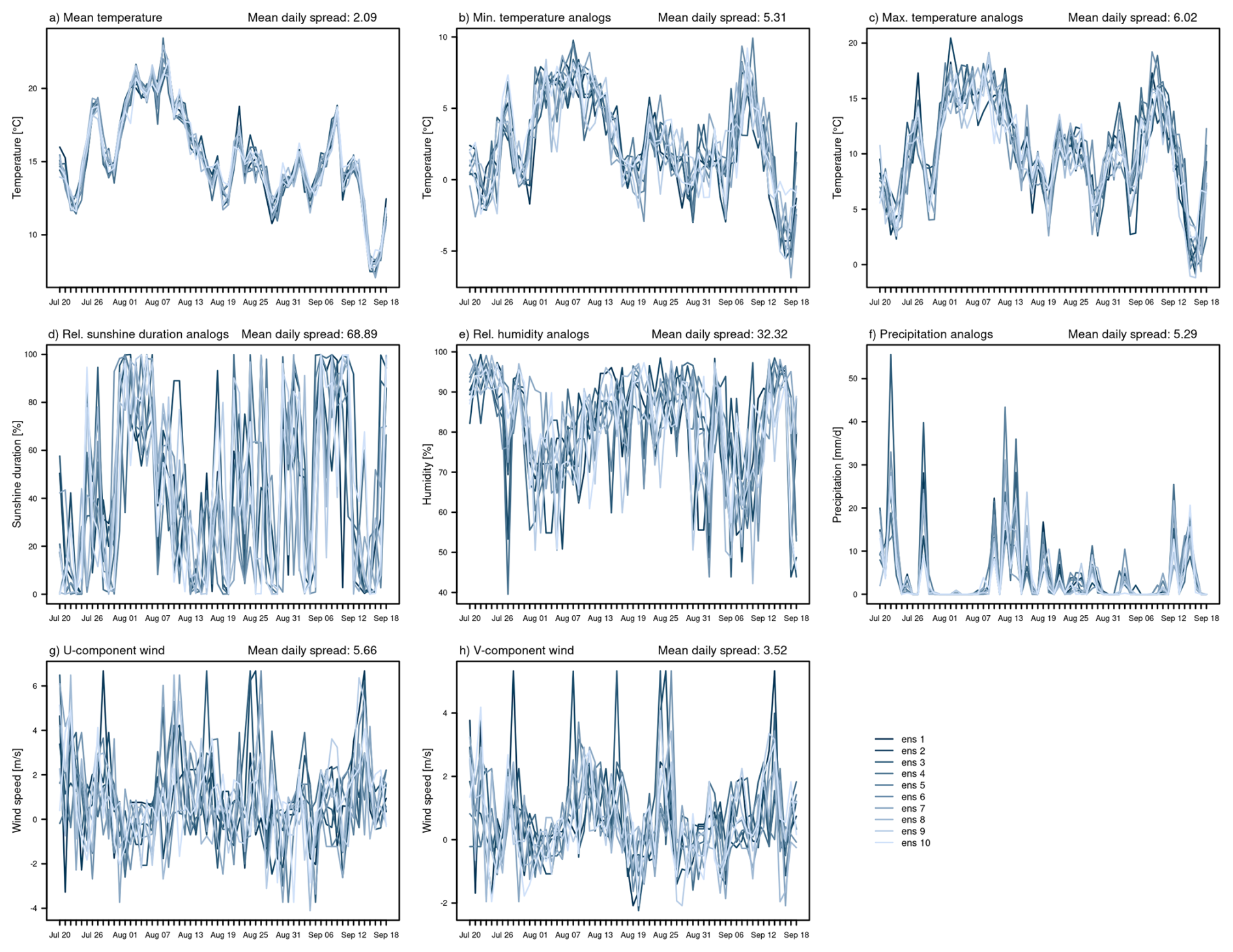
Figure A5 10-member ensemble of the presented variables. For mean temperature, the ensemble after data assimilation is presented. For the other variables, only the ensemble based on analogue days is presented. The spread (max − min ensemble) is shown as the average spread over the example year in 1957. The evaluation was made for the grid cell at 2553500 E, 1183500 N and can vary significantly depending on the area (Swiss coordinate system LV95).