A global eddy splitting and merging trajectory dataset based on satellite altimetry utilizing eddygroup, eddytree and eddygraph

The splitting and merging of mesoscale eddies constitute significant dynamical processes and remain a central subject of investigation in oceanographic research. An eddy is defined as a closed contour derived from satellite altimetry data that encloses a seed point (local extremum), while a closed contour containing multiple eddies and seed points is identified as an eddygroup. The eddytree is a rooted hierarchical tree structure in which eddygroups and eddies are organized by spatial containment. An efficient global algorithm is developed for the identification of mesoscale eddies and eddygroups, and an eddygroup area-based ranking algorithm is further proposed for constructing eddytrees. Compared with existing approaches, the overall computational efficiency is enhanced by a factor of eleven. For eddy tracking, a particle-drift method is applied to track the splitting and merging between eddygroups and eddies at the terminal nodes of the eddytree, which are ultimately connected into eddy directed acyclic graphs (referred to as eddygraphs). Based on these methods, a 31 year (January 1993–December 2023) global dataset of mesoscale eddies and eddygroups, as well as a trajectory dataset of eddy splitting and merging, is constructed. The identification dataset contains 56 948 049 eddies and 29 842 033 eddygroups, from which 12 198 840 eddytrees were constructed. The tracking dataset contains 925 381 eddygraphs associated with splitting and merging events. These datasets provide valuable references for advancing research on ocean dynamics and climate variability. Furthermore, statistical analyses of the 31 year identification results reveal the existence of relatively stable and persistent cyclonic and anticyclonic eddytree structures within the ocean. These structures correspond closely with large-scale ocean circulation patterns: anticyclones dominate in regions of strong western boundary currents; boundaries between cyclonic and anticyclonic eddytrees emerge at confluence zones of warm and cold currents, forming a dipole-like eddytree structure; and island wake regions exhibit von Kármán-type vortex-street structures. Finally, we normalize and characterize the morphological evolution of eddygroups and eddies during splitting and merging processes. The analysis shows that before merging, pairs of eddies typically take on egg-shaped morphologies, which remain after merging, with the smaller eddy corresponding to the sharp pole of the egg-shaped structure. Similarly, before splitting, eddies also exhibit egg-shaped forms, and after splitting, the smaller eddy corresponds to the sharp pole of the pre-split structure. During this process, the research found that the common parent eddygroup plays an important role in the morphology of the splitting and merging events, where the boundary of the resultant eddy after merging is a degeneration of the boundary of the two pre-merging eddies' common parent eddygroup, while before splitting, the boundary of the single eddy evolves into the common parent eddygroup of the two post-splitting eddies. This also reveals the reciprocal nature of the dynamic processes of eddy splitting and merging. The dataset is publicly available via https://doi.org/10.12237/casearth.20250026 (Tian and Kong, 2025).

1 Introduction

Mesoscale eddies, characterized as rotating water masses, are prevalent throughout the global ocean, with horizontal scales ranging from tens to hundreds of kilometres (Chelton et al., 2011b, a; Cheng et al., 2014; Faghmous et al., 2015). They transport water masses and play a crucial role in the redistribution of properties, including heat, salinity, and energy, thereby exerting a substantial influence on global climate variability (Thompson et al., 2014; Dong et al., 2014; Zhang et al., 2014; Xu et al., 2011, 2016). At present, eddy identification methods are generally divided into Lagrangian (Onu et al., 2015; Xia et al., 2022; Jones-Kellett and Follows, 2024) and Eulerian approaches (Chelton et al., 2011b; Faghmous et al., 2015), depending on the coordinate system employed. Lagrangian methods identify eddy structures by analyzing the motion of fluid particles over a finite time interval, typically requiring significant computational resources. Among them, the black-hole eddy method identifies eddies by locating materially closed eddy boundaries based on the theory of Lagrangian coherent structures (LCS) (Tian et al., 2025). The LAVD method detects eddies by computing the Lagrangian-averaged vorticity deviation and identifying fluid structures that rotate coherently around a core over a finite time interval (Tian et al., 2022). In contrast, Eulerian eddy detection methods identify eddies based on instantaneous flow-field properties and are computationally simpler and more efficient. These Eulerian methods are generally classified into three categories: (i) parameter-based approaches, such as the Okubo–Weiss (OW) method (Isern-Fontanet et al., 2003; Chelton et al., 2007; Williams et al., 2011; Xing and Yang, 2021) and the winding–angle (WA) method (Chaigneau et al., 2008); (ii) vector geometry (VG) approaches (Williams et al., 2011; Sadarjoen and Post, 2000); and (iii) approaches based on sea level anomaly (SLA) fields (Chelton et al., 2011b; Faghmous et al., 2015; Liu et al., 2016). Among them, the SLA-based method is less dependent on certain threshold parameters and is suitable for the identification of large-scale eddies. Consequently, it represents the most widely used eddy identification method at present.

Most current eddy-tracking methods treat eddies as independent water masses and primarily concentrate on their emergence and disappearance. In reality, throughout the complete life cycle of an eddy, interactions with other eddies may occur, resulting in splitting and merging events (Isoda, 1994; Fang and Morrow, 2003; Le Vu et al., 2018). Consequently, the investigation of these processes is essential for understanding interactions between eddies. (Yao et al., 2023) examined the vertical structure of mesoscale eddies in the Kuroshio–Oyashio Extension region and showed that although splitting and merging do not introduce new kinds of vertical structures, they can cause large intra-kind variability. To date, research on eddy splitting and merging has primarily concentrated on a few representative cases to assess their impacts. (Schouten et al., 2000) monitored several long-lived eddies and found that splitting and merging influence eddy lifetimes. More recently, (Fu et al., 2023) analyzed the merging processes of typical eddies in the Northwest Pacific and described three stages: the evolution of a single eddy, interactions between eddies, and the formation of the merging eddy. Their study also emphasized the critical role of multi-core eddies and shared contours during the merging process.

In addition, relatively few studies have developed algorithms for the automatic identification and tracking of eddy splitting and merging across basin- to global scales. Li et al. (2016) proposed a Genealogical Evolution Model (GEM), which uses a two-dimensional (2-D) similarity vector to measure the similarity between eddies, and both “parent” and “child” to describe the birth and death of different generations in eddy splitting, thereby enabling the tracking of splitting and merging events in the North Pacific. However, this approach neglects the critical role of eddygroups during these processes. (Tian et al., 2021) introduced the Eddygraph algorithm, which first identifies multi-level eddy structures, constructs eddytrees with eddies, seed points, and multi-core eddies as leaf nodes and eddygroups as intermediate nodes, and then applies a 0.5° search radius to track eddies on subsequent days. Overlapping areas are used to construct segments, which are connected into branches, ultimately forming directed acyclic graphs (Eddy-DAGs) for splitting and merging events. Furthermore, the study confirmed the authenticity of the eddy splitting and merging tracking algorithm based on satellite altimetry data using temperature observations. Yet, this study was limited to the Northwest Pacific and did not extend to global tracking. More recently, Ioannou et al. (2024) presented the TOEddies algorithm for global eddy identification and splitting–merging tracking. This method focuses solely on eddies, linking them into temporal trajectories using similarity parameters such as distance between eddies, Rossby number, and speed radius. Nevertheless, the reliance on subjectively defined parameters constrains the objectivity of the tracking results. Furthermore, this study ignored eddygroups and did not explore the boundary evolution associated with eddy splitting and merging processes.

Although a variety of algorithms have been developed for mesoscale eddy identification and tracking, including those previously mentioned, publicly accessible datasets that provide global records of eddy splitting and merging remain scarce. On the one hand, existing global datasets (Chelton et al., 2011b, a; Pegliasco et al., 2022) focus on eddy identification, with differences mainly arising from the thresholds and criteria used to define mesoscale eddies. These datasets generally do not include information on eddygroups and the associated eddy–eddygroup topological relationships. Moreover, due to computational constraints, datasets capable of representing multi-level eddy structures are typically restricted to regional ocean (Li et al., 2016; Tian et al., 2021), with no equivalent products available at the global scale. On the other hand, datasets that incorporate splitting and merging information, derived from global eddy identification results, often rely on subjectively prescribed thresholds (e.g., overlap area or distance constraints), thereby limiting their objectivity (Li et al., 2016; Tian et al., 2021; Ioannou et al., 2024).

Due to the scarcity of publicly accessible global datasets, comprehensive analyses of mesoscale eddy splitting and merging on a global scale remain limited. From a morphological perspective, (Chen et al., 2021) summarized the characteristic egg-shaped structure of eddies based on a large number of snapshots; (Zhao et al., 2017) demonstrated that in physical systems, vortex-vortex interaction leads to the formation of various patterns, like vortex stripes, labyrinths, deformed lattices, etc. In terms of dynamic morphology, (Fu et al., 2023) investigated the evolutionary processes of several representative merging events, and (Long et al., 2024), through normalized analysis, revealed the “kidney-shaped” evolution of asymmetric dipole (opposite-signed) eddies during gear-like interactions, offering a new perspective for characterizing eddy–eddy interactions. Nevertheless, morphological investigations of the general processes of oceanic eddy splitting and merging – as a key manifestation of like-signed eddy interactions – remain insufficient. Most existing studies have been confined to event-level tracking, lacking systematic exploration of their spatiotemporal evolution.

This study makes the following contributions: (1) We propose an efficient global algorithm for identifying mesoscale eddies and eddygroups, and construct a hierarchical eddy topology (the eddytree). Compared with existing methods, the overall computational efficiency is enhanced by a factor of eleven. In addition, eddy tracking is performed using a Lagrangian particle-drift approach based on eddy centroids, leading to the creation of a splitting and merging tracking algorithm based on the eddy directed acyclic graphs (hereafter referred to as the eddygraphs). (2) Building on the identification and tracking algorithms, we construct the global datasets covering 1993–2023 (31 years), including eddy and eddygroup identifications with their topological structures, as well as a trajectory dataset of eddy splitting and merging events based on particle drifting. (3) Statistical analyses of the identification and tracking results reveal the presence of relatively stationary and persistent cyclonic and anticyclonic eddytree structures throughout the global oceans, most prominently in western boundary current regions. These structures correspond to major circulation features: anticyclonic eddytrees predominate in strong western boundary currents, boundaries between cyclonic and anticyclonic eddytrees appear at warm–cold current confluence zones, and island wake regions exhibit von Kármán-type vortex-street patterns. (4) We normalize and examine the dynamic processes of splitting and merging for eddygroups and eddies of different polarity. The results show that before merging, two eddies typically display near-egg-shaped forms, and after merging, the resultant eddy retains this morphology, with the sharp pole of the egg-shaped structure corresponding to the smaller pre-merger eddy. Before splitting, eddies exhibit near-egg-shaped forms, and after splitting, the two resultant eddies retain this morphology, with the smaller eddy corresponding to the sharp pole of the pre-split structure. During this process, the research found that the common parent eddygroup plays an important role in the morphology of the splitting and merging events, where the boundary of the resultant eddy after merging is a degeneration of the boundary of the two pre-merging eddies' common parent eddygroup, while before splitting, the boundary of the single eddy evolves into the common parent eddygroup of the two post-splitting eddies. For the first time, we reveal the reciprocal nature of eddy splitting and merging processes.

The remainder of this paper is organized as follows. Section 2 describes the datasets and the algorithms used for eddy identification and tracking. Section 3 presents the results in detail, including global statistical analyses and the normalization of typical events. Section 4 discusses the usability of the dataset. Section 5 presents a discussion of the study and outlines future directions.

2 Data and Method

2.1 Data

2.1.1 Absolute dynamic topography data

This study employs absolute dynamic topography (ADT) fields derived from the satellite altimetry product SEALEVEL_GLO_PHY_L4_MY_008_047 for eddy and eddygroup identification as well as eddy tracking. The dataset, originally developed by the French Archiving, Validation, and Interpretation of Satellite Oceanographic data (AVISO) center, is now made available through the Copernicus Marine Environment Monitoring Service (CMEMS; https://resources.marine.copernicus.eu, last access: 30 May 2026). The product is generated through the Data Unification and Altimeter Combination System (DUACS), which merges multi-mission altimetry from satellites including Sentinel-3, the Jason series, Saral/AltiKa, Topex/Poseidon, and Envisat. The dataset spans from 1 January 1993–31 December 2023, with a temporal resolution of one day and a spatial resolution of 0.125°×0.125° covering the global ocean.

2.2 Method

In this study, eddies, multi-core eddies, and seed points are treated as key manifestations of eddy splitting and merging events, while eddygroups serve as important organizing and constraining structures within these processes. A seed point is defined as a local extremum of the ADT field within a 5×5 grid window. The occurrence of a seed point generally indicates that the region is likely located within an eddy or has the potential to develop into an eddy; therefore, the identification of seed points forms the basis for eddy detection. An eddy is characterized by a closed contour that contains a single seed point and concurrently meets specified thresholds for area, amplitude, and shape. The polarity of an eddy is determined by comparing the ADT values within its boundary to those on the boundary: if interior values exceed the boundary value, the eddy is classified as anticyclonic; otherwise, it is classified as cyclonic. An eddygroup is defined as a closed contour region containing two or more objects (seed points, eddies, or nested eddygroups). If the region contains only multiple seed points, it is defined as a multi-core eddy. Applying the same polarity criterion, this study also determines the polarity of an eddygroup. Specifically, the average height of the objects directly contained within the eddygroup is calculated, where the height of seed points, the centroid height of eddies and multi-core eddies, and the boundary height of nested eddygroups are used, respectively. If this average value exceeds the boundary height of the eddygroup, it is classified as an anticyclonic eddygroup; otherwise, it is classified as a cyclonic eddygroup.

To better characterize the hierarchical organization of eddy structures, we introduce the concept of an “eddytree,” defined as a spatial topological tree wherein each node corresponds to a closed contour or a point. Within this framework, the outermost eddygroup is regarded as the root node, intermediate eddygroups serve as internal nodes, and eddies, multi-core eddies, and seed points are treated as leaf nodes. Figure 1 illustrates an example of such a structure, consisting of a root node (eddygroup 1), internal nodes (eddygroups 2–5), and leaf nodes (eddies 1–5, multi-core eddy 1, and seed points 1–3). The polarity of an eddytree is defined by the polarity of its root eddygroup: trees rooted in anticyclonic eddygroups are classified as anticyclonic eddytrees, and those rooted in cyclonic eddygroups are classified as cyclonic eddytrees. Nodes with a direct containment relationship are considered to have a parent–child link: the encompassing eddygroup serves as the parent node, while the enclosed eddygroups, eddies, or seed points constitute its child nodes. For example, in Fig. 1, eddygroup 1 has as its child nodes eddygroups 2–4, seed point 1, and eddy 1, while eddygroup 1 acting as their parent nodes. An eddytree has a unique root node, but the number of internal and leaf nodes may vary.

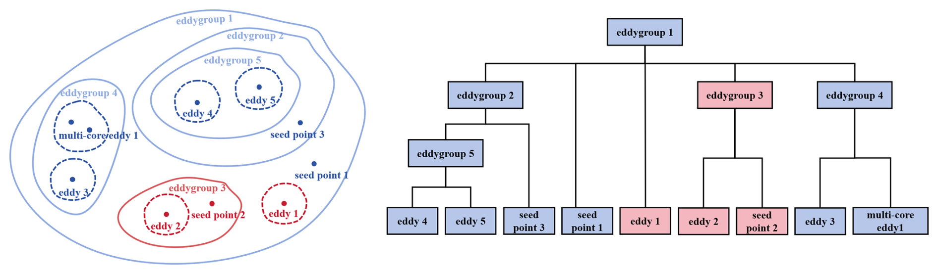
Figure 1 Schematic illustration of seed points, eddies, multi-core eddies, eddygroups, and the eddytree. In the left panel, red and blue dashed lines represent anticyclonic and cyclonic eddies or multi-core eddies, respectively, whereas red and blue solid lines denote anticyclonic and cyclonic eddygroups, respectively. Red and blue points represent anticyclonic and cyclonic seed points, respectively. The right panel shows the nested relationships as illustrated in the left panel, blue and red background rectangles denote cyclonic and anticyclonic polarities, respectively.

Figure 2 shows the identification results of eddies and eddygroups on 1 January 2020, for the global ocean and the northwestern Pacific region. Approximately 40 % of the global ocean surface is covered by eddies and eddygroups. And this figure shows that eddytrees of different polarities are distributed on both sides of the Kuroshio Extension current.

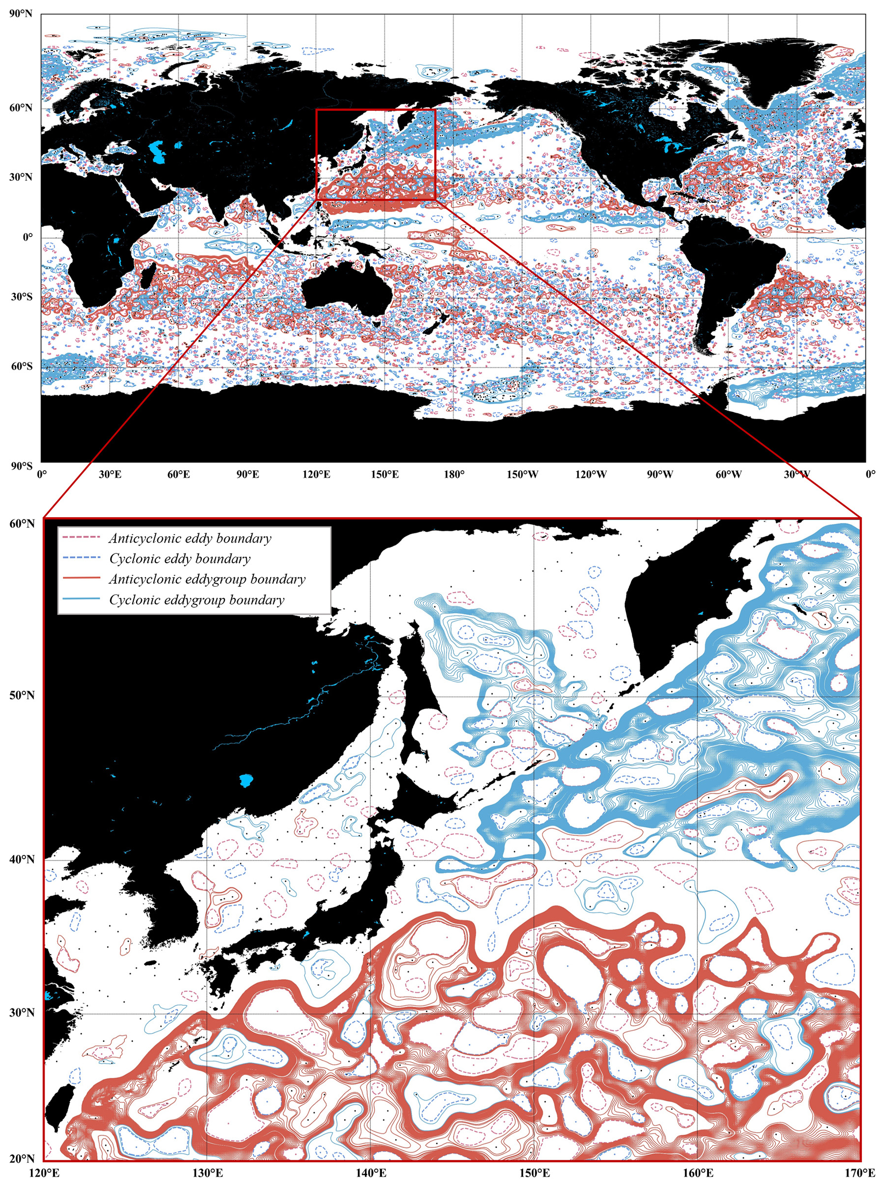
Figure 2 Polarity distribution of eddies and eddygroups on 1 January 2020. In this figure, red and blue dashed lines denote the boundaries of anticyclonic and cyclonic eddies, respectively, while red and blue solid lines denote anticyclonic and cyclonic eddygroups, respectively.

As a fundamental component of the eddytree, eddygroups can contain other eddygroups, eddies, multi-core eddies, and seed points, thereby reflecting the topological relationships among eddies. Eddies are compact, rotating fluid masses in the ocean, implying that their splitting and merging require certain time intervals, during which the organizational and constraining functions of eddygroups become particularly important.

Taking the merging of two eddies and the splitting of an eddy into two eddies as examples, as illustrated in Fig. 3, the merging of two eddies involves an initial approach and subsequent enclosure within a common eddygroup. Within this closed structure, the eddies interact to form a multi-core eddy, which ultimately merges into a single eddy. Conversely, the splitting of an eddy begins with its evolution into a multi-core eddy, wherein different seed points develop into independent eddies. Simultaneously, the boundary of the original multi-core eddy evolves into an eddygroup, leading eventually to the complete division into two eddies. It indicates the critical role of common eddygroup boundaries in the processes of eddy splitting and merging, and underscores that accurate identification of both eddies and eddygroups is a prerequisite for tracking.

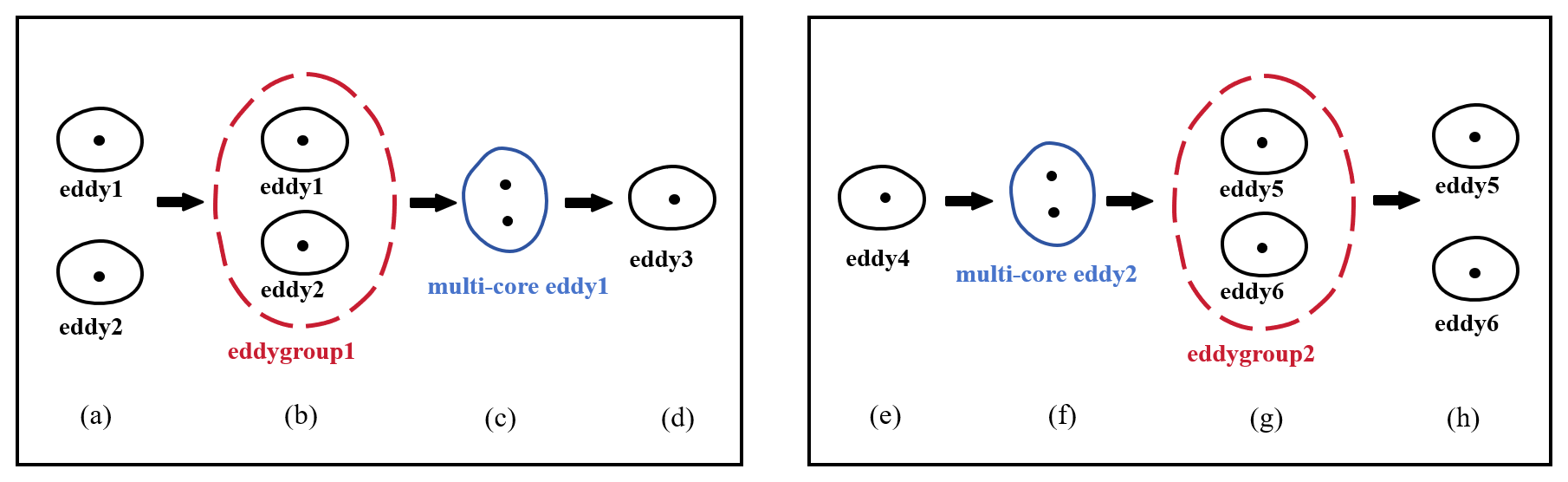
Figure 3 Illustration of eddy merging and splitting processes. The left panel (a–d) shows a merging event: (a) eddies 1 and 2 gradually approach each other; (b) both eddies become enclosed within a common eddygroup 1, delineated by a red boundary; (c) within this enclosed structure the eddies continue to interact and evolve into multi-core eddy 1; (d) the seed points of this multi-core eddy 1 merge into a single seed point, forming eddy 3. The right panels (e–h) illustrate a splitting event: (e–f) multiple seed points appear within eddy 4, producing multi-core eddy 2; (g) these seed points gradually separate and develop into eddies 5 and 6, accompanied by the formation of common eddygroup 2 (red boundary); (h) the structure ultimately splits into eddies 5 and 6. Seed points are indicated by black dots throughout.

A segment is defined as the survival relationship between eddies observed over two consecutive days. During the eddy life cycle, four distinct states are identified: live segment (representing eddy survival), dead segment (representing eddy decay), merged segment, and split segment (Fig. 4). The tracking procedure adopted in this study proceeds as follows: first, eddy segments are tracked between two consecutive time steps (i.e., successive days); next, all live segments are concatenated end-to-end to generate eddy survival trajectories, hereafter referred to as branches; finally, branches that terminate in merging or splitting events are further connected to construct complete eddy trajectories. Owing to the unidirectionality of time, the resulting trajectories constitute eddy directed acyclic graphs (hereafter termed eddygraphs).

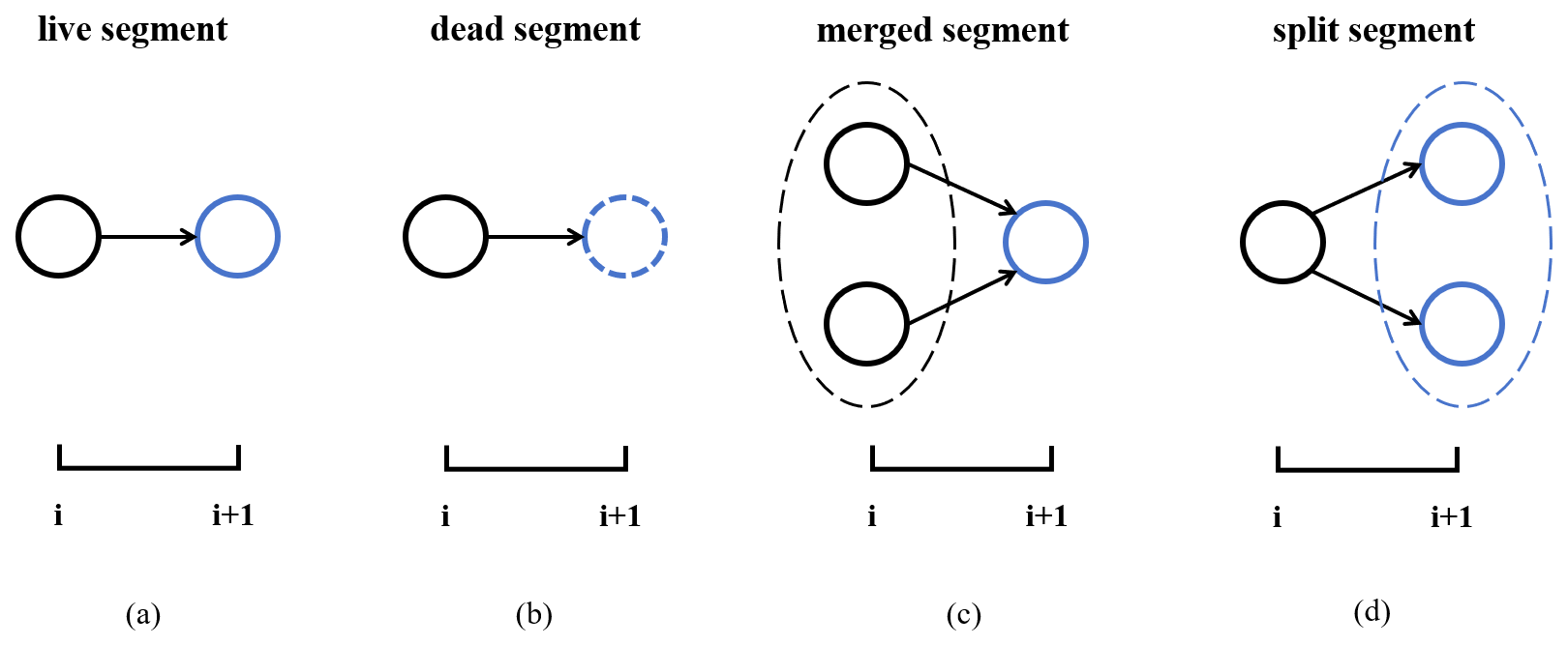
Figure 4 The four states of eddy evolution. Black and blue circles denote eddies observed on day i and day i+1, respectively. Dashed ellipses in panels (c, d) indicate the common eddygroup boundaries. The subfigures illustrate: (a) the continuity of the same eddy across two consecutive time steps, identified as the live segment; (b) the absence of a corresponding eddy in the subsequent time step, identified as the dead segment; (c) the merging of an eddy from day i into another at day i+1, identified as the merged segment; and (d) the splitting of an eddy from day i into two distinct eddies at day i+1, identified as the split segment.

2.2.1 Eddy and eddygroup identification algorithm

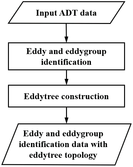
The identification of eddies, eddygroups, and their associated topological structures in this study is conducted through two main steps, as shown in Fig. 5. Initially, following data input, eddies and eddygroups are first identified. Subsequently, the topological structure is constructed, yielding the final multi-level identification results for eddies and eddygroups.

Figure 5 Overall flowchart of the eddy and eddygroup identification algorithm.

Eddy and eddygroup identification

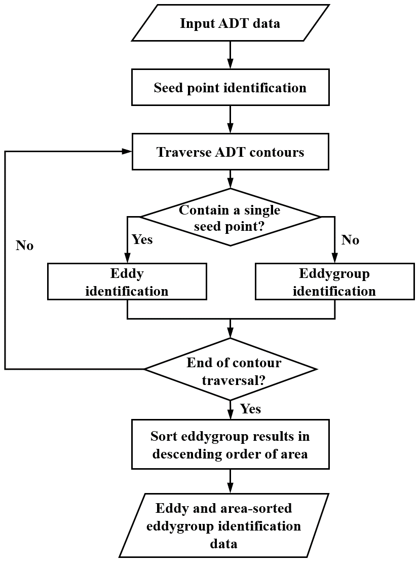
The algorithmic steps for the identification of eddies and eddygroups are depicted in Fig. 6. Initially, seed points are detected, followed by the extraction of closed contours. For each contour, the quantity and indices of enclosed seed points are recorded to distinguish between cases: contours enclosing a single seed point are identified as eddies, while those containing multiple seed points are identified as eddygroups. Prior to producing the final output, the identified eddygroups are sorted in descending order based on area to facilitate subsequent construction of the eddytree.

Figure 6 Flowchart of the eddy and eddygroup identification algorithm.

The criteria for defining eddy boundaries follow standards similar to those of (Tian et al., 2021; Mason et al., 2014), with the primary distinction arising from the spatial resolution of the dataset. The number of pixels I is used to constrain the area of mesoscale eddies. Referring to the parameter values adopted in previous studies, I between 20 and 4000 in this study; this number increases as the grid resolution becomes finer. The shape error is introduced to constrain the morphological characteristics of eddies and is defined as the ratio of the total area difference between the closed contour and its fitted circle to the area of that circle. Thus, a smaller shape error indicates that the eddy's shape is closer to an ideal circle. In addition, the constraint on eddy amplitude is related to the contour generation interval chosen for this study, which is set as 0.5 cm; therefore, the eddy amplitude is required to exceed at least two contour intervals. The size of the seed point detection window is also related to the spatial resolution of the data: higher spatial resolution leads to a denser data grid and a larger number of pixels within the seed point detection window. Specifically, an eddy is required to meet the following conditions:

1. Contain a single local maximum or minimum.

2. Include I grid cells (0.125°×0.125°), where $\mathrm{20}\le I\le \mathrm{4000}$.

3. The shape error ≤55 %.

4. The amplitude, defined as the absolute difference in ADT height between the local extremum and the eddy boundary, must be at least 1 cm.

Eddytree construction

The procedure for constructing eddytrees using the area-sorting method is illustrated in Fig. 7. Initially, the identified eddies and the area-sorted eddygroups are input, with the largest eddygroup designated as the root node of the initial eddytree. Subsequently, the remaining eddygroups and eddies are traversed sequentially. If a given target is not contained by any existing root node, a new eddytree is initialized for that eddygroup, or the eddy is recorded as an independent entity. Conversely, if the target is contained within an existing root node, the containment relationships are evaluated within that tree: starting from the root, the hierarchy is examined level by level until the target is no longer enclosed by any eddygroup, at which stage it is inserted as a node at that level. Upon completion of this traversal, the eddytree identification result for the given day is obtained.

Figure 7 Flowchart of the eddytree construction algorithm.

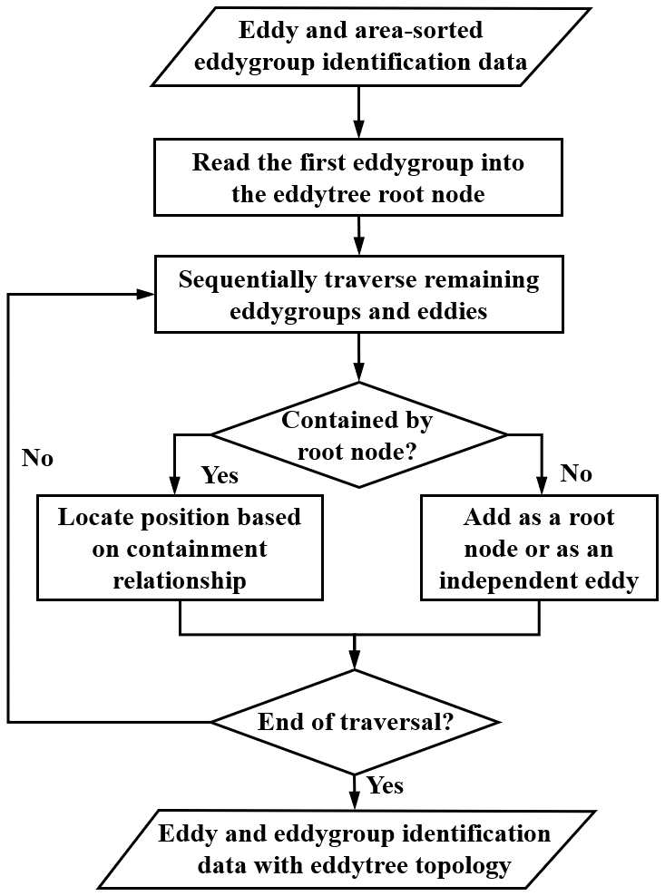
In general, root nodes corresponding to larger eddygroups tend to exhibit more complex hierarchical structures, encompassing a greater number of internal and leaf nodes. The area-sorting-based eddytree construction algorithm takes full advantage of this parameter by establishing larger root nodes first in descending order of area. This strategy allows the assignment of subsequent eddygroups and eddies at shallower hierarchical levels, thereby minimizing the necessity for backtracking and redundant comparisons. For independent eddies, verification is limited to confirming their exclusion from all root nodes, obviating the need for deeper containment checks within each eddytree. This approach consequently reduces computational cost and enhances overall efficiency.

In contrast to existing “identify-while-building” algorithms (Tian et al., 2024), the present study separates the construction of the eddytree from the identification phase. The identification procedure involves only a linear traversal during which essential information is recorded. Subsequently, multi-level eddy structures are generated in a relatively straightforward manner based on area sorting. This separation strategy reduces the overall time complexity from O(n²) to O(nlog n), thereby decreasing the average daily runtime from 480–43 min and enhancing efficiency by approximately a factor of eleven. The computer running the algorithm is configured with an Intel^® Core™ i5-12400F CPU and compiled and implemented in Python 3.8 (Anaconda 3).

2.2.2 Eddygraph construction using particle-drift tracking algorithm

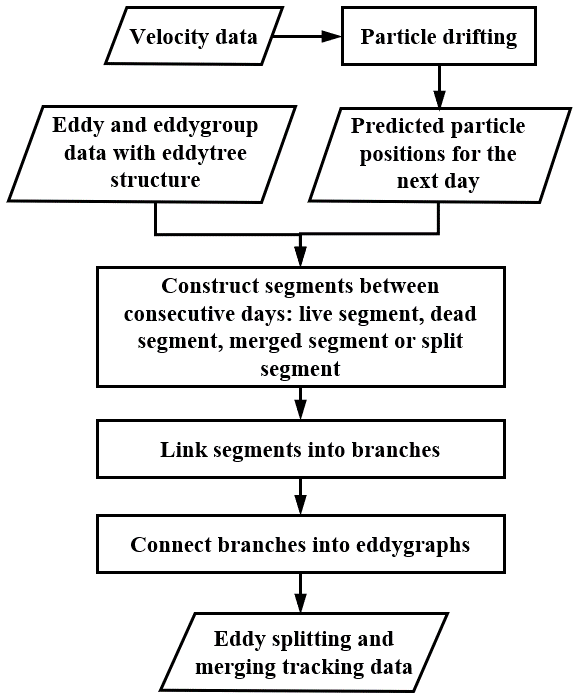
The processes of eddy splitting and merging are tracked using a Lagrangian particle-drift approach, as outlined in the flowchart presented in Fig. 8. This procedure consists of three main steps: (1) establishing segments between consecutive days through particle drifting; (2) linking segments into branches; and (3) connecting branches to form eddygraphs.

Figure 8 Flowchart of the eddy splitting and merging tracking algorithm

Segment construction through particle drifting

In this study, the meridional and zonal components of the absolute geostrophic velocity are used to advect all eddy centroids and associated seed points from day i forward, employing a one-day integration step to predict their positions on day i+1. The Lagrangian particle-drift approach provides a realistic representation of particle motion in the ocean (Haller, 2015; Van Sebille et al., 2018). Due to the substantial number of particles tracked on a daily scale, only the centroid of each eddy is advected as its representative particle (Jones-Kellett and Follows, 2024).

The process of constructing segments based on particle-drift predictions is illustrated in Fig. 9. Segment classification depends on the quantity and distribution of predicted particle positions that fall within eddies or multicore eddies on day i+1: If the predicted position of an eddy centroid or a seed point on day i falls within an eddy on day i+1, the state is classified as a live segment; If the predicted positions of two objects (either eddy centroids or seed points) on day i fall within the same eddy on day i+1, the state is classified as a merged segment; If the seed points from a multicore eddy on day i are advected into distinct eddies on day i+1, the state is classified as a split segment; Finally, if the predicted position of a particle from day i does not fall within any eddy on day i+1, the corresponding eddy or seed point is designated as a dead segment.

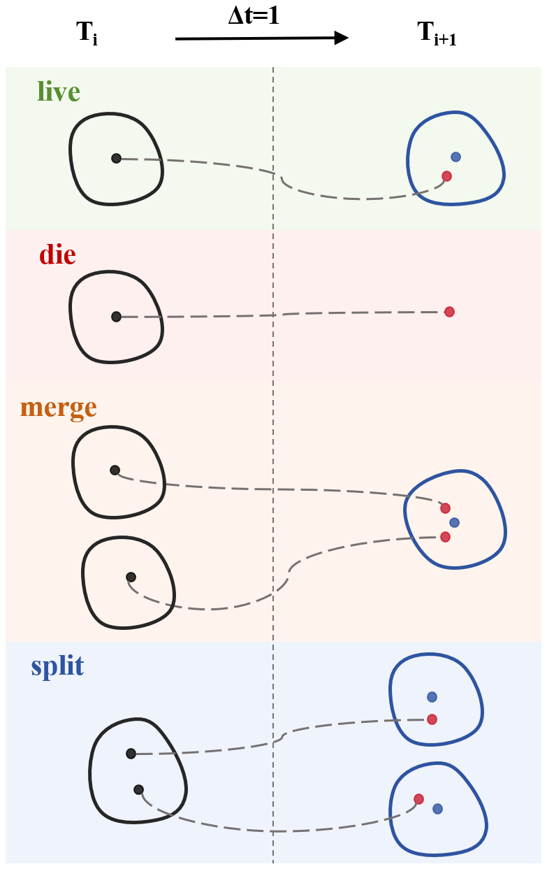
Figure 9 Schematic illustration of the segment construction. The black closed contours represent eddies on day i, and the black dots denote the eddy centroids or seed points of multi-core eddies on day i. The blue closed contours represent eddies on day i+1, and the blue dots denote the eddy centroids on day i+1. The red dots represent predicted particle positions on day i+1, advected from day i by particle drifting.

Branch construction

A branch is defined as a single survival trajectory formed by temporally consecutive live segments that also exhibit spatial overlap, connected in chronological order. To construct branches, the set of segments from day i to day i+1 is first examined to extract live segments. Since each segment records the survival relationship of an eddy between two consecutive days, the surviving target identified in the segment on day i can be used to link the live segments from day i to day i+1. Following the same rule, the live segments between day i+1 and day i+2 are then connected, and this procedure continues sequentially, linking live segments from consecutive days into a continuous trajectory until no corresponding live segment can be found on the following day. The resulting branches may originate from three cases: a newly generated eddy, a child node eddy produced by splitting, or an eddy formed by merging. The termination points of branches likewise correspond to three cases: disappearance on the subsequent day, splitting, or merging (Fig. 10a). Finally, by connecting all qualifying live segments, continuous branches are obtained, as illustrated in Fig. 10b.

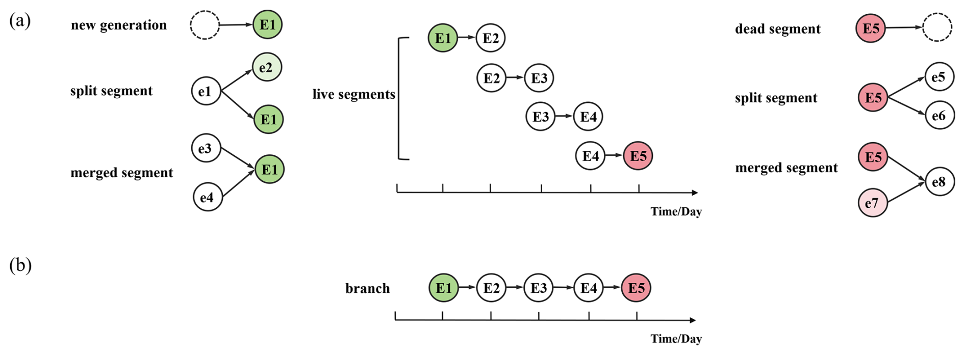
Figure 10 Illustration of constructing a branch from segments. In panel (a), E1–E5 represent four live segments, which are sequentially connected to form the branch shown in panel (b). As the branch origin, E1 may originate from three cases: it may result from the splitting of e1 in the previous time step, from the merging of e3 and e4, or from the generation of a new eddy. Correspondingly, as the branch terminus, E5 may correspondingly end in one of three ways: disappearance in the next time step, splitting into e5 and e6, or merging with e7.

Eddygraph construction

Branches are connected into a complete eddygraph through splitting and merging relationships at their endpoints. For example, if a branch terminates with a merging event, there must exist other branches that merge into the same target eddy at the same time. Conversely, if a branch terminates with a splitting event, multiple new eddies are generated on the next day, which are then used to establish connections with the corresponding branches on that day. As illustrated in Fig. 11, the branches depicted in the left panel are linked by their segment relationships to form a single eddygraph.

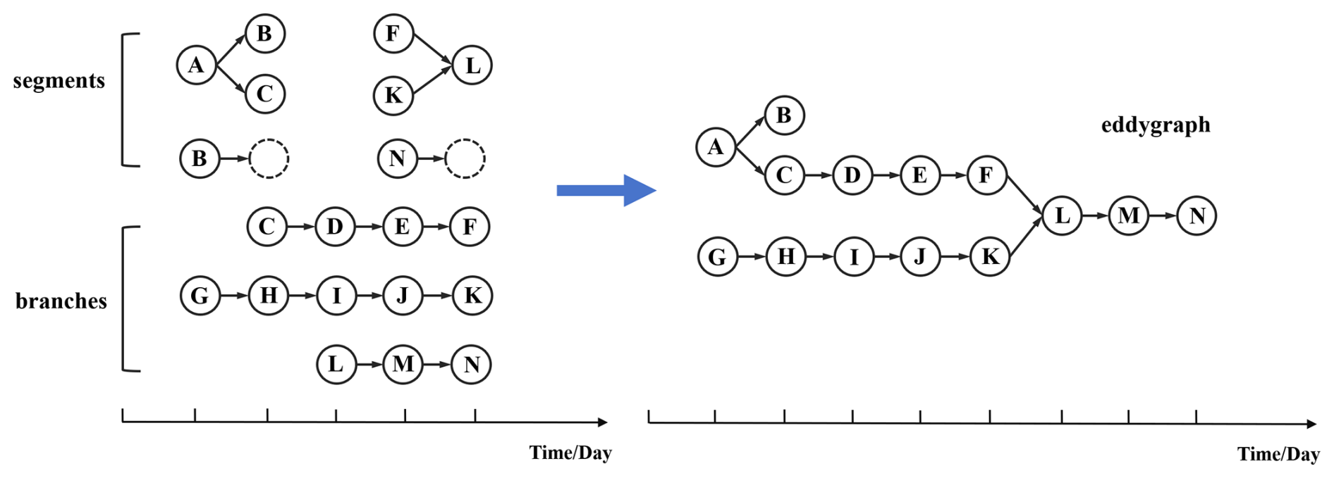
Figure 11 Illustration of eddygraph construction from branches. In the left panel, eddy A splits into B and C, while F and K merge to form eddy L. The trajectories C–F, G–K, and L–N represent three distinct branches. The right panel shows the integration of the branches from the left panel into a complete eddygraph.

Tracking results

Figure 12 presents representative eddygraphs of cyclonic and anticyclonic splitting and merging events. Panels 12a and b illustrate trajectories of typical anticyclonic and cyclonic cases, respectively. For each event, the upper subpanel presents all involved branches, while the lower subpanel shows the connections among these branches through splitting and merging, thereby constructing a complete eddygraph. In Fig. 12a, the easternmost anticyclonic eddy originated on 2 January 2023, merged with another eddy on 24 January. It subsequently split into two eddies on 15 February. Of these, the southern eddy died on 26 June, while the northern one underwent another merging event on 25 June and ultimately died on 11 September, with a total lifetime of 253 d. In Fig. 12b, the eastern eddy formed on 1 January 2022, experienced a splitting event on 5 May. Among the two resultant eddies, one died on 24 May, while the other merged on 17 June with an eddy formed on 22 March. This merged eddy finally died on 8 September, with a total lifetime of 251 d. These examples demonstrate that by incorporating splitting and merging relationships, the tracking method links branches that would otherwise remain disconnected. Compared to conventional tracking approaches that consider only eddy survival and death, this method yields extended lifetimes and more coherent trajectories.

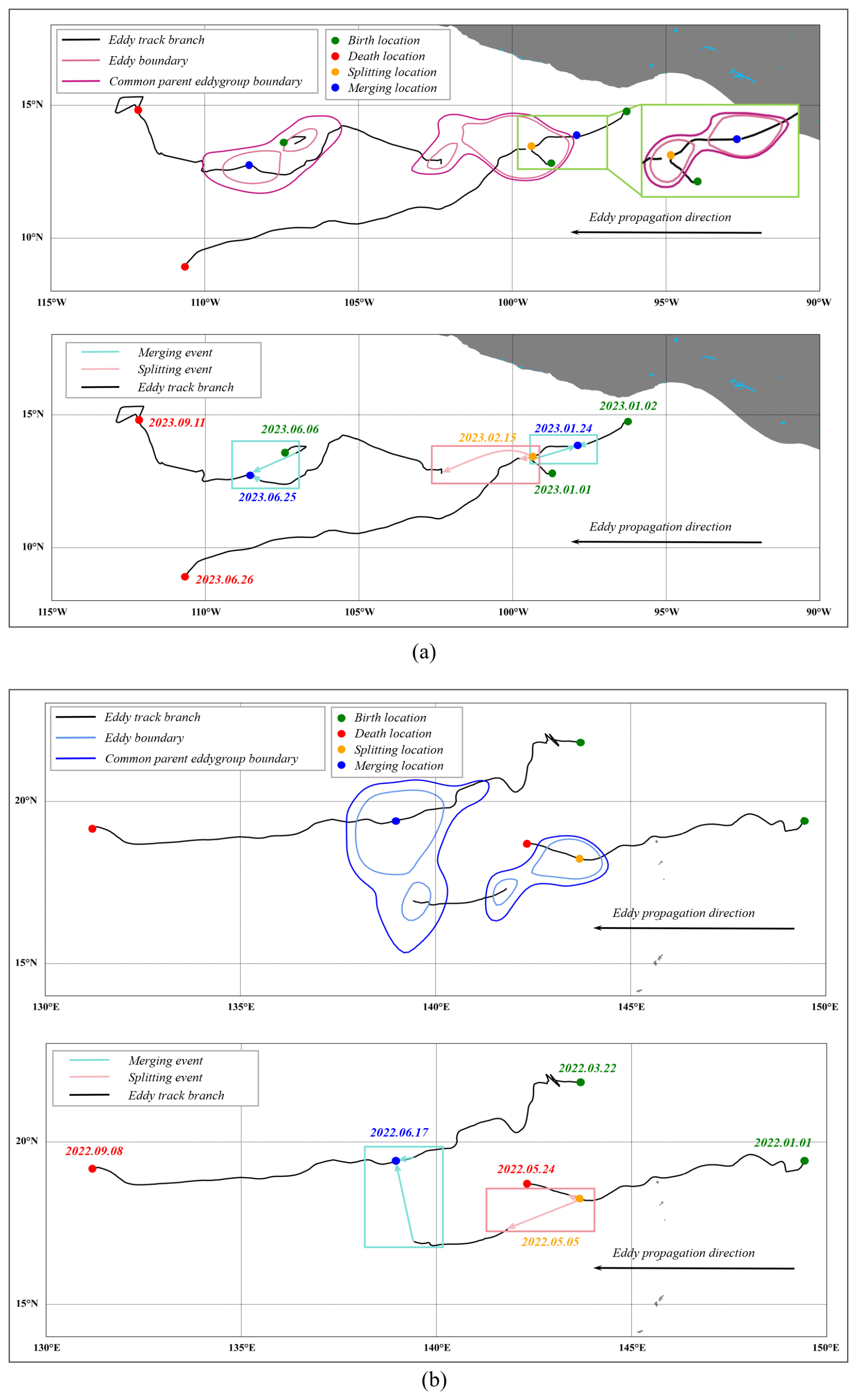
Figure 12 Representative eddygraphs of splitting and merging events. Panel (a) shows a typical anticyclonic eddygraph, while panel (b) depicts a typical cyclonic eddygraph. Green and red dots indicate the birth and death locations of eddies, respectively, while yellow and blue dots denote the positions where splitting and merging occur. Pink and cyan boxes highlight centroid displacements associated with splitting and merging, respectively. The light pink and light blue closed contours represent the boundaries of anticyclonic and cyclonic eddies, respectively, either after splitting or before merging, while the deep pink and deep blue closed contour represents the boundaries of anticyclonic and cyclonic common parent eddygroup, respectively, shared by the two eddies (pre-split or post-merge). The dates marked in green, red, yellow, and blue indicate the timing of eddy birth, death, splitting, and merging, respectively.

In addition, the eddy boundaries depicted in the figure show that the two eddies before merging and after splitting differ in area. During merging, the branch corresponding to the larger eddy exhibits stronger continuity with the post-merger branch. Similarly, in splitting events, the pre-split eddy is more strongly connected to the branch of the larger post-split eddy. To further investigate this behavior, centroid positions were statistically analyzed across all events. Results show that in 91.8 % of merging cases, the centroid of the post-merger eddy is closer to that of the larger pre-merger eddy, while in 92.5 % of splitting cases, the centroid of the pre-split eddy is nearer to that of the larger post-split eddy. These findings indicate that the larger eddy tends to dominate the splitting and merging processes, effectively functioning as the primary entity in such events.

3 Result

The tracking algorithm generated 925 381 eddygraphs from January 1993 through December 2023, within which each eddygraph experienced an average of 8.3 merging events and 3.4 splitting events. Among these, merging events involving two eddies or seed points account for 91.48 % of all merging events, whereas events splitting into two objects account for 95.87 % of all splitting events.

3.1 Statistical characteristics of eddy identification

3.1.1 Global distribution of eddies

Figure 13 presents the annual mean spatial distribution of eddies over the 31 year period. The spatial patterns indicate that eddies are predominantly concentrated along oceanic boundaries and in mid–high latitude regions, whereas their occurrence is relatively sparse in equatorial zones.

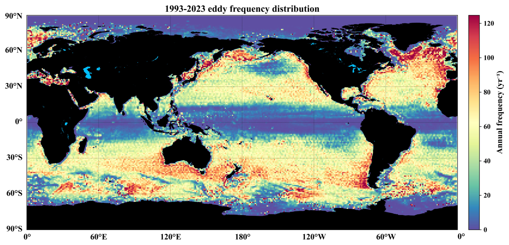
Figure 13 Annual average frequency of eddy occurrence from 1993–2023. The distribution is derived from statistics on a 1°×1° grid.

3.1.2 Global distribution of eddytrees

Inspection of the eddy and eddygroup distribution (Fig. 2) reveals that in some regions, eddygroups with the same polarity tend to cluster. According to our statistics, the mean areas of the anticyclonic eddygroup south of the Kuroshio Extension, the cyclonic eddygroup north of the Kuroshio Extension, the anticyclonic eddygroup south of the Gulf Stream, the cyclonic eddygroup north of the Gulf Stream, and the anticyclonic eddygroup near the Brazil Current are approximately 8.67 million km² (the anticyclonic eddygroup south of the Kuroshio Extension), 4.45 million km² (the cyclonic eddygroup north of the Kuroshio Extension), 7.30 million km² (the anticyclonic eddygroup south of the Gulf Stream), 3.35 million km² (the cyclonic eddygroup north of the Gulf Stream), and 5.05 million km² (the anticyclonic eddygroup near the Brazil Current), respectively. Among them, the largest eddygroup occurred on 8 October 1994 south of the Kuroshio Extension, with an area exceeding 19.64 million km². To quantify the long-term spatial distribution, the daily polarity of the root eddygroups of eddytrees was accumulated over the period 1993–2023 on a 1°×1° grid: grid cells covered by anticyclonic eddytree roots were assigned a value of +1, and those covered by cyclonic roots were assigned a value of −1. The accumulated values were then averaged annually. The results reveal a stable regional preference in eddytree polarity across the global ocean, and the annual-mean distribution of eddytree polarity exhibits a strong correspondence with large-scale ocean circulation. Figure 14 presents the annual-mean distribution of eddytree polarity superimposed on the large-scale ocean circulation, from which it can be seen that: (1) In western boundary regions, strong currents constrained by continental margins – such as the 3 – Kuroshio, 4 – Gulf Stream, 6 – Caribbean Current, 9 – East Madagascar Current, 10 – Agulhas Current, and 11 – Brazil Current – are associated with values exceeding $+\mathrm{300}{\mathrm{yr}}^{-\mathrm{1}}$ (shown in dark red), indicating a persistent dominance of anticyclonic eddytrees; (2) in frontal zones where strong cold and warm currents meet, such as the Oyashio–Kuroshio (1–3) and Labrador–Gulf Stream Current (2–4) confluence zones, a distinct boundary between cyclonic and anticyclonic eddytrees is observed, forming a dipole-like eddytree structure. This boundary extends into the interior ocean and gradually weakens; (3) in open-ocean regions, island topography such as the Hawaiian Islands obstructs the flow, resulting in von Kármán-type vortex-street structures in the wake region of the islands (as shown in Fig. 14b); and (4) within the interior ocean, polarity boundaries are typically associated with stable large-scale currents, including the 5 – North Equatorial Current, 7 – Equatorial Counter Current, 8 – South Equatorial Current, and 12 – Antarctic Circumpolar Current.

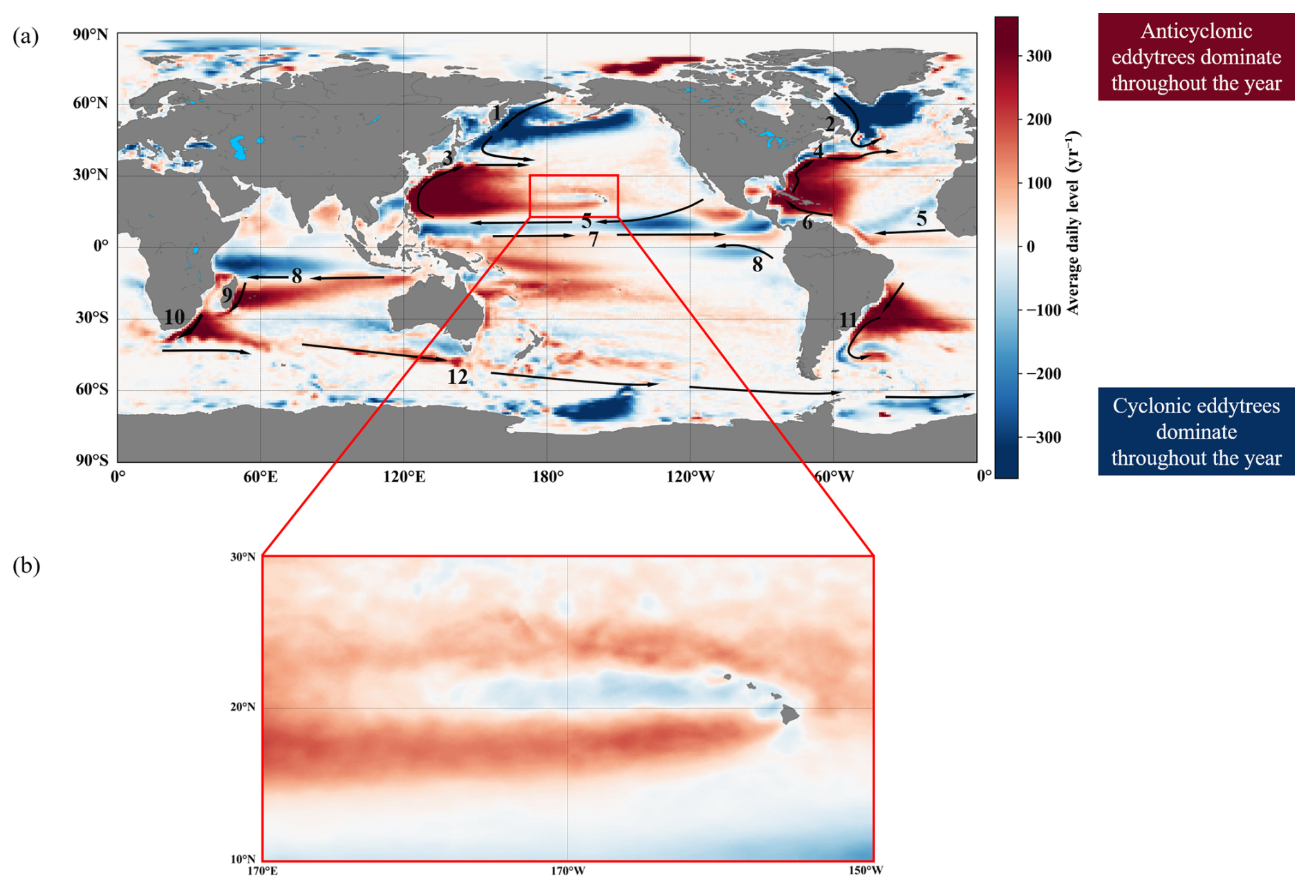
Figure 14 Annual average distribution of eddytree root polarities and associated ocean circulation. In panel (a), Numbers indicate: 1 – Oyashio Current, 2 – Labrador Current, 3 – Kuroshio, 4 – Gulf Stream, 5 – North Equatorial Current, 6 – Caribbean Current, 7 – Equatorial Counter Current, 8 – South Equatorial Current, 9 – East Madagascar Current, 10 – Agulhas Current, 11 – Brazil Current, 12 – Antarctic Circumpolar Current. Panel (b) shows a zoomed-in view of the annual mean distribution of eddytrees near the Hawaiian Islands.

3.2 Splitting and merging processes of same-polarity eddies based on eddygraphs

3.2.1 Statistical analyses of splitting and merging events

Based on the trajectory dataset, the occurrence frequency of eddy splitting and merging events exhibits distinct spatial characteristics. As shown in Fig. 15, the annual average frequency of these events is relatively high in mid- to high-latitude regions, while much lower frequencies are found in low-latitude waters, particularly within the equatorial belt. This spatial pattern is broadly consistent with the distribution of eddies. High-frequency regions are concentrated along the North Pacific margin and central basin, the central South Pacific, the southeastern waters off Australia, the western North Atlantic (especially the Gulf of Mexico and its extension), and the southern Indian Ocean. These regions are characterized by strong eddy kinetic energy, intense shear associated with boundary currents, and pronounced frontal instabilities, all of which enhance the probability of eddy–eddy interactions and thereby lead to a higher frequency of splitting and merging events.

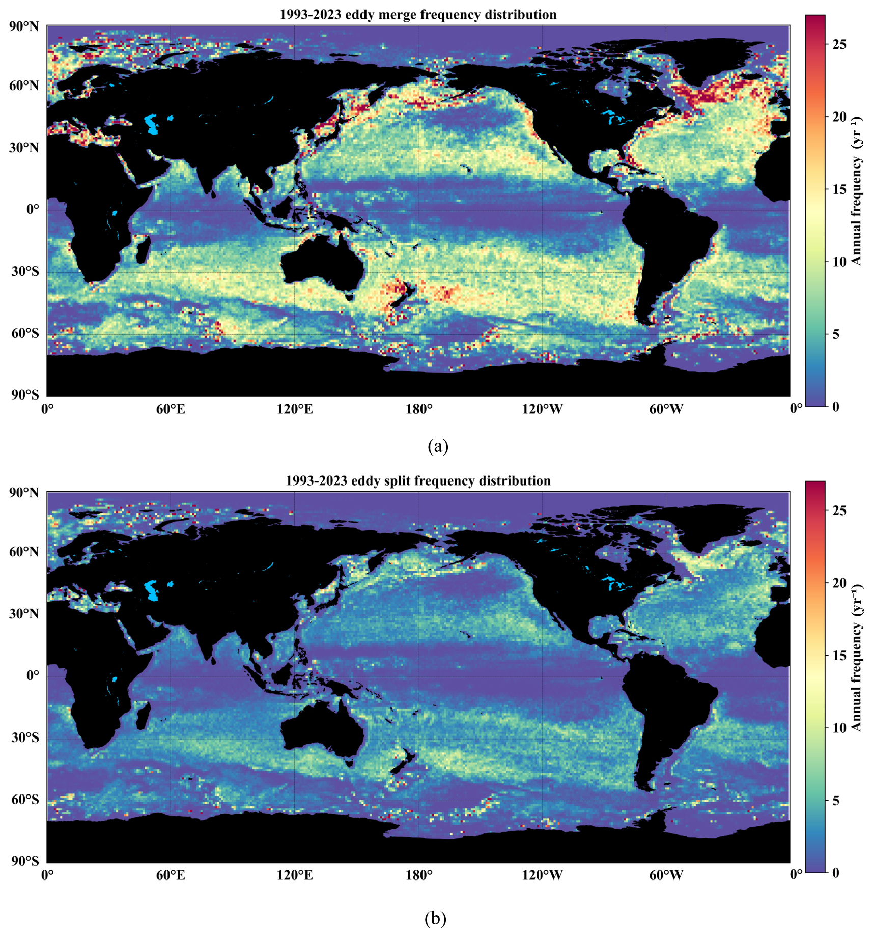
Figure 15 Annual average distribution of global eddy splitting and merging events. The distribution is derived from statistics on a 1°×1° grid. Panel (a) shows the frequency distribution of eddy merging events during from 1993–2023, while panel (b) shows the frequency distribution of eddy splitting events over the same period.

To examine this difference in detail, the occurrences of both types of events were accumulated within each 1° latitude band (Fig. 16). The result indicates that merging events are roughly three times more frequent than splitting events. This pattern may be influenced by survivor bias, as the limited resolution of current satellite altimeters hampers the detection of smaller eddies generated through splitting. Overall, the Southern Hemisphere exhibits a higher frequency of events compared to the Northern Hemisphere, while event counts near the equator remains close to zero. This latitudinal contrast is consistent with spatial distribution of eddies: The Southern Hemisphere has a larger oceanic area and hence more eddies, whereas in equatorial waters eddies are scarce, leading to infrequent splitting or merging occurrences.

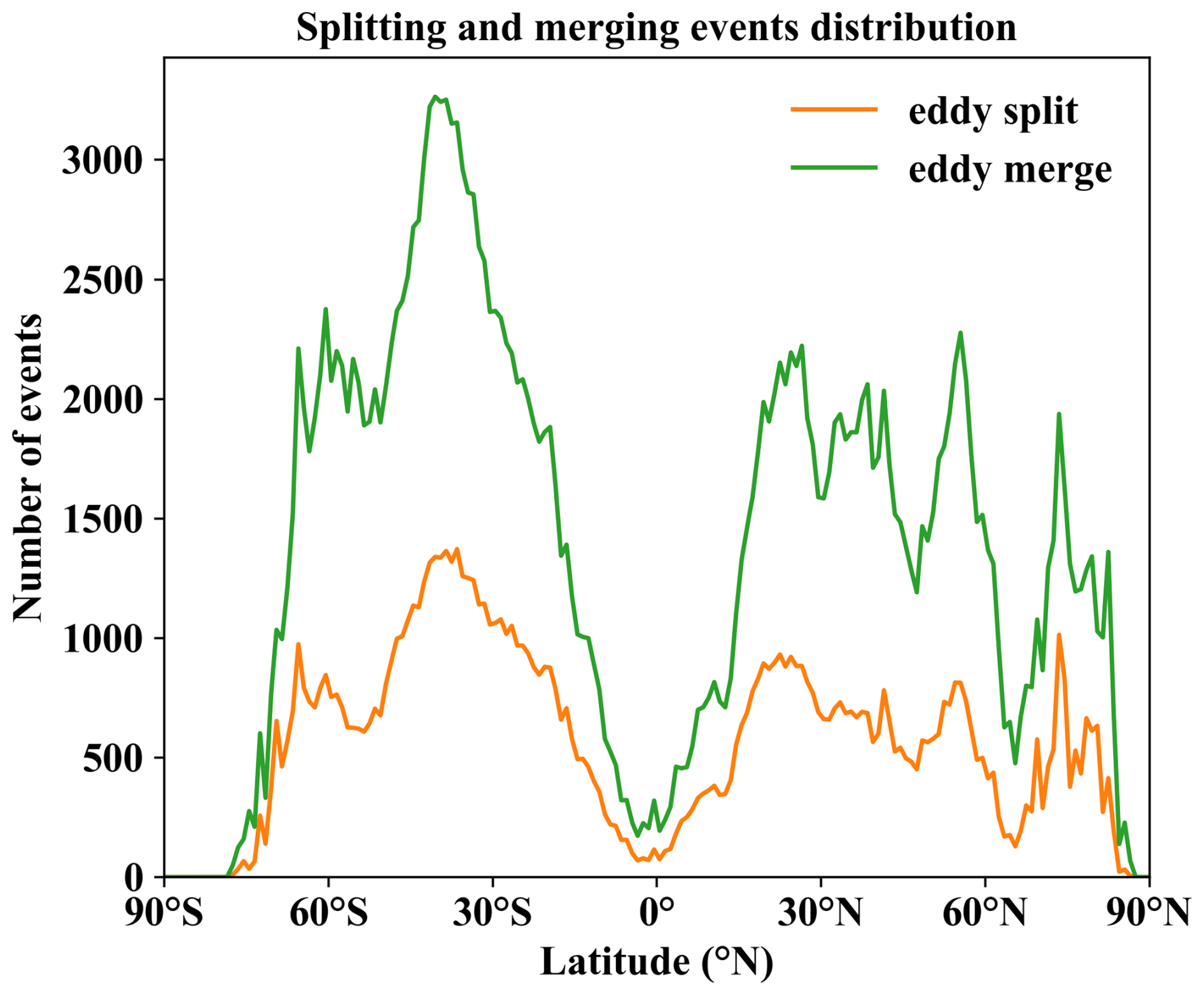
Figure 16 Cumulative eddy splitting and merging events categorized by 1° latitude bands, 1993–2023. The orange and green curves represent splitting and merging events, respectively.

3.2.2 Morphological characteristics of eddy splitting and merging processes

Examples of typical events

Along with extracting representative splitting and merging events, the study examined the associated ADT background fields to visualize the evolution of eddies before and after the events. The analysis reveals that splitting and merging are gradual processes rather than instantaneous transitions. In stable merging cases, two eddies progressively approach one another and develop an egg-shaped geometry. In this configuration, their sharp poles face each other, while their dull poles are oriented outward. They then finally combining into a single eddy (Fig. 17a and b). In stable splitting cases, an eddy initially evolves into a multi-core structure; after splitting, the two resultant eddies gradually separate, again exhibiting paired egg-shaped structures with their sharp poles directed toward one another (Fig. 17c and d).

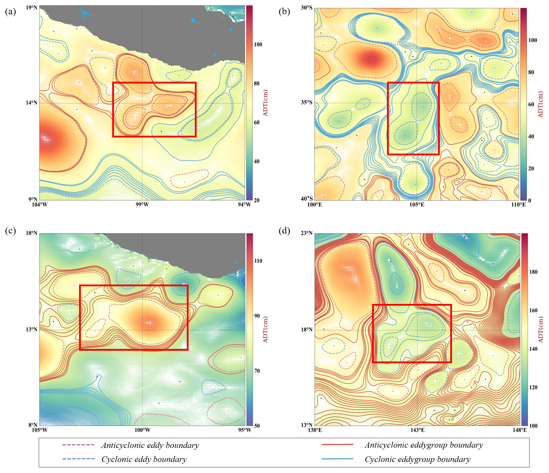
Figure 17 Examples of eddy states before merging and after splitting. Panel (a) highlights two anticyclonic eddies prior to merging, shown within the red box; panel (b) highlights two cyclonic eddies prior to merging; panel (c) shows two anticyclonic eddies after a splitting event; and panel (d) shows two cyclonic eddies after splitting. In the figure, solid red and blue contours represent anticyclonic and cyclonic eddygroups, respectively, while dashed red and blue contours denote the boundaries of anticyclonic and cyclonic eddies.

To further investigate the morphological evolution associated with splitting and merging, typical events were selected from the trajectory dataset under the criteria that persisted for more than seven days both before and after the interaction, as well as the absence of interference from other eddies during the process. This selection yielded a total of 1814 merging events, including 964 cyclonic and 850 anticyclonic cases, together with 2634 splitting events, comprising 1376 cyclonic and 1258 anticyclonic cases.

Normalization of eddy morphology during splitting and merging

The analysis of eddy structures within a rotated and normalized coordinate system provides an effective way to minimize the impact of geometric scale and orientation, thereby enabling a clearer representation of the physical processes (Wang et al., 2023). In practice, (Sun et al., 2018) employed a normalized eddy coordinate system to align Argo profiles with individual eddies, extracting representative structures and their evolution. (Brokaw et al., 2020) explicitly applied radius normalization to compare eddy characteristics and internal structure, while (Zhou et al., 2025) used elliptical normalization as the basis for composite analyses. Collectively, these studies demonstrate that normalization greatly improves the comparability of composite analyses and facilitates the identification of evolutionary characteristics of eddies.

In this study, the dipole normalization method proposed by (Long et al., 2024) is referenced to normalize pairs of same-polarity eddies before merging and after splitting. Specifically, the origin of the coordinate system is established at the midpoint of the line connecting the centroids of the two eddies, with the larger eddy on the x<0 side and the smaller eddy on the x>0 side, as shown in Fig. 18a. To eliminate the influence of orientation differences of two-eddy structures across different events, the rotation angle θ required to align the line connecting the centroids with the horizontal direction was calculated and recorded for each event at every time point. The corresponding eddy boundaries and ADT background fields were then rotated by this angle, producing the configuration shown in Fig. 18b. To remove scale differences, the mean distance d(n) between the centroids of the two eddies on day n (prior to merging or after splitting) is used to define a scaling factor S(n). This factor is subsequently applied to the eddy boundaries and ADT background field for that day, producing the normalized field shown in Fig. 18c. Based on these normalized results, the eddy boundaries and ADT background are averaged for each day n to obtain the persistent mean morphology before merging and after splitting. The normalization window is defined as $x\in [-\mathrm{2.5}\mathit{°},\mathrm{2.5}\mathit{°}]$, $y\in [-\mathrm{2}\mathit{°},\mathrm{2}\mathit{°}]$.

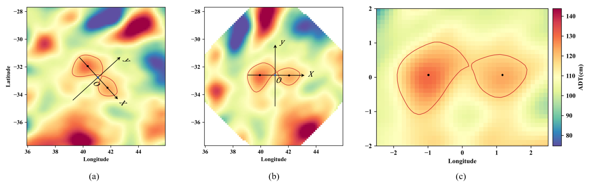
Figure 18 Schematic of the normalization process. Panel (a) shows the spatial distribution of two eddies prior to merging; panel (b) illustrates the eddy boundaries and background field after rotation; and panel (c) presents the results after scaling.

Based on the previously described two-eddy normalization procedure, the corresponding parent eddygroups were also normalized. First, the midpoint of the line connecting the centroids of the two eddies was chosen as the origin to establish the normalized coordinate system. Using the same origin as the two-eddy normalization avoids introducing relative displacement errors and preserves the spatial relationship between the parent eddygroup and the two-eddy structure throughout the normalization procedure. Next, the boundary of the parent eddygroup was then rotated by the same angle θ derived from the corresponding two-eddy event to ensure consistent orientation. Subsequently, the scaling parameter S(n) associated with the same event was applied to scale-normalize the boundary of the parent eddygroup, yielding normalized eddygroups for each event and each time point.

The area asymmetry of the interacting eddies results in an egg-shaped merged (or pre-splitting) eddy, defined by its sharp and dull poles. To accurately represent this geometry, an egg-shaped normalization was applied to the post-merging and pre-splitting states: for each frame, the major axis of the eddy was fitted and rotated to align with the x-axis, with the sharp pole toward the positive x-direction. The rotation angle β was recorded and then used for the rotation operation of the ADT background field. After orientation alignment, scale normalization was applied to the single-eddy structures that appear after merging and before splitting. Specifically, the scaling parameter S(n), derived from the two-eddy structure at the nearest time step within the same event, was used to adjust the single-eddy boundary and its corresponding background field. Since the size of the eddies involved in the same merging or splitting event typically remains relatively stable over a short period, adopting the scaling parameter determined during the two-eddy stage helps maintain scale consistency in the normalized results before and after the event, thereby facilitating meaningful comparisons of morphological characteristics across different stages. Based on this, the eddy boundaries and the ADT background were then averaged over all frames n to obtain the persistent mean morphology of the single eddy after merging and before splitting.

To assess the continuity of eddy morphology between the pre- and post-event stages, the difference in rotation angle was calculated from pre- to post-merging and from pre- to post-splitting. When the angular difference was less than $\mathit{\pi }/\mathrm{4}$, the smaller eddy before merging corresponded to the sharp pole of the merged eddy, while the larger eddy corresponded to the dull pole; similarly, after splitting, the smaller eddy corresponded to the sharp pole of the pre-splitting eddy, and the larger eddy corresponded to the dull pole. The results show that 97.73 % of merging events and 97.15 % of splitting events satisfy these relationships. This indicates that, aside from geometric changes caused directly by the approach or separation of eddies during merging or splitting, the natural evolution of eddy morphology in the pre- and post-event stages also gives rise to egg-shaped morphologies with pointed and dull poles.

The normalized results for the splitting and merging processes of eddies with different polarities are presented in Fig. 19. During the merging process, the two eddies initially manifest as nearly circular egg-shaped structures, with their common parent eddygroup exhibiting an elliptical outline. As the interaction progresses, the eddies gradually approach each other, with the boundaries on their near side converge more rapidly. Geometrically, sharp poles gradually form on the sides that approach each other, while dull poles develop on the opposite sides, thereby accentuating the egg-shaped morphology. Concurrently, the boundary of the common parent eddygroup of the two eddies also gradually develops pointed and dull poles, taking on an egg-shaped structure, with the sharp pole containing the smaller eddy and the dull pole containing the larger one. Subsequently, the two eddies transition into seed points and eventually degenerate into a single-core eddy, completing the merging process. The resultant eddy retains an egg-shaped structure in which the originally smaller eddy corresponds to the sharp pole and the larger eddy to the dull pole. Over the following days, the contrast between sharp and dull poles diminishes, and by day seven after merging (t=7), the merged eddy approaches a more regular elliptical form. The alteration in the boundaries of the eddygroup before merging and the eddy after merging shows consistency, indicating that the boundary of the merged eddy is a degeneration of the common parent eddygroup boundary of the two pre-merging eddies.

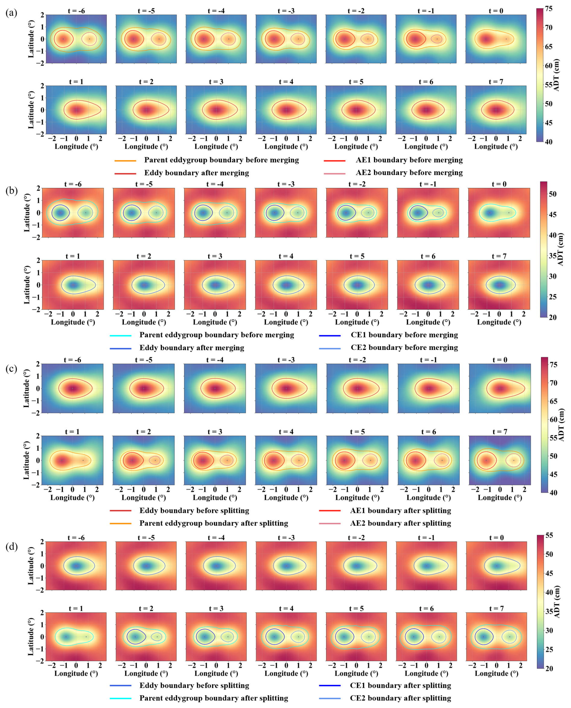
Figure 19 Normalized schematic of splitting and merging events. Panel (a) shows the normalized morphology of anticyclonic eddies before and after merging; panel (b) shows the corresponding case for cyclonic eddies; panel (c) illustrates the normalized morphology of anticyclonic eddies before and after splitting; and panel (d) shows the case for cyclonic eddies. Here, t represents the normalized time (day). AE1 and CE1 denote the larger anticyclonic and cyclonic eddies, respectively, prior to merging or after splitting.

During the splitting process, the single eddy initially exhibits an elliptical shape, which gradually develops sharp and dull poles as the event approaches, taking on an egg-shaped structure. The eddy then evolves into a multi-core structure and subsequently splits into two eddies, completing the splitting process. Notably, the two resultant eddies after splitting maintain egg-shaped morphologies, with their sharp poles oriented toward each other, while the boundary of their common parent eddygroup also exhibits an egg-shaped form. As time progresses, the egg-shaped features weaken, the separation between the two eddies increases, and the egg-shaped characteristics of the parent eddygroup gradually fade. By day seven after splitting (t=7), the two eddies tend toward a more circular shape, with the boundary of their parent eddygroup becoming elliptical. The alteration in the boundaries of the eddy before splitting and the common eddygroup after splitting shows consistency, indicating that the boundary of the pre-splitting eddy evolves into the common parent eddygroup boundary of the two post-splitting eddies.

Normalized indexes for eddy splitting and merging

During the normalized morphological evolution, the processes of eddy splitting and merging exhibit a strong form of “reciprocity.” To further investigate this behavior, the egg-shaped structure indexes proposed by (Chen et al., 2021) were introduced – the ellipticity (E) and the asymmetry (A)—to provide a quantitative description of the morphological patterns associated with eddy splitting and merging. These indexes are defined as follows:

$$\begin{array}{}\text{(1)}& {\displaystyle }& {\displaystyle }E={\displaystyle \frac{\mathrm{2}c}{a\mathrm{1}+a\mathrm{2}}},\text{(2)}& {\displaystyle }& {\displaystyle }A=\mathrm{1}-{\displaystyle \frac{a\mathrm{2}}{a\mathrm{1}}},\end{array}$$

The relevant indexes are illustrated in Fig. 20. E typically ranges between 0 and 1, where values approaching 0 correspond to shapes that are nearly circular, and values nearing 1 indicate increasingly elongated forms; in this study, E≈0.8. A varies from 0–0.8, where A=0 corresponds to a perfectly symmetric ellipse, and higher values indicate stronger asymmetry; the typical value is A≈0.1.

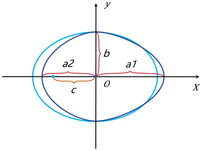
Figure 20 Schematic of elliptical and egg-shaped structure indexes. In the figure, the dark blue shape denotes an egg-shaped structure, where a1 and a2 represent the longer and shorter major semi-axes, respectively, and b represents the minor axis; the light blue curve indicates the best-fit ellipse, with c denoting its focal distance.

Building upon this framework, the study derived the morphological indexes E and A throughout the normalized processes of eddy splitting and merging. We computed the mean E and A for the two eddies (before merging or after splitting) and the values for their common eddygroup. Based on these values, time series of E and A were constructed (Fig. 21), thereby enabling a quantitative assessment and comparison of the morphological characteristics of merging and splitting events.

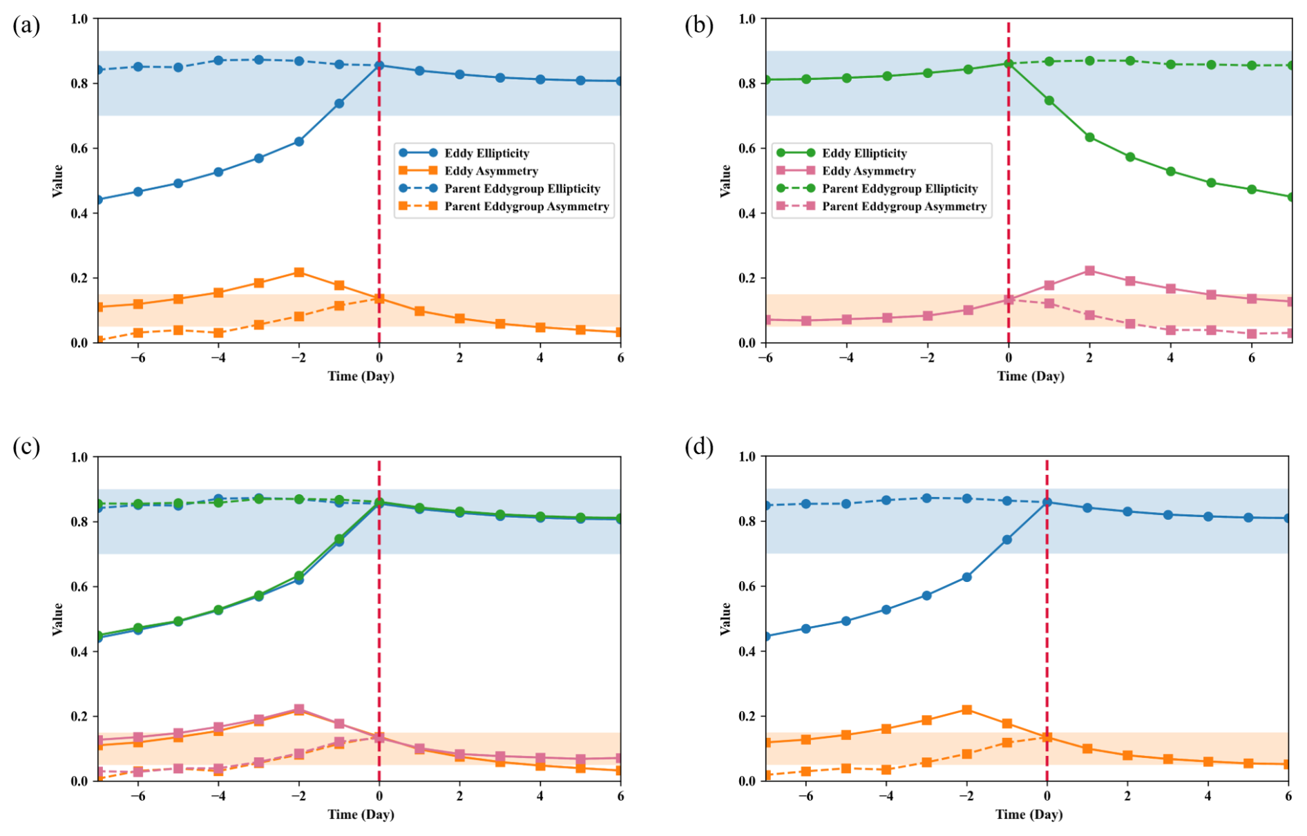
Figure 21 Schematic of parameter variations before and after eddy splitting and merging. Panels (a, b) show the time evolution of the mean ellipticity and asymmetry before and after eddy merging and splitting, respectively. Panel (c) illustrates the splitting process mirrored along the red line and plotted together with the merging process. Panel (d) presents the averaged results shown in panel (c). The vertical red dashed line marks the occurrence of splitting or merging. Dashed curves represent the mean indexes of eddies, while solid curves represent the indexes of the parent eddygroup. The blue and orange shaded regions indicate the ideal indexes ranges corresponding to egg-shaped geometries.

Figure 21a illustrates the indexes variations during the merging process. Prior to merging, the ellipticity (E, represented by dashed lines) of the two eddies increases from approximately 0.4–0.7, while their asymmetry (A, dashed lines) gradually rises from 0.1–0.2. This indicates an initial circular geometry of the eddies that progressively elongates and assumes an egg-shaped form. The common parent eddygroup shows a relatively stable E around 0.8, while A increases from 0 to about 0.15, suggesting that the parent structure begins as elliptical and gradually develops egg-shaped features. After merging, E remains stable near 0.8, whereas A decreases steadily toward zero, implying that the merged eddy maintains a relatively constant ellipticity while its shape becomes increasingly symmetric, ultimately approaching a standard ellipse. Figure 21b shows the indexes variations during the splitting process. Before splitting, the eddy maintains a nearly constant E of about 0.8, while A increases from near zero to around 0.2, indicating a transition from a symmetric elliptical shape toward an egg-shaped geometry. After splitting, the two resultant eddies exhibit a gradual decrease in A (dashed lines) from 0.2–0.1, alongside a reduction in E (dashed lines) from roughly 0.8–0.4. This suggests that the eddies retain a relatively stable degree of asymmetry but become progressively less elongated, trending toward circularity. Meanwhile, the common parent eddygroup maintains E around 0.8 while its A decreases from about 0.15 to zero, showing a transition from an egg-shaped structure to a more elliptical structure.

The variations of normalized indexes are consistent with the previously described morphological evolution. The post-merging eddy shows strong spatial and temporal continuity with the common parent eddygroup prior to merging, while the pre-splitting eddy aligns closely to the common parent eddygroup after splitting. This further underscores the crucial role of eddygroups in splitting and merging events: the boundary of the pre-merging parent eddygroup of the two eddies degenerates into the boundary of the merged eddy, and the boundary of the pre-splitting eddy evolves into the boundary of the post-splitting parent eddygroup of the two resultant eddies.

By employing the time of splitting as a symmetry axis, the indexes variations during splitting were mirrored and aligned with those of merging (Fig. 21c). The results show a high degree of consistency in E between the merging process and its inverse, the splitting process, with A also demonstrating concordance. This demonstrates that, in normalized coordinates, eddy merging and splitting can be regarded as reciprocal morphological processes. Furthermore, by treating merging and splitting as the forward and reverse phases of the same process, the overall indexes variations can be depicted as shown in Fig. 21d. And the figure illustrates that when the eddy splitting and merging events occur, the A of the eddygroup reaches its maximum.

4 Data availability

The dataset can be accessed at https://doi.org/10.12237/casearth.20250026 (Tian et al., 2025). The dataset is saved in JSON format, ensuring straightforward compatibility with common scientific programming languages like Python, MATLAB, and R. For detailed data, please refer to Appendix A or download the Dataset User Guide file from the data website.

5 Conclusions and future work

This research improved the identification algorithm for eddies and eddygroups using ADT data spanning from 1993–2023, and further separated the construction of multi-level eddytrees as a post-processing step. By applying an area-based ranking approach for eddygroups to establish hierarchical relationships from the outside inward, the overall computational efficiency of the algorithm was enhanced by roughly a factor of eleven compared with existing methods. For the tracking of eddy splitting and merging, a Lagrangian particle-drift approach is introduced to establish segments of eddies between consecutive days, thereby avoiding dependence on subjective thresholds, and ultimately achieving eddygraph tracking of splitting and merging events.

Based on the improved algorithm, two categories of data products were produced: (1) a global dataset of mesoscale eddy and eddygroup identifications from 1993–2023, including the associated multi-level eddytree topology; and (2) a trajectory dataset of eddy splitting and merging events over the same period.

Analysis of the dataset reveals that eddies and eddygroups are more active along oceanic margins and in mid- to high-latitude regions, while they are relatively scarce in the equatorial zone. Using the polarity of the root node to characterize eddytree polarity, it can be seen that: anticyclonic eddytrees predominate year-round in regions dominated by strong western boundary currents; in regions of strong warm–cold current confluence, a distinct boundary between cyclonic and anticyclonic eddytrees emerges, forming a dipole-like eddytree structure, with the boundary extending from the circulation into the ocean interior and gradually weakens; island topography in the open ocean obstructs the flow and gives rise to von Kármán-type vortex-street structures in the wake region of the islands; and the boundaries between eddytree polarities are generally coincide with stable large-scale ocean circulation. Statistics of event frequency further indicate that splitting and merging events occur most frequently in dynamically unstable regions. Merging events occur at approximately three times the frequency of splitting events. To further investigate the morphological evolution of splitting and merging, ellipticity (E) and asymmetry (A) were applied within a rotated and scale-normalized eddy coordinate system. The results show that during merging, two eddies transition from near-circular forms into egg-shaped structures, and after merging, the egg-shaped structures gradually transition into elliptical forms. During splitting, the eddy evolves from an elliptical form into an egg-shaped structure, while the egg-shaped features of the two splitting eddies weaken over time and gradually approach circular forms. Eddygroups play a key role in these processes: the boundary of the pre-merging parent eddygroup of the two eddies degenerates into the boundary of the merged eddy, whereas the boundary of the pre-splitting eddy evolves into the boundary of the post-splitting parent eddygroup of the two resultant eddies. By mirroring the time axis, it becomes evident that merging and splitting processes exhibit nearly reciprocal features in normalized morphological space: the evolution of E is highly consistent between the two, and A also shows strong correspondence.

However, several topics remain for future work. First, this study provides a preliminary definition of the polarity of eddygroups and eddytrees; however, their physical oceanographic significance still requires further investigation. The inclusion relationships between eddygroups and eddies of different polarities, along with the interaction mechanisms of dipoles within eddygroups, also remain to be explored. In addition, this study only presents a preliminary exploration of the relationship between eddytree structures and large-scale ocean circulation. In bounded oceanic regions with limited spatial extent, most sea surface height (SSH) contours are theoretically closed. With ongoing advancements in satellite altimetry, it is anticipated that SSH-derived closed contours will encompass broader areas of the global ocean. The ocean current field data we are dealing with is filled with thousands of mesoscale, submesoscale, and even smaller-scale oceanic phenomena. How to more efficiently analyze this seemingly chaotic, integrated flow field and establish a multi-scale hierarchical spatiotemporal structure of the flow field is essential. Compared with gridded representations of ocean currents, such as maps of ADT, the eddytree framework may provide a hierarchical vectorized representation of ocean current structures – an approach whose application potential has yet to be explored. Second, this study develops a global dataset of eddy splitting and merging events, but the variations in their spatial distribution across different ocean regions need more detailed examination. Additionally, the research primarily concentrates on the morphological characteristics of the eddy splitting and merging processes involving two eddies, while whose involving three or more eddies remain to be further explored. And their dynamical and kinematic mechanisms still need further investigation. And the tracking of splitting and merging events in this study is limited to the terminal nodes of the eddytree (eddygroups and eddies). However, as a hierarchical structure extending up to 60–70 levels in some regions (e.g., the Kuroshio Current and its extensions) and exhibiting amplitudes reaching 40 cm, it is possible to further simplify the framework by extracting its skeleton. The dynamical processes represented by this skeleton warrant further exploration of their morphological, kinematic, and dynamic regularities. Third, the hierarchical structure revealed between eddygroups and eddies indicates that within the eddytree, the relationships both among eddygroups at different levels and between eddygroups and eddies exhibit a fractal-like self-similarity. This observation raises the possibility that analogous hierarchical structures may also exist between mesoscale eddies and submesoscale ocean features, thereby offering a new perspective for the study of submesoscale processes. Fourth, oceanic eddies are inherently three-dimensional structures, yet the present investigation of global splitting and merging patterns is restricted to two-dimensional surface data. Future research will investigate the dynamic patterns associated with three-dimensional eddy splitting and merging processes.

Appendix A: Detailed description of the dataset

This study produced datasets spanning the period from 1993–2023 (Tian et al., 2025), comprising the identification of eddies and eddygroups along with their topological relationships, as well as the tracking of eddy splitting and merging. Furthermore, the dataset incorporates normalized selected typical cases of eddy splitting and merging.

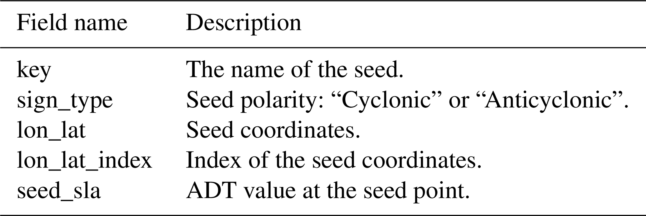
The identification data are stored on an annual basis, with each day recorded as a separate JSON file. Each JSON file mainly contains three modules: eddies, eddygroups, and seed points. Tables A1–A3 provide detailed parameters and their corresponding descriptions for the eddy, eddygroup, and seed point modules, respectively. In addition, elements in these three modules are further classified according to specific conditions, such as whether a seed point is independent or whether it is included only within an eddygroup. However, the main analyses remain focused on the three primary modules described above.

The tracking data are stored annually in JSON files, where each entry in a JSON file represents a single tracking trajectory. Each trajectory is composed of multiple branches, and each branch contains several items. The final item of each branch contains four specific keys: “begin”, which denotes that the branch is either newly generated or originates from the splitting or merging of other branches; “end”, which signifies that the branch terminates or undergoes splitting or merging into particular eddies or eddygroups; “merge”, which, if non-empty, indicates that the branch ultimately experiences a merging event; and “split”, which, if non-empty, indicates that the branch ultimately undergoes a splitting event. The remaining items within a branch are structured as a list that includes the name (such as seed point, eddy, or multi-core eddy), the spatial coordinates [longitude, latitude], and the associated date.

The typical splitting and merging event data are stored in two JSON files, each further categorized into cyclonic and anticyclonic events. Within the merging file, each event is characterized by three keys: “before1” and “before2”, which denote the two eddies prior to merging, and “after”, which represents the resultant merged eddy. Conversely, in the splitting file, each event includes the key “before”, indicating the eddy prior to splitting, alongside “after1” and “after2”, which correspond to the two eddies formed post-splitting. Under each key, information for the corresponding eddy over seven consecutive days is stored, including the date, name, centroid coordinates, effective boundary, parent eddygroup, and parent eddygroup boundary details.

Table A1 Stored information and related descriptions for each element in the eddy module.

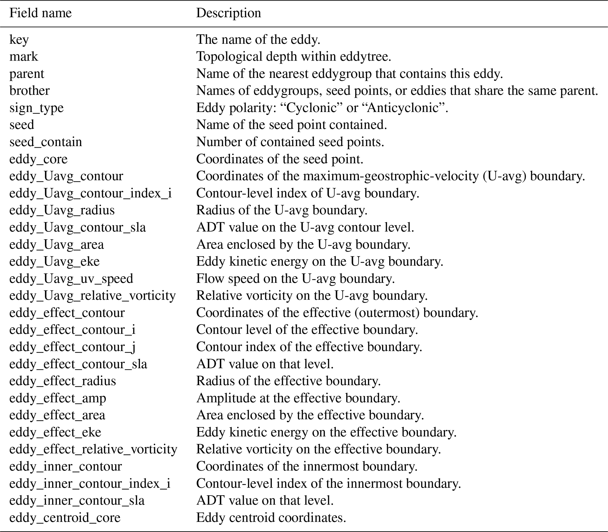
Table A2 Stored information and related descriptions for each element in the eddygroup module.

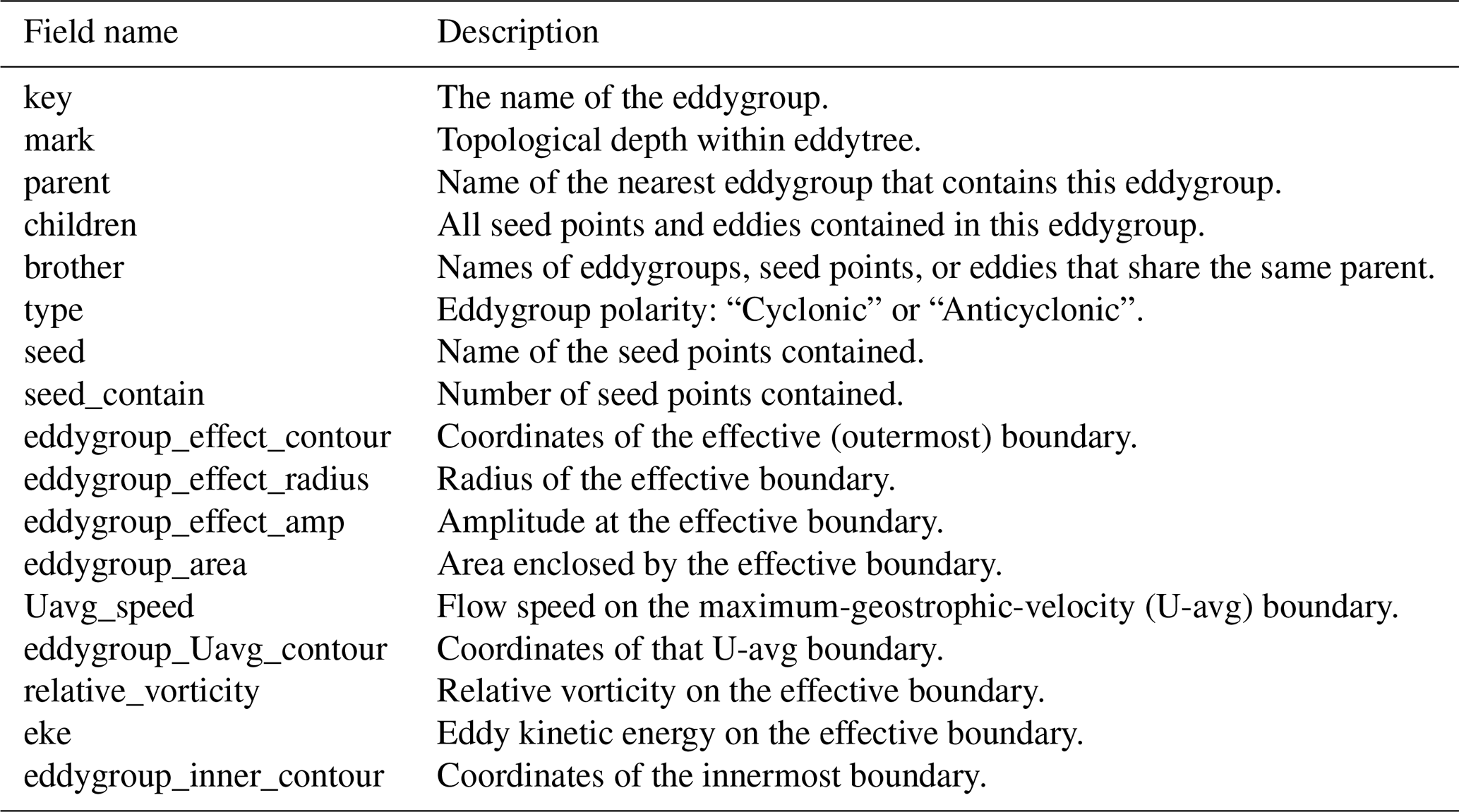
Table A3 Stored information and related descriptions for each element in the seed point module.