GRACE and GRACE-FO mascons for ocean dynamic applications

A new series of mascons are made from GRACE and GRACE-FO data, specifically designed for use by oceanographers interested in studying variations in ocean mass transport and circulation. This series has pre-removed those changes in ocean mass distribution caused by barystatic gravity, rotation, and deformation (GRD) signals, as well as the non-oceanographic signals caused by four major oceanic earthquakes, neither of which impact circulation. Subtle changes in the processing and regularization schemes also help reduce the visibility of instrument/orbital errors in the ocean signal, particularly in the Arctic and near the sites of the removed earthquakes. The primary benefit of this data set is increased ease of use for researchers interested in ocean dynamics, as the product is designed to be used “off the shelf” with no additional corrections required, even by those less familiar with GRACE data usage. The complete dataset is available at https://doi.org/10.18738/T8/3VUPEW (Pie et al., 2025).

1 Introduction

Since its launch in 2002, the Gravity Recovery and Climate Experiment (GRACE) and (since 2018) its Follow-On successor (GRACE-FO) have provided a unique view of the water mass exchange between the oceans, land, and cryosphere (Tapley et al., 2019). While hundreds of articles have used GRACE and GRACE-FO data (hereafter GRACE/FO) for studying important aspects of land hydrology (e.g.: Rodell and Reager, 2023) and the cryosphere (e.g.: Ciracì et al., 2020; Velicogna et al., 2020), the data can also be used for studying mass transport within the ocean (e.g., see Wahr et al., 1998 for the theoretical basis).

Some examples of ocean-focused studies include combining the mean geoid from GRACE with satellite altimetry to capture the surface geostrophic circulation (Tapley et al., 2003; Feng et al., 2013), quantifying seasonal and interannual mass exchanges in the North Pacific (Bingham and Hughes, 2006; Chambers and Willis, 2008; Song and Zlotnicki, 2008; Chambers, 2011; Cheng et al., 2013), and investigating high frequency mass exchanges in the South Pacific (Boening et al., 2012). The data have also been used to study interannual large-scale mass exchanges between the Pacific and Indo–Atlantic ocean basins (Chambers and Willis, 2009), as well as transports of the Antarctic Circumpolar Current (Zlotnicki et al., 2007; Bergmann and Dobslaw, 2012; Makowski et al., 2015), Atlantic Meridional Overturning Circulation (Landerer et al., 2015), and Antarctic Bottom Water (Mazloff and Boening, 2016; Jeffree et al., 2024).

These studies all used either gridded spherical harmonic data or gridded ocean mass concentration (mascon) blocks (Save et al., 2012, 2016; Watkins et al., 2015; Wiese et al., 2016; Loomis et al., 2019) that contain both oceanographic and other geodetic signals unrelated to ocean dynamics, such as gravity, rotation, and deformation (GRD) signals (e.g., Farrell and Clark, 1976), global atmospheric pressure variations (e.g., Chambers and Schröter, 2011), as well as leakage from larger hydrology and ice sheet variations. Because GRD and leakage are largest near land and are significantly larger than ocean signals, the general recommendation has been to ignore GRACE/FO ocean grids within 300 km of land (e.g., Chambers, 2006; Chambers and Schröter, 2011) where these geodetic and leakage signals tend to be significantly larger than ocean signals. Even more problematic are large trends in the Indian Ocean and off the coast of Japan due to large earthquakes (Chao and Liau, 2019; Bonin et al., 2026). While most oceanographic studies utilizing GRACE/FO data have attempted to mitigate large geodetic signals by examining areas away from land and removing a global ocean monthly average (to remove the globally uniform, or barystatic, portion of the signal), others have not. These non-oceanographic signals likely contributed to some increased error in the results.

To improve the utility of GRACE/FO data for oceanographic applications, we have created a set of gridded mascons where the largest known non-oceanographic geodetic signals have been explicitly removed, such that the remaining ocean mass variability is predominantly driven by ocean circulation changes. To accomplish this, we utilize the Center for Space Research release 6.2 (CSR RL06.2) mascon processing stream (Save et al., 2016; Save, 2020a) with alterations. The CSR RL06.2 processing stream already removes a model for glacial isostatic adjustment, restores a geocenter (degree 1) estimate, and replaces C₂₀ and C₃₀ with values based on satellite laser ranging (see details in Sect. 2).

For the dynamic ocean (DO) mascons that we have created (designated as the CSR RL06.2DO series), we modify the geocenter correction slightly and remove the barystatic-GRD signal for each month that results from the redistribution of mass between land and ocean (e.g., Tamisiea et al., 2010). We also remove solid earth mass change from four large oceanic earthquakes (Bonin et al., 2026) and we remove the global atmospheric pressure average over the ocean (Chambers and Schröter, 2011). The monthly barystatic-GRD signal is provided separately. Likewise, the earthquake model used is provided so users can add it back and apply their own earthquake model. However, as discussed in Bonin et al. (2026), the earthquake signals as they appear in different mascon solutions vary considerably due to center-specific processing choices. The model we include is specific to the CSR processing and should not be used to remove earthquake signals from the JPL or GSFC mascons, or from any spherical harmonic solutions.

Because of these changes, the CSR RL06.2DO mascons are not appropriate for comparisons with ocean bottom pressure gauges, as they omit the pressure impact of the atmosphere and barystatic-GRD signals, which are measurable by pressure recorders. Nor are they intended to be used for global sea level budget studies, as the sea-surface height changes associated with GRD are also present in satellite altimetry (Ponte et al., 2018) but have been removed from the DO mascons. We would recommend using the standard mascons for most sea level budget studies unless users are trying to separate GRD and dynamic ocean contributions. The DO mascons are designed primarily for ocean dynamic applications, such as computing bottom currents, mass redistribution due to circulation changes, or oceanic sources of polar motion. They also should be more useful for assimilation into oceanographic models, which typically do not model barystatic-GRD or global atmospheric pressure changes.

Section 2 will describe the specific methods and data used in the creation of the CSR RL06.2DO data, including descriptions of: the mascon processing scheme and how it differs from RL06.2 (Sect. 2.1); the changes to the regularization scheme and how those impact the land/ocean mask (Sect. 2.2); the removed earthquake model (Sect. 2.3); and the removed barystatic-GRD model (Sect. 2.4). Section 3 will describe the differences between the standard CSR RL06.3 and CSR RL06.2DO mascons, and the Estimating the Circulation and Climate of the Ocean (ECCOv4r4) (ECCO Consortium et al., 2021a, b) constrained state estimate based on the MIT general circulation model (MITgcm). There we show a reduction in variance by removing the barystatic-GRD and earthquake signals and showing significant improvement in several coastal areas. Section 4 will conclude by discussing how these new DO mascons can be utilized in oceanographic applications without having to ignore (or approximate) non-oceanographic geodetic signals.

2 Data and methods

The standard CSR GRACE/FO mascon series (Save et al., 2016; Save, 2020a) are gridded products available over the entire globe, both land and ocean. Each of the equal-area 40 962 hexagonal (and 12 pentagonal) mascons are roughly 120 km in diameter and are subdivided into “land” and “ocean” sections when located along coastlines. Though the data is released on a uniform $\mathrm{1}/\mathrm{4}$° grid, the true resolution of the data is ∼ 200–300 km, because the regularization uses information with ∼ 200 km resolution and the mascon signal is still limited by the fundamental ∼ 300 km spatial resolution defined by GRACE/FO's orbit altitude. The regularization better reduces the anisotropic stripe-pattern errors typical of the GRACE/FO solutions. It also more precisely localizes large land/ice signals into land mascons, thus reducing the spread of those land-based signals into ocean areas which naturally contain much less mass variability (e.g., Watkins et al., 2015; Save et al., 2016).

The dynamic ocean mascons are created using a process (Sect. 2.1) that is very closely related to the CSR RL06.2/RL06.3 (Save et al., 2016; Save, 2020b) mascon processing. (RL06.2 and RL06.3 do not differ in their general processing methods, though RL06.3 ingests different accelerometer data than RL06.2 and RL06.2DO in the later months). The estimation of the RL06.2 mascons is performed with respect to a background model that aims at representing most of the known time variable gravity signals: annual and semi-annual signals globally, plus trends in the icy regions of Greenland and Antarctica. This results in minimal peak shaving of these large signals during regularization, since the amplitude of the correction signal is roughly the same size over the entire land region (Save et al., 2012). For the estimation of the RL06.2DO mascons, we modified the estimation background model so that it would also include mass signals from major earthquakes and a preliminary approximation of the barystatic-GRD effect associated with the linear trend of modern-day ice mass loss as measured by GRACE/FO. We also altered the sequence of when we apply the ellipsoidal correction relative to other corrections (e.g., the replacement of C₂₀/C₃₀). All these changes are described in Sect. 2.1.

Following the changes in the RL06.2DO estimation background, we modified the regularizing constraints applied in the CSR mascons' estimation, to reduce the estimation error in regions near large earthquake signals and to better localize the ocean signals and to reduce the impact of instrument and orbit errors in the Arctic Ocean. The Arctic constraint changes resulted in a slight change of the standard CSR land/ocean mask definition, such that the ocean-only DO mascon series excludes the Arctic islands of Franz Josef Land, which contain land areas experiencing measurable grounded-ice mass loss, but were treated as purely “ocean” mascons in the standard CSR mascon products. This is described in detail in Sect. 2.2.

Since the primary objective for the DO mascon is to remove non-oceanographic signals over the ocean, we also remove three new signals during or after the creation of the DO mascons. First, during the pre-processing, we model and remove the impact of four major earthquakes. Our earthquake model includes the very large 2004 Andaman-Sumatra earthquake (magnitude 9.2) in the Indian Ocean and the 2011 Tōhoku, Japan quake (magnitude 9.0), both of which are easily visible in the current GRACE/FO ocean mascons. This removes the most visible solid earth signal in the ocean mascons, though we note that residual signal from these earthquakes and signal from other quakes remains in the DO mascons, as do other types of deeper solid earth mass signals (Mandea et al., 2015; Gouranton et al., 2025). By removing these few quakes by a simple model, as described in Sect. 2.3, we remove a large fraction of the ocean-area signal that is not related to oceanographic processes.

Second, as a new post-processing step, we remove the precise monthly GRD pattern that results from mass exchange between the land and ocean, as computed from the estimated land DO mascons themselves (Sect. 2.4). While mass in the ocean is increasing as ice sheets melt (Chambers et al., 2017; Cazenave et al., 2019), the barystatic-GRD is a purely geodetic signal and has no direct relationship to physical processes in the ocean driven by wind and/or buoyancy fluxes. We also remove the monthly average over the global oceans of the restored GAD (Sect. 2.4), as this is caused by monthly-varying uniform atmospheric pressure changes over the ocean (Chambers and Schröter, 2011). Such a uniform pressure change will not cause any ocean dynamical signal.

Overall, the signal content of the DO mascons (over ocean grids only) can be approximately related to the original RL06.2 mascons by:

$$\begin{array}{}\text{(1)}& \begin{array}{rl}\text{RL06.2DO}(x,y,t)& \approx \text{RL06.2}(x,y,t)-\text{GRD}(x,y,t)\\ & -\text{EQ}(x,y,t)-{\mathrm{GAD}}_{\mathrm{avg}}\left(t\right)\end{array}\end{array}$$

where (x,y) are the spatial location, t is time, GRD refers to the barystatic-GRD mass estimate (released with the product), EQ refers to the earthquake mass estimate (released with the product), and GAD_avg is the monthly spatial average over the oceans of the standard GAD product (Dobslaw et al., 2017) released on the CSR mascon grid (available at https://download.csr.utexas.edu/outgoing/grace/RL0603_mascons/CSR_GRACE_GRACE-FO_RL0603_Mascons_GAD-component.nc, last access: 3 November 2025). The equation is not exact due to changes in regularization weights, masking, geocenter updates, and implementation of the ellipsoid correction (Sect. 2.1). The globally-averaged RMS error (RMSE) relative to the real DO mascons (weighted by latitude) is 0.49 cm. Much of that is due to large differences near the modelled earthquakes (RMSE > 15 cm; see Sect. 2.3) and in the Arctic near Franz Josef Land (RMSE > 4 cm; see Sect. 2.2). Coastal RMSE are typically 0.5–2.0 cm. Open ocean (exclusive of the Arctic and earthquake zones) differences between the actual DO mascons and the approximation given by Eq. (1) are 0.35 cm water height on average.

Like all other CSR GRACE/FO mascon products, mass changes estimated in the DO mascons are presented in units of equivalent water height, relative to the 2004–2009 DO mascon mean. A saltwater estimate of density (1025 kg m⁻³) is used to compute the height (in cm) of water which, spread over a given area, which would equate to the mass anomaly observed by GRACE/FO.

2.1 Alterations to mascon estimation background model and processing

All the background models from the GRACE/FO CSR Level-2 RL06 Processing Standards documentation (Save, 2020a) are already accounted for in the spherical harmonics normal equations of the official CSR RL06.2 Level-2 solutions, from which the mascon normal equations are derived. In particular, these background models include the GOT4.8 ocean tide model and the non-tidal atmospheric and ocean de-aliasing (AOD) model, AOD1B RL06 (Dobslaw et al., 2017). To further minimize estimation errors and peak-shaving due to regularization, CSR mascons are estimated with respect to an a priori background model which also includes most of the large known gravity signals. The background model used for the CSR RL06.2 mascons includes trends over large ice-covered regions, annual and semi-annual signals globally (both estimated from RL05 versions of GRACE/FO), and a glacial isostatic adjustment (GIA) based on the ICE-6G_D GIA model (Peltier et al., 2017). This estimation background model (excluding GIA contribution) is restored prior to release.

The background model used for the estimation of the RL06.2DO mascons builds on the one used for RL06.2 mascons by adding an earthquake model and a preliminary barystatic-GRD model that complements the expected ice mass trend. The earthquake model, described in Sect. 2.3, was derived from the standard RL06.2 CSR mascons, in an iterative process. It accounts for the signals from the large earthquakes in Andaman Bay and near Japan over the GRACE/FO period. Because RL06.2 and RL06.3 do not model the large amplitude of these earthquake signals, incorporating the huge (50–100 cm) jump caused by the co-seismic solid earth signal of the earthquakes into the mascons requires the use of extremely loose regional constraints. If the constraints were not left loose enough, the earthquake signal leaked into other neighbouring mascons, corrupting the ocean and hydrology signals. However, relaxing the constraints allowed more than the desired earthquake signal in; it also increased the month-to-month noise in near-earthquake mascons by an order of magnitude over other ocean mascons (Bonin et al., 2026). By removing most of the earthquake signal as a pre-processing background model, we have largely remedied this in the DO mascons, resulting in a better solution with lower month-to-month noise around the major earthquakes.

Second, the large mass loss from ice-covered regions corresponds to a barystatic-GRD ocean mass trend which is very apparent in RL06.2 ocean mascons, particularly near the coasts of Greenland and Antarctica. In the DO mascons, a preliminary barystatic-GRD model is added to the background, computed as the response to the long-term linear ice mass trend estimate already included in the RL06.2 background model. This calculation is less complete than our final barystatic-GRD estimate, described in Sect. 2.4, which we remove from the DO mascons during post-processing, since it is only driven by an estimate of ice mass trend. Removing the majority of this known signal helps during mascon estimation because the tighter ocean constraints may not allow for the GRD signal to adjust into the ocean regions correctly. We found that its primary impact was to enable larger ocean mass trend estimates in the immediate vicinity of the ice sheets, where the GRD signal is the largest. This preliminary GRD model is restored at the end of the estimation process.

In addition to these major changes in the background model, we have also made more subtle changes to the CSR mascon processing scheme. In the standard RL06.2 (and RL06.3) CSR mascon processing, an ellipsoid correction accounting for the true shape of the Earth (Ditmar, 2018) is applied to the mascon estimates before other corrections are applied. The ellipsoid-corrected RL06.2 mascons estimates are then altered so that the contributions of the C₂₀ and C₃₀ terms (converted to water layer grids) are replaced with values based on satellite laser ranging (SLR) using GRACE TN-14 (Loomis et al., 2020), and a geocenter degree 1 estimate is added using GRACE TN-13 (Sun et al., 2016b). Finally, a GIA model (ICE6G-D; Peltier et al., 2017) is removed from the mascon grids and the standard CSR Level-2 GAD (which represents the AOD1B model over the oceans, Dobslaw et al., 2017) is added back, leading to the fully-corrected RL06.2 mascons.

When creating the DO mascon series, we revised the order of corrections applied to the standard CSR mascons. The replacement of C₂₀/C₃₀, the addition of the geocenter terms, and the removal of GIA geopotential are now done prior to the ellipsoidal correction, because these terms are expressed on a spherical Earth and should not be applied directly to a field expressed on an ellipsoid Earth. Also, as specified in Ditmar (2018), the ellipsoid correction applies to the 2-D surface mass anomalies only and not to the solid Earth mass transport, which occurs much deeper (tens to hundreds of km deep). Therefore, it is necessary to remove such signals from the mascons prior to applying the ellipsoid correction. Aside from their order with respect to the ellipsoidal correction, corrections of the C₂₀ and C₃₀ terms and GIA were kept the same as those applied to the RL06.2 mascons.

Just as there is a different version of TN-13 for each SDS spherical harmonic distribution, the mascons should have a degree 1 contribution that is consistent with the rest of its mass change distribution, a strategy currently used in the JPL mascons. As we want to estimate and remove a barystatic-GRD estimate, it is easy to simultaneously estimate the degree 1 contribution, similar to Sun et al. (2016b) and Swenson et al. (2008). An intermediary set of mascons (after the ellipsoidal correction), used in the barystatic-GRD calculation, includes the TN-13 correction designed for CSR's L2 spherical harmonic solution. After the new degree 1 contribution is estimated, it replaces the TN-13 values, and the ellipsoidal correction is recalculated.

2.2 Alteration of regularization constraints

All CSR mascons are regularized (Save et al., 2012, 2016), with constraints that vary in different areas of the world, and even at different times of the year. Regularizing constraints are represented as sigmas (standard deviations) because they are connected to the expected variance of the signal in the region, such that lower values of sigma mean constraints that tightly limit the estimate, and higher sigma values mean looser constraints that allow the estimate more flexibility to adjust and hold larger signal variability. Sigma values over land are higher than those in the ocean (typical land sigmas are ∼ 10–30 cm, while ocean sigmas are ∼ 3–5 cm), as land/ice variability is expected to be higher than ocean signal variability.

The first major regularization constraint change in the DO mascons was to tighten the very loose constraints in Andaman Bay and near Japan back to “normal” ocean constraint levels. While RL06.2 used very large regularizing sigmas in those localized regions to let in the earthquake signals and not smear them over large spatial scales, estimating the DO mascons with respect to a background model that already includes these large signals eliminates the need for such an accommodation in the constraints. Therefore, the RL06.2DO ocean mascon constraints near the earthquake epicenters are defined as they are in the rest of the global ocean, with typical values between 3–5 cm (since the regularization does not have to adjust the large earthquake signals anymore).

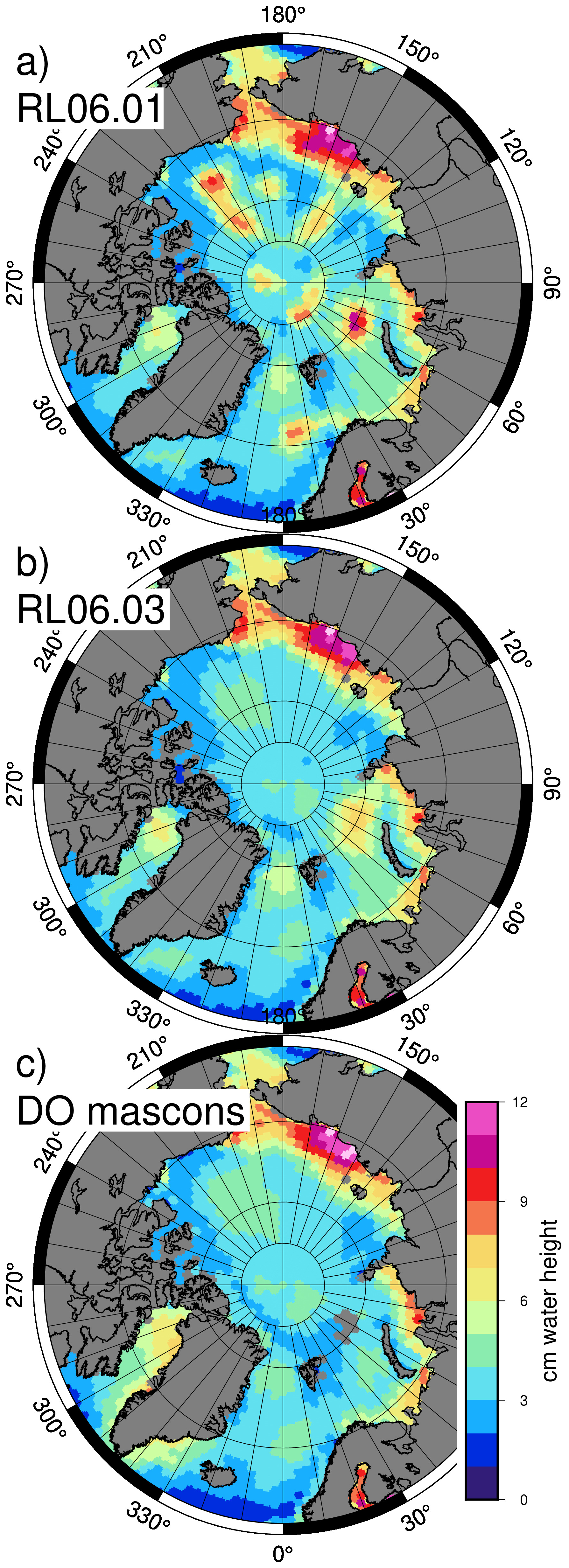
Figure 1 Signal RMS over the ocean of (a) CSR RL06.1 mascons, (b) CSR RL06.3 mascons, and (c) the dynamic ocean mascons with barystatic-GRD, EQ, and GAD_avg restored.

The second major change in the definition of the regularization constraint was implemented over the Arctic Ocean. In the previous CSR mascons, up through the RL06.1 release, the Arctic ocean mascon constraints were in part defined by a 12-month climatology based on the older RL05 CSR mascons (Fig. A1). During early research in creating the DO mascons, we determined that the residual north/south stripe errors present in this climatology resulted in physically unrealistic striations in the Arctic Ocean (Fig. 1a), which were very unlikely to represent real ocean signal. These errors are largest near the poles and were particularly noticeable over the Arctic Ocean. As a result of our investigations, in CSR mascon series RL06.2 and RL06.3, the constraint definition was changed over the Arctic Ocean to exclude this GRACE-based climatology, using only a 12-month climatology defined by the GAD values from the AOD1B product, which cannot contain GRACE-style stripe errors. A lower-bound for the constraint sigmas was set to 3 cm (to prevent the GAD series from understating real signal) and an upper-bound set to 5 cm. This removed the unrealistic Arctic striations, while still allowing the constraints to vary realistically and seasonally (Figs. 1b and A2).

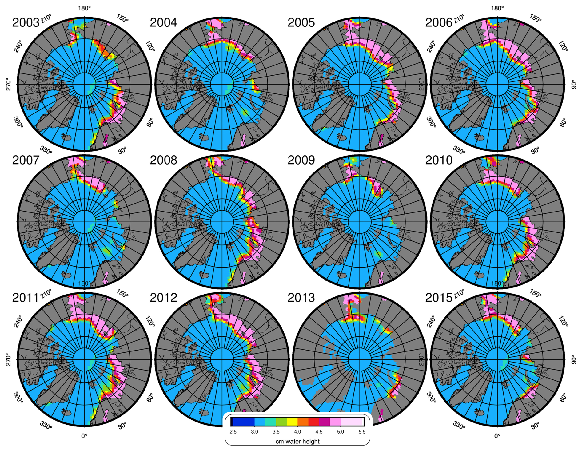
Figure 2 Examples of variability in constraint sigmas for RL06.2DO: first twelve February months. Unlike the RL06.2 constraints, the DO sigmas are not identical per month over the years.

There is substantial variation in the actual Arctic Ocean signal which is not captured by a simple climatology (e.g., Fig. 2). In months when the real signal is substantially smaller than the climatological expectation, the RL06.3-style regularization constraints may be too loose, such that too much noise enters the ocean. For the DO mascons, we wished to tighten the constraints during “quiet” months to improve the visibility of ocean circulation (which is of relatively small magnitude). To accomplish this, we defined the value of the constraint to be the minimum of two values: (1) the absolute value of the specific month's local GAD value, or (2) the GAD climatological value for that calendar month. On top of this, we applied the same 3–5 cm bound on the constraint sigmas in all Arctic mascons, to eliminate cases where there would either be too little or too much constraint flexibility. The result is a set of constraints which varies uniquely for each month, rather than following a strict climatology (Figs. 2 and A3). Overall, this tends to tighten the constraints along the coasts of northern Eurasia. It does not notably alter the constraints in areas away from the coastlines.

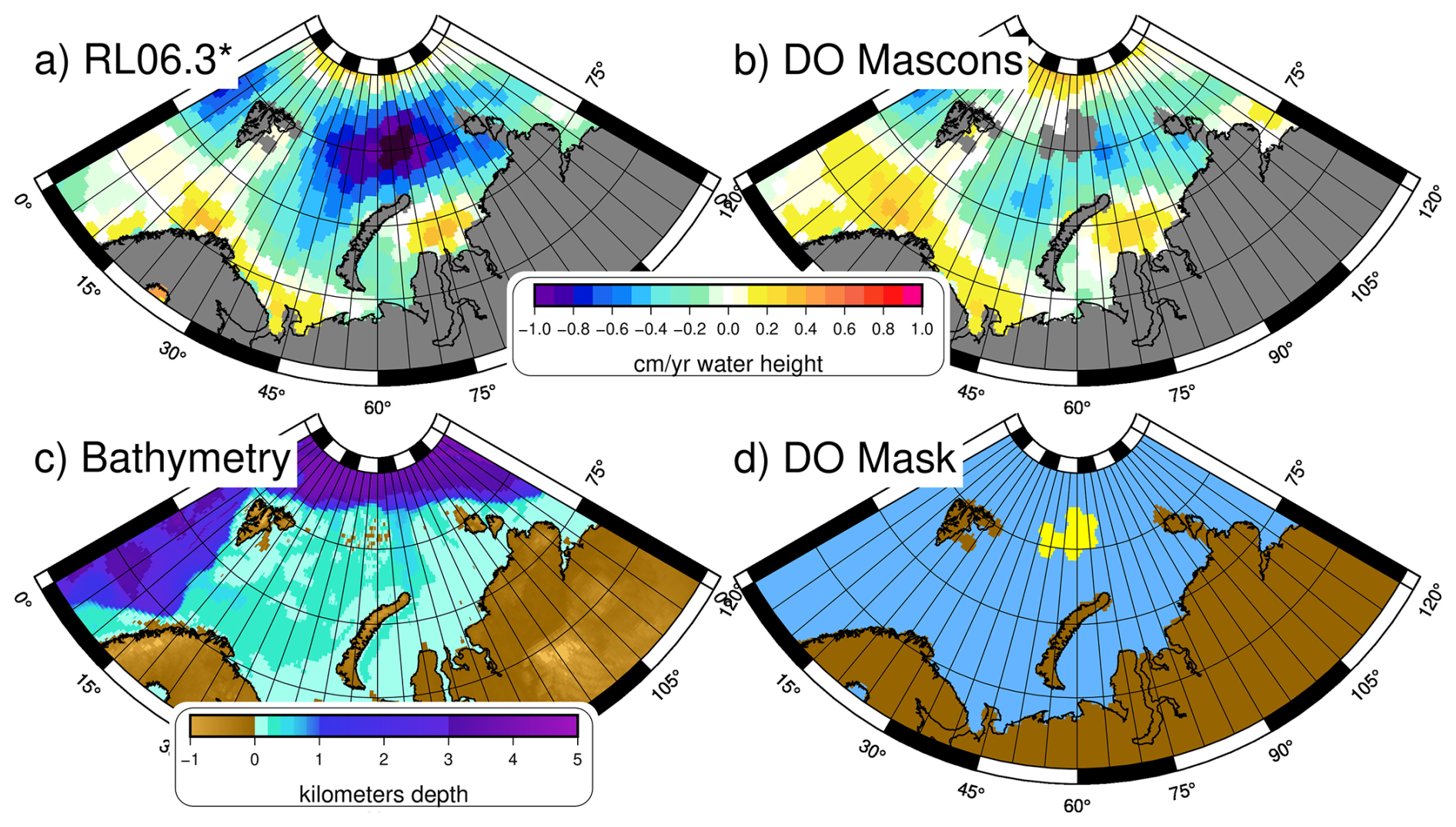
Figure 3 Trends of (a) the CSR RL06.3 mascons, after an appropriate GRD series and GAD_avg have been removed, and (b) the DO mascons. The ETOPO1 bathymetry (c) shows the location of Franz Josef Land, which is masked as “land” (yellow) in the DO mascons (d).

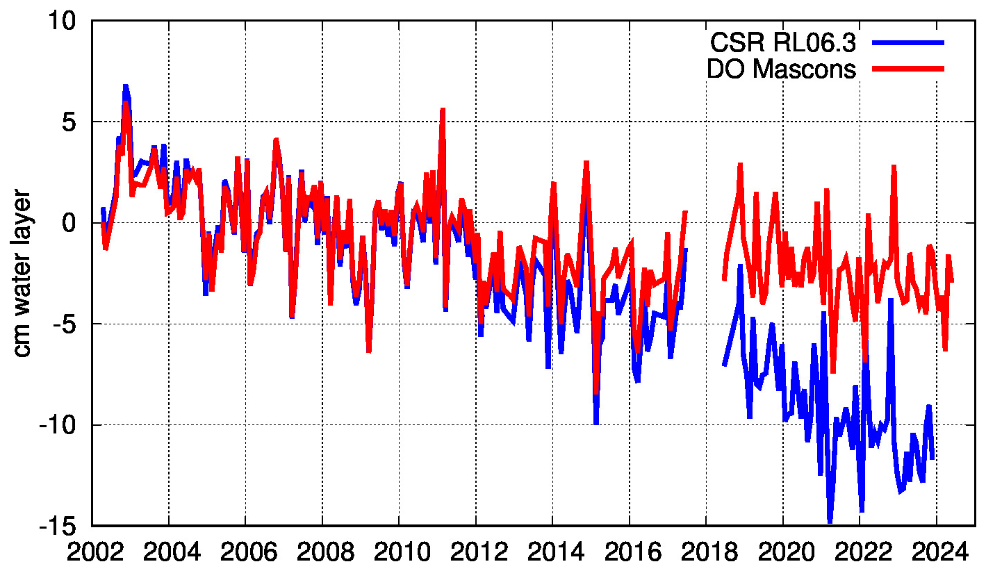
Figure 4 Average mass loss near Franz Josef Land over DO-defined ocean mascons only (longitudes 78–84° N and latitudes 35–80° E) for the DO series vs the CSR RL06.3 mascons (minus GRD and GAD_avg). Both series omit values in the newly-defined “land” mascons over Franz Josef Land.

The ocean variability which results from these constraint changes (Fig. 1c) is still quite close to that of the RL06.3 mascons (Fig. 1b). However, during our exploratory work into defining these new constraints, we noted that after removing the GRACE-based climatology from the Arctic Ocean constraints, a region of extremely high variability remained around 60° E (Fig. 1b). The majority of this signal is caused by a near-linear trend (Fig. 3a), which is considerably larger than trends elsewhere in the Arctic Ocean and does not have a known oceanographic explanation. This mass-losing region of the Arctic Ocean lies on top of Franz Josef Land (Fig. 3c), an icy archipelago that is 85 % glaciated and strongly suspected to be a place of land ice mass loss (Jacob et al., 2012; Zheng et al., 2018; Schmidt et al., 2025). In all former GRACE/FO mascons (including CSR RL06.3 and the JPL and GSFC mascons), mascons overlaying Franz Josef Land have been officially considered “ocean”, rather than “land”, since they are more ocean than land, area-wise. In the CSR methodology, this means that the eight mascons covering these islands (yellow grids in Fig. 3d) had been assigned the very tight constraints applied to ocean mascons. However, if these areas are truly losing land-ice mass at a large rate, then by tightly constraining the signal, that mass loss will not be able to be contained in the local area but will instead leak out into the broader ocean area, which is what we observe in RL06.3 (Fig. 3a).

In the DO mascons, we instead denote these eight mascons as “land”, assigning them looser constraints based on the normal CSR land constraint definition. The “land” constraint sigmas over these island mascons typically vary between 4–8 cm over the lifetime of the mission. Redefining these eight mascons as “land” greatly reduced the trend (Fig. 3b) and RMS variability (Fig. 1c) in nearby ocean mascons, compared to the RL06.3 series. When we consider the average over a box around the Franz Joseph Land islands (Fig. 4), we find a much smaller trend for the DO mascons than for the CSR RL06.3 mascons (−1.88 mm yr⁻¹ vs −6.48 mm⁻¹ from 2002–2024). The remaining mass loss in the DO mascons lies on the new Franz Josef Land non-ocean mascons. We believe that this demonstrates a processing improvement, a more correct partitioning of land-ice signal away from ocean areas, and presume that the nearby ocean mascons contain a lower amount of leakage error due to this constraint change. With that said, users are still advised that ocean mascons near the Franz Joseph Land mascons may still contain some leaked signal and should be used with caution in oceanographic studies.

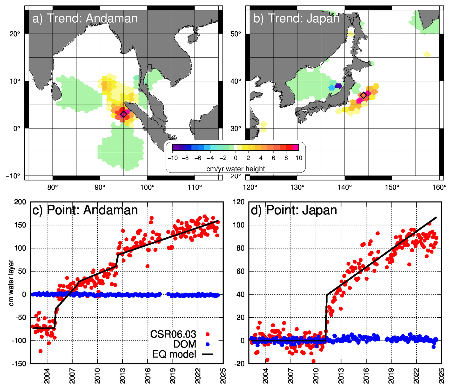
Figure 5 2002–2025 Trend of CSR RL06.3 standard mascon series near (a) Andaman Bay and (b) Japan), plus timeseries (c, d) of a single mascon near each epicenter (locations shown as diamonds in a and b) for both CSR RL06.3 (red) and the DO mascons (blue). Timeseries of the earthquake model at the observed points is shown as the black line. (Global ocean means have been removed from RL06.3 each month, to approximate the removal of the GRD signal.)

2.3 Earthquake model

Any oceanographer or sea level scientist who has tried to use GRACE/FO data in the northwestern Pacific or northern Indian Oceans has observed the enormous solid earth gravity signal caused by the two largest oceanic earthquakes which have occurred since GRACE's launch. The Andaman-Sumatra magnitude 9.2 earthquake occurred on 26 December 2004 and is easily visible (Fig. 5a) in any regional or global GRACE analysis (Han et al., 2006; Chen et al., 2007; Han et al., 2008; De Linage et al., 2009), as is the magnitude 9.0 Tōhoku, Japan earthquake (Fig. 5b) of 11 March 2011 (Cambiotti and Sabadini, 2012; Wang et al., 2012; Fuchs et al., 2013; Dai et al., 2014). Both megathrust earthquakes caused a shift in the solid earth gravity signal around the epicenter at the time of the earthquake (the co-seismic effect) and a long-term, near-linear drift after the earthquake (the post-seismic effect) which continues through this day (Fig. 5b). The Andaman situation is complicated by subsequent quakes in the same area. Various mascon solutions attempt to accommodate this highly localized gravity signal, but as Bonin et al. (2026) demonstrate, the pattern and magnitudes of the resulting mascon signal vary among GRACE/FO processing centers and are dependent on specific regularization and background model choices.

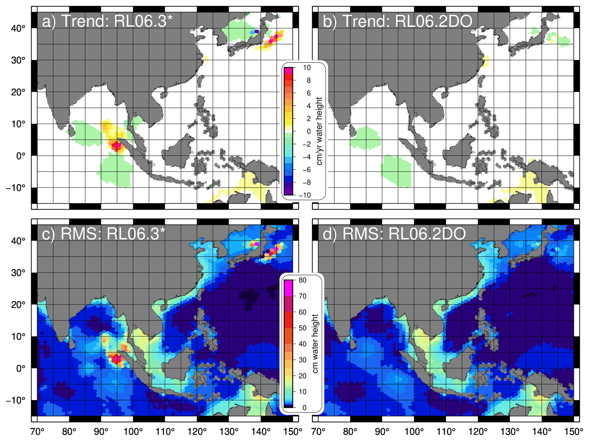
Figure 6 Trend and RMS of (a, c) the CSR RL06.3 mascons after the barystatic-GRD and GAD_avg have been removed, and (b, d) the DO mascons, from 2002–2023.

In the Andaman-Sumatra area, the CSR RL06.3 mascons observe a co-seismic jump of approximately 50 cm for the largest earthquake in 2004, with smaller jumps for subsequent earthquakes, along with up to 6 cm yr⁻¹ post-seismic trends (after the last quake). The Tōhoku earthquake has a similar effect: about a 40 cm co-seismic bias near the epicenter, and a ∼ 5 cm yr⁻¹ trend in the decade afterwards. These gravity changes are an order of magnitude larger than observed sea level or ocean mass change (which is generally less than 0.3 cm yr⁻¹ once barystatic-GRD is removed) and must be removed before the DO mascons can be considered useful for ocean dynamic studies in the region. We have estimated the non-oceanographic mass signals induced by the two earthquakes mentioned above, plus two subsequent quakes in the Andaman Bay area (in September 2007 and April 2012) using a localized principal component analysis (PCA) to isolate the two largest PCA modes. This model explains ∼ 98 % of the local signal variance (Bonin et al., 2026; Pie and Bonin, 2025). The details of the methodology are beyond the scope of this paper but are described in Bonin et al. (2026). We demonstrate here that the recovered model matches the extreme mass signals quite well (Fig. 5c and d), and that after removing the model, the variance of the GRACE RL06.2DO mascons (and trends) is reduced to levels expected from oceanographic processes based on ocean mascons nearby (Fig. 6).

The earthquake model was estimated using the GRACE RL06.2 mascon data between April 2002 and February 2023. We extended the model's final linear fit from March 2023 to May 2024, which corresponds to the end of the RL06.2 series. We then included this earthquake model in the estimation background model as part of the Level-2 mascon processing stream used to estimate the new CSR RL06.2DO mascons. We did not simply subtract the model from the original mascons as a post-processing step, and do not recommend that the model we include in the dataset be used for this purpose on any other mascon data set. As Bonin et al. (2026) demonstrated, by applying this earthquake model as a background model for the CSR mascon estimation processing, we are able to drastically tighten the constraints there. If one did not do this and simply removed the model from the GRACE RL06.2 mascons, there would be increased noise in the area of the earthquake because the RL06.2 constraints are relaxed to allow the earthquake signal into the proper mascons. For example, the residual standard deviation around the earthquake model at the epicenter of the Andaman-Sumatra earthquakes using the looser RL06.2 constraint is 8.5 cm, which is 4 times higher than for an ocean mascon far away from the epicenter (< 2 cm) (Fig. 6c and d). By applying the earthquake model as part of the processing stream, we improve the signal-to-noise ratio near the earthquake regions, resulting in reduced residual DO mascon noise levels over other mascon solutions, in addition to the obvious benefit of separating the solid earth signal from the desired ocean signal.

We provide the earthquake model used (Pie and Bonin, 2025) for users interested in the earthquake signal that was removed, and for those interested in restoring the earthquake model to obtain mascons less noisy in this region than the standard CSR RL06.2 mascons. However, our earthquake model grid should not be removed from mascons produced by other processing centers (e.g., Jet Propulsion Laboratory or Goddard Space Flight Center), or from gridded spherical harmonics, because these have different earthquake patterns that are dependent on their processing, background models, and regularizations used (Bonin et al., 2026).

2.4 GRD and barystatic ocean mass signals

There is a substantial time-variable exchange of mass between the oceans and the land/ice, on both a long-term and an annual-scale time frame (Fig. 7a), with the global average change in the ocean termed “barystatic” (Gregory et al., 2019). The associated gravitational, rotational, and deformational (GRD) effects caused by this mass motion creates large-scale, non-uniform patterns in ocean mass represented by the mascons (Fig. 7b and c) (e.g., Farrell and Clark, 1976). The combined barystatic-GRD signal will not cause significant dynamic ocean signals, since redistribution of mass within the ocean occurs rapidly, leading ocean pressure to reach equilibrium (meaning negligible horizontal pressure gradients) far faster than the seasonal or longer timescale characteristic of barystatic-GRD effects (Ponte, 2006). The signal is largest near glaciated regions losing significant amounts of mass into the ocean (high negative trends in Fig. 7b around Greenland, Alaska, Patagonia, and West Antarctica), with a balancing far-field rise in ocean interiors. While trends are strongest near ice sheets, annual amplitudes are highest near large hydrological basins with strong seasonality that peaks at the same time as global ocean mass, such as the Bay of Bengal (Fig. 7c). Annual GRD signals near land may alternatively be suppressed, if the water storage in the basin peaks during the global ocean mass minimum (e.g., the Amazon) (Fig. 7c). A related signal arises from global ocean-area atmospheric pressure variations, seen as the average of the GAD product over the oceans (Fig. 7a, blue line). This signal is defined to be uniform over the ocean.

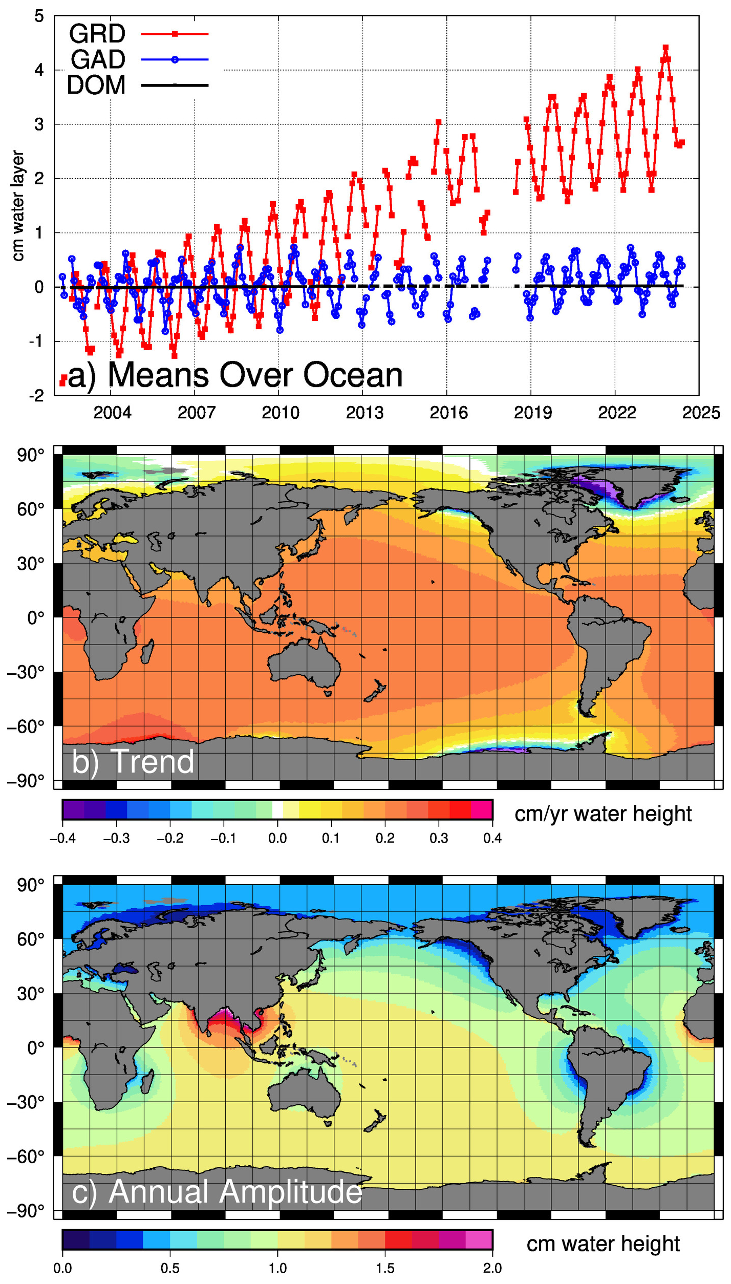
Figure 7 Mass exchange between the ocean and the rest of the globe, via: (a) mean signals over the global oceans, for the barystatic-GRD, the GAD, and the dynamic ocean mascons; and (b) trend and (c) annual amplitude distribution of the barystatic-GRD estimate.

The standard mascons represent both internal ocean pressure variations (which drive geostrophic balance), GRD mass signals, and the atmospheric pressure variation estimated by GAD. Because internal pressure variations should average out to zero, global averages of the standard mascons reflect a combination of GRD and this atmospheric pressure signal (e.g., Chambers and Schröter, 2011). We intend the DO mascons to reflect only the portions of the ocean pressure signal that impacts geostrophic balance, and thus remove both the barystatic-GRD signal and the mean atmospheric pressure signal over the global oceans, resulting in monthly global ocean mean values of zero at all times in the DO mascons (Fig. 7a, black line).

Figure 7 shows only the estimated trend and annual amplitude of GRD, but we calculate the full barystatic-GRD signal over the same quasi-monthly period the mascons are computed over, based on the methods described in Tamisiea et al. (2010). This captures the full month-to-month variations and interannual changes as well. For this calculation, we use the DO mascons over land as an estimate of the hydrological+ice changes, which complements and drives the barystatic-GRD changes. As in many GRD calculations, the contribution of dynamic ocean and atmospheric mass changes to the GRD estimate are not considered for two reasons. First, relative to the barystatic-GRD signal caused by land/ice changes, the impact of the ocean and atmosphere mass change on the barystatic-GRD is small. The most significant impact is on the annual amplitudes, with differences in the barystatic-GRD estimates generally less than 0.5 cm except around the coasts of Eurasia and Antarctica.  Second, because results incorporating the GRACE AOD1B RL06 into the barystatic-GRD estimate were ambiguous as to whether improvement was achieved. We choose to omit that relatively small contribution here. In addition, because GRACE cannot independently estimate the spherical harmonic degree 1 variability of mass change, we simultaneously estimate it (similar to Sun et al., 2016a, b) to be consistent with the mascons and barystatic-GRD estimate. It must be noted that rotational signals have been removed from the GRACE data in the standard background models, and thus rotational components are not included in the barystatic-GRD estimate. The GRD series which results is similar to the recent JPL barystatic-GRD series (Landerer and Wiese, 2025), but computed using the land input from the DO mascons rather than the JPL mascons. Average differences between these barystatic-GRD series (Fig. B1) are only 0.01 cm yr⁻¹ in trend and 0.06 cm in annual amplitude. The recent GravIS barystatic-GRD series (Fig. B2) is substantially different from either the DO or JPL barystatic-GRD series, probably because it is based on spherical harmonic input rather than mascon input (see Appendix B).

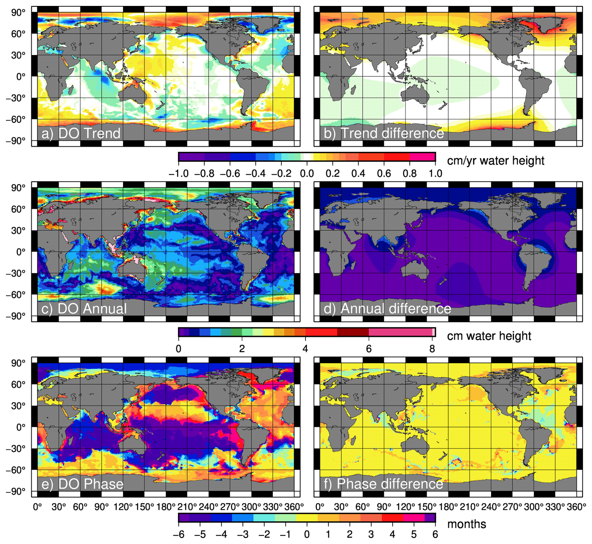
Figure 8 The 2002–2024 trends (a), annual amplitudes (c), and annual phases (e) of the DO mascons, compared to the changes away from a comparison case where a uniform global ocean average is removed rather than the GRD estimate (b, d, and f). Phases in (e) are defined such that 0 refers to an annual maximum in January, and ± 6 refers to a maximum in July. Phase differences in (f) are the number of months that the comparison series' phase is shifted away from the DOM phase.

The monthly barystatic-GRD estimates are removed, along with the monthly GAD average over the ocean, to create the DO mascons. In doing this, we create a series of ocean mascons that have zero ocean-average mass change (Fig. 7a, black line), so that they will only show internal mass redistribution from ocean dynamics. Previous studies have attempted to estimate such grids for ocean applications (Song and Zlotnicki, 2008; Chambers and Willis, 2009; Landerer et al., 2015) by removing a uniform ocean mass signal (i.e., the time series shown in Fig. 7a applied uniformly for each grid cell). In Fig. 8 (right), we depict the errors caused by removing such a uniform ocean mass signal to approximate land/ice drainage, rather than removing the full barystatic-GRD estimate of ocean mass redistribution. These errors are a substantial fraction of the full DO mascon signal (Fig. 8, left) for the trend and annual amplitude, and (unsurprisingly) have the same spatial patterns as the GRD trend and annual amplitude (Fig. 7). Maximum trend differences are greater than 1 cm yr⁻¹ just off the coast of Antarctica and Greenland (Fig. 8b), compared to local DO mascon trends less than half that size. Changes in the annual signal amplitude exceed 1 cm near the Amazon, the Ganges, and the Alaskan glaciers (Fig. 8d), similar to what Ponte et al. (2024) noted when using the recent JPL GRD estimate (Landerer and Wiese, 2025). While, in most places, changes in the phase of the annual signal (Fig. 8f) are less than a month, using a simplified uniform distribution instead of a true barystatic-GRD approach shifts the timing of the annual by a month or more over substantial fractions of the ocean. These differences are seen as non-oceanographic artifacts left in any GRACE/FO series that does not remove a barystatic-GRD estimate. By estimating and removing GRD from the DO mascons, we avoid such artifacts (Fig. 8a, c, and e).

The barystatic-GRD estimates affiliated with the dynamic ocean mascons are provided separately (Pie et al., 2025), in case users want to reapply them and/or remove their own GRD estimate.

3 Dynamic ocean mascon statistics

We produced the dynamic ocean mascons using GRACE/FO data from April 2002 until May 2024, matching the full run of the RL06.2 data. The main product is provided with the earthquake model, barystatic-GRD effects, and the average of GAD over the ocean removed, such that the product is ready for oceanographic use. We have already demonstrated (Fig. 7a, black line) that total ocean mass remains constant in this series. We now show the linear trends (Fig. 9), annual amplitude (Fig. 11), and RMS of the residual with the bias, trend, annual, and semiannual removed (Fig. 13) for the DO mascons, the most modern standard CSR mascon series (RL06.3) after the ocean mean has been removed each month, and ocean bottom pressure from the ECCOv4r4 ocean state estimate (ECCO Consortium et al., 2021a, b; Forget et al., 2015). Maps of the differences between the DO mascons and ECCOv4r4, and between the RL06.3 comparison and ECCOv4r4, are shown in Appendix C, with only the averaged statistics given here.

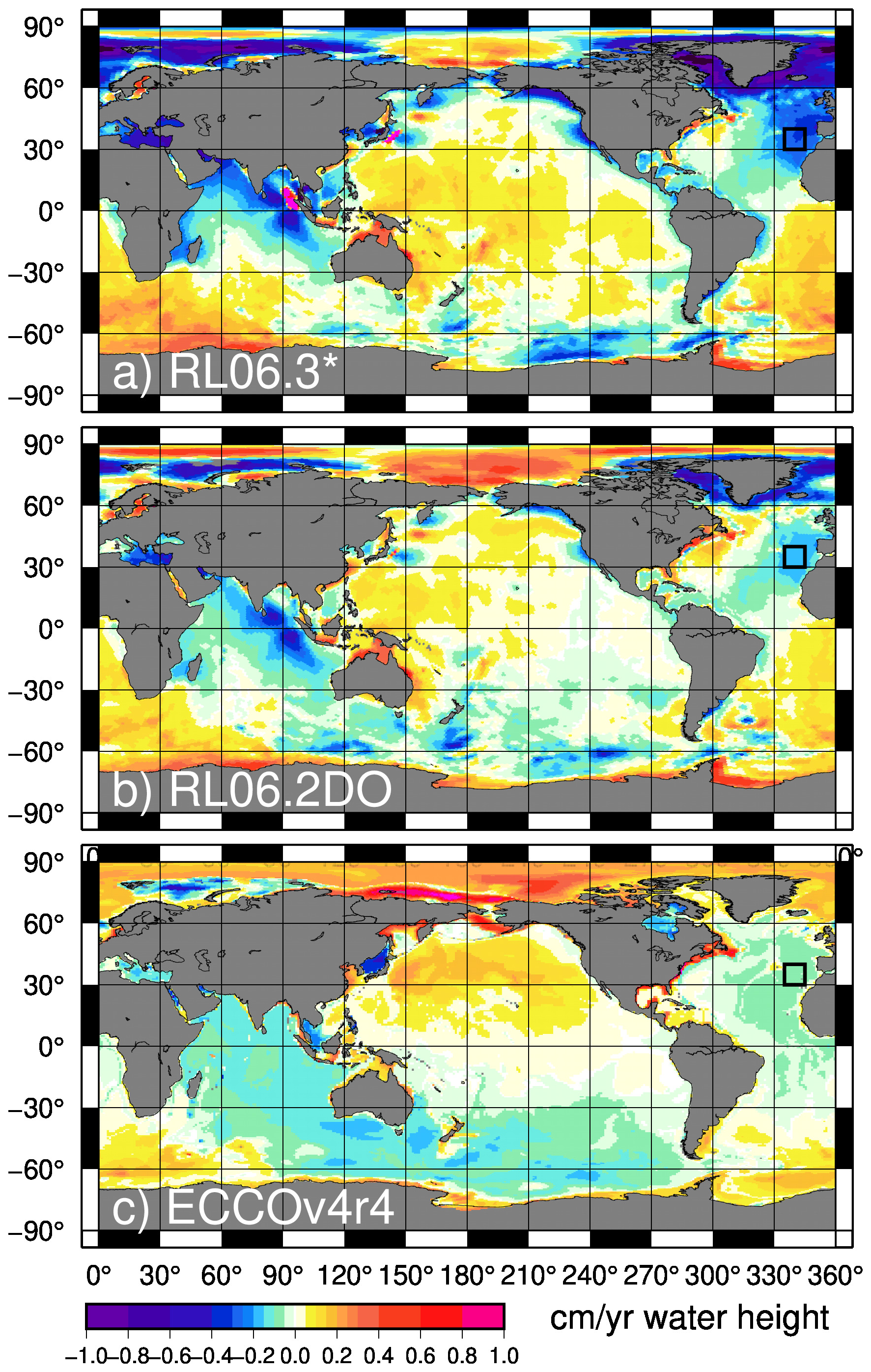
Figure 9 2002–2017 trends from (a) CSR RL06.3 mascons after a uniform global ocean average is removed each month, (b) the DO mascons, and (c) the ECCOv4r4 model. Black box denotes the region averaged over to calculate the timeseries in Fig. 10.

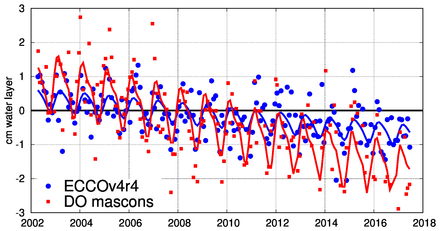
Figure 10 Average mass change (in terms of water height) in the region of the northeastern Atlantic drawn in Fig. 9.

We want to note that ECCOv4r4 incorporates GRACE data as constraints to their bottom pressure estimates during their weighted-least-squares optimization process, in which they adjust boundary conditions, initial conditions, and model parameters to best minimize the model-minus-observation misfit. Due to this, there is some concern that the ocean bottom pressure estimates of ECCOv4r4 could be pulled towards GRACE by the optimization process itself, even if GRACE is more incorrect than the unconstrained model. Two facts convince us that a similarity with ECCOv4r4 is not merely an echoed recognition of GRACE's assimilation into the state estimate, however. First, the assimilation uses the 2002–2016 GRACE JPL RL05 mascon data, which is significantly different in both mascon averaging size and detailed ocean statistics from our 2002–2024 CSR RL06-based DO mascons. Second, ECCOv4r4 also simultaneously assimilates millions of non-GRACE observations (ECCO Consortium, 2021b), and the assimilation method finds the state variables that statistically optimize the residuals between all assimilated observations, not just GRACE. Thus, if ECCOv4r4 agrees with GRACE mascons, it means that the model physics and other (more numerous) observations were statistically consistent with the GRACE data, not that ECCOv4r4 is automatically adjusted toward GRACE. For example, the strong difference between ECCOv4r4 and our GRACE/FO DO maps in the eastern Atlantic (Figs. 9 and 10; discussed below) is an indication that the assimilation rejected the GRACE observations there as being inconsistent with the model physics and other observations and so did not significantly adjust the estimated result toward GRACE.

Removing the monthly ocean mean from RL06.3 mimics the simple GRD-like removal that many ocean scientists have historically used (Song and Zlotnicki, 2008; Chambers and Willis, 2009; Landerer et al., 2015), such that the impact of RL06.2DO's more accurate barystatic-GRD estimation can be fairly evaluated. Please note that the ECCOv4r4 series (henceforth “ECCO”) includes a non-zero, time-varying global mean term to approximate water mass exchanges between land and ocean within the model. We subtract this monthly, uniform layer to make it more consistent with the DO mascons. Comparisons between ECCO and the DO mascons are not appropriate without such a correction applied, in the same way that a comparison between RL06.3 and the DO mascons would not be appropriate without first removing the RL06.3 ocean mean. Calculations are made from 2002–2017, the timespan when ECCO and GRACE/FO overlap.

3.1 Trend Analysis

There are substantial changes between the DO mascons and ocean-mean-removed RL06.3, particularly in terms of the Arctic-area linear trend (Fig. 9), which is much closer to zero in the DO mascons. Trend reductions across the Pacific Ocean are also visible. Most of this change is due to the removal of the barystatic-GRD signal, as opposed to the simpler technique of merely removing an ocean-wide mean for each month. Such changes are anticipated – for example, Ponte et al. (2024) demonstrated that incorporating a barystatic-GRD signal (their “GAL” or “Gravitational Attraction and Loading”) improved the fit between the JPL GRACE mascons and ECCO over 56 % of the ocean's area, and made particularly large improvements in coastal regions near large land/ice mass sources like Greenland and coastal Alaska, similar to what we see here. Trend differences also occur near Franz Josef Land in the Arctic (see also Fig. 3), where the land/ocean mask and constraints were altered to more appropriately localize the land ice signal and prevent leakage into nearby ocean mascons. Close around the earthquake regions, there are large local improvements caused by the removal of the model and the constraint tightening.

Table 1 Comparison of standard deviations, linear trends, annual amplitudes, and residual standard deviation (after the removal of trends, annuals, and semiannuals) of the ECCOv4r4, DO mascon, and CSR RL06.3 with mean ocean mass uniformly removed, as well as the same statistics for the differences between each mascon series and ECCOv4r4. The “open ocean” is defined as CSR ocean mascons more than 300 km, exclusive of the Arctic and earthquake regions. The “open equatorial” is defined as the subset of the “open ocean” within 30° of the equator. The “earthquakes” region is defined as the broader regions near Japan and Andaman Bay modelled in Bonin et al. (2026). Bold values indicate the GRACE/FO series with the smallest difference from ECCO.

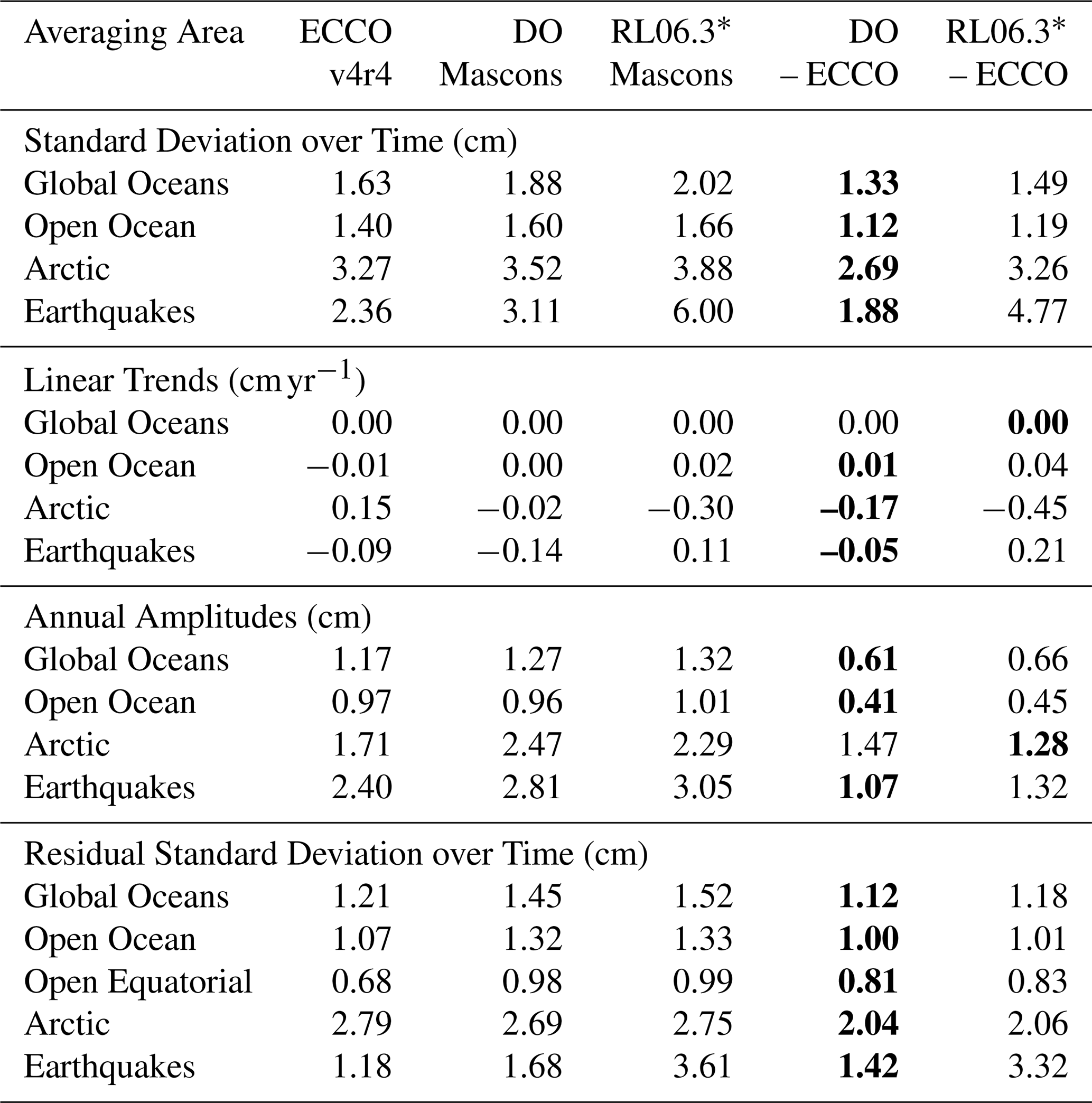
By removing barystatic-GRD, the earthquake signal, and the effect of mean atmospheric pressure, we have created a series of mascons which reflects expected ocean dynamical variations better than the standard RL06.3 series can. For example, the DO mascons show mass losses in the Indian Ocean and Southern Ocean and rises in the South Atlantic, which are more consistent with the ECCO state estimate. Overall, we find that the DO mascon trends are generally both nearer to zero and more similar to ECCO than the RL06.3 trends are (Fig. C1, Table 1), with an improvement of 0.022 cm yr⁻¹ in the non-arctic open ocean (defined as ocean grids more than 300 km from land, exclusive of the Arctic Ocean and the regions involved in the earthquake modelling). In the Arctic Ocean, the trend reduction from RL06.3 is more pronounced: a difference of 0.28 cm yr⁻¹. Near the earthquakes, the change is 0.26 cm yr⁻¹. In all cases, these differences are larger than the trends in each area seen in ECCO alone, and in each area, the change drives the trends both closer to ECCO and closer to zero. We therefore assume that the trends of the DO mascons represent improvements over the RL06.3 trends with a uniform ocean mean removed.

While the model used in the DO processing has removed most of the variance caused by the earthquakes near the epicenters, some trends remain in the northern Indian Ocean and the northwestern Pacific Ocean that are not entirely consistent with the larger-scale ocean trends in the area. These questionably large trends are most obvious 5–15° away from each earthquake epicenter, well outside the region of greatest impact, and explain a significant fraction of the DOM signal in these regions (over 70 % of the signal west of the Andaman quakes, and 20 %–40 % near Japan). Long-term signals, especially linear trends, are expected to be the least accurate part of the earthquake model (Bonin et al., 2026), because the EOF method used to construct the model cannot easily distinguish between a trend caused by ocean dynamic changes, a trend caused by solid-earth post-seismic motion of a prior earthquake, and a “trend” which is really a sudden co-seismic jump during an earthquake. The majority of this confusion was treated during a pre-processing step to the earthquake modelling (Bonin et al., 2026), but we expect that some misappropriated long-term solid-earth signal remains in the DOM due to an imperfect earthquake fit. An unknown but probably large percentage of the near-earthquake DOM trends (and potentially other long-period signals) are likely to be residual long-wavelength solid earth signals not removed by the earthquake model. We recommend oceanographers working in these regions consider removing trends from the DO mascons and only use the residuals in their analysis. In the northern Indian ocean, west of the Andaman-Sumatra sequence of earthquakes, a smaller change in trend seems to occur after the final April 2012 quake, which some users may find beneficial to fit and remove locally as well. (This 2012 trend change will not impact the Japanese quake area, nor will the earthquake model trend uncertainty impact any area away from the earthquakes.)

The DO mascons also have significant non-zero negative trends east and west of Greenland (Fig. 9), especially in Baffin Bay, which are not present in ECCO. While the removal of GRD reduces these trends from the original mascons (Fig. 9b vs Fig. 9a), the remaining trends are still substantial and generally in the same direction as ice mass loss from Greenland. Because ECCO does not suggest significant bottom pressure trends in these regions, and since the regions are bordered by large ice mass losses on both sides, we suspect these signals are due to residual leakage and suggest caution when using the DO mascons near Greenland.

The final area with a significant trend difference from ECCO is in the northeastern Atlantic, where the DO mascons suggest a large (−1.8 mm yr⁻¹) drop in mass/bottom pressure, while ECCO suggests a much smaller (−0.7 mm yr⁻¹) change (Fig. 10). This signal is not unique to the DO mascons. It appears as an even larger trend in the standard mascons (Fig. 9a), as well as mascons and gridded spherical harmonics from other processing centers. This indicates it is probably a real gravity signal that the GRACE/FO observations must accommodate, not some sort of error due to (for example) a specific version of mascon regularization. However, it is difficult to theorize an ocean dynamic signal which could cause such a large linear trend over the course of the entire GRACE/FO mission. While the lower limb of the Atlantic Meridional Overturning Circulation (AMOC) does cause bottom pressure variations (Bingham and Hughes, 2006; Elipot et al., 2014; Landerer et al., 2015; Frajka-Williams et al., 2018), ocean mass transport on the western side of the Atlantic is an order of magnitude larger than on the eastern side. Moreover, a large drop in pressure on the eastern side would also suggest a large increase in the southward flow of the AMOC lower limb, which has not been observed in any of the instrumented arrays measuring the upper limb transport across the Atlantic (Smeed et al., 2018; Johns et al., 2023; Volkov et al., 2024). These studies show either a small decrease in upper limb transport across 26.5° N latitude or no decrease, which is inconsistent with the bottom pressure signature in the GRACE/FO mascons north of the latitude. A difference in the sign of change in the transport between the lower and upper limbs of AMOC across 26.5° N is impossible from mass conservation, as it would cause a drop in sea level over the entire North Atlantic of several meters, which has never been observed.

Thus, we conclude that the bottom pressure trend observed in all GRACE (and presumably GRACE-FO) data in the northeast Atlantic cannot be oceanographic in nature. It is beyond the scope of this study to determine what could be responsible for the signal, but we suspect it is a solid earth gravity signal that deserves further investigation, potentially a signal inside the mantle (Gouranton et al., 2025) or along the core-mantle boundary (Mandea et al. 2015). We would recommend any studies of AMOC transport based on east-west gradients of bottom pressure across the Atlantic using the GRACE/FO data (e.g., Landerer et al., 2015) to continue to remove local trends and only consider non-linear transport variations.

3.2 Annual analysis

The DO mascon annual amplitudes (Fig. 11) are also more similar to ECCO, and in expected areas are consistent with seasonal ocean dynamics (e.g., Johnson and Chambers, 2013), such as seasonal changes in the Pacific subtropical gyres, the Indian Ocean circulation, and closed potential vorticity ($f/H$) contours in the Southern Ocean. The annual dominant fluctuation in the North Pacific, related to seasonal changes in wind stress curl (e.g., Chambers, 2011), is clearer in the DO mascons. Decreases in the annual amplitude can be seen around northern coastal South America, where the DO mascon signal is more like ECCO than the RL06.3 signal is (Fig. C1e vs. Fig. C1f). These are likely improvements due to the better barystatic-GRD treatment, as were also seen by Ponte et al. (2024).

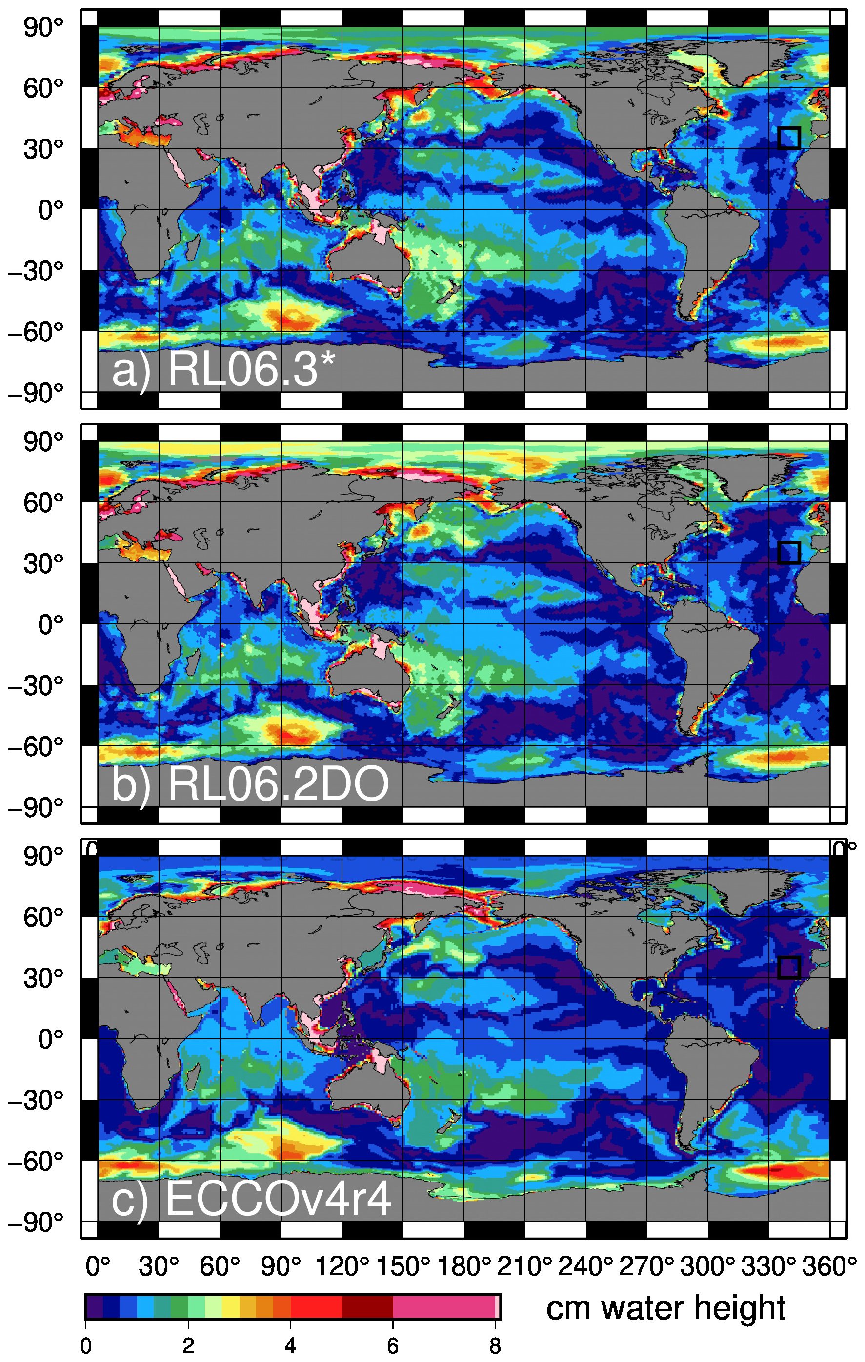
Figure 11 2002–2017 annual amplitudes from (a) CSR RL06.3 mascons after a uniform global ocean average is removed each month, (b) the DO mascons, and (c) the ECCOv4r4 model.

Across the global oceans, the annual amplitude of the differences between the DO mascons and ECCOv4r4 is slightly smaller (0.61 cm) than the similar difference between the RL06.3 mascons and ECCO (0.66 cm). A similar 0.04 cm improvement exists in the open ocean, and a larger 0.25 cm improvement near the earthquakes (Table 1). The 2002–2017 phase of the annual (not shown) closely matches that of the 2002–2024 series (Fig. 8e), which are also similar to phase maps found in the modern JPL and GSFC GRACE/FO mascons (Ponte et al., 2024), with phases consistent across latitudes through the Indian and Pacific Oceans, and the Atlantic and Arctic differing from both. In most places, the annual phase of the DO mascons is within half-month (± 15°) of the ECCO state estimate (Fig. 1g), though there are stripes of considerable phase variability throughout the ocean, where a simple annual amplitude difference may not fully explain the errors. However, phase differences of more than half a month typically occur in regions where the annual amplitude is small. The average absolute value non-Arctic, open-ocean phase difference from ECCO, in places with over 1 cm annual amplitude, is 0.36 months for the DO mascons versus 0.43 months for the RL06.3 mascons (Fig. 1h). This suggests that the DO mascons improve the annual phase resolution in places where the annual signal is strongest.

In the Arctic, however, the amplitude of the residual annual signal is 0.19 cm smaller when differencing ECCO from RL06.3, than from the DO mascons (Fig. C1, Table 1), and the DO mascon phase there is slightly more offset from ECCO's as well (Fig. C1g and h). We believe that this shows that the DO mascons capture an Arctic signal that is not represented in the ECCO model, rather than evidence of enhanced errors in the DO mascons over the standard CSR mascons. Previously, the ocean near the North Pole has been shown to have large seasonal mass variations and compare well between pressure gauges and early GRACE data (Peralta-Ferriz and Morison, 2010; Peralta-Ferriz et al., 2016), which are not well-estimated by ECCO. The ECCO state estimate peaks in June and decays rapidly thereafter, while the central-Arctic DO monthly climatological signal ramps up until June but remains high from then through October (Fig. 12). Considering the limited observations that ECCO runs can assimilate in the Arctic (compared to the rest of the ocean) and the fact that previous studies have shown strong agreement between bottom pressure recorders and GRACE, we assume this reflects a true ocean signal observed in the DO mascons that is not captured by ECCO, and captured less well by the standard RL06.3 CSR mascons.

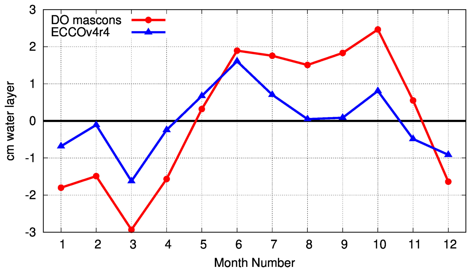
Figure 12 Differences in monthly climatology of average within 5° longitude of the north pole.

3.3 Non-seasonal variability and uncertainty analysis

Non-seasonal variability in the DO mascons has similar magnitude and locations as that seen in ECCO (Fig. 13), with the largest variability at high latitudes and lower values at the equator. The equatorial variance away from the coastlines (“open-equatorial” in the bottom of Table 1) is often used as a standard measure of the noise floor in the DO mascons. The level of high-frequency (non-annual) variability there should be quite small, with standard deviation well below 1 cm. Average ECCO open-equatorial RMS residuals are 0.68 cm (Fig. 13b, Table 1), confirming the approximate RMS of the expected signal. The DO mascons have a value 0.30 cm higher than this (average values 0.98 cm). Based on the residual of the DO mascons and ECCO (Fig. 3c, Table 1), ∼ 0.8 cm RMS is a reasonable approximation of the month-to-month uncertainty in the DO mascons. We do note, however, that this estimate could underestimate the errors, if the assimilation of GRACE/FO causes larger artificial similarities than we assume.

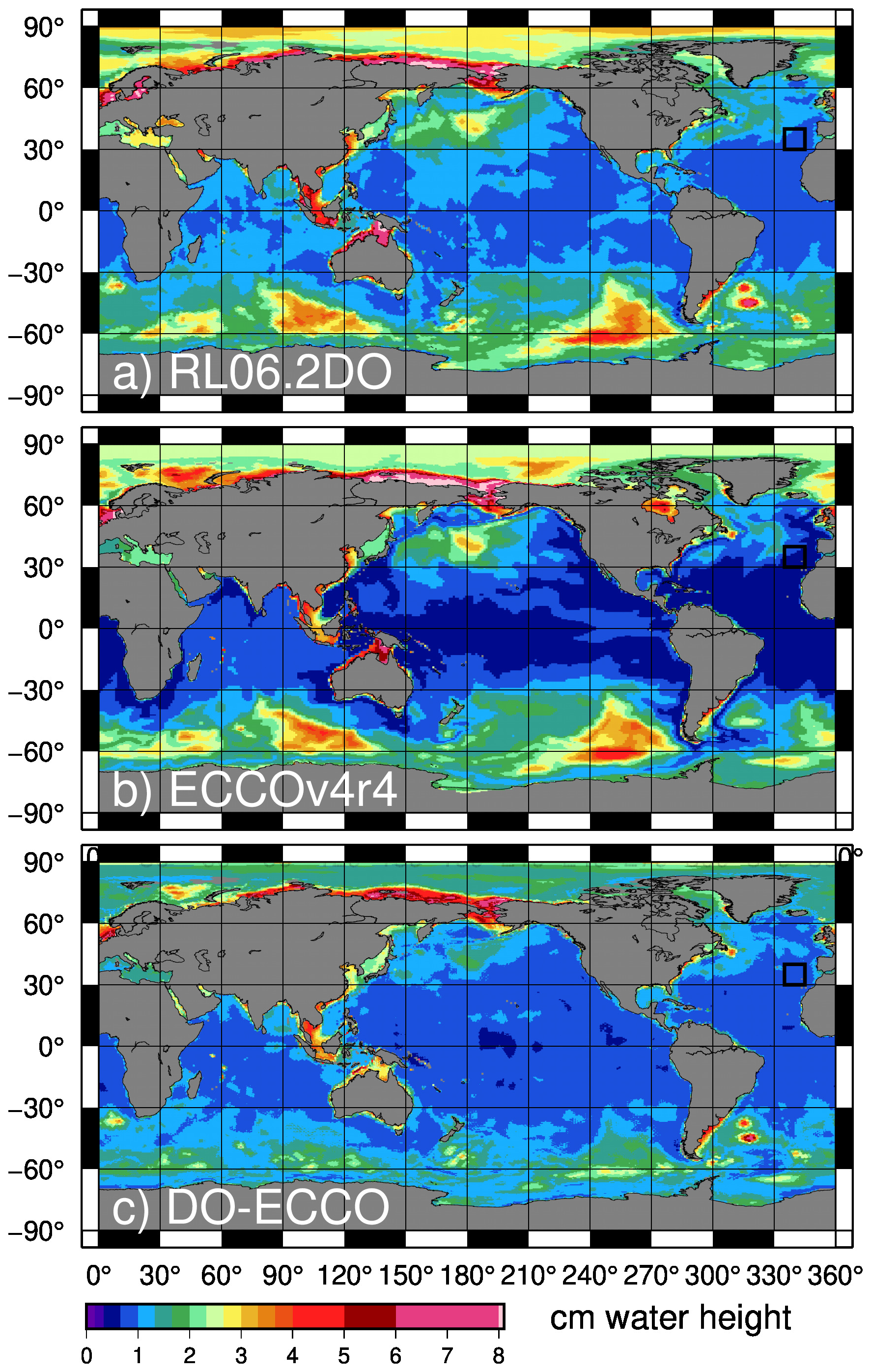
Figure 13 2002–2017 residual RMS from (a) the DO mascons, (b) the ECCOv4r4 model, and (c) differences between the two. Trend, annual, and semiannual effects have been removed.

In reality, the uncertainty as measured by comparison with ECCO varies with region, with differences larger at higher latitudes due to greater ocean model uncertainty, near coastlines (especially Arctic/Antarctic ones) due to GRACE/FO ice/land leakage, and near the major earthquakes due to earthquake model uncertainty. Based on the differences with ECCO (Table 1), we estimate DO mascon uncertainties near the earthquakes to be 1.42 cm (much smaller than the RL06.3 uncertainties of 3.32 cm). The Arctic area uncertainties for the DO mascons are found to be 2.04 cm (compared to a similar 2.06 for RL06.3). These differences with ECCO represent an expected upper bound on the DO mascon uncertainties, because they include any errors in the state estimate as well as the GRACE/FO errors. For example, we suspect the Arctic uncertainties to be overstated, because we anticipate that a large part of the differences in the Arctic are due to missing signal in ECCO. Another signal seen in the DO mascons and not ECCO is the high variability in the Argentine basin east of Brazil (Fig. 13), which has a known, sub-annual barotropic variation (Fu, 2007; Hughes et al., 2007; Yu et al., 2018). It is greatly damped in ECCO (and the ocean dealiasing product used for GRACE/FO processing), but is recovered better by GRACE/FO mascons, both the original and the DO versions. In locations such as this, the difference between ECCO and the mascons will overstate the DO uncertainties.

4 Data availability

The standard CSR RL0602 mascon series that this work was based upon has since been superseded by the very similar CSR RL0603 data. Those mascon series are freely available at https://www2.csr.utexas.edu/grace/RL06_mascons.html (last access: 3 November 2025). A link to information concerning the older processing scheme still exists, though its data series are no longer accessible there: https://www2.csr.utexas.edu/grace/RL0602_mascons.html (last access: 20 May 2026).

The resulting dynamic ocean mascons are available at the Texas Data Depository (Pie et al., 2025) at https://doi.org/10.18738/T8/3VUPEW. The barystatic-GRD estimate (dataset: “CSR_GRACE_GRACE-FO_RL06.2DO_Mascons_GRD-component.nc”) and earthquake model (dataset: “CSR_GRACE_GRACE-FO_RL06.2DO_Mascons_EQ-component.nc”) are also available there as separate files.

5 Conclusions

The dynamic ocean mascons are available at the Texas Data Depository (Pie et al., 2025). The barystatic-GRD estimate (dataset: CSR_GRACE_GRACE-FO_RL06.2DO_Mascons_GRD-component.nc) and earthquake model (dataset: CSR_GRACE_GRACE-FO_RL06.2DO_Mascons_EQ-component.nc) are also available, if users care to investigate those or restore them and remove their own estimates. The new mascons extend from the start of GRACE (April 2002) through the end of the CSR RL06.2 series (May 2024), making a total of 22 years of data. Gaps exist for those months where data does not exist in other GRACE/FO series, including the year-long gap between June 2017 and June 2018, between the two missions.

The dynamic ocean mascons (with the removed components added back) are very similar to the CSR RL06.2 (and RL06.3) mascons they were based on, except for changes in the earthquake and Franz Josef Land areas, near polar coastlines, and in the geocenter term (a smaller but global effect). The primary benefit of the series is ease of use: oceanographers do not need to be experts in GRACE/FO processing to use this data for research. Like other mascon series, the data is in a simple gridded format that does not require spherical harmonic knowledge to read. The gravity signals which are caused by ocean dynamics have been partitioned from the non-ocean-caused gravity signals, properly accounting for mass variations caused by mass exchange with land, barystatic-GRD, the solid earth motion due to four large oceanic earthquakes, and the effect of global atmospheric pressure. Because most non-oceanographic signals have already been removed, this product is expected to be an easy starting point for oceanographic use.

The dynamic ocean mascons are designed to be comparable to ocean models (once conservation of mass is taken into account within the model). We remind users that this is a measure of dynamic ocean mass change, not a measure of bottom pressure. The dynamic ocean mascons should not be directly compared to ocean bottom pressure recorders or models of ocean bottom pressure (unless the impact of water mass addition to the ocean via barystatic-GRD has been considered). They also should not be directly compared to any ocean model with non-zero mean mass change across the ocean (including the standard ECCOv4r4 release, unless you also remove the monthly ocean means). The dynamic ocean mascons, however, are useful for comparisons to mass-conserving models, for assimilation into ocean models, and for comparisons with or estimates of dynamic ocean signals.

Appendix A: Constraint sigmas for related CSR mascon series

The “sigmas” of the CSR mascon constraints have been changed substantially over the Arctic Ocean, during the various RL06 releases. For clarification, we show the changes between RL06.1, RL06.3 (identical to RL06.2), and the new RL06.2DO, in terms of climatologies. Note that, unlike the other two cases, the RL06.2DO mascons do not use the actual climatology shown, but instead have different values for each individual month (e.g., Fig. 2 in the main text).

The technique used to estimate the RL06.2DO sigmas can potentially lead to undesirably reduced sigmas in cases when a month's GAD signal is atypically high compared to the climatology. The monthly value will then be ignored, in favor of the lower climatology value. In practice, however, the GAD climatology is typically at or above the 5 cm limit along the coastlines where sigmas are above the 3 cm minimum – see Fig. 2 – such that this is rarely a problem.

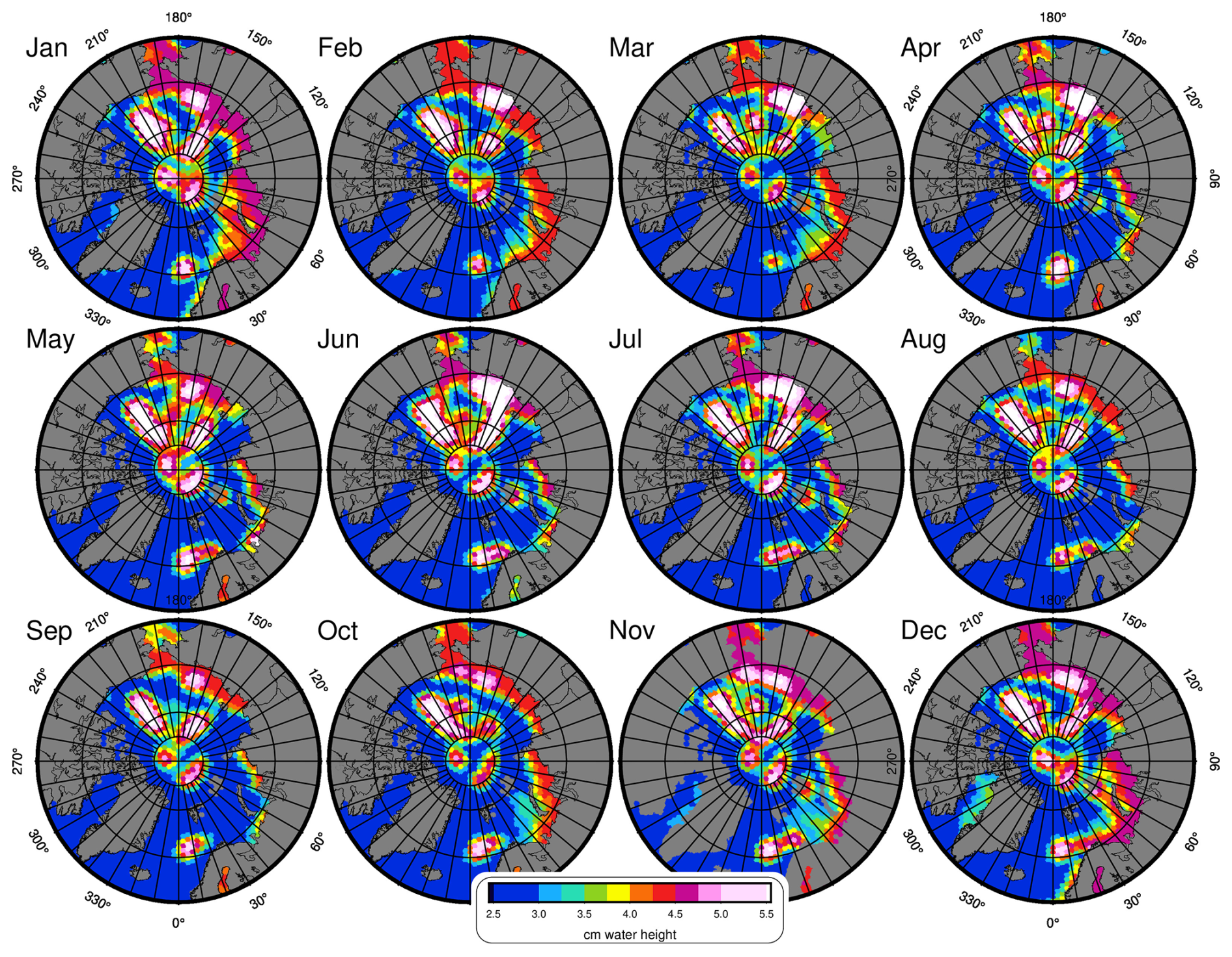
Figure A1 Arctic ocean climatology of CSR RL06.1 constraint sigmas. This is based on RL05 CSR mascons and contains “stripe-like” values in the arctic which do not realistically represent ocean variance.

Figure A2 Arctic ocean climatology of CSR RL06.3 constraint sigmas. This is based on the GAD climatology, with min/max boundaries of 3–5 cm.

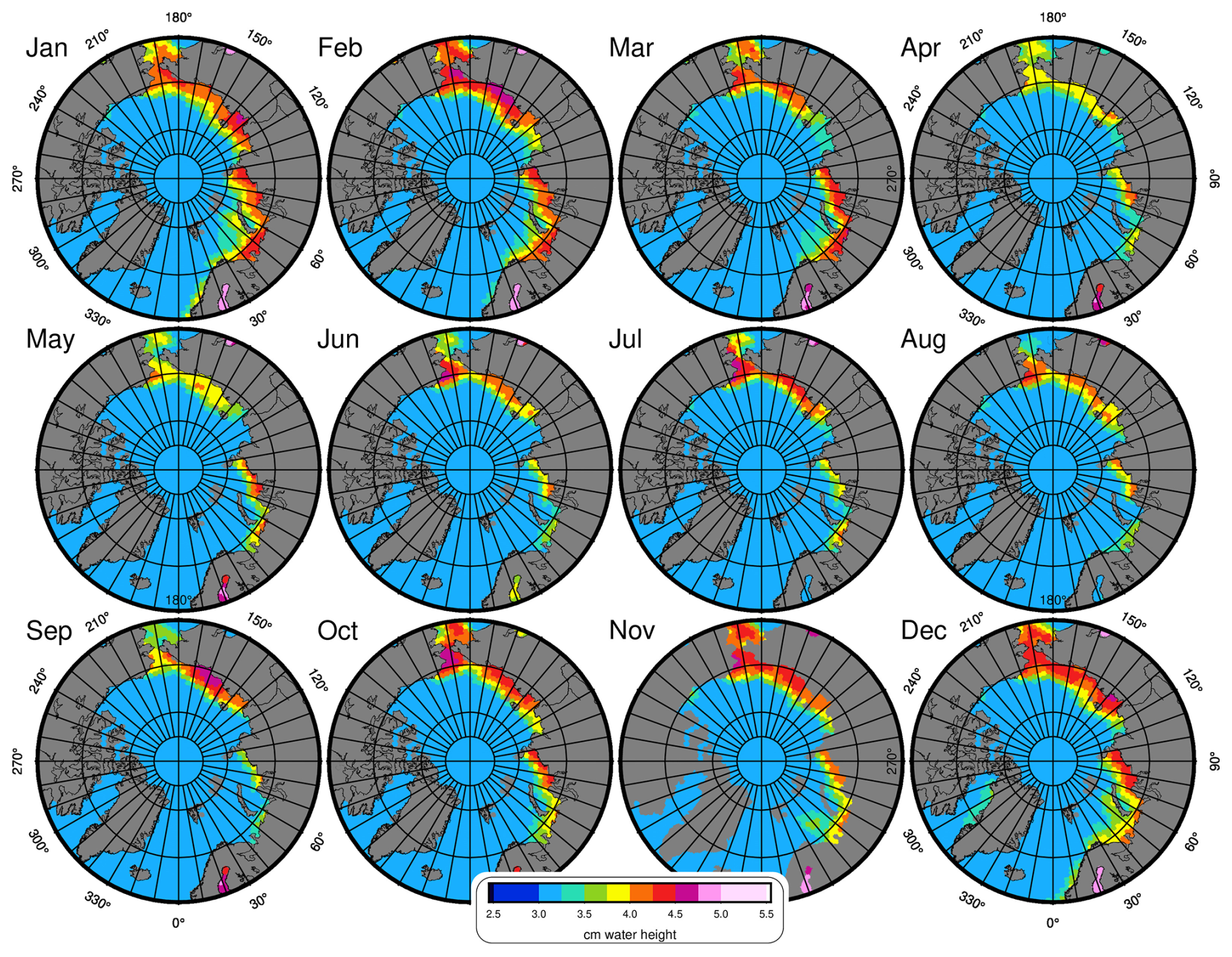
Figure A3 Arctic ocean climatology of CSR RL06.2DO constraint sigmas. The DO sigmas are not a strict climatology, but vary uniquely each month. Shown is the average value per month over the 2002–2024 series, which can be more easily compared to Figs. A1 and A2.

Appendix B: Comparison of barystatic-GRD series with the JPL and GravIS GRD estimates

Recently, two other barystatic-GRD series have been released. JPL's barystatic-GRD series (Landerer and Wiese, 2025) is based on their RL06.3 version 4 mascons with coastal resolution improvement (CRI) filter. The GravIS barystatic-GRD series (Dahle et al. 2025, Dobslaw et al., 2025) is based on the COST-G RL02 spherical harmonic series. Both barystatic-GRD series were made via the same mathematical theory as our DO mascon barystatic-GRD series, but use the JPL or COST-G land data to define the mass inputs. The GravIS barystatic-GRD series also allows the atmosphere to drive their barystatic-GRD response, which the DO and JPL mascon barystatic-GRD estimates do not.

Directly subtracting the barystatic-GRD files is not recommended, since the JPL output as defined is smoothly spread across $\mathrm{1}/\mathrm{2}$° × $\mathrm{1}/\mathrm{2}$° grids and the GravIS output is given on 1° × 1° grids, while the DOM barystatic-GRD is averaged over the larger CSR mascons. However, the three barystatic-GRD series' trend, annual amplitude, and annual phase maps (Figs. B1–B3) can be directly compared. Additionally, the ocean-averaged timeseries over the CSR mascon ocean mask (Fig. B4) can be fairly compared between the series.

The DO mascon and JPL barystatic-GRD estimates are very similar in overall shape and have nearly identical annual phases, when averaged over the global oceans. The JPL barystatic-GRD estimate has a slightly higher trend (0.203 cm yr⁻¹ compared to 0.193 cm yr⁻¹) and a slightly lower globally-averaged annual amplitude overall (0.87 cm vs 0.93 cm). These differences (0.01 cm yr⁻¹ in trend and 0.06 cm in annual amplitude) do not define an error estimate of the barystatic-GRD method itself, but are a reflection of the level of difference between the JPL and CSR mass estimates over land.

The GravIS barystatic-GRD series is markedly different from either the DO or JPL mascon barystatic-GRD series. GravIS mapped trends (Fig. B2) are generally smaller, leading to an ocean-averaged trend (Fig. B4) of only 0.121 cm yr⁻¹, considerably lower than the DO (0.193 cm yr⁻¹) and JPL mascon (0.203 cm yr⁻¹) trends. The use of spherical harmonics, which lose some of their coastal land/ice signal into ocean grids as leakage, may explain some of this difference. The annual amplitude of the globally-averaged GravIS barystatic-GRD series (0.877 cm) is of similar those of the DO and JPL series. Inclusion of the atmospheric forcing leads to higher annual amplitudes around Eurasia. However, even given this additional forcing, the differences appear larger than we might expect from the results of Tamisiea et al. (2010).

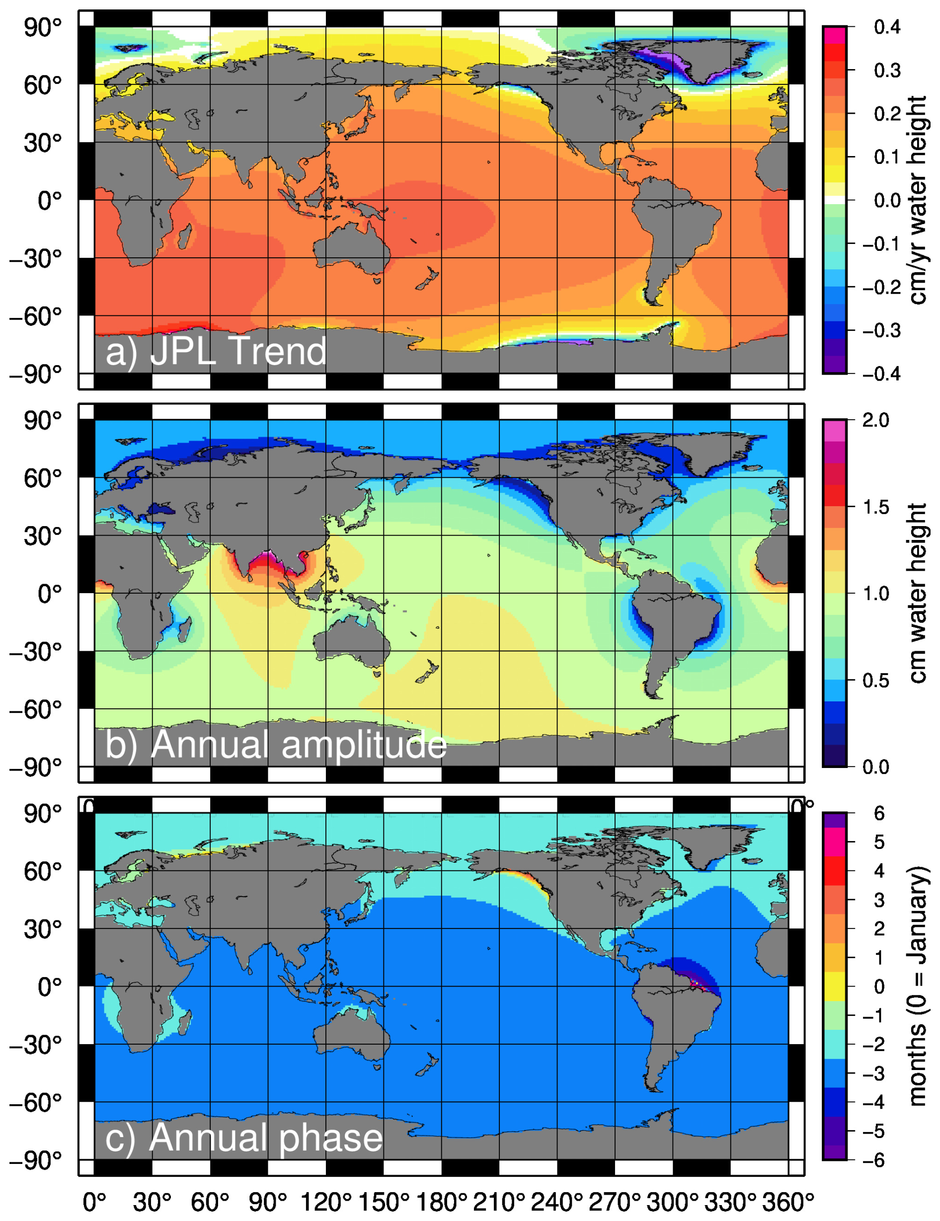
Figure B1 The linear trend (a), annual amplitude (b), and annual phase (c) of the JPL barystatic-GRD estimate. The ocean mask used was the CSR mascon mask (to $\mathrm{1}/\mathrm{2}$° resolution). Phases in (c) are defined such that 0 refers to an annual maximum in January, and ± 6 refers to a maximum in July.

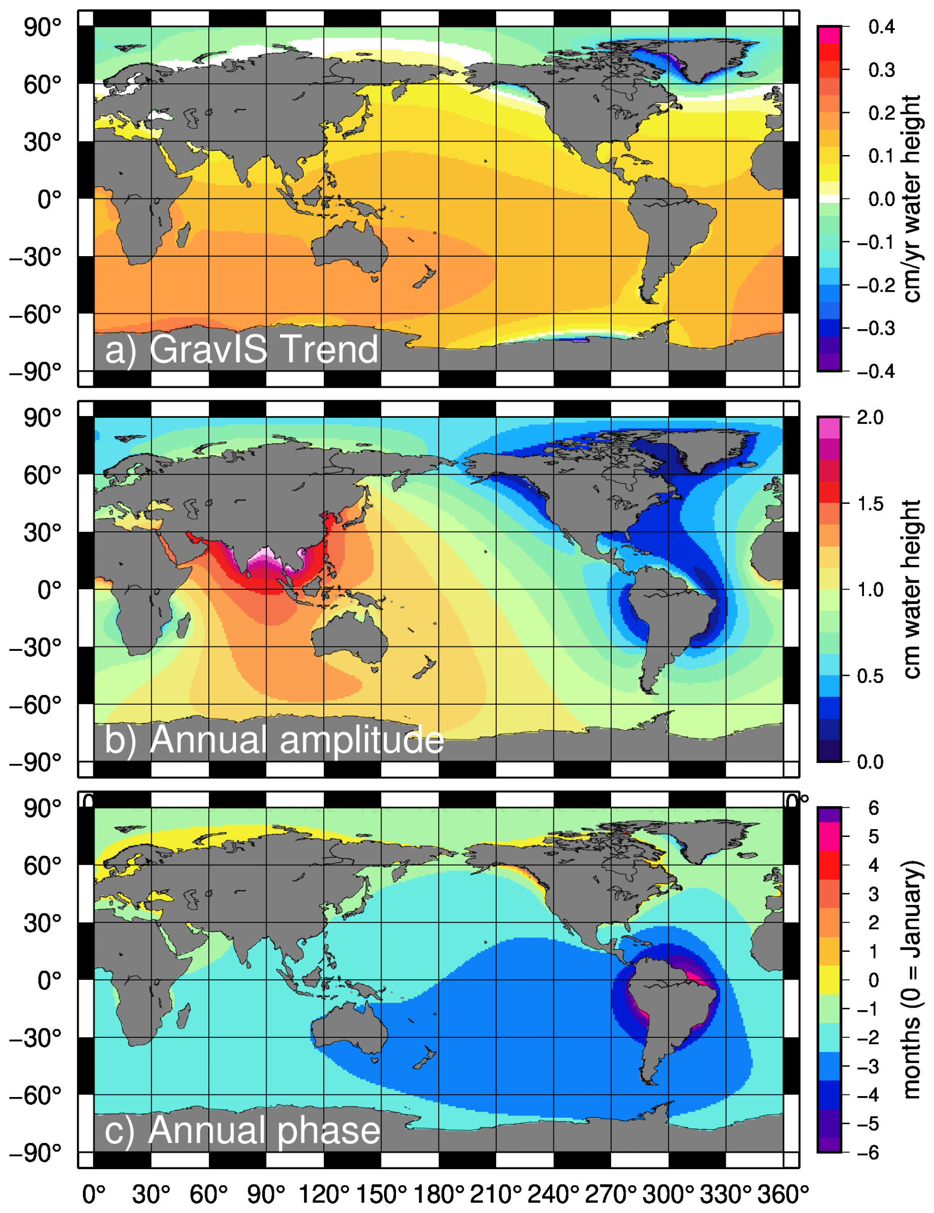
Figure B2 The linear trend (a), annual amplitude (b), and annual phase (c) of the GravIS barystatic-GRD estimate. The ocean mask used was the CSR mascon mask (to 1° resolution). Phases in (c) are defined such that 0 refers to an annual maximum in January, and ± 6 refers to a maximum in July.

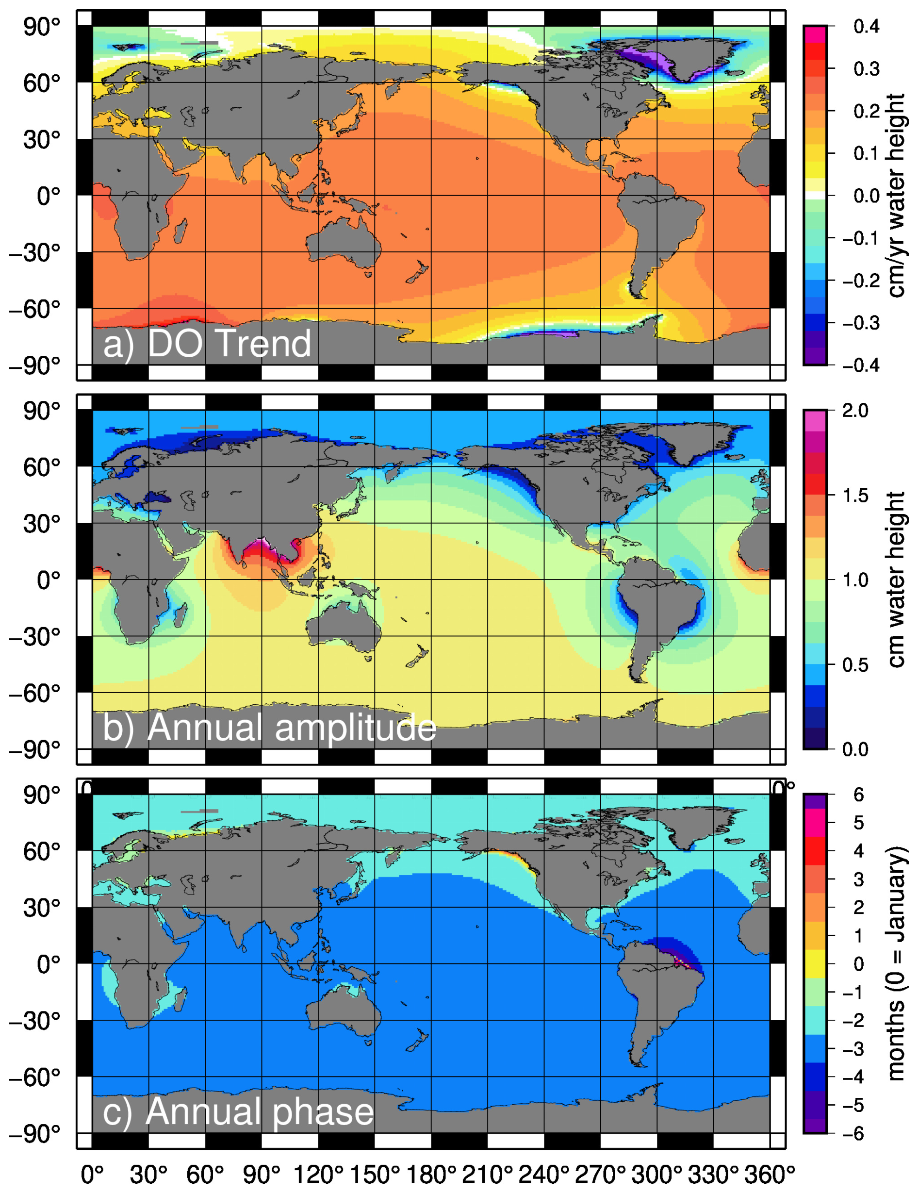
Figure B3 The linear trend (a), annual amplitude (b), and annual phase (c) of the DO mascon barystatic-GRD estimate. The trend and annual amplitude are identical to those shown in Fig. 7, and are repeated here for ease of comparison. Phases in (c) are defined such that 0 refers to an annual maximum in January, and ± 6 refers to a maximum in July.

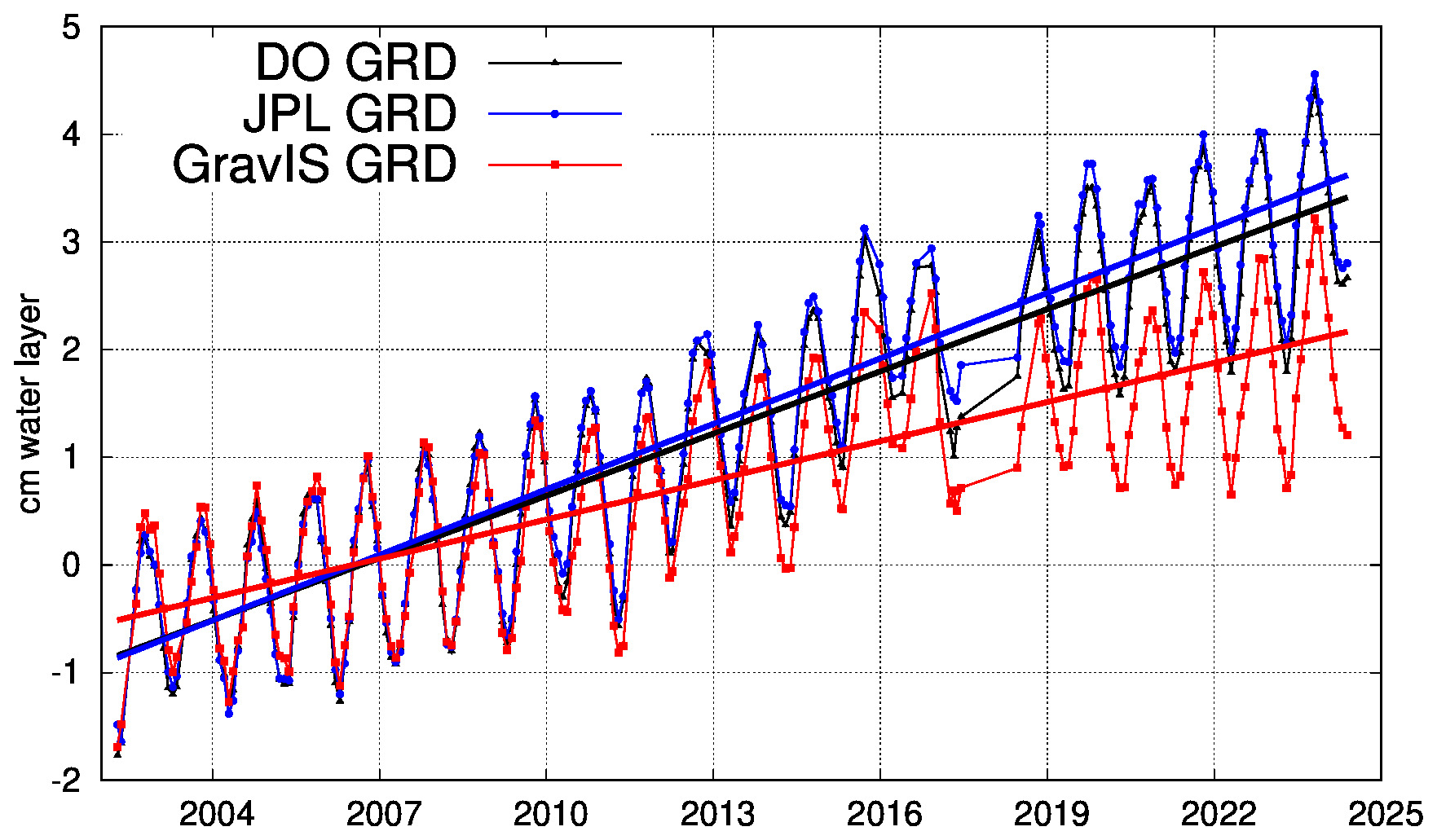
Figure B4 The mean signal over the global oceans (as defined by the CSR mascon mask), for the barystatic-GRD estimates from the new DO mascons, the JPL mascons, and the COST-G GravIS spherical harmonics.

Appendix C: Comparison of DOM and CSR RL06.3 with ECCO

In an attempt to estimate an uncertainty for our DO mascons, we difference them from the ECCOv4r4 data, and compare that result to a similar difference with ECCO using the standard CSR RL06.3 mascons (Fig. C1). We generally assume that greater similarity with ECCO implies an improvement (though it is always possible that ECCO is missing signal that GRACE might be correctly seeing). As before, we bear in mind that the JPL GRACE RL05 mascons were used as one of the assimilated datasets during the ECCOv4r4 processing. However, we do not anticipate this benefitting the DO mascons over the CSR RL06.3 mascons or vice versa, and as such we hope this metric will prove insensitive to any sway the assimilation of GRACE may have had on ECCO. To make a fair comparison, we again remove the area-weighted mean from the ocean each month from ECCO, since that was added artificially. We do the same with the comparison RL06.3 mascons, but not with the DO mascons because those already have a true barystatic-GRD series removed.

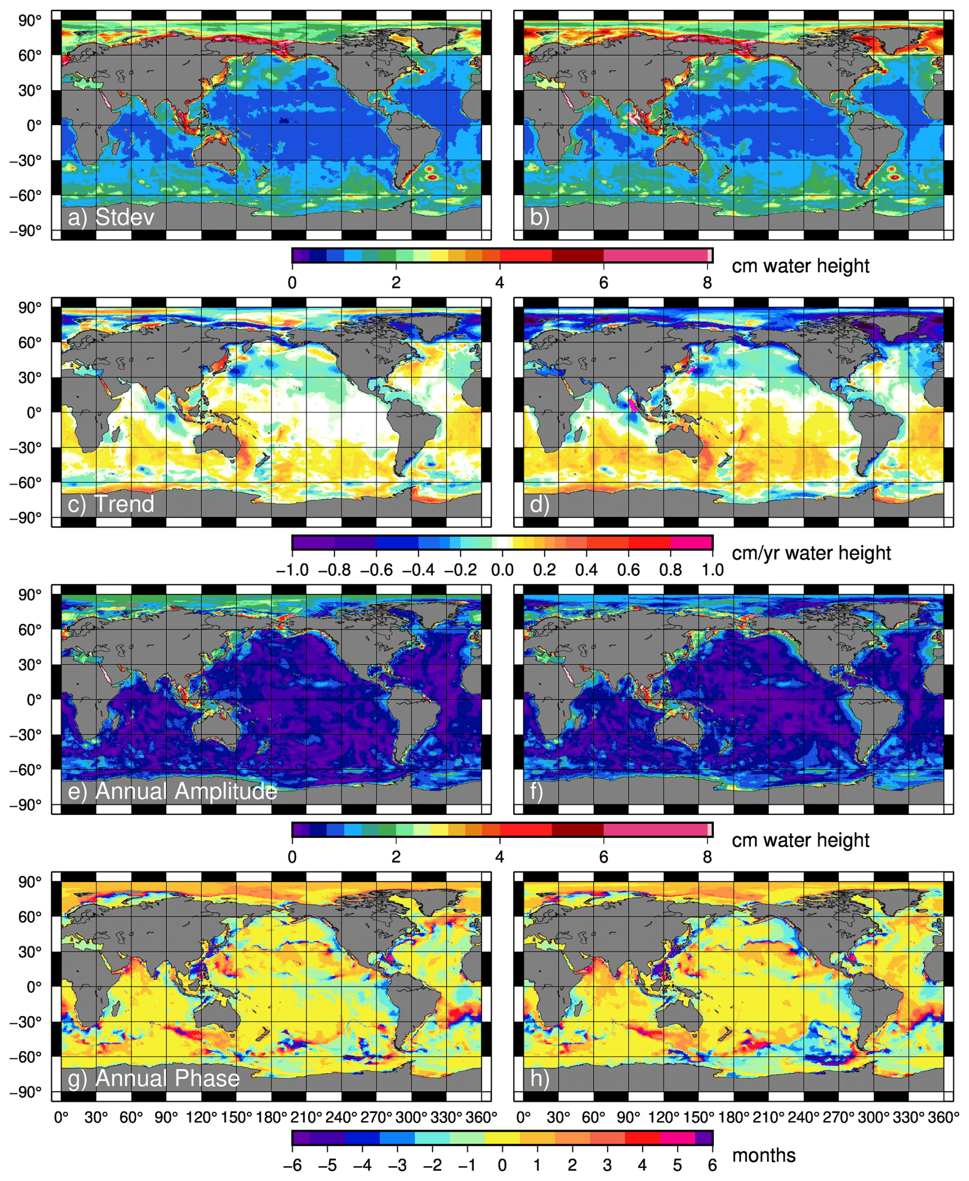
Figure C1 The differences between the DO mascons and ECCOv4r4 (left) compared to the difference between the CSR RL06.3 mascons and ECCOv4r4 (right), for the following statistics: standard deviation (a, d), linear trend (b, e), annual amplitude (c, f), and phase of the annual signal (d, g). The phase difference is given in months relative to the respective GRACE mascon annual phase.