Long-term sea surface temperature time series from Malin Head, Ireland

A 67-year, ongoing Sea Surface Temperature time series from Malin Head, in the north of Ireland, has been developed from data collected by Met Éireann and the Marine Institute. Over the course of the time-series, multiple measurement methodologies, sampling frequencies, and sub-site positions have been used for different periods. Resulting from this, two separate datasets have been created and publicised for usage, the quality controlled full-resolution measurement dataset (https://doi.org/10.20393/85D35444-2FB3-4791-A977-AE29BB3B3CFC, Marine Institute, 2025b), and a standardised daily average dataset (https://doi.org/10.20393/314DE8E2-79F0-4D36-B2BE-EE2A7E5590E2 Marine Institute, 2025a), the latter of which has undergone various processing steps, including removal of a diurnal signal. The standardised dataset creates and will continue a valuable, longstanding continuous time series which allows for more simplified long-term trend analysis compared with observation collections, which differ in measurement types and frequencies. The Malin Head sea surface temperature data, alongside a co-located tide gauge dataset are instrumental in understanding coastal ocean climate change in the region. Both datasets included are made available through the Marine Institute's Data Catalogue, have been assigned DOIs, and are made available from the Marine Institute's ERDDAP service.

1 Introduction

Observations and in-situ measurements underpin our scientific understanding of the Earth and how its environment functions, and are the basis on which modelling has been developed. While individual or short-term measurements can be useful in some applications, long-term measurements are the most informative in understanding the Earth's systems and how they evolve and change over time (Acquaotta and Fratianni, 2014). On a global scale, there are a relatively small number of long-term datasets measuring oceanographic conditions when compared to those measuring physical conditions in the terrestrial or atmospheric sphere (Luterbacher et al., 2024). This can be associated with a mass funding loss in the late 1980s, which cut off many monitoring projects with decades of data at the time (Duarte et al., 1992), as well as the fact that oceanographic monitoring can be more labour intensive and weather dependent. Due to the relative rarity of these time series, the importance of their continuation, publication and wider accessibility cannot be overstated (Luterbacher et al., 2024).

In terms of Sea Surface Temperature (SST), this variable gives insight not only into oceanic conditions but contains a more coupled relationship, which provides some understanding of atmospheric conditions as well. It can help to elucidate changes in the ecological structuring of a region (e.g. Sailley et al., 2025), to help separate trends of natural variability from anthropogenic change (e.g. Poul et al., 2025), and is utilised to help model future climate scenarios (e.g. Vytla et al., 2025).

Malin Head

Malin Head, in County Donegal, is the most northerly point on the island of Ireland. This longstanding time series, traditionally known as “Malin Head” is located 2.4 km from Malin Head on Portmore Pier, a working pier located in a small bay, which is open to the Malin Sea to the northeast (Fig. 1).

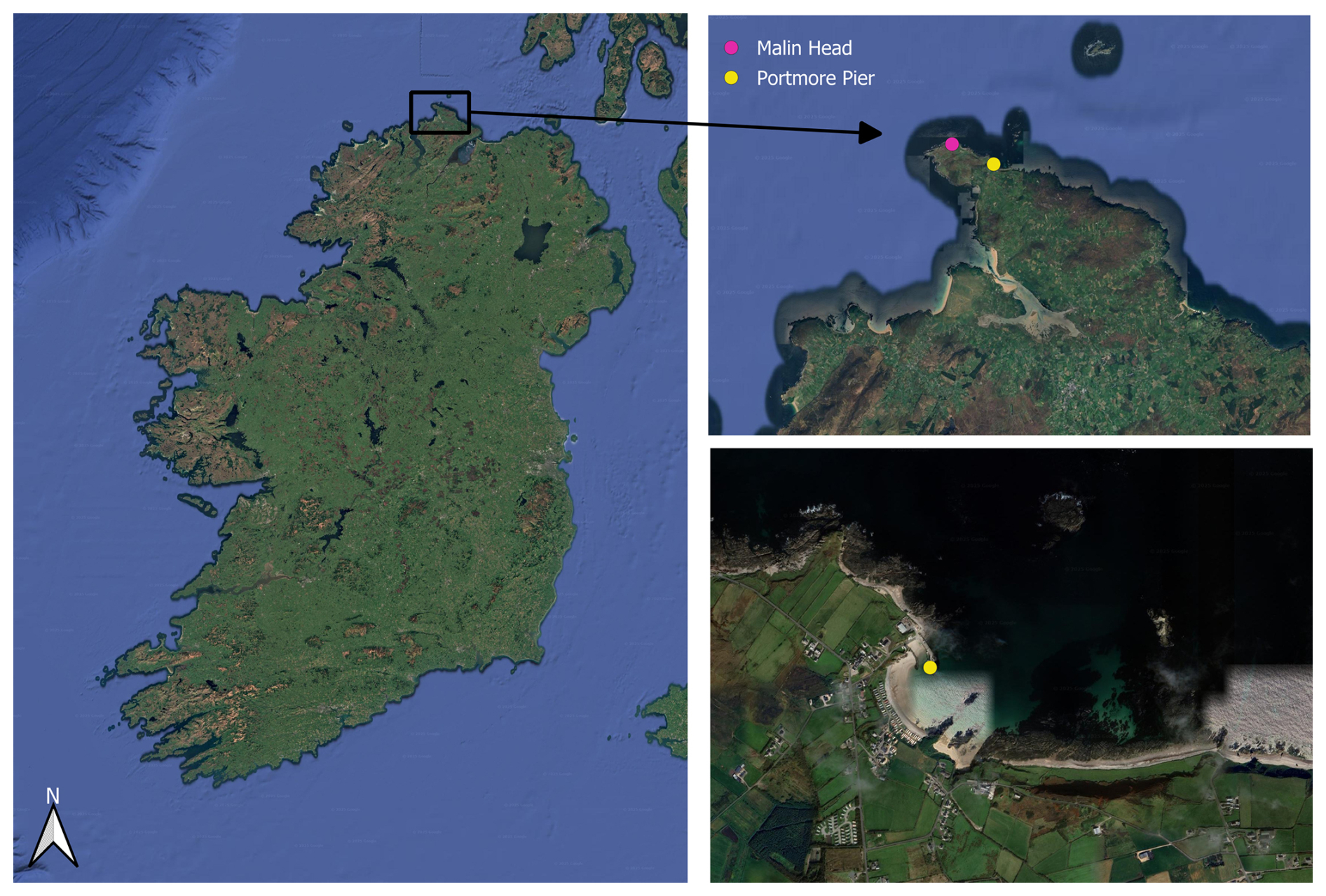
Figure 1 Map showing the locations of Malin Head (pink) and Portmore Pier (yellow) (Background map extracted from © 2025 Google: © Landsat/Copernicus, © IBCAO, © Data SIO, NOAA, U.S. Navy, NGA, GEBCO, © Airbus).

Malin Head is an important site in Ireland because it is the primary ordnance datum (OD) used for mapping and surveying across the island of Ireland. An OD is a vertical location used as the basis for deriving altitude for mapping services. OD Malin has been the Irish national datum since 1970 taken as the mean sea level from the tide gauge between 1960 and 1968 (Geological Survey Ireland, 2021).

Malin Head has been the location of a weather monitoring station since 1885. In 1955, the weather station moved to a location adjacent to Portmore Pier (55°22^′20^′′ N, 7°20^′20^′′ W). Sea surface temperature began to be collected as part of the weather station output from the pier in 1958.

While Malin Head is a coastal location and thus more highly influenced by atmospheric and anthropological variances than an open ocean site may be, the SSTs recorded there are important for understanding the coastal oceanography of the region. Surface waters surrounding Malin Head are impacted by coastal currents traversing clockwise around Ireland from the southeast of the island, around the west coast, and across the northern coast before proceeding further north towards Scotland (Raine and McMahon, 1998; Fernand et al., 2006). Furthermore, the larger Northeast Atlantic region, with the presence of larger scale currents, such as the North Atlantic Current, and the dual influence from the subpolar and subtropical gyres is key to understanding connectivity between open ocean and shelf/coastal seas in the area (Caesar et al., 2021; Daly et al., 2024). Additionally, the longevity of the time series allows for the separation of the small-scale variability, evident in a coastal region, from the underlying trends which permeate these regions of influence.

The full-resolution measured data collected at Malin Head are made accessible to the public and the data have also been curated into a standardised time series. Section 2 discusses the methodologies for collection of the measured data and the creation of the standardised time series from the measured data, Sect. 3 discusses the quality check procedures undertaken for the datasets and the error for each segment of the time series, Sect. 4 overviews usages for the datasets including warming trend analysis, and Sect. 5 maps where and how to access both standardised and measured datasets.

2 Data Curation

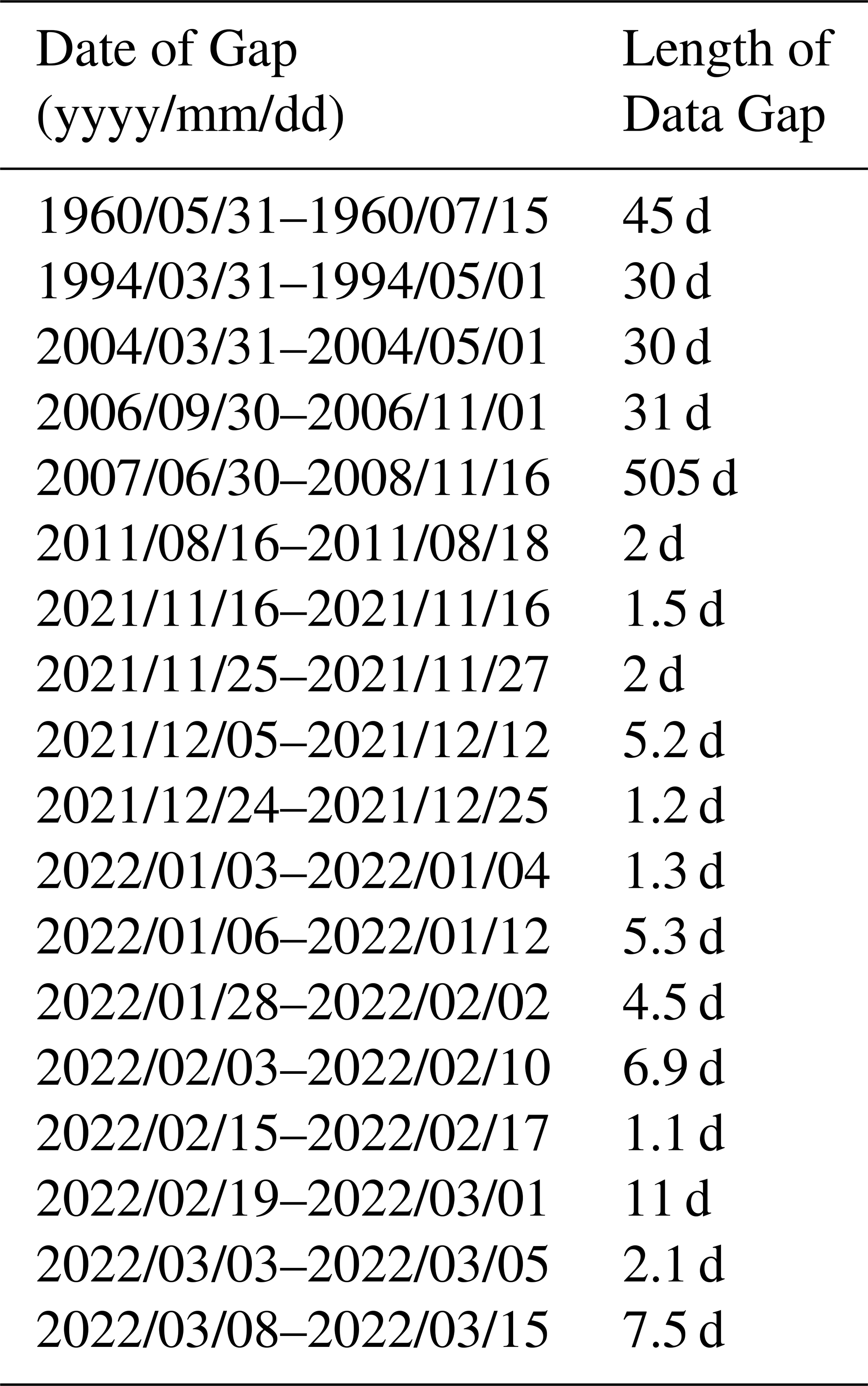
At Malin Head, there have been almost continuous measurements of SST since the beginning of 1958 (see Table 1 for an outline of the gaps within the time series). However, due to differing collection methods, sampling frequencies, and slightly different collection positions at the location, these measurements have been separated into three different segments.

Table 1 Gaps in SST data within the full-resolution dataset. A time difference is considered a gap if at least a full day of data is missing. Presence of bad data does not constitute a gap.

2.1 Segment 1 – Well Measurements

Met Éireann began twice-daily measurements of sea surface temperature on 1 January 1958 at Malin Head (Nolan et al., 2021). The first few months of data have been identified as bad and thus not included in the published datasets, so the datasets begin on 28 April 1958. These measurements were taken 2 m below the surface of a well on Portmore Pier. The well was connected by pipe to 30 m offshore of the pier (Cannaby and Hüsrevoğlu, 2009; Dunne et al., 2009). These twice-daily measurements continued until 31 March 1991.

2.2 Segment 2 – Bucket Measurements

On 1 April 1991, there was a transition from the twice-daily well measurements to once-daily measurements. These measurements were collected by either collecting a bucket of water from beside the pier and measuring the temperature from the bucket or by directly lowering an electronic temperature sensor into the water from Portmore Pier and reading the temperature value from it (Dunne et al., 2009). These measurements continued until 30 June 2007.

2.3 Segment 3 – Continuous Measurements

After a 17-month gap (see Table 1), the Marine Institute took over the time series and established long-term deployments of in-situ temperature loggers beginning on the 16th of November 2008 and these deployments have been continuous since then (Nolan et al., 2021). Seabird 39 (or 39plus) instruments are fixed to the pier 3 to 4 m below OD Malin. Measurements have been collected every 30 min continuously throughout this segment of the time series, excluding minor gaps between sensor deployments and due to occasional sensor issues (Table 1). From 2008–2012, there was a combination of pier locations chosen for sensor deployment (middle: 55.371480° N, 7.334372° W; and end: 55.371308° N, 7.334328° W). From 2012–2021, deployments included both mid- and end-pier deployments but the end-pier deployments are exclusively included in the standardised time series due to the location being less sheltered and diurnally impacted. Since 2022, two sensors have been deployed together at the end of the pier, to ensure a backup in case of sensor issues, and mid-pier deployments have ceased. Where there have been two sensors deployed for the same time period, after review of the data, a primary sensor has been chosen for inclusion within the publicised datasets.

2.4 Standardised Time Series

Each segment of observed temperature, although measured differently, can be treated as an individual time series from which a daily averaged product can be derived. However, the value of having a single daily averaged product across the entire 67 years of data has motivated the effort to merge these segments together, while accounting for the differences between them. Most of this work was carried out between 2017 and 2020 and is now finalised and made available as a combined data product.

The four main considerations when merging these segments are: Position and depth of measurement, tidal signal, diurnal signal and measurement bias. Due to the absence of any data on vertical variation in the water column, adjustments could not be made for the difference in depths of measurements, being fixed from the sea surface in Segments 1 and 2, and fixed relative to the sea floor in Segment 3. Tidal signal analysis was performed on all segments using UTide (a Matlab toolbox; Codiga, 2011), which showed no significant tidal effect and only highlighted the annual cycle. Adjustments were applied to Segments 1 and 2 based on analysis of the modern, high-resolution Segment 3. These adjustments account for diurnal signal and in Segment 2 for measurement bias. Adjusting for both was considered the best approach to account for the different positions and measurement methods of the two older segments. Segment 2, having only one sample per day at various times and sampled inside the shelter of the pier, most required the removal of a diurnal signal. Segment 1, being connected to open water and having two samples per day to average over, less required diurnal signal removal. Measurement bias calculation was also possible between the bucket method of Segment 2 and the modern sensor method of Segment 3, due to the proximity of measurements and the results of a bucket experiment in 2010 that ran for five months concurrent with Segment 3 sampling. Due to a smaller diurnal signal and lack of contemporaneous data between Segment 1 and 3, no measurement bias was calculated or applied to Segment 1.

The following sub-sections detail the methodology and required adjustments made for diurnal signal and measurement bias to the earlier segments, before presenting this combined/standardised temperature time series data product.

2.4.1 Daily averages

Before calculating daily averages, the modern-day Segment 3 data from 2008–2020 was used to derive a diurnal signal. This involved pre-organising data from each sensor deployment and included interpolating over occasional one-hour gaps in the data for years: 2011, 2012, 2016, 2018, 2019, 2020 (all other years had no gaps). Then a smoothed dataset was derived using a 49 point (24.5 h) running window convolution, which allows for the removal of diurnal signal, while longer-term trends, like seasonality, are retained. The convolution method was chosen over standard filtering, as filtering introduces a delay. The smoothed dataset is then subtracted from the original temperature dataset to reveal a diurnal signal, as previously applied to oceanic pCO₂ (e.g. Leinweber et al., 2009; Thomas et al., 2012). This method was then successfully validated by performing the exercise again but on a dataset that had the diurnal signal already removed. Validation results showed no significant signal, only random error at amplitudes an order of magnitude smaller than the diurnal signal.

Segment 3 daily averages were computed as the mean of all values per day from the smoothed dataset. This removes the diurnal signal, and in doing so, removes any diurnal ambiguity between mid and end pier locations and provides consistency with Segments 2 and 1 described next.

The full time series of diurnal signal (observed less smoothed) is then averaged, per hour, per month, in preparation for removal from Segments 1 and 2. This resulting mean signal displays a strong diurnal cycle in the warmer months (March–October) with minimum temperatures occurring between 06:00 and 08:59 UTC, while the colder months' diurnal cycle had a lower amplitude and minimum temperatures between 00:00 and 02:59 UTC. The full set of mean diurnal signals can be seen in Table S1 in the Supplement, while monthly (June) and hourly (16:00) examples can be seen in Fig. 2a and b respectively.

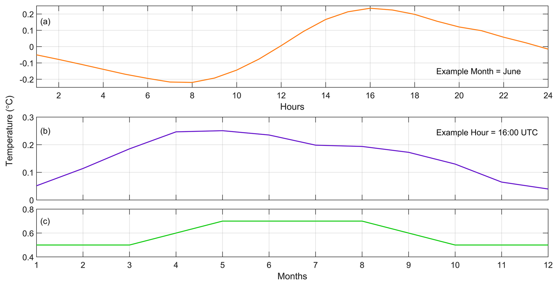
Figure 2 Correction Curves. Example diurnal signals for the month of June (a) and for the hour of 16:00 UTC (b) display the values removed from Segment 2 for that example month and hour. See Supplementary Table S1 for the entire set of mean diurnal signal values. The derived measurement bias curve on Segment 2 is displayed in panel (c).

The Segment 2 temperature time series, having one measurement per day, has the diurnal signal subtracted to produce a single normalised or “daily averaged” value. For Segment 1, an attempt was made to calculate a mean monthly diurnal signal by subtracting a daily mean running average. This method produced a smaller diurnal signal, likely due to its connection with open water, but the method was considered unreliable due to Segment 1 only having two samples per day. The decision was made to use the mean diurnal signal, derived from Segment 3, but to dampen it by half before removal from Segment 1. Once all values were diurnally corrected, they were averaged per day to produce a daily averaged value for the segment 1 dataset.

2.4.2 Measurement Bias

An exercise in 2010 (July–November) to compare bucket measurements with the seabird temperature sensors highlighted a warm bias in the bucket measurements relative to the sensor. As the bucket experiment was only five months long, a more comprehensive analysis was required. By comparing monthly averages from Segment 2 (January 2000–June 2007) with Segment 3 (2008–2020) an annual bias curve was calculated. This curve had three outliers, where June was exceptionally high and October and November were low. It was decided to (a) combine this curve with the five-month bucket results, (b) to smooth the curve (three month running average), and (c) to round to one decimal place, thus creating a reasonable sinusoidal curve to be applied to correct for measurement bias in Segment 2 (see resulting correction curve in Fig. 2c).

Measurement bias was also investigated between the Segment 3 mid and end-pier locations, through examination of a 14-month contemporaneous dataset (November 2015–February 2017). This showed that the mean difference in the smoothed data (i.e. the diurnal signal removed) from end-pier to mid-pier is −0.05 °C (mid-pier cooler), with a RMSE of 0.11. Morning only values (06:00–08:59 UTC) of smoothed data show no difference between mid and end pier locations (to 4th decimal place). Although the difference is small, it must be considered, due to the standardised dataset relying on mid-pier measurements for periods of Segment 3. Given the correction would only be 0.05, a decision was made that there was no solid basis for adding any correction to the mid-pier data when adding it to the standardised daily time series, though it is important to recognise this as a limitation.

2.4.3 Segment Combination

Once all adjustments were made, the daily average time series was combined from all segments, uploaded to the Marine Institute SQL database and published on ERDDAP. On receipt of new sensor data annually (usually around February) from the Malin Head site, Marine Institute data stewards will compute that previous year's daily averages and append to the existing dataset.

3 Data Integrity

Data management is a keystone in data processing as it provides the framework to ensure that data is handled and stored the same way no matter who is dealing with it. At the Marine Institute, which is the Irish National Oceanographic Data Centre (NODC), data is managed through the creation and implementation of quality management framework (QMF) packs which are organised to focus on a specific project or type of sensor which collects data. The packs are comprised of a number of documents, which provide the background and structure for the collection, processing, and publishing of datasets, as well as process flow diagrams (e.g. Fig. 3), which allow for the visualisation of the steps for data processing. The data management through the QMF structure at the Marine Institute has been accredited under UNESCO's International Oceanographic Commission (IOC) IODE programme (IODE, 2025) and it holds CoreTrustSeal certification (CoreTrustSeal, 2025) as a trusted data repository for data management and preservation. The QMF packs are built to ensure adherence to the FAIR data principles (Findability, Accessibility, Interoperability, and Reusability) which make sure that data and metadata are handled adequately for potential future uses (Wilkinson et al., 2016). Another advantage of developing data process flows under the guidance of a quality management framework is that it lends well to disseminating and publishing not just the datasets, but the methodologies constructed to do so. A recent example is the Marine Institute's vessel CTD dataset and open source Jupyter Notebook toolbox for processing vessel CTD data, developed under the same framework as the Malin Head datasets (O'Sullivan et al., 2025).

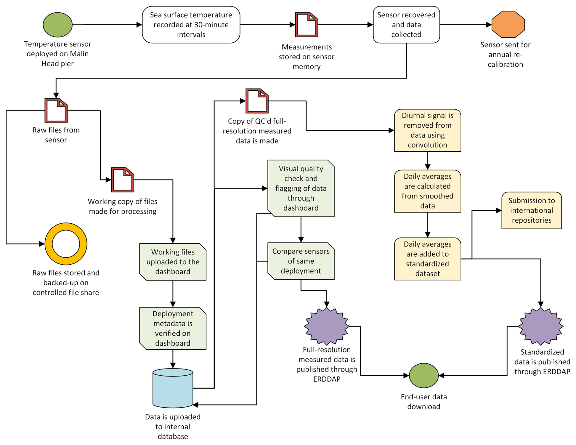
Figure 3 Process flow diagram for Malin Head data from sensor deployment to the download of data by the end-user. Green boxes denote steps that occur on the in-house dashboard developed for fixed CTD processing and quality control. Yellow boxes denote steps that only occur in the creation and publishing of the standardised dataset from the measured data.

3.1 Dashboard and Visual QC

A containerised online dashboard has been recently developed at the Marine Institute, on a Python platform, through which data files downloaded directly from instrument-specific software can be uploaded and archived to an SQL database, quality checked using automated routines (e.g. range checks and spike identification) and visual screening, and published publicly to the Marine Institute's ERDDAP data service. The advantage of using dashboards is in standardisation and streamlining of the data process flow from acquisition to publication of a wide array of environmental parameters and instrument make/models. This dashboard standardises data processing for all fixed CTD-DO datasets hosted by the Marine Institute. For the Malin Head data, which is temperature-only, the dashboard facilitates an automated gross range check (−5 to 40 °C) followed by visualisation and screening of the collected data. Visual screening of the SST data will identify and flag any remaining spot outliers and anomalous data, which are not the result of natural variation, but likely from sensor malfunction or error. When there are multiple sensors deployed together in the same location on the pier at Malin Head over the same period, they are also compared to each other to help differentiate natural variation from sensor issues. This comparison is also important in distinguishing which sensor will be utilised for the complete time series.

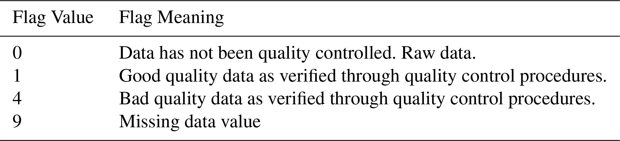
The Marine Institute's dashboard, database, and publishing server utilise the SeaDataNet's standards for data quality control (SeaDataNet, 2010) for the data flagging system (Table 2).

Table 2 Overview of the SeaDataNet quality control flags that are utilised in the Malin Head time series.

3.2 Uncertainty Analysis

When presenting a dataset such as the Malin Head SST product, uncertainty (combined system error, accuracy, sensitivity, drift etc.) is an important metric to consider with it. However, with the nature of the time series discussed, the ability to calculate uncertainties for the measurements is hampered by the lack of specification on instrumentation used for the first two segments of the time series. Without accurate information on what exact instrumentation was used for SST measurements for these periods of time it would be impossible to quantify a specific uncertainty value. For the first two segments, SST is reported to a tenth of a degree, so the error margin is at least ±0.1 °C. Both segments are modified for inclusion in the standardised dataset and thus the uncertainty of the reported temperatures will change accordingly.

For Segment 3, the SBE 39 and 39plus instruments report temperature with a resolution of 0.0001 °C. Seabird reports the accuracy of the SBE 39 instruments to a margin of ±0.002 °C and a drift of no more than 0.0002 °C monthly (Seabird, 2024). In order to minimize the effects of the drift in the instrumentation over time, sensors are sent to the Seabird factory for calibration annually between deployments. The maximum error on data points in the full-resolution dataset for Segment 3 would be ±0.0044 °C, which accounts for the instrument margin and up to a year of drift (deployment length for sensors) for each data point.

With the process taken to prepare Segment 3 data for inclusion in the standardised time series, the uncertainty introduced is minimized because the data points that could have been affected by edge errors during the convolution process are removed from the dataset. Errors on data points do change through the process of convolution and in creation of the daily averages and thus must be accounted for. Each data point which is output from the convolution has an error value associated with the combined errors which are used in the window for convolution (Eq. 1). This post-convolution error can be estimated at ±0.0006 °C for each point. After convolution, the resultant data points are averaged over the span of a day and the propagation of error associated with this is summarized in Eq. (2). The resultant daily averages for Segment 3, which are included within the standardised data product, would have an error of ±0.00009 °C, which is significantly lower than the instrument error for the full-resolution dataset.

$$\begin{array}{}\text{(1)}& {\displaystyle }{\mathit{\sigma }}_{\mathrm{c}}={\displaystyle \frac{\sqrt{\mathrm{49}\cdot {\mathit{\sigma }}_{\mathrm{i}}^{\mathrm{2}}}}{\mathrm{49}}}\text{(2)}& {\displaystyle }{\mathit{\sigma }}_{\mathrm{t}}={\displaystyle \frac{\sqrt{\mathrm{48}\cdot {\mathit{\sigma }}_{\mathrm{c}}^{\mathrm{2}}}}{\mathrm{48}}}\end{array}$$

Where σ_i is the maximum instrument error for a data point, σ_c is the error resultant from convolution, and σ_t is the total error on standardised Segment 3 data points after making the daily averages.

Convolution using a 49-point window is also used in the creation of the normalised diurnal signal which is used to remove the diurnal signal from the data points in Segment 1 and 2, in order to prepare them for inclusion in the standardised time series. Adding or subtracting the normalised diurnal signal value from the original data points (with an error of ±0.1 °C) would result in normalized values with an uncertainty of essentially ±0.1 °C as the incoming error from the convolution is so much lower than the instrument error. Since the two daily values in Segment 1 are furthermore averaged, the final average uncertainties for Segment 1 data would be ±0.0707 °C in the standardised time series, which is lower than the instrument error for this segment, due to the use of the higher resolution Segment 3 data. The Segment 2 bucket data is also adjusted to be more similar to Segment 3 data after the diurnal signal has been removed (for full detail see Sect. 2.4). After the processing used for this adjustment, the average uncertainty for Segment 2 data is approximately ±0.1004 °C when it is included in the standardised data set (this does not account for changes in error from manual adjustments to account for anomalous data, but these were intended to decrease error within the dataset).

4 Data Application

4.1 Warming Trends

The complete SST time series from Malin Head is currently 67 years old. This longevity allows for analysis of the warming trend evident in the data beneath the seasonal components. There are many ways to evaluate warming trends in data. The easiest method is creating annual means for the data from which the warming trends can be analysed without removing seasonality. Using the standardised dataset, an annual mean was created by averaging all the daily data for each year, provided that each year had at least 11 months of data, and each month had at least 20 d of data. These criteria ensure that there is enough data to be truly representative of the year as a whole. With these criteria, only the years 1958, 1960, 2007, 2008, and 2022 are removed from the trend analysis due to lack of adequate data. Using this method for analysing a warming trend, the annual warming for the standardised data over the period 1959 to 2024 is 0.015 °C a⁻¹ (R²= 0.349) with a total warming for the period of 0.997 °C (Fig. 4b). When the same analysis is done for the measured dataset, which includes data for 2022 as it fits the requirements in this dataset, the annual warming trend is 0.019 °C a⁻¹ (R²= 0.412) with a total warming between 1959 and 2025 of 1.27 °C (Fig. 4a). The difference between the two resulting sets of values reported is due to the exclusion of 2022 data and an adjusted segment 2 in the standardised dataset analysis.

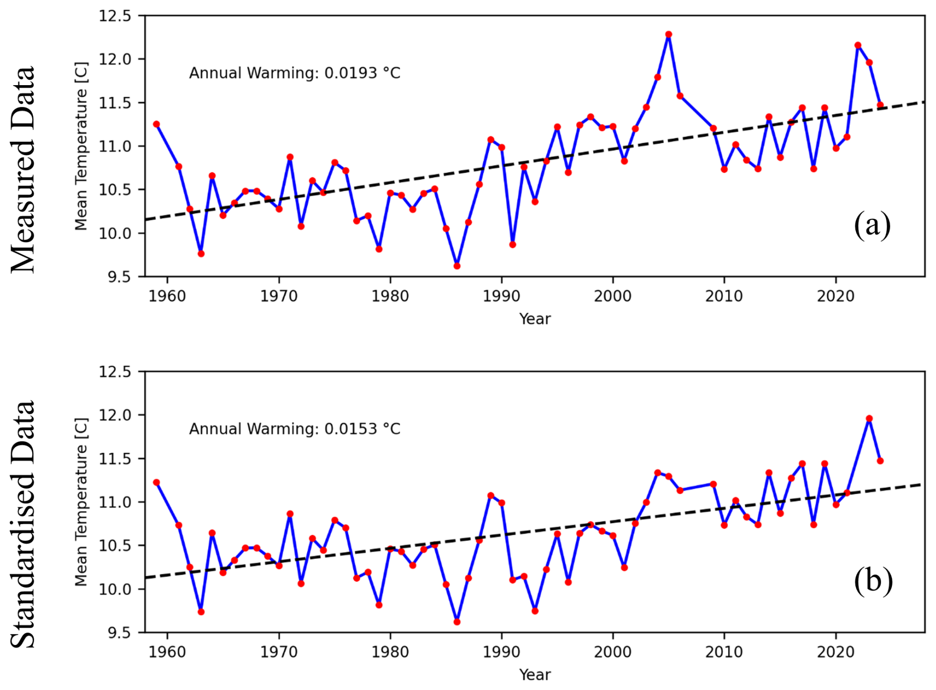
Figure 4 Warming trend analysis at Malin Head, based on annual temperatures from both the full-resolution measured data (a) and the standardised data (b).

Another way to analyse warming trends is through a separation of the seasonal components of temperature data from the underlying trend. In the open-source Python module statsmodels there is a built-in function seasonal_decompose() which separates the trend, seasonality, and residuals from given data with a defined period (Seabold et al., 2010). It estimates the trend using a convolution for rolling averages, removes the trend from the data, then the average for the given period is returned as the seasonal component. Using this function, the trend can be evaluated based off daily averaged data from the standardised dataset. For consistency with the annual mean trend, only data that fit the criteria for that method were used for this analysis. The resultant trend for the standardised data for the period 1958–2024 was evaluated as 0.016 °C a⁻¹ (R²= 0.359) annually, and 1.08 °C of warming for the whole period (Fig. 5b). When the measured dataset is used, the resultant warming trend comes to 0.02 °C (R²= 0.473) annually over the period, and 1.35 °C of warming for the whole period (Fig. 5a).

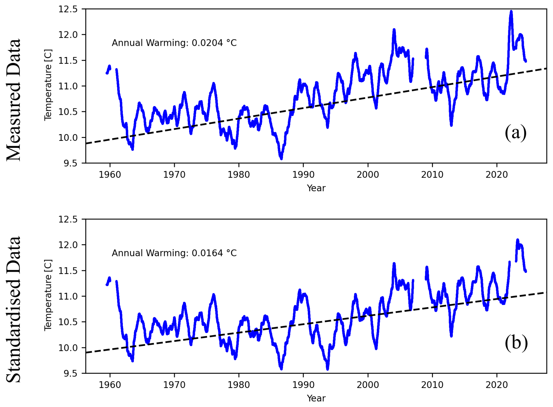
Figure 5 Warming trend analysis at Malin Head, using a seasonal decomposition function, based on daily-averaged data for both the full-resolution measured dataset (a) and the standardised dataset (b).

When looking at the patterns found in SST over time it is clear to see that warming has not been a steady or consistent rise from the beginning of the time series. While there is temperature variation from the beginning of the time series, annual average temperatures began to warm significantly in the 1990s through the early 2000s (Fig. 6). The warming undergone during this period accounts for a significant portion of the total warming at Malin Head throughout the length of the time series. When the period 1991 to 2005 is separated and the trend from annual mean values is calculated, the annual warming from the standardised data is approximately 0.085 °C a⁻¹ (R²= 0.694) and the total warming for the period is estimated to 1.19 °C, which is higher than the estimation for the whole period. The same trend can be seen in the measured data with annual warming for this period at 0.107 °C a⁻¹ (R²= 0.690) with a total warming from 1991–2005 of 1.49 °C. Cannaby and Hüsrevoğlu (2009) discussed this excess warming occurring around Ireland in the 1990s, where they analysed that the warming signal for this period could be almost evenly attributed to anthropogenic impacts and natural climate oscillations. They also discussed that the warming signal from anthropogenic sources would continue to grow over time. When annual SST anomalies are visualised based on the 1991–2020 average (Fig. 6), recent warming of the Malin Head site is apparent. For example, in the standardised dataset (Fig. 6b), there is a clear positive trend above the baseline since 2002 which can be contrasted with the previous cooler period. Furthermore, the two most recent years of data, 2023 and 2024, are also the two warmest years on record. The strong warm period is also clearly evident in the measured data (Fig. 6a)

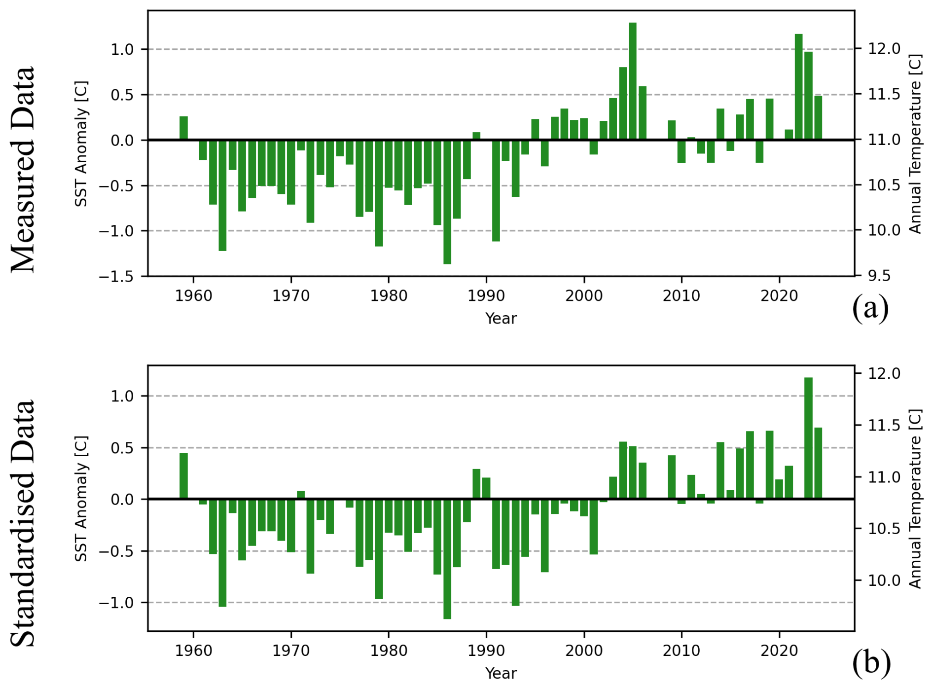
Figure 6 Annual mean temperature anomalies based on the 1991–2020 average, the current WMO climatological standard normal (WMO, 2017), for both the full-resolution measured data (a) and the standardised data (b).

4.2 Utilisation of Data in Published Work

Along with evaluating the long-term warming trend at Malin Head, this SST dataset has been utilised in a range of published works which demonstrate numerous use-cases for the data. The following outlines some of the ways the dataset has been leveraged in published works to date:

• Understanding the impacts of climate change (Cornes et al., 2023; Dye et al., 2013).

• Modelling environments and future outcomes (Holt et al., 2012; Tinker et al., 2018).

• Evaluating the causes of warming trends in the north Atlantic (Cannaby and Hüsrevoğlu, 2009).

• Understanding the effects of increasing SST on sublittoral communities (Goodwin et al., 2013).

• Describing the regional oceanographic setting and integrating with similar datasets to catalogue the most recent ocean climate conditions over the Northwest European Shelf (Gonzalez-Pola et al., 2023).

5 Data availability

The full-resolution measured dataset (https://doi.org/10.20393/85D35444-2FB3-4791-A977-AE29BB3B3CFC, Marine Institute, 2025b) is published in a few locations to ensure its accessibility to the public. The quality checked measured data at full-resolution is available for visualising or download through the Marine Institute's ERDDAP data server (https://erddap.marine.ie/erddap/tabledap/climate_malin.html, last access: 9 September 2025). Through this portal, users have the opportunity to filter the data using QC flags (as outlined in Table 2), specific dates, specific sensors, and additional variables. While this portal includes some metadata for the dataset, full metadata, including updates, are available on the Marine Institute's Data Catalogue entry (https://data.marine.ie/geonetwork/srv/eng/catalog.search#/metadata/ie.marine.data:dataset.4454, last access: 9 September 2025).

The standardised daily averaged data product (https://doi.org/10.20393/314DE8E2-79F0-4D36-B2BE-EE2A7E5590E2, Marine Institute, 2025a) is available separately on the same platforms and data servers (ERDDAP: https://erddap.marine.ie/erddap/tabledap/climate_malin_daily_average.html, last access: 9 September 2025, Data Catalogue: https://data.marine.ie/geonetwork/srv/eng/catalog.search#/metadata/ie.marine.data:dataset.5327, last access: 9 September 2025). This dataset is also submitted to the ICES Report on Ocean Climate (IROC) (Gonzalez-Pola et al., 2023; https://ocean.ices.dk/core/iroc, last access: 24 December 2025) where it is publicly available. Publishing to IROC was one of the first repositories where this time series was made available to the public and has been a key provider for increasing the visibility of the data on a global scale.

While the primary set of measured values and the standardised daily values are made available through ERDDAP, ancillary data, such as secondary sensors from segment 3, or the five-month bucket experiment in 2010, are also made freely available through the Marine Institute's data request service (https://www.marine.ie/data-request, last access: 9 September 2025). Ancillary data have been kept separate from the main dataset for simplicity and increased user accessibility.

Another co-located time series dataset that runs concurrent to the Malin Head SST time series is from the Tide Gauge located on Portmore Pier (2008 to present; ERDDAP: https://erddap.marine.ie/erddap/tabledap/IrishNationalTideGaugeNetwork.html, last access: 9 September 2025, Data Catalogue: https://data.marine.ie/geonetwork/srv/eng/catalog.search#/metadata/ie.marine.data:dataset.5277, last access: 9 September 2025). As part of the Irish National Tide Gauge Network (IN-TGN) this maturing set of sea-level data goes hand-in-hand with SST when investigating long-term change in the region.

6 Conclusion

Measurements of sea surface temperature have persisted at a pier near Malin Head, Ireland on an almost continuous basis since 1958. The resultant data has been made available to the public in both its full-resolution measured format as well as a standardised daily averaged time series. The process for the creation of the daily averaged time series required different steps for the different segments based on acquisition methods, instrumentation and frequency of measurement. Where scientifically reasonable, the early data was adjusted to be more continuous with the data collected from modern instrumentation. The daily-averaged time series has also been submitted to ICES to increase its visibility on a global scale.

These datasets have been used for multiple applications in the past and have many applications for future research and model integration or validation. Furthermore, using these datasets, a warming trend analysis was conducted for Malin Head that showed a 0.015–0.022 °C annual warming trend for the length of the study. The stronger warming trend from the full-resolution measured dataset when compared to the standardised dataset could be due to the lack of adjustments to Segment 2 (1991–2007) data and potentially the ability to include 2022 data in the analysis. The longevity of this time series is key to its relevance and so, in understanding the value of continuous time series, the Marine Institute has been developing similar long-term datasets in multiple other locations (e.g. Ballycotton: https://erddap.marine.ie/erddap/tabledap/climate_ballycotton.html, last access: 9 September 2025) which are quickly reaching a mature level. These ongoing time-series will receive continued support to allow them to grow in longevity, while adhering to scientific and data management best practices for quality assurance and open publication of data.