A historical nutrient dataset (1895–2024) for the North Pacific: reconstructed from machine learning and hydrographic observations

Nutrients play a critical role in oceanic primary productivity and the biological pump. However, compared to hydrographic parameters such as temperature and salinity, nutrient observations are limited due to their labor-intensive and costly measurements. Thus, nutrient observations are several orders of magnitude sparser than hydrographic observations. In this study, we first established a rigorous data quality control procedure to clean the hydrographic and nutrient (including NO${}_{\mathrm{3}}^{-}$, NO${}_{\mathrm{2}}^{-}$, DIP, and Si(OH)₄) observations collected from World Ocean Database (WOD) and CLIVAR and Carbon Hydrographic Data Office (CCHDO) in the North Pacific. Subsequently, the cleaned and high-quality CCHDO dataset was used to train three machine learning models – Random Forest, Light Gradient Boosting Machine (LightGBM), and Gaussian Process Regression – to establish relationships between nutrient concentrations and key variables, including space coordinates (longitude, latitude, and depth), time variables (year and month), and water mass properties (indexed by potential temperature and salinity). Validation shows that the reconstruction closely matches the observations, with Root Mean Squared Errors (RMSEs) of <1.41, <0.071, <0.089 and <3.07 µmol kg⁻¹ for NO${}_{\mathrm{3}}^{-}$, NO${}_{\mathrm{2}}^{-}$, DIP, and Si(OH)₄, respectively. The validated models were then applied to reconstruct nutrient concentrations from the hydrographic observations in WOD, most of which lacked direct nutrient measurements. This resulted in ∼473 million reconstructed nutrient data points across 1.92 million stations for each nutrient, spanning from 1895 to 2024, representing a 2127- to 2393-fold increase compared to the original nutrient observations in the North Pacific (197 539 to 222 234). This new dataset will be valuable for studying nutrient transport and budgets, spinning up and validating ocean biogeochemical models, assessing long-term nutrients and their stoichiometric changes driven by anthropogenic forcing and climate change. The dataset generated in this study is openly available via Zenodo (https://doi.org/10.5281/zenodo.17451417) (Du et al., 2025).

1 Introduction

Bio-essential elements such as nitrogen, phosphorus, and silicon constitute the fundamental material basis for marine ecosystems. Their concentrations govern primary and new production (e.g., Browning and Moore, 2023; Lipschultz et al., 2002; Moore et al., 2013) and subsequently regulate oceanic uptake of atmospheric CO₂ (Deutsch and Weber, 2012; Sigman and Hain, 2012). However, traditional nutrient data collection relies heavily on ship-based cruises and subsequent sample analysis, which are labor-intensive, inefficient, and costly (Du et al., 2021). Consequently, compared to the abundant hydrographic data collected from multiple platforms such as Conductivity-Temperature-Depth (CTD) and the Array for Real-time Geostrophic Oceanography (Argo) profilers, etc. nutrient observations are sparse in the ocean. These sparse nutrient observations limit our understanding of both small-scale and long-term nutrient variations and our comprehensive understanding of the mechanisms driving changes in oceanic production and ecosystem dynamics (Bidigare et al., 2009; Yasunaka et al., 2021; Karl et al., 2021).

To address this data sparsity, two main approaches have been commonly employed to augment the spatiotemporal coverage of the observed nutrient data. The first is objective analysis, which interpolates field measurements to generate broader spatial coverage, as implemented in products such as the World Ocean Atlas (WOA) (e.g., Reagan et al., 2024; Lee et al., 2023). The second is data fusion, which establishes statistical relationships between nutrients and environmental predictors such as temperature (e.g., Kamykowski, 1987, 2008; Kamykowski et al., 2002), density (e.g., Dugdale et al., 1989; Switzer et al., 2003), oxygen, salinity, and chlorophyll a (Goes et al., 1999; Palacios et al., 2013; Sarangi et al., 2011). Statistical methods including cubic regression, multiple linear regression (Steinhoff et al., 2010; Arteaga et al., 2015; Madani et al., 2024; Zhong et al., 2024), and generalized additive models (Palacios et al., 2013) are frequently used in these efforts.

Recent studies have demonstrated the potential of machine learning for enhancing the spatial and temporal coverage of nutrient data. For instance, Możejko and Gniot (2008) used Artificial Neural Networks (ANNs) to model time series of total phosphorus concentrations in the Odra River. Self-organizing maps (SOMs) were used to estimate mixed layer nitrate and sea surface nutrients in the open ocean (Steinhoff et al., 2010; Yasunaka et al., 2014). Liu et al. (2022) applied Support Vector Regression, Random Forest Regression, and ANNs to reconstruct monthly surface nutrient concentrations in the Yellow and Bohai Seas from 2003 to 2019. Their results revealed pronounced seasonal and spatial variability in nutrient levels and underscored the influence of environmental drivers such as sea surface temperature and salinity. Similarly, Sundararaman and Shanmugam (2024) employed Gaussian Process Regression (GPR) models to estimate global ocean surface macronutrient concentrations using satellite-derived data, achieving high accuracy and demonstrating their suitability for large-scale marine ecosystem monitoring. Yang et al. (2024) employed a U-net and Earthformer to reconstruct the three-dimensional nitrate distribution by integrating surface data including wind speed, sea surface temperature, chlorophyll a, solar radiation, and precipitation in the Indian Ocean. These advancements highlight the expanding role of machine learning in marine biochemical data fusion and provide novel insights into nutrient dynamics and their ecological impacts.

However, many existing approaches rely solely on mathematical extrapolation or data fusion and often neglect the influence of physical seawater properties, such as water mass characteristics. Using the relationship between nutrient concentration and water masses (indexed by temperature and salinity), Du et al. (2021) successfully predicted the nutrient concentrations in the South China Sea. However, the water masses and their relationship with nutrients can also vary with space and time, which should also be taken into consideration. In addition, most research has predominantly focused on nutrient predictions at surface waters – driven by readily available remote-sensing measurements of sea surface temperature and chlorophyll a – while subsurface nutrient distributions remain poorly studied.

The North Pacific Ocean is one of the largest marine biomes in the global ocean (Karl and Church, 2017), spanning a broader longitudinal range than the other oceans in the world and a latitudinal range from tropical to polar regions. It includes a subtropical gyre characterized by extremely low surface nutrient concentrations due to Ekman convergence (e.g., Dave and Lozier, 2010; Browning et al., 2022; Dai et al., 2023), and subpolar gyres in the north with elevated nutrient concentrations driven by Ekman divergence. The atmospheric deposition (e.g., Martino et al., 2014; Qi et al., 2020), N2-fixation (e.g., Dai et al., 2023), and denitrification (Bonnet et al., 2017) are thought to be the main nutrient sources and sinks, which are decoupled in space and time in the North Pacific. It has been reported that the North Pacific Subtropical Gyre (NPSG) plays an important role in fixed N inputs in summer, but also contributes disproportionately to losses due to intense water-column denitrification in the eastern Pacific low-oxygen zones (Eugster and Gruber, 2012; Wang et al., 2019).

The North Pacific Ocean is influenced by multiple upwelling and current systems, including the equatorial and California upwelling systems, North Equatorial Current, Kuroshio Current, etc., which further change nutrient levels in these regions. In addition, the North Pacific Ocean exhibits abundant mesoscale eddies (Chelton et al., 2007), which play a critical role in redistributing nutrients and modulating biological activity (e.g., Benitez-Nelson et al., 2007; Ascani et al., 2013; Barone et al., 2022). The interaction of these multi-scale physical processes with biogeochemical processes results in highly dynamic nutrient variability in the upper ocean. Therefore, high-resolution and extensive nutrient datasets are essential to accurately resolve the nutrient dynamics. Although the WOA (Reagan et al., 2024) serves as a primary nutrient database and is widely used for boundary conditions in biogeochemical models, its applicability is constrained by relatively coarse spatial resolution (currently 1°) and climatological smoothing, which limit its ability to represent mesoscale and episodic features or to capture long-term variations.

In the North Pacific, Yasunaka et al. (2014) used the SOMs technique to generate monthly surface nutrient maps by integrating sea surface temperature, salinity, chlorophyll a, and mixed layer depth. These maps revealed seasonal and interannual variability in surface nutrient distributions in the northern North Pacific. To investigate long-term changes, Yasunaka et al. (2016) applied Optimal Interpolation to analyze the spatial and temporal evolution of surface nutrient concentrations. Lee et al. (2023) provided spatiotemporally gridded nitrate and phosphate data in the northwest Pacific from 1980 to 2019 using the spatiotemporal kriging technique. Wang et al. (2023) used the deep neural network model to estimate nitrate concentrations in the upper northwestern Pacific Ocean using temperature and salinity as the primary input parameters.

In this study, we first collected nutrient data from public databases and applied rigorous quality control procedures. Using machine learning methods, we established relationships between nutrient concentrations and water mass properties, spatial coordinates, and temporal variables. We then evaluated the model performance through a comprehensive error analysis. Finally, the validated models were applied to reconstruct historical nutrient distributions across the North Pacific from 1895 to 2024.

2 Data and methods

2.1 Observation data

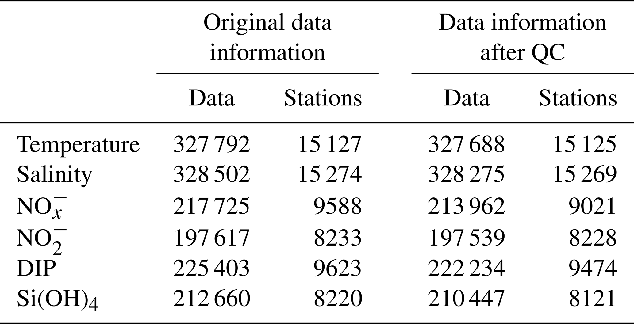
Field observations were originally downloaded from the Climate and Ocean: Variability, Predictability, and Change (CLIVAR) and Carbon Hydrographic Data Office (CCHDO), which distributes vessel-based hydrographic data from programs such as the World Ocean Circulation Experiment (WOCE), Joint Global Ocean Flux Study (JGOFS), GO-SHIP, CLIVAR, and other repeat hydrography efforts (https://cchdo.ucsd.edu/, last access: 1 October 2024). In total, 631 cruises were collected in the North Pacific, comprising 228 091, 197 617, 225 403, and 212 660 data points for NO${}_{\mathrm{3}}^{-}$ + NO${}_{\mathrm{2}}^{-}$ (NO${}_x^{-}$), NO${}_{\mathrm{2}}^{-}$, DIP, and Si(OH)₄, respectively (Table 1). The dataset spans from 1973 to 2022 and was downloaded on 1 October 2024; any updates made after this date were not included in this study. The data cover a geographic range from 120.08° E to 95.17° W and from 2.05° S to 60.25° N. The study domain was slightly extended into the South Pacific to mitigate potential boundary effects during model development.

Table 1 Information on nutrients and their associated hydrographic data collected from CLIVAR and Carbon Hydrographic Data Office (CCHDO) and the information after quality control (QC).

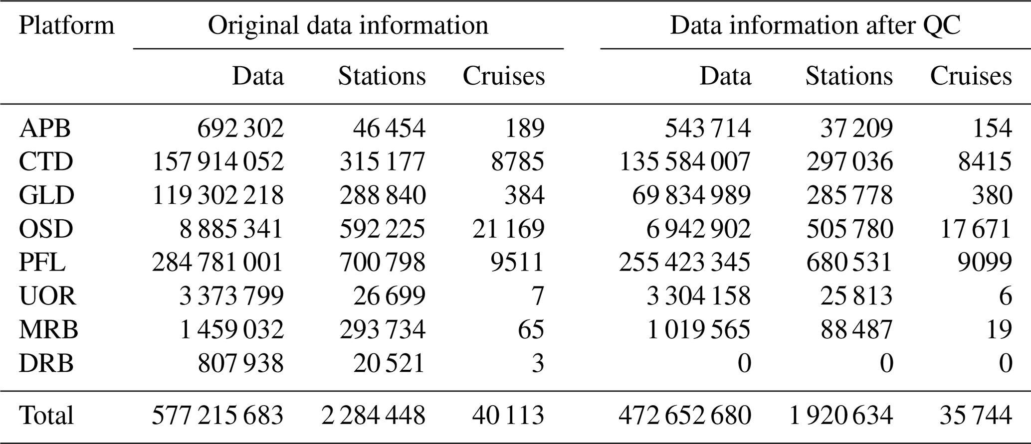
Hydrographic data for nutrient reconstruction were obtained from the World Ocean Database (WOD; Mishonov et al., 2024), which compiles observations from various platforms, including Autonomous Pinniped Bathythermograph (APB), Conductivity-Temperature-Depth profiler (CTD), Drifting Buoy (DRB), Glider (GLD), Mechanical Bathythermograph (MBT), Moored Buoy (MRB), Ocean Station Data (OSD), Profiling Float (PFL), and Undulating Oceanographic Recorder (UOR). Since nutrient reconstruction models rely on relationships with water masses, only samples containing both temperature and salinity measurements were used; therefore, most APB observations, which record only temperature, were excluded. Among these platforms, CTD, OSD, and PFL provided the majority of usable data. Additionally, several marginal seas – including the South China Sea, the Yellow Sea, the Sea of Japan, and the Sea of Okhotsk – were excluded from this study because they are semi-enclosed and strongly influenced by terrestrial inputs. The spatial domain was consistent with that used for the CCHDO dataset, while the temporal coverage extended from 1875 to 2024. In total, 577 215 683 data points from 2 284 448 stations across 40 113 original cruises were collected (Table 2). In addition, the OSD data before 1970 were extracted for nutrient validation in Sect. 3.1. A total of 102 424, 125 142, 447 335, and 294 734 data points were collected for NO${}_{\mathrm{3}}^{-}$, NO${}_{\mathrm{2}}^{-}$, DIP, and Si(OH)₄, respectively.

Table 2 Information on hydrographic data collected from World Ocean Database, and the data information after quality control (QC). See main text for acronyms' full names.

2.2 Data quality control

Given that the data were collected from multiple platforms using various methods over a long-time span and broad spatial range, quality control (QC) was essential (Du et al., 2021; Wang et al., 2025). Following the QC procedures developed by the World Ocean Database (WOD) (Garcia et al., 2024), we applied comprehensive QC protocols (Fig. 1) to both CCHDO and WOD datasets, including hydrographic and nutrient variables.

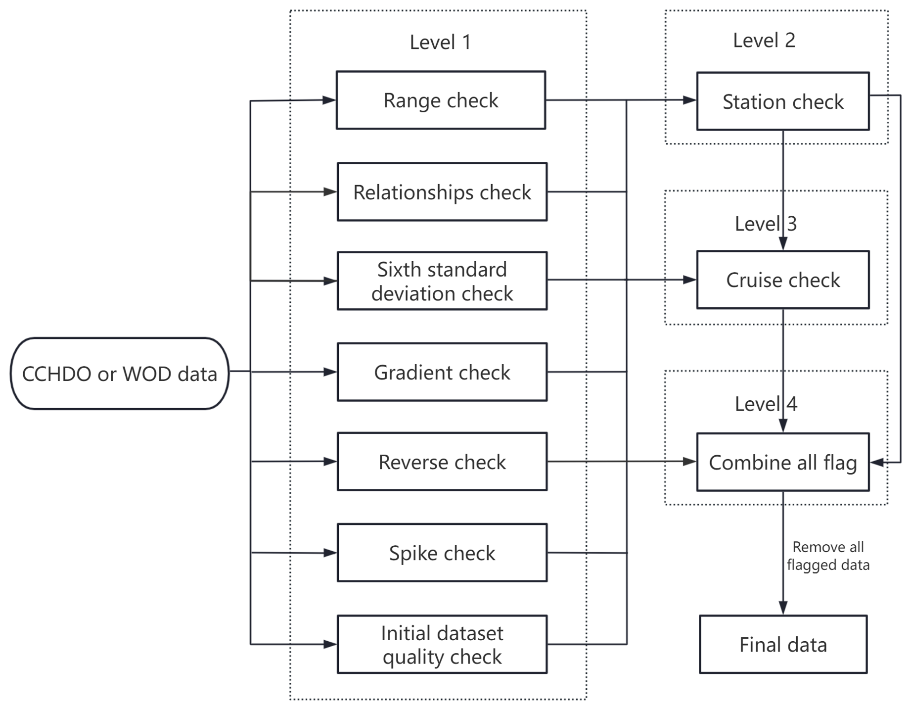
Figure 1 Data quality control procedures for temperature, salinity and nutrients collected from the CLIVAR and Carbon Hydrographic Data Office (CCHDO) and the World Ocean Database (WOD) datasets.

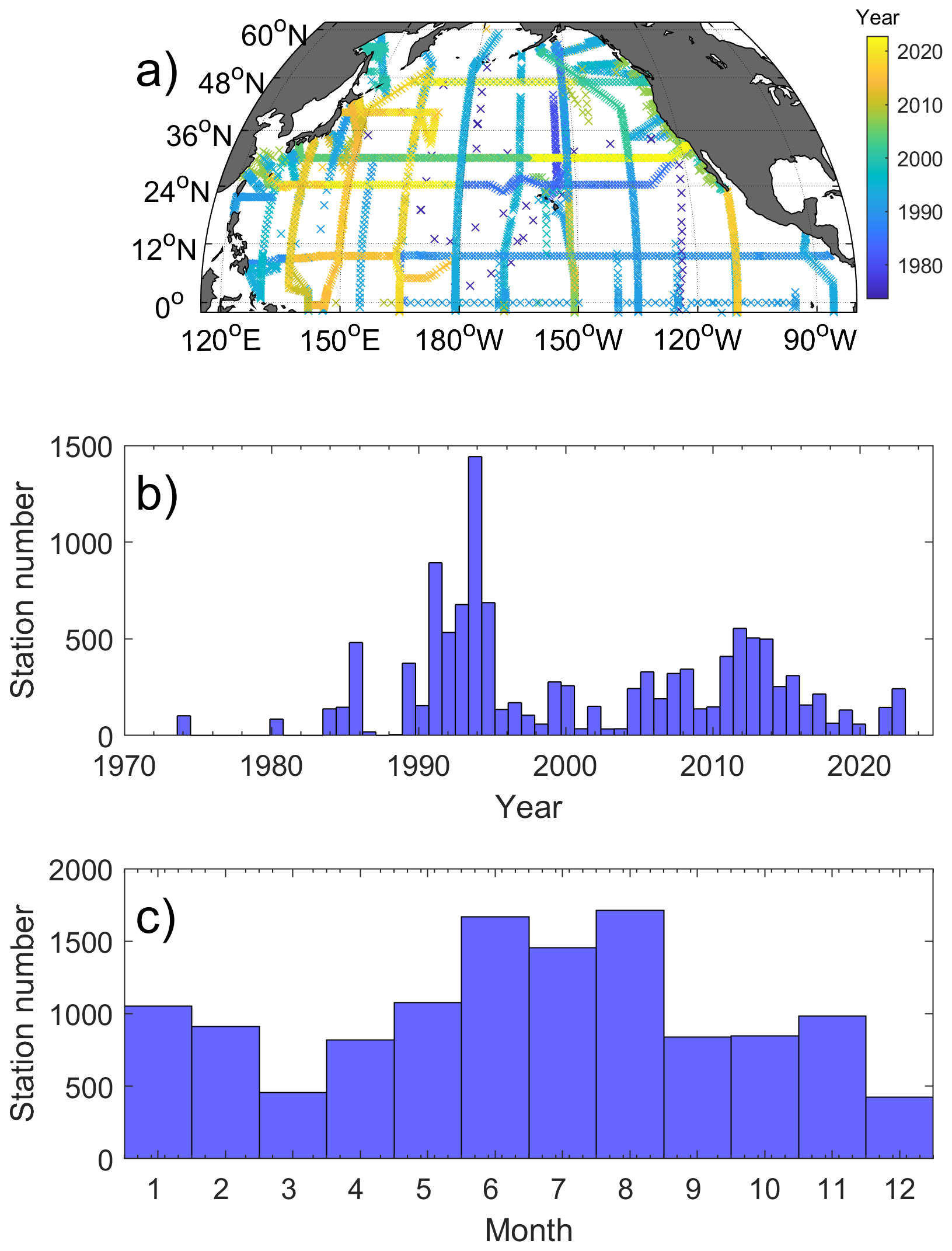
Figure 2 Spatial and temporal distributions of NO${}_x^{-}$ (nitrate plus nitrite) after quality control in the North Pacific. (a) Distribution of NO${}_x^{-}$ data locations, with points color-coded by year; (b) station counts per year; (c) station counts per month.

Four levels of QC were applied to identify and remove potentially erroneous or low-quality records from the CCHDO and WOD datasets. The first level targeted individual measurements, including several checks. (1) A range check was conducted by defining depth-dependent acceptable value ranges for each parameter; data falling outside these ranges were flagged as invalid. This check was applied to temperature, salinity, NO${}_x^{-}$, NO${}_{\mathrm{2}}^{-}$, DIP, and Si(OH)₄. Note that the NO${}_x^{-}$ denotes the sum concentration of NO${}_{\mathrm{2}}^{-}$ and NO${}_{\mathrm{3}}^{-}$. At stations lacking direct NO${}_x^{-}$ measurements, NO${}_x^{-}$ concentrations were derived by summing discrete NO${}_{\mathrm{2}}^{-}$ and NO${}_{\mathrm{3}}^{-}$ observations. (2) An empirical relationship check was performed to verify consistency among paired variables based on predefined acceptable domains, including temperature–salinity, temperature–NO${}_x^{-}$, temperature–NO${}_{\mathrm{2}}^{-}$, temperature–DIP, temperature–Si(OH)₄, salinity–NO${}_x^{-}$, salinity–NO${}_{\mathrm{2}}^{-}$, salinity–DIP, salinity–Si(OH)₄, NO${}_x^{-}$–DIP, and NO${}_x^{-}$–Si(OH)₄. (3) A six-standard-deviation check was conducted by calculating the mean and standard deviation at each depth level; values falling beyond six standard deviations were flagged as outliers. (4) A gradient check assessed the vertical gradients of each parameter at each depth level across stations; data showing abnormal gradients exceeding five standard deviations from the mean were flagged as questionable. (5) A depth/potential density (σ_θ) inversion check was applied to detect unrealistic reversals in parameters such as temperature and nutrients, which typically exhibit monotonic relationships with depth or σ_θ in stratified waters; measurements violating preset thresholds for depth–temperature, depth–NO${}_x^{-}$, depth–DIP, depth–Si(OH)₄, σ_θ–temperature, σ_θ–NO${}_x^{-}$, σ_θ–DIP, and σ_θ–Si(OH)₄ were flagged. (6) A spike check was implemented to identify abrupt deviations (spikes) between a measurement and its adjacent vertical neighbors; if the difference exceeded a defined threshold, the data point was flagged as suspect. This check was applied to temperature, NO${}_x^{-}$, DIP, and Si(OH)₄. (7) Only measurements with an original quality flag of “good” from CCHDO and WOD were retained, while those marked as questionable or erroneous were flagged as outliers.

Building on the individual-level QC, we implemented additional QC at the station and cruise levels. At the station level, if a station profile contained more than 20 % flagged data points, all data from that station were flagged as questionable. At the cruise level, if over 30 % of a cruise's data were flagged, all data from that cruise were flagged. The final step integrated flags from all three levels (individual, station, and cruise), and any data flagged at any level were excluded. This hierarchical QC protocol effectively eliminates low-quality data. Although this approach may discard some high-quality measurements, the large volume of available data necessitates strict QC to ensure reliability.

After quality control, the CCHDO dataset retained 214 943 (9120), 197 539 (8228), 222 234 (9457) and 210 447 (8123) data points (stations), accounting for 94.2 % (95.1 %), 100.0 % (99.9 %), 98.6 % (98.5 %) and 99.0 % (98.8 %) of the original data points (stations) for NO${}_x^{-}$, NO${}_{\mathrm{2}}^{-}$, DIP, and Si(OH)₄, respectively (Table 1). The retained stations cover nearly the entire North Pacific Ocean (Fig. 2a), spanning from 1972 to 2023. Most observations were collected after 1980, with a substantial increase after 1990 (Fig. 2b). Seasonally, the number of stations in June, July, and August was approximately three times greater than that in March and December (Fig. 2c).

Following quality control, the final WOD dataset comprised 472 652 680 temperature and salinity data points from 1 920 634 stations across 35 744 cruises, spanning 1895 to 2024. These represent 81.9 % of the original observations, 84.1 % of the original stations, and 89.1 % of the original cruises, respectively (Table 2). Spatially, station counts per 1°×1° grid cell range from 1 to 31 851, with a mean of 249 stations per cell (Fig. 3a). High sampling densities are found off eastern Japan and western North America, resulting from high frequency observations from CTD and OSD platforms, whereas elevated counts in the southwestern North Pacific primarily result from MRB observations. Temporally, fewer than 300 stations per year were collected before 1930. The annual number of stations exceeded 10 000 after 1964 and peaked at approximately 100 000 in 2021 (Fig. 3b). Seasonally, station numbers are highest from May to August (Fig. 3c). Overall, the collected WOD dataset provides 2127–2393 times more observations and 202 times more station records than the CCHDO dataset.

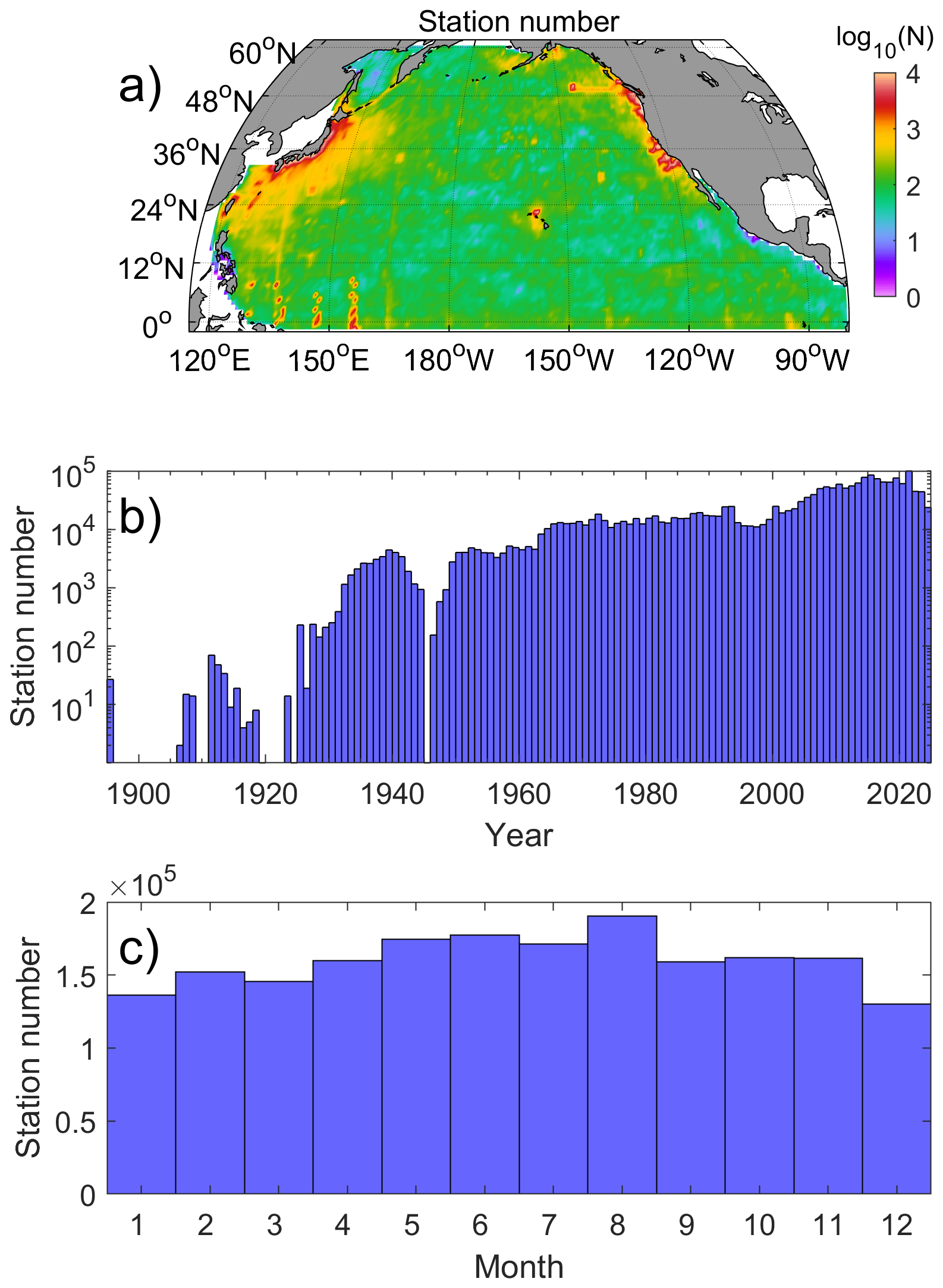
Figure 3 Spatial and temporal distribution of the World Ocean Database (WOD) data after quality control. (a) Station counts per 1°×1° grid cell; (b) station counts per year; (c) station counts per month.

2.3 Machine learning and nutrient reconstruction

After rigorous data quality control, CCHDO data were used to train machine learning models. Three algorithms including Random Forest (RF), Light Gradient Boosting Machine (LightGBM), and Gaussian Process Regression (GPR) were applied to establish the relationship between environmental parameters and nutrient concentrations (Fig. 4). These methods are widely used in marine science (Hu et al., 2021; Huang et al., 2022; Yu et al., 2024; Chen et al., 2023; Sundararaman and Shanmugam, 2024). The use of diverse models helps reduce algorithm selection bias. RF is an ensemble technique based on bagging, which builds multiple independent decision trees and aggregates their outputs by voting or averaging (Liaw and Wiener, 2002). Its strengths include high predictive accuracy and reduced overfitting owing to the large number of trees. RF has been applied to predict global primary production (Huang et al., 2021), chlorophyll concentrations (Madani et al., 2024), nutrients (Chen et al., 2023, 2024), dissolved iron (Huang et al., 2022), surface ocean pCO₂ (Chen et al., 2019), and N₂ fixation rates (Yu et al., 2024).

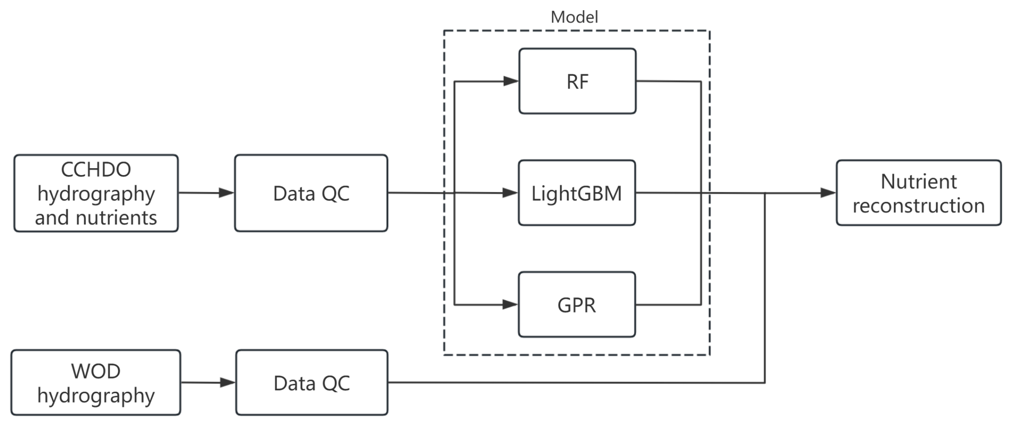
Figure 4 Flowchart of the machine learning framework and its application to WOD hydrographic data for nutrient reconstruction.

LightGBM is an ensemble learning algorithm based on Gradient Boosting Decision Trees (GBDT). Compared to standard GBDT, LightGBM employs a leaf-wise tree growth strategy and a histogram-based binning technique to improve predictive accuracy and computational efficiency (Ke et al., 2017). It has been successfully applied to predict water levels (Gan et al., 2021), salinity (Dong et al., 2022; Wang et al., 2022), and chlorophyll a concentration (Su et al., 2021). GPR is a non-parametric Bayesian approach that infers relationships by defining a prior distribution over functions via kernel-based covariance matrices, rather than estimating fixed coefficients. This flexibility allows GPR to capture complex, nonlinear input–output relationships and to quantify prediction uncertainty. GPR has been used in oceanography to estimate global dissolved oxygen and nutrient concentrations (Sundararaman and Shanmugam, 2024).

In this study, we used spatial coordinates (longitude, latitude, depth), temporal variables (month and year), and water mass properties (represented by potential temperature and salinity) as environmental predictors of nutrient concentrations. The time predictors used month and year with decimals to capture seasonal, interannual, and long-term variability. The North Pacific contains distinct water masses, including North Pacific Subtropical Water, North Pacific Intermediate Water, Antarctic Intermediate Water, Western South Pacific Central Water, North Pacific Deep Water, and Pacific Deep Water, as well as Circumpolar Deep Water (e.g., Talley et al., 2011; Fuhr et al., 2021). These water masses mix to form different water types associated with distinct nutrient concentrations (Fig. 5). Water types have been found to be an important parameter to reconstruct nutrient concentrations in the South China Sea (Du et al., 2021). Thus, potential temperature and salinity serve as proxies for water mass identification.

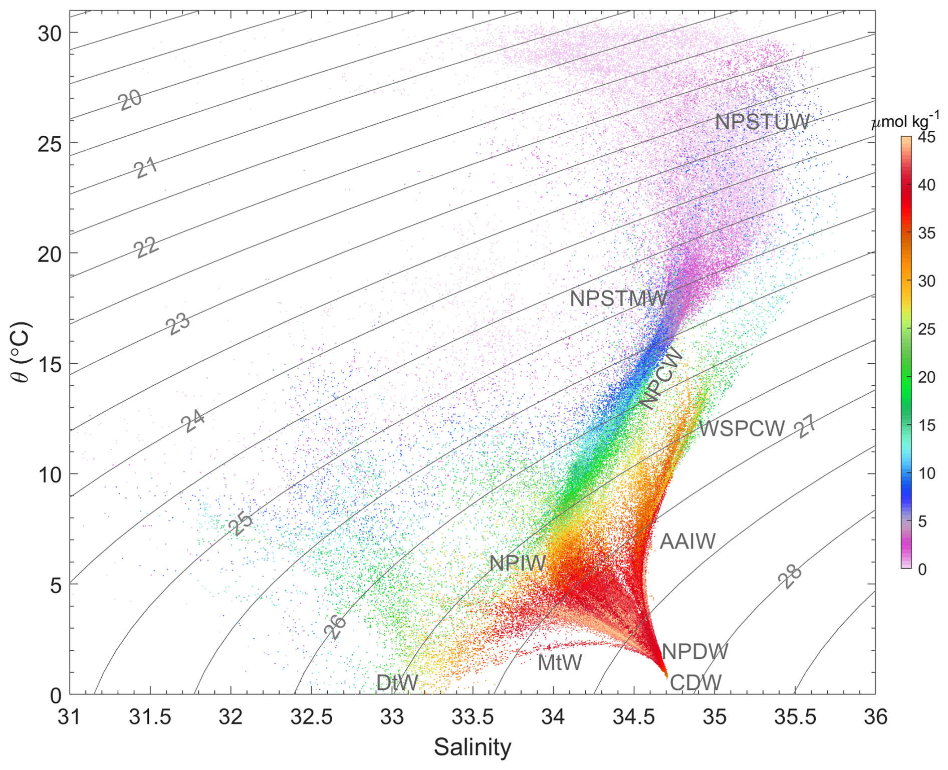
Figure 5 The water masses – indicated by salinity and potential temperature (θ) – and NO${}_x^{-}$ (NO${}_{\mathrm{3}}^{-}$ + NO${}_{\mathrm{2}}^{-}$; color shading) relationships in the North Pacific. The temperature and salinity data were collected from the CCHDO dataset. The gray contour lines and number denote the potential density anomaly. The typical water masses are shown as follows: North Pacific Central Water (NPCW), North Pacific Subtropical Underwater (NPSTUW), North Pacific Subtropical Mode Water (NPSTMW), North Pacific Intermediate Water (NPIW), Dichothermal Water (DtW), Mesothermal Water (MtW), Antarctic Intermediate Water (AAIW), Western South Pacific Central Water (WSPCW), Pacific Deep Water (PDW), and Circumpolar Deep Water (CDW). The water masses and their acronyms are following the classifications in Talley et al. (2011) and Fuhr et al. (2021).

3 Results

3.1 Error estimation

Leave-one-out cross-validation was primarily used to quantify model reconstruction errors. The CCHDO dataset was divided into training and testing subsets for model development and performance evaluation, respectively. To assess how data partitioning affects error metrics, we implemented four validation methods based on different data-selection strategies (Fig. 6a). The first three methods involved partitioning the CCHDO dataset into training (80 %) and testing (20 %) subsets. These methods employed three data selection strategies: (1) sample-random, by withholding 20 % of individual samples; (2) station-random, by withholding 20 % of stations; and (3) cruise-random, by withholding 20 % of cruises. Predictions for the held-out subsets, generated using their respective spatial, temporal, and water mass property data, were compared against the actual withheld nutrient measurements to calculate error metrics. These partitioning strategies were designed to evaluate potential errors under the sparse and non-uniform spatiotemporal distribution of observations: Error 1 represented an optimistic estimate (validation data are likely co-located with training data in space and time), Error 3 represented a conservative, generalized scenario (validation data are independent of training data), Error 2 provided an intermediate estimate (validation data may share spatial/temporal context with training data within the same cruise). The choice of error metric (Error 1, 2, or 3) should be guided by the degree of extrapolation in the intended application relative to the training data's spatiotemporal distribution.

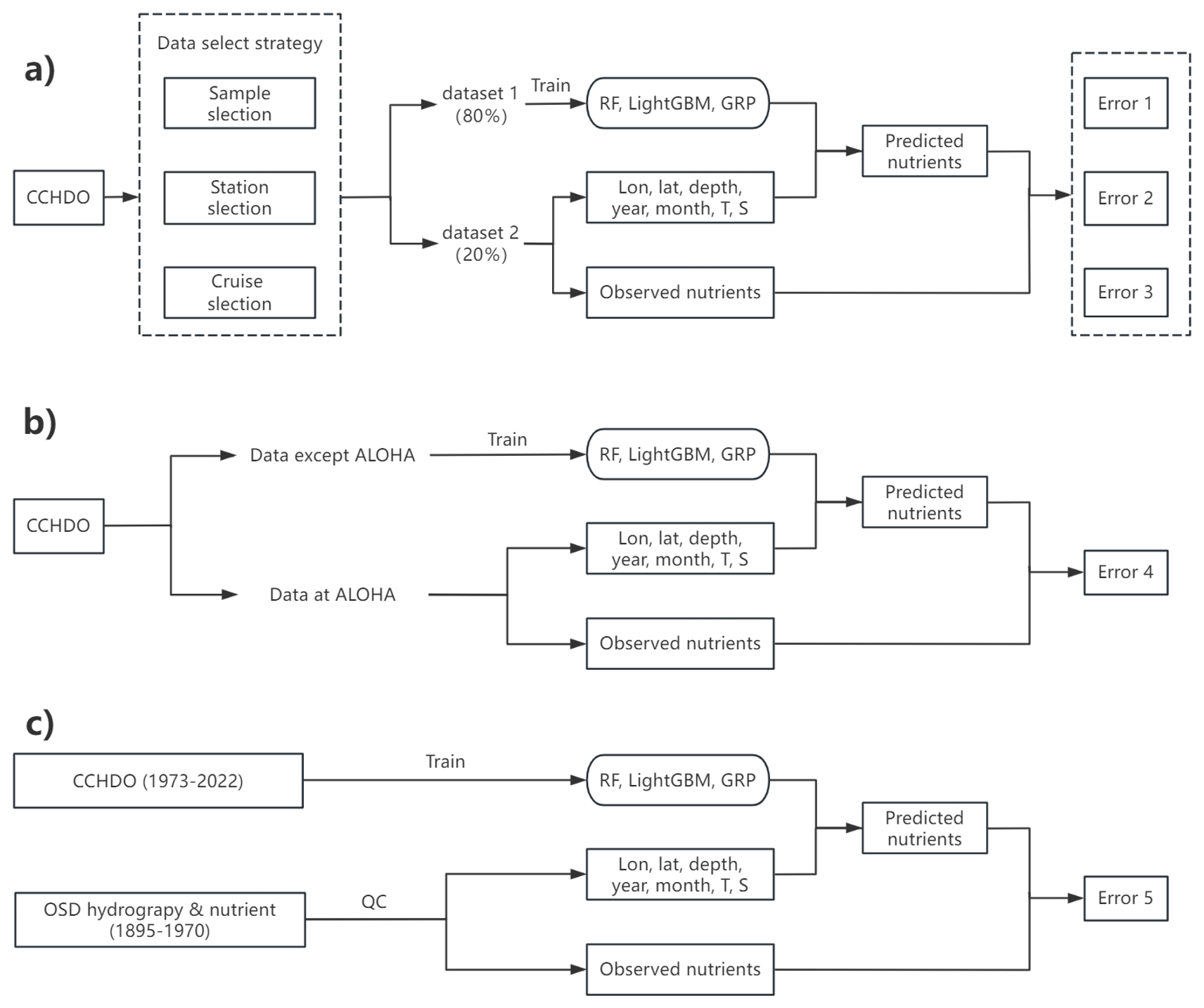
Figure 6 Schematic of the error estimation procedure. (a) Error estimation based on three types of data selection strategy; (b) assessing temporal error evolution by excluding the data at Station ALOHA; (c) examining the models' reconstruction error using the hydrographic and nutrient data before 1970. The T and S denote the potential temperature and salinity, respectively.

The validation results for reconstructed NO${}_x^{-}$ versus observations under the first three data-selection strategies are shown in Fig. 7. RF and GPR exhibited nearly identical performance, with regression slopes of 0.992–0.998, R²>0.992, and Root Mean Squared Errors (RMSEs) between 0.734 and 1.313 µmol kg⁻¹ (Fig. 7a, c, d, f, g and i). LightGBM showed slightly lower accuracy (slope: 0.991–0.995; R²: 0.991–0.996; RMSEs: 0.780–1.419 µmol kg⁻¹) (Fig. 7b, e and h). Across different data-selection strategies, sample-random (Error 1) yielded the lowest errors (RMSEs: 0.734–0.983 µmol kg⁻¹) (Fig. 7a–c), station-random (Error 2) was intermediate (RMSEs: 0.908–1.313 µmol kg⁻¹) (Fig. 7d–f), and cruise-random (Error 3) produced the highest errors (RMSEs: 1.243–1.424 µmol kg⁻¹) (Fig. 7; Table 3). This gradient in error estimates underscores the necessity of employing different data-selection strategies for a comprehensive error assessment. The high slopes and R² values (>0.99) achieved across all algorithms and data-selection strategies confirmed the robustness of the nutrient reconstructions.

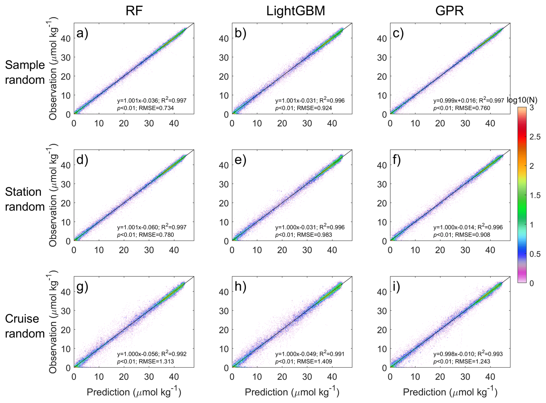
Figure 7 Validating the reconstructed NO${}_x^{-}$ concentrations using leave-one-out cross-validation with different data selection strategies and machine learning methods. Plots shown in row 1 correspond to the sample random strategy (a–c), row 2 correspond to the station random strategy (d, e), and row 3 correspond to the cruise random strategy (g–i). Plots shown in column 1 correspond to the Random Forest (RF; a, d, g), column 2 correspond to the LightGBM (b, e, h), and column 3 correspond to the Gaussian Process Regression (GPR; c, f, i). The black lines and text show the fitted linear regressions, regression equations, coefficient of determination (R²), p values, and Root Mean Squared Errors (RMSEs). The color represents the data density (N, number of observations). Note that a logarithmic scale is applied to N.

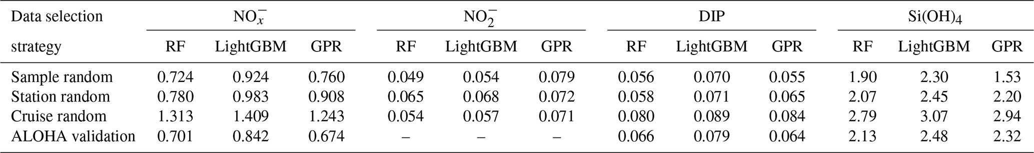
Table 3 The Root Mean Squared Errors of nutrient reconstruction from different error evaluation strategies (unit: µmol kg⁻¹).

Reconstruction errors for NO${}_{\mathrm{2}}^{-}$, DIP, and Si(OH)₄ are summarized in Figs. S1–S3 in the Supplement and Table 3. Across methods, the RMSEs were below 0.079 µmol kg⁻¹ for NO${}_{\mathrm{2}}^{-}$, 0.089 µmol kg⁻¹ for DIP, and 3.07 µmol kg⁻¹ for Si(OH)₄. DIP and Si(OH)₄ exhibited similar error trends: RMSEs increased from sample-random to station-random to cruise-random selection. In contrast, NO${}_{\mathrm{2}}^{-}$ reconstruction exhibited lower accuracy than NO${}_x^{-}$, DIP, and Si(OH)₄, with regression slopes of 0.48–0.68 and R² values of 0.32–0.72. RF and LightGBM outperformed GPR for NO${}_{\mathrm{2}}^{-}$. The poorer NO${}_{\mathrm{2}}^{-}$ performance likely reflects its generally low concentrations (mostly <0.5 µmol kg⁻¹) and high biological variability. Thus, we highlight NO${}_{\mathrm{2}}^{-}$ as a high-uncertainty reconstruction.

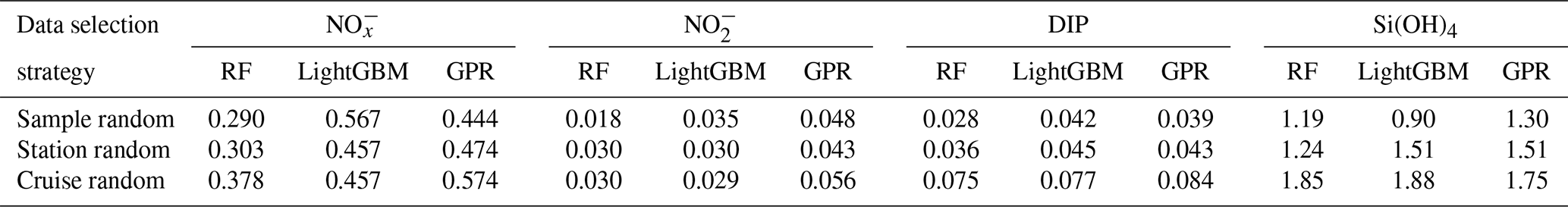
Understanding the spatiotemporal structure of reconstruction errors is also important for assessing the models' reconstruction applicability. As shown in Figs. S4–S7, the reconstruction errors of NO${}_{\mathrm{3}}^{-}$, DIP, and Si(OH)₄ are generally small in the surface layer, increase with depth to maxima at the nutricline, and then decrease to low values in deep layers. However, the random errors associated with individual cruise observations for Si(OH)₄ display no evident vertical pattern. Horizontally, we paid particular attention to surface waters due to their greatest concentration gradients. The horizontal distribution shows that the errors are small in the western NPSG (a nutrient-depleted region) but are large in the subarctic gyre and close to the equatorial regions (nutrient-replete regions; Figs. S8–S11). Here, we particularly examined the nutrient reconstruction errors in the oligotrophic NPSG. The oligotrophic regimes are defined as regions where NO${}_{\mathrm{3}}^{-}$, NO${}_{\mathrm{2}}^{-}$, DIP, and Si(OH)₄ concentrations are <0.2, <0.2, <0.2, and <5.0 µmol kg⁻¹, respectively. As shown in Table 4, the reconstruction errors in these regimes are <0.574, <0.056, <0.084, and <1.88 µmol kg⁻¹ for NO${}_{\mathrm{3}}^{-}$, NO${}_{\mathrm{2}}^{-}$, DIP, and Si(OH)₄, respectively, which are evidently lower than the overall RMSEs for the entire North Pacific (Table 3). Among these models, the RF generally performs the best compared to the others. This confirms that absolute errors decrease in oligotrophic regimes. Since the number of summer observations is up to three times greater than that in winter and spring, we further examined the seasonal variation of errors. Overall, no evident seasonal variations are displayed. Only in the case of random cruise selection was the NO${}_{\mathrm{3}}^{-}$ error shown to be greater in spring (March to May) than in other seasons (Fig. S12). For other cases and nutrients, seasonal variation in error was not evident. On a decadal timescale, the reconstruction errors display a slight decreasing trend, particularly for DIP, from 1973 to 2020 (Fig. S13), implying that the errors might be smaller in recent decades than in previous ones.

Table 4 The Root Mean Squared Errors of nutrient reconstruction from different error evaluation strategies in surface oligotrophic regimes (unit: µmol kg⁻¹).

A fourth validation step assessed the model's temporal performance at Station ALOHA (Error 4; Fig. 6b). To test this, we withheld all observations from ALOHA (which, since 1988, represent 8.52 %, 8.45 %, and 8.11 % of the total Si(OH)₄, NO${}_x^{-}$, and DIP records, respectively) from model training. We then reconstructed nutrient concentrations using space, time, and water-type predictors at Station ALOHA. NO${}_{\mathrm{2}}^{-}$ was excluded due to insufficient observations. For NO${}_x^{-}$, the regression slopes between reconstruction and observations were 0.99, 0.98, and 0.99, with RMSEs of 0.701, 0.842, and 0.674 µmol kg⁻¹ for RF, LightGBM, and GPR, respectively; R² values exceeded 0.997 for all models (Fig. 8a). RF and GPR slightly outperformed LightGBM. All models accurately reproduced the NO${}_x^{-}$ profiles (Fig. 8b). The reconstruction errors for DIP were 0.066, 0.079, and 0.064 µmol kg⁻¹ for RF, LightGBM, and GPR, respectively. The corresponding errors for Si(OH)₄ were 2.13, 2.48, and 2.32 µmol kg⁻¹ (Table 3, Figs. S14 and S15).

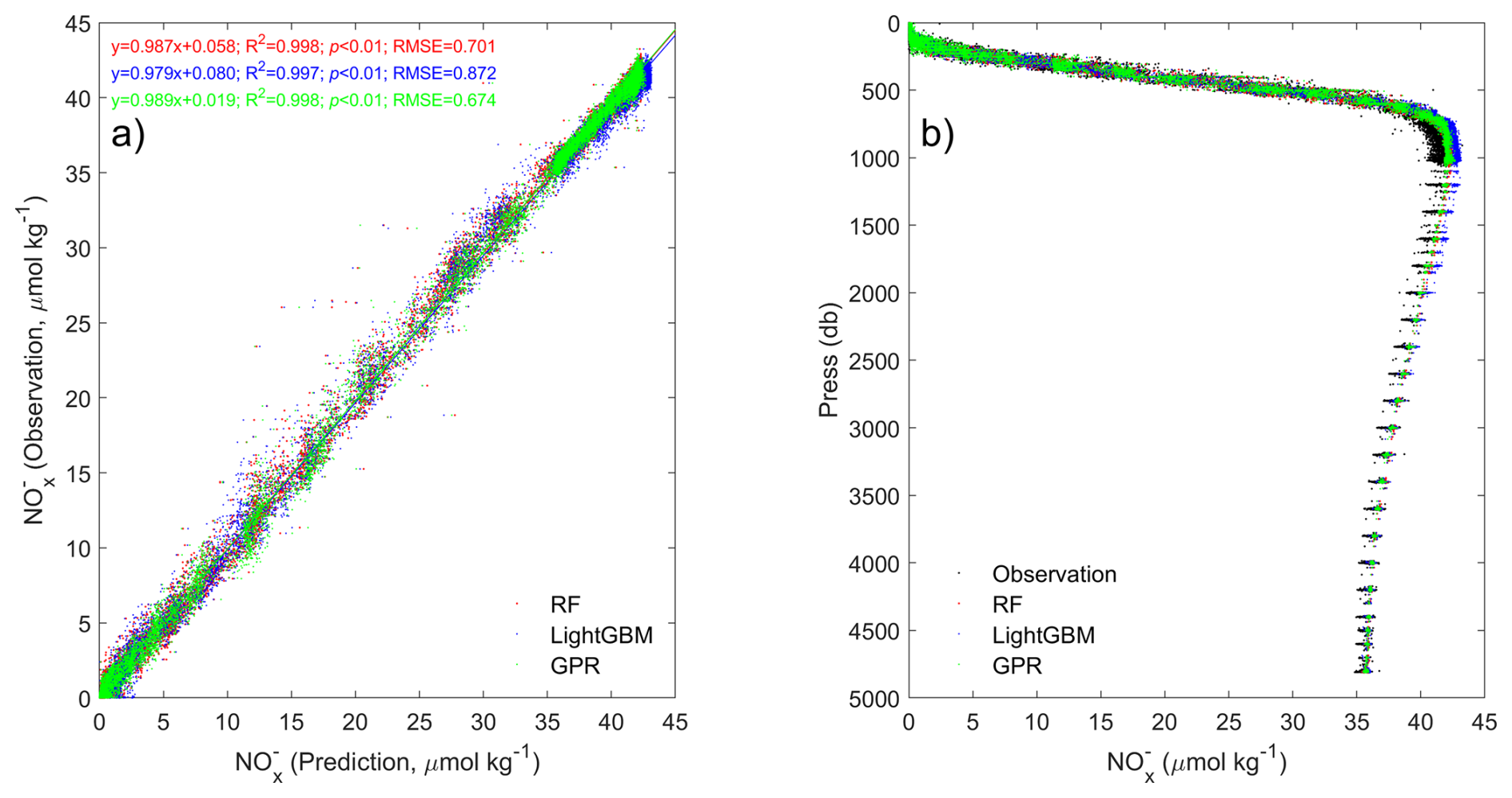
Figure 8 Validating the reconstructed nutrient concentrations at Station ALOHA. (a) Reconstructed NO${}_{\mathrm{3}}^{-}$ + NO${}_{\mathrm{2}}^{-}$ (NO${}_x^{-}$) vs. observations: Random Forest (RF; red dots), LightGBM (blue dots), and Gaussian Process Regression (GPR; green dots). (b) Profiles of observed (black dots) and reconstructed NO${}_x^{-}$ from RF (red dots), LightGBM (blue dots), and GPR (green dots).

Since the variations of nutrients primarily occur in the upper water column, we focused on the nutrient reconstruction in the upper 300 m at Station ALOHA. Overall, the models reproduced the profiles of NO${}_x^{-}$ from 1988 to 2021 well (Fig. 9a–d). The reconstruction errors were low at the surface and increased with depth, with most of the values < 3.0 µmol kg⁻¹ (Fig. S16a–d). To evaluate models' ability to reconstruct nutrient variations in time, the nutrient concentrations were averaged monthly over the upper 300 m. As compared to observations, RF, LightGBM, and GPR all well reconstructed the interannual variations of NO${}_x^{-}$ with most of the absolute errors < 0.5 µmol kg⁻¹ (Figs. 9e and S16e) at Station ALOHA. Similarly, the validation of DIP and Si(OH)₄ are shown in Figs. S17–S20.

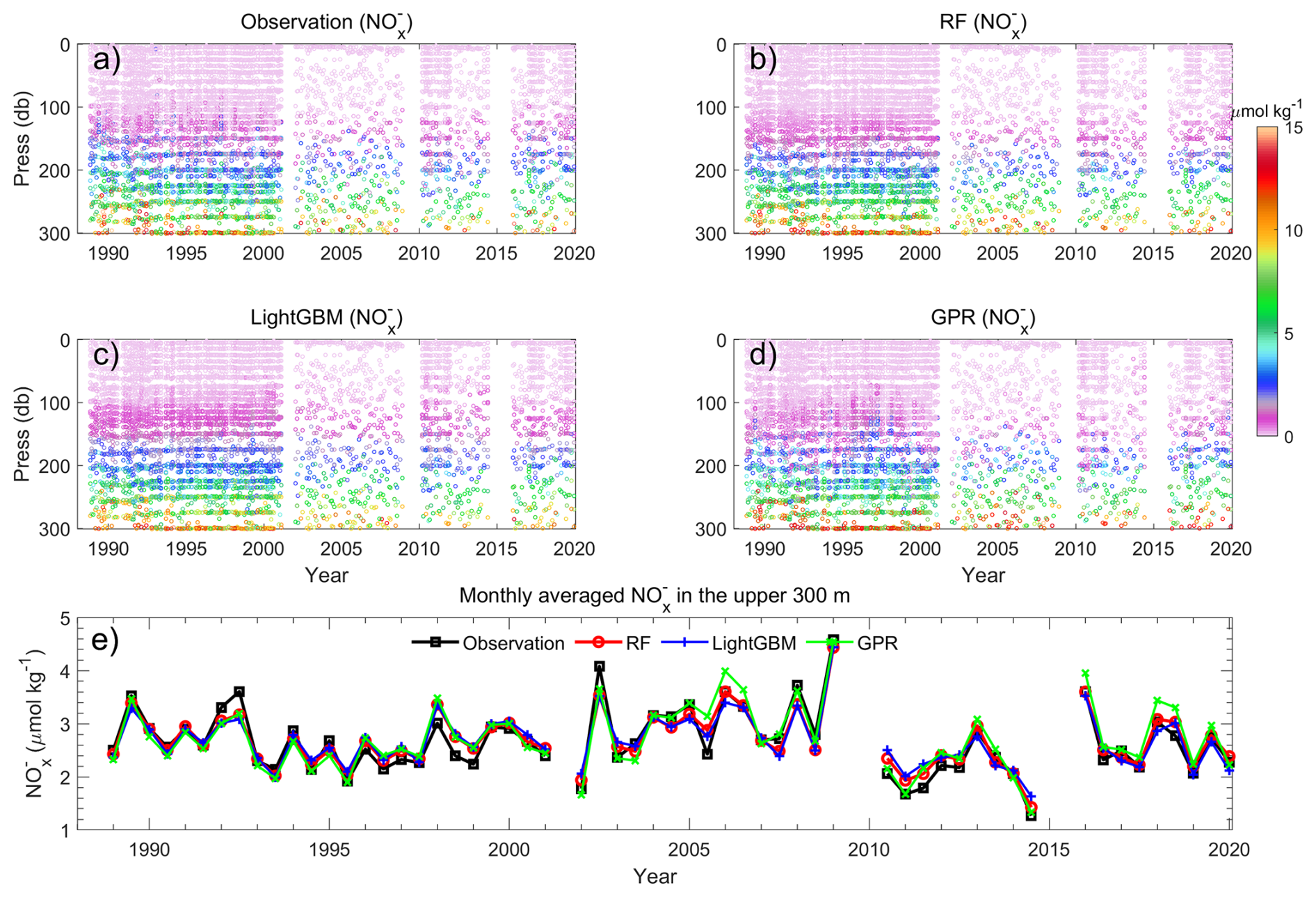
Figure 9 Temporal variations of NO${}_x^{-}$ concentrations in the upper 300 m at Station ALOHA from 1988 to 2021 for observed (a) and reconstructed NO${}_x^{-}$ by Random Forest (RF; b), LightGBM (c), and Gaussian Process Regression (GPR; d). (e) Time series of monthly averaged NO${}_x^{-}$ concentrations in the upper 300 m from observations, and reconstructions by RF, LightGBM, and GPR.

A fifth validation step evaluates the models' reconstruction for the period before 1970 (Error 5; Fig. 6c). This is necessary because the training data (CCHDO) spans 1973–2022, while the reconstructions are extrapolated back to 1895. We argue that this extrapolation should be reasonable because the variations of temperature–salinity–nutrient relationships in the ocean's interior might be small over the past century, providing a basis for temporal extrapolation. First, the residence time of nitrogen in deep and intermediate waters can be up to 2000 years in the North Pacific. Consequently, the imprint of centennial-scale change on nutrient inventories is attenuated. Second, the long-term variations of nutrient concentrations are not evident within our core training period (1973–2022; Figs. 9e and 17). Finally, the mean nutrient profiles derived from the 1920–1970 and 1973–2022 periods are not evidently different in the central North Pacific (Fig. S21). Therefore, while the North Pacific may experience long-term variability, it might be masked by the reconstruction error, and the use of hydrographic properties as predictors for nutrients is justified for historical reconstructions.

However, when assessing the reconstruction errors before 1970, we first consider data quality issues. Prior to the standardization of modern oceanographic methods, nutrient measurements – particularly from earlier decades – were subject to greater analytical errors, inconsistent sampling protocols, and varied determination techniques. The data quality concern is evident in the sporadic and sometimes physically implausible deep nutrient profiles found in WOD for that era (Fig. S22). This is also the primary reason that nutrient data pre-1973 collected from sources like the OSD from WOD were not incorporated into model training. To evaluate data quality in earlier decades, we selected five specific years with more abundant observations: 1929, 1947, 1953, 1958, and 1966 (Fig. S23). After applying the same quality-control criteria outlined in Sect. 3.1, we used the historical hydrographic data (temperature and salinity) from those years to predict nutrient concentrations. A total of 52 277, 119 137, 284 472, and 193 339 data points were collected for NO${}_{\mathrm{3}}^{-}$, NO${}_{\mathrm{2}}^{-}$, DIP, and Si(OH)₄, respectively, after QC. The comparison between these predictions and the quality-controlled observations yields the prediction errors for the pre-1970 period (Fig. 6c). The RMSEs from different models suggested values <5.7, <0.40, and <22.9 µmol kg⁻¹ for NO${}_{\mathrm{3}}^{-}$, DIP, and Si(OH)₄, respectively (Figs. S24–S26), which are much larger than the corresponding errors for the period after 1970. We recommend that these values be considered a conservative estimate of the upper error bound, as they incorporate both nutrient observations and prediction errors. In addition, the hydrographic data are also less reliable in the earlier period. Thus, we acknowledge that reconstruction errors are likely higher for the pre-1973 period, and the error estimated here should be considered a “best estimate” with quantified uncertainties, and encourage users to consider these error bounds when applying the dataset to early 20th century conditions.

3.2 Reconstructed nutrients

The final reconstructed nutrient dataset aligns with the spatiotemporal coverage of the quality-controlled WOD hydrographic dataset, comprising 472 652 680 data points for each nutrient (NO${}_x^{-}$, NO${}_{\mathrm{2}}^{-}$, DIP, and Si(OH)₄) from 1 920 634 stations across 35 744 cruises, spanning from 1895 to 2024 (Table 2). Most data points are located above 2000 m, with fewer observations at greater depths due to hydrographic platform limitations.

It is important to clarify the nature of the reconstructed dataset, which is fundamentally different from gridded products. This product provides nutrient concentrations linked to each hydrographic observations: nutrient values are reconstructed precisely at the locations, depths, and times of original hydrographic observations (sourced from WOD) where direct nutrient measurements might be unavailable or of poor quality. This approach yields a point-wise dataset that aligns with the original hydrographic observations, rather than a spatially or temporally interpolated field – an important distinction for users interpreting and applying the data.

3.3 Climatology of nutrient distributions

To evaluate the reliability of our product, we binned and averaged the predicted nutrients within 1°×1° grid cells for each month to produce a monthly climatology. This climatology represents a mean field that depends heavily on the spatiotemporal distribution of the underlying data and may be influenced by uneven data sampling. This reconstructed climatology was compared with the World Ocean Atlas 2023 (WOA23), which is derived from quality-controlled and objectively analyzed observational data. Since the large-scale patterns of NO${}_{\mathrm{3}}^{-}$, DIP, and Si(OH)₄ are similar among different models (Figs. 10–13 and S27–S36), we focus on NO${}_{\mathrm{3}}^{-}$ reconstructed by the RF model in this section unless stated otherwise.

Figures 10–13 present the monthly climatology of NO${}_x^{-}$ at 5, 100, 500, and 1000 m in the North Pacific. At 5 m, the reconstructed NO${}_x^{-}$ accurately captures the established spatial patterns, with elevated concentrations in the subpolar gyre, Bering Sea, and equatorial regions, and depleted concentrations in the NPSG (Fig. 10). Seasonally, the basin-averaged surface NO${}_x^{-}$ concentrations display the highest value of 3.50 µmol kg⁻¹ in March, in contrast to the lowest value of 1.82 µmol kg⁻¹ in September. These results agree with Yasunaka et al. (2014, 2021), who, using extensive surface nutrient observations (up to 14 000 for nitrate) in the North Pacific, reported similar spatial and seasonal patterns.

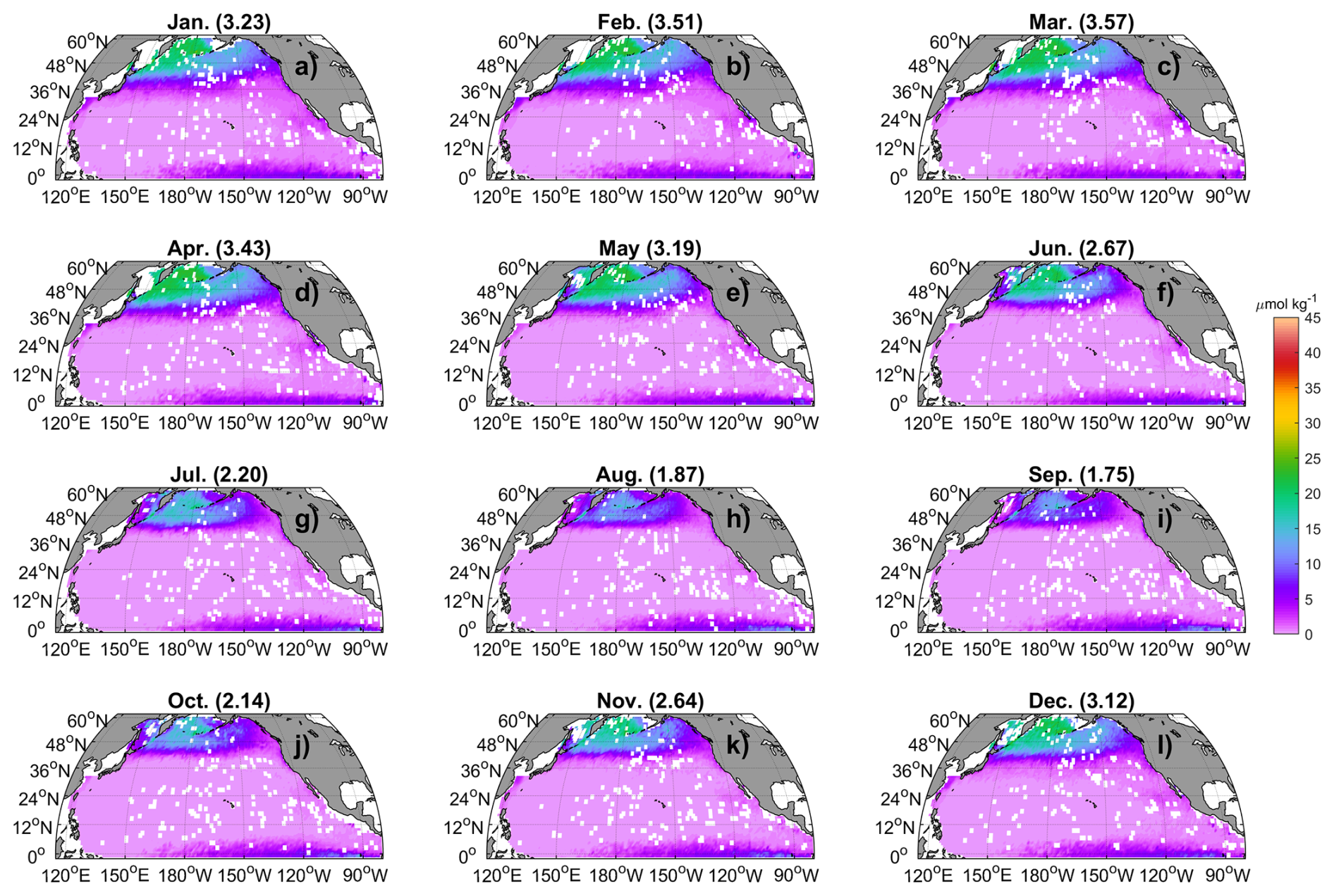
Figure 10 The monthly climatology of NO${}_x^{-}$ at 5 m in the North Pacific. Data are binned and averaged within 1°×1° grid cells. The values in the title represent the spatial mean values.

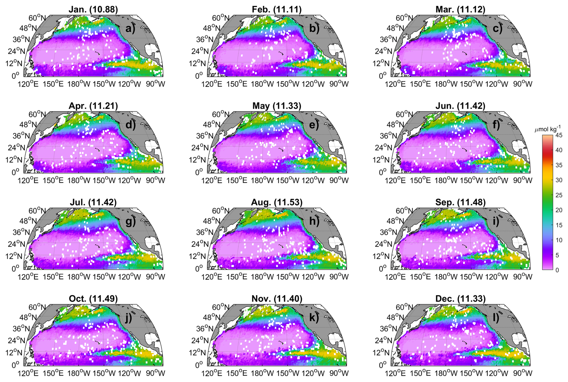
Figure 11 The monthly climatology of NO${}_x^{-}$ at 100 m in the North Pacific. Data are binned and averaged within 1°×1° grid cells. The values in the title represent the spatial mean values.

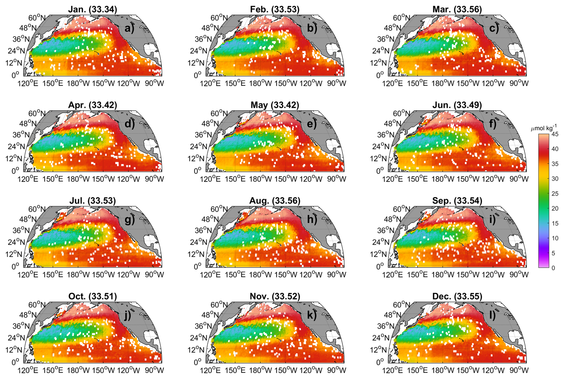
Figure 12 The monthly climatology of NO${}_x^{-}$ at 500 m in the North Pacific. Data are binned and averaged within 1°×1° grid cells. The values in the title represent the spatial mean values.

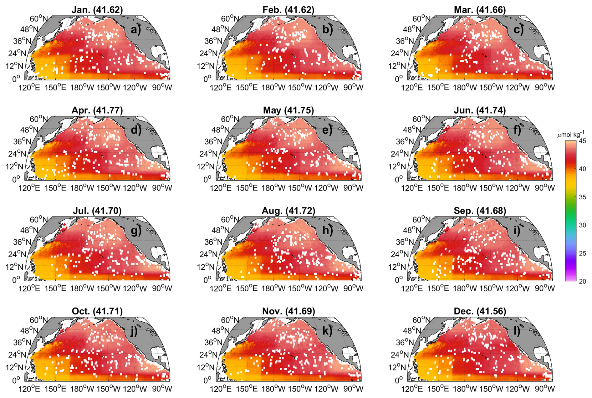
Figure 13 The monthly climatology of NO${}_x^{-}$ at 1000 m in the North Pacific. Data are binned and averaged within 1°×1° grid cells. The values in the title represent the spatial mean values.

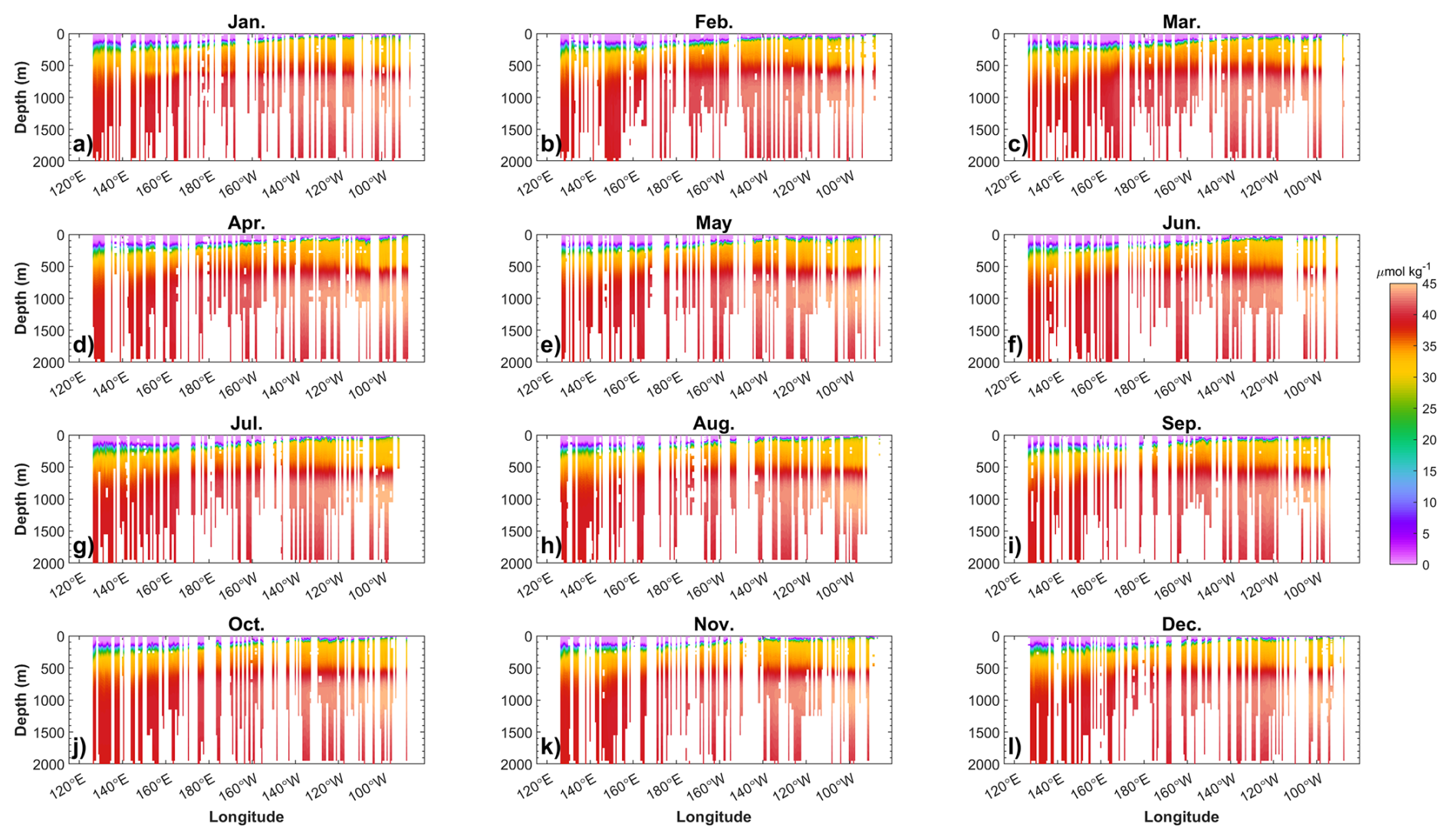
Figure 14 Zonal and monthly climatology of NO${}_x^{-}$ in the upper 2000 m at 10° N in the North Pacific. Data were binned and averaged within 1°×1° grid cells.

At 100 m, NO${}_x^{-}$ concentrations are elevated particularly in the subarctic gyre, north of the Equator, and the eastern North Pacific, while the central regions, particularly the NPSG, exhibit lower values. At 500 m, NO${}_x^{-}$ concentrations display patterns similar to those at 100 m, except that the NO${}_x^{-}$ concentrations in the western NPSG are evidently lower than those in other regions (Fig. 12). At 1000 m, concentrations in the southwestern North Pacific Ocean are markedly lower than those in other regions (Fig. 13). Below 100 m depth, seasonal variability in NO${}_x^{-}$ is minimal (Figs. 11–13). These results display patterns similar to WOA23 (Figs. S36–S44). The differences between the averaged values of these two climatologies are generally <0.7 µmol kg⁻¹ at the surface and <1.5 µmol kg⁻¹ at 100 and 500 m. The maximum differences are found in July at a depth of 500 m (Figs. 13g and S38g). In that month and layer, WOA23 shows a notably low mean NO${}_{\mathrm{3}}^{-}$ value (31.94 µmol kg⁻¹) compared to its values in other months (33.15 to 34.64 µmol kg⁻¹; Fig. S38) and compared to our climatology (33.34 to 33.56 µmol kg⁻¹; Fig. 13). This discrepancy arises because the WOA23 climatology for July features a pronounced low-NO${}_{\mathrm{3}}^{-}$ patch (down to 20 µmol kg⁻¹) within the eastern subarctic gyre, surrounded by waters with concentrations of >35 µmol kg⁻¹ (Fig. S38g). These regional differences are clearly visible in the difference maps between the two products (Figs. S45–S47). Generally, our reconstructions capture finer spatial detail, exhibit less oversmoothing, and avoid artificial “bull's-eye” patterns.

Sectional distributions of NO${}_x^{-}$ in the upper 2000 m along 10° N and 180° E were used as examples to illustrate the vertical profile distributions of nutrients within the North Pacific. At 10° N, NO${}_x^{-}$ concentrations increase from ∼0.0 µmol kg⁻¹ at the surface to ∼45.0 µmol kg⁻¹ at ∼1000 m, followed by a decrease to ∼38.0 µmol kg⁻¹ at 2000 m. NO${}_x^{-}$ concentrations increase from west to the east in the North Pacific in the upper 300 m (Fig. 14). At 180° E, in the upper 500 m, meridional NO${}_x^{-}$ concentrations increase from the equator to the North Equatorial Current (∼10° N), decline within the subtropical gyre, and then increase toward the subarctic region (Fig. 15). Generally, seasonal differences of NO${}_x^{-}$ concentrations along both sections are not evident.

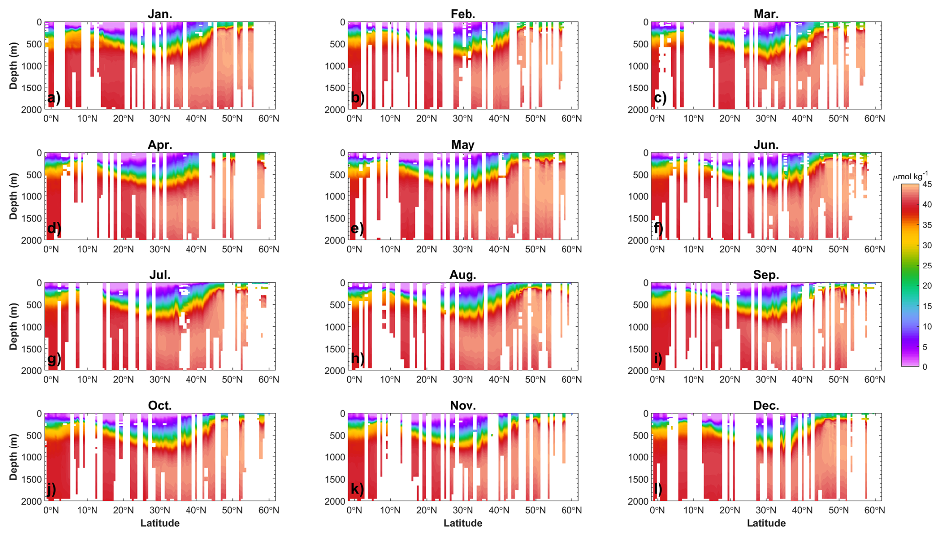
Figure 15 The monthly climatology of NO${}_x^{-}$ in the upper 2000 m at 170° E section in the North Pacific. Data were binned and averaged within 1°×1° grid cells.

3.4 Long-term variations of nutrients

We present an initial analysis of long-term nutrient changes by examining five representative regions in the North Pacific, covering the subarctic gyre, the subtropical gyre, and equatorial areas (Fig. 16). The data are binned by region, month, and depth (10, 100, 200, 300, 500, and 1000 m) for regions 1–5. As shown in Fig. 17, these time series reveal notable interannual fluctuations of NO${}_{\mathrm{3}}^{-}$ (with 2–5-year oscillations), providing a first-order view of low-frequency variability captured by the reconstruction. However, no evident long-term trend is found for nutrients. DIP and Si(OH)₄ display patterns similar to NO${}_{\mathrm{3}}^{-}$ (Figs. S48 and S49). In contrast, at depths of 200 and 300 m, NO${}_{\mathrm{2}}^{-}$ displays an increasing trend in the central NPSG and a decreasing trend in the eastern NPSG during the 1970–2005 period (Fig. S50). More sophisticated trend analyses and basin-scale integrations are promising avenues for future work based on this newly reconstructed dataset.

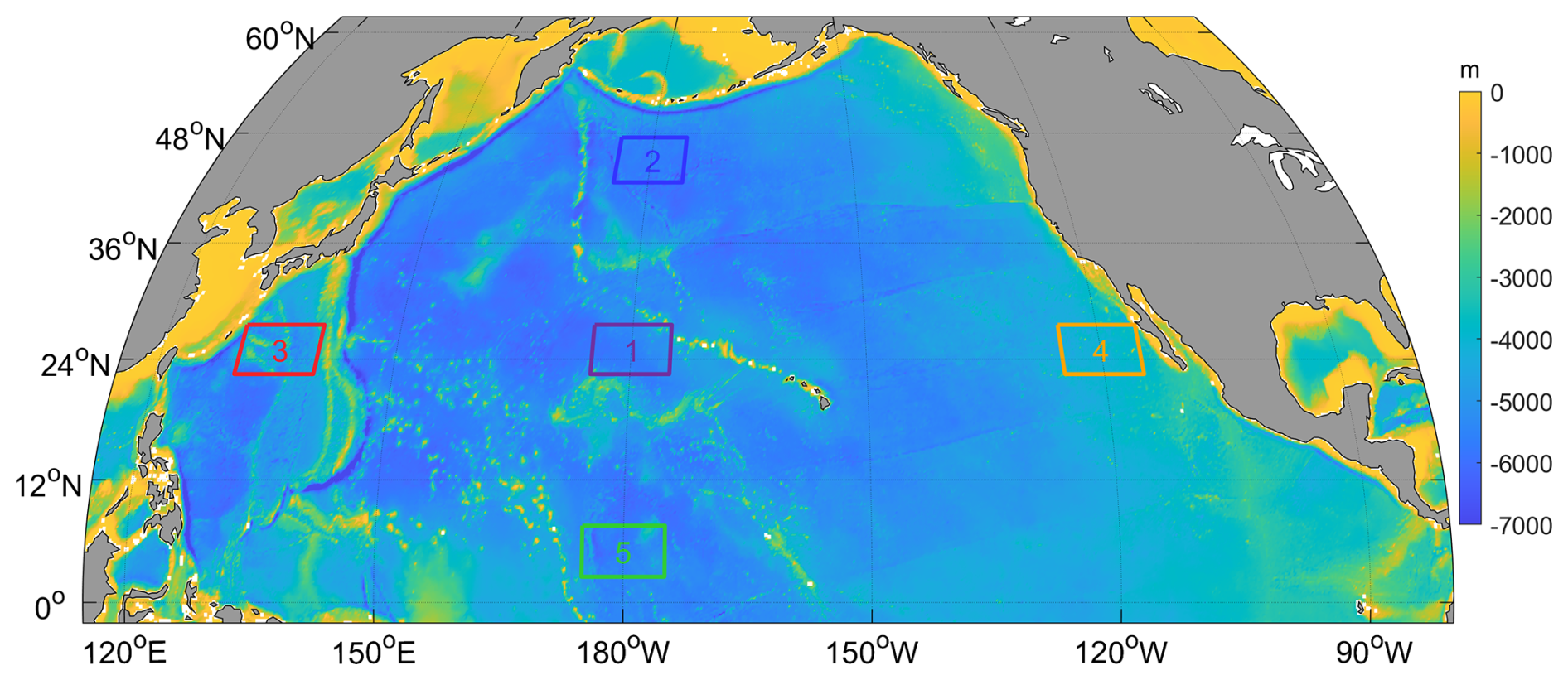
Figure 16 Locations of five representative regions for analyzing long-term nutrient variations.

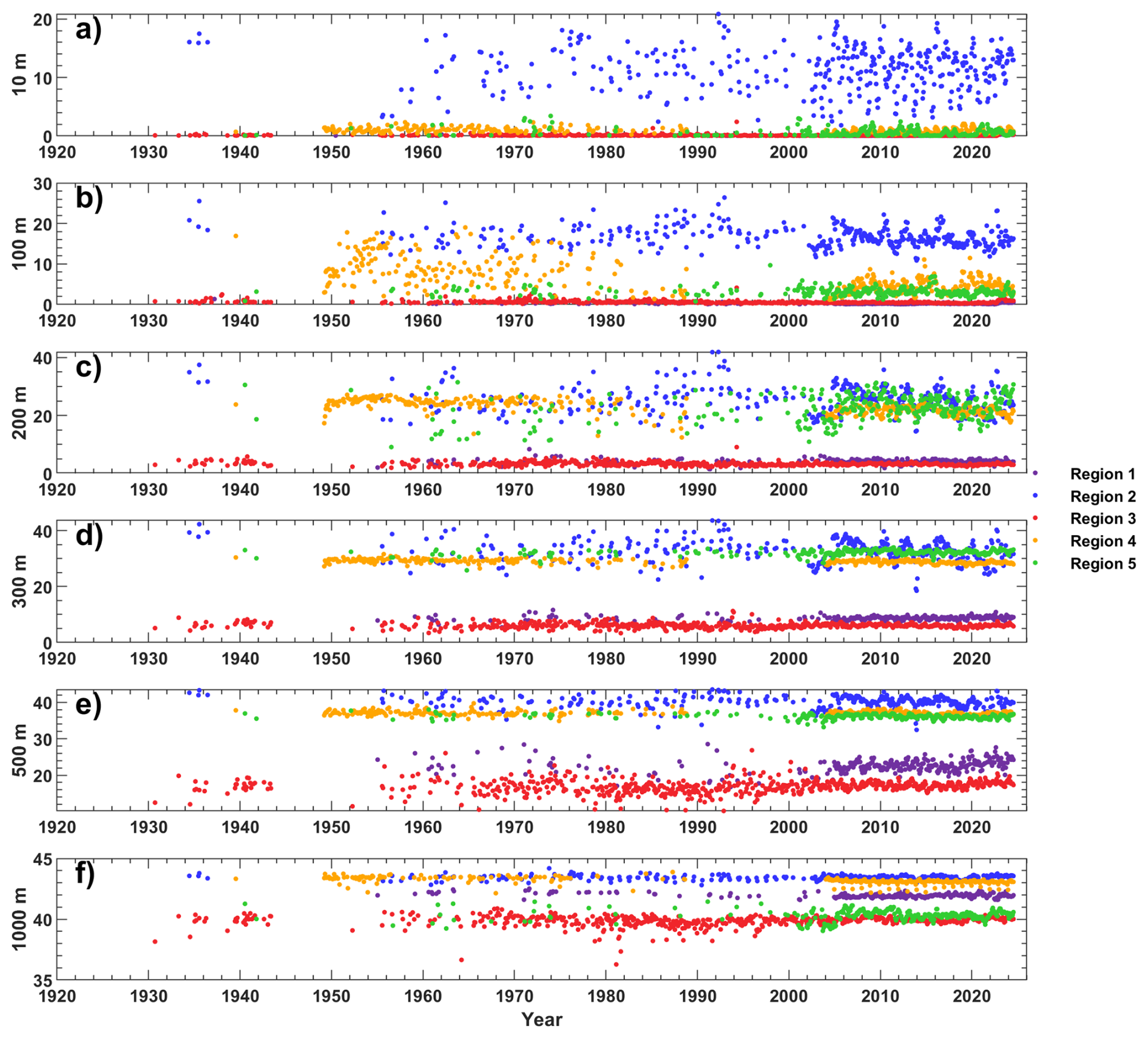
Figure 17 Time series of reconstructed NO${}_{\mathrm{3}}^{-}$ concentrations at 10 m (a), 100 m (b), 200 m (c), 300 m (d), 500 m (e), and 1000 m (f) for regions 1–5 (see Fig. 16). Data were binned by depth and region and then averaged by month.

4 Data availability

The database is freely available at https://doi.org/10.5281/zenodo.17451417 (Du et al., 2025). The files, containing the RF-, LightGBM-, and GPR-reconstructed data, are stored as text (.txt) files within a zip archive.

5 Conclusions

In this study, we applied rigorous quality control procedures to clean hydrographic and nutrient observations from CCHDO and WOD datasets. The cleaned CCHDO data were then used to train three machine-learning models to relate nutrient concentrations to spatial, temporal, and water-mass predictors. The models were applied to reconstruct nutrient concentrations from hydrographic observations collected from WOD, most of which lack direct nutrient measurements. We assessed the model performance using four data-partition strategies, and found that all models reproduced held-out data with low RMSEs. RF and GPR slightly outperformed LightGBM. The application of these models to WOD hydrography yielded 472 652 680 reconstructed nutrient concentrations across 1 920 634 stations and 35 744 cruises, spanning from 1895 to 2024. This represents a 2127- to 2393-fold increase compared to the original volume of CCHDO nutrient data. The reconstruction captured the spatial, seasonal, and interannual variations of water column nutrients in the North Pacific Ocean well. Compared to the WOA23 climatology, the reconstruction-based nutrient climatology exhibited more realistic spatial structures than WOA23. This high-quality and high-resolution nutrient dataset adds historical nutrient estimation for locations and times with solely hydrographic measurements. Additional potential applications of this dataset include: (1) investigating nutrient transport and budget in the North Pacific; (2) spinning up and validating ocean biogeochemical models; (3) assessing long-term nutrient trends driven by anthropogenic forcing and climate change; (4) investigating nutrient stoichiometric changes and their ecological impacts under climate variability. Collectively, this resource facilitates advanced studies on marine biogeochemical cycles, ecosystem dynamics, and climate–nutrient interactions.