Mapping sea ice concentration using Nimbus-5 ESMR and local dynamical tie points

As part of the European Space Agency's Climate Change Initiative, the one channel US satellite microwave radiometer Nimbus-5 ESMR (N5ESMR) level 1 data have been reprocessed to estimate global sea ice concentration from 11 December 1972–16 May 1977. The full data set is available in the CEDA Archive: https://doi.org/10.5285/8978580336864f6d8282656d58771b32 (Tonboe et al., 2025) at a grid resolution of 25×25 km² and a daily timestep. A new methodology using locally and seasonally variable algorithm coefficients called tie points has been used to calculate the sea ice concentration in radiometrically distinct ice types in the Arctic and Antarctica. Validation of sea ice concentration using Arctic sea ice charts from the US National Ice Center shows an overestimation of open-water SIC of up to 20 % where open ocean meets land and near the ice edge and an underestimation of SIC in sea ice covered regions near the ice edge, especially in the Greenland Sea. Validation also shows that local dynamical tie points (LDTP) improve the mapping of sea ice concentration for different types of ice, while estimates of the extent of sea ice are identical to the previous processing of the same data in Kolbe et al. (2024). A new set of quality control (QC) filters has been developed that discards far fewer data points (57.7 % reduction) than the filters in the previous processing. The data set therefore closes significant gaps in the sea ice concentration and sea ice extent record compared to the earlier data record. Of the 1.6 billion data points recorded by the satellite, 23.0 % have been discarded. However, 1136 d during the 1616 d period from December 1972–May 1977 are covered (at least partially). This coverage gives estimates of the mean monthly sea ice minimum and maximum extent in the Arctic and the Antarctic during this period, except for March in 1973 which is the month with maximum sea ice extent (SIE) in the Arctic and the minimum in the Antarctic.

1 Introduction

The extent of sea ice is an important indicator of climate change because sea ice affects and responds to changes in the energy balance of the Earth's surface and the ocean and atmospheric circulation (e.g., Notz and Stroeve, 2016; Masson-Delmotte et al., 2021; Moore et al., 2022; Silvano et al., 2025). Long and consistent observational records of the extent of sea ice, dating back to the beginning of the 1970s, are critical to understanding these processes and to validate models (Fogt et al., 2022; Goosse et al., 2024). For example, air–sea heat flux in the Nordic Seas, linked to atmospheric and ocean circulation and sea ice, experienced a persistent change in the late 1970s (Moore et al., 2022). The extent of Antarctic sea ice experienced a springtime drop in 2016 (Turner et al., 2017). In the mid-1970s, the extent of Antarctic sea ice also experienced a drop, which was comparable to and yet less persistent than the 2016 drop (Goosse et al., 2024).

Satellite microwave radiometer data have provided a detailed record of these recent global changes in sea ice extent (SIE) and concentration (SIC) from 1978 to today (see, e.g. Tonboe et al., 2016; Lavergne et al., 2019; Parkinson, 2019). This data record comes from a series of conically scanning microwave radiometer instruments with frequency channels near 19 and 37 GHz and dual polarization (horizontal and vertical). The first satellite in that record, launched in October 1978, the Nimbus-7, was at the same time the last mission in the very successful Nimbus satellite program. Recently, experimental satellite microwave data from the earlier missions Nimbus-5 (launched December 1972) and Nimbus-6 (launched June 1975) have been used to extend sea ice records further back to December 1972, while a gap from June 1977 to September 1978 still remains (Parkinson et al., 1987; Kolbe et al., 2024, 2025; Tellefsen et al., 2025). The data set described here is part of that effort.

The methodology developed for processing the data set in Tonboe et al. (2016) to reduce noise and achieve stability of the sea ice climate data record (CDR) when processing data from nine different multichannel instruments (Nimbus-7 SMMR, 6 DMSP SSM/I, and 2 DMSP SSMIS) is also applicable to processing historical and experimental data sets from Nimbus-5 and 6 ESMR with poor calibration (Kolbe et al., 2024; Tellefsen et al., 2025). The same methodology has also been applied to process microwave radiometer sounder data from the Nimbus-6 SCAMS instrument not traditionally used for sea ice mapping (Kolbe et al., 2025), when NASA made these data sets available at level 1 in 2016 (GSFC, 2016).

This methodology for processing these data sets first reduces the regional variability of T_B due to geophysical noise sources (wind-induced roughness of the ocean surface, atmospheric temperature, water vapor, cloud liquid water, and ice temperature) using atmospheric reanalysis data and a radiative transfer model (RTM). Secondly, the SIC algorithm is calibrated to the actual ice and open water T_B signatures measured by the instrument to avoid biases from instrument drift and calibration, inter-sensor differences, reanalysis data, RTM, and seasonal/inter-annual variations in the ice and water T_B signatures. Third, residual uncertainties are quantified using an uncertainty model (Tonboe et al., 2016). We follow those steps here.

In 2023, the ESA Sea Ice Climate Change Initiative (ESA CCI) released the Nimbus-5 ESMR Sea Ice Concentration, version 1.0 (v1.0) dataset (Tonboe et al., 2023), using the methodology of Tonboe et al. (2016) and processed as described in Kolbe et al. (2024). However, because Nimbus-5 ESMR (N5ESMR) is a one-channel instrument, there is an ambiguity between the ice type and the sea ice concentration in the v1.0 dataset. Furthermore, data suffer from drift in housekeeping data, which led the data quality control (QC) filters in Kolbe et al. (2024) to discard about half of the data. Especially the last two years of instrument operation from 1975–1977 are sparsely covered after QC. These two issues have been addressed in this new Nimbus-5 ESMR Sea Ice Concentration, version 1.1 (v1.1) (Tonboe et al., 2025) processing of the N5ESMR data by: (1) applying regional tie points and taking into account the radiometric differences between the ice types, and (2) applying QC filters that only discarded individual erroneous data points and were adapted to calibration variations.

An independent evaluation of the v1.1 dataset has been conducted by Kern (2026), comparing it with Arctic Landsat-1 high-resolution optical imagery from 1974, which showed that the statistical performance parameters are as good as those for the evaluation of modern SIC records (Kern et al., 2022).

The objectives of this study are to reprocess the N5ESMR data to estimate the extent and concentration of sea ice in both polar regions, including the uncertainties of the estimates.

2 The Nimbus-5 ESMR instrument and data

The Nimbus-5 Electrically Scanning Microwave Radiometer (ESMR) was a single channel (horizontally polarized 19.35 GHz) microwave radiometer mounted in front of the satellite. The 83 cm×83 cm phased array antenna controlled the 78 scan positions across the track, giving varying incidence angles and spatial resolution from approximately 25 km at nadir to approximately 150 km at 63° at the edges of the swath symmetrically around nadir. This across-track scanning instrument is different from the conically scanning constant incidence angle and spatial resolution microwave radiometers that followed Nimbus-5 ESMR for measuring sea ice: Nimbus-6 ESMR, Nimbus-7 SMMR, DMSP SSM/I, and modern surface sensing microwave radiometers. The orbit altitude of Nimbus-5 was ∼1100 km and the width of the ESMR swath on the Earth's surface was ∼3100 km covering both poles in 13.4 daily orbits. A combined side-lobe and incidence angle correction has been applied to the Level 1 data provided online at (GSFC, 2016). The angle of incidence correction, which we were unable to remove separately from the side lobe correction, means that the brightness temperatures (T_B) at horizontal polarization do not decrease as a function of the incidence angle, as expected for ocean and sea ice. Level 1 data have been co-located with atmospheric and surface parameters from ERA5 global atmospheric reanalysis simulations from the European Centre for Medium-Range Weather Forecasts (ECMWF) so that every T_B measurement is associated with a simulated estimate of atmospheric water vapor, total column water, air surface temperature, surface wind speed, and sea ice concentration (Bell et al., 2021). Subsequently, these data are used together with a radiative transfer model (RTM) for ocean ice and atmosphere to reduce geophysical noise in the T_B data (Kolbe et al., 2024). Because this processing step may introduce biases from the ERA5 data and the RTM, the tie points are therefore updated after the correction to reduce these potential biases.

2.1 The National Ice Center sea ice charts for comparison

The National Ice Center sea ice charts in digital format are used for comparison with the Nimbus-5 ESMR v1.1 SIC. During the period when Nimbus-5 ESMR was operated, weekly ice charts were based on satellite data (Nimbus-5 ESMR, NOAA 2, 3, 4 VHRR visual and infrared imagery) combined with aerial reconnaissance data and observations from ships (Fetterer, 2016). The different sources of information are combined in a manual analysis in the ice chart (Partington et al., 2003). Uncertainties in the sea ice concentration according to Partington et al. (2003) of ±5 % to ±10 %, arise from poor resolution of printed satellite imagery and cloud cover that obscures the surface when using VHRR data Fetterer (2016). The sea ice concentrations of the ice chart are generally higher than the sea ice concentrations derived from satellite microwave radiometer data (Partington et al., 2003). Although this comparison is not totally independent, because Nimbus-5 ESMR data are used in the ice chart creation, we have still chosen to include the comparison here.

3 Methodology

The processing of v1.1 is a direct modification of the methodology of the v1.0 product. Therefore, the methodology of Kolbe et al. (2024) is largely followed in this paper, except for the choice of quality filters (Sect. 3.1) and an additional post-processing step utilizing local dynamical tie points (LDTP) to correct the SIC predictions (Sect. 3.2).

3.1 QC filtering

The raw N5ESMR data set contains erroneous measurements as a result of instrumental flaws and calibration failure. For v1.0, Kolbe et al. (2024) used various QC filters specifically for each error type; we also follow this approach here. Although they were successful in removing most erroneous data points, the filters also removed a significant amount of valid data, especially during the latter half of the N5ESMR operation after 10 November 1974. The removal of valid data-points has been found to be the result of a systematic change in the instrument noise level, reflected in the housekeeping data used for filtering. This and other filters have been revisited here, and we have therefore created a new QC filtering scheme that relies solely on features present in the T_B data and not in the housekeeping data. The new scheme has been tested on all available swaths, and the threshold values are selected by qualitative inspection of data point distributions and outliers.

There are four types of filters in the new scheme, each targeting specific faulty patterns in the data. These are (i) value filters, where thresholds are used to discard data outside physically valid T_B intervals; (ii) pixel filters, which evaluate the validity of a pixel based on its neighbors; (iii) sweep filters that remove one or more sequential sweeps; and (iv) swath filters that detect if the entire swath is corrupt.

3.1.1 Value filter

The value filter works by simply removing pixels with values outside the range specified in Eq. (1).

$$\begin{array}{}\text{(1)}& \mathrm{90}\mathrm{K}<T_{\mathrm{B}}(i,j)<\mathrm{310}\mathrm{K}\end{array}$$

Since T_B of sea ice does not exceed 273.15 K, we could have limited the range to this, as done in Kolbe et al. (2024). However, to preserve the full distribution, including noise and poor calibration of T_Bs, we have chosen an upper threshold of 310 K. 310 K is the upper limit of the instrument dynamic range, and therefore, this upper threshold ensures that all valid data anywhere on Earth and in our areas of interest are kept.

3.1.2 Pixel filter

The pixel filter removes values that are significantly different from the local median value, as shown in Eq. (2):

$$\begin{array}{}\text{(2)}& \left|T_{\mathrm{B}}\right(i,j)-{\text{med}}_{\mathrm{3}\times \mathrm{3}}[T_{\mathrm{B}}(i,j)\left]\right|<\mathrm{75}\mathrm{K}\end{array}$$

where ${\text{med}}_{\mathrm{3}\times \mathrm{3}}\left[T_{\mathrm{B}}\right(i,j\left)\right]$ is the median of a local neighborhood of 3 by 3 pixels. The result of this filter is reminiscent of the value filter in Eq. (1), though the pixel filter also detects local errors that are still within the valid T_B range (see Eq. 1).

3.1.3 Sweep filters

The sweep filters focus on the relative difference between two consecutive sweeps, as described in Eq. (3):

$$\begin{array}{}\text{(3)}& \mathrm{\Delta }{T}_{\mathrm{B}}\left(i\right)={\text{med}}_j\left({\displaystyle \frac{T_{\mathrm{B}}(i,j)-T_{\mathrm{B}}(i+\mathrm{1},j)}{T_{\mathrm{B}}(i,j)}}\right)\end{array}$$

ΔT_B(i) is used in three different ways to remove specific patterns from the dataset;

1. If $\left|\mathrm{\Delta }{T}_{\mathrm{B}}\right(i\left)\right|>\mathrm{0.09}$, sweep i, and i+1 are removed.

2. If $\left|\mathrm{\Delta }{T}_{\mathrm{B}}\right(i\left)\right|>\mathrm{0.09}$ and the sweep i are within 25 rows from the start or end of the swath, all pixels in between are removed.

3. If $\left|\mathrm{\Delta }{T}_{\mathrm{B}}\right(i\left)\right|>\mathrm{0.06}$, $\left|\mathrm{\Delta }{T}_{\mathrm{B}(i+k)}\right|>\mathrm{0.06},k\le \mathrm{25}$, and $\text{sign}\left(\mathrm{\Delta }{T}_{\mathrm{B}}\right(i\left)\right)=-\text{sign}\left(\mathrm{\Delta }{T}_{\mathrm{B}}\right(i+k\left)\right)$, all rows between the two are removed.

The sweep filter removes most swath sections where consecutive errors occur in entire sweeps. This was implemented as the swaths often contain sections where consecutive sweeps have significantly different values compared to their surroundings.

We also discarded sweeps where more than 25 % of the data points are missing from other sweeps both before and after the current sweep (in a range of 25 sweeps). This resolves issues where swaths are affected by multiple filters, as the effects of individual filters might otherwise counteract one another.

3.1.4 Swath filter

In the Nimbus-5 data Catalogues vol. 2. (GSFC, 1972–1974) it is stated that:

Starting at 11:10 GMT during orbit 1062 (28 February [1973]) and continuing to the end of this catalog period, a malfunction reduced the ESMR instrument response to the range between 110 and 220 K of brightness temperature. Before the malfunction, the range was between 110 K and about 300 K.

For the remainder of the operation, this error appeared periodically for varying time intervals ranging from singular orbits to several months. An example of this error is shown in Fig. 1. The “stripy” pattern in the figure is the result of sidelobe and incidence angle corrections done by NASA, which warp the 220 K saturation limit to different values for each data point position across the swath. T_B for FYI are typically between 230 and 240 K, which is above the saturation limit.

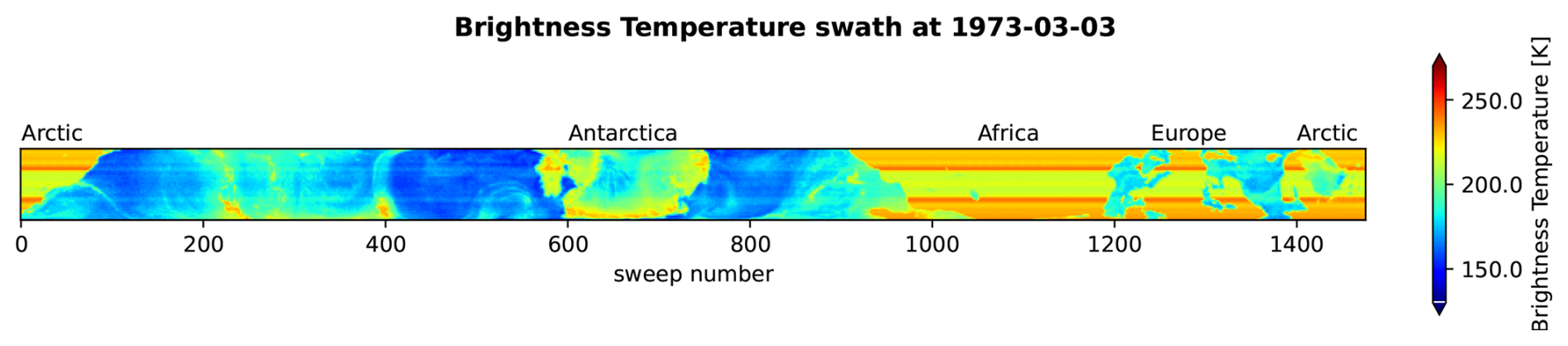
Figure 1 Example of the types of swaths the swath filter is meant to detect. In this swath, T_B over land and ice is constant along track, as the true T_B is above 220 K.

Although some information, e.g., detection of ocean/ land/ ice can still be derived from the corrupted swaths like the one in Fig. 1, the saturated T_B observations cannot be used for SIC with the methods presented in this paper. Therefore, a filtering scheme inspired by Kolbe et al. (2024) has been applied, which removes swaths with repeating values in 5 consecutive sweeps. For some corrupt swaths, repeats occur only in every other sweep; therefore, the filter has been designed to compensate for this. The filter is activated only when the erroneous pattern is detected more than 100 times in a single swath. The filter is presented in Eq. (4).

$$\begin{array}{}\text{(4)}& \begin{array}{rl}{\displaystyle }& {\displaystyle }{\sum }_{k=\mathrm{0}}^{\mathrm{5}}D(i+k)=\mathrm{0},{\sum }_{k=\mathrm{0}}^{\mathrm{5}}D(i+\mathrm{2}k)=\mathrm{0},\\ {\displaystyle }& {\displaystyle }D\left(i\right)=T_{\mathrm{B}}(i,j)-T_{\mathrm{B}}(i+\mathrm{1},j)\end{array}\end{array}$$

3.2 The Local Dynamical Tie Point (LDTP) approach

Kolbe et al. (2024) uses a one-channel SIC algorithm based on dynamical tie points for ice (T_p,ice) and water (T_p,water) to derive SIC, shown in Eq. (5), where i and j represent the spatial coordinates and t is time.

$$\begin{array}{}\text{(5)}& \text{SIC}(i,j,t)={\displaystyle \frac{T_{\mathrm{B}}(i,j,t)-T_{\mathrm{p},\text{water}}\left(t\right)}{T_{\mathrm{p},\text{ice}}(i,j,t)-T_{\mathrm{p},\text{water}}\left(t\right)}}\end{array}$$

The tie points T_p,ice and T_p,water were the mean T_B in the areas covered by the respective surface types in the ERA5 climatology and estimates of the sea ice concentration from the data itself. The 15 d running mean tie points were calculated to reduce day-to-day noise.

The problem with this approach is that it does not account for variations in T_B for different types of sea ice. The different ice surfaces show different spectral properties and spatial and temporal dependence of $T_{\mathrm{p},\text{ice}}(i,j,t)$. At 19.35 GHz, there is a significant difference between the radiometrically distinct ice type that we call first-year ice (FYI) and multi-year ice (MYI). Especially in Antarctica, the radiometric difference is caused not only by the ice age but also by the snow cover. MYI has a lower emissivity due to increased scattering from the snow and sea ice microstructure (Tonboe, 2010). For v1.0, this resulted in an SIC bias, where SIC is underestimated in MYI regions.

In our new method, $T_{\mathrm{p},\text{ice}}(i,j,t)$ is described as a function of two radiometrically distinct tie points T_p,FYI(t) (typically 235–240 K) and T_p,MYI(t) (typically 215–220 K), together with a ratio parameter $c_{\text{MYI}}(i,j,t)$. The ice tie point is a function of $c_{\text{MYI}}(i,j,t)$ as shown in Eq. (6):

$$\begin{array}{}\text{(6)}& \begin{array}{rl}{\displaystyle }{T}_{\mathrm{p},\text{ice}}(i,j,t)& {\displaystyle }=c_{\text{MYI}}(i,j,t)T_{\mathrm{p},\text{MYI}}\left(t\right)+(\mathrm{1}-c_{\text{MYI}}(i,j,t\left)\right)\\ {\displaystyle }& {\displaystyle }\times T_{\mathrm{p},\text{FYI}}\left(t\right).\end{array}\end{array}$$

This model has two parameters, $c_{\text{MYI}}(i,j,t)$ and $\text{SIC}(i,j,t)$, to predict, but there is only one observable variable (T_B). Modern microwave radiometers (e.g., SMMR, AMSR2) measure more frequencies and polarizations; and, for these, there are algorithms that utilize this multimodality to resolve the ambiguity (Comiso et al., 1997). Here, we store spatio-temporal information, which can itself be regarded as a distinct modality to resolve the SIC and ice type ambiguity. This is the logic behind the LDTP algorithm.

3.2.1 Algorithm structure

A flow chart illustrating the fully implemented algorithm is shown in Fig. 2. This implementation uses the regridded T_B from v1.0, where the RTM T_B corrections have already been applied. The algorithm is based on the assumption that $T_{\mathrm{p},\text{ice}}(i,j,t)$ is directly observable locally when SIC is constrained to 100 %:

$$\begin{array}{}\text{(7)}& T_{\mathrm{p},\text{ice}}(i,j,t)\approx T_{\mathrm{B}}(i,j,t)\leftrightarrow \text{SIC}(i,j,t)\approx \mathrm{100}\mathit{\%}.\end{array}$$

During winter, well within the ice edge, the sea ice concentration is higher than 99 % on average (Kwok, 2002; Andersen et al., 2007). The passive microwave radiometer SIC noise level is in fact much higher than the real SIC variability (Kwok, 2002). Therefore, assuming that $T_{\mathrm{p},\text{ice}}(i,j,t)$ is stable in time, this can be used as a way to find ice tie points locally even when $\text{SIC}(i,j,t)\le \mathrm{100}\mathit{\%}$. Thus, a measure of when $\text{SIC}(i,j,t)$ is 100 % is needed. For this, $T_{\mathrm{B}}(i,j,t)$ is assumed to have a low variance over time when the SIC is capped (0 % or 100 %), compared to the intermediate SIC where the T_B variance is high. This is explained by concentration fluctuations, as ice drift and melt / refreezing cause intermediate SIC, and thus T_B, to rarely remain stable over multiple days.

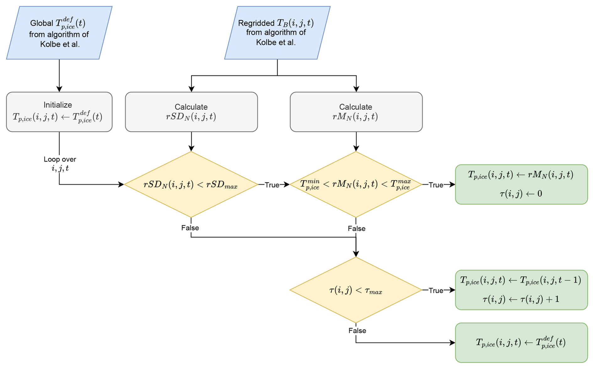
Figure 2 Flow chart for the LDTP algorithm. For the final data product, we have reprocessed the algorithm in reverse time order once to re-initialize $T_{\mathrm{p},\text{ice}}(i,j,t)$ for the first couple of days of satellite operation.

A measure of stability is therefore needed to select the local tie point. We have used the running standard deviation (rSD – see Eq. 8) to measure T_B stability. This depends on the running mean rM, which is calculated as shown in Eq. (9).

$$\begin{array}{}\text{(8)}& {\displaystyle }& {\displaystyle }{\mathrm{\text{rSD}}}_N(i,j,t)={\displaystyle \frac{\mathrm{1}}{N-\mathrm{1}}}\sum _{n=-N/\mathrm{2}}^{N/\mathrm{2}}\sqrt{\left({\text{rM}}_T\right(i,j,t)-T_{\mathrm{B}}(i,j,t+n){)}^{\mathrm{2}}}\text{(9)}& {\displaystyle }& {\displaystyle }{\text{rM}}_N(i,j,t)={\displaystyle \frac{\mathrm{1}}{N-\mathrm{1}}}\sum _{n=-N/\mathrm{2}}^{N/\mathrm{2}}{T}_{\mathrm{B}}(i,j,t+n)\end{array}$$

There are two parameters to consider for thresholding based on rSD; the period length to evaluate over, N, and the thresholding value itself rSD_max. The choice of these two parameters is discussed in Sect. 3.2.2.

$T_{\mathrm{B}}(i,j,t)$ could also be stable when $\text{SIC}(i,j,t)=\mathrm{0}\mathit{\%}$. To address this, a threshold value $T_{\mathrm{p},\text{ice}}^{\text{min}}$ is selected such that ${\text{rM}}_N(i,j,t)>T_{\mathrm{p},\text{ice}}^{\text{min}}$ for $\text{SIC}(i,j,t)=\mathrm{100}\mathit{\%}$. To also avoid erroneous tie points during the summer melt, a maximum tie point value, $T_{\mathrm{p},\text{ice}}^{\text{max}}$, is chosen. With these criteria, the evaluation of cases where $\text{SIC}(i,j,t)=\mathrm{100}\mathit{\%}$ is:

$$\begin{array}{}\text{(10)}& \begin{array}{rl}{\displaystyle }\text{SIC}(i,j,t)& {\displaystyle }=\mathrm{100}\mathit{\%}\leftarrow {\text{rSD}}_N(i,j,t)<{\text{rSD}}_{\text{max}}\wedge T_{\mathrm{p},\text{ice}}^{\text{min}}\\ {\displaystyle }& {\displaystyle }<r{M}_N(i,j,t)<T_{\mathrm{p},\text{ice}}^{\text{max}}.\end{array}\end{array}$$

By combining Eq. (7) and Eq. (10), $T_{\mathrm{p},\text{ice}}(i,j,t)$ is chosen and $\text{SIC}(i,j,t)$ is derived using Eq. (5). It is assumed that T_p,ocean is independent of space (i,j), and the tie points of Kolbe et al. (2024) are reused for open water.

The LDTP approach cannot be applied everywhere since not all areas experience $\text{SIC}(i,j,t)=\mathrm{100}\mathit{\%}$. In regions (e.g., the ocean, East Greenland current, and along the ice edge) where a stable signature cannot be established, we, therefore, use the hemispheric tie points from Kolbe et al. (2024).

Furthermore, some areas are only rarely covered by ice, and because T_p,ice changes over time, we have implemented a maximum age limit for a local tie point, τ_max, of 180 d. If a local tie point is older than 180 d, then the hemispheric tie point from Kolbe et al. (2024) is chosen. The tie point age limit was chosen to be as short as possible while still being longer than the longest periods of missing data and the melt season.

Finally, the algorithm needs an initialization period to determine which tie points to pick; therefore, we have run the algorithm forward and backward once for all dates and have picked the resulting tie points as initial values for the final evaluation; thus, we only use the tie points of Kolbe et al. (2024) for the first initialization or if τ_max is reached.

3.2.2 Parameter tuning

To select the parameters rSD_max, N, $T_{\mathrm{p},\text{ice}}^{\text{min}}$, and $T_{\mathrm{p},\text{ice}}^{\text{max}}$, we analyzed Arctic areas representing radiometrically distinct types FYI and MYI during the period 1 January 1973–1 March 1973. The manually selected areas are shown in Fig. 3. We avoided latitudes above 88° N, as the data here are derived entirely from scan positions with an incidence angle greater than 50.1° (from where incidence angles increase by more than 1° per scan position).

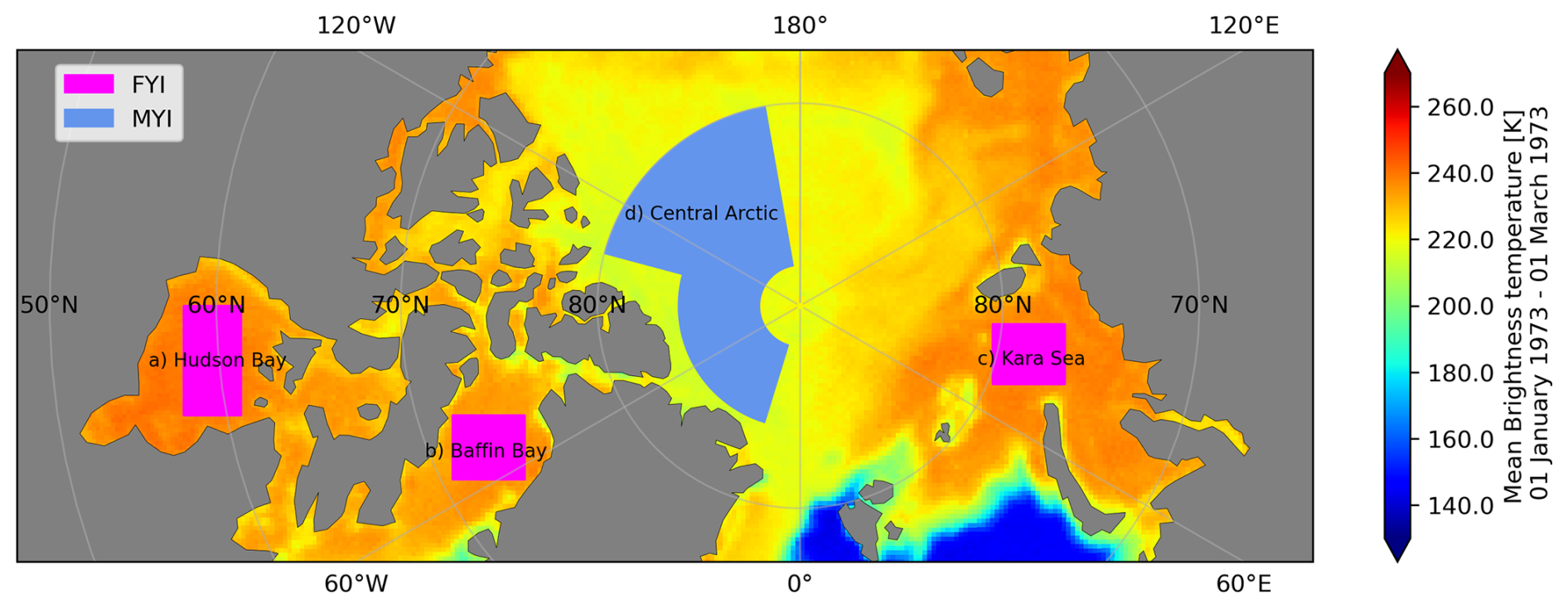
Figure 3 Areas selected as reference for parameter tuning of the algorithm. Areas containing both FYI and MYI have been selected to ensure that the algorithm is tuned to both ice types.

We found that out of a total of 142 544 observations in time and space, only 35 observations had T_B values outside the interval [205 K,255 K] (16 below and 19 above); therefore, we chose $T_{\mathrm{p},\text{ice}}^{\text{min}}\leftarrow \mathrm{205}\mathrm{K}$ and $T_{\mathrm{p},\text{ice}}^{\text{max}}\leftarrow \mathrm{255}\mathrm{K}$.

For selecting rSD_max and N, we evaluated the mean per pixel rSD for each cell across all odd values of N between 3 and 31 for the period from 1 January 1973–1 March 1973. This was done by calculating the mean rSD over time for each pixel, given each value of N. Box plots illustrating the quartile distribution of this are shown in Fig. 4. The ideal choice of parameters is not obvious. On the one hand, low rSD_max makes T_p,ice updates too infrequent, and T_B noise could mimic changes in SIC. On the other hand, too high rSD_max results in T_p,ice being updated in cases where SIC is changing, thus biasing its prediction. Furthermore, the distribution of rSD is affected by the duration of the period, N, as seen in Fig. 4. Low values of N increase the likelihood of a biased update of the tie point. Therefore, N should ideally be long. However, a too long N results in infrequent tie point updates and delayed response to changes in the ice T_Bs.

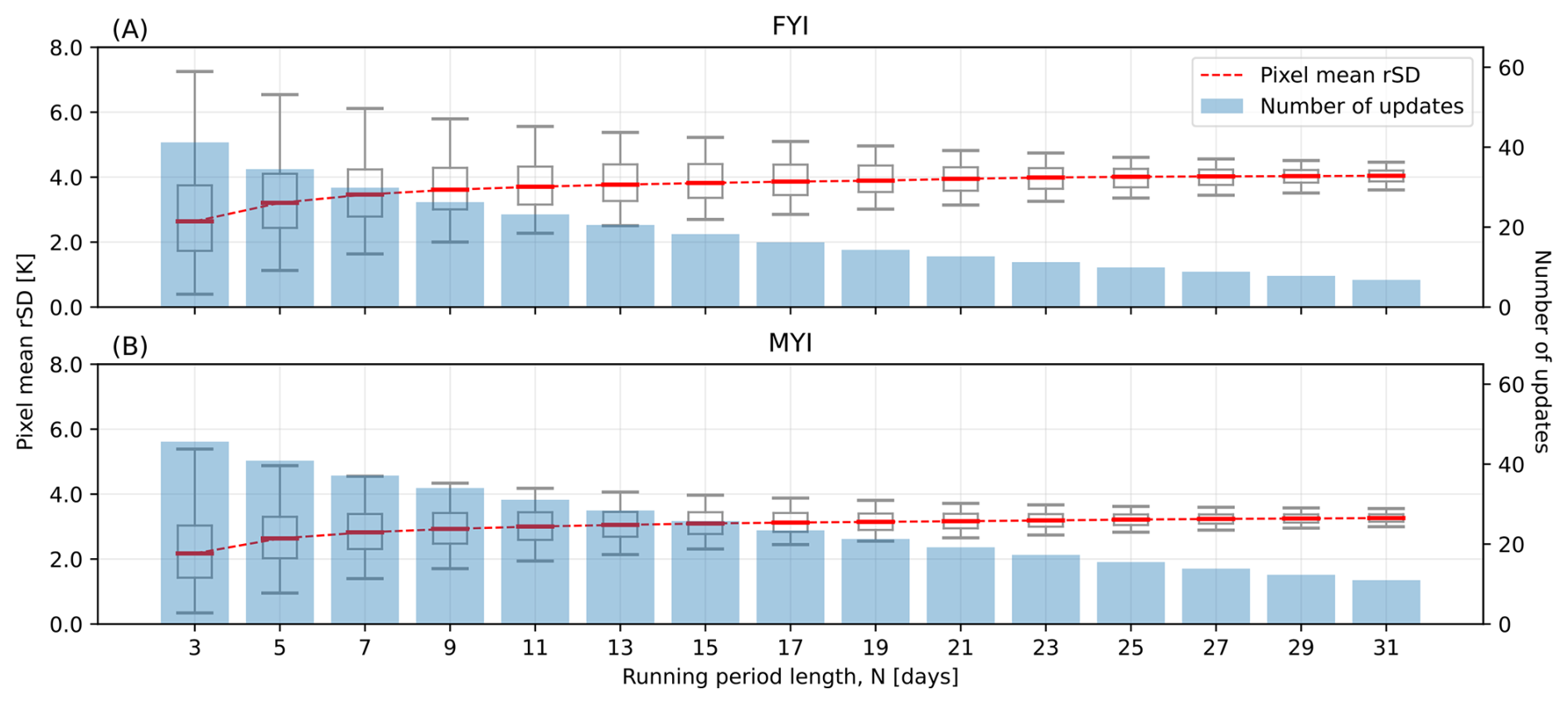
Figure 4 Per pixel mean rSD distribution for the reference areas of Fig. 3 for the period 1 January 1973–1 March 1973. Boxplots illustrate quartile distribution of pixel rSD means across time with whiskers representing minimum and maximum value. Bars illustrate the average per pixel tie point updates for the period given N, and rSD_max=3.737 K.

Based on Fig. 4, we decided to select a period length of N=15 and decrease it to a minimum of N=7 in case of data gaps. Data gaps were frequent after 14 September 1975, since Nimbus-5 ESMR data were only received every two days to prioritize resources for Nimbus-6 (Parkinson et al., 1999), and this choice of N ensures that this change does not affect update response time. rSD_max is set to 3.737, which is the FYI median value of the pixel mean rSD for N=15 (see Fig. 4a). This was chosen as FYI reflects higher rSD values in general, and rSD_max should therefore focus on distinguishing that surface over FYI. For consistency, we are using the same thresholds in the southern hemisphere.

4 Results and discussion

This section presents the effects of the new filtering scheme, and we describe the differences between the LDTP algorithm and the v1.0 algorithm. In addition, the SIC of the new and old algorithms is compared with the SIC from the National Ice Center (NIC) ice charts.

4.1 The data QC filters

An example of the effect of all QC filters (excluding the swath filter) individually and together is shown, along with the results of the old filtering scheme from Kolbe et al. (2024) in Fig. 5.

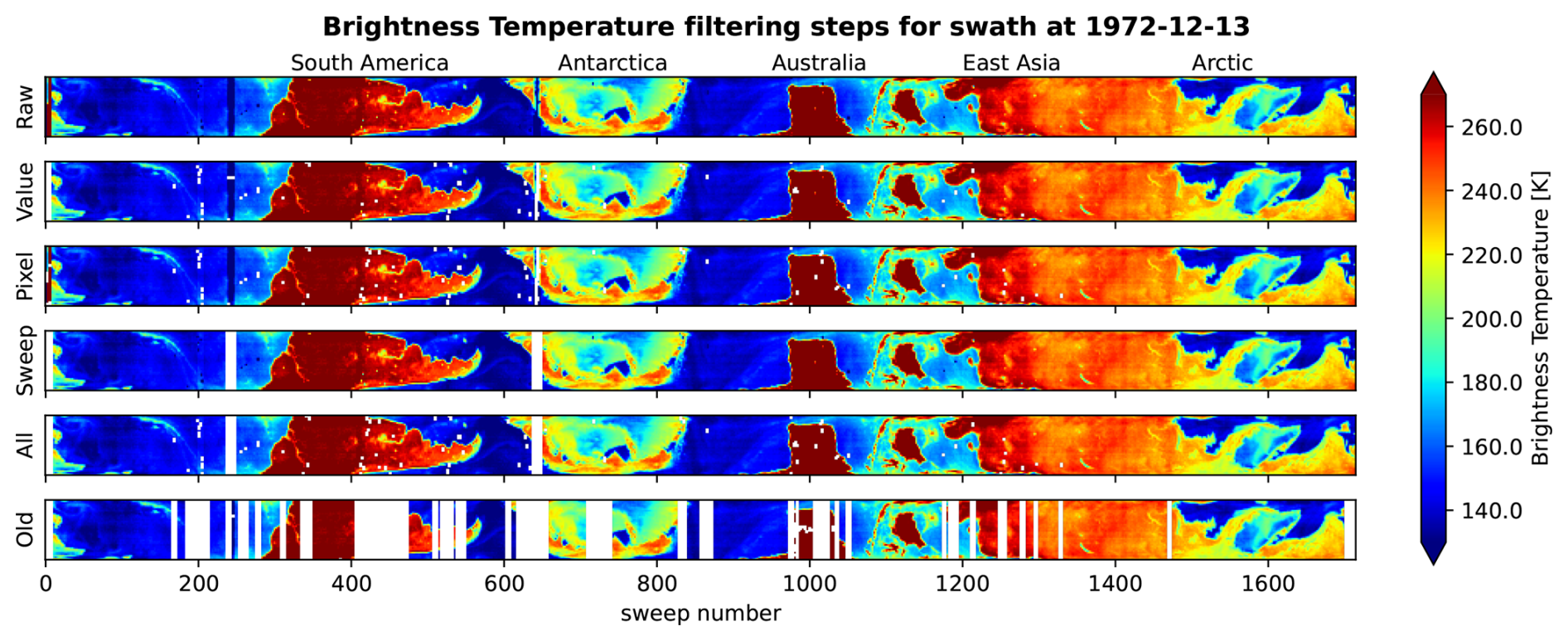
Figure 5 Display of new filters applied individually and together on a select swath (from 13 December 1972), along with the result from applying the old scheme to the same swath.

When comparing “All” and “Old” in Fig. 5, it is observed that significantly fewer valid data points are removed with the new scheme. Some “miscalibration” errors still occur, as seen around sweep 200 for “All”, but they are less prominent, and the new filters do detect some errors not detected by the old filters, e.g., near sweep 250.

In general, the old QC filters removed significantly more data than the new QC filters, especially after 10 November 1974, as seen in Table 1. The temporal pattern for data removal is further examined in Fig. 6, which compares the fraction of data removed for all swaths using the old and new filters. The figure clearly shows a pattern change around 10 November 1974 for the old QC filters, which is not seen in the new QC filters.

Table 1 Fraction of data removed by the old and the new filtering scheme, both overall, and constrained to before and after 10 November 1974.

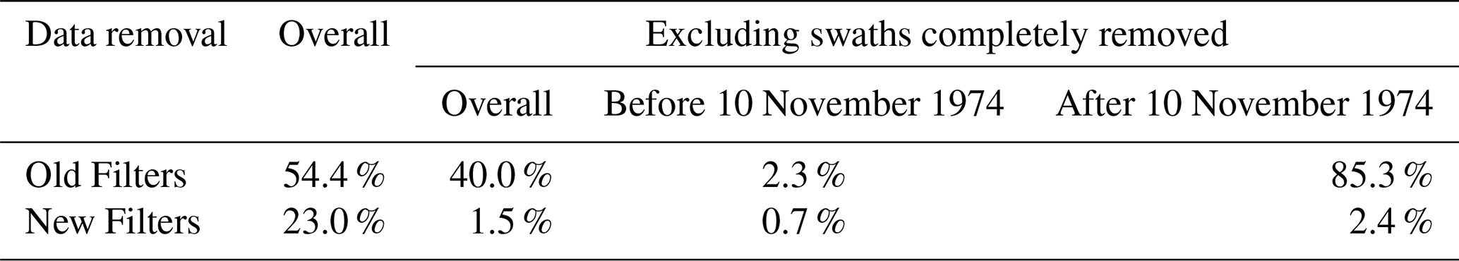
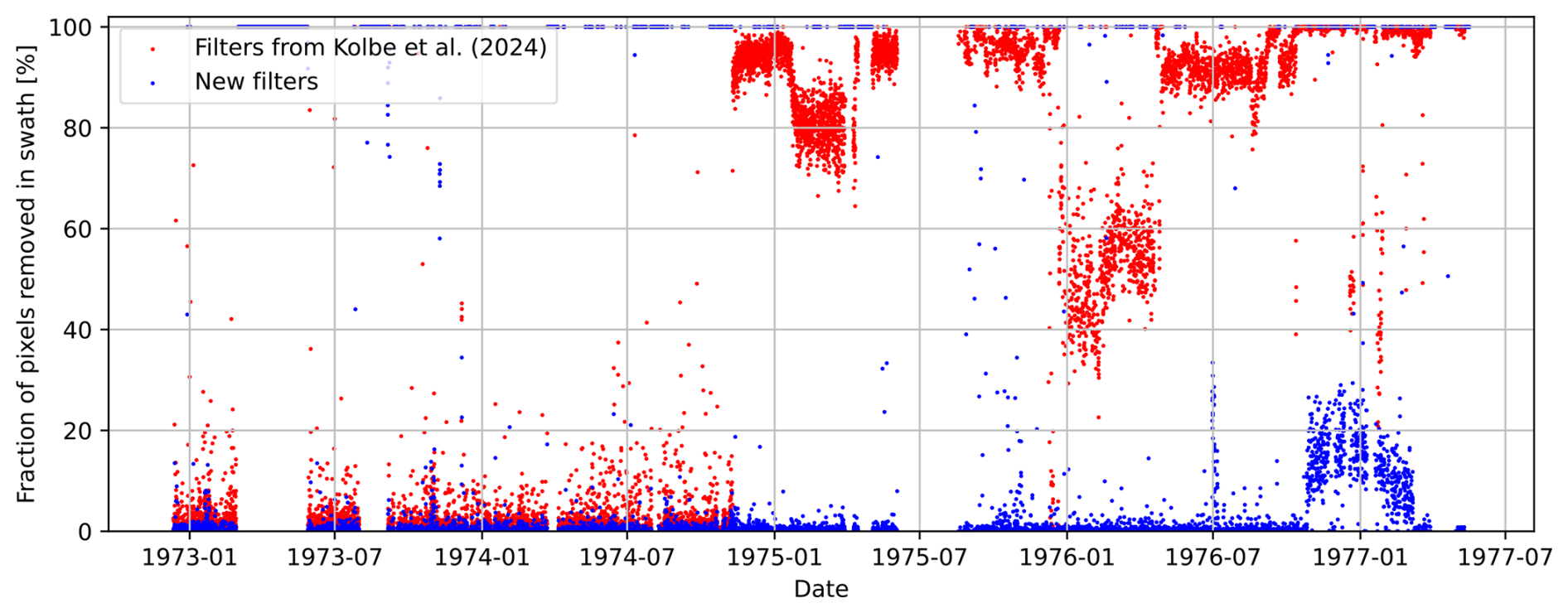
Figure 6 Amount of data being removed given the old vs. new filtering scheme. The figure shows that the old scheme in general removes more data than the new, especially following November 1974.

A peak in errors is observed around January 1977, which we found to be the result of a periodic calibration error where the mean signal changes approximately every twentieth sweep; thus, the new filter detects this error as intended.

4.2 LDTP algorithm outputs

Figure 7 illustrates the tie point and T_B differences between the Kolbe et al. (2024) and the LDTP algorithms for a pixel in area (b) Baffin Bay of Fig. 3.

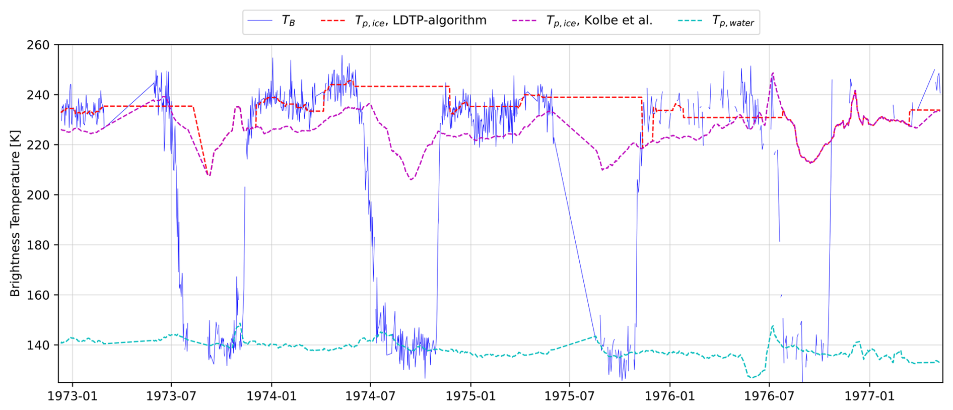
Figure 7 Average brightness temperature and tie points for a pixel in area (b) in Fig. 3. Ice tie points from both Kolbe et al. (2024) algorithm and the LDTP algorithm are shown for comparison. It is clear that the LDTP algorithm follows the ice signature of 100 % SIC more closely than the old algorithm.

Baffin Bay cycles between open water during summer and consolidated FYI during winter, as shown in Fig. 7. The Kolbe et al. (2024) ice tie points are consistently lower than the tie points of the LDTP algorithms, and the LDTP tie points follow the T_B closely. However, LDTP tie points closely follow the Kolbe et al. (2024) tie points by the end of 1973, 1976, and 1977, due to a mixture of a long melt season and missing data, which means that the age limit of the tie point is activated and the old, hemispheric tie points are used. Figure 7 shows that the new tie points in Baffin Bay replicate the T_B variability.

Figure 8 shows the spatial performance of SIC (A, G), T_B (B, H), local ice tie points (C, I), SIC standard error (D, J), rSD (E, K), and cell updates (F, L) for both the Arctic and Antarctic near the maximum extent of the ice. We see that the ice tie points for the Arctic (Fig. 8c) are distinct for FYI on the Siberian shelves, Baffin Bay and Hudson Bay, and MYI in the central Arctic. The ocean has a uniform signature, which is explained by the fact that the hemispheric Kolbe et al. (2024) open water tie point is selected. MYI is no longer distinguishable on the SIC map as in Kolbe et al. (2024). As seen in Fig. 8e, rSD is a stability measure with low values near 3 in the central Arctic, smaller regions in the Ross Sea and Weddell Sea, and high values near the ice edge. Updates are more frequent in the Arctic than in Antarctica (Fig. 8f and l), which could be due to the fact that the consolidated MYI has a lower rSD than FYI (see Sect. 3.2.2) and that there is little MYI in Antarctica compared to the Arctic. As seen in Fig. 4, MYI has a median rSD slightly lower than FYI. which means that the algorithm accepts more MYI tie points than FYI tie points. This, contrary to Kolbe et al. (2024), means that the algorithm performs better on MYI than on FYI.

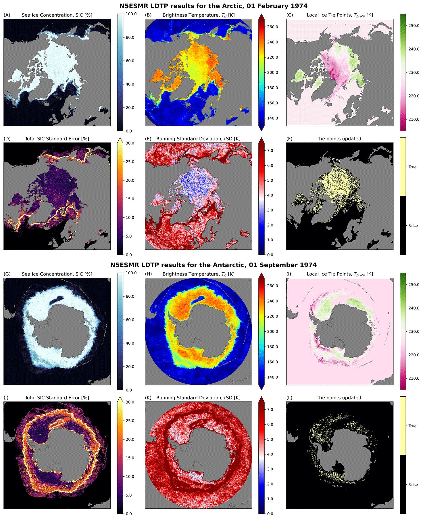
Figure 8 SIC, T_B, LDTP-based Ice tie points, SIC Standard Error, rSD and updated tie points for the Arctic (1 February 1974) and the Antarctic (1 September 1974), created using the LDTP algorithm. rSD is the running standard deviation for a 15 d period centered at the current date, while “tie points updated” are cells which tie point values have been updated for the present day.

It is clear that the requirement for the tie points, namely that the tie point signature is that of 100 % SIC, is very difficult to achieve in summer when cracks and leads remain open and melt ponds form at the surface. This issue remains even in modern sea ice concentration data sets such as those of Lavergne et al. (2019). During summer melt in the Arctic, melt ponds start to form on the surface of the ice, and at the same time, the emissivity of the snow and ice between the melt ponds changes. Eventually, late in the melt season, some of the melt ponds will melt through the floe and come into direct contact with the ocean below. However, because of the very shallow penetration depth (δ_p) of microwaves in water (δ_p<1 mm @ 19 GHz, Ulaby et al., 1986), the melt ponds will have a signature similar to that of the water in the cracks, and the leads in-between the floes and the SIC mapped with microwave radiometers are a measure of the ice surface fraction (Kern et al., 2016). In Antarctica, melt ponds are rare, but there are still melt-induced emissivity changes of snow and ice (Istomina et al., 2022). Although SIC estimates have high uncertainties during the summer, the algorithm still recovers quickly when the melt ends. Melt-induced changes in emissivity affect the SIC estimates and the sea ice area, while the SIE estimates are mainly affected by the level of open water noise (Andersen et al., 2007).

4.3 Comparison with other SIC products

The new daily v1.1 SIC (Tonboe et al., 2023) is compared with v1.0 and the Arctic ice charts from the National Ice Center (NIC) (Fetterer, 2016) in Fig. 9. We have used the zones of Fig. 3 to evaluate the biases over different surface types between the different products.

The Arctic SIC_v1.1−SIC_v1.0 difference plot in Fig. 9a shows that the LDTP algorithm correctly has SIC near 100 % over MYI, with an average difference of 9.0 % and an average difference over FYI of −2.0 %. The positive difference SIC_v1.1−SIC_v1.0 in Arctic MYI is a manifestation of the overestimated MYI tie point in Kolbe et al. (2024) and vice versa for FYI. This issue has been resolved in the new LDTP processing, as illustrated by the difference SIC_v1.1−SIC_NIC in Fig. 9c.

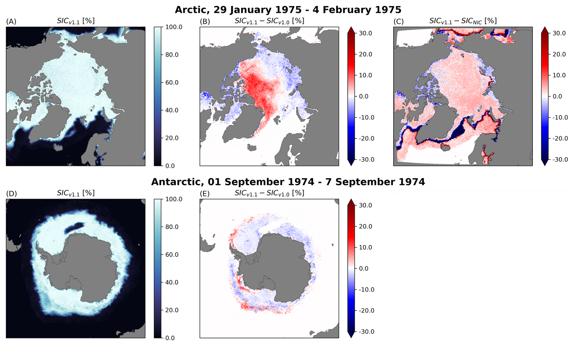
Figure 9 The top row shows Northern Hemisphere sea ice concentrations (SIC) of v1.1 (left), the v1.1 SIC–v1.0 SIC difference (middle) and the v1.1 SIC–NIC ice chart SIC difference (right), for the week covered by the ice chart 29 January–4 February 1975. An example of Southern Hemisphere SIC is depicted in the bottom row with the v1.1 SIC (left) and the v1.1 SIC–v1.0 SIC difference (middle) for the week 1. September–7 September 1974.

In Antarctica, the stable signatures, illustrated by the local ice tie points in Fig. 8i, have low values (215–220 K) near the ice edge in the Weddell and Ross Seas and in the central part of the Amundsen Sea, and higher values (230–240 K) elsewhere. The low value regions are also coincident with the regions where the SIC_v1.1 is higher than SIC_v1.0, as illustrated in Fig. 9e. This can be the result of a low rSD occurring despite less than 100 % SIC for the area, violating the main assumption of the LDTP algorithm presented in Eq. (7). A lower rSD_max might alleviate that, but it would result in even fewer tie point updates for the Antarctic. In all other regions in Antarctica, SIC_v1.1 is smaller than SIC_v1.0. In general, the running standard deviation rSD is higher in ice covered regions in Antarctica (Fig. 8e) than in the Arctic (Fig. 8k), and this affects the frequency of tie point updates (Fig. 8f and l).

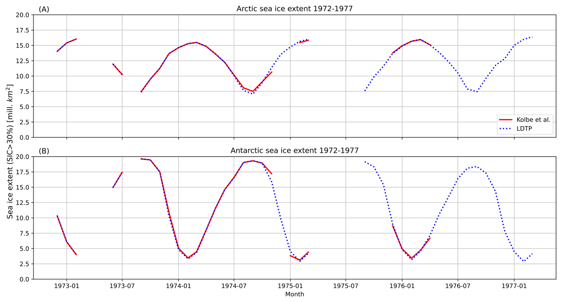
Figure 10 Monthly SIE for (A) the Arctic and (B) the Antarctic calculated with a threshold of 30 % SIC. The v1.1 product generally preserve more data compared to v1.0. Some dropouts are still observed in 1973 and 1975, and are the result of the saturation error described in Sect. 3.1.

The total SIC standard error in Fig. 8d and j is dominated by the smearing uncertainty along the ice edge. Because the zone with intermediate concentrations near the ice edge is much wider in Antarctica than in the Arctic, the zone with high total standard error (20 %–30 %) in Antarctica is much wider than in the Arctic.

In the Arctic SIC_v1.1 and SIC_NIC comparison (Fig. 9c), the differences are related to the spatial resolution of ESMR and navigational ice charts in the Greenland Sea and along the ice edge in general. Because of the coarse resolution of ESMR, even sharp ice will appear gradual in SIC_v1.1, and comparing it with the sharp ice edge in the ice chart, the differences (SIC_v1.1−SIC_NIC) will be negative over ice near the ice edge and positive over open water near the ice edge, as seen in Fig. 9c. Over the central Arctic Ocean pack ice, the SIC_v1.1 is near 100 % as expected, while the ice chart is assigned a constant SIC of 95 % as an indication that the real SIC is between 90 % and 100 % (Partington et al., 2003). Keeping this 5 % bias in mind, we find an average SIC_v1.1−SIC_NIC bias over MYI of 2.5 % and 2.9 % for FYI, which means that SIC_v1.1 on average predicts that the SIC is 2.7 % higher than the 95 % SIC from the digitized ice chart. Ice charts are not available for Antarctica. We do not have ice charts covering Antarctica and there has not been an independent study comparing the Antarctic SIC with Landsat or other high resolution optical data similar to Kern (2026). The validation of Kern (2026) was almost exclusively in Arctic FYI and the validation shows that SIC_v1.1 is virtually unbiased with a median difference of 0.0 %. We believe this is also an indication that SIC_v1.1 in Antarctica is less biased than in v1.0.

The T_B of thin ice/new ice is between ice and open water T_B and SIC (Ivanova et al., 2015; Tonboe and Toudal, 2005) and the negative SIC_v1.1−SIC_NIC difference in the Greenland Sea is probably caused by the presence of new ice (e.g., Wadhams and Wilkinson, 1999; Comiso et al., 2001; Tonboe and Toudal, 2005) or an overestimation of SIC in the ice charts (or both). The ice charts from the 1970's do not have information on ice type (except a mapping of fast ice), but an inspection of the ice charts after 1995, when ice type information became available in the charts, shows that the Greenland Sea and the Barents Sea have large fractions of new ice/ thin ice during mid-winter. In open water far from the ice edge, the SIC is overestimated compared to the ice chart due to geophysical noise that affects the SIC of the microwave radiometer (Tonboe et al., 2022).

4.4 Sea ice extent estimates

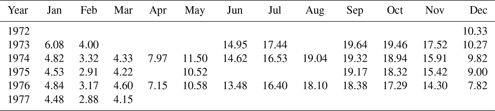
The SIE derived for both hemispheres using v1.0 and v1.1 is shown in Fig. 10. Tabular versions of the new data are found in Appendix B. The extent is calculated as the total area with an SIC greater than 30 %, and only months with more than 99 % spatial coverage in the 25 km EASE 2.0 grid are used.

As expected, the two schemes are very similar, as the LDTP algorithm of v1.1 mainly affects multi-year ice SIC, which is not detected at SIC<30 %. The main difference between the algorithms for computing SIE is the temporal coverage, which is improved by the new approach as a result of the updated QC filtering scheme. Some small differences can be seen in the latter half of 1974, likely a result of summer melt, which violates the assumptions behind both algorithms; that is, that a stable signature for 100 % SIC (the tie point) can be estimated. The summer period sea ice area and SIC estimates should therefore be used with caution.

5 Dataset

The v1.1 dataset is publicly available (Tonboe et al., 2025). It is gridded on a 25 km EASE 2.0 grid (Brodzik et al., 2012) and is available as daily NetCDF files for all dates where valid N5ESMR data are available. To maintain consistency with v1.0 and other similar SIC datasets, we have maintained the file structure, variable names, and status flags, which means that the dataset can be used as a direct replacement for v1.0. An overview of the dataset variables can be found in Tab. A1. There is a description of the status flags in Tab. A2. We have not included the LDTP algorithm specific variables: rSD, rM, T_p,ice, τ, and T_p,water to be consistent with the v1.0 data structure. However, these parameters can be derived using the available code (see below) and the corrected brightness temperatures (TB_corr) of the v1.1 dataset.

6 Data availability

The ESA Sea Ice Climate Change Initiative (Sea_Ice_cci): Nimbus-5 ESMR Sea Ice Concentration, version 1.1 dataset generated from the methods presented here, is available in the CEDA Archive (https://doi.org/10.5285/8978580336864f6d8282656d58771b32, Tonboe et al., 2025). The same dataset, along with an updated v1.0 product where only QC filters are corrected can be found at DTU data. https://doi.org/10.11583/DTU.27835929.v2 (Tellefsen et al., 2024).

7 Code availability

All data processing code is available on Zenodo (https://doi.org/10.5281/zenodo.19676225, Tellefsen, 2026). The repository includes the old and new QC filtering scheme, scripts to derive the v1.0 product with the old and new QC filtering scheme, code to upgrade v1.0 to v1.1, and scripts to create the plots of this paper (data not included).

8 Conclusions

Two issues, sea ice type and SIC ambiguity, as well as data QC in Kolbe et al. (2024), have been addressed in this new version 1.1 processing of the N5ESMR SIC data:

1. A new methodology has been developed that uses locally and seasonally variable algorithm tie points to process the N5ESMR data to retrieve the sea ice concentration in both first-year ice and multi-year ice in the Arctic and the radiometrically distinct ice types A and B in Antarctica. The new processing has resolved the SIC and the ice-type ambiguity in v1.0. On the one hand, an independent evaluation of the N5ESMR SIC dataset in Kern (2026) using high-resolution optical Landsat-1 imagery as a reference shows that the bias, standard deviation, and correlation coefficient are comparable to a similar evaluation of modern SIC CDR's (Kern et al., 2022). On the other hand, a comparison with Arctic sea ice charts from the US National Ice Center in Fig. 9 shows a bias of up to 20 % in open water near the ice edge, which is higher than the noise in modern multichannel radiometer records (Ivanova et al., 2015). However, using a SIC threshold of 30 %, the extent of sea ice is close to or identical to the v1.0 processing in Kolbe et al. (2024), as shown in Fig. 10, and this threshold avoids open water noise affecting the SIE estimates.

2. New QC filters have been developed that use 77 % of the N5ESMR data points. This is a significant improvement compared to the previous processing in which only 45 % of the data points were used. This improvement in coverage therefore closes significant gaps in the sea ice concentration and sea ice extent record, which gives estimates of the mean monthly Arctic sea ice minimum in 1974, 1975, 1976 , and the maximum extent in 1974, 1975, 1976, 1977, and the Antarctica minimum in 1974, 1975, 1976, 1977, and the maximum in 1973, 1974, 1975, 1976. The years in bold are additions since Kolbe et al. (2024). The maximum and minimum mean monthly gaps from June 1975 to March 1976 can be closed to some extent with the SCAMS microwave radiometer data onboard the NIMBUS 6 satellite (Kolbe et al., 2025). The next phase of the European Space Agency's Climate Change Initiative project will focus on the combination of satellite SIC records from different sensors in the 1970s for a more complete assessment of the global SIC and SIE.

Appendix A: Dataset parameters

Table A1 Description of the variables for the v1.1 dataset.

Table A2 Description of the status flags for the v1.1 dataset.

Appendix B: Sea ice extent

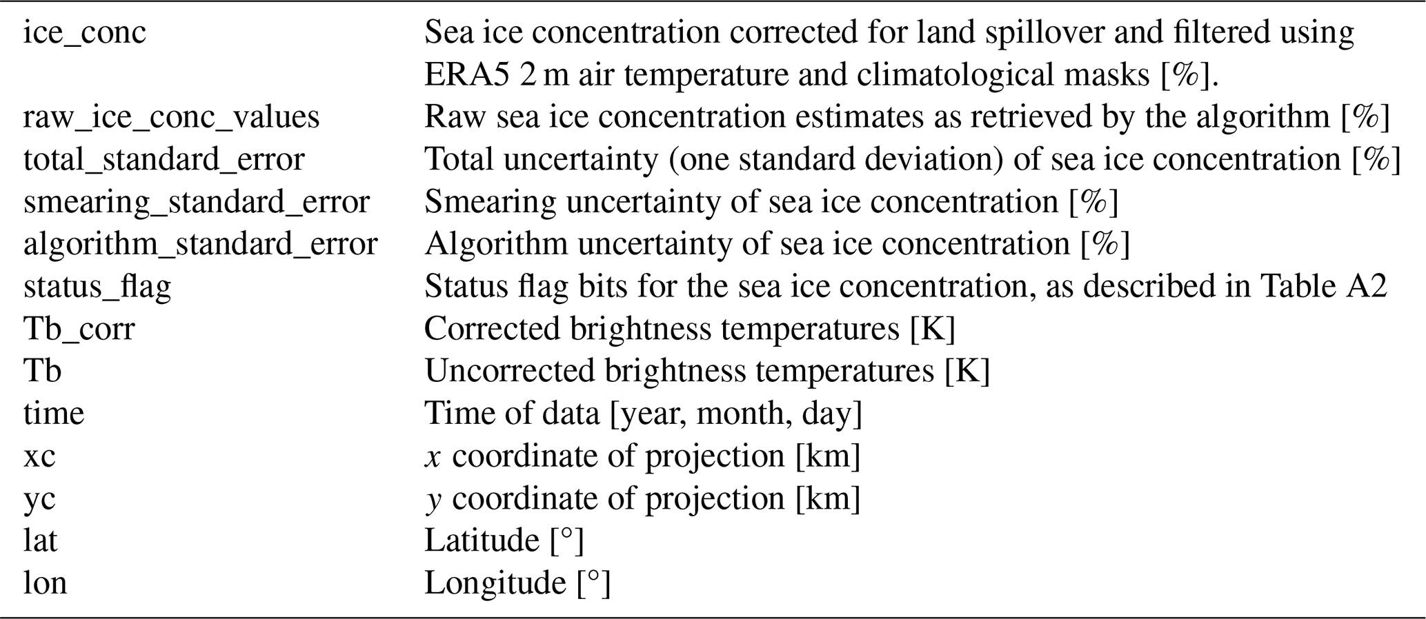
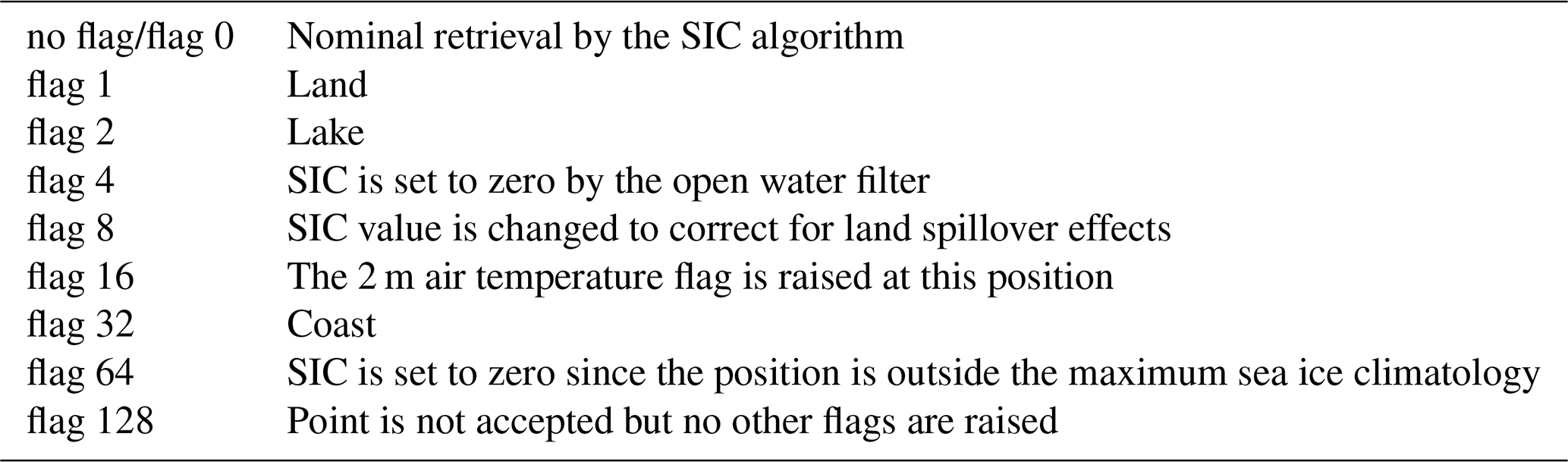
Table B1 Monthly v1.1 Arctic sea ice extent (Area with SIC>30 %) [mill. km²].

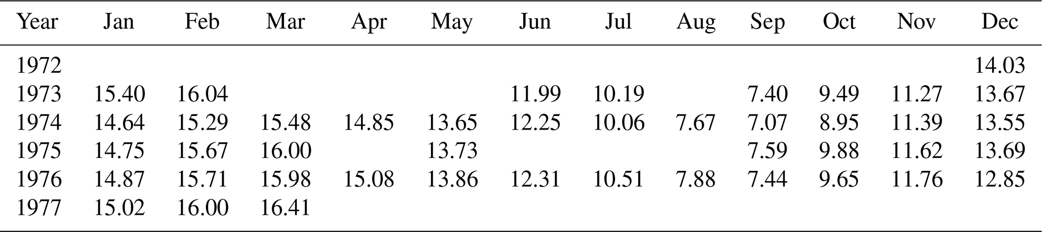
Table B2 Monthly v1.1 Antarctic sea ice extent (Area with SIC>30 %) [mill. km²].