PROMICE | GC-NET automatic weather station data

We present a new version of the PROMICE | GC-NET automatic weather station (AWS) data product, combining observations from two Greenland AWS networks; PROMICE and GC-NET. As of late 2025, the dataset integrates records from 52 active and historical AWS sites across the Greenland Ice Sheet, peripheral glaciers and land areas. This new version includes improvements in station design, sensor configuration, and data processing. Two primary station types are used: dual-boom masts in the accumulation area, and free-standing tripods with a single instrument boom in the ablation area. Data are processed with pypromice, an open-source Python package designed for standardized, transparent, and reproducible workflows, including calibration, filtering, variable derivation, and correction. The resulting products are distributed in CF-compliant NetCDF and CSV formats and include both measured and derived variables for applications in polar meteorology, climatology, and glaciology. Access is open under license CC-BY 4.0. A GitHub-based issue tracker (https://github.com/GEUS-Glaciology-and-Climate/PROMICE-AWS-data-issues, last access: 12 November 2025) supports community-driven quality control within a living data framework. The datasets are openly available at https://doi.org/10.22008/FK2/IW73UU (How et al., 2022a).

1 Introduction

1.1 Background

The Greenland Ice Sheet has contributed 0.42 ± 0.04 mm yr⁻¹ to global mean sea-level rise since 1992 (Shepherd et al., 2020), driven by changes in surface mass balance (Fettweis et al., 2017) and ice discharge (Mouginot et al., 2019; Mankoff et al., 2020). Projections indicate that the ice sheet may contribute an additional 78–175 mm to sea level during the twenty-first century, depending on greenhouse gas emission scenarios (Box et al., 2022). Regional climate models are widely used to estimate surface mass balance across Greenland, yet substantial uncertainties persist, particularly along the ice sheet margin where melt rates are highest and atmospheric conditions are more variable (Fettweis et al., 2020; Vandecrux et al., 2020). In-situ observations of accumulation, melt, and energy balance processes remain essential for evaluating model performance and improving our understanding of ice-atmosphere interactions (Hanna et al., 2020). Automatic weather stations (AWSs) play a key role in generating these observations and have delivered consistent, year-round measurements across Greenland for several decades (e.g., Smeets and Van den Broeke, 2008a; Fausto et al., 2016a).

The Geological Survey of Denmark and Greenland (GEUS) has monitored glaciers, ice caps, and the Greenland Ice Sheet since the late 1970s (Citterio et al., 2015). Early efforts relied on ablation stakes and simple automated sensors (Braithwaite and Olesen, 1989), producing valuable but spatially limited datasets. From the early 1990s onward, technological advances enabled year-round AWS operation and supported the development of several large-scale observation programmes. The Greenland Climate Network (GC-NET) was initiated at Swiss Camp in 1990 and expanded after 1995 (Steffen et al., 1996). Additional networks followed, including the K-transect stations starting in 1993 (Smeets et al., 2018), installations at Summit beginning in 2008, the SIGMA stations in northwest Greenland from 2012 (Aoki et al., 2014), and more recent installations near Kangerlussuaq (Chen et al., 2023).

Before 2007, most AWS observations were concentrated in the accumulation area, while the ablation zone – where melt dominates the mass balance – remained sparsely monitored. To address this gap, GEUS launched the Programme for Monitoring of the Greenland Ice Sheet (PROMICE) in 2007 (Ahlstrøm et al., 2008), installing 14 AWSs across seven regions (KPC, SCO, TAS, QAS, NUK, UPE, THU). PROMICE later expanded through collaborations with Austrian research groups, which provided additional stations (FRE; (Hynek et al., 2024); WEG_B and WEG_L; (Abermann et al., 2023); RED_L; (Prinz et al., 2023)), and through the Greenland Analogue Project (Claesson Liljedahl et al., 2016), whose stations (KAN_B, KAN_L, KAN_M, KAN_U) were integrated into PROMICE in 2021. PROMICE regions generally include a lower-elevation station near the ice margin and an upper-elevation station near the equilibrium line altitude, complemented in some regions by intermediate, accumulation-area, or bedrock sites. Seven stations on peripheral glaciers (NUK_K, MIT, ZAC_L, ZAC_U, ZAC_A, LYN_L, LYN_T) were installed through the Greenland Ecosystem Monitoring (GEM) programme (Abermann et al., 2019; Fausto et al., 2020; Messerli et al., 2022; Larsen et al., 2024), with Asiaq Greenland Survey operating NUK_K in long-standing collaboration with GEUS.

Table 1 Information on AWS locations and collaboration between GEUS and externally owned stations. The table lists the geographic position of each AWS (latitude and longitude in the WGS84 coordinate system), along with notes on project funding and maintenance responsibilities. While the station metadata form part of the released dataset, the funding and operational support for externally owned AWSs are provided by the respective partner institutions.

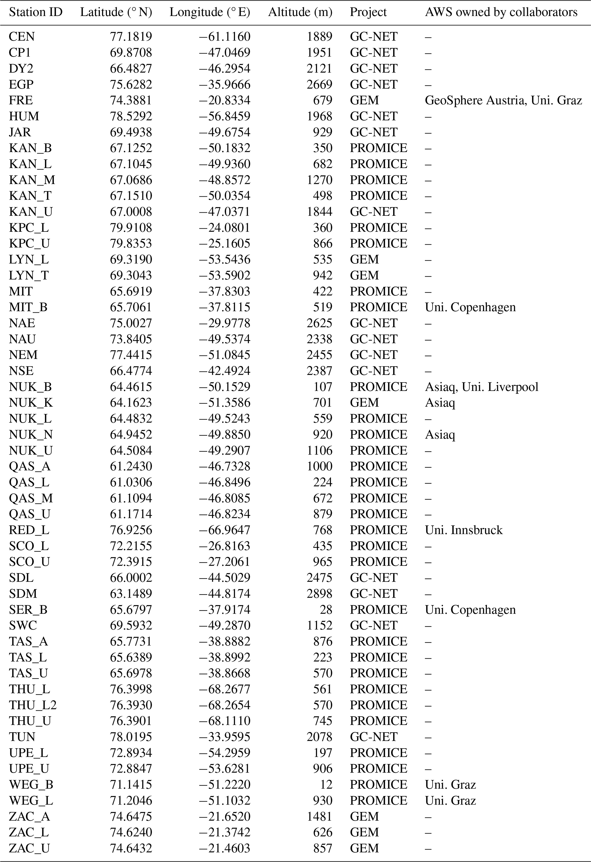
In 2021, GEUS assumed responsibility for GC-NET, integrating its sites with PROMICE operations. This transition ensured the continuation of GC-NET's legacy of high-quality data collection while leveraging our expertise and resources to maintain monitoring capabilities. In addition, a recent collaboration between GEUS and the University of Copenhagen, Department of Geosciences and Natural Resource Management (IGN) has led to the installation of two additional AWSs on bedrock near the peripheral glacier Mittivakkat Gletsjer in Southeast Greenland (SER_B and MIT_B). Lastly, the NUK_B AWS located on bedrock in the Nuuk fjord is a collaboration between GEUS, Asiaq Greenland Survey, and the University of Liverpool (Table 1). These observations support assessments of climate variability in Greenland (e.g., Poinar et al., 2024, 2025), to monitor Greenland's surface climate variability (Van As et al., 2011, 2013, 2014b), satellite and climate model validation, and participation in mass-balance intercomparison activities (Van As et al., 2014a; Ryan et al., 2017; Noël et al., 2018; Solgaard et al., 2021; Otosaka et al., 2023). This historical development provides the context for the unified dataset described in the present study.

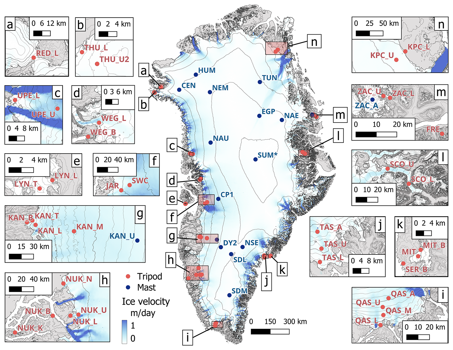
Figure 1 Map of Greenland with the latest GEUS and externally owned automatic weather station locations (Table 1).The map also shows ice velocity, confirming that all AWSs are positioned in slow-moving regions that are considered relatively safe from crevasse formation.

1.2 What is New

This study presents the latest version of the PROMICE | GC-NET AWS dataset, developed following the integration of GC-NET into GEUS operations in 2021 (Steffen et al., 1996; Steffen and Box, 2001; Vandecrux et al., 2023) and incorporating observational contributions from the GEM programme (Abermann et al., 2019; Fausto et al., 2020; Messerli et al., 2022; Larsen et al., 2024). The updated dataset builds on earlier documentation (e.g. Fausto et al., 2021) but includes an expanded network, updated instrumentation, and a harmonized data-processing workflow aligned with current standards in environmental data production (Fig. 1 and Table 1).

As of late 2025, the network now comprises 52 operational and decommissioned AWSs across Greenland, with station design tailored to local environmental conditions. Accumulation-area stations typically use single masts with two instrument booms, whereas ablation and ice-free stations use tripod structures with a single boom. Instrumentation upgrades implemented since 2021 include new fan-aspirated temperature and humidity sensors, pluviometers, tilt-correcting radiometers, CR1000X dataloggers, and digital 10 m thermistor strings. Ablation area AWSs have been equipped with high-density nickel–metal hydrate batteries to improve year-round performance. All new installations transmit hourly via the Iridium Short Burst Data system, enabling timely access to near-real-time observations.

Data processing is handled via the open-source Python package pypromice (How et al., 2023b; Python Software Foundation, 2024), which supports calibration, automated/manual quality control, and merging of data across station upgrades to ensure long-term consistency. The publicly available dataset is available in Climate and Forecast (CF)-compliant network Common Data Form (NetCDF) and comma-separated values (CSV) formats (How et al., 2022a; How et al., 2023a; Unidata, 2023; Eaton et al., 2024), in contrast to the previously used, now-deprecated space-delimited text format. Near-real-time AWS data are available via the GEUS Thredds server (https://thredds.geus.dk, last access: 12 November 2025), which provides OPeNDAP access to operational datasets (Cornillon et al., 2003; Nativi et al., 2006; OPeNDAP, Inc., 2024) with a typical latency of 10–15 min. The dataset is a living data product that updates regularly as new measurements are transmitted, processed, and incorporated into the archive.

To maximize scientific value, all data products are structured following the FAIR (Findable, Accessible, Interoperable, and Reusable) principles, promoting transparency, sharing, and long-term usability (Wilkinson et al., 2016). To enhance transparency and support community engagement, a public GitHub issue-tracking system is used to document data issues, which are tagged by station, sensor, and year and addressed in subsequent releases.

The repository is available at: https://github.com/GEUS-Glaciology-and-Climate/PROMICE-AWS-data-issues, last access: 12 November 2025. The dataset README provides up-to-date metadata, known issues, and version information (How et al., 2022b). The unified PROMICE | GC-NET dataset is available through the GEUS Thredds server (updated hourly; last access: 29 August 2025) and as a citable, manually quality-controlled monthly release at: https://doi.org/10.22008/FK2/IW73UU (How et al., 2022a). This dataset description provides a detailed overview of the PROMICE | GC-NET AWS dataset, including insights into measurements, post-processing, sensor calibration, and begins with a technical description of the AWS instruments, followed by details on the data production chain (pypromice), examples of station measurements, and concludes with a summary and outlook.

2 AWS design

The PROMICE | GC-NET AWS systems measures (1) the meteorological parameters required for calculating the surface energy budget, (2) snow ablation/accumulation and ice ablation, (3) subsurface temperature to a depth of 10 m, and (4) position by single frequency GPS. The following subsections provide detailed information on the instruments and hardware used, the AWS assembly process, the measurement frequency and accuracy of each sensor. We then present the design of the two AWS systems, including the placement of instruments, hardware, and other key considerations. Finally, we provide information on the transmission schedule and maintenance plan.

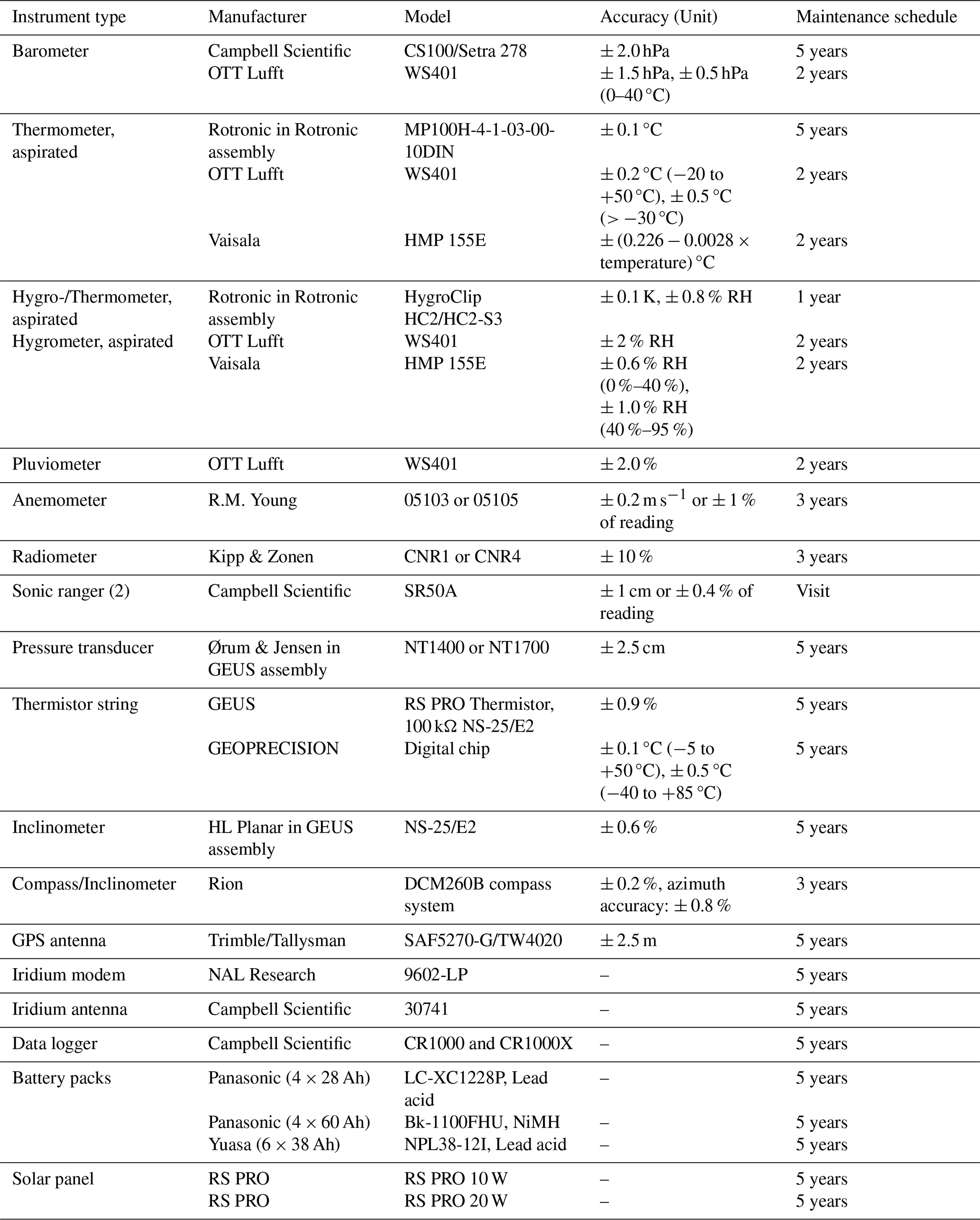
Table 2 The table summarizes the key technical characteristics of all instruments used at the AWSs, including measurement ranges, stated accuracies, operating limits, and power consumption. It also lists the planned maintenance intervals and servicing requirements for each sensor type. Full manufacturer-specific documentation for each instrument is provided in the Appendix.

2.1 Instruments and Hardware

Here, we describe the sensors and system components used in our AWS setups (Table 2), with additional technical details provided in Appendix A. In several cases, different sensor types are used to measure the same parameter. This is done to accommodate the wide range of environmental conditions across Greenland, to ensure measurement consistency across long-term records, and to select instruments that perform reliably under site-specific constraints such as extreme cold, icing, power availability, and maintenance frequency. AWS designs also differ: ablation-area stations use free-standing tripods with a single sensor boom, while accumulation-area stations use a mast with two booms positioned at different heights in the firn Sect. 2.2.1 and 2.2.2).

2.1.1 Barometer (air pressure)

Air pressure is a key atmospheric variable used to interpret weather patterns and calculate air density. Barometric pressure (in hPa) is measured in the fibreglass reinforced polyester logger enclosure using a CS100/Setra 278 barometer. The logger enclosure adjusts to ambient pressure through a pressure-compensating plug. The barometer manufacturer reports a measurement accuracy of ± 2 hPa within the −40 to +60 °C temperature range (Table 2). AWSs equipped with an OTT Lufft WS401 use an internal digital barometer based on MEMS (micro-electromechanical systems) technology and provides reliable data over a pressure range of 300–1100 hPa. The accuracy is ± 0.5 hPa within the temperature range of 0 to 40 °C, and ± 1.5 hPa outside that range.

2.1.2 Thermometer (air temperature)

Air temperature is measured to quantify surface energy balance, melt conditions, and boundary-layer atmospheric variability. In our current AWS setups, we use one of three types of thermometers depeding on the locations.

Air temperature (in °C) is measured inside a fan-aspirated radiation shield using the Rotronics setup described in (Fausto et al., 2021). The Rotronics setup refers to the combined air-temperature and humidity measurement system built around the Rotronic HygroClip probe family (HC2/HC2A-S3), installed inside a fan-aspirated radiation shield. The primary temperature sensor is a PT100 probe, which has an accuracy of ± 0.1 °C (Table 2). A secondary air temperature reading is obtained from the HygroClip temperature/humidity sensor, also housed in the aspirated shield. This sensor also has a manufacturer-stated accuracy of ± 0.1 °C but needs more frequent recalibration than the PT100 (Fausto et al., 2021).

The OTT Lufft WS401 is a compact, multi-parameter weather sensor that measures air temperature, relative humidity, air pressure, and liquid precipitation using an integrated tipping-bucket mechanism. It features a ventilated radiation shield for improved temperature and humidity measurements. The thermometer in the OTT Lufft WS401 is a capacitive sensor designed for air temperature measurement. It has a measurement range of −50 to +60 °C, with an accuracy of ± 0.2 °C at 20 °C. The sensor is enclosed in an aspirated shield.

AWSs equipped with the Vaisala HMP155E sensor measures air temperature (in °C) using a Platinum Resistance Thermometer (PT100) inside a fan-aspirated radiation shield from Rika. The measurement range is −80 to +60 °C, with accuracy varying with temperature. Specifically, for the range of −80 to +20 °C, the accuracy is ± (0.226 − 0.0028 × air temperature) °C.

2.1.3 Hygrometer (humidity)

Relative humidity (RH) is needed to estimate atmospheric moisture content, evaluate sublimation processes, and calculate longwave radiation. In the Rotronics setup (Fausto et al., 2021), relative humidity (RH; in %) is measured alongside the PT100 sensor inside the aspirated radiation shield using a HC2A-S3 (or HC2) HygroClip, which has an accuracy of ± 0.8 %.

The OTT Lufft WS401 hygrometer features a capacitive humidity sensor designed for humidity measurement, operating over a range of 0 %–100 % relative humidity with an accuracy of ± 2 % in the 10 %–90 % range at 20 °C. It is temperature-compensated and housed in an aspirated enclosure.

The Vaisala HMP155E sensor for relative humidity measurement, offering an accuracy of up to ± 1 %. It operates over the 0 %–100 % range. With an operating temperature range of −80 to +60 °C, the sensor provides fast response times, temperature compensation, and resistance to contamination.

Relative humidity is measured with respect to water, meaning calibration is performed above the freezing point. Hygrometers are typically recalibrated when possible, but in practice this occurs every 1 to 4 years. Calibration is conducted in a closed chamber at room temperature under controlled relative humidity conditions at levels of 10 %, 35 %, and 80 %. Alternatively, the instruments may be sent to the manufacturer for recalibration.

For temperatures below freezing, relative humidity is recalculated relative to ice in post-processing. To distinguish between the two relative humidities in the data products, the prior humidity (adjusted below freezing) is called “relative humidity with respect to water or ice”, whereas the latter is simply referred to as “relative humidity”. The conversion of relative humidity relative to ice is after Goff and Gratch (1946). See Table 2 for further information.

2.1.4 Pluviometer (liquid precipitation)

Liquid precipitation is monitored at stations using the OTT Lufft WS401 tipping-bucket rain gauge (in mm). Rainfall collects in a small, seesaw-like bucket that tips once a set volume (typically 0.1 or 0.2 mm) is reached, triggering a magnetic switch to record one “tip.” The total rainfall is calculated by counting these tips over time. This design performs well in most weather conditions, though regular maintenance is needed to prevent clogging or debris buildup. It is not optimal for measuring solid precipitation (e.g., snowfall) since the instrument lacks heating, which can lead to snow accumulation and delayed melting within the gauge. Nevertheless, it is adopted here as a rain gauge in a large range of conditions experienced across Greenland (Table 2).

2.1.5 Anemometer (wind speed and direction)

Wind measurements are essential for interpreting turbulent heat fluxes, drift snow processes, and station exposure. We use anemometers from the manufacturer Young. The wind speed and direction (in m s⁻¹ and degrees, respectively) measurement height, like the other measurements, has a reduced measurement height if a winter snow layer is present (Table 2). An AC sine wave voltage signal is produced by the rotation of the four-bladed propeller, and the pulse count converts to wind speed using a multiplier. According to the manufacturer, the sensor can measure wind speeds between 0 and 100 m s⁻¹, with an accuracy of ± 0.3 m s⁻¹ or 1 % if the measured value is higher than 30 m s⁻¹. Wind direction is measured through changes in the vane angle by a potentiometer housed in a sealed chamber on the instrument. The output voltage is directly proportional to vane angle wind direction and is measured between 0 and 360° with an accuracy of ± 3°. When possible, every three years the sensor is replaced and tested for drift and functionality with an “anemometer drive”, rotating the propeller shaft at a known rate. The instrument's orientation is logged and reset to “geographic north” during each maintenance visit to keep wind direction data accurate within ± 15° (although much larger station rotations have been encountered).

2.1.6 Radiometer (visual- and infrared light)

Radiometers measure the incoming and outgoing shortwave and longwave radiation needed to compute the surface energy balance. The Kipp & Zonen CNR1 and CNR4 are net radiometers (in W m⁻²), designed to measure the balance between shortwave and longwave radiation. The CNR1 is an instrument with two pyranometers and two pyrgeometers, suitable for meteorological and environmental research. The CNR4 is an advanced model offering improved accuracy, including lower thermal offset, and better longwave response. These radiometers are targeted for recalibration every three years (Table 2), however in a few cases, recalibration happens every 4–5 years.

The pyranometers, housed within hemispherical glass domes to minimize water droplet adhesion, record upward and downward shortwave irradiance between 0.3 and 2.5 µm. The manufacturer specifies a sensor uncertainty of 10 %, though practical assessments in Antarctica suggest an approximate 5 % uncertainty for daily totals (Van den Broeke et al., 2004).

The pyrgeometers measure upward and downward longwave irradiation with an estimated field uncertainty of 10 % for the CNR1 and 5 % for the CNR4. These values account for instrumental and environmental factors, including calibration accuracy and thermal offsets. Both pyrgeometers use silicon windows, sensitive to infrared wavelengths between 4.5 and 42 µm.

The radiometer data is stored in the data logger as voltage (µV) due to the unique calibration coefficients assigned to each radiometer, while all logger programs on the AWSs remain standardized for operational efficiency. During post-processing, raw sensor readings (SR_raw) are converted into physical measurements (SR_m) using the equation:

$$\begin{array}{}\text{(1)}& {\mathrm{SR}}_{\mathrm{m}}={\displaystyle \frac{{\mathrm{SR}}_{\mathrm{raw}}}{C_{\text{SR}}}},\end{array}$$

where C_SR (unit: $\mathrm{\mu }\mathrm{V}({\mathrm{Wm}}^{-\mathrm{2}}{)}^{-\mathrm{1}}$) is the sensor specific calibration coefficion provided by the manufactorer. SR_m represents either the downward or upward shortwave irradiance. Similar to shortwave radiation, longwave radiation readings are stored in the data logger as voltage (LR_raw) and later converted into physical units (LR_m) during post-processing using the formula:

$$\begin{array}{}\text{(2)}& {\mathrm{LR}}_{\mathrm{m}}={\displaystyle \frac{{\mathrm{LR}}_{\mathrm{raw}}}{C_{\text{LR}}}}+\mathrm{5.67}\times {\mathrm{10}}^{-\mathrm{8}}\cdot (T_{\text{rad}}+T_{\mathrm{0}}{)}^{\mathrm{4}},\end{array}$$

where C_LR (unit: $\mathrm{\mu }\mathrm{V}({\mathrm{Wm}}^{-\mathrm{2}}{)}^{-\mathrm{1}}$) is the sensor calibration coefficient. T_rad represents the sensor temperature recorded within the radiometer casing (in °C), and T₀ = 273.15 K.

2.1.7 Sonic ranger (surface height)

Surface height changes from snow accumulation or ice ablation are measured using the Campbell SR50A sonic ranger. The SR50A is an ultrasonic depth sensor (sonic ranger) designed for measurement of height changes, e.g. snow accumulation (Table 2). It operates by emitting ultrasonic pulses toward the surface and measuring the time delay of the reflected signal. The SR50A is durable, weather-resistant, and suitable for use in harsh environmental conditions, making it ideal for AWSs on the Greenland ice sheet. On both station designs, the sensor boom height (in m) is measured by a sonic ranger mounted approximately 0.1 m below the boom itself. For the tripod design, a SR50A is also mounted on a stake assembly drilled into the ice recording surface height changes.

Boom or stake height H_m (in m) is derived from raw sensor data (H_raw), corrected for air temperature during post-processing:

$$\begin{array}{}\text{(3)}& H_{\mathrm{m}}=H_{\text{raw}}\cdot \sqrt{{\displaystyle \frac{T_{\text{air}}+T_{\mathrm{0}}}{T_{\mathrm{0}}}}},\end{array}$$

where T₀ = 273.15 K. After temperature correction, the manufacturer-reported uncertainty for the SR50A sonic ranger (Campbell Scientific) is ± 1 cm or ± 0.4 % of the measured distance. An uncertainty assessment for sonic ranger readings, based on wintertime accumulation-free data from SCO_U, found standard deviations of 1.7 and 0.6 cm after spike removal, corresponding to uncertainties of 0.7 % and 0.6 % of the measured distance, respectively (Fausto et al., 2012).

2.1.8 Pressure transducer assembly (surface height)

Surface lowering in the ablation zone can also be measured using a pressure transducer assembly (PTA). The Ørum & Jensen NT 1700 is a robust pressure transducer designed for accurate measurement of water pressure and level in environmental and industrial applications (Table 2). It features a piezoresistive sensor element, housed in a durable stainless steel casing, and is suitable for long-term deployment. The NT 1700 offers reliable performance, stable output, and compatibility with standard data logging systems. The tripod AWSs are equipped with a pressure transducer assembly (PTA) that measures surface height changes caused by ice ablation. Originally developed in Greenland in 2001 by Bøggild et al. (2004) and later refined under PROMICE (Fausto et al., 2012), the PTA consists of a hose filled with a $\mathrm{50}/\mathrm{50}$ antifreeze-water mixture and a pressure transducer at its base. The hose is typically drilled up to 14 m into the ice, and the transducer registers the pressure from the vertical liquid column above it. A schematic showing how to construct the PTA system is provided in the appendix. Similar to the radiometer, each PTA has a unique calibration coefficient, which is why measurements (H_raw) are stored as voltage in the data logger and is converted into physical units as H_m (in m):

$$\begin{array}{}\text{(4)}& H_{\mathrm{m}}=C_{\text{PTA}}\cdot {\displaystyle \frac{{\mathit{\rho }}_{\mathrm{w}}}{{\mathit{\rho }}_{\text{af}}}}\cdot H_{\text{raw}},\end{array}$$

where C_PTA is the calibration coefficient. The constants ρ_w and ρ_af are the densities of water and the antifreeze/water solution, respectively. See Appendix Fig. A1 for further details.

2.1.9 Thermistor string (subsurface temperature)

Subsurface temperature is used to track firn and ice thermal structure, freeze–thaw cycles, and englacial processes. We have two types of thermistor strings (temperature-dependent resistor) that measure subsurface temperatures (in °C). We have a digital and an analogue type: the analogue type is designed and constructed internally, while the digital type is made by Geoprecision (Table 2, see Appendix for further details).

For sites in the ablation area, the subsurface ice temperature is measured using a 10 m thermistor string with 8 thermistors unevenly spaced. The string records temperatures at depths that may vary due to surface ablation and accumulation as seasons change through the year.

For sites in the accumulation area, the subsurface firn temperature is similarly measured using a 10 m thermistor string (digital type), but with 11  thermistors unevenly spaced to capture the higher temperature variability in the near-surface snow/firn. When installed, the top thermistor is placed at surface level, with a spacing of 50 cm to the next down to 3 m depth, then a spacing of 1 to 4 m depth, followed by 2 m spacings down to the bottom thermistor at 10 m depth. The thermistor string is inserted into a standard 32 mm (outer diameter) polypropylene pipe (PP), commonly used for sewer water and consisting of 6 × 2 m pieces, allowing for a 2 m extension above the snow surface. The PP pipe system is sealed at the bottom and a custom-made cap allowing passage of the cable is placed at the top end, providing a waterproof system with the thermistor string extended in a relatively narrow air-filled pipe. The PP pipe is usually reinforced with a stake for structural support and a thin bamboo pole is attached as an extension at the top to help locating the system if the snowfall exceeds the height of the PP pipe before next visit.

2.1.10 Compass/Inclinometer

Tilt and orientation measurements (in degrees) help correct radiation and wind data for boom inclination or rotation. We use two types of inclinometers. HL Planartechnik GmbH manufactures a series of tilt sensors designed for measuring angular displacement. The NS-25/E2 inclinometer, for example, consists of a flexible circuit that can be integrated into different measurement systems and provides an analog voltage output proportional to tilt. The Planar inclinometer measures the tilt (in degrees) both across (left-right) and along (up-down) the sensor boom, which is interpreted as tilt-to-east and tilt-to-north when the sensor boom is oriented north-south. The inclinometer's voltage readings (Tilt_raw) are converted into Tilt_m in degrees using the following equation:

$$\begin{array}{}\text{(5)}& \begin{array}{rl}{\mathrm{Tilt}}_{\mathrm{m}}=& \mathrm{21.1}\cdot \mathrm{|}{\mathrm{Tilt}}_{\mathrm{raw}}\mathrm{|}-\mathrm{10.4}\cdot \mathrm{|}{\mathrm{Tilt}}_{\mathrm{raw}}{\mathrm{|}}^{\mathrm{2}}+\mathrm{3.6}\cdot \mathrm{|}{\mathrm{Tilt}}_{\mathrm{raw}}{\mathrm{|}}^{\mathrm{3}}\\ & -\mathrm{0.49}\cdot \mathrm{|}{\mathrm{Tilt}}_{\mathrm{raw}}{\mathrm{|}}^{\mathrm{4}},\end{array}\end{array}$$

where all constants were determined in-house using. The constants were determined using a separate inclinometer by deriving a best-fit polynomial relationship between the measured voltage and the corresponding measured tilt.

The Rion compass was chosen to replace the HL Planar tiltmeter in our AWS systems. It uses magnetic field sensors to determine azimuthal orientation, providing accurate and reliable heading (tilt) data for applications that require precise directional alignment, such as measuring downward shortwave irradiance and wind direction (see Table 2).

2.1.11 GPS (AWS position)

Since their inception, all AWSs have been equipped with a single frequency GPS that records site position and position metrics hourly. The same technology has been applied to GC-Net stations starting in 2020 for the SWC site and in 2021 onward for an increasing number of the GEUS carry-forward GC-Net sites. The GPS antenna and the receiver, which is part of the Iridium 9602-LP modem, are housed inside the data logger enclosure. The receiver is a NEO-6Q model, operating at 1575.42 MHz (L1), with 16 channels and C/A code. Its accuracy is reported to be within 2.5 m (Table 2). The manufacturer states the the vertical accuracy is typically 1.5–2 times worse than the horizontal. Implicit in the single frequency measurements is the use of the EGM96 geoid to obtain orthometric height a.k.a. elevation above mean sea level. See also AWS position in the post-processing section for more information.

In the AWS configuration, the GPS receiver is activated for one minute before each Iridium transmission attempting to acquire position. The coordinates with the lowest horizontal dilution of precision is saved to memory.

The single frequency GPS can produce relatively noisy data and suffer from occasional data gaps. For the users' convenience, we distinguish between these direct GPS measurements, called gps_lat, gps_lon, gps_alt, and our best estimate of the station position at all time step, simply called lat, lon, alt derived in post-processing (see Sect. 4.1).

2.1.12 Data logger and satellite modem (local data storage and transmissions)

CR1000X is a rugged, low-power data logger from Campbell Scientific, ideal for long-term monitoring in harsh environments. It offers faster processing, more memory, and improved analog precision compared to the CR1000, along with USB, RS-232, and Ethernet connectivity. These upgrades enhance data acquisition efficiency, reliability, and flexibility.

The NAL Research 9602-LP modem is a low-power, compact device designed for reliable long-range communication. It uses Iridium satellite connectivity, providing global coverage for data transmission. The modem supports Iridium Short Burst Data (SBD), which is a communication protocol designed for sending small amounts of data. It is optimized for low-bandwidth applications that need to transmit short bursts of data, such as sensor readings, GPS locations, or status updates. Iridium SBD enables reliable communication in areas without cellular coverage.

2.1.13 Batteries and solar panels (power)

We use two types of batteries for AWS power:

• Lead-acid batteries are known for their ability to supply high surge currents, cost-effectiveness, and robustness in harsh environments (Table 2). Although their energy density is lower compared to more advanced battery chemistries, they offer consistent performance over a wide temperature range. In a controlled freezer test, we evaluated lead-acid battery performance and found that while charging below even −40 °C is feasible, only a limited amount of energy is stored; nevertheless, they remain a reliable power source under extreme low temperatures.

• Nickel-metal hydride (NiMH) batteries are also rechargeable but with higher energy density and reduced environmental impact compared to conventional lead-acid batteries. NiMH batteries exhibit relatively stable capacity across a range of temperatures; however, their performance becomes critically impaired at temperatures below −40 °C, where electrochemical activity ceases. In a series of controlled freezer tests, we evaluated NiMH battery performance at various subzero temperatures and confirmed that they remain a reliable power source down to approximately −40 °C.

For the reasons above, lead-acid batteries were chosen for high-elevation/far-North GC-NET sites at risk of temperatures below −40 °C, despite their lower energy density compared to the NiMH batteries.

RS PRO solar panels are high-efficiency photovoltaic modules designed to convert sunlight into electrical energy. These panels are made of either monocrystalline or polycrystalline silicon. RS PRO solar panels are known for their robust construction, suitable for harsh environments.

2.2 Automatic weather station design

The station designs differ between the ablation and accumulation areas due to variations in surface dynamics and logistical constraints. In the ablation area, the tripod stands on the ice and moves downward as the ice melts, keeping the sensor boom at a constant height above the surface. This design allows accurate surface-level measurements with only one sensor boom. During winter, temporary changes in surface height from snow accumulation are monitored using a sonic ranger mounted on the boom. In contrast, the accumulation area experiences continuous changes in surface height due to ongoing snowfall and snow compaction, making it harder to define a stable reference level. To accurately calculate meteorological gradients in this environment, a second measurement level is desirable. Additionally, practical considerations influence the designs: stations in the ablation area are often transported by helicopter, which often has limited cargo capacity, making compact, single-level setups preferable. In the accumulation area, larger two-level stations have been delivered by ski-equipped DHC-6 Twin Otter fixed-wing aircraft, which can carry bulkier equipment. A common feature of the AWS locations is that they are situated in slow-moving regions considered relatively safe from crevasse formation (Fig. 1).

2.2.1 Accumulation area design: Mast with two measurement levels

The GC-NET mast configuration is a two-boom system, designed for accumulation area deployment. The two booms on the mast allow for vertical profiling of the near-surface boundary layer air temperature, wind speed & direction and humidity. The historical GC-NET mast configuration, originally deployed at 18 sites starting in 1995 as described in Steffen and Box (2001) and Vandecrux et al. (2023), consisted of a 4” diameter aluminum tube with a $\mathrm{1}/\mathrm{4}$” wall thickness, providing a very stiff, but relatively heavy mast. Extending the mast thus required a tripod crane.

To enable a more light-weight system that would not require a crane, it was decided to investigate alternative mast solutions. The first light-weight alternative, deployed in 2021, was based on a 48 mm diameter titanium tube, fitted with two titanium booms. These tubes turned out to be too flexible for stable mounting of instruments, despite being anchored with 3 mm braided stainless-steel wires and reinforced with wooden poles inside. The second version, which has subsequently been deployed at all accumulation area sites, re-introduced the original outer mast diameter of 100 mm and aluminium, based on a combined analysis of weight, rigidity and usability of titanium, steel, aluminium and carbon fibre, respectively. To meet the weight requirements, the wall thickness of the 100 mm aluminium mast was reduced to 3 mm. Apart from reducing the weight of the mast itself, the number of the booms carrying the instruments were reduced from 5 to 2, with the two booms positioned orthogonally, 1250 mm apart on the mast. Additionally, the choice of a more light-weight construction has enabled a field team of four to raise a fully instrumented mast without the use of a tripod crane and winch, further reducing the total weight to be carried on the airplane.

However, the light-weight construction has also required a positioning of instruments, solar panel and logger box that could potentially reduce the quality of the measurements, as they are more closely spaced than previously, increasing the risk of shading and turbulence. Similarly, the orthogonal position of the two booms provides different conditions for the two levels of wind measurements in terms of down-wind turbulence from the measurement frame.

Despite these potential issues, introducing a more light-weight mast structure has been deemed necessary in order to provide capacity for additional personnel (generally 4–6 people), regular transport of battery boxes, tools and replacement sensors, and equipment.

Figure 2 Schematic of an accumulation area design AWS.

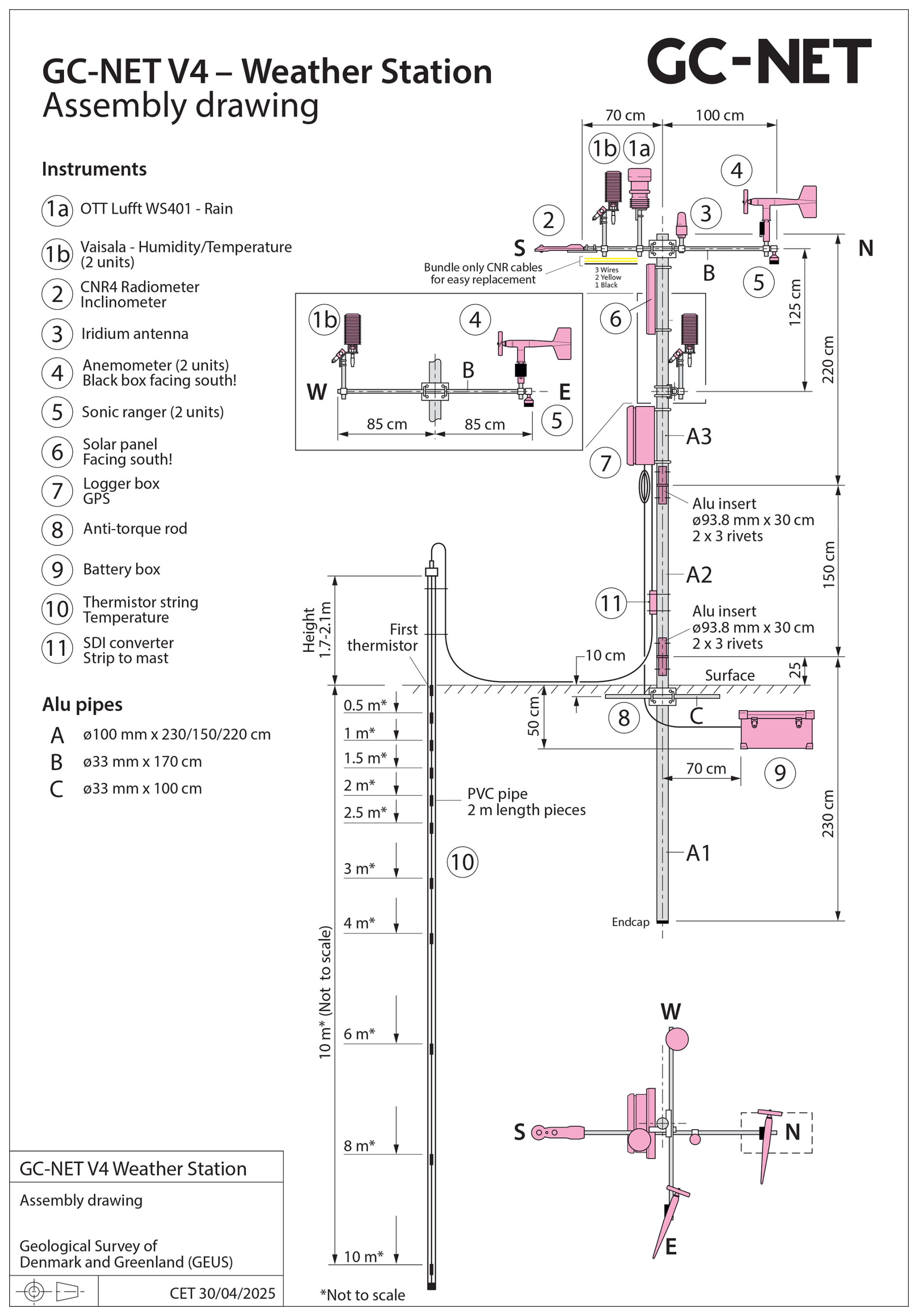
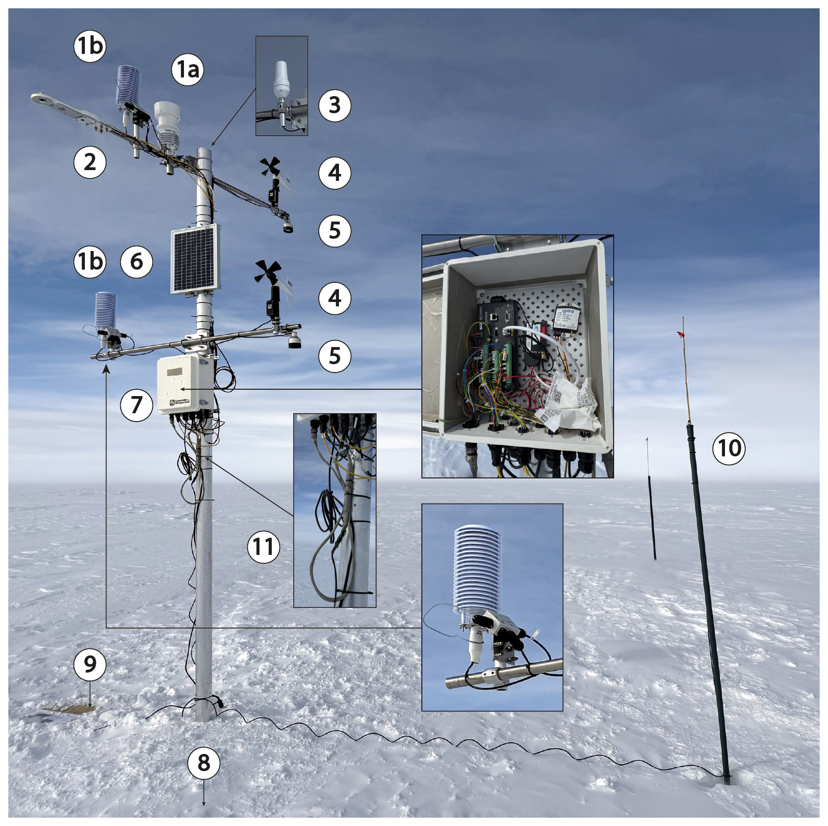
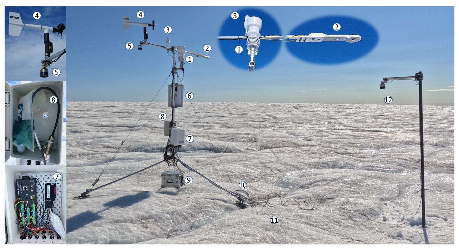
Figure 3 Photo of an accumulation area design AWS NAU photografed on 10 May, 2025. Numbering corresponds to Fig. 2. Credit: Andreas P. Ahlstrøm.

Figure 2 illustrates the schematic of an accumulation area AWS, and Fig. 3 gives and in-situ impression from the field. Liquid precipitation is measured using a OTT Lufft WS401 sensor (1a), while humidity and temperature are recorded by a Vaisala sensor (1b). Visual- and infra light is measured by a CNR4 radiometer (2), which is equipped with with an integrated inclinometer/compass (2). Wind speed and direction are recorded by two anemometers (4), and snow height is measured by two sonic rangers (5). Power is supplied by a south-facing solar panel (6), connected to a battery box (9). Data acquisition and positioning are handled by a GPS and a logger box (7). Structural stability is ensured by an anti-torque rod (8) and a thermistor string (10) is drilled into the firn measuring temperatature at 11 different levels.

The standard accumulation area mast structure consists of 6 aluminium tube pieces as shown in Figs. 2 and 3:

1. A lower part with a plastic cup in the bottom, length 230 cm.

2. A middle part, referred to as the extension part, length 150 cm

3. An upper part where all instruments and boxes are attached to, length 220 cm

4. Two aluminium inserts as assembling parts, length 30 cm, outer diameter of 93.8 mm with a short length of 2 mm of slightly larger diameter where the mast pieces meet in the middle.

5. A one metre aluminium tube of similar type as the booms, fastened to the mast just below the snow surface at first installation to ensure that the mast does not rotate.

A mast and an insert are fastened using 3 rivets (5 mm) separated by 120°. The accumulation area mast design makes it possible to always bring down the instruments for routine maintenance and rotation, without the use of a crane.

Figure 4 Schematic of an ablation area design AWS.

Figure 5 QAS_M ablation area AWS photographed 1 September 2024 on the Greenland ice sheet. Instrument numbering corresponds to Fig. 4. Credit: Jason E. Box.

2.2.2 Ablation area design: Tripod with one measurement level

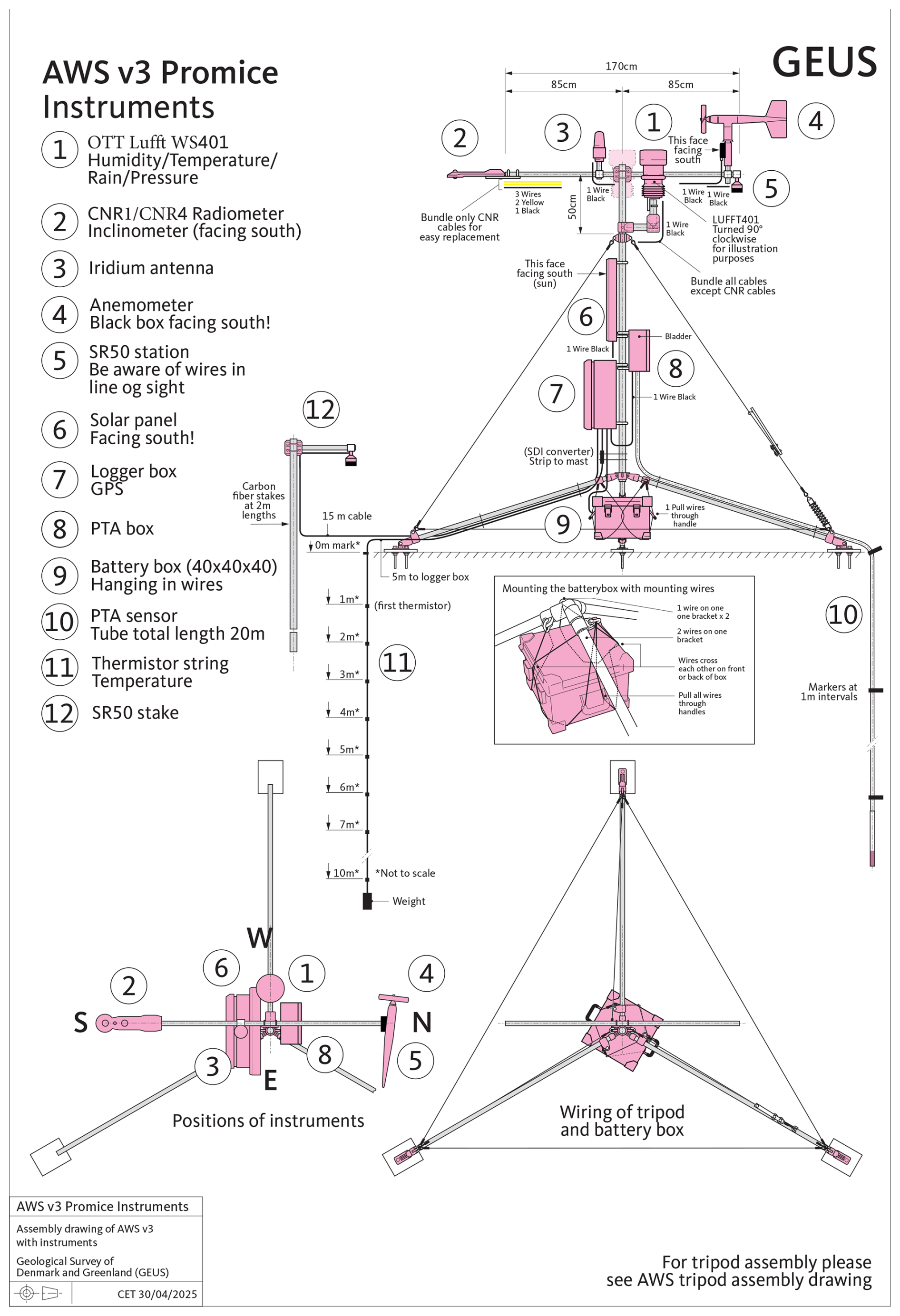
The AWS tripod is constructed using 32 mm (1.25 in.) and 44 mm (1.75 in.) diameter aluminum tubes, reinforced with 3 mm braided stainless-steel wires to form a stable tetrahedral structure (Figs. 4 and 5). Most sensors are mounted on a 1.7 m long horizontal boom positioned 2.7 m above the surface (Fig. 4). To enhance stability, a battery box weighing approximately 50 kg is suspended beneath the mast on wire ropes with shackles, lowering the centre of gravity of the AWS installation. The tripod design allows it to be folded for transport in small helicopters and tilted for sensor replacements.

The sensor housing with thermometer and hygrometer is located approximately 2.6 m above the ice surface (i.e. as high as possible underneath the sensor boom). The measurement height varies when a winter snow cover is present (Fig. 4, item 1). The inclinometer is mounted on the sensor boom (Fig. 4, item 2) and aligned with the radiometer to allow for tilt correction of the CNR1 shortwave radiation measurements. In contrast to the previous setup described in Fausto et al. (2021), the inclinometer and compass are now integrated into the CNR4 radiometer for improved alignment. The radiometer is installed as an extension of the boom and faces south, as shown in Figs. 4 and 5. In the latest AWS designs, the compass also provides orientation data to record any rotation of the boom or tripod. The wind sensor is mounted on the opposite side of the boom from the radiometer (Fig. 4, item 4), measuring approximately 40 cm above the boom. The sonic ranger is mounted on the boom directly under the wind sensor with a distance to the ice surface of approximately 2.6 m (Fig. 4, item 5), while the SR50A mounted on a stake is drilled into the ice and melts out with the ablating ice surface during summer (Fig. 4, item 12). As the tripod rests freely on the ice surface, it moves down as the ice melts, meaning the sonic ranger measurements on the AWS do not capture ice melt, only snowfall and snowmelt. The separate sonic ranger on the stake (8 m), constructed from 40 mm carbon fibre tubing and typically drilled 6–7 m into the ice, does record any sort of accumulation and ablation (Fig. 4). In addition to sensor-related uncertainties, occasional complications arise when a stake assembly melts out and falls over. The data logger enclosure also includes the Iridium modem and GPS receiver. A single-frequency GPS receiver is used to measure the position and elevation of each station to determine e.g. ice flow velocity (Fig. 4, item 7). The Iridium antenna is mounted on the boom (Fig. 4, item 3) to ensure optimal satellite reception. The PTA bladder box (Fig. 4, items 8 and 10) is mounted on the mast approximately 1.5 m above the ice surface, with any spare or melted-out hose resting on the surface and the remaining hose drilled into the ice, measuring ice melt. Figure 4 illustrates the free-standing AWS tripod, which moves downward as the ice surface ablates, while the hose itself melts out of the ice. This process reduces the hydrostatic pressure exerted by the liquid column over the transducer, allowing direct calculation of ice ablation. The power system includes rechargeable batteries connected to a relatively small solar panel without a charge controller (Fig. 4, items 6 and 9). The solar panel is mounted on the mast, facing south, and positioned well above the ice surface to prevent winter snow accumulation from covering the panel. The thermistor string (Fig. 4, item 11) is drilled 10 m into the ice.

All stations on bedrock uses the tripod setup without a pressure transducer assembly, a thermistor string, and a stake assembly. AWS KAN_B additionally includes a rain gauge of type Geonor T200B for precipitation measurement. KAN_B is the only station equipped with a Geonor T200B, whose rain-gauge setup differs from the other stations and is not part of the standard configuration.

Table 3 The table lists the core site metadata for each AWS, including Site ID, the individual stations composing each site, and their geographic position (latitude and longitude in WGS84). It also specifies the local setting (location type), overall station configuration (site type), and the original installation date. Together, these fields provide essential context for interpreting the dataset and understanding the structural layout of the AWS network.

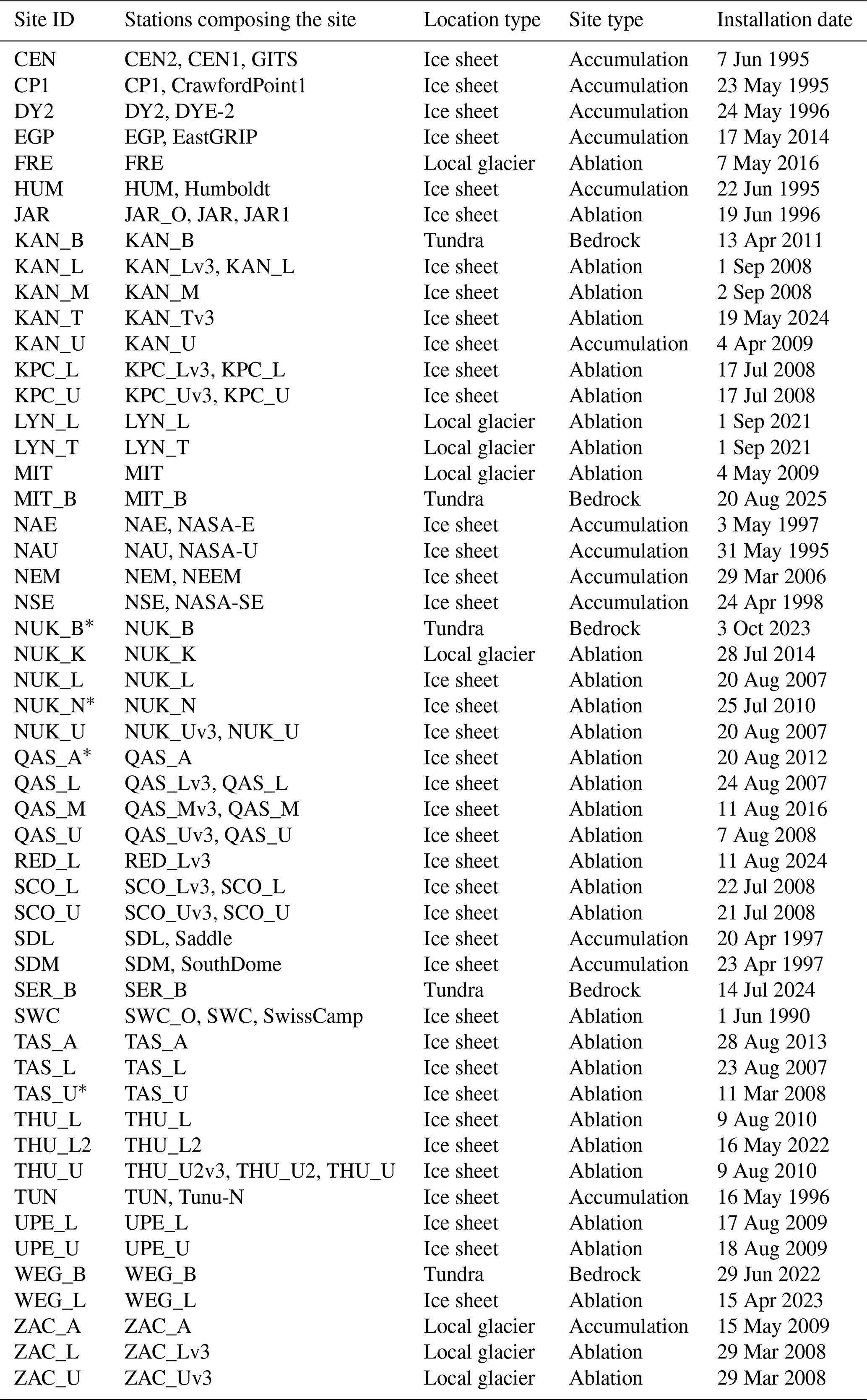
^∗ Discontinued sites.

2.3 Site-Specific Merging of Data from Multiple Stations

We distinguish between “station” and “site”, where station is one specific AWS and site is a location that may encompass data from more than one AWS (Table 3). The difference between station and site is as follows:

• The term “station” refers to a coherent AWS installation. A given station can sometimes be upgraded (instruments, datalogger, etc.) or relocated. Vandecrux et al. (2023) define GC-NET AWS data collected before the GEUS takeover as “historical data”, which they revisited by removing errors and applying quality adjustments to meet higher standards. This effort ensured compatibility between historical records and data from present-day accumulation-area stations. New ablation-area tripod stations, initially labeled “v3” to replace decommissioned “v2” models, have been installed at most sites. As a result, multiple stations at a given site can now be consolidated into a single site-specific dataset.

• The term “sites” refers to locations with a radius of less than 4 km where one or more stations are, or have been, operational. For simplicity, each site is named and recorded as site_id in the data file attributes. For example, the site QAS_U includes data from both the QAS_U and QAS_Uv3 stations, while the site SDM includes data from the historical South Dome station and the current SDM station. Nearby stations can be active simultaneously, producing redundant observations at a given site. The complete list of sites is provided in Table 3 and see Fig. 1 for examples.

In the updated, PROMICE | GC-Net data product, the distributed files are site-specific. The list of the 52 sites and the names of distinct stations that are currently grouped under each site appears in Table 3.

2.4 Measurements and data transmissions

Measurements are taken every 10 min and stored in the data logger. For most measured variables, the logger converts voltage readings into physical values using simple scaling relations based on calibration coefficients specific to each instrument. In cases where identical sensors may have different calibration coefficients, such as the radiometer and pressure transducer, voltage is converted using automatic procedures (to be described in section 3). This approach allows sensor replacements without requiring changes to the logger program.

The AWSs transmit hourly averages based on measurements occurring every ten minutes year round. Older AWS versions (Fausto et al., 2021) transmit hourly averages between day of the year 100 and 300 (10 April and 26 October in non-leap years). Parameters that do not have significant sub-daily changes (GPS position, station tilt, surface height, etc.) are transmitted less frequently (every 6 h) to reduce the transmission cost. In winter, between day of the year 300 and 100, the previous AWS versions transmitted daily averages of all parameters to limit power consumption by the satellite modem when little solar charging was available. Transmission is done through the Iridium satellite network that has coverage even at the northernmost latitudes. The Iridium Short Burst Data service transmits up to 340 bytes per message. The logger program ensures successful data transmission by implementing a message queue to handle situations where the Iridium satellites are unavailable. This relatively low-power operation mode ensures unnecessary transmission attempts with a low rate of message loss. Moreover, the logger program encodes the data in a binary format before transmission, which reduces the size of the message, thereby reducing transmission costs by about two-thirds.

2.5 AWS maintenance

To ensure reliable and accurate measurements, instruments in the field are replaced according to a maintenance schedule informed by manufacturer recommendations and operational experience, such as battery life and performance when charging without a charge regulator. This schedule serves as a guideline, but field crews cannot always return to an AWS in time to perform a scheduled sensor swap (Table 2). For instance, the AWSs in northeastern Greenland (KPC; Fig. 1) are visited only every 3–4 years due to their remote location. Fortunately, these remote AWSs experience less melt, lower accumulation, and less severe storms compared to several other regions, so that some aspects of the maintenance visits become less urgent.

Maintenance visits at ablation sites (tripod type on ice) are typically performed by two people and last 2–4 h, carrying out data download from the logger, documenting the state of the AWS, replacing sensors scheduled for recalibration, re-drilling the PTA, thermistor string and sonic ranger stake in ice, and conducting any necessary repairs.

Maintenance visits at accumulation sites (mast type in snow/firn) are typically performed by a core team of four people, last 3–7 h, and often involves assistance from further personnel, e.g., helicopter or aircraft crew. Apart from data download and instrument replacement, maintenance visits at accumulation sites include:

• Extending the mast to counter snow accumulation.

• Digging out and raising the battery box.

• Retrieving a snow pit density and snow temperature profile at 10 cm vertical resolution, covering the snow accumulated since the last visit.

• Drilling a 10 m firn core for density profiling at core breaks and stratigraphic characterization.

• Measuring and repositioning a snow stake fitted with a board to mark the time of maintenance visit.

• Performing a GNSS survey of the mast position and elevation.

For the thermistor string, the cable (including the cap) connecting the thermistor system with the AWS is detached and replaced (it is buried deep in snow) and an additional 2 m polypropylene pipe is added, while the entire thermistor string is carefully pulled up to reposition the top thermistor at the surface level.

Further measurements at accumulation sites have included radar surveys of snow depth and snow micro-penetrometer measurements (Schneebeli et al., 1999). The aim is to visit all the accumulation sites annually, but occasionally, AWS's in low-accumulation areas are visited biannually, unless instruments require maintenance or replacement.

3 Data product

This section details the data processing pipeline, including filtering, measurement corrections, and the derivation of variables, as well as the computation of hourly, daily, and monthly averages. The following sections also describe the AWS dataset contents, variable definitions, data types, and key differences in processing for ablation- and accumulation-area stations. Together, these sections present the new and updated AWS dataset.

3.1 Data Processing Pipeline

Here, we use the data procesing pipeline called “pypromice”. pypromice is the open-source Python library used for processing raw AWS data in Greenland (How et al., 2023a, b). It provides tools for importing, cleaning, and quality-controlling raw AWS measurements, computing derived meteorological variables such as surface temperature, and performing temporal aggregation and visualization. pypromice enables researchers to efficiently work with large AWS datasets, reproduce analyses, and integrate AWS observations with other datasets.

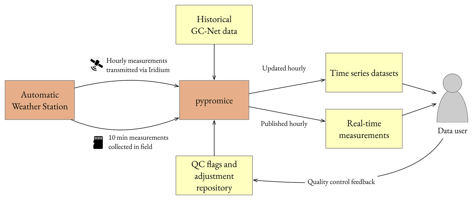
Figure 6 Operational components and key data inputs of the PROMICE processing pipeline. The workflow integrates AWS measurements, historical GC-Net records, and quality-control adjustments performed in pypromice to generate hourly updated time series and real-time data products. Brown boxes represent processing components, while yellow boxes denote data entities, including both input datasets and final outputs.

The processing pipeline is structured around two operational components and two key data inputs (Fig. 6):

• Active AWS deployments: Each AWS logs 10 min data locally and transmits hourly measurements via Iridium. The complete set of 10 min data files are retrieved and ingested into the pipeline after maintenance visits.

• pypromice: This is the central processing component responsible for fetching, processing, and publishing data from all active AWS; documented in How et al. (2023b).

• QC flags and adjustments repository: Manual quality control is managed via the public GitHub repository “PROMICE-AWS-data-issues”, serving as a collaborative space for data review and external feedback.

• Historical GC-Net dataset: A pre-processed dataset containing historical data from the GC-Net network (Vandecrux et al., 2023) is used as an additional data input to obtain long-term time series for sites.

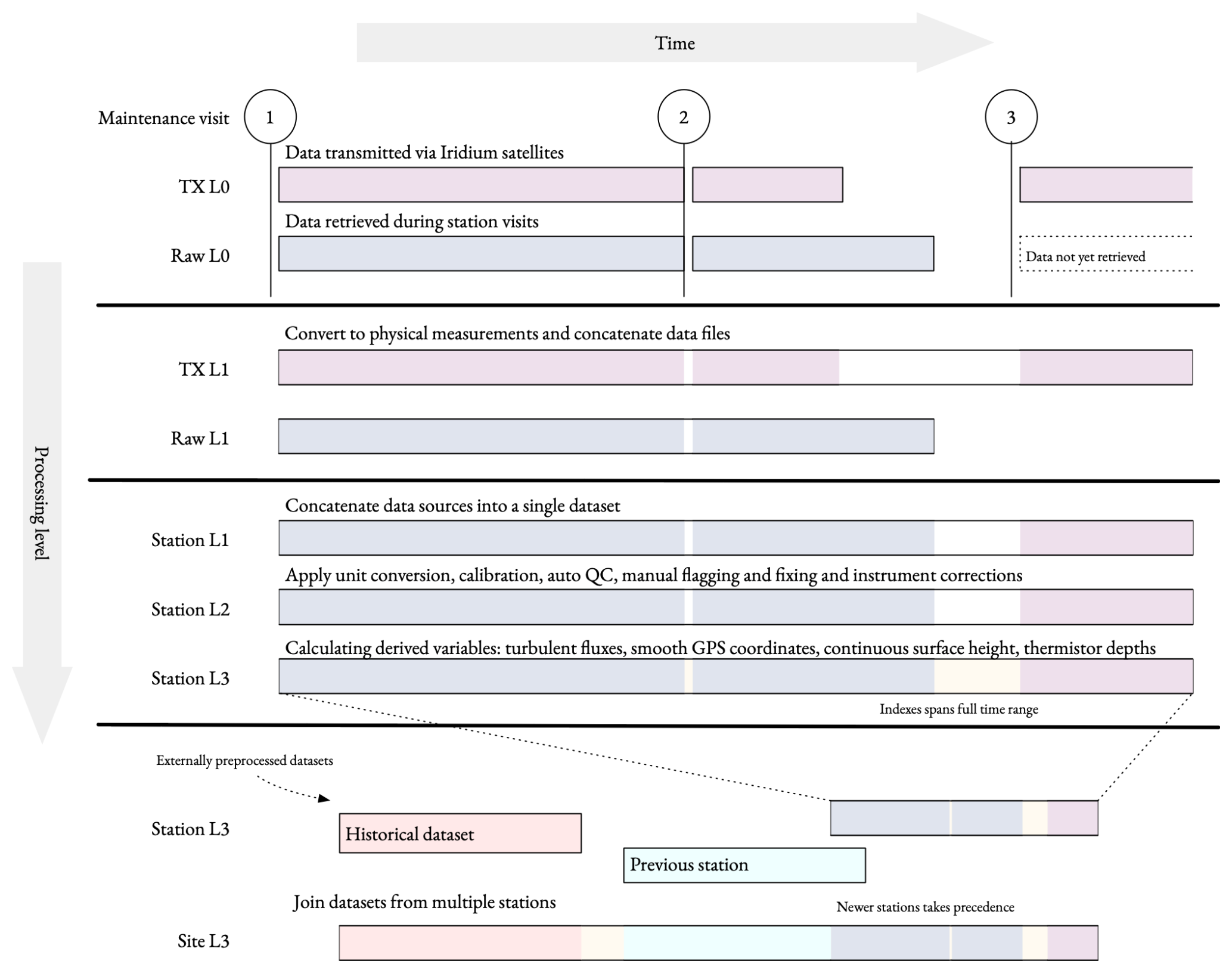
Figure 7 Illustration of the AWS data processing pipeline from raw L0 chunks to final L3 site-specific products. The horizontal axis shows measurement time; the vertical axis shows processing level. Station-specific L1–L3 series are generated from L0 data and merged with historical and previous-station datasets (bottom) to produce continuous site-level time series. Colors indicate the origin of data in the final product: blue represents high-resolution raw data retrieved during maintenance visits, while red denotes data acquired through transmissions. Orange and cyan indicate additional external or supplementary data sources contributing to the time series. Light yellow marks periods without available data (gaps). White areas denote intervals where no data are present in the processing chain.

The AWS data pipeline organizes the dataset into four hierarchical processing levels (Fig. 7). Each level represents a distinct stage in the transformation and validation of the data, from raw logger output to finalised quality-controlled datasets with a selection of transformed and derived variables.

• Level 0 (L0): Holds the raw data as recorded by the station data loggers. These measurements are collected either via Iridium transmissions or during field visits and remain uncalibrated. As logger configurations vary between stations, so do the formats, variables, and sampling frequencies. Level 0 serves as an immutable source layer from which all further processing is derived.

• Level 1 (L1): Converts raw measurements into physically meaningful units and standardizes the dataset across stations. This involves applying calibrations, decoding sensor outputs, and adopting a consistent variable naming scheme, resulting in a unified and interpretable data structure.

• Level 2 (L2): Adds quality control and initial physical interpretation. It incorporates both manual corrections and automated checks, applies filters to remove or correct suspect values, and computes selected derived variables such as cloud cover, albedo, and corrected radiation measurements.

• Level 3 (L3): Synthesizes the processed data into a set of derived variables suitable for research applications. This includes turbulent heat fluxes, continuous surface and snow height records, time-dependent station positions, and other higher-level outputs required for e.g., energy and surface mass balance studies.

In addition to the processing levels, the pipeline defines a set of core concepts for modelling time and space. A station refers to a specific version of an AWS for a specific location, covering both tripod and mast stations. The configuration and instruments of the station can change over time due to maintenance visits. Periods with a fixed setup are treated as individual L0 data files, ensuring consistency with related parameters such as calibration coefficients. A site is an area that may include multiple stations. As described in Sect. 2.3, station data can be aggregated into sites to produce longer time series.

3.1.1 Data Acquisition

There are multiple types of L0 data collected from the AWS data loggers, while the formats can vary depending on local installations and logger programs.

• Raw data: Recorded every 10 min and retrieved from the data logger during maintenance visits. This can either be retrieved directly from the memory card or downloaded from the data logger.

• SlimTable: A format used by older AWS as a lighter hourly aggregated raw format due to limited logger memory.

• Transmission data: Collected on an hourly basis and includes a subset of the variables from the latest record.

The pipeline supports all formats with raw data, when available, in favour of transmissions. Transmissions cover the period since the latest visit and serve as a fallback in case of missing or corrupted raw data. New transmission data is processed in near-real-time every hour, with a latency of approximately five minutes between transmission and production-ready data.

3.1.2 pypromice

AWS data are processed by the pypromice Python package (https://github.com/GEUS-Glaciology-and-Climate/pypromice, last access: 28 May 2026) (version 1.5.1), a peer-reviewed suite of algorithms in a standardised workflow for transforming original AWS data (hereafter referred to as L0) to a processed, finalised, user-ready L3 data product (How et al., 2023a) (Fig. 7). The pypromice package is available via pypi and conda-forge for easy deployment and contains full-coverage unit testing to ensure continuous integration and compatibility across versions and updates. Pypi is the official repository for Python packages, while conda-forge is a community-maintained channel that provides conda-compatible packages across platforms.

3.1.3 Dataset Variables: Derived and Corrected Variables

This section provides an overview of the derived and corrected variables included in the dataset. It outlines the calculations used to generate these variables and presents them in a structured dataset variables table. Methods for deriving new variables or correcting existing ones are described, ensuring transparency and reproducibility of the data processing steps. In the available netcdf files, the long variable names and a dedicated attribute indicate whether a variable is a direct measurement or calculated in post-processing. This metadata is also summarized in a CSV file “variable.csv” distributed along with the data (How et al., 2022a).

Specific humidity

The specific humidity q (in kg kg⁻¹) is calculated from the relative humidity RH (with respect to water or ice, depending on the temperature) using the following equations:

$$\begin{array}{}\text{(6)}& q={\displaystyle \frac{\text{RH}}{\mathrm{100}}}\cdot q_{\text{sat}},\end{array}$$

where

$$\begin{array}{}\text{(7)}& q_{\text{sat}}={\displaystyle \frac{\mathit{\epsilon }{e}_{\text{sat}}}{p-(\mathrm{1}-\mathit{\epsilon })e_{\text{sat}}}}.\end{array}$$

In these equations, ε=0.622 is the ratio of the specific gas constants for dry air and water vapor, p is the air pressure (in Pa), and e_sat is the saturation water vapor pressure (in Pa) over either ice (for below freezing) or water (for above freezing), as calculated following Goff and Gratch (1946).

Surface temperature

The surface temperature T_s (in °C) is calculated using Stefan–Boltzmann law by using the measured downward and upward longwave irradiance (LR_in and LR_out, respectively) with the following equation:

$$\begin{array}{}\text{(8)}& T_{\mathrm{s}}={\left({\displaystyle \frac{{\mathrm{LR}}_{\mathrm{out}}-(\mathrm{1}-\mathit{\epsilon }){\mathrm{LR}}_{\mathrm{in}}}{\mathit{\epsilon }\cdot \mathrm{5.67}\times {\mathrm{10}}^{-\mathrm{8}}}}\right)}^{\mathrm{0.25}}-T_{\mathrm{0}},\end{array}$$

where the ice sheet surface emissivity is assumed to be ε=0.97 and T₀ = 273.15 K.

Turbulent energy fluxes

With key surface meteorological values known, such as temperature from longwave radiation, saturated humidity, and zero wind, turbulent heat flux gradients can be calculated without a second sensor boom. The sensible heat flux (SHF) and latent heat flux (LHF), expressed in (W m⁻²), are estimated from vertical gradients in wind speed, potential temperature, and specific humidity between the instrumented boom height and the surface, following the method described by Van As et al. (2005) and Van As (2011). Based on Monin–Obukhov similarity theory, SHF and LHF are approximated as:

$$\begin{array}{}\text{(9)}& {\displaystyle }& {\displaystyle }\text{SHF}=\mathit{\rho }{C}_{\mathrm{p}}{\mathit{\kappa }}^{\mathrm{2}}{\displaystyle \frac{u}{\ln \frac{z_{\mathrm{u}}}{z_{\mathrm{0}}}-{\mathit{\psi }}_u}}{\displaystyle \frac{T-T_{\mathrm{s}}}{\ln \frac{z_{\mathrm{T}}}{z_{\mathrm{0},\mathrm{T}}}-{\mathit{\psi }}_T}},\text{(10)}& {\displaystyle }& {\displaystyle }\text{LHF}=\mathit{\rho }{L}_{\mathrm{s}/\mathrm{v}}{\mathit{\kappa }}^{\mathrm{2}}{\displaystyle \frac{u}{\ln \frac{z_{\mathrm{u}}}{z_{\mathrm{0}}}-{\mathit{\psi }}_u}}{\displaystyle \frac{q-q_{\mathrm{s}}}{\ln \frac{z_{\mathrm{q}}}{z_{\mathrm{0},\mathrm{q}}}-{\mathit{\psi }}_q}},\end{array}$$

where ρ denotes the air density, and C_p = 1005 $\mathrm{J}{\mathrm{K}}^{-\mathrm{1}}{\mathrm{kg}}^{-\mathrm{1}}$ is the specific heat capacity of air at constant pressure. The latent heat of sublimation and evaporation are L_s = 2.83 × 10⁶ J kg⁻¹ and L_v = 2.50 × 10⁶ J kg⁻¹, respectively. The von Kármán constant is κ=0.4. Positive fluxes contribute energy to the surface, whereas negative fluxes withdraw energy from it.

To estimate turbulent heat fluxes, we require measurements of the following variables at given heights: wind speed (z_u), temperature (z_T), and specific humidity (z_q). Additionally, we need the surface roughness lengths for momentum (z₀), heat (z_0,T), and moisture (z_0,q). A constant value of z₀ = 0.001 m is used, while $z_{\mathrm{0},\mathrm{T}}=z_{\mathrm{0},\mathrm{q}}$ is calculated based on the formulation for rough surfaces by Smeets and Van den Broeke (2008a, b). Atmospheric stability corrections are applied using the functions ${\mathit{\psi }}_{\mathrm{u},\mathrm{T},\mathrm{q}}$ from Holtslag and De Bruin (1988) for stable conditions and from Paulson (1970) for unstable conditions. Surface temperature (T_s) is derived from longwave radiation (see Eq. 8), and the surface specific humidity is assumed to be at saturation, i.e., q_s=q_sat.

Several sources of uncertainty affect the calculation of sensible (SHF) and latent heat fluxes (LHF). The aerodynamic surface roughness length z₀ varies with surface type (Brock et al., 2006) and over time (Smeets and Van den Broeke, 2008a, b). Assuming a constant value of z₀ = 0.001 m may overestimate surface roughness in snowy conditions and thus lead to overestimations of both turbulent fluxes.

Box and Steffen (2001) showed that one- and two-level methods underestimate downward latent heat flux under extreme stability. Miller et al. (2017) found similar biases in sensible heat flux, with one-level methods offering longer records. Fausto et al. (2016a, b) highlighted the use of unrealistically high surface roughness lengths (z₀) to match surface energy balance closure with melt-driven ablation rates during intense heat flux events. Turbulent heat flux estimates over ice and snow are uncertain due to assumptions of surface homogeneity, stable polar boundary layers limiting turbulence, surface variability, scarce measurements, and sensitivity to temperature errors. Thus, these estimates require cautious interpretation.

Tilt correction of downward shortwave radiation

Tilt correction of solar radiation follows the method outlined by Van As (2011), which is also described by Fausto et al. (2021). Downward shortwave radiation (SR_in) is composed of both diffuse and direct beam components, but only the direct beam component requires correction for surface tilt. For a horizontal radiation sensor, the direct beam component, equivalent to SR_in, is reduced by the diffuse fraction (f_dif). For a tilted sensor, SR_in is derived from the measured radiation (SR_in, m) using a correction factor C, as follows:

$$\begin{array}{}\text{(11)}& {\mathrm{SR}}_{\mathrm{in},\mathrm{cor}}={\mathrm{SR}}_{\mathrm{in},\mathrm{m}}{\displaystyle \frac{C}{\mathrm{1}-f_{\text{dif}}+C{f}_{\text{dif}}}},\end{array}$$

with

$$\begin{array}{}\text{(12)}& \begin{array}{rl}C=& \cos \left(\text{SZA}\right)\cdot \left(\sin \right(d\left)\sin \right(\text{lat}\left)\cos \right({\mathit{\varphi }}_{\text{sensor}})\\ & -\sin \left(d\right)\cos \left(\text{lat}\right)\sin \left({\mathit{\theta }}_{\text{sensor}}\right)\cos \left({\mathit{\varphi }}_{\text{sensor}}\right)\\ & +\cos \left(d\right)\cos \left(\text{lat}\right)\cos \left({\mathit{\theta }}_{\text{sensor}}\right)\cos \left(w\right)\\ & +\cos \left(d\right)\sin \left(\text{lat}\right)\sin \left({\mathit{\theta }}_{\text{sensor}}\right)\cos \left({\mathit{\varphi }}_{\text{sensor}}\right)\cos \left(w\right)\\ & +\cos \left(d\right)\sin \left(\right({\mathit{\theta }}_{\text{sensor}}\left)\sin \right({\mathit{\varphi }}_{\text{sensor}}\left)\sin \right(w){)}^{-\mathrm{1}},\end{array}\end{array}$$

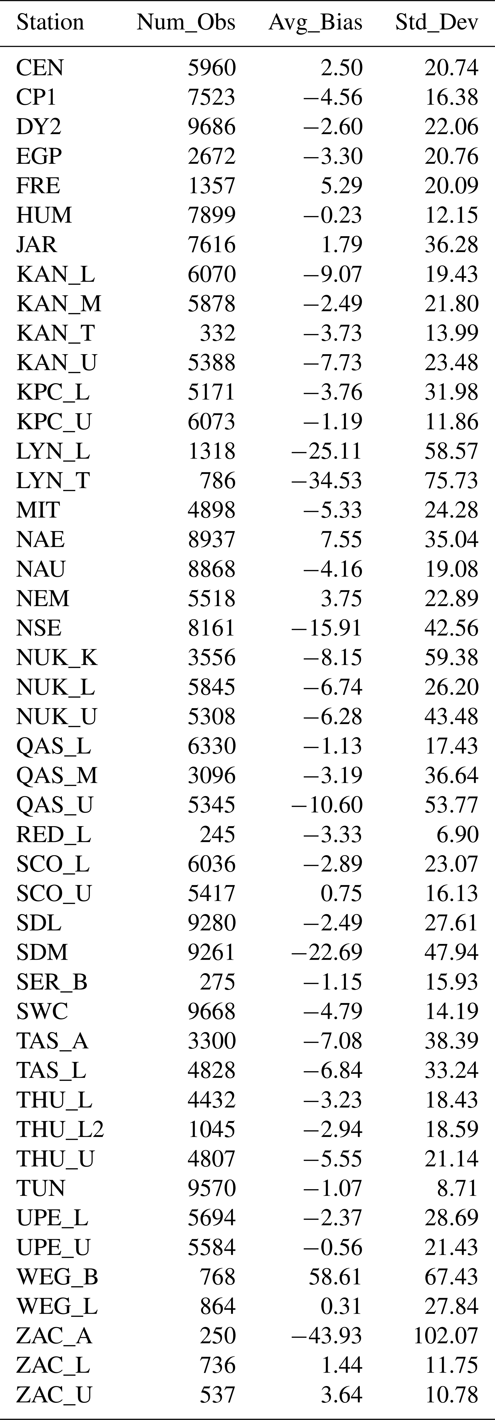
where SZA is the solar zenith angle, d is the solar declination (the angle between the Sun and the Earth's equatorial plane), ω is the hour angle (the angular distance between the Sun's current position and solar noon), lat is the site's latitude in radians, and θ_sensor and ϕ_sensor represent the radiometer's tilt angle and azimuth orientation, respectively. The procedures for calculating d (solar declination), ω (hour angle), and SZA (solar zenith angle) are found in Fausto et al. (2021). Table 4 presents the average bias or correction applied to incoming solar radiation based on Eq. (11). For most AWS stations, the standard deviation shows that the average correction is small, typically less than 15 W m⁻², although a few stations exhibit a broader range of correction values. We estimate the diffuse fraction (f_dif) to range from 0.2 under clear-sky conditions to 1.0 during overcast skies, assuming a linear relationship with cloud cover fraction, as described by Harrison et al. (2008).

Table 4 The table lists, for each station/site, the total number of available downward shortwave-radiation observations (Num_Obs), together with the average difference (Avg_Bias) between the corrected and uncorrected values. The Std_Dev column quantifies the spread of this bias, indicating how consistently the correction affects the measurements across the full time series. Stations with insufficient data coverage are not included in the table.

Cloud cover

To approximate the cloud cover fraction, we rely on the relationship between near-surface air temperature (T_air) and downward longwave radiation (LR_in), following Van As et al. (2005). Specifically, we compute the theoretical clear-sky downward longwave radiation flux using the formula proposed by Swinbank (1963):

$$\begin{array}{}\text{(13)}& {\mathrm{LR}}_{\mathrm{clear}}=\mathrm{5.31}\times {\mathrm{10}}^{-\mathrm{14}}\cdot (T_{\text{air}}+T_{\mathrm{0}}{)}^{\mathrm{6}},\end{array}$$

where LR_clear is the clear-sky longwave radiation flux (in W m⁻²) and T_air is the near-surface air temperature (in Kelvin). This allows us to estimate the cloud cover fraction by comparing observed longwave radiation to the clear-sky baseline.

Theoretical downward longwave radiation under overcast conditions is estimated by assuming black-body emission from a cloud base at the near-surface air temperature. This is calculated using the Stefan–Boltzmann law:

$$\begin{array}{}\text{(14)}& {\mathrm{LR}}_{\mathrm{overcast}}=\mathrm{5.67}\times {\mathrm{10}}^{-\mathrm{8}}\cdot (T_{\text{air}}+T_{\mathrm{0}}{)}^{\mathrm{4}},\end{array}$$

where LR_overcast is the overcast longwave radiation flux (in W m⁻²), T_air is the near-surface air temperature (in °C), and T₀ is the conversion offset to Kelvin (273.15 K).

The cloud cover fraction (cc), constrained within the range [0,1], is then estimated by linearly scaling the observed longwave radiation between clear-sky and overcast conditions:

$$\begin{array}{}\text{(15)}& \mathrm{cc}={\displaystyle \frac{{\mathrm{LR}}_{\mathrm{in}}-{\mathrm{LR}}_{\mathrm{clear}}}{{\mathrm{LR}}_{\mathrm{overcast}}-{\mathrm{LR}}_{\mathrm{clear}}}}={\displaystyle \frac{f_{\text{dif}}-\mathrm{0.2}}{\mathrm{0.8}}}.\end{array}$$

The cloud cover estimation is only valid over ice and snow surfaces, and therefore is not computed for stations installed on bedrock.

Albedo

Surface broadband solar reflectivity in the 0.3–2.5 µm wavelength range, commonly referred to as albedo (unitless), is derived from 10 min tilt-corrected measurements of downward and upward solar irradiance. Hourly albedo values are computed when the solar zenith angle is under 70° (i.e., when the sun is more than 20° above the horizon), ensuring optimal measurement reliability for the pyranometer. Daily mean albedo values are then calculated from the valid hourly data. Shadows cast by AWS components, such as the mast or sensor arms, together with surface contrast with AWS infrastructure (e.g., solar panel, battery box, legs, enclosure), and the presence of features such as melt ponds beneath the station can reduce observed albedo values by up to 0.03 on average, depending on surface type and snow surface height (Kokhanovsky et al., 2020). This bias source is variable with snow surface height, effectively zero when snow thickness exceeds 1.5 m. Ryan et al. (2017) compared ablation area AWS albedo measurements with unmanned aerial vehicle (UAV)-derived and satellite-based albedo products, finding increasing discrepancies during the late melt season due to spatial inhomogeneity and limited representativeness of point measurements. While Van den Broeke et al. (2004) reported a 5 % uncertainty for pyranometer-based albedo measurements, the instrument manufacturer (Kipp & Zonen) suggests a more conservative estimate of 10 %, adopted here for the calculated albedo values.

Ice surface height

The pressure transducer assembly (PTA; Fig. 4) is sensitive to fluctuations in atmospheric pressure, which can influence the measured signal H_M. To correct for this effect, the contribution of air pressure is removed using the following expression:

$$\begin{array}{}\text{(16)}& H_{\mathrm{L}}=H_{\mathrm{M}}+{\displaystyle \frac{P_{\mathrm{C}}-P_{\mathrm{A}}}{g{\mathit{\rho }}_{\mathrm{l}}}},\end{array}$$

where P_A (in hPa) represents the ambient air pressure, while P_C (in hPa) is the reference pressure specified by the manufacturer during sensor calibration. The gravitational acceleration is assumed to be g = 9.82 m s⁻², and the density of the antifreeze mixture used in the system is ρ_l = 1090 kg m⁻³, for a temperature of 0^∘C. Cumulative variations in the corrected liquid level H_L directly correspond to ice surface ablation. Fausto et al. (2012, 2016a) validated PTA-derived ablation measurements against manual hose-based readings and sonic ranger data, and found the PTA measurements to be accurate within ± 0.04 m.

Liquid precipitation correction

Following Box et al. (2023), we correct liquid precipitation measurements for undercatch using wind speed (U). We apply the undercatch correction factor (k) for an unshielded Hellmann-type gauge under liquid-only precipitation conditions, using the catch-efficiency relation from Yang et al. (1999):

$$\begin{array}{}\text{(17)}& k={\displaystyle \frac{\mathrm{100}}{\mathrm{100}-\mathrm{4.37}U+\mathrm{0.35}{U}^{\mathrm{2}}}},\end{array}$$

where U is wind speed (in m s⁻¹) at measurement height. Yang et al. (1999) derived a well-tested wind-based correction for unshielded Hellmann-type gauges using extensive World Meteorological Organization intercomparison data, showing that wind speed is the primary driver of undercatch. Because our gauge type matches theirs, and the method performs robustly across varied climates, their relationship is an appropriate choice. Some uncertainty remains, as wind alone cannot explain all undercatch variability and the correction was originally derived from daily mean wind speeds up to 6.5 m s⁻¹, but is assumed to be applicable to hourly wind speed data. For wind speeds exceeding 6.5 m s⁻¹, an extrapolated correction is applied (Yang et al., 1999). As with all automated precipitation measurements, considerable uncertainty persists in the corrected values, as wind speed alone does not fully account for the observed undercatch.

Moreover, only rainfall is considered in this undercatch correction by excluding measurement periods where air temperature is below −2 °C. However, this does not eliminate the affect of delayed snow melt errors, when snow accumulates in the gauge and is only registered as precipitation as it melts into the tipping bucket. Such instances can occur during short atmospheric warm spells within otherwise sustained below-freezing conditions during winter. As a result, corrected rainfall should be used and interpreted with caution. In addition, no corrections are applied for evaporation, wetting, or trace precipitation.

3.2 Dataset structure

Multiple versions of the AWS datasets are available, reflecting different processing levels, temporal resolutions, and aggregation scales (station vs. site):

• L2: Station data, hourly

• L3: Site data, hourly, daily, and monthly

The L2 datasets are quality-controlled and noise-filtered. This is the least processed public product, closely reflecting the original station measurements. The L3 datasets are the highest level of processed data, including derived variables, and is documented in Sect. 3.2.2. The L3 product is provided only at the site level, enabling the creation of longer, continuous time series.

3.2.1 Metadata and Data Discoverability Attributes

The datasets are distributed with a comprehensive set of metadata, following the Climate and Forecast (CF, Hassell et al., 2017) conventions and the Attribute Convention for Data Discovery (ACDD). In addition, specific attributes are included to capture station- and site-levels details relevant for interpretation, reuse and reproducibility. For example, the specific attribute site_type is added to describe the environment type of the installation site (e.g., ablation, accumulation, or tundra).

Table 5 The table lists all variables included in the Level-3 data products, specifying the variable name, physical units, and a brief description of each parameter. Together, these fields provide users with a clear overview of the available measurements and their intended interpretation within the dataset.

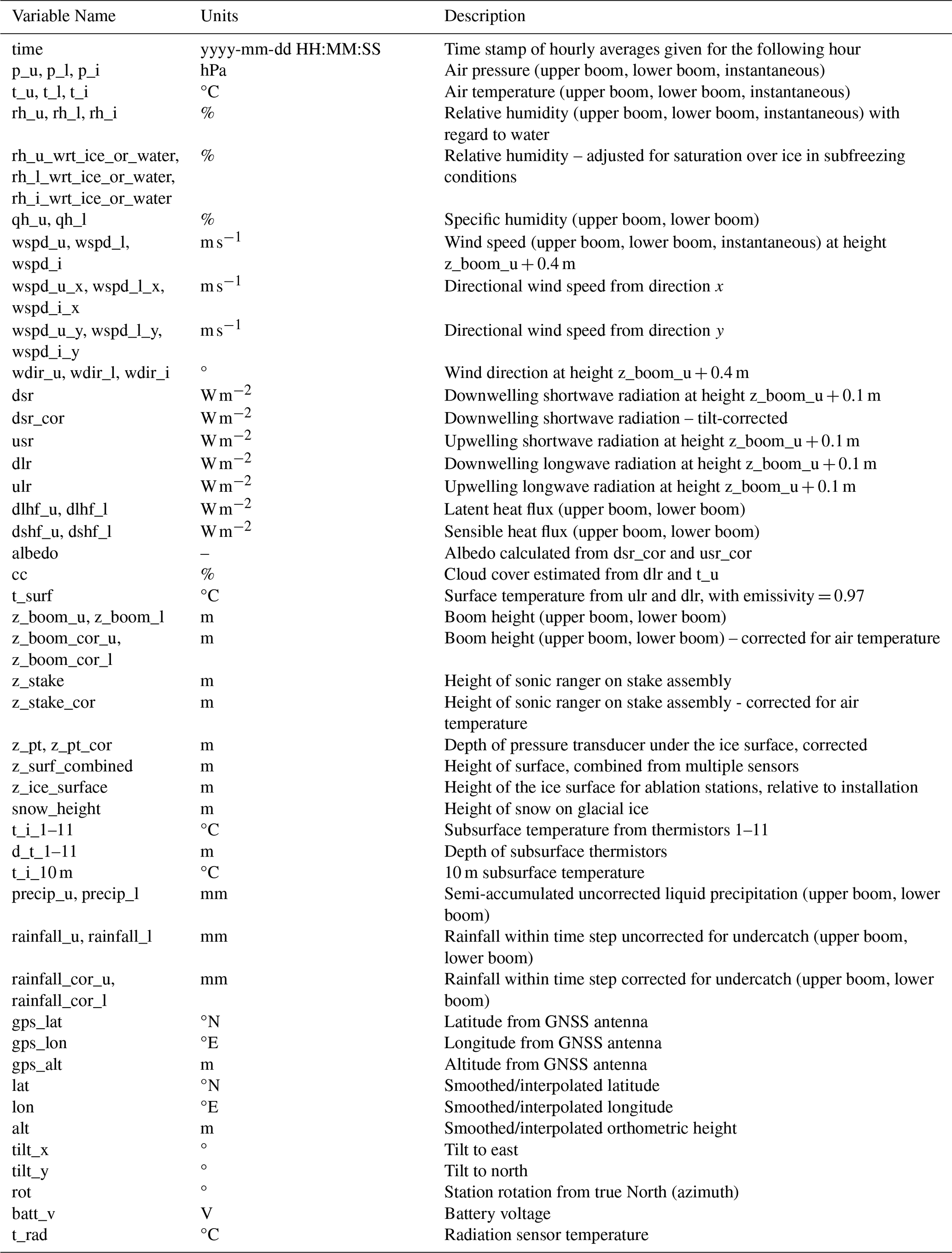
3.2.2 Data variables

The data variables are CF-compliant according to CF-1.7 and use an updated naming convention relative to our earlier products. The L3 hourly datasets contain a full set of data variables from our processing pipeline and are summarised in Table 5. Many variables are measured at both the upper and lower boom in cases where stations or sites follow the accumulation area two-boom station design. In addition, instantaneous measurements are provided for key variables (air temperature, air pressure, relative humidity, wind speed, and wind direction), whereby instantaneous measurements are recorded at the top of each hour. For stations or sites with the ablation area one-boom station design, variables are assigned as upper boom measurements, with no corresponding lower boom values provided.

3.2.3 File formats

The datasets are provided in both NetCDF and CSV formats. The data itself is unchanged between these two versions, however, the NetCDF format includes metadata and variable attributes which better inform about the collection and quality of the data. We therefore recommend users adopt the NetCDF format where possible.

3.3 Quality Control and Filtering Routines

The transformation from L1 to L2 introduces quality control mechanisms. This includes the application of automated filters as well as the integration of manual flags and adjustments maintained in the public repository: https://github.com/GEUS-Glaciology-and-Climate/PROMICE-AWS-data-issues (last access: 12 November 2025).

Four stringent filtering routines are adopted in the production workflow to remove erroneous data and outliers. These filtering routines are performed and included in the L2 dataset (i.e., performed between L1 and L2).

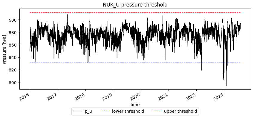
Figure 8 Example of how the threshold filter operates for air pressure. p_u denotes individual air-pressure measurements from the station NUK_U. The thresholds indicate the expected range of normal variability (Table B1); values outside these bounds are flagged as potential outliers.

3.3.1 Physical and sensor specific thresholds

An upper and lower threshold is adopted to filter out erroneous measurements (Table B1). These thresholds are informed by the instrument upper and lower measurement capabilities, commonly documented by the instrument manufacturers (see Appendix). Measurements exceeding these limits are flagged as outliers and removed from subsequent analysis. These thresholds are designed to reflect realistic environmental conditions and are adapted to local site characteristics. Figure 8 illustrates an example of how these thresholds are applied to a time series, highlighting the removal of values that fall outside the accepted range.

3.3.2 Rate of change

The rate of change (ROC) between consecutive measurements is used to detect anomalous values in air temperature, air pressure, relative humidity, and subsurface temperature. Initial testing showed that a fixed ROC threshold is insufficient: a high threshold fails to capture outliers, while a low threshold removes valid observations during periods of naturally high variability.

To address this, we compute both forward and backward ROC for each variable and derive a dynamic threshold based on local variability. For each time step, the 95th percentile of the ROC is calculated within a 1 week rolling window (i.e. ± 3.5 d), separately for forward and backward differences:

$${\mathrm{ROC}}_{\mathrm{95}\mathrm{\%}}^{\mathrm{fwd}}\left(t\right),{\mathrm{ROC}}_{\mathrm{95}\mathrm{\%}}^{\mathrm{bwd}}\left(t\right).$$

These percentiles represent the typical variability at that time, taking into account seasonal and site-specific conditions.

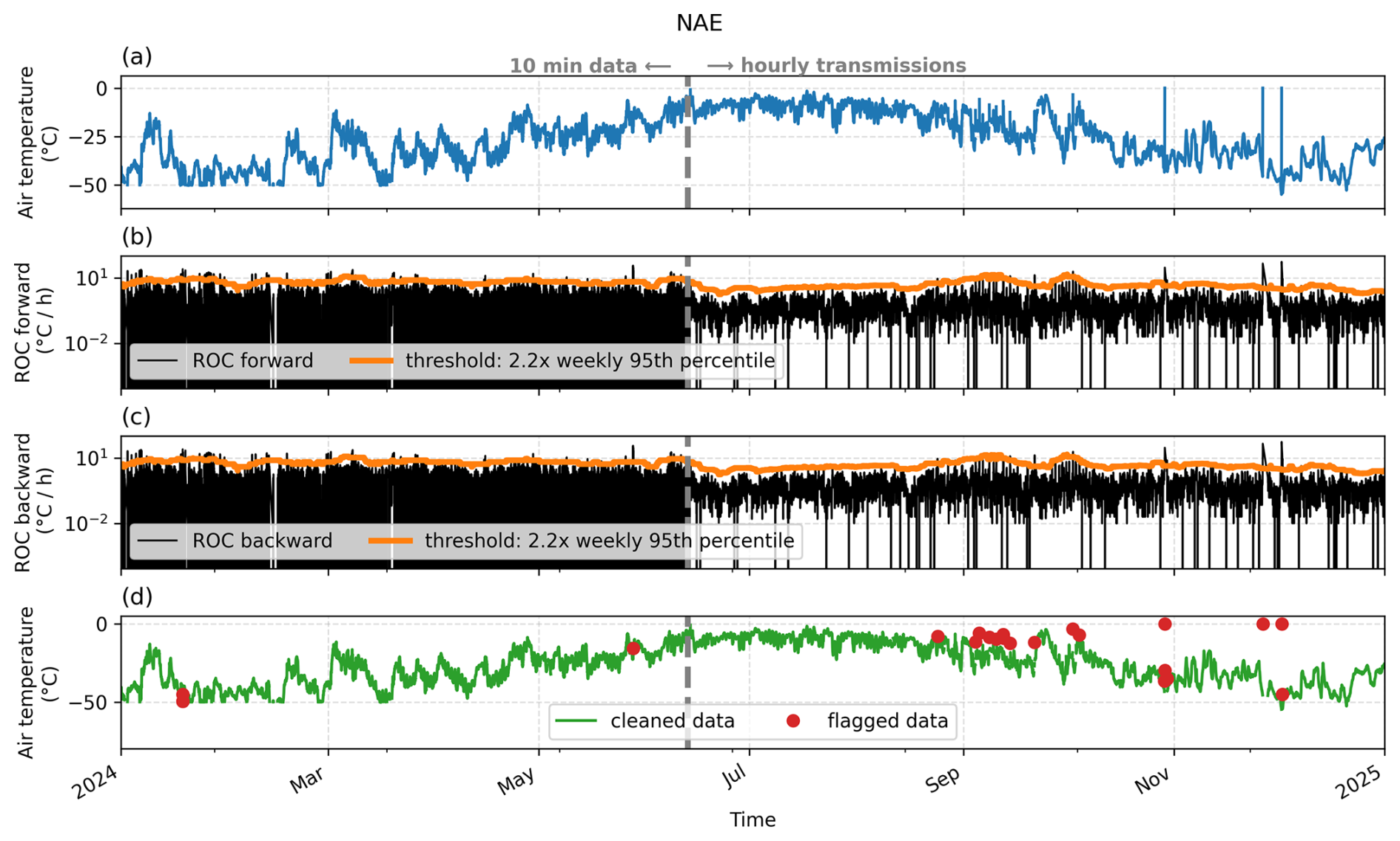
Figure 9 Illustration of the Rate Of Change (ROC) filter on air temperature at the NAE station. (a) Original data. (b) Forward-looking hourly ROC and threshold derived from the 95th percentile of ROC values within ± 3.5 d of each sample and a variable-specific factor (2.2 for air temperature). Note the logarithmic vertical scale. (c) Same as (b) but for backward looking values. (d) Cleaned time series and flagged data. Transition from 10 min data to hourly transmissions is marked with gray dashed lines.

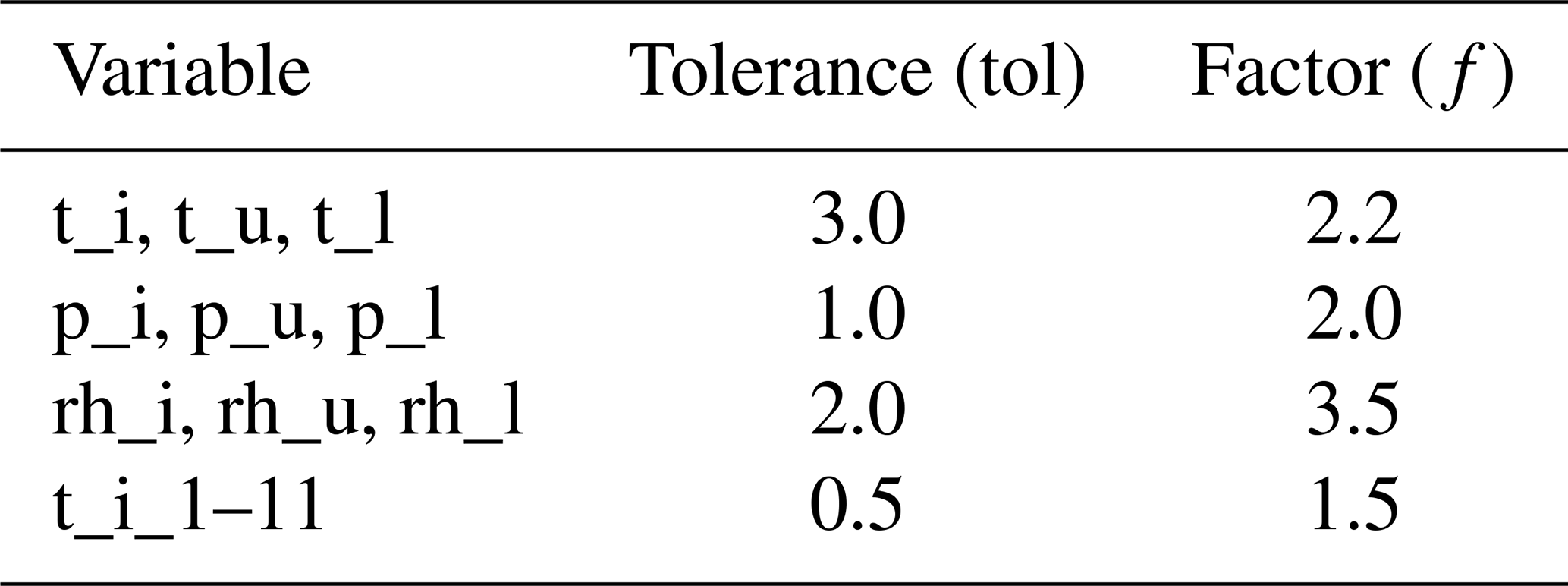
A value is flagged as a potential outlier if both its forward and backward ROC exceed a variable-specific multiple of the corresponding threshold:

$$\begin{array}{rl}{\mathrm{ROC}}^{\mathrm{fwd}}\left(t\right)& >f\cdot {\mathrm{ROC}}_{\mathrm{95}\mathrm{\%}}^{\mathrm{fwd}}\left(t\right)\text{ AND }{\mathrm{ROC}}^{\mathrm{bwd}}\left(t\right)\\ & >f\cdot {\mathrm{ROC}}_{\mathrm{95}\mathrm{\%}}^{\mathrm{bwd}}\left(t\right),\end{array}$$

where ROC^fwd(t) and ROC^bwd(t) denote the forward and backward ROC values at time step t. The factor f is variable-specific, e.g. f=2.2 for air temperature and f=3.5 for relative humidity (Table 6). Figure 9 shows the ROC filter applied to NAE air temperature data. In the first part of the series, the 10 min data appear outlier-free, although forward- and backward-looking ROC values often exceed their thresholds (Fig. 9a–c, left of the gray line). In the second half, the hourly data contain clear outliers and exhibit several threshold crossings (Fig. 9a–c, right of the gray line). Thanks to adaptive thresholding and reassessment of flagged samples via linear interpolation, the ROC filter flags only a few early values while correctly identifying the obvious outliers later in the record (Fig. 9d).

Table 6 Default thresholds used in the rate-of-change (ROC) quality-control filter. Each entry defines a group of PROMICE AWS variables along with the tolerance parameter (tol) and multiplicative factor (f) applied when detecting anomalously rapid changes. The tolerance controls how closely flagged values must match linear interpolation to be rescued, while the factor scales the rolling 95th-percentile ROC, thereby adjusting the sensitivity of the outlier detection. Higher f values result in more conservative filtering, whereas lower values make the filter more aggressive.

When a time step is adjacent to a data gap, the AND condition above is relaxed to an OR, since only one-sided information is available. At the final time step of the time series (e.g. for incoming transmissions), only the forward condition is applied, with thresholds computed from preceding data.

To avoid removing valid rapid variations, all flagged values are re-evaluated using linear interpolation between neighboring valid measurements. If the observed value lies within a variable-specific tolerance of the interpolated estimate, the flag is removed.

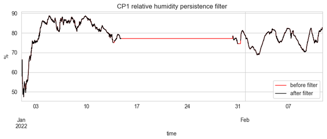
Figure 10 Illustration of how the persistence filter operates. The filter identifies sequences of measurements that remain unrealistically constant over time. Values showing no expected natural variability within a specified window are flagged as potential sensor malfunctions or data artifacts.

3.3.3 Persistence

To detect sensor or data logging malfunctions that result in unchanging measurements, a persistence-based filter is applied as part of the quality control. This filter is designed to identify and flag periods where values remain constant over time, a typical symptom of readout failures or stuck sensors. Persistence filtering targets a known behavior of some logger programs: when a sensor readout fails, the system may fall back to returning the last successfully measured value. If the issue persists, the output becomes artificially constant for hours or days. Figure 10 shows an example of persistent relative humidity readings from station CP1 in January 2022. The red line shows the values before the persistence filter and black line shows after.

3.3.4 Manual filtering and adjustments

At times, manual intervention is required when it is known that the recorded data does not represent the actual conditions at the station. This can occur in situations such as sensor malfunction, the sensor being covered by snow, frost, or rime, or the station becoming tilted or moved during maintenance. Data collected during these periods can either be flagged and removed from the dataset or adjusted using a predefined set of supported operators.

Manual quality control is implemented as an asynchronous and collaborative process based on a public GitHub repository https://github.com/GEUS-Glaciology-and-Climate/PROMICE-AWS-data-issues (last access: 12 November 2025) that allows both internal and external users to contribute by either raising a data issue here, or proposing their own adjustments to the dataset. This is reviewed by a member of the PROMICE | GC-NET AWS data team. Flagging and adjustment rules defined in this repository are integrated into the pypromice production pipeline, where they are applied to the data products on an hourly basis.

3.4 Temporal resolution and success rate

The temporal resolution of AWS data depends on several factors, including the logger program version, data source, measured variable, season, and the operational status of the station. Three primary types of data tables are generated:

• Raw data tables (Raw) contain instantaneous samples with the highest available temporal resolution (10 min), collected during maintenance visits.

• Slim Table Memory (STM) is a compact dataset used in some older CR1000 logger programs. It stores hourly averaged values as an internal backup to maximize storage capacity during long deployments while preserving essential measurements.

• Transmitted data tables (TX) are sent via Iridium including hourly averaged values typically combined with selected instantaneous measurements for real-time use by meteorological offices. Averages are timestamped at the end of each period by the data logger. See Section 3.4 for more information on transmissions.

The processing pipeline is built around hourly averaged measurements, which are standardized to use timestamps at the beginning of each averaging period. In addition, hourly instantaneous values are preserved in separate variables for meteorological analyses, while the higher-frequency raw (10 min) data are primarily used for aggregation and sensor-specific corrections.

Each published AWS dataset is distributed as an hourly sampled time series, which forms the primary product. For user convenience, aggregated daily and monthly datasets are also provided. However, we recommend that users rely on the hourly data when performing further analysis or custom aggregations.

Hourly averages are computed from 10 min values when at least 80 % of the data are available. Daily averages are then derived from hourly averages, also requiring at least 80 % data availability for variables exhibiting clear diurnal variability. For less transient variables, a single measurement is sufficient to compute an average. Finally, monthly averages are calculated from daily averages when at least 80 % of the data are present.

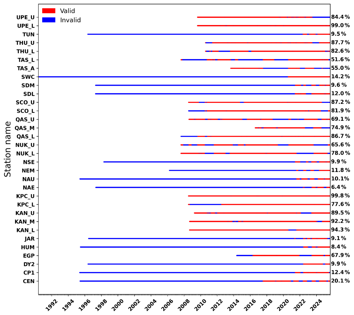
Figure 11 Success rate of the AWS daily data product, expressed as the ratio of days with valid daily averages for all variables required to compute the surface energy budget (air pressure, air temperature, humidity, wind speed, and both shortwave and longwave radiation components). The historical GC-NET dataset does not provide full surface energy balance coverage owing to differing instrumentation at accumulation-area stations. Combined availability of the eight essential variables needed to compute the surface energy balance using daily data products is shown up to the latest data entry on 1 April 2025.

Success rate for key measurements

Using the daily data product, AWS data coverage was assessed using a “success rate”, defined as the ratio of days with valid daily averages for all variables required to estimate the surface energy budget (air pressure, air temperature, humidity, wind speed, and downward and upward shortwave and longwave radiation) to the total days since AWS installation. Performance for these critical variables by site and measurement period is shown in Fig. 11. The historical GC-NET dataset lacks full surface energy balance coverage due to differing instrumentation from all accumulation area stations (Vandecrux et al., 2023).

4 Post-processing

This section outlines the key L2 to L3 post-processing steps applied to the dataset to ensure data consistency, accuracy, and usability. Section 4.1 provides the displacements of AWS, summarized in a dedicated table. Section 4.2 describes the AWS reposition history. Section 4.3 describes methods used to estimate surface height from multiple sensors, supported by illustrations. Section 4.4 covers how thermistor depth is estimated and how 10 m ice or firn temperatures are calculated. Lastly, Sect. 4.5 presents visual examples of representative datasets to illustrate the data product.

Table 7 The table summarizes site-level GPS displacement information, including the station name, the first and latest valid GPS dates, and the resulting observational time span. It also reports the total horizontal displacement and the corresponding elevation change over the measurement period, providing an overview of long-term station movement across the network. Only sites located on ice is included here.

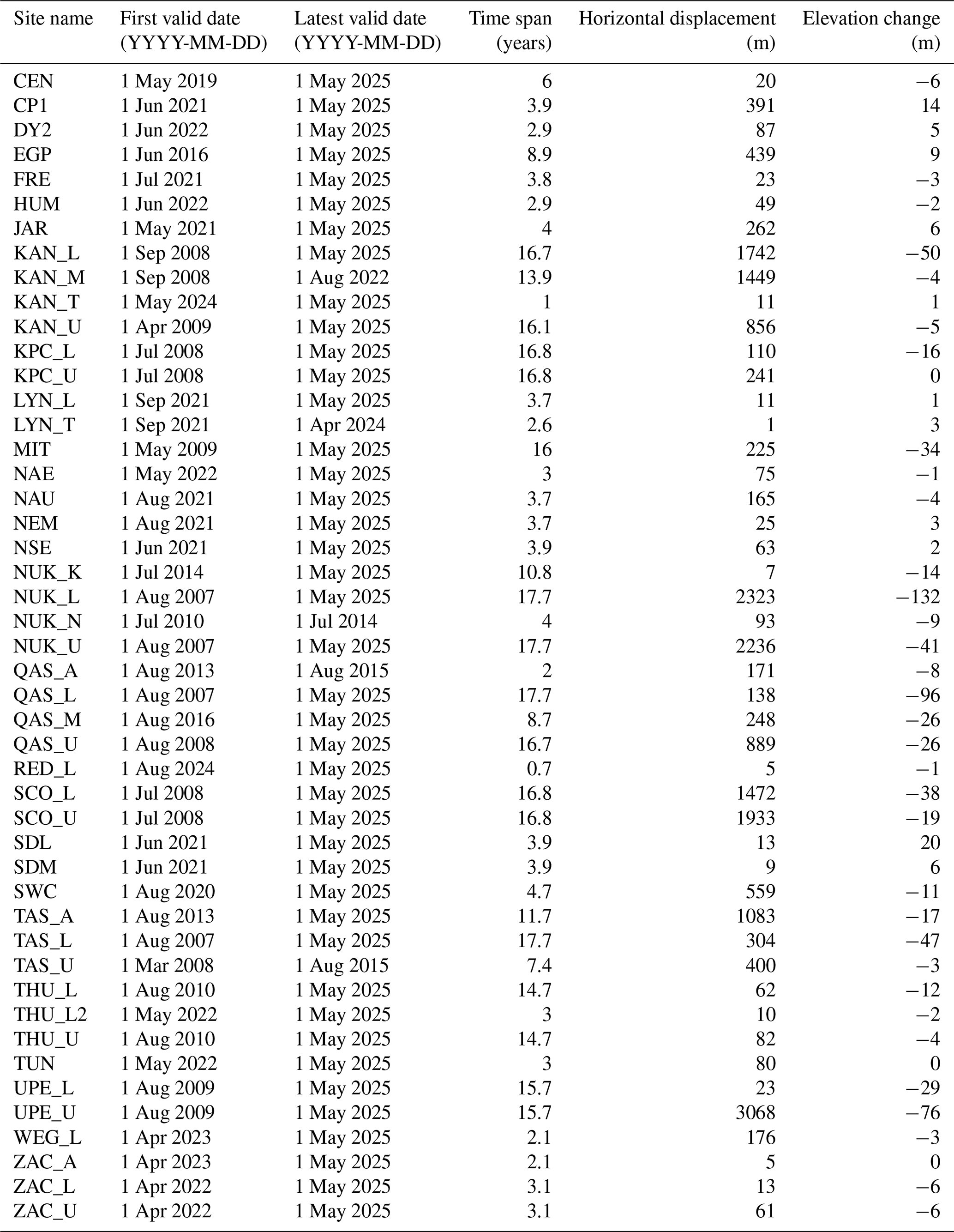
4.1 Time-dependent AWS position data

The AWS on ice are displaced over time by ice flow and surface ablation. The single-phase GPS available on all active stations provides relatively noisy data and occasionally has gaps. To provide continuous coordinates, we fit piecewise linear functions to the available GPS measurements and derive gap-free, smoothed positions for all timestamps. A discontinuity is introduced in these smoothed coordinates whenever the station is repositioned. An overview of the station displacements are provided in Table 7 and details on station repositioning during maintenance visit are provided in Sect. 4.2.

Historical GC-Net stations did not record continuous GPS positions. To address this, Vandecrux et al. (2023) compiled handheld GPS measurements and GNSS surveys collected during maintenance visits. For stations showing significant displacement and with sufficient point measurements, latitude and longitude were linearly interpolated. Sites with no position data (JAR2/JR2 and JR3), and sites with minimal vertical and horizontal displacement (less than approximately 10 m), such as Summit (SUM), SDL, SDM, NEM, and NGRIP (NGP), are represented by constant latitude, longitude, and elevation values.

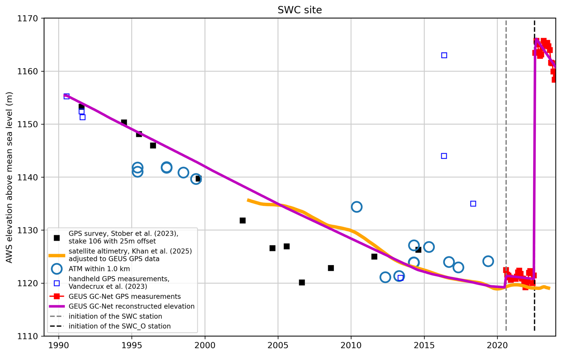
Figure 12 Example of reconstructed time-dependent site elevation at a historical GC-Net location, based on a linear fit to multiple elevation datasets including NASA ATM (from 1993), satellite altimetry (2003–2023), handheld GPS measurements, GC-Net onboard GPS data, and repeat geodetic surveys. The magenta line indicates the temporal interpolation used, with multiple interpolation points applied only at sites exhibiting multi-year variability such as Swiss Camp and JAR.

To represent elevation changes at historical GC-Net sites, which are important for applications such as barometric data assimilation in reanalysis, the time-dependent elevation of pre-GPS AWS data has been reconstructed using a combination of the following sources:

1. NASA Airborne Topographic Mapper (ATM) data beginning in 1993 (Thomas and Studinger, 2010; Studinger, 2014), within a 1 km horizontal search radius from daily horizontal position data (see Fig. 12),

2. Monthly satellite altimetry from 2003 to 2023 (Khan et al., 2025), for annually varying latitude and longitude,

3. A selection of handheld GPS measurements (see Table 7) (Vandecrux et al., 2023),

4. Monthly averaged GEUS carry-forward GC-Net onboard GPS data since 2020, in the case of Swiss Camp,

5. Repeat geodetic surveys from 1991 to 2022 for Swiss Camp and JAR (Stober et al., 2023).

Figure 12 illustrates the approach, where a linear function is fitted to the various elevation observations and interpolated temporally between points represented by magenta line. Only at Swiss Camp and JAR was it necessary to place multiple temporal interpolation points due to multi-year variability in site elevation caused by dynamic thickness changes. At other sites, a single linear temporal function was sufficient.

Table 8 AWS position changes for site relocations exceeding 90 m in horizontal distance. The table lists each affected site together with the month of the last data recorded before repositioning, the first full month after relocation, and the resulting horizontal displacement. Corresponding elevation changes are also provided to document vertical adjustments associated with each site move.

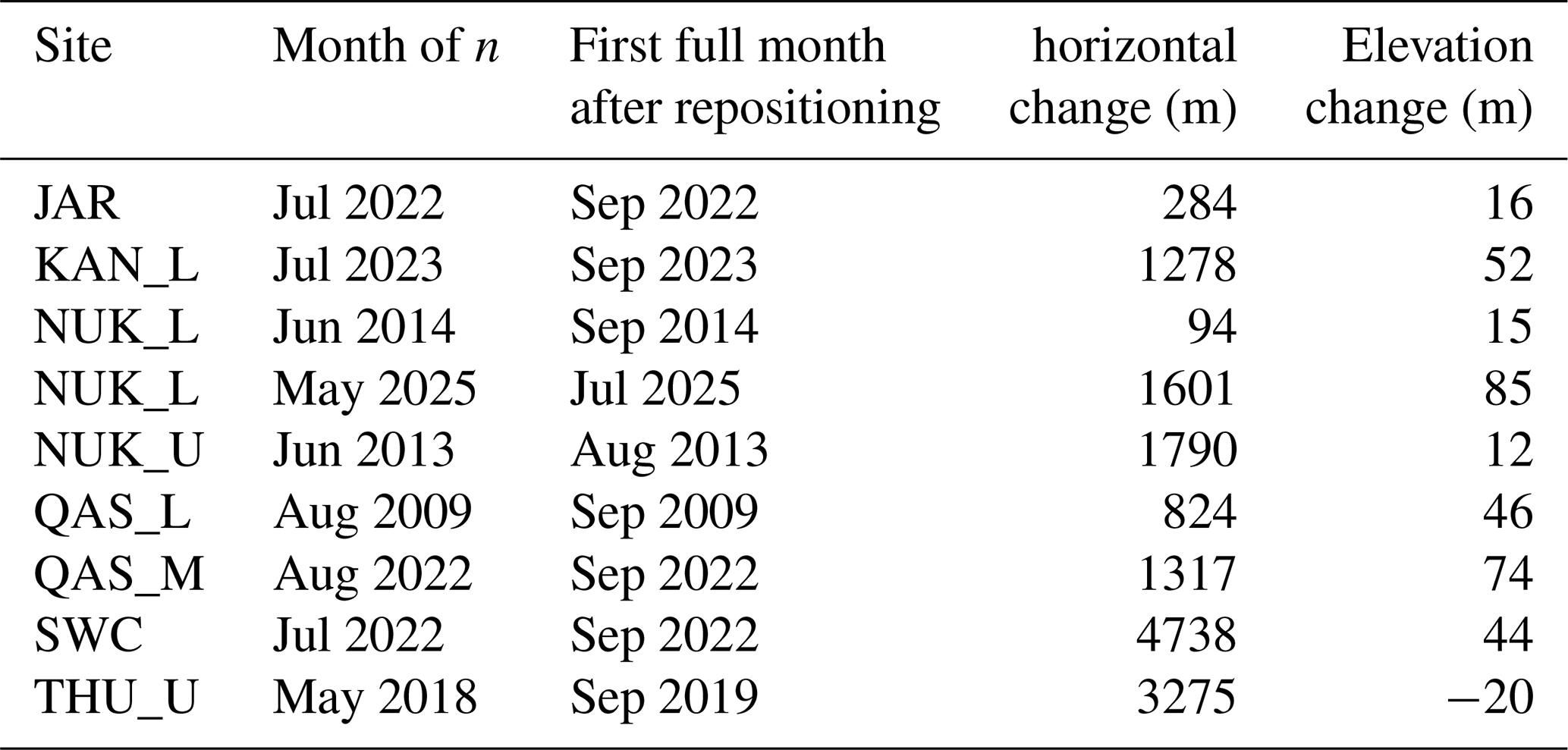
4.2 AWS reposition history

To date, stations JAR, KAN_L, NUK_L, NUK_U, QAS_L, QAS_M, SWC, and THU_U have been relocated during maintenance by distances exceeding 90 m horizontally (Table 8). Site repositioning has, for example, been carried out to avoid crevassed areas as in the case of the first year of QAS_L data or to mitigate recurrent station damage caused by excessive snowfall accumulation, as observed during the initial years at QAS_M. The Swiss Camp station, that had moved 4 km down glacier between 1990 and 2022, was replaced by the SWC_O station installed near (2.5 km north of) the 1990 position.

A total of 4961 h of concurrent data from the SWC and SWC_O stations, located 5.9 km apart, allowed for evaluating differences to test the assumption that the measurements represent a single site. Air temperature showed no significant difference, with a mean offset of 0.2 ± 0.6 °C. Surface air pressure differed by an insignificant 4.8 ± 4.8 hPa, and wind speed differed by 1.1 ± 1.6 m s⁻¹.

4.3 Surface Height Estimation from Multiple Sensors

Surface height is measured using multiple instruments. In this update, a new L3 variable, “z_surf_combined”, integrates data from several sensors to provide a continuous record of surface elevation, except during periods when all surface-ranging instruments fail. This variable also supports the estimation of time-varying thermistor depths used for subsurface temperature measurements (see Sect. 4.4). The method builds on approaches previously applied in scientific studies (Vandecrux et al., 2024).

At accumulation sites, surface height is derived from two sonic rangers mounted on the station booms. After correcting for height jumps caused by maintenance or mast adjustments, the two measurements are averaged to form z_surf_combined, reducing the influence of tilt, noise, and limited spatial coverage.

Tripod stations are equipped with three instruments:

• A sonic ranger mounted on the station,

• A sonic ranger mounted on a separate stake assembly,

• A pressure transducer installed in a borehole within an ablation hose (Fausto et al., 2012).

The station-mounted sonic ranger detects snow accumulation but cannot measure ice surface lowering during ablation, as the station descends with the ice. The stake-mounted ranger captures both snow accumulation and ice melt. Sonic ranger data are cleaned of errors, corrected for air temperature sensitivity where possible, converted to surface height, and adjusted to remove jumps from stake maintenance. The pressure transducer records only ice surface lowering and is unaffected by snow accumulation.

To construct z_surf_combined, the following procedure is applied:

• z_ice_surf is derived from z_pt_cor and manually adjusted after maintenance to ensure continuity.

• The ablation period is defined annually as the interval between the first and last weeks where z_ice_surf decreases. If unavailable, June–August is used.

• During ablation, z_surf_combined equals z_ice_surf, unless missing, in which case the stake-mounted ranger is used.

• At the end of ablation, sonic ranger readings are aligned with z_ice_surf, enabling snow accumulation tracking during winter.

• During the snow season, z_surf_combined is the average of the two sonic ranger measurements.

• In spring, as snow melts, surface height declines until it matches the ice surface height from the previous ablation season. From this point, the pressure transducer data are again used.

This procedure is adapted based on available data throughout the year. If all sensors fail during a period, surface height after the gap is manually set based on the trend observed in valid data. These interpolated values should not be considered direct observations, though the overall trend remains reliable. All surface heights are referenced to the initial station installation (i.e., zero height at installation).

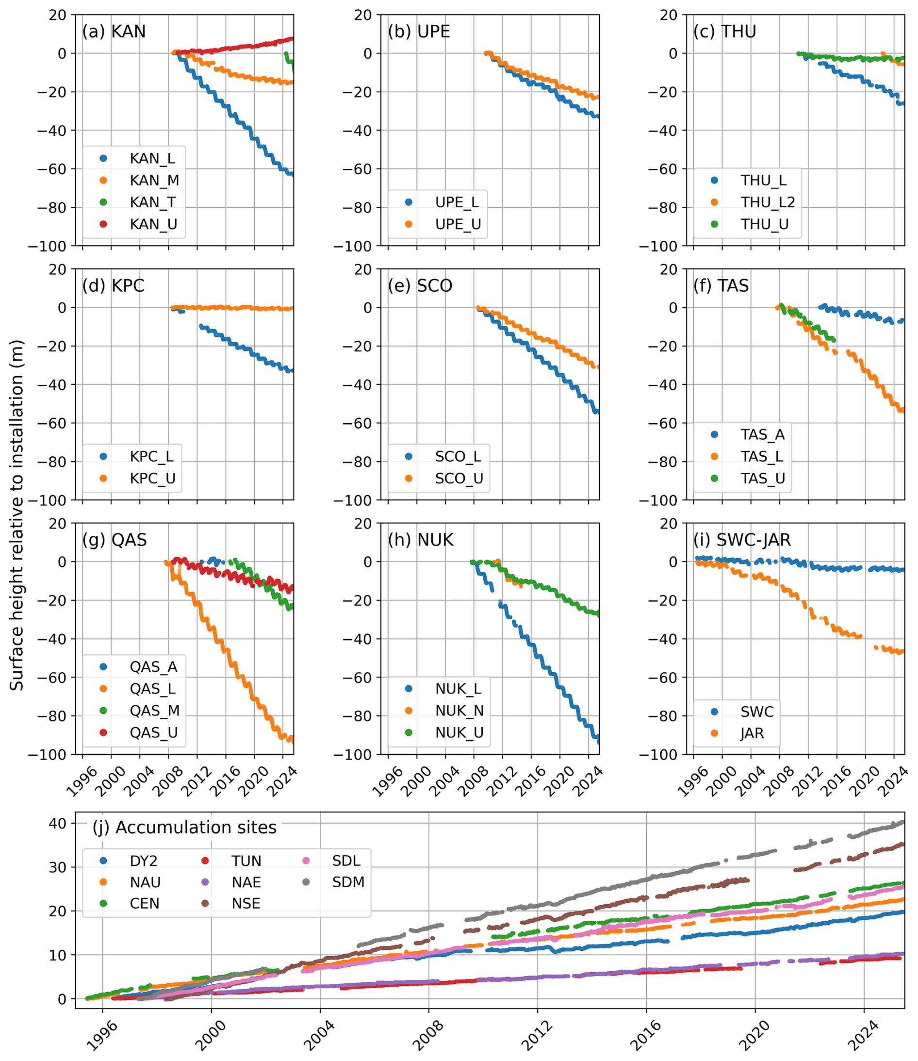
Figure 13 The integrated surface-height product (z_surf_combined) for all PROMICE and GC-NET sites. This variable merges observations from sonic rangers, pressure transducers, and stake-mounted sensors to produce a continuous elevation record that also supports estimates of time-varying thermistor depths.

From the resulting z_surf_combined (Fig. 13), z_ice_surf is recalculated as the 1 year lagging minimum of z_surf_combined. This ensures that z_ice_surf reflects ablation during summer and remains stable during winter. Finally, snow_height is computed as the difference between z_surf_combined and z_ice_surf, representing the snow depth above the ice surface. These two variables are provided only for ablation area sites.

4.4 Thermistor Depth Estimations and 10 m Ice/Firn Temperature Calculations

The thermistor strings measure temperature at depth at set intervals (e.g., every 1 m). At ablation sites the thermistor string slowly melts out and surfaces while at accumulation sites the thermistor string becomes buried. Thus, over time the initial depth at installation (noted in the raw data) is no longer the depth of measurement. This has been addressed in the following way: After we make our best estimation of the surface height, we can then specify the dates and depth of installation of thermistor strings to build a time-dependent depth variable for each thermistor. These depths are provided with the L3 data product and used to discard the recordings from surfaced thermistors which is common at the ablation stations. Once each temperature measurement has a depth tag, we can interpolate the firn/ice temperature at a standard 10 m depth. This standard depth has been used to be able to compare temporally and spatially various subsurface temperatures measurements (Vandecrux et al., 2024).

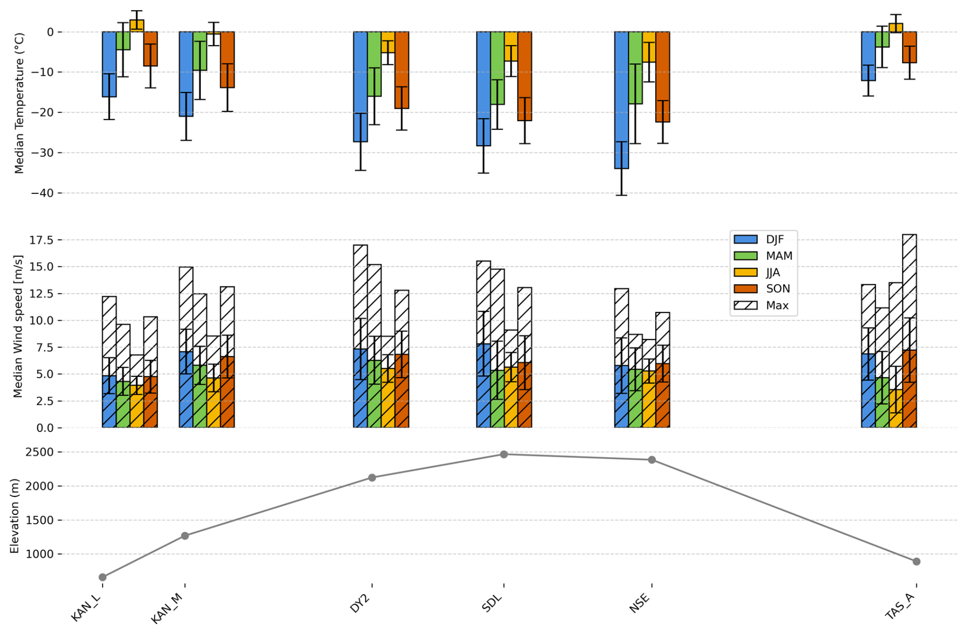
Figure 14 East–West transect from KAN_L to TAS_A showing seasonal meteorological conditions across ablation and accumulation areas. KAN_L, KAN_M, and TAS_A are located in the ablation area, while DY2, SDL, and NSE represent accumulation area stations. The upper panel shows median weekly air temperatures for each season, with black bars indicating the standard variability. The middle panel presents median weekly wind speeds, with hatched bars marking the maximum weekly wind speed for each season. The lower panel displays the elevation profile of the AWS transect.

4.5 Data Example

To provide some insight into the data product, we show examples of data from AWSs along two transects: one crossing the ice sheet East-West starting at the KAN_L station and ending at TAS_A (Fig. 14) and the other going South – North starting at the QAS_U station and ending at the KPC_U station. The transects include data from both types of weather stations. The East-West transect shows the seasonal medians and standard deviation of weekly means of temperature and wind speed observations (Fig. 14) across the ice sheet. Above freezing seasonal medians are observed at the lower stations during summer on both sides of the ice sheet, while the coldest temperatures are observed in the interior ice sheet. This is also where the highest median and maximum weekly wind speeds are observed. The exception to this is TAS_A on the East coast located in a region well-known for its piteraq storms (Van As et al., 2014b). This is reflected in the high maximum windspeeds found in summer and fall as well as high variability.

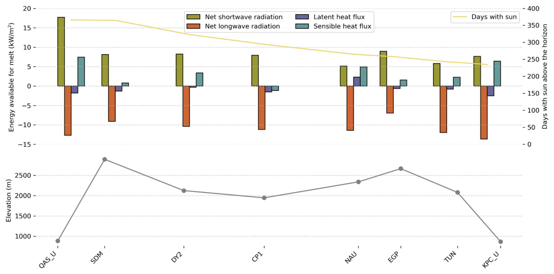
Figure 15 Annual mean surface mass balance components for a South–North transect using all available data. Stacked bars show net shortwave and longwave radiation, latent and sensible heat fluxes, and the resulting energy available for melt at each station. The yellow line indicates the annual number of days with the Sun above the horizon. The lower panel displays station elevations along the transect.

The South–North transect displays the major components of the surface energy balance (Fig. 15). Net shortwave radiation is the downward minus upward irradiance, which in principle, is always positive and highly dependent on the surface type. The sites in the ablation area will be on a bare ice surface with a much lower albedo than the sites in the accumulation area where the surface is snow covered. The net shortwave irradiance is furthermore affected by the total number of days where the sun is above the horizon, visualized by counting all the days with downward shortwave radiation higher than 1 W m⁻² (Fig. 15). The net longwave irradiance is on average negative, which means that the ice sheet is emitting more longwave radiation than it receives from the atmosphere and this means a cooling of the snow/ice. The latent turbulent heat flux is an energy exchange due to the phase changes of water at the ice sheet surface. The mean value is negative at most sites, meaning that evaporation or sublimation is removing energy from the surface. At NAU latent turbulent heat is however positive which means that the moisture in the air is condensing on the ice sheet and thereby imparting heat to the surface. Finally, the total energy from sensible turbulent heat flux is positive at all sites except for CP1. The sensible turbulent heat flux is the transfer of heat between the air and the ice sheet surface due to the temperature difference carried by moving air. When sensible heat flux is positive the air is warmer than the surface and the surface is being heated by turbulent transfer. When sensible heat flux is negative the ice sheet releases heat to the air.

5 Living Data and Continuous Improvements

The PROMICE | GC-NET programmes will continue to update and distribute data products as AWS data becomes available. There may be undiscovered issues in the current dataset, and new challenges could emerge in future data collections.

Living data and FAIR principles

The PROMICE | GC-NET AWS data are managed in accordance with the FAIR principles (Wilkinson et al., 2016). All datasets are permanently archived in recognized open repositories and assigned persistent identifiers (DOIs). Each dataset is accompanied by rich, machine-readable metadata conforming to CF conventions where applicable (Eaton et al., 2024), including station identifiers, geographic coordinates, instrumentation details, sampling intervals, measurement units, and version history. Data are distributed in community-standard formats such as NetCDF (Rew and Davis, 1990; Unidata, 2023) with CF metadata and CSV with machine-readable headers, and they use controlled vocabularies and standardized units such as CF standard names to ensure interoperability. Access is open under the CC-BY 4.0 license. Provenance and processing history, including quality-control flags and software version information, are fully documented. Users are requested to cite the dataset using the assigned DOI and recommended citation format. When updates occur, dataset versions are tracked, and previous versions remain publicly accessible and discoverable at https://doi.org/10.22008/FK2/IW73UU (How et al., 2022a).

Table 9 Overview of known AWS data issues grouped by category. Frequency refers to how commonly the issue has been observed across PROMICE and GC–NET stations, and typical consequences describe impacts on the resulting dataset.

6 Operational Challenges and Key Lessons Learned

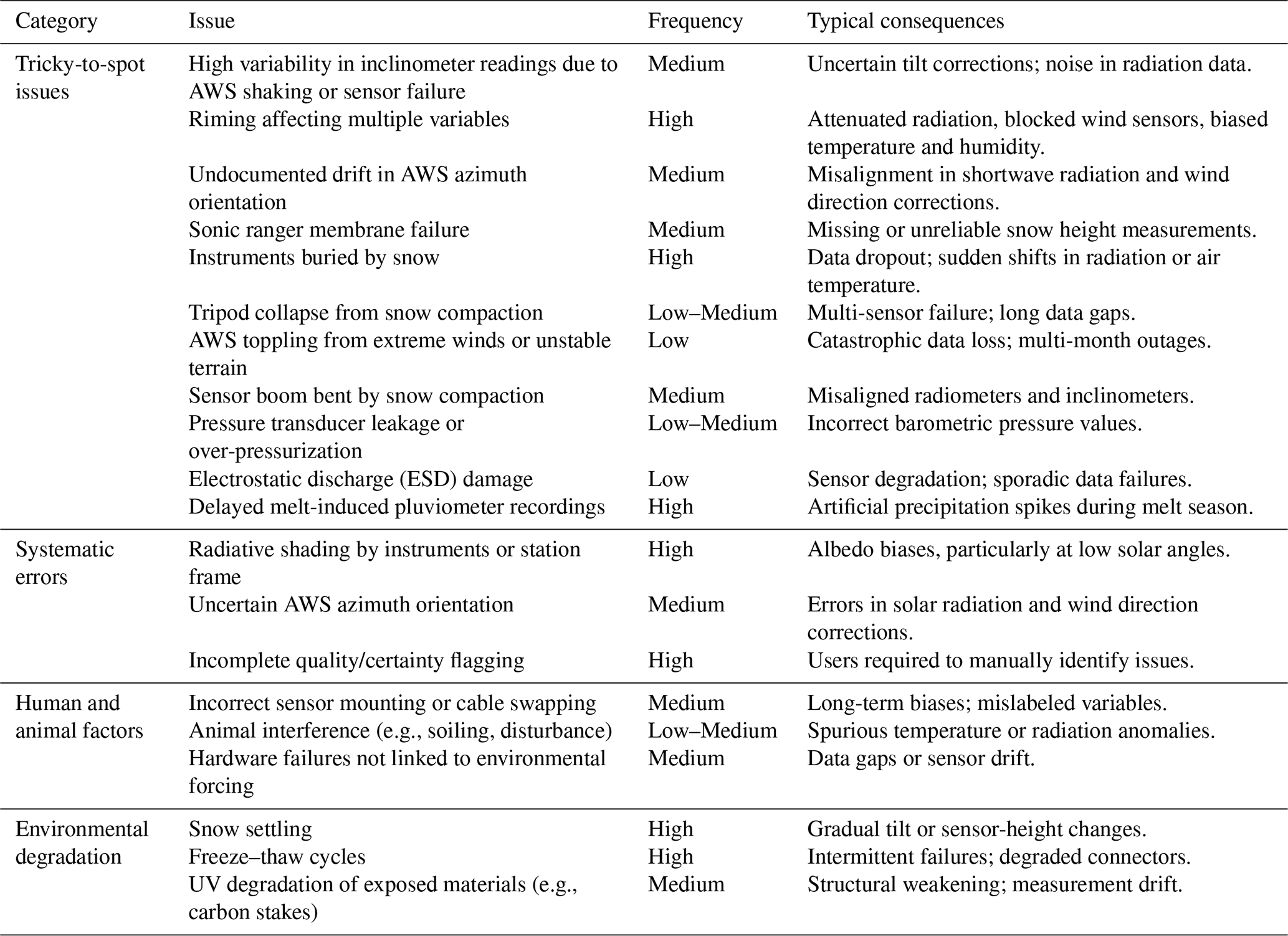
Long-term operation of the PROMICE | GC–NET automatic weather stations (AWSs) has revealed a wide spectrum of data-quality issues arising from environmental conditions, instrument limitations, installation geometry, and human or animal interaction. Numerous individual issues have been catalogued across the network. Table 9 summarizes these issues by type, while this section provides a concise synthesis of the most frequent challenges and the practical experience gained from addressing them in both fieldwork and post-processing.

6.1 Tricky-to-detect issues

Several issues develop gradually and therefore require multi-variable inspection or contextual knowledge to diagnose. Riming is among the most common wintertime phenomena, periodically affecting temperature, humidity, wind speed, and radiation measurements. It often manifests as suppressed shortwave irradiance peaks, artificially smooth wind records, or persistent sensor icing that masks natural variability.

Instrument burial is also frequent at sites with substantial winter accumulation. Radiometers and sonic rangers may become partially or fully submerged, causing abrupt changes in measured radiation or snow height. Slow variations in station azimuth or tilt, caused by storms, snow compaction, or deformation of supporting structures, occur less often but can introduce systematic errors into shortwave radiation corrections and wind-direction measurements. At one site, an apparent inclinometer drift over several months, initially interpreted as sensor noise, was later confirmed through field photographs to reflect actual bending of the sensor boom by compacting snow.

6.2 Systematic errors

Certain issues recur with sufficient regularity to be considered systematic across the PROMICE | GC–NET stations. Radiative shading from the station frame is a consistent source of bias, especially during periods of low solar elevation. The severity of shading varies with station geometry and seasonal surface height and can lead to systematic underestimation of reflected shortwave radiation and albedo.

AWS azimuth orientation is another persistent challenge. While azimuth is documented at installation and during maintenance visits, storm-induced rotation, tilt changes, or creeping motion may occur between site visits. Uncertainties in azimuth propagate directly into shortwave radiation corrections and wind-direction analyses. Earlier versions of the dataset lacked comprehensive metadata and standardized quality flags; these are being expanded to improve traceability and facilitate user-side assessment of data reliability.

6.3 Human, animal, and environmental influences

Human and animal interactions, though less common than environmental drivers, contribute to several documented issues. Occasional sensor misalignment, incorrect mounting height, and rare cable swapping during rapid maintenance can produce detectable biases or abrupt transitions in the data. Such cases are typically identified through cross-variable consistency checks.

Animal interference is sporadic but observed at several stations, mainly due to Arctic fox activity. This includes soiling of radiometers, disturbance of pressure inlets, or minor displacement of sensors.

Environmental degradation processes are pervasive across the network. Snow settling alters sensor heights and station tilt; freeze–thaw cycles degrade electrical connectors and enclosures; and long-term ultraviolet exposure weakens materials such as carbon stakes and sensor mounts. Several stations have experienced small but measurable orientation shifts after repeated melt seasons due to material fatigue.

6.4 Illustrative examples

Three representative cases highlight the range of issues encountered:

1. Progressive inclinometer drift during a winter season was later shown, via field photography, to reflect actual deformation of the sensor boom caused by snow compaction.

2. Delayed rainfall events at the onset of multiple melt seasons were produced by melt-out of snow accumulated inside the pluviometer rather than by new rain.

3. A storm-affected maintenance visit resulted in inadvertent swapping of temperature and wind-speed sensor cables, later identified in post-processing through anomalously similar diurnal cycles.

These examples underscore the importance of cross-variable inspection, robust metadata, redundant observations where possible, and consistent photographic documentation during field visits.

To support transparency and collaboration, we maintain a user-contributable web-based database of known data quality issues at: https://github.com/GEUS-Glaciology-and-Climate/PROMICE-AWS-data-issues (last accessed: 7 April 2025). This system uses GitHub “issues” to log problems and challenges, with each entry tagged by relevant station, sensor, and year. Users are encouraged to check the database for known issues related to their specific use of the dataset. If a new issue is identified, users can report it directly in the database. A PROMICE | GC-NET team member will review and verify the issue, mark it as confirmed, and suggest a correction if appropriate. Verified issues will be addressed in future data releases. All issues remain accessible, even after they are closed.

7 Data availability

The PROMICE | GC-NET AWS dataset is primarily available through the GEUS Dataverse (https://doi.org/10.22008/FK2/IW73UU), which is updated monthly (How et al., 2022a). This version of the dataset has undergone both automatic and manual quality control protocols.

Near-real-time PROMICE | GC-NET AWS data can be accessed from the GEUS Thredds server (https://thredds.geus.dk, last access: 12 November 2025), which serves as an OPeNDAP access point for our operational datasets. The PROMICE | GC-NET AWS dataset is updated hourly with the latest transmission measurements from the station network. These measurements are collected, processed, and delivered to the GEUS Thredds server with a latency of approximately 10–15 min.

8 Summary

The updated PROMICE | GC-NET automatic weather station (AWS) data product provides a comprehensive overview of the AWS network that monitors the Greenland Ice Sheet. This release focuses on key advancements in station design, instrumentation, and the data processing workflow that together improve the quality, reliability, and scientific value of the observations.

Two primary AWS station designs are used across the network: the accumulation area mast stations and the ablation area tripod stations. Accumulation area stations are constructed with a two-boom mast drilled into the firn and are optimized for long-term stability in high-accumulation regions. These stations measure atmospheric parameters at two vertical levels, which is essential for calculating turbulent fluxes. The ablation area stations, on the other hand, are designed around a one-boom free-standing tripod system that is lightweight and ideal for deployment in the low-elevation ablation zones where surface melting dominates. The tripod system rests on the ice surface and includes features like a suspended battery box to improve stability.

Substantial updates have been made to the instrumentation of both station types. Air temperature and humidity measurements now rely on high-precision sensors such as the Vaisala HMP155E and OTT Lufft WS401, which are housed in fan-aspirated radiation shields to reduce solar heating errors. Radiative fluxes are measured using Kipp & Zonen CNR4 radiometers, replacing older models and enabling higher accuracy through better thermal stability and integrated tilt correction. Measurements of snow accumulation and ice ablation are made using paired sonic rangers and pressure transducer assemblies. These are further enhanced by structural changes to reduce issues like melt-out of stakes. Subsurface temperature profiles are obtained using analog and digital thermistor strings, with depths extending to 10 m. AWSs are powered by a combination of solar panels and battery systems (both lead-acid and NiMH), and data transmission is handled via the Iridium Short Burst Data system to ensure global coverage even in remote polar regions. Data loggers have been upgraded to the CR1000X model, offering improved speed, memory, and analog accuracy over the CR1000 logger.

Central to this release is the adoption of a robust, open-source data processing framework called pypromice. This Python-based workflow processes raw and transmitted data through several levels. Level 0 consists of raw measurements retrieved directly from the data loggers or received via satellite transmission. Level 1 converts these readings into physical units using calibration coefficients. Level 2 applies automated and manual filtering routines to remove outliers, correct persistent values, and flag suspect data based on known maintenance activities. Level 3 provides the final, user-ready dataset with both measured and derived variables, including specific humidity, surface temperature, turbulent energy fluxes, cloud cover, and albedo.

The workflow accommodates both station formats and merges records from station upgrades or replacements to form long-term continuous datasets at each geographic site. This ensures data continuity and supports analyses over decadal timescales. Following the FAIR principles, the data products are available in both CSV and CF-compliant NetCDF formats, catering to a wide range of users. Public participation in data quality assurance is encouraged through an open GitHub repository, allowing researchers to flag issues or suggest corrections, which are reviewed and incorporated by the PROMICE | GC-NET data team.

In summary, the PROMICE | GC-NET AWS data product update represents a significant advancement in Arctic climate monitoring. Through enhanced station designs, state-of-the-art instrumentation, and a transparent, automated data processing workflow, the dataset offers an essential resource for studying the Greenland Ice Sheet and its periphery, validating climate models, and supporting global assessments of cryospheric change.

Appendix A: Instrument specifications

This appendix provides an extended overview of the weather-station instruments referenced in the dataset description. It compiles manufacturer-specific documentation for each sensor and logger, including model names, hardware revisions, measurement principles, operational ranges, and accuracy specifications. Additional tables summarize environmental tolerances, power requirements, maintenance considerations, and known performance limitations. Together, these details support transparent interpretation of the meteorological observations, enable reproducibility, and facilitate comparison across different instrument types or deployment sites. The appendix is intended as a technical reference for researchers, data users, and system operators who require a deeper understanding of the equipment underlying the dataset.

Thermometers (aspirated)

The Rotronic RS12T contains a Pt100 temperature probe and separate hygroclip, which also incorporates a temperature probe (see Table A6). The probes are housed within an RS12T aspirated weather and radiation shield. The white shield minimises the influence of thermal radiation on temperature (and humidity) measurements, and additionally provides protection against horizontally driven rain and snow. Older generations of the tripod system as described in Fausto et al. (2021) use the Rotronic (Table A3), while the newer generations use the OTT Lufft WS401. In contrast, older generations of the mast sysem use OTT Lufft WS401, while newer generations use Vaisala HMP155E with a Rika aspirated fan.

Table A1 Manufacturer-specific documentation for Campbell Scientific CS100 (also known as Setra 278), which is used for newer generations of the mast system and older generations of tripod system (Table A1).

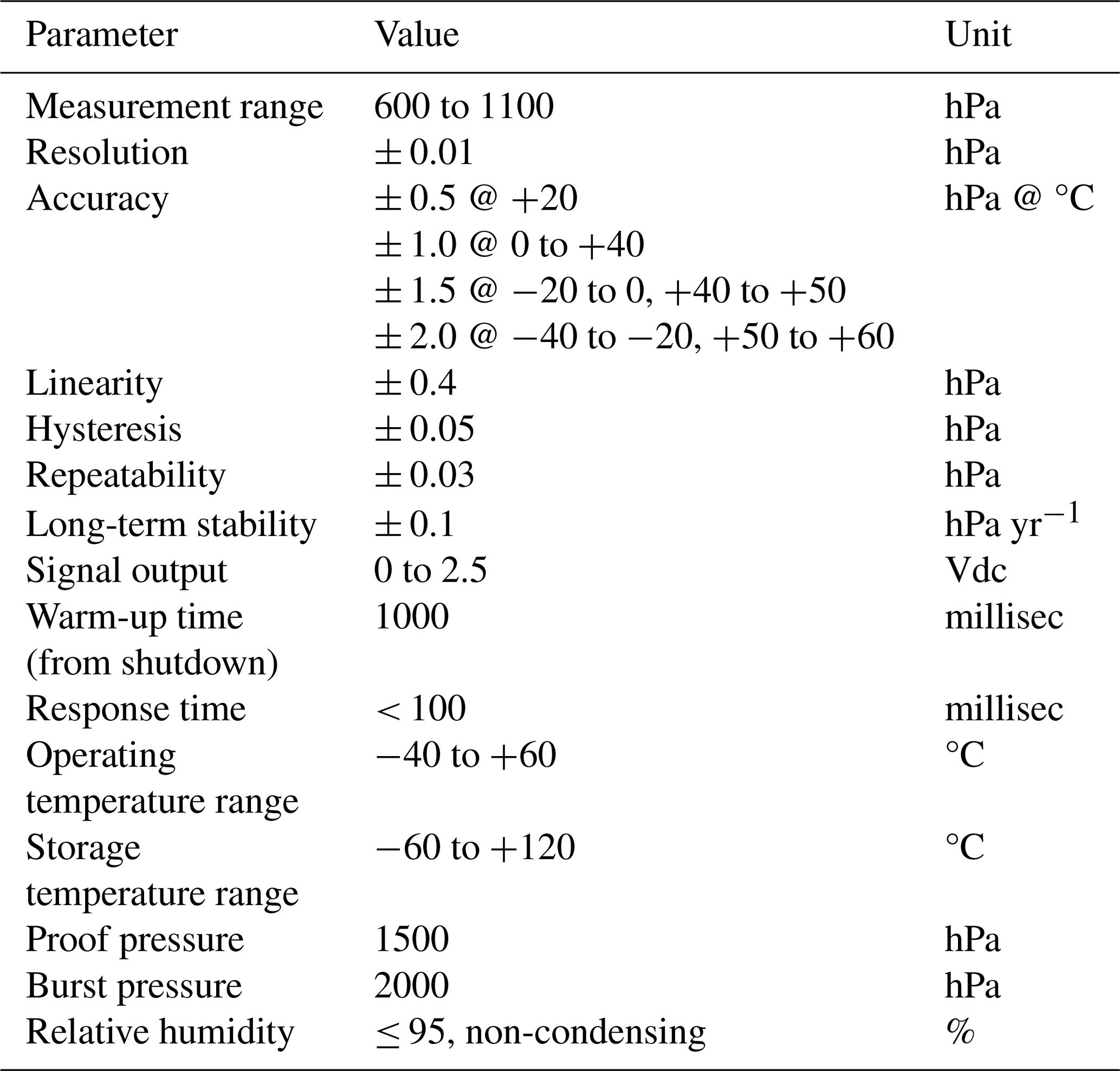
Table A2 Manufacturer-specific documentation for OTT Lufft WS401, which is used for newer generations of the tripod system and older generations of mast system (Table A2).

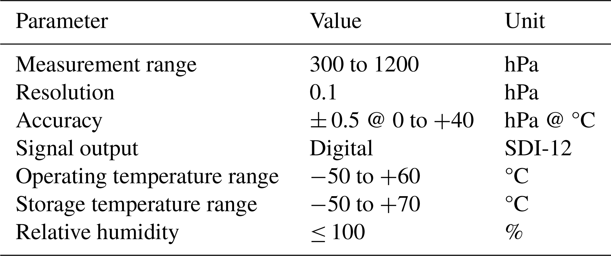
Table A3 Manufacturer-specific documentation for Rotronic Hygroclip HC2/HC2 and S3 Pt100.

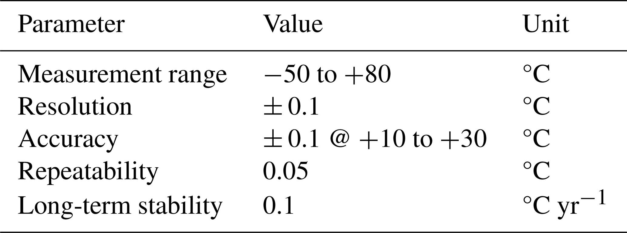
Table A4 Manufacturer-specific documentation for OTT Lufft WS401 (thermometer parameters).

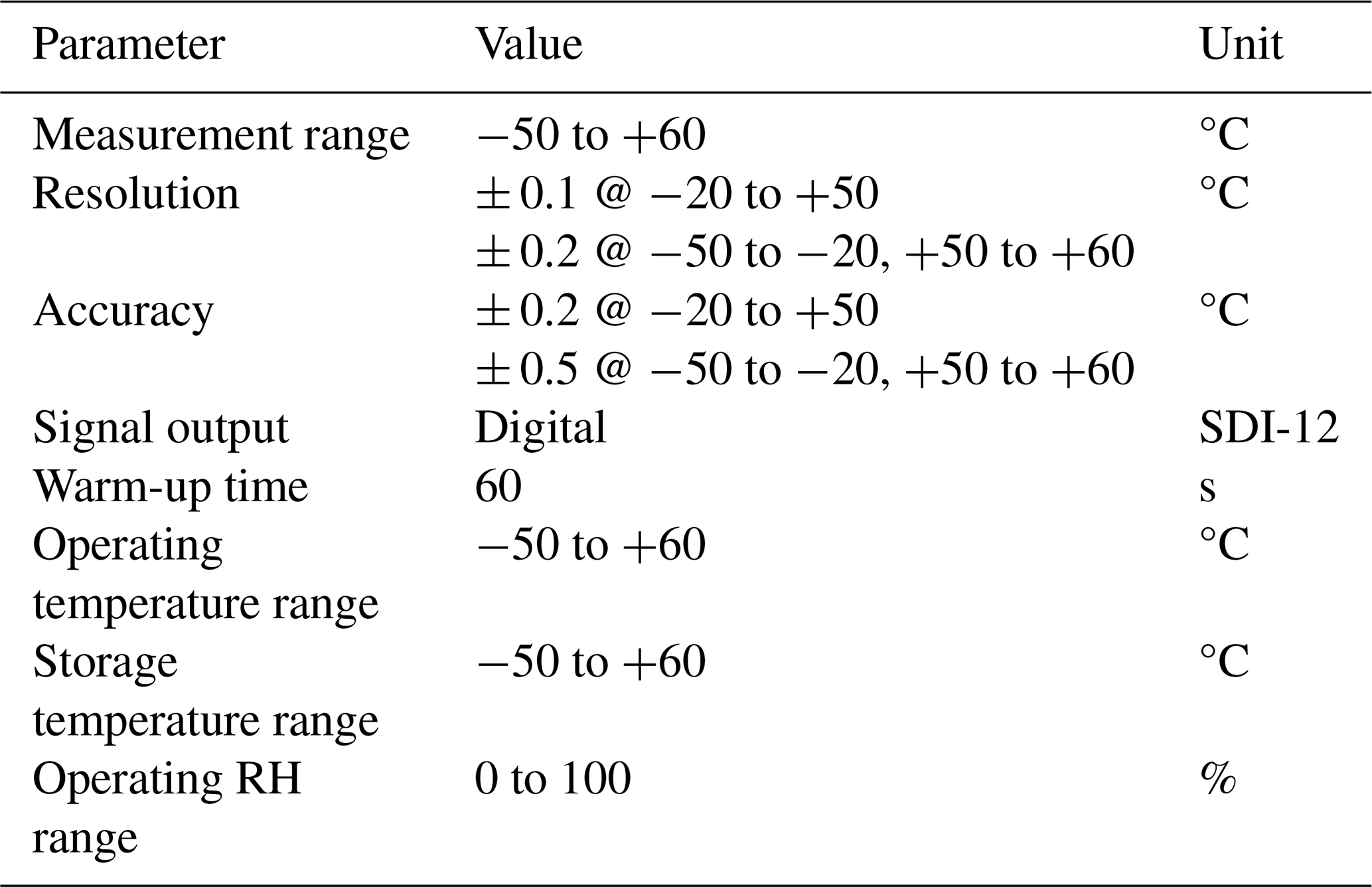
Table A5 Manufacturer-specific documentation for Vaisala HMP155E (thermometer parameters). Uses a Rika aspirated fan.

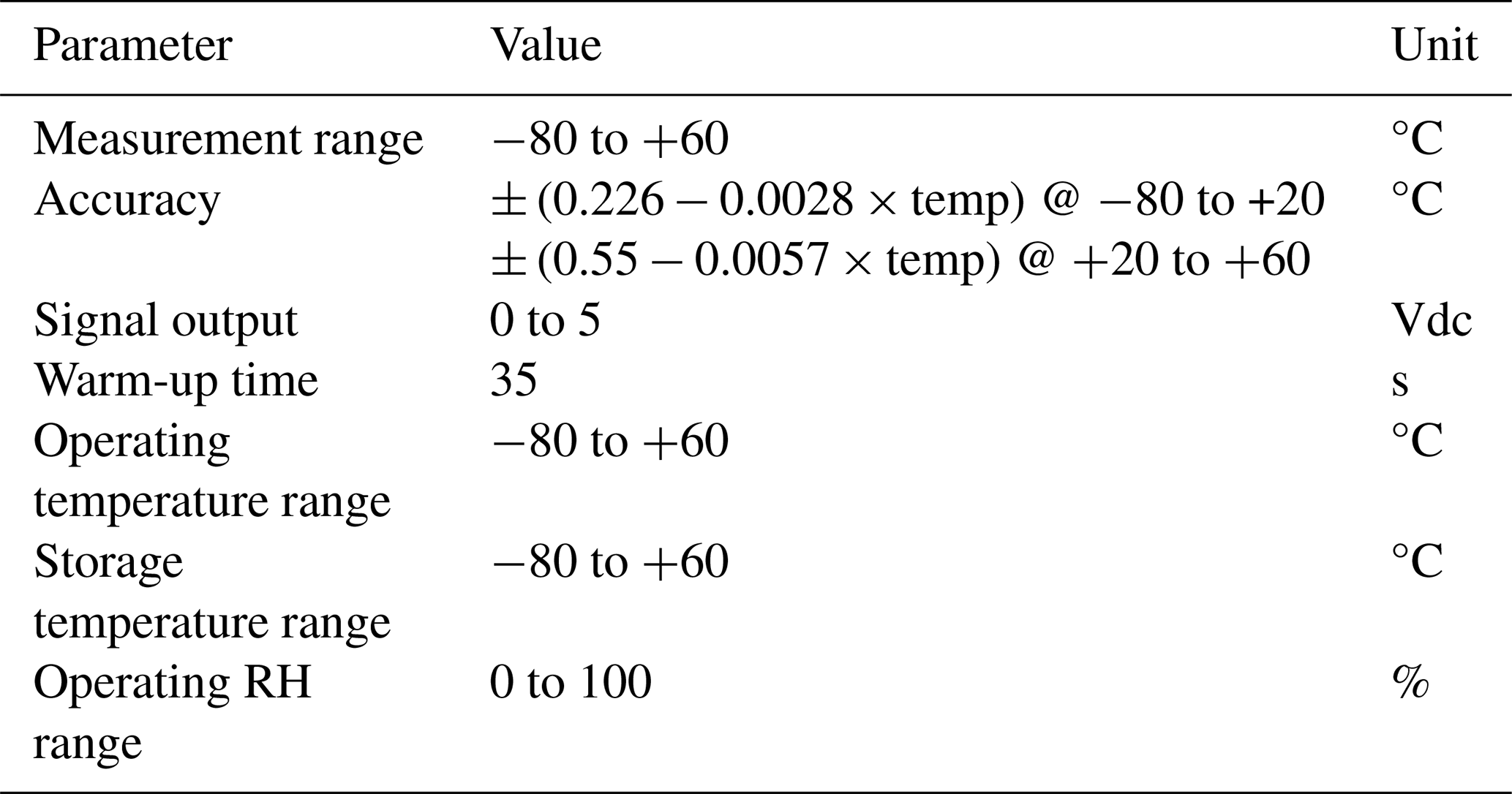
Hygrometers (aspirated)

Table A6 Manufacturer-specific documentation for Rotronic Hygroclip HC2/HC2-S3.

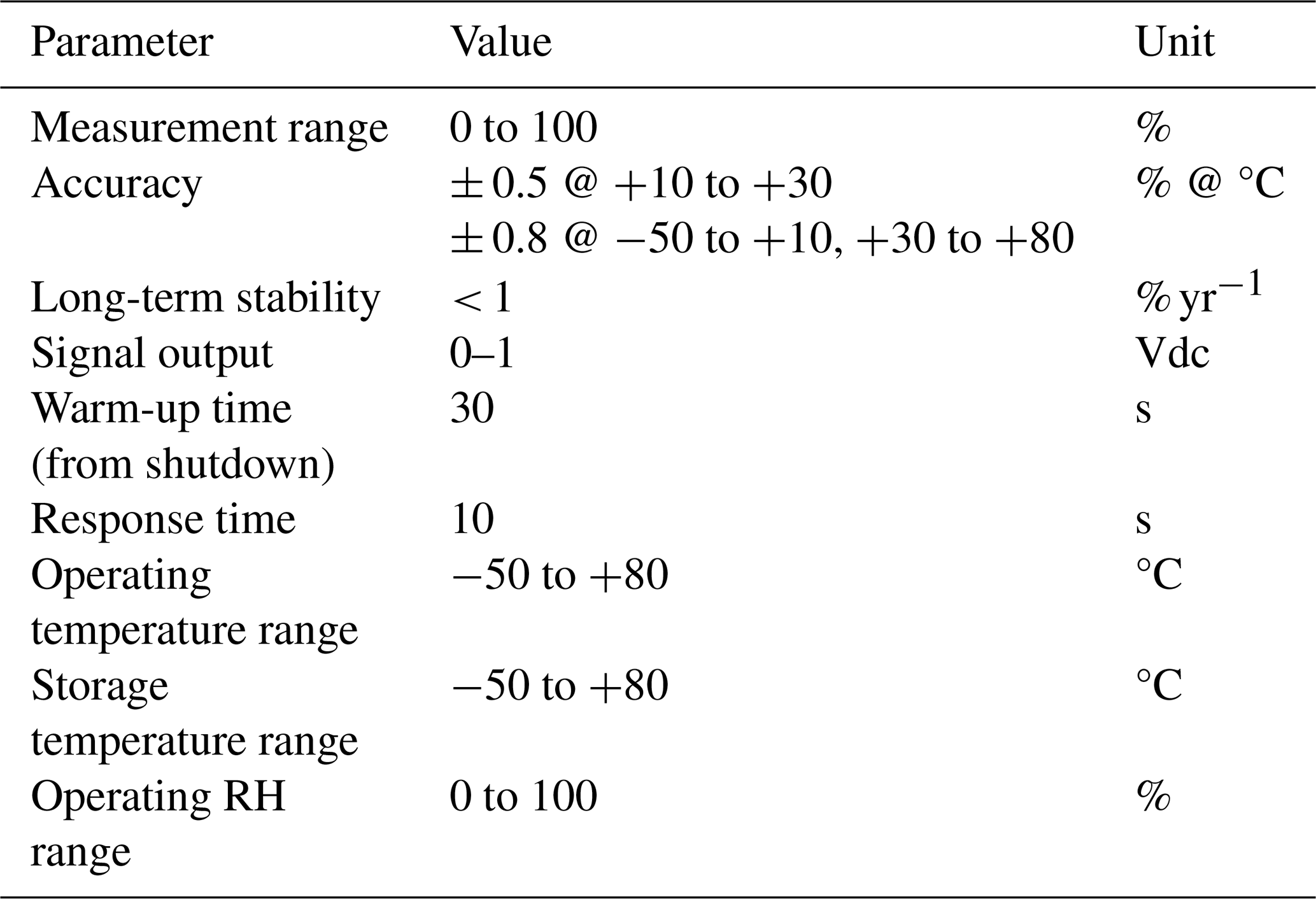
Table A7 Manufacturer-specific documentation for OTT Lufft WS401.

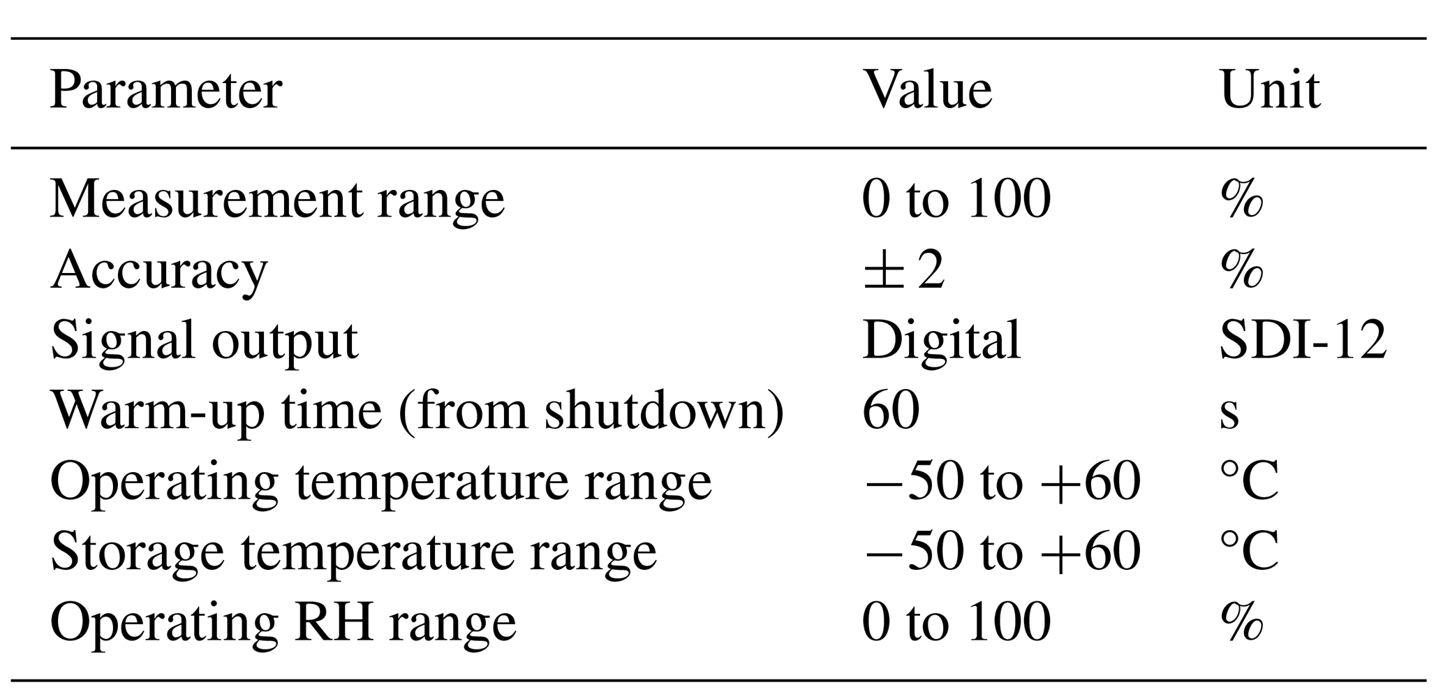
Pluviometer

Table A8 Manufacturer-specific documentation for OTT Lufft WS401 (pluviometer parameters).

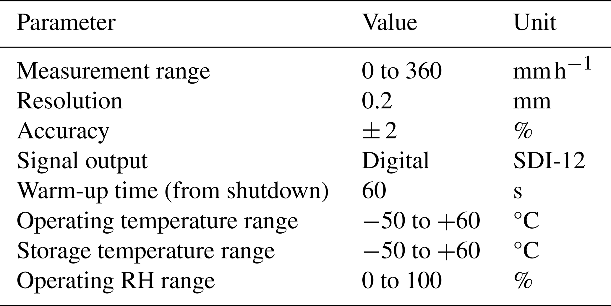
Anemometers

Technical specifications for the R.M. Young 05103 and 05108 HD-Alpine propeller–vane anemometers used in this study. Both instruments provide co-located wind speed and wind direction measurements based on a mechanical propeller and tail vane system. The HD-Alpine model includes reinforced components and an extended temperature range for operation in harsh, icing-prone environments. Parameter definitions and units follow the manufacturer's documentation in Tables A9 and A10.

Table A9 Manufacturer-specific documentation for Young 05103.

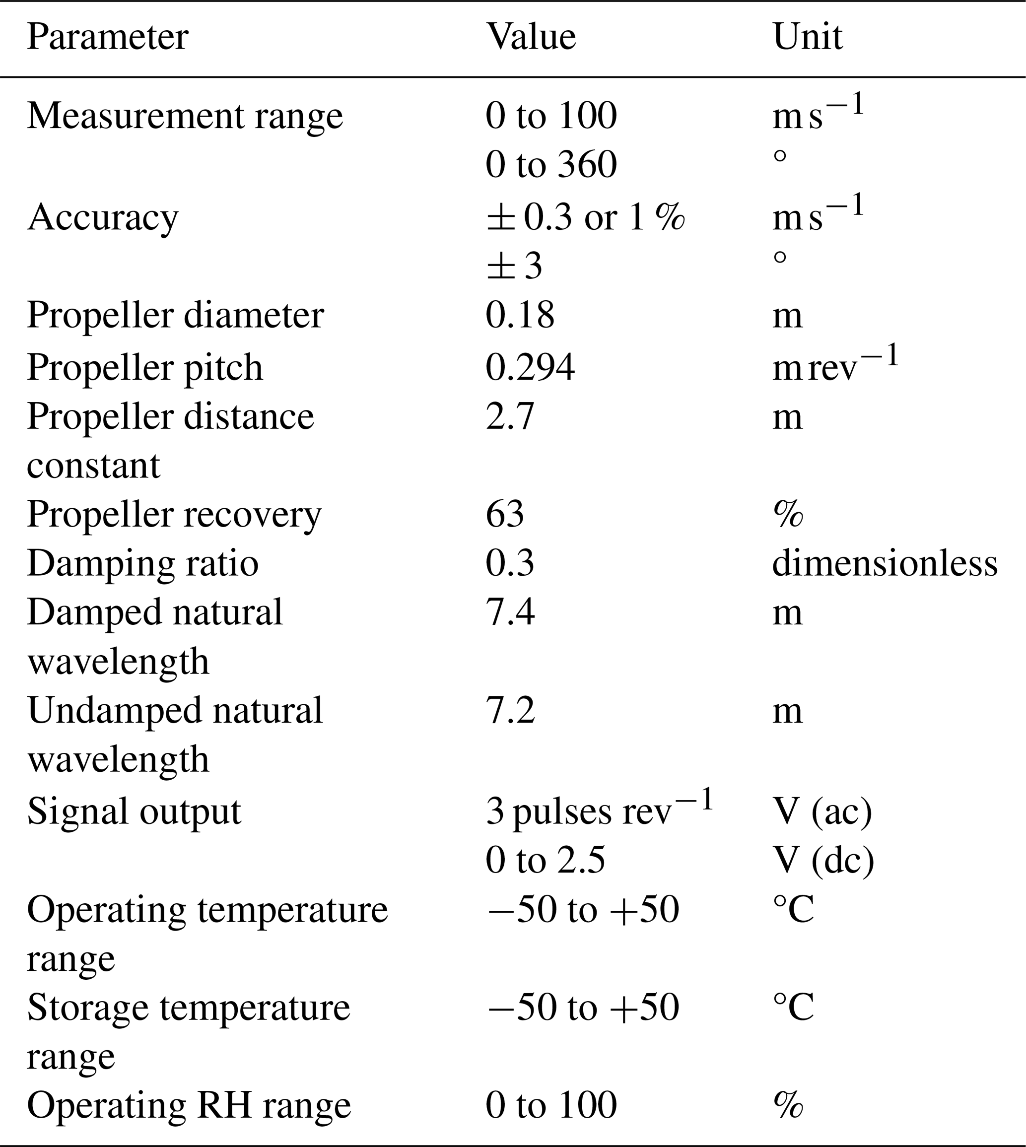
Table A10 Manufacturer-specific documentation for Young 05108 HD-Alpine.

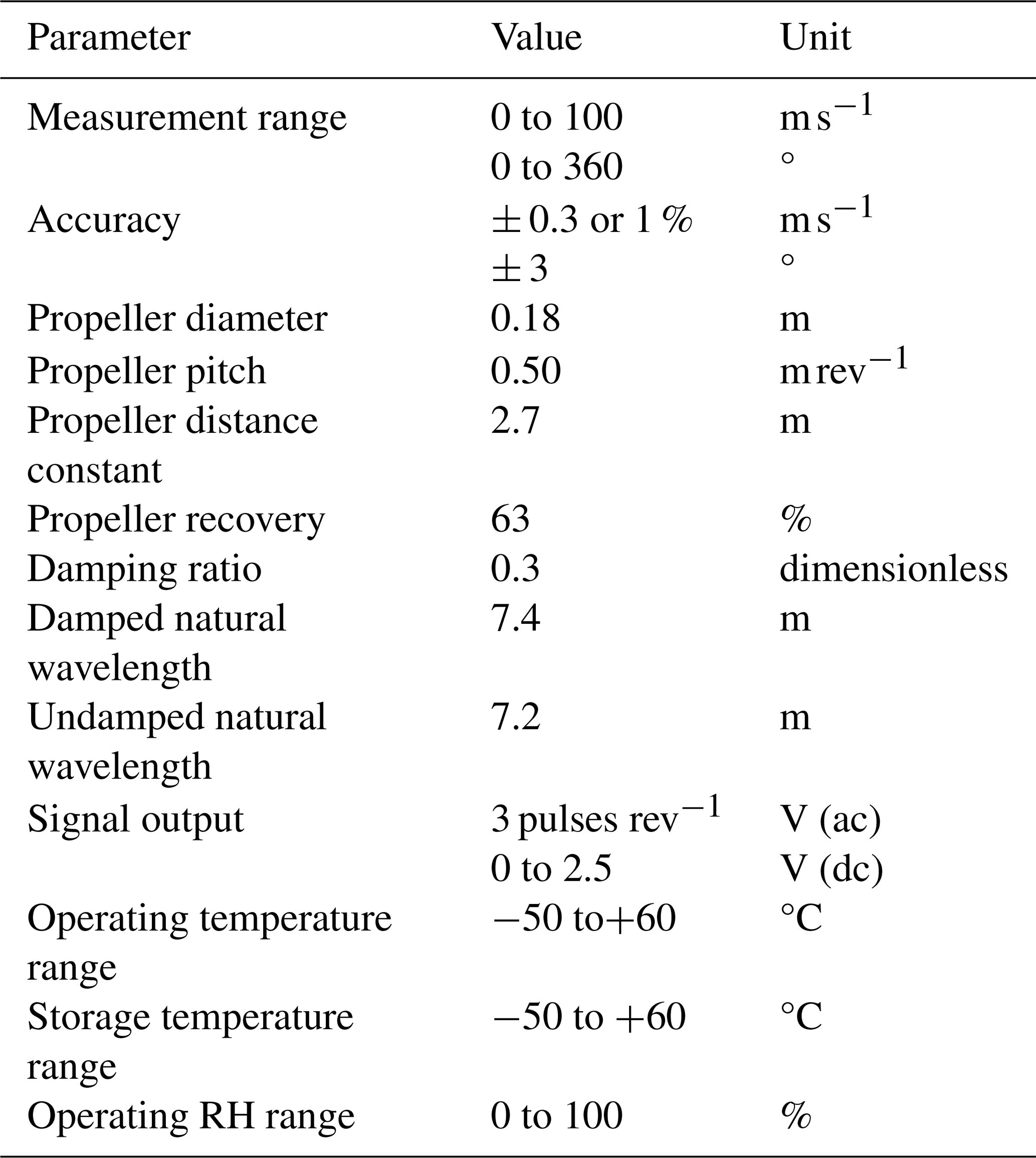
Net Radiometers

Each net radiometer is comprised of up- and down-facing pyranometers and pyrgeometers (i.e., 4 individual sensors). If the sensor type is not specified in the tables below, the value applies to all sensors.

Table A11 Manufacturer-specific documentation for Kipp and Zonen CNR 4.

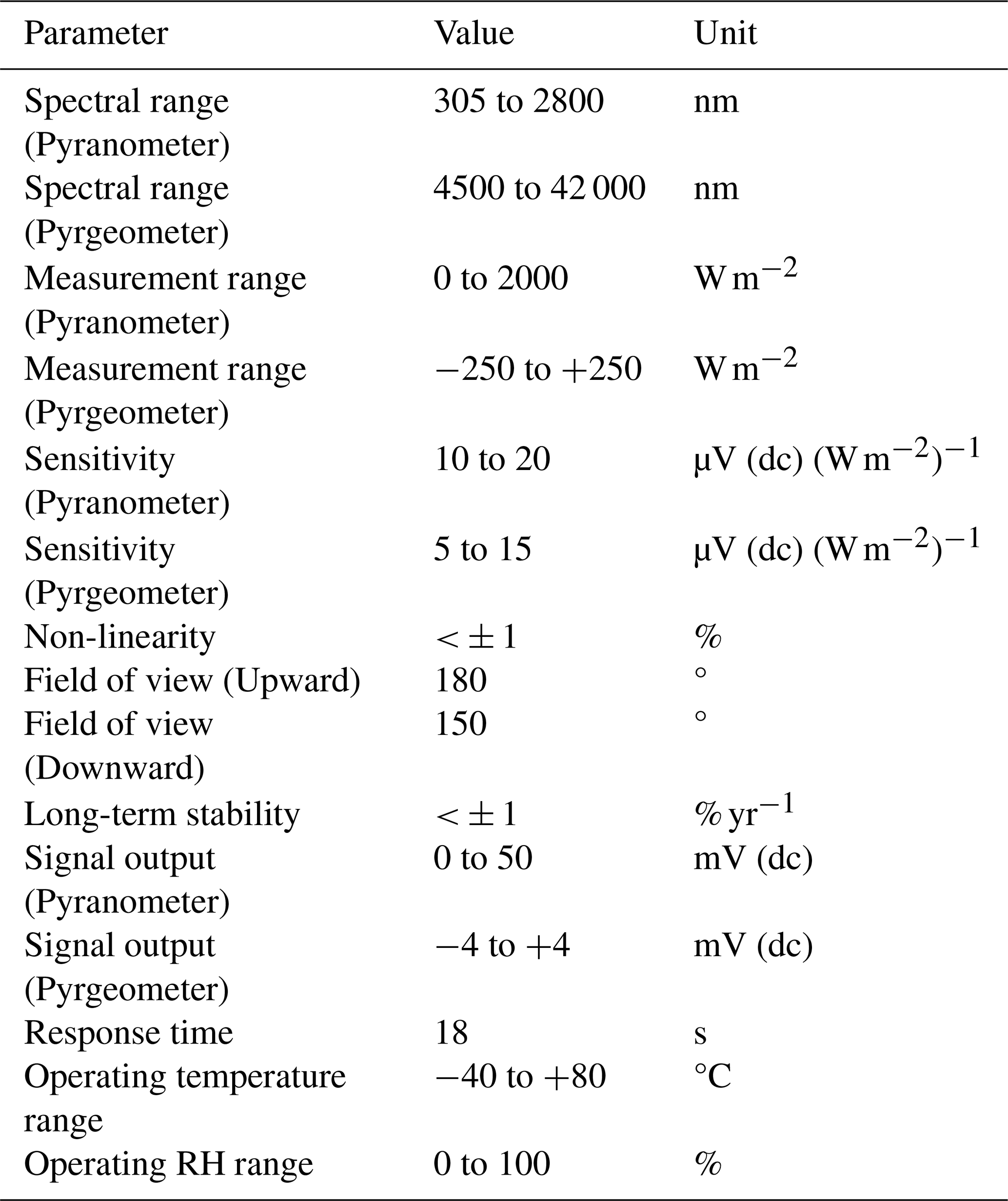
Table A12 Manufacturer-specific documentation for Kipp and Zonen CNR 1.

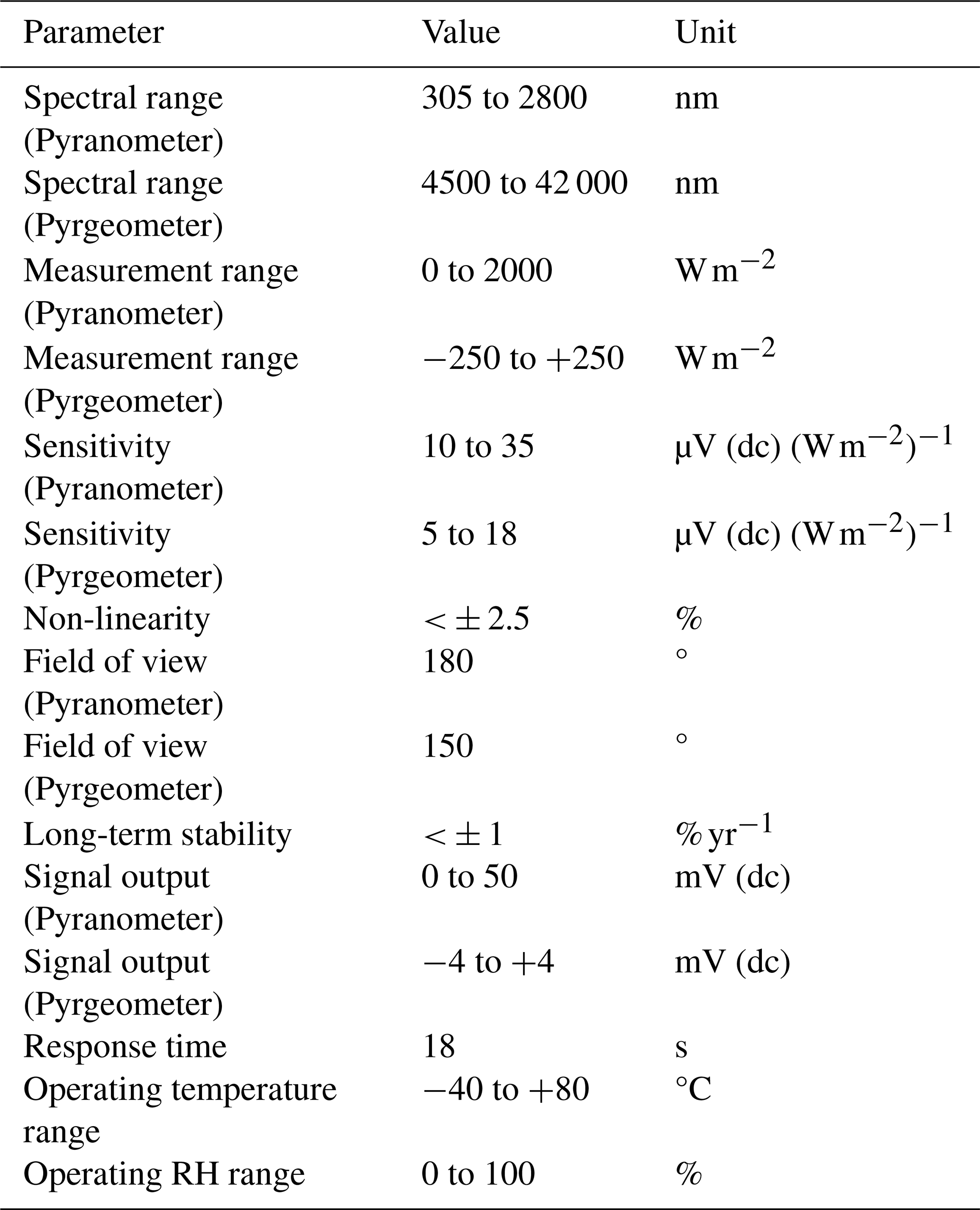
Sonic Ranger

Table A13 Manufacturer-specific documentation for Campbell Scientific SR50 ultrasonic distance sensor used for measuring snow depth. The SR50 determines the distance to the surface by emitting a 50 kHz ultrasonic pulse and measuring the elapsed time to the returned echo. Because the speed of sound varies with air temperature, the sensor requires an external temperature measurement for compensation. The SR50 is capable of detecting small or acoustically absorptive targets such as low-density snow and uses an echo-processing algorithm to improve measurement reliability.

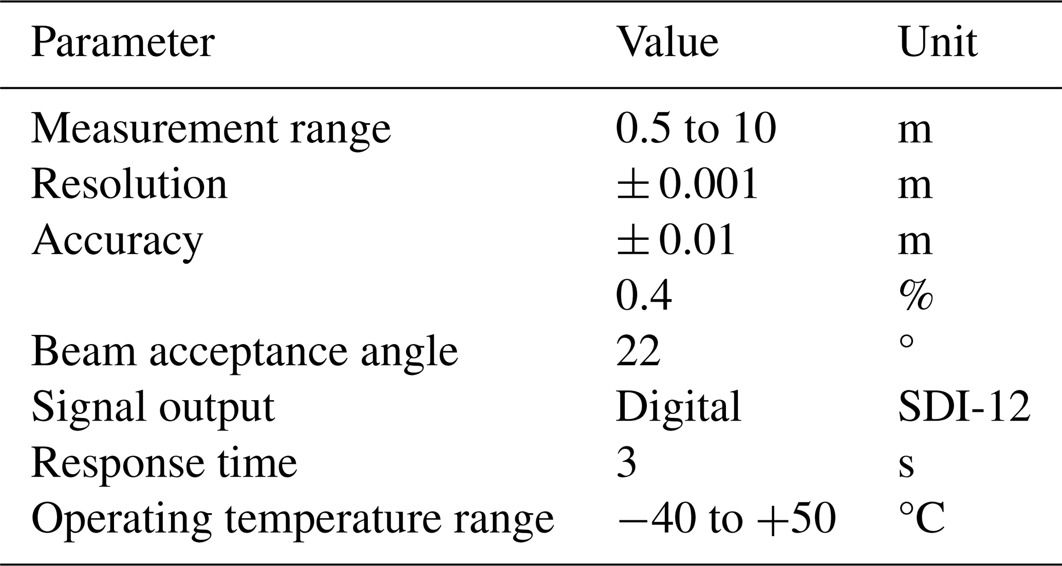
Pressure transducer assembly

The ablation area AWSs are fitted with an Ørum & Jensen NT1400/NT1700 pressure transducer assembly (PTA), which measures changes in ice surface elevation caused by ablation. According to the manufacturer, the sensor has an accuracy of 2.5 cm. See Fig. A1 for further details on how the system is built.

Figure A1 Schematic of the pressure tranducer assembly.

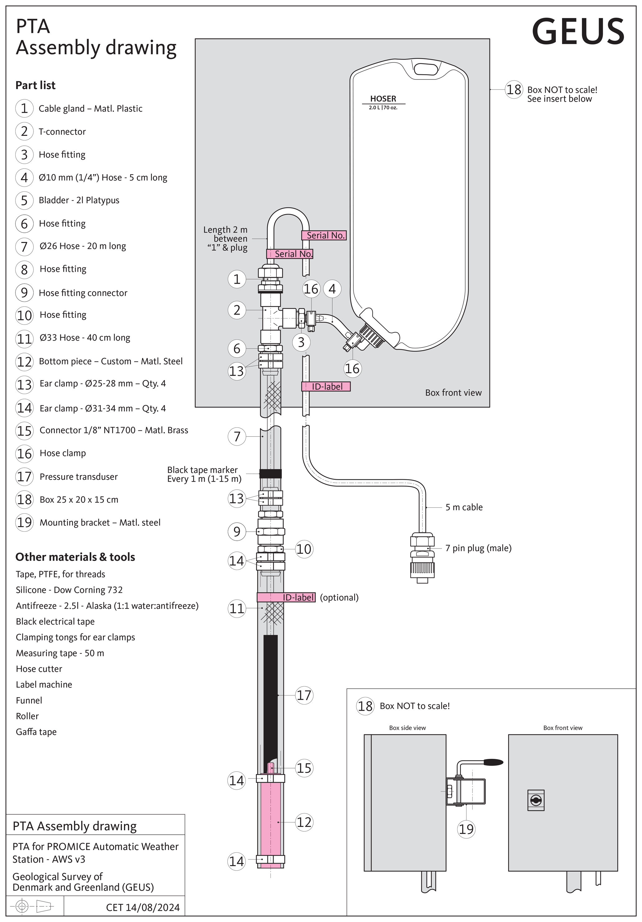
Thermistor Strings

There are four types of thermistor strings deployed: PROMICE (8 sensors) or GC-Net (10 sensors) type, which can be either analogue or digital.

Table A14 RS Pro 100 kΩ NTC thermistor (2.4 × 63.5 mm), a resin-coated negative-temperature-coefficient sensor used for temperature measurement, control, and compensation. The device provides a nominal resistance of 100 kΩ at 25 °C, has a thermal time constant of approximately 10 s, and operates over a temperature range from −80 to +150 °C. It includes 0.2 mm bare tinned lead wires and exhibits stable resistance–temperature behaviour suitable for detecting temperature-induced changes in resistance.

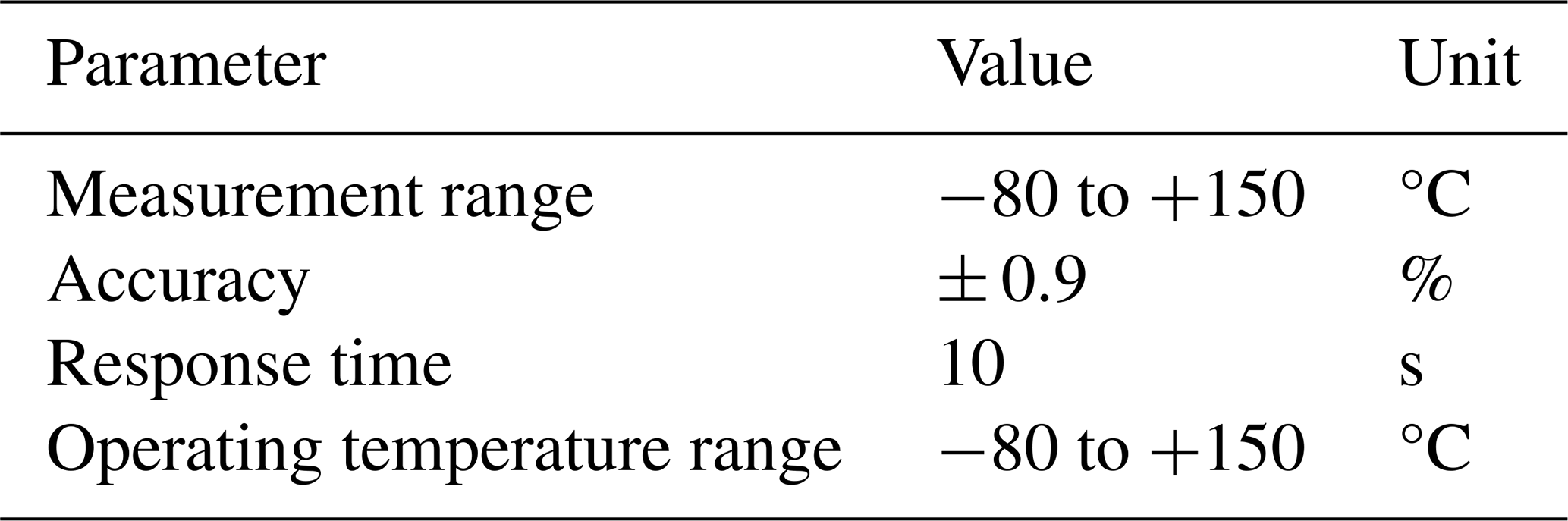
Table A15 GeoPrecision TNode digital thermistor used in multipoint thermistor strings for high-resolution environmental temperature monitoring. The TNode incorporates a digital sensing chip with 0.01 °C resolution and ±0.1 °C base accuracy, and supports up to 48 sensors along a 100 m string. The system is designed for field applications requiring precise temperature profiling in soil, permafrost, wetland, ice, and snow environments.

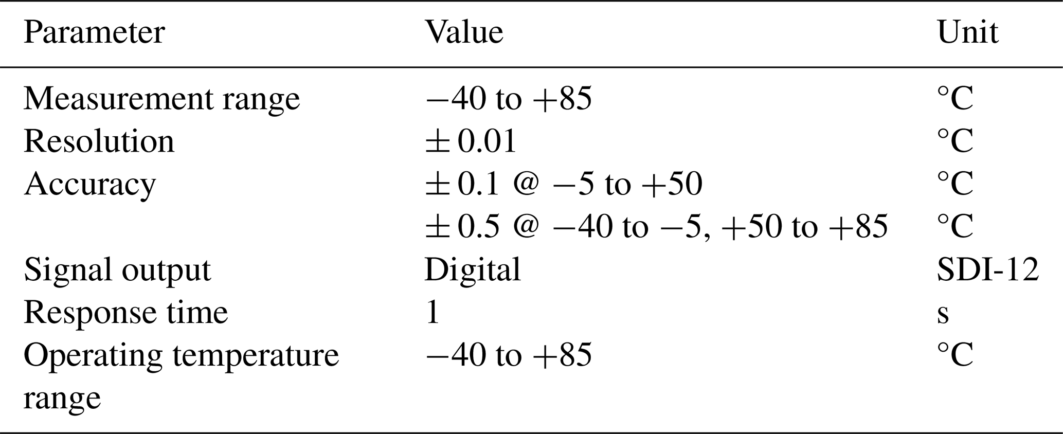
Inclinometers

Table A16 Manufacturer-specific documentation for HL Planartechnik NS-25/E2 (dual axis) inclinometer, which is used as inclinometer for our older version of AWSs.

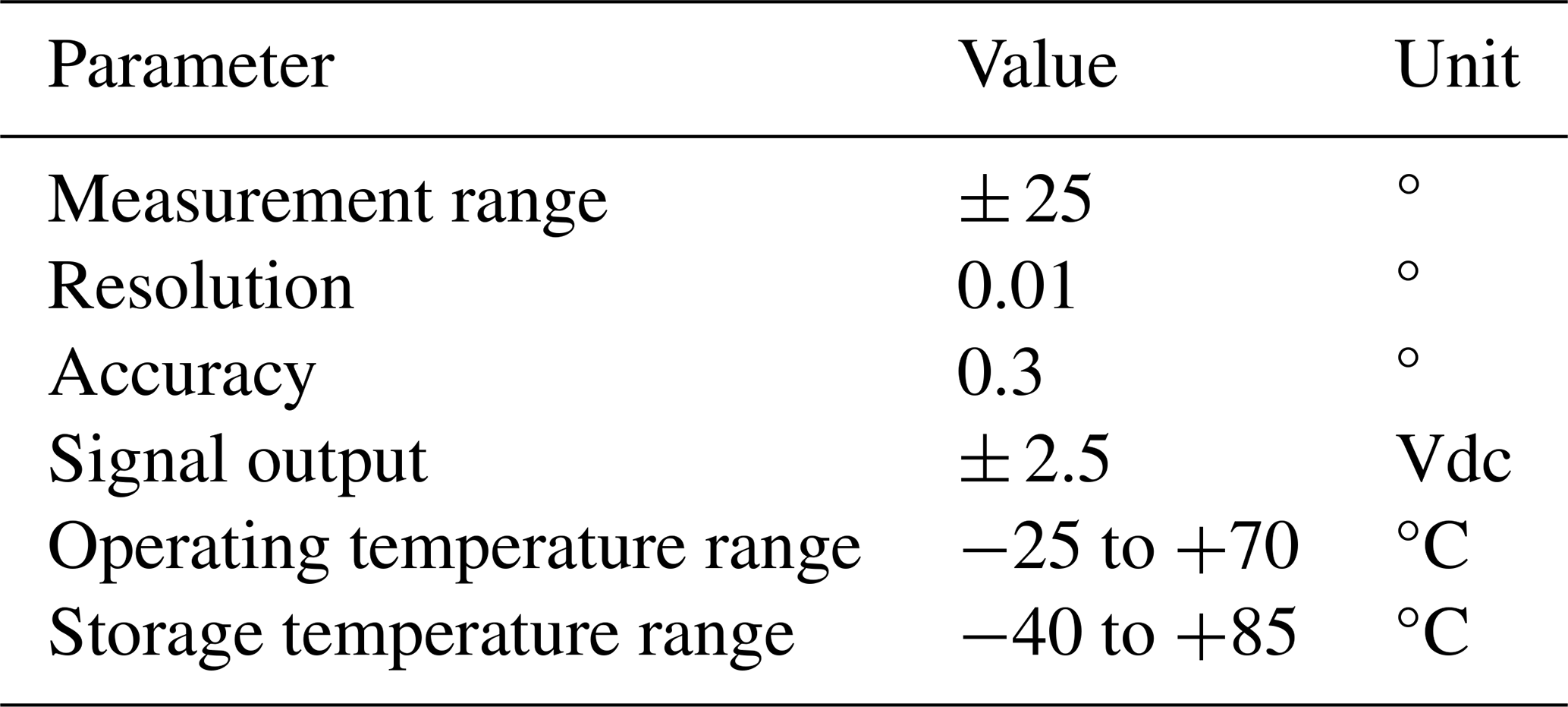
Table A17 Manufacturer-specific documentation for Rion DCM260B (compass/inclinometer), which is used as compass/inclinomter for our newer version of AWSs.

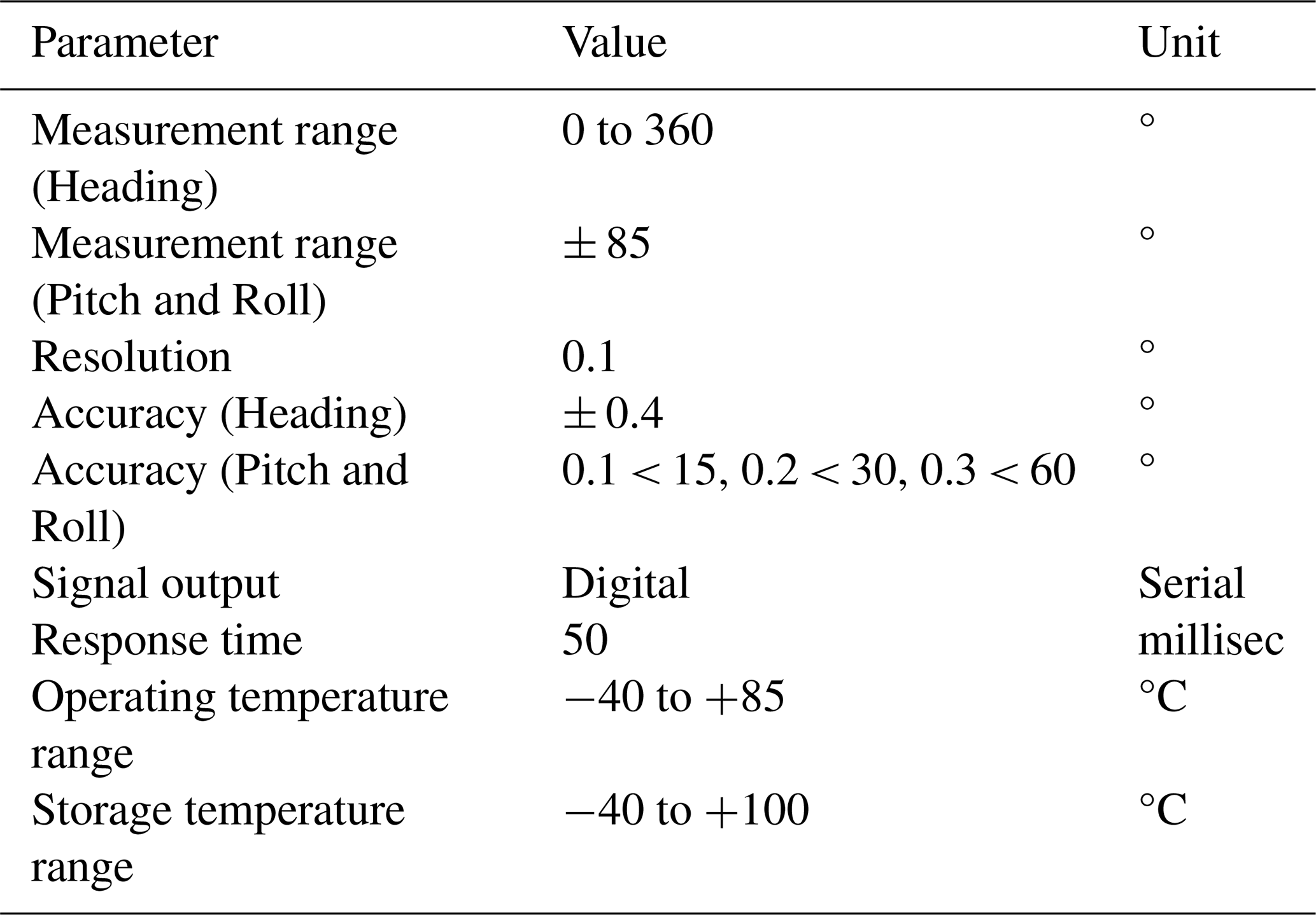
GNSS Antennae

Table A18 Manufacturer-specific documentation for Trimble/NAL SAF5270G: An older external antenna (housed within the loggerbox) is used with the NAL 9602-LP Iridium modem, which houses an L1 GPS.

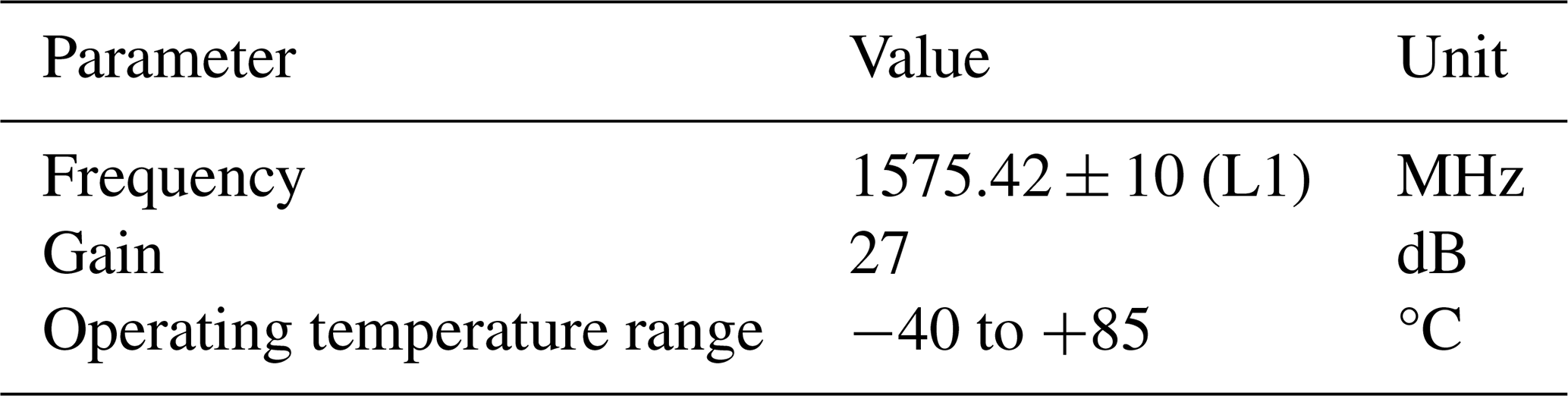
Table A19 Manufacturer-specific documentation for Calian TW4020: A newer external antenna (housed within the loggerbox) is used with the NAL 9602-LP Iridium modem, which houses an L1 GPS.

Appendix B: Data product

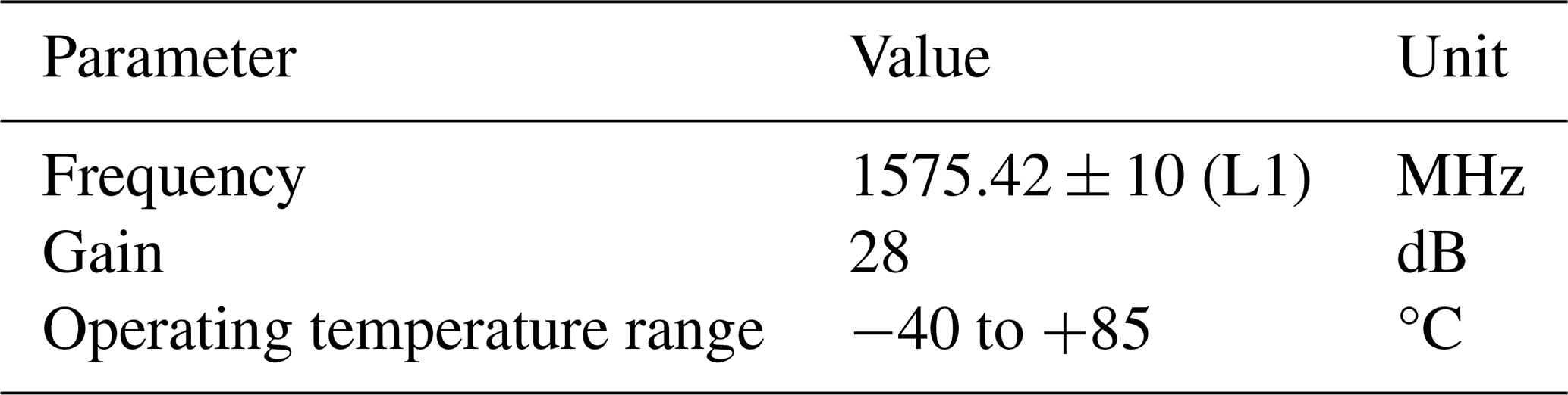
Unrealistic spikes in the data are removed by applying predefined upper and lower thresholds to each measurement. Threshold values used in the filtering process for each measured variable are shown in the Table B1.

Table B1 Threshold values used in the filtering process for each measured variable.

Appendix C: Code availability

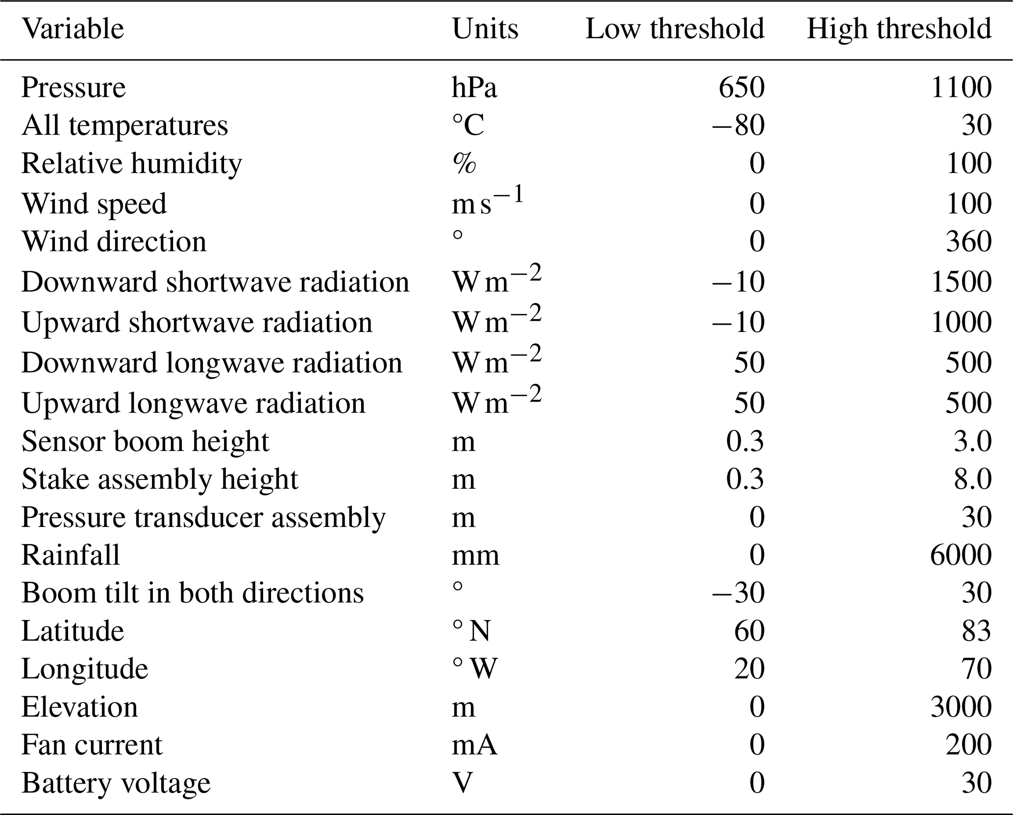
The pypromice production pipeline is available for use and contributions at https://github.com/GEUS-Glaciology-and-Climate/pypromice (last access: 12 November 2025), with a citeable DOI How et al. (2023a) (https://doi.org/10.22008/FK2/3TSBF0) alongside its corresponding, peer-reviewed software publication How et al. (2023b).