A dataset on the structural diversity of European forests

Forest structural diversity, defined as the heterogeneity of canopy structural elements in space, is an important axis of functional diversity and is central to understanding the relationship between canopy structure, biodiversity, and ecosystem functioning. Despite the recognised importance of forest structural diversity, the development of specific data products has been hindered by the challenges associated with collecting information on forest structure over large spatial scales. However, the advent of novel spaceborne LiDAR sensors like the Global Ecosystem Dynamics Investigation (GEDI) is now revolutionising the assessment of forest structural diversity by providing high-quality information on forest structural parameters with a quasi-global coverage. Whilst the availability of GEDI data and the computational capacity to handle large datasets have opened up new opportunities for mapping structural diversity, GEDI only collects sparse measurements of vegetation structure. Continuous information of forest structural diversity over large spatial domains may be needed for a variety of applications. The aim of this study was to create wall-to-wall maps of canopy structural diversity in European forests using a predictive modelling framework based on machine learning. We leverage multispectral and Synthetic Aperture Radar (SAR) data to create a series of input features that were related to eight different structural diversity metrics, calculated using GEDI. The models proved to be robust, indicating that active radar and passive optical data can effectively be used to predict structural diversity. Our dataset (https://doi.org/10.6084/m9.figshare.26058868.v1, Girardello et al., 2024) finds applications in a range of disciplines, including ecology, hydrology, and climate science. As our models can be regularly rerun as new images become available, it can be used to monitor the impacts of climate change and land use management on forest structural diversity.

1 Introduction

Information on forest canopy structure is important for several disciplines, including Earth System Science, Ecology, Hydrology, and Climate Science. Forest canopy structure plays a fundamental role in ecosystem functioning by affecting carbon storage and cycling, regulating the hydrological cycle, and influencing local and regional climate patterns (Migliavacca et al., 2021; Shugart et al., 2010; Sun et al., 2018). In addition, canopy structure is critical for maintaining high levels of biodiversity by supporting a high diversity of ecological niches (LaRue et al., 2019).

The concept of structural diversity or complexity, herein defined as the heterogeneity or variability of canopy structural elements in vertical or horizontal space (Ehbrecht et al., 2021; Hakkenberg et al., 2023; LaRue et al., 2019), is central to understanding the relationship between canopy structure, biodiversity, and ecosystem functioning. Structurally diverse forests can host a wide variety of functionally complementary species, which tend to increase resource-use efficiency and promote feedbacks that enhance resource availability (Gough et al., 2019; Murphy et al., 2022). As a result, these forests can capture light more efficiently, leading to increased ecosystem productivity (Atkins et al., 2018; Toda et al., 2023). Therefore, the availability of data on forest structural diversity over large spatial scales is critical for predicting and managing the response of forest ecosystems to global change.

Mapping forest structural diversity over large spatial scales proved challenging due to the lack of comprehensive datasets and consistent data collection methodologies, hindering our ability to predict ecosystem function at large geographic scales. Whilst forest structural parameters can be measured in various ways, traditional field-based measures of stand structure are generally labour-intensive and have been limited to small areas (Goodbody et al., 2023). Laser scanning, or LiDAR, has been proved a sound alternative for measuring tree height from 3D data measured through echoes (Coops et al., 2021). However, data from airborne LiDAR have been limited in spatial and temporal coverage to specific regions (Hancock et al., 2021). Recent advances in satellite remote sensing technology and computational capabilities have made it possible to measure a range of structural variables at larger scales than ever before. Notably, the Global Ecosystem Dynamics Investigation (GEDI) (Dubayah et al., 2020) instrument, placed on board the International Space Station (ISS) in December 2018, collecting LiDAR samples until March 2026, has revolutionized the assessment of forest structure. Recent studies have shown how structural data collected by GEDI can be used in several applications ranging from biomass estimation to the monitoring of biodiversity and ecosystem disturbances (Crockett et al., 2023; Hakkenberg et al., 2023; Holcomb et al., 2024). These early examples demonstrate the future potential of the GEDI mission.

Whilst the availability of GEDI data and the computational capacity to handle large datasets have opened up new opportunities to map structural diversity, GEDI only collects sparse measurements of vegetation structure. Although the GEDI mission has recently been extended, it is expected to cover only a minimal fraction of the land surface. Depending on the application of interest, continuous information on structural diversity over forests may be needed. Combining GEDI with other types of satellite remote sensing data within a machine learning framework may thus be necessary for the creation of structural diversity data products that have continuous coverage and that extend beyond the timeframe covered by the GEDI mission. In this context, predictor variables derived from complementary satellite observations are used to bridge the gap between sparse GEDI measurements and the need for wall-to-wall maps of forest structural diversity. These predictors can act as observable proxies for canopy structural complexity, enabling the spatial extrapolation of the GEDI-derived structural diversity metrics across Europe. Several recent studies have successfully combined GEDI data with other remote sensing data sources to predict canopy structure in areas not covered by GEDI, paving the way for mapping specific structural features of vegetation regionally and globally (Aragoneses et al., 2024; Lang et al., 2023; Potapov et al., 2021; Schwartz et al., 2024). Additionally, preliminary efforts to assess the potential of GEDI data to capture canopy diversity over different regions have been carried out (Schneider et al., 2020). However, despite these significant advances, no efforts have been made to map forest structural diversity at a continental scale in Europe.

To address the lack of readily available structural diversity data, we combined a suite of structural diversity indicators calculated using GEDI data with active radar and passive optical data from the Sentinel-1, Sentinel-2, and ALOS-PALSAR-2 missions. This sensor combination was specifically selected to enable spatially and temporally consistent, wall-to-wall estimates suitable for large-scale and monitoring, while capturing complementary structural information across different canopy layers: Sentinel-2 multispectral data are sensitive to canopy biochemical and structural properties at the crown surface, including vegetation density and phenological state. Sentinel-1 C-band SAR interacts primarily with the upper canopy and smaller structural components, capturing variations in canopy roughness ALOS-PALSAR-2 L-band SAR, owing to its longer wavelength, exhibits enhanced sensitivity to larger structural elements and sub-canopy features, providing information on forest vertical complexity. These different sources of data were then integrated using a predictive modelling framework, based on a machine learning method. The resulting models were used to predict structural diversity across Europe. Although Sentinel-1, Sentinel-2 and ALOS-PALSAR-2 data have been previously used for predicting canopy height and other structural components of forests, their joint use for mapping forest structural diversity has not yet been attempted (Liu et al., 2025; Wang et al., 2024). Our analysis includes a total of eight structural diversity metrics, including metrics that quantify the vertical and horizontal heterogeneity of the canopy, as well as metrics that quantify the heterogeneity of forest structure among GEDI observations within a given area. The dataset presented here is readily available for use as input in various environmental models and analyses.

Table 1 Structural diversity metrics computed in this study.

2 Methods

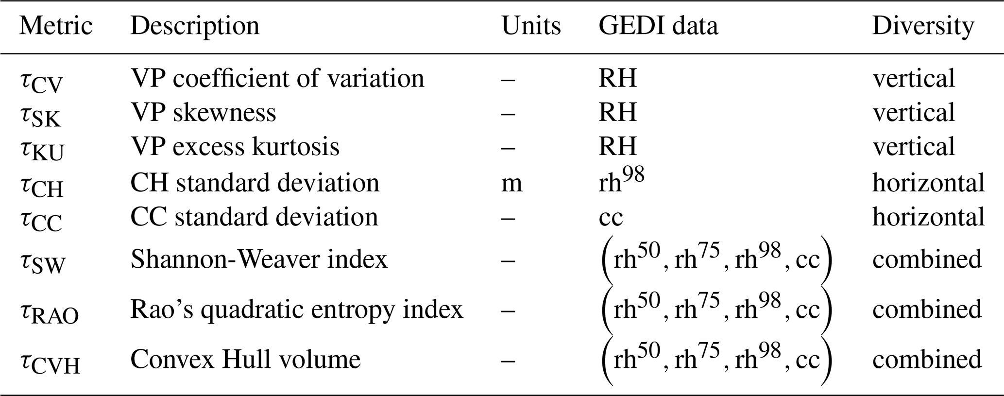
We calculated eight forest structural diversity metrics using NASA GEDI observations (Dubayah et al., 2020). A list of the metrics is reported in Table 1. A machine learning (ML) framework was used to model the relations between each metric and a series of predictors derived from passive optical and active radar remote sensing data. The model was then used to create a structural diversity dataset that covers the whole forested domain of Europe, extending up to ∼ 52° N, which corresponds to the northern latitudinal limit of the GEDI mission. The creation of the dataset involved five main steps (Fig. 1): (i) satellite remote sensing data pre-processing, (ii) structural diversity metric calculation (iii) model training, (iv) model validation, and (v) prediction (Fig. 1). Data from GEDI, Sentinel 1 and 2, ALOS-PALSAR-2 were pre-processed and downloaded from Google Earth Engine (GEE), a cloud-based infrastructure that combines a multi-petabyte catalogue of satellite imagery and geospatial datasets with planetary-scale analysis capabilities (Gorelick et al., 2017).

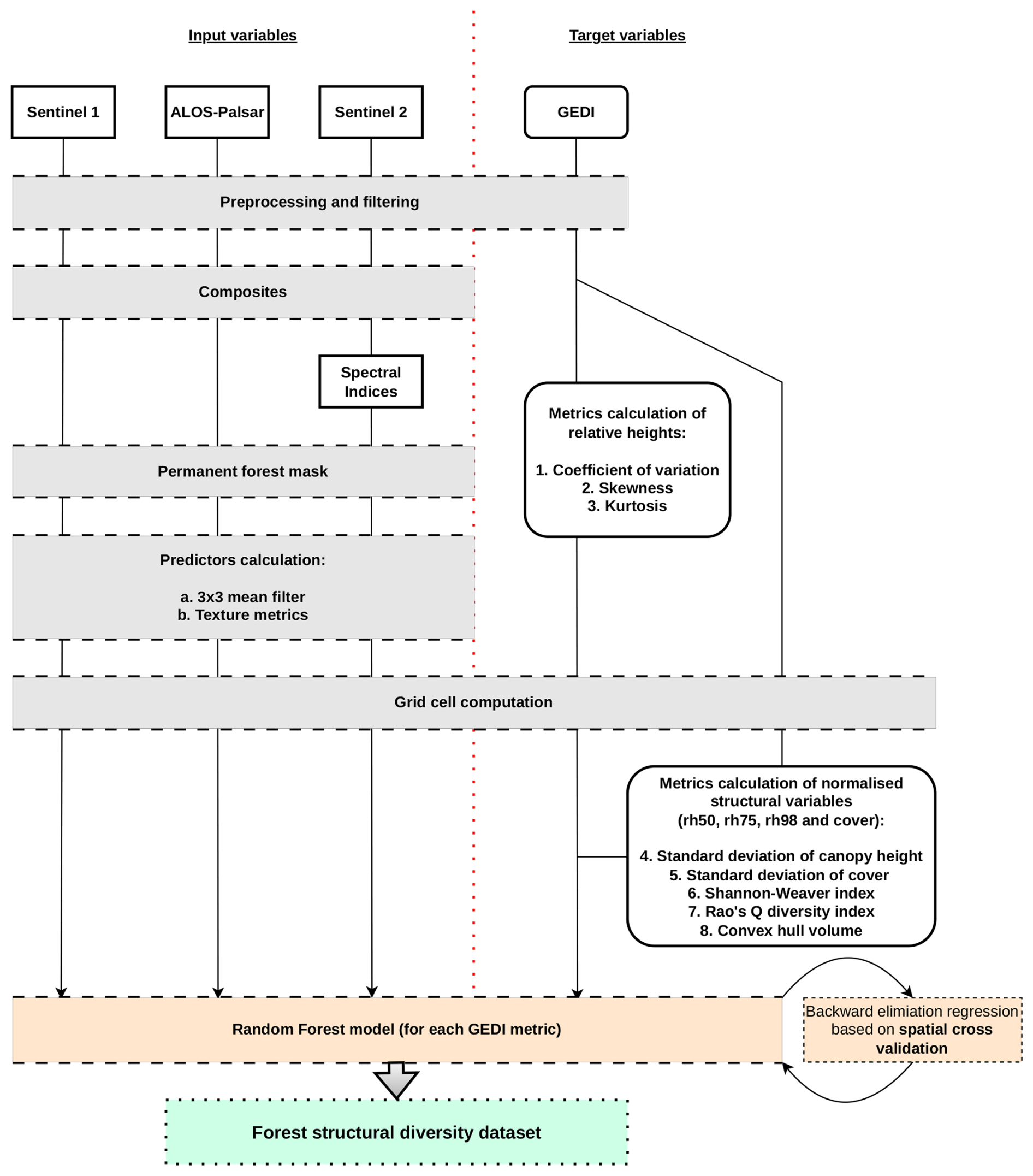
Figure 1 General workflow employed in the creation of the forest structural diversity dataset. The workflow is segmented by a red dashed line, delineating the Remote Sensing predictors from the inputs to the target GEDI data. Boxes with solid edges represent the data that were directly utilised to train the Random Forest models. The grey boxes indicate the preliminary steps undertaken before the model training phase. The process culminates with orange boxes, which signifies the development of the predictive model itself, leading to the green box that represents the final output outcome – the forest structural diversity dataset.

We used data covering forests that had remained ecologically stable, meaning they experienced no canopy loss, from 2000 to 2021, as identified through the Global Forest Change product by Hansen et al. (2013). Furthermore, our analyses were limited to areas where tree cover exceeded 30 % and which bordered at least 6 out of 8 neighbouring pixels, also with tree cover exceeding 30 %. While our threshold is more stringent than Food and Agriculture Organization (FAO) definition of forest (FAO, 2000), which specifies an area spanning more than 0.5 hectares with trees taller than 5 m and a canopy cover of more than 10 %, it was chosen to capture areas with substantial arboreal density. Although our selection was guided by the FAO's broader forest criteria, we customized these guidelines to suit our research focus. This threshold was intentionally adopted to focus on landscapes with well-developed and spatially continuous forest canopies. This more conservative threshold reduces the influence of sparsely treed or transitional land-cover types and improves the robustness and interpretability of GEDI-based structural diversity metrics

2.1 Structural diversity metrics

Structural diversity can be characterized in a variety of ways depending on the data from which it is calculated and the intended application. In this work we adopted the common definition where diversity is defined in the vertical dimension as heterogeneity of vegetation height and in the horizontal dimension as canopy heterogeneity (Hakkenberg and Goetz, 2021). We chose a set of metrics that would characterize the heterogeneity within and among structural features for a given area, reflecting both local (alpha) and regional (beta) measures of structural diversity. These complementary metrics have been demonstrated to be particularly crucial for predicting tree diversity and ecosystem functioning (Coverdale and Davies, 2023; Ma et al., 2022; Zhai et al., 2024). A summary of the metrics with the input data used is reported in Table 1. Several GEDI products, including Foliage Height Diversity (FHD from the GEDI L2B product) and the Waveform Structural Complexity Index (WSCI, from the GEDI L4C product), already capture important aspects of forest structural heterogeneity and have proven highly valuable for large-scale analyses. However, recent work has shown that these indices exhibit strong scaling relationships with top-of-canopy height (RH98) (de Conto et al., 2024).

In the context of this study, our objective was therefore not to directly use existing GEDI products as target variables, but to develop structural diversity metrics that explicitly quantify heterogeneity while minimising direct dependence on canopy height. This motivated the selection of eight complementary metrics based on the distributional properties of GEDI relative height profiles and canopy cover, ecologically interpretable, minimally redundant with each other and with height, and suitable for spatial aggregation and wall-to-wall mapping using multi-sensor satellite data.

The eight structural diversity metrics were designed to span three complementary dimensions of forest structural diversity (Table 1). Vertical heterogeneity within individual canopy profiles is characterised using distributional metrics derived from GEDI relative height profiles, namely the coefficient of variation, skewness, and kurtosis, which capture differences in vertical layering and profile shape. Horizontal heterogeneity is described by the variability among GEDI observations within a spatial unit, quantified through the standard deviation of canopy height (CH) and canopy cover (CC), reflecting spatial variation in canopy structure across the landscape. Finally, combined structural diversity is represented using multivariate metrics (Shannon index (SW), Rao's quadratic entropy (RAO), and convex hull volume (CVH)), which synthesize information from multiple GEDI measurements into a single integrated index per spatial unit. Together, these metrics provide an interpretable yet comprehensive characterisation of forest structural diversity while minimising redundancy among metrics and with top-of-canopy height.

2.1.1 GEDI input data and general framework

GEDI data are collected from a full waveform LiDAR sensor operating onboard the International Space Station (ISS) from April 2019 until March 2026. Due to the orbital path of the International Space Station (ISS), GEDI's coverage is primarily limited to latitudes between ∼ 50° N and S. The instrument provides sparse measurements (hereinafter sample plots or shots) of vegetation structure over an area defined by a sampling footprint of about 25 m diameter.

Input data included the GEDI Level 2A Relative Heights (RH), and the Level 2B total Canopy Cover (CC) values (see Table 1). In the literature, rh⁹⁸ is taken as a reference for the top canopy height (CH) (Lang et al. 2023), CC is the proportion of the shot covered by the vertical projection of the tree crowns. The GEDI data were downloaded from GEE after applying a filtering procedure to remove low-quality and unreliable observations and to reduce noise in the input data, based on standard GEDI quality flags and thresholds (Table S1 in the Supplement).

Structural diversity metrics were computed for each spatial analysis unit, defined as regular grid cells (hereafter referred to pixels) at 1, 5, and 10 km spatial resolution. For each pixel, all number (M) of valid GEDI shots overlapping the pixel between April 2019 and January 2023 were collected. The structural diversity metrics of a given pixel are calculated by aggregating all M overlapping that pixel. Each GEDI shot i was characterized by its RH distribution ${\mathrm{rh}}_i=\left\{{\mathrm{rh}}_i^k,{\mathrm{rh}}_i^{k+\mathrm{1}},\mathrm{\dots },{\mathrm{rh}}_i^{\mathrm{100}}\right\}$ with k: ${\mathrm{rh}}_i^k\ge \mathrm{0}$ (i.e. only the positive values were considered) and total canopy cover cc_i. To ensure robust estimation of structural diversity, pixels with fewer GEDI observations than a minimum sampling threshold were excluded. This threshold was defined as the median number of valid GEDI shots across all pixels at a given spatial resolution. In addition, extreme metric values were filtered using a z-score criterion, with values exhibiting a deviation greater than 3 across pixels discarded as outliers. The remaining pixels were then used to compute the structural diversity metrics. A post-processing step was applied to remove extreme values: pixels with structural diversity values exhibiting a z-score greater than 3 were discarded as outliers.

We computed the eight structural diversity metrics at three spatial resolutions (1, 5, and 10 km) using grids in the Lambert Azimuthal Equal Area (LAEA) projection. The choice of these spatial resolutions reflects a trade-off between spatial detail, GEDI sampling density, and metric robustness. Because GEDI provides sparse footprint-level measurements, reliable estimation of structural diversity requires a sufficient number of observations within each spatial unit. Coarser resolutions improve metric stability, while finer resolutions provide greater spatial detail at the cost of higher uncertainty. The 10 km resolution was identified as the most robust scale for continental-scale analyses and is compatible with the spatial aggregation typically used in regional ecosystem and Earth system models. The 5 and 1 km products support applications requiring finer spatial detail, such as regional ecological analyses and biodiversity assessments. We acknowledge that applications focused on small-scale disturbances, edge effects, or forest fragmentation would benefit from even finer resolution; however, at such scales, the limited density of GEDI observations substantially constrains reliable metric estimation over large areas.

In the following sections, we detail the methodology employed for calculating the diversity metrics and predictor variables, which makes use of the mean μ(X), standard deviation σ(X), skewness γ(X), excess kurtosis κ(X), coefficient of variation cv(X) of a variable $X=\left\{x_{\mathrm{1}},\mathrm{\dots },x_M\right\}$, where X represents a vector of observations (see Appendix A for the explicit formulations).

2.1.2 Vertical Diversity Metrics

RH metrics provide information on the vertical distribution of the plant elements, that is, the vertical profile (VP) of the vegetation (see Fig. S1 in the Supplement). The VP in a sample can be reconstructed from the corresponding RH distribution, and the profile's moments (i.e. mean, standard deviation, skewness, kurtosis) are well approximated by the RH distribution's moments (Fig. S1 in the Supplement).

The following calculated indicators characterise the heterogeneity of the vertical profile:

1. the average coefficient of variation of the vertical profiles

   $$\begin{array}{}\text{(1)}& {\mathit{\tau }}_{\mathrm{CV}}=\mathit{\mu }\left(\mathrm{CV}\right)\end{array}$$

   with $\mathrm{CV}=\left\{\mathrm{cv}\left({\mathrm{rh}}_{\mathrm{1}}\right),\mathrm{\dots },\mathrm{cv}\left({\mathrm{rh}}_M\right)\right\}$. The coefficient of variation cv(RH)quantifies the extent of vertical variability in relation within a vertical profile as the ratio between the standard deviation and the mean of the relative height distribution. τ_CV therefore indicates greater vertical dispersion relative to mean profile height and hence greater vertical heterogeneity;

2. the average skewness of the vertical profiles

   $$\begin{array}{}\text{(2)}& {\mathit{\tau }}_{\mathrm{SK}}=\mathit{\mu }\left(\mathrm{\Gamma }\right)\end{array}$$

   where $\mathrm{\Gamma }=\left\{\mathit{\gamma }\left({\mathrm{rh}}_{\mathrm{1}}\right),\mathrm{\dots },\mathit{\gamma }\left({\mathrm{rh}}_M\right)\right\}$ represents the set of skewness values computed from the RH distribution of each of the M GEDI observations within the pixel. Skewness γ(RH), or third standardized moment, is a measure of the asymmetry of the VP about its mean, and it can be positive, negative, or zero (Fig. S2a and d in the Supplement). If VP is a unimodal distribution (a distribution with a single peak), positive skewness generally indicates an asymmetric tail extending toward larger height values (overstorey heterogeneity), while negative skewness suggests a tail extending toward smaller height values (understorey heterogeneity). However, note that in the cases where one tail is long, but the other tail is fat, or the distribution is multi-modal, skewness does not always obey this simple rule.

3. the average excess kurtosis of the vertical profiles

   $$\begin{array}{}\text{(3)}& {\mathit{\tau }}_{\mathrm{KU}}=\mathit{\mu }\left(K\right)\end{array}$$

   where $K=\left\{\mathit{\kappa }\left({\mathrm{rh}}_{\mathrm{1}}\right),\mathrm{\dots },\mathit{\kappa }\left({\mathrm{rh}}_M\right)\right\}$ represents the set of excess kurtosis values computed from the RH distribution of each of the M GEDI observations within the pixel Excess κ(RH) is a measure of the “tailedness” of the VP, and it is equal to 0 for any univariate normal distribution, (Fig. S2a and d in the Supplement). Distributions with negative/positive excess kurtosis are said to be platykurtic/leptokurtic. Platykurtic distributions show fewer and/or less extreme outliers than the normal distribution. In this case, the vegetation mass is more concentrated around the VP mean than near the vertical extremes (i.e. the ground and to top canopy height). However, it is important to note that while kurtosis, the fourth moment, does play a role in characterizing the shape of VP, its influence is comparatively smaller than that of the standard deviation, the second moment, and skewness, the third moment. For instance, two distinct VPs may exhibit identical excess kurtosis while displaying markedly disparate distributions in terms of standard deviations.

2.1.3 Horizontal Diversity Metrics

We calculated 5 vertical horizontal diversity indices.

1. the standard deviation of the canopy heights

   $$\begin{array}{}\text{(4)}& {\mathit{\tau }}_{\mathrm{CH}}=\mathit{\sigma }\left(\mathrm{CH}\right)\end{array}$$

   where $\mathrm{CH}=\left\{{\mathrm{rh}}_{\mathrm{1}}^{\mathrm{98}},\mathrm{\dots },{\mathrm{rh}}_M^{\mathrm{98}}\right\}$ represents the set of rh⁹⁸values within the τ_CHτ_CH indicates the spread of the canopy heights in the area.

2. the standard deviation of the total canopy cover

   $$\begin{array}{}\text{(5)}& {\mathit{\tau }}_{\mathrm{CC}}=\mathit{\sigma }\left(\mathrm{CC}\right)\end{array}$$

   where $\mathrm{CC}=\left\{{\mathrm{cc}}_{\mathrm{1}},\mathrm{\dots },{\mathrm{cc}}_M\right\}$ represents the set of canopy cover values within the pixel. τ_CC indicates the spread of the total canopy cover in the area.

2.1.4 Combined Vertical and Horizontal and Diversity Metrics

• 3.

  the Shannon-Weaver index

  $$\begin{array}{}\text{(6)}& {\mathit{\tau }}_{\mathrm{SW}}=-\sum _{\log p_{\mathit{\epsilon }\mathit{\pi }o\mathit{\omega }}}{p}_{\mathit{\epsilon }\mathit{\pi }o\mathit{\omega }}\log p_{\mathit{\epsilon }\mathit{\pi }o\mathit{\omega }}\end{array}$$

  in a 4D cartesian space defined on the basis $\left({\mathrm{rh}}^{\mathrm{50}},{\mathrm{rh}}^{\mathrm{75}},{\mathrm{rh}}^{\mathrm{98}},\mathrm{cc}\right)$, where p_επoω is the fraction of the GEDI samples within the pixel falling in a specific bin (see Appendix A2). We used a 5-unit bin size on each axis, and the GEDI CC values were amplified by 10. τ_SW measures the uncertainty or disorder inherent to the variable's possible outcomes. τ_SW=0 when all observations are confined within a single bin, otherwise τ_SWis larger than zero. Higher values indicate heterogeneity, while lower values suggest homogeneity.

• 4.

  Rao's quadratic diversity index

  $$\begin{array}{}\text{(7)}& {\mathit{\tau }}_{\mathrm{RAO}}={\sum }_{\mathit{\epsilon }\mathit{\pi }o\mathit{\omega }}{\sum }_{{\mathit{\epsilon }}^{\prime }{\mathit{\pi }}^{\prime }{o}^{\prime }{\mathit{\omega }}^{\prime }}{p}_{\mathit{\epsilon }\mathit{\pi }o\mathit{\omega }}{D}_{\mathit{\epsilon }\mathit{\pi }o\mathit{\omega }}^{{\mathit{\epsilon }}^{\prime }{\mathit{\pi }}^{\prime }{o}^{\prime }{\mathit{\omega }}^{\prime }}{p}_{{\mathit{\epsilon }}^{\prime }{\mathit{\pi }}^{\prime }{o}^{\prime }{\mathit{\omega }}^{\prime }}\end{array}$$

  in the 4D cartesian space defined on the basis $\left({\mathrm{rh}}^{\mathrm{50}},{\mathrm{rh}}^{\mathrm{75}},{\mathrm{rh}}^{\mathrm{98}},\mathrm{cc}\right)$, where p_επoω is the fraction of the GEDI samples within the pixel falling in a specific bin and $D_{\mathit{\epsilon }\mathit{\pi }o\mathit{\omega }}^{{\mathit{\epsilon }}^{\prime }{\mathit{\pi }}^{\prime }{o}^{\prime }{\mathit{\omega }}^{\prime }}$ the cartesian distance between two bins (see Appendix A2). We used a 1-unit bin size on each axis, and the GEDI CC values were amplified by 10. τ_RAO ranges from zero, indicating no diversity, to positive numbers. Differently from τ_SWindex, τ_RAO considers both abundance (p_επoω terms) and dissimilarity in the sampled data ($D_{\mathit{\epsilon }\mathit{\pi }o\mathit{\omega }}^{{\mathit{\epsilon }}^{\prime }{\mathit{\pi }}^{\prime }{o}^{\prime }{\mathit{\omega }}^{\prime }}$ term).

• 5.

  convex hull volume

  $$\begin{array}{}\text{(8)}& {\mathit{\tau }}_{\mathrm{CVH}}=\mathrm{CVH}\left(\mathrm{SHT}\right)\end{array}$$

  in the 4D cartesian space defined on the basis $\left({\mathrm{rh}}^{\mathrm{50}},{\mathrm{rh}}^{\mathrm{75}},{\mathrm{rh}}^{\mathrm{98}},\mathrm{cc}\right)$. We used a 1-unit bin size on each axis, and the GEDI CC values were amplified by 10. CVH is the function calculating the convex hull volume on the ensemble $\mathrm{SHT}=\left\{{\mathrm{sht}}_{\mathrm{1}},\mathrm{\dots },{\mathrm{sht}}_M\right\}$, with ${\mathrm{sht}}_i=\left({\mathrm{rh}}_i^{\mathrm{50}},{\mathrm{rh}}_i^{\mathrm{75}},{\mathrm{rh}}_i^{\mathrm{98}},{\mathrm{cc}}_i\right)$. Larger volumes indicate increased heterogeneity.

2.2 Predictor variables

The variables used as ML predictors were calculated from Sentinel-1, Sentinel-2, and ALOS-PALSAR-2 observed data, which provide complementary information on forest canopy structure derived from optical reflectance, C- and L-band SAR backscatter, and associated textural properties. The predictor calculation involved the following steps:

1. appropriate bands/indices ϕ_α were calculated from the remote sensing raster images;

2. the ${\mathit{\varphi }}_{\mathit{\alpha },i}^{\mathit{\beta }}$ values, with β equal to Spatial Mean (SM), Angular Second Moment (ASM), Entropy (ENT), or Dissimilarity Index (DISS), are calculated from the pixels within the 7 × 7 window aligned with the footprint of the GEDI shot i. ${\mathit{\varphi }}_{\mathit{\alpha },i}^{\mathrm{SM}}$is the spatial mean. ${\mathit{\varphi }}_{\mathit{\alpha },i}^{\mathrm{ASM}}$, ${\mathit{\varphi }}_{\mathit{\alpha },i}^{\mathrm{ENT}}$, and ${\mathit{\varphi }}_{\mathit{\alpha },i}^{\mathrm{DISS}}$ are the texture metrics ASM, ENT, and DISS, respectively (see Appendix A3).

3. the raster images of the predictors were computed as ${\mathit{\varphi }}_{\mathit{\alpha }}^{\mathit{\beta }}=\mathit{\mu }\left({\mathrm{\Phi }}_{\mathit{\alpha }}^{\mathit{\beta }}\right)$, where the mean is calculated on the M values ${\mathrm{\Phi }}_{\mathit{\alpha }}^{\mathit{\beta }}=\left\{{\mathit{\varphi }}_{\mathit{\alpha },\mathrm{1}}^{\mathit{\beta }},\mathrm{\dots },{\mathit{\varphi }}_{\mathit{\alpha },M}^{\mathit{\beta }}\right\}$ corresponding to the geographical positions that overlap the image pixels.

In the following, we present what satellite remote sensing data were used and how they were combined for the calculation of the indices. A total of 47 predictors were derived. A summary of the predictors is reported in Table S2 in the Supplement.

2.2.1 Sentinel-1 radar data

The European Space Agency's (ESA) Sentinel-1 (S1) comprises a constellation of two polar-orbiting satellites, sun-synchronous orbit with a 12 d repeat cycle, which operate day and night a C-band (λ = 5.5 cm) Synthetic Aperture Radar (SAR) to capture data at a spatial resolution of approximately 10 m. The radar enables the acquirement of imagery regardless of the weather, and the C-band frequency is particularly effective in interacting with fine vegetative elements such as leaves and branches (Naidoo et al., 2015). In our study, from Sentinel-1 we utilized both backscatter and coherence data.

Backscatter is the portion of the outgoing radar signal that the target redirects directly back towards the radar antenna. The backscatter characteristics provide crucial insights into the physical properties of forest canopies. For the year 2020, we focused on the signal dual-polarization VV and VH Sentinel-1A (S1A) and Sentinel-1B (S1B) Ground Range Detected (GRD) data, acquired in the Interferometric Wide (IW) swath mode, as it predominantly covers land masses (Kellndorfer et al., 2022). VV(H) is a mode that transmits vertical waves and receives vertical (horizontal) waves to create the SAR image. We selected data from the descending orbit, which has been shown to exhibit fewer correlations with evapotranspiration (ET) (Mueller et al., 2022). Sentinel-1 data used in this study were obtained from GEE, where they had already undergone some pre-processing. Preprocessing steps carried out by the GEE team include applying the orbit file for geocoding, removing GRD border noise and thermal noise, and performing radiometric calibration. We performed a radiometric terrain correction following (Vollrath et al., 2020), as well as the removal of stripes and edges. Following radiometric terrain correction and the removal of stripes and edge artefacts, we selected all valid Sentinel-1 observations captured over Europe within a six-month window centred on the date of maximum NDVI identified independently for each pixel from the Sentinel-2 dataset (see Sect. 2.2.3). We then derived:

1. the S1 backscatter 6-month mean ϕ_S1VVgsμ and ϕ_S1VHgsμ, where the mean is intended to mitigate speckle noise while emphasizing the vegetation growing season;

2. the S1 backscatter standard deviation growing season ϕ_S1VVgsσ and ϕ_S1VHgsσ;

3. the S1 backscatter bi-monthly mean ϕ_S1VVpreμ and ϕ_S1VHpreμ for a window extending 2 months before the month before the peak, ϕ_S1VVactμ and ϕ_S1VHactμ for the period spanning one month before to one month after the peak, and ϕ_S1VVpostμ and ϕ_S1VHpostμ for the two months after the month after the peak.

Coherence is the relationship between waves in a beam of electromagnetic (EM) radiation. Two wave trains of EM radiation are coherent when they are in phase. In radar, the term coherence is also used to describe systems that preserve the phase of the received signal. Coherence measurements serve as a valuable tool for monitoring temporal changes in forested environments (Bruggisser et al., 2021; Cartus et al., 2022). The coherence data utilized in this study were extracted from the dataset developed by Kellndorfer et al. (2022). This dataset is the product of multi-temporal, repeat-pass interferometric processing of S1 SAR images. It incorporates signal dual-polarization VV and VH data from S1A and S1B in Single Look Complex (SLC) format, utilizing the IW swath mode from the year 2020. The product is divided into seasonal sets, and we selected summer (June–August) coherence metrics ϕ_CO, aligned with the growing season, employing a 12 d repeat-pass interval to optimize the balance between image continuity and temporal resolution. This interval was chosen to minimize gaps in the image series, compared to shorter intervals (such as 6 d), while longer intervals (e.g., 18, 24, 36, or 48 d) could result in excessive decorrelation. With a relatively unchanged scene between acquisitions, higher coherence values are achieved, which correlate strongly with the radar signal and hence, reduce noise levels. Furthermore, we prioritized signal VV polarization to enhance our understanding of the data, as it minimizes vegetation decorrelation effects (Pan et al., 2022)

2.2.2 ALOS-PALSAR-2 radar data

The ALOS-PALSAR-2 (Advanced Land Observing Satellite – Phased Array type L-band Synthetic Aperture Radar) system, developed by the Japan Aerospace Exploration Agency (JAXA), operates in the L-band frequency (λ = 23.62 cm) at a spatial resolution of 25 m. The L-band is particularly effective at penetrating canopy layers to provide backscatter signals from larger vegetative features such as branches and trunks, and even from the ground. For our analysis, we made use of the global mosaic of backscatter annual composites, which incorporate signal dual-polarization HH and HV data (Shimada et al., 2014) from the years 2019 and 2020, accessed via GEE. In instances where the data availability was constrained for an annual composite, the dataset was supplemented with observations from adjacent years. To ensure the reliability of our dataset and account for possible gaps in observations, we averaged data across two years to generate ϕ_AP2HHμ and ϕ_AP2HVμ data. This approach helps mitigate noise and stabilize the composite images.

2.2.3 Sentinel-2 optical data

The ESA Sentinel-2 (S2) mission comprises a constellation of two polar-orbiting satellites placed in the same sun-synchronous orbit, phased at 180° to each other. Its high revisit time (10 d at the equator with one satellite, and 5 d with 2 satellites at best) allows monitoring of the Earth's surface changes. The Multi-Spectral Instrument (MSI) on board the 2 platforms collects the sunlight reflected from the Earth and supplies high-resolution multispectral imagery with resolutions of 10 and 20 m. Data are acquired at 10 m spatial resolution for Visible (Blue, Green, Red) and Near-Infra-Red (NIR) bands, and at 20 m spatial resolution for VNIR-Red Edge (RE1, RE2, RE3, RE4) and Short Wave Infra-Red (SWIR) bands (SWIR1, SWIR2). The Level-2A product provides atmospherically corrected Surface Reflectance (SR) images. In this study we used all the Level-2A images from 2000 to 2021 identified by a scene-level cloud and snow cover smaller than 70 % and 5 %, respectively, as provided by GEE. We then calculated:

1. the Normalized Difference Vegetation Index

   $$\begin{array}{}\text{(9)}& {\mathit{\varphi }}_{\mathrm{NDVI}}={\displaystyle \frac{\mathit{\rho }\mathrm{NIR}-\mathit{\rho }\mathrm{Red}}{\mathit{\rho }\mathrm{NIR}+\mathit{\rho }\mathrm{Red}}}\end{array}$$

   as proposed by Rouse et al. (1974) it is a widely recognized index strongly correlated with vegetation health and primary productivity;

2. the Normalized Difference Water Index

   $$\begin{array}{}\text{(10)}& {\mathit{\varphi }}_{\mathrm{NDWI}}={\displaystyle \frac{\mathit{\rho }\mathrm{NIR}-\mathit{\rho }\mathrm{SWIR}\mathrm{1}}{\mathit{\rho }\mathrm{NIR}+\mathit{\rho }\mathrm{SWIR}\mathrm{1}}}\end{array}$$

   as proposed by Gao (1996), it is correlated with leaf water content.

3. the Normalized Difference Red Edge Index

   $$\begin{array}{}\text{(11)}& {\mathit{\varphi }}_{\mathrm{NDRE}}={\displaystyle \frac{\mathit{\rho }\mathrm{NIR}-\mathit{\rho }\mathrm{RE}\mathrm{1}}{\mathit{\rho }\mathrm{NIR}+\mathit{\rho }\mathrm{RE}\mathrm{1}}}\end{array}$$

   as proposed by Gitelson and Merzlyak (1994) it offers sensitivity to chlorophyll content and is useful in assessing forest composition and canopy cover;

4. the Modified Soil Adjusted Vegetation Index

   $$\begin{array}{}\text{(12)}& {\mathit{\varphi }}_{\mathrm{MSAVI}}={\displaystyle \frac{\mathrm{2}\cdot \mathit{\rho }\mathrm{NIR}+\mathrm{1}-\sqrt{\begin{array}{c}{\left(\mathrm{2}\cdot \mathit{\rho }\mathrm{NIR}+\mathrm{1}\right)}^{\mathrm{2}}-\\ \mathrm{8}\cdot \left(\mathit{\rho }\mathrm{NIR}-\mathit{\rho }\mathrm{Red}\right)\end{array}}}{\mathrm{2}}}\end{array}$$

   as proposed by Qi et al. (1994), it is suited to monitoring vegetation density and dynamics, particularly during early growth stages when bare soil is prevalent, thereby minimizing soil background effects;

5. the Green Normalized Difference Vegetation Index

   $$\begin{array}{}\text{(13)}& {\mathit{\varphi }}_{\mathrm{GNDVI}}={\displaystyle \frac{\mathit{\rho }\mathrm{NIR}-\mathit{\rho }\mathrm{Green}}{\mathit{\rho }\mathrm{NIR}+\mathit{\rho }\mathrm{Green}}}\end{array}$$

   as proposed by Gitelson and Merzlyak (1998), it responds to chlorophyll concentration and is indicative of vegetation composition, structure, habitat conditions, and species diversity;

6. the standard deviation of NDVI

   $$\begin{array}{}\text{(14)}& {\mathit{\varphi }}_{\mathrm{NDVI}\mathit{\sigma }}=\mathit{\sigma }\left(\mathit{\varphi }\mathrm{NDVI}\right)\end{array}$$

   as noted by Perrone et al. (2024), it accounts for a significant portion of the variability observed in-situ plant diversity.

2.3 Model training and validation

We used a machine learning method – Random Forest (Breiman, 2001) – to quantify the relations between the remote sensing predictors and the eight metrics. Random Forest is an ensemble learning method based on decision trees that is widely employed for regression tasks. A key advantage of Random Forests is that model fitting is relatively fast and hyperparameter optimization requires only a moderate amount of tuning, compared to other machine learning methods. Optimization of the Random Forest model typically involves tuning a number of hyperparameters. These include the size of the forest (i.e. the number of decision trees), the method of bootstrapping samples, and the setting of the maximum depth for the trees. We specified a fixed number of trees, 600; bootstrapping, a technique that involves random sampling with replacement, which contributes to the diversity of the decision trees in the model and helps prevent overfitting; and we did not impose any limitations on the depth of the individual decision trees, allowing them to expand fully. To evaluate the performance of the Random Forest model, we used mean squared error (MSE) as the metric.

To mitigate the potential for overfitting, we used a backward stepwise selection process that begins with a full model including all available predictors. The algorithm then iteratively removes the least important feature, as determined by its contribution to model performance. The relative importance of predictors was assessed using a permutation procedure (Altmann et al., 2010). At each iteration, the model complexity is reduced by one predictor, and the resulting model is evaluated. We compared each newly simplified model to the immediate predecessor to determine whether there was an improvement in performance or a decrease that was less than 1 % worse. The elimination process is halted if the removal of additional predictors causes the model's performance to decrease by more than 1 % compared to the previous iteration. At each step, a spatial cross-validation procedure is used to assess the performance of the model. The metric we utilized to assess model performance throughout this process was the coefficient of determination (R²).

To validate the reduced models, we used two types of validation techniques to assess their predictive accuracy and robustness:

• Random train-validation split: in this approach, the dataset was randomly split, allocating 33 % for model validation. Random validation is a common method that provides a quick and often effective means of evaluating model performance on unseen data. However, it has a notable drawback when dealing with spatial data: it disregards the spatial structure inherent in the dataset (i.e. points close to each other are, generally, more similar than points further away). By ignoring this spatial autocorrelation, random validation may inadvertently conceal overfitting issues, leading to an overly optimistic perception of the model's predictive capabilities.

• 10-Fold Spatial Cross-Validation (Roberts et al., 2016): we implemented a 10-fold spatial cross-validation procedure to address the shortcomings of random validation, thus reducing the overfitting. This more sophisticated method partitions the data into ten spatially distinct subsets, or folds, ensuring that each fold comprises disjointed sets that are geographically separated. The partitioning is achieved by clustering data points according to their spatial coordinates, which preserves the spatial structure and autocorrelation present in the dataset. During the validation process, each fold is used once as a validation set while the remaining folds serve as the training set. This technique provides a more realistic evaluation of the model's performance and its ability to generalize across different spatial regions, thereby offering a safeguard against overfitting and ensuring a more reliable assessment of the model's true predictive power.

Both validation approaches were retained because they address complementary evaluation objectives. Spatial cross-validation provides a conservative assessment of model generalisation in the presence of spatial autocorrelation and is therefore more appropriate for evaluating transferability across regions. Random validation, while potentially optimistic for spatial data, was included to facilitate comparison with previous studies that rely on this approach and to characterise overall model behaviour under standard machine-learning evaluation settings. Throughout the manuscript, spatial cross-validation results are emphasised when discussing model robustness and applicability.

Models were fitted to datasets created at different resolutions including data calculated at 10, 5 and 1 km. Prediction uncertainty was quantified by calculating the standard deviation of predictions across the ensembles of decision trees in the Random Forest models. This metric captures the variability in predictions among individual trees within each model, providing a measure of uncertainty associated with predictions for the different response variables.

3 Results

3.1 Spatial patterns of forest structural diversity

The dataset includes spatial grids for eight structural diversity metrics at three different resolutions (10, 5 and 1 km).

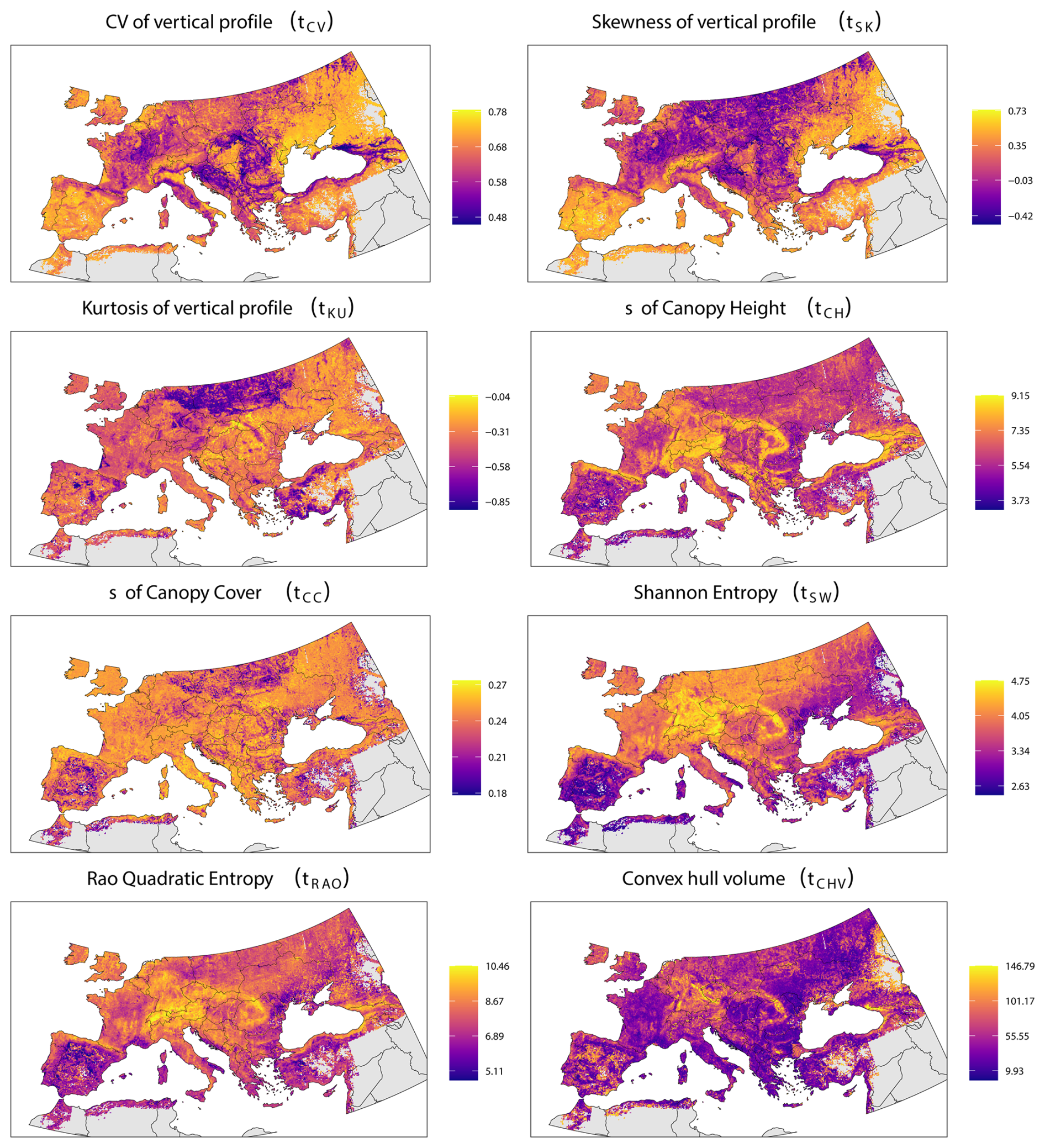
Figure 2 Mapped structural diversity at a 10 km resolution, derived from the Random Forest modelling. Each panel illustrates the geographic distribution of a specific metric (see methods for metric details). The colour palette transitions from purple to yellow, denote an increasing gradient of structural diversity, with warmer colours signifying higher values.

These metrics show a significant variation in structural diversity across the European forests as shown in Fig. 2 (see also Figs. S3 and S4 in the Supplement for 5 and 1 km resolution datasets).

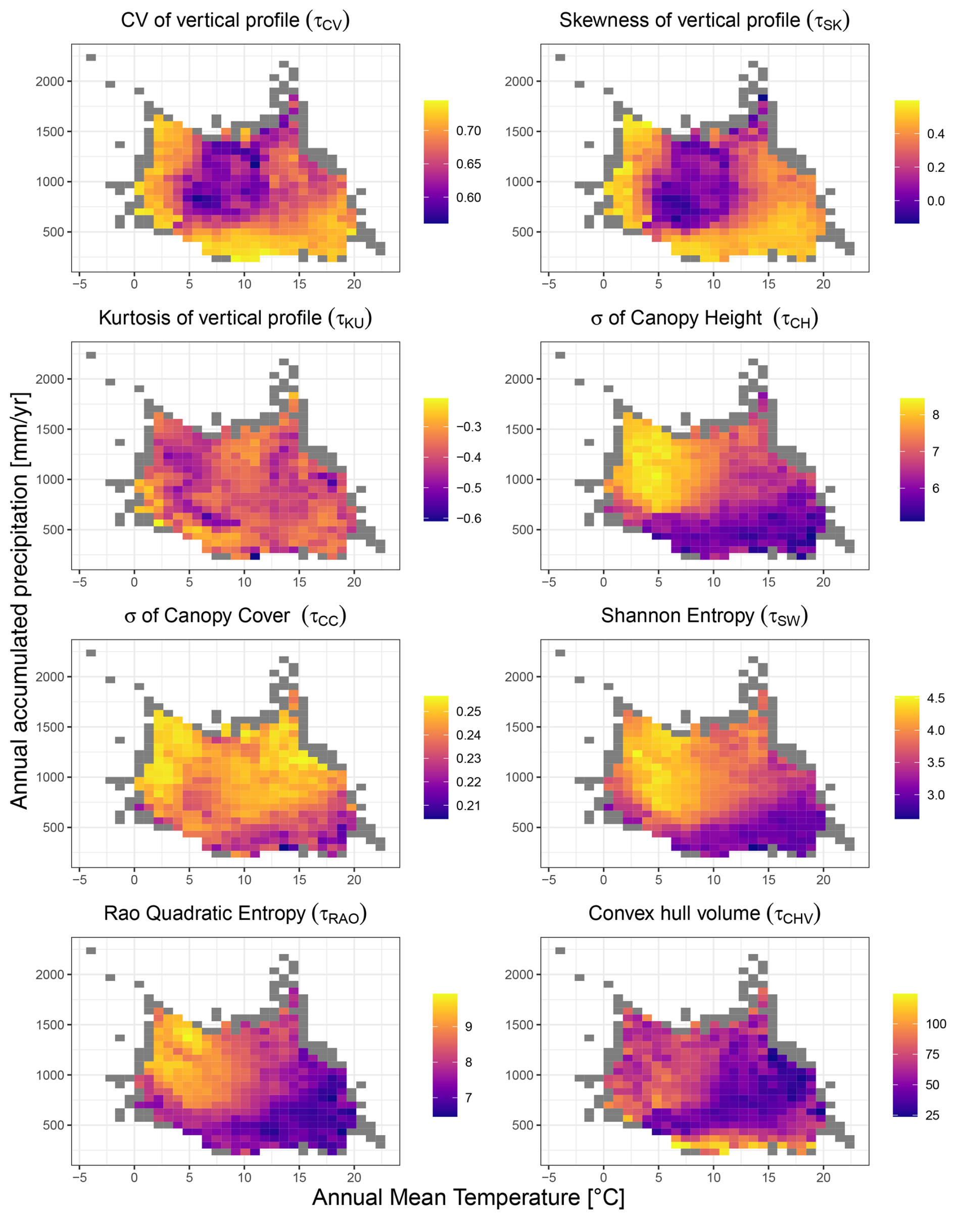
Figure 3 Structural diversity variables mapped against mean climate (temperature and precipitation). The results refer to the dataset at 10 km resolution. Coloured bins depict variation in structural diversity, calculated as the average of the structural diversity values falling within each bin. Grey bins indicate those containing fewer than 5 observations, for which the average was not calculated.

An examination of the variability in the 10 km resolution metrics in climate space revealed distinct patterns along temperature and precipitation gradients (Fig. 3). Patterns of variability in metrics describing vertical heterogeneity showed significant differences when comparing the coefficient of variation (τ_CV) and skewness (τ_SK) against kurtosis (τ_KU). The coefficient of variation and skewness primarily exhibited high values at the extremes of the climatic gradient. This is observed in warm and arid climates where total annual precipitation is below ∼ 500 mm and Annual Mean Temperature is above ∼ 10 °C, as well as in colder climates where Annual Mean Temperature is below ∼ 5 °C. Patterns of variability in the kurtosis were more nuanced, consistently showing negative values across the European domain, which suggests a tendency for a platykurtic distribution in the vertical profile of canopies under diverse environmental conditions. The most pronounced negative kurtosis values were observed for the northern part of the temperate climate zone (Fig. 3). By contrast, more heterogeneous patterns occurred in other areas such as those with a Mediterranean climate, showing high variability (Fig. 3). Diversity metrics describing structural heterogeneity in horizontal space, as well as combined metrics, (τ_CH ,τ_CC, τ_SW, τ_RAO, τ_CVH) also showed considerable variability along precipitation and temperature gradients. With the exception of the convex hull (τ_CVH), all metrics displayed low diversity values in hot and dry climates.

Specifically, a combination of precipitation levels below ∼ 500 mm and annual mean temperatures above ∼ 10 °C (Fig. 3) was associated with the lowest levels of diversity. By contrast, the highest levels of diversity generally occurred in areas with higher precipitation levels (> 500 mm). Patterns of variability in the metrics in climate space for 5 and 1 km resolution (see Figs. S5 and S6 in the Supplement) dataset were broadly concordant with the 10 km dataset, indicating that the results are insensitive to the grain size at which they were calculated.

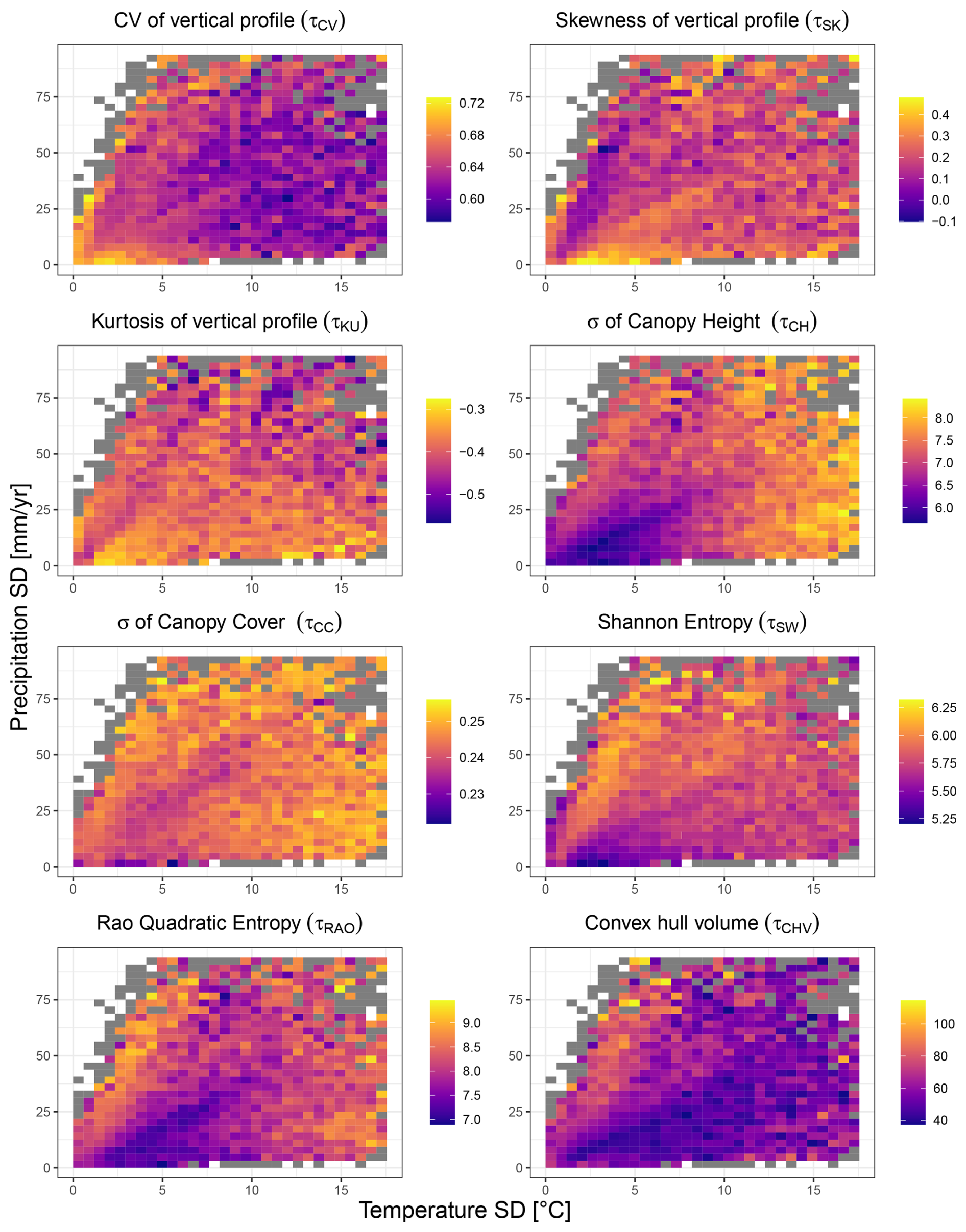
Figure 4 Structural diversity variables mapped against climate variability (temperature and precipitation SD in space). The results refer to the dataset at 10 km resolution. Coloured bins depict variation in structural diversity, calculated as the average of the structural diversity values falling within each bin. Grey bins indicate those containing fewer than 5 observations, for which the average was not calculated.

An examination of the 10 km resolution structural diversity metrics along gradients of temperature and precipitation variability (Fig. 4) revealed distinct but less pronounced patterns compared to those observed in mean climate space (Fig. 3).

Several metrics showed contrasting responses to climate variability. The coefficient of variation of the vertical profile (τ_CV) exhibited an inverse pattern, with highest values occurring at low climate variability (low SD in both temperature and precipitation), suggesting that stable climates may promote more heterogeneous vertical canopy structures. In contrast, the standard deviation of canopy height (τ_CH) showed the most striking pattern, exhibiting high values when temperature variability exceeded 10 °C and precipitation variability fell below 25 mm. Kurtosis (τ_KU) showed relatively modest variation across climate variability space, with a weak tendency toward more negative values (more platykurtic distributions) at higher precipitation variability. The standard deviation of canopy cover (τ_CC) showed a clear vertical gradient, with values increasing primarily as a function of precipitation variability, relatively independent of temperature variability. Similarly, Shannon entropy (τ_SW) was highest at high levels of precipitation variability combined with low to moderate temperature variability. In contrast, Rao's quadratic entropy (τ_RAO) exhibited a bimodal pattern, reaching its highest values both at very low precipitation and low temperature and, to a lesser extent, at high precipitation variability. The convex hull volume (τ_CHV) showed the most uniform distribution across climate variability space, with generally low values and limited systematic variation. Overall, metrics displayed considerably more scatter along gradients of climatic variability than in mean climate space, suggesting that climate variability plays a more complex role in shaping forest structural diversity than mean climate conditions.

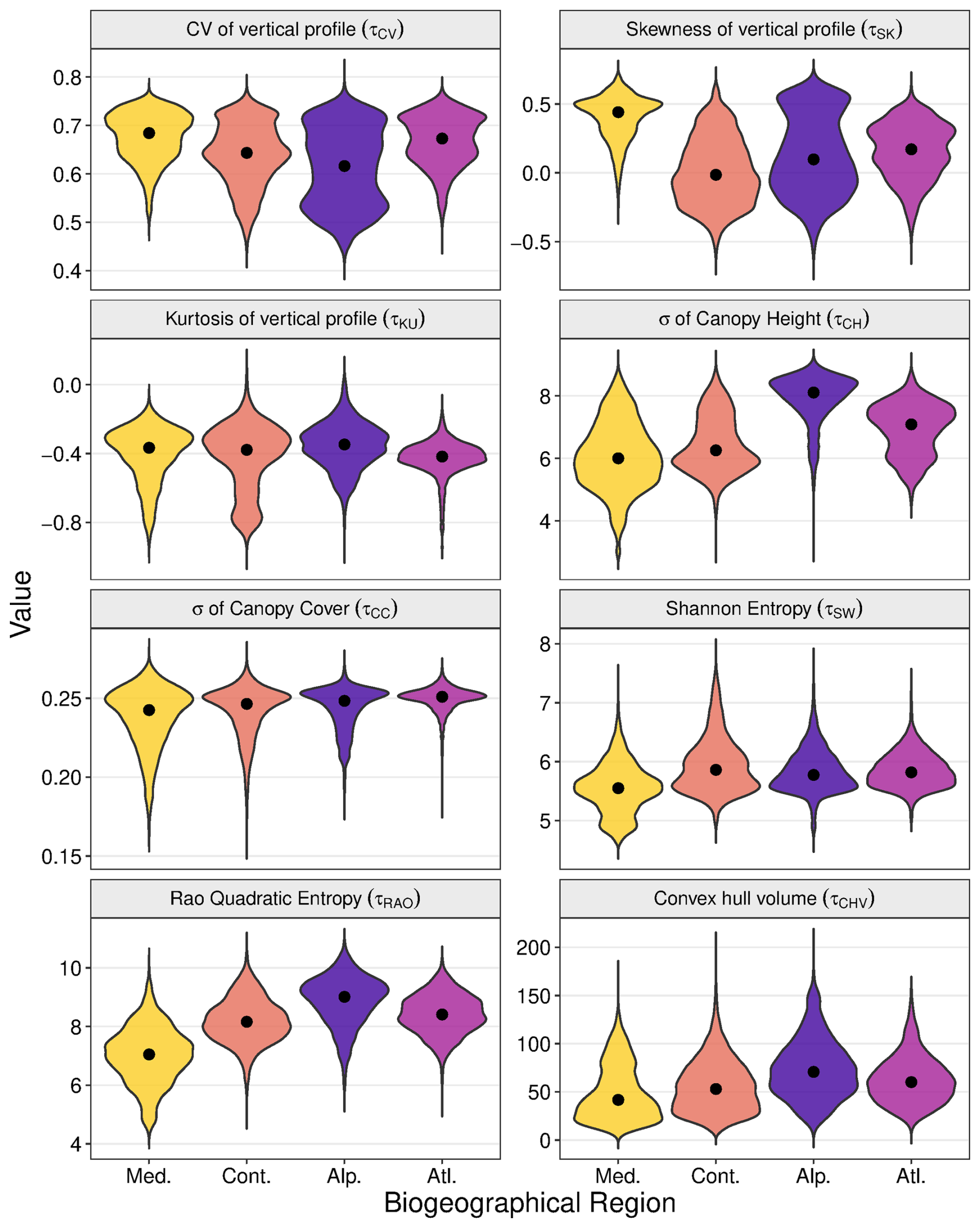
Figure 5 Patterns of variability in forest structural diversity metrics across European biogeographic regions. Violin plots depict the probability density distribution of eight metrics at 10 km resolution. Width represents the kernel density estimate, with black points indicating median values. Colors denote the five biogeographic regions analysed. Med. = Mediterranean region, Cont. = Continental region, Alp. = Alpine region, Atl. = Atlantic region.

An examination of structural diversity patterns by biogeographic region largely reinforced the patterns revealed in the climate space plots (Fig. 5, see Figs. S7 and S8 in the Supplement for the 5 and 1 km datasets), while revealing additional topographic effects. Combined horizontal-vertical diversity metrics (Shannon, Rao) were lowest in the Mediterranean region, consistent with the low diversity observed in hot, arid climates, and highest in Continental, Atlantic, and Alpine regions. Conversely, vertical canopy heterogeneity (Skewness τ_SK) was highest in the Mediterranean region, reinforcing the pattern of elevated skewness at climatic extremes. Canopy height variability (τ_CH) was markedly elevated in the Alpine region (M_ed=8.11) compared to Mediterranean (M_ed=6.00), Continental (M_ed=6.26), and Atlantic (M_ed=7.09), regions likely reflecting greater topographic heterogeneity. CV of vertical profile remained consistent across all regions (∼ 0.65–0.70), while (τ_KU) and σ of canopy cover τ_CC, showed minimal biogeographic variation.

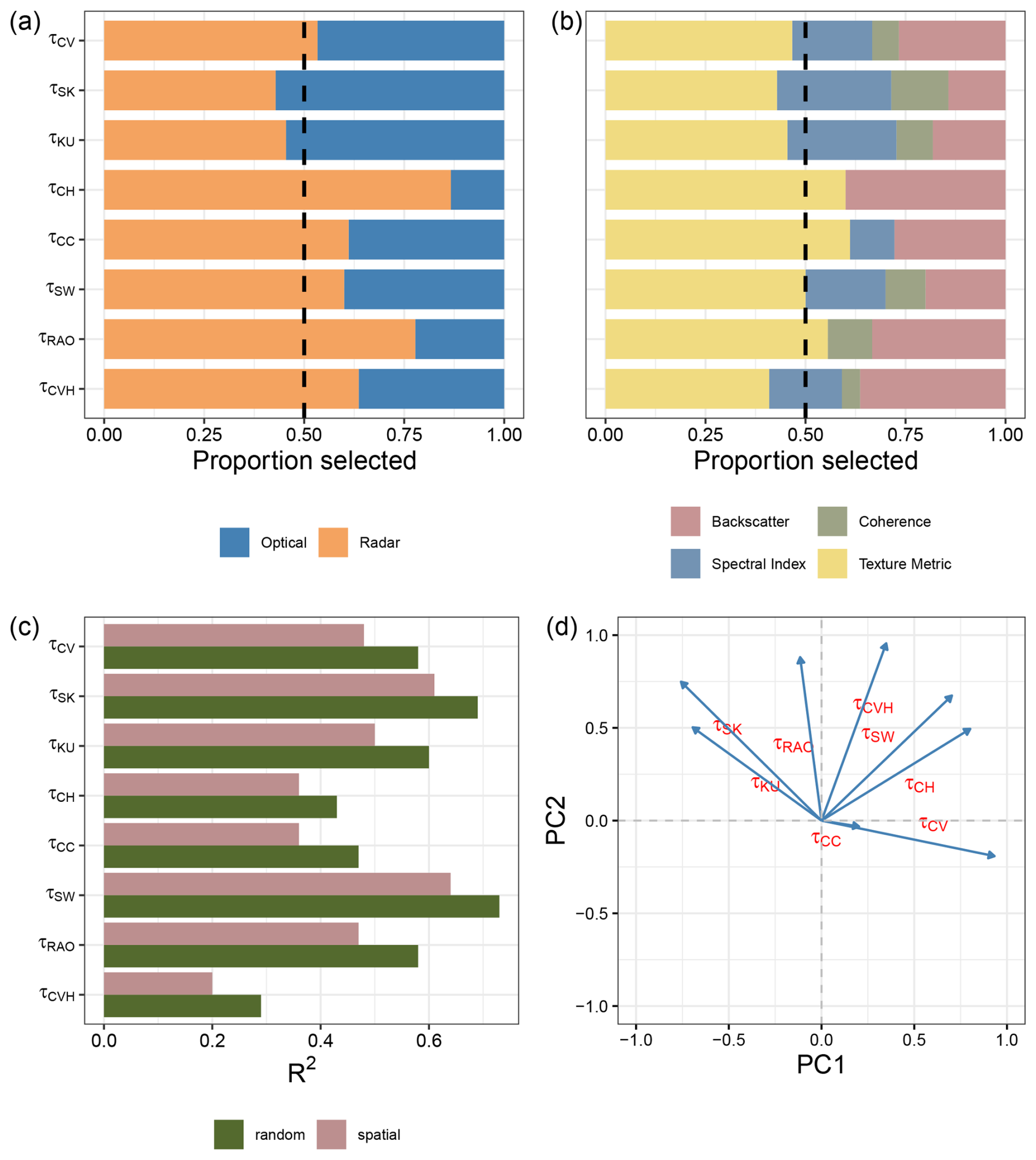
Figure 6 Results of the random forest modelling exercise at 10 km resolution. Panels display the variable selection frequencies (a, b) and model performance, as indicated by the R² values derived from two types of validation methods (c). Panel (d) shows the results of the Principal Component Analysis (PCA) conducted on the estimated structural diversity metrics at this resolution.

A Principal Component Analysis (PCA) biplot (Fig. 6d) was used to explore the degree of intercorrelation among the eight structural diversity metrics. The PCA shows that the metrics are distributed across the principal component space with generally wide angular separation among vectors, indicating low to modest correlations. These patterns are consistent across spatial resolutions (Figs. S9, S11d and S12d in the Supplement).

3.2 Variable importance and model performance

The final models, derived from the stepwise backward elimination procedure, retained between 7 and 23 predictors, representing the extremes observed across various resolutions of input data and output variable types. The number of selected predictors generally increased with the resolution of the input data (Fig. S10 in the Supplement). Models trained for standard deviation of canopy cover (τ_CC) and convex hull (τ_CVH) retained the highest number of predictors. In contrast, models for skewness (τ_SK) and Rao quadratic entropy (τ_RAO) retained the lowest number of predictors (Fig. S10 in the Supplement).

An examination of the type of predictors selected in the final models highlighted the importance of radar-related predictors, over optical ones as shown in Fig. 6a (see Figs. S11a and S12a in the Supplement for the 5 and 1 km datasets). The average proportion of radar-related variables selected across all diversity metrics and resolutions was 0.64, although there was considerable variability. In general, as the resolution of the input dataset increased, the proportion of radar-related variables selected through the feature elimination procedure also increased (Fig. 6a; for the 5 and 1 km datasets see Figs. S11a and S12a in the Supplement). The diversity variables for which the highest number of radar-related predictors were selected was the convex hull (τ_CVH). On the other hand, the one for which the highest number of optical-related predictors were selected, was canopy cover (τ_CC).

Among the predictors retained in the final models, texture-related types were the most commonly selected, followed by backscatter, spectral indices, and coherence (Fig. 6b; for the 5 and 1 km datasets see Figs. S11b and S12b in the Supplement). Notably, texture metrics constituted, on average, the largest proportion of selected variables at a 10 km resolution (Fig. 6b). Conversely, the proportion of backscatter-related variables and spectral indices increased in models using the finer resolution input data (Figs. S11b and S12b in the Supplement).

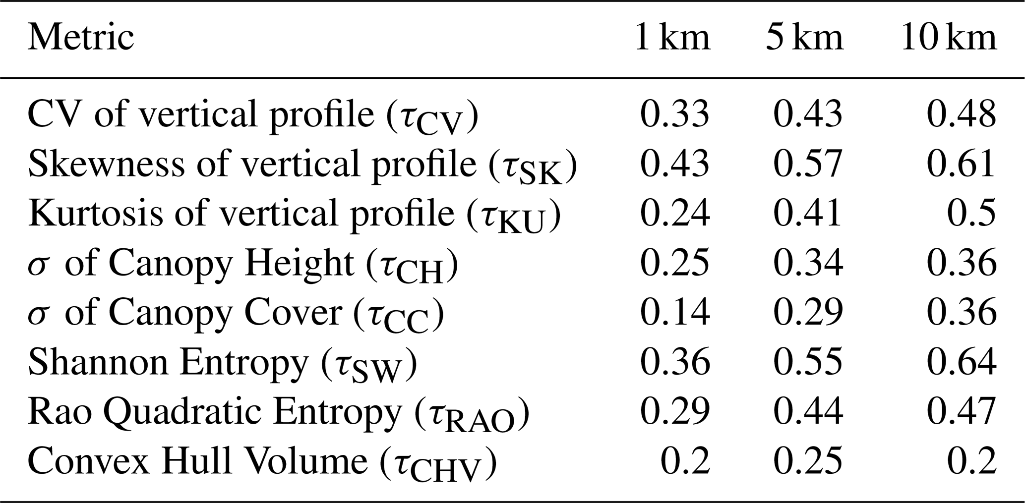
Model validation revealed that random cross-validation consistently outperformed spatial cross-validation across all resolutions. At 10 km resolution, the model for the Shannon the model for Shannon index τ_SW achieved the highest scores, with 0.73 in random validation and 0.64 in spatial validation (Fig. 6c and Tables B1 and B2). Conversely, the model with convex hull (τ_CVH) as a variable showed the lowest performance, scoring 0.29 in random cross-validation and 0.20 in spatial cross-validation. This difference likely reflects the contrasting statistical properties of the metrics: Shannon entropy integrates information across the full distribution of GEDI observations within a spatial unit and is therefore more robust to sampling variability, whereas convex hull–based metrics are more sensitive to outliers and local sampling density.The best-performing models at 5 and 1 km differed from those at 10 km, with skewness models (τ_SK) yielding the best results at both 5 and 1 km, while canopy cover variability (τ_CC) was the lowest-performing at 1 km and convex hull (τ_CVH) at 5 km (Tables B1 and B2; Figs. S11c and S12c in the Supplement).

Models estimating metrics describing horizontal variability, particularly the standard deviation of canopy cover (τ_CC) and convex hull volume (τ_CVH), showed lower predictive performance, especially at finer spatial resolutions (R² < 0.30 at 1 km). These metrics rely more directly on variability among individual GEDI observations within a spatial unit, which is less consistently preserved when locally derived optical and SAR predictors are spatially aggregated to the grid-cell level. In contrast, models estimating metrics describing vertical heterogeneity and combined structural diversity (e.g. τ_SK, τ_CV, τ_SW), particularly at 10 km resolution, exhibited higher validation scores and greater stability across validation schemes.

An examination of the standard deviation of model outputs revealed generally increasing trend of prediction uncertainty across resolutions (Figs. S13, S14 and S15 in the Supplement), except in Rao (τ_RAO) and convex hull (τ_CVH). Overall, uncertainty was generally low across the spatial domain of interest, reflecting limited variability within the ensemble. Notable exceptions occur in the Mediterranean region for the convex hull, kurtosis, and standard deviation of canopy height metrics. Further variability is observed in Eastern Europe, particularly for the convex hull, skewness, kurtosis, Shannon index, and standard deviation of canopy height.

4 Discussion

4.1 Model-based predictions of structural diversity

Our dataset provides eight metrics describing the structural heterogeneity of European forests. To our knowledge, this is the first attempt to comprehensively map forest structural diversity at a quasi-continental scale (because GEDI is unable to observe anything above 50° N). Datasets such as the one presented here contribute to an emerging landscape of data products based on spaceborne LiDAR data, ranging from regional to global scales (e.g. Lang et al., 2023; Shendryk, 2022; Sothe et al., 2022). However, while most efforts have primarily focused on mapping top canopy height, we aimed to create a set of complementary metrics describing the diversity of canopy structure, an ecologically important yet neglected aspect in research.

Some of the ecological indices employed in this study are routinely applied to optical data to quantify landscape-level heterogeneity using multispectral data (Tuanmu and Jetz, 2015). For instance, the Rao and Shannon diversity indices, which can be calculated from spectral indices, have been widely used to quantify the heterogeneity of vegetation and are often proposed as indicators of ecosystem heterogeneity (Rocchini et al., 2021). These heterogeneity indicators have proved to be useful in a variety of contexts, including biodiversity modelling and quantifying the vulnerability of forest ecosystems to disturbances (Forzieri et al., 2021; Taddeo et al., 2021). However, indices based solely on optical data fail to capture crucial aspects of structural heterogeneity, which are related to the three-dimensional arrangement of vegetative elements in the canopy (Fassnacht et al., 2022). Our study addresses a critical gap by introducing the first consistent dataset that maps structural diversity across the forested domain in Europe. This development will contribute to a more detailed and robust regional analysis on ecosystem dynamics, which critically depend on vegetation structure (Migliavacca et al., 2021) and structural diversity (LaRue et al., 2023), and other facets of biodiversity, which requires information on the vertical profile of plants (Fassnacht et al., 2022).

Our findings revealed that model performance differed according to the spatial resolutions and diversity metrics, with several models achieving R² values indicative of moderate to strong predictive accuracy, particularly at coarser spatial resolutions (Appendix B, Tables B1 and B2). This variation highlights the critical role of resolution in model performance, indicating that, depending on the application of interest, coarser resolutions may optimize the utility of the models. As expected, spatial cross-validation consistently yielded lower R² values than random train-validation random validation across most metrics and resolutions. This outcome reflects the challenges inherent on machine learning methods (Meyer and Pebesma, 2021) of predicting outcomes in areas geographically distinct from the training data. Neverthless, the decrease was generally modest, affirming the broad applicability of our models beyond the training domain.

The recursive feature elimination procedure highlighted the importance of textural variables (Fig. S10 in the Supplement) across diversity metrics and spatial resolutions. Entropy, derived from ALOS-PALSAR-2 data, stood out as the most influential variable, corroborating research that demonstrates textural metrics' effectiveness in capturing spatial heterogeneity in structural diversity (Bae et al., 2019). Additionally, the significant role of coherence, which aligns with evidence of its predictive power for forest structural features (Bruggisser et al., 2021; Cartus et al., 2022), suggests its potential in reflecting changes in forest structural density and composition. Collectively, our findings underscore the benefits of integrating various sensor data to enhance the prediction of structural diversity, as evidenced by the diverse contributions of optical and radar-based predictors.

4.2 Potential applications

We envisage that our structural diversity dataset will significantly advance future research and practical applications across several disciplines. We identify three key areas where the dataset could be utilised.

Firstly, the dataset could aid in the development of different biodiversity indicators. Ecosystem structure has been identified as an Essential Biodiversity Variable (EBV) (Valbuena et al., 2020), and a wide range of studies have shown a strong correlation between LiDAR-based metrics and ground-based biodiversity measurements (Marselis et al., 2020). The metrics developed here could be used to identify areas with unique structural features that harbour high levels of biodiversity. Furthermore, integrating them with data from other sensors, such as Sentinel 1 and Sentinel 2, offers a promising avenue for generating accurate spatial explicit estimates of different indicators, thus paving the way for the development of frameworks for monitoring long-term biodiversity changes.

Secondly, the dataset offers a valuable resource for quantifying the observed impacts of global change drivers on the functioning of European forest ecosystems. The increasing recognition of the role of structural diversity in driving ecosystem processes (Ali et al., 2016; Aponte et al., 2020; Listopad et al., 2015) underscores the importance of our metrics. Consequently, our dataset provides a crucial tool for enabling comprehensive, data-driven assessments of the impact of climate and land cover changes on the functioning of forest ecosystems across large scales, addressing the previous limitations posed by the unavailability of structural diversity data over extensive spatial scales.

Thirdly, the dataset could be used for improving Earth system models. Historically, plant canopy structure has not been adequately represented in these models (Atkins et al., 2018; Schneider et al., 2020). This lack of detailed representation can lead to significant errors in predicting energy balance, carbon cycling, and ecosystem responses to environmental changes (Duveiller et al., 2023). Integrating structural diversity into these models has the potential to enhance the accuracy of simulations by incorporating more realistic representations of light interception, photosynthetic rates, and energy fluxes. In particular, these applications are directly relevant to contemporary Earth system modelling frameworks such as CMIP6 and forthcoming CMIP7 simulations, which underpin IPCC climate assessments and projections.

5 Data availability

The structural diversity metrics generated in this study can be accessed at Figshare: https://doi.org/10.6084/m9.figshare.26058868.v1 (Girardello et al., 2024). All maps are available at three spatial resolutions (1, 5, and 10 km) in the EPSG:3035 (LAEA) spatial reference system. All eight at all three spatial resolutions are provided; users are encouraged to consult the validation results (Tables B1 and B2) to assess the suitability of individual metrics for specific applications.

6 Code availability

The code developed for data preparation and figure reproduction is publicly available in a Figshare repository (Figshare; https://doi.org/10.6084/m9.figshare.26058868.v1, Girardello et al., 2024).

7 Conclusions

We generated a spatially-explicit dataset on eight forest structural diversity metrics at multiple resolutions (10, 5, 1 km) encompassing temperate, Mediterranean, and continental regions of Europe. Models developed to create the dataset were robust. The dataset generated in our study represents a novel contribution to the Essential Biodiversity Variables (EBV) framework, and the metrics can be used in various applications, ranging from the study of biodiversity to ecosystem functioning. We conclude that combining GEDI data with those from other satellite sensors paves the way for developing a consistent and scalable framework to monitor structural diversity across Europe.

Appendix A: Supplementary Methods

A1 Statistical indicators

The statistical indicators used in this study are detailed below. The mean μ, standard deviation σ, skewness γ, excess kurtosis κ, coefficient of variation cv of a variable $X=\left\{x_{\mathrm{1}},\mathrm{\dots },x_N\right\}$ are defined as:

$$\begin{array}{}\text{(A1)}& \begin{array}{rl}& \mathit{\mu }\left(X\right)={\displaystyle \frac{\mathrm{1}}{N}}{\sum }_{i=\mathrm{1}}^N{x}_i\\ & \mathit{\sigma }\left(X\right)=\left\{{\displaystyle \frac{\mathrm{1}}{N}}{\sum }_{i=\mathrm{1}}^N{\left[x_i-\mathit{\mu }\left(X\right)\right]}^{\mathrm{2}}\right\}\\ & \mathit{\gamma }\left(X\right)={\displaystyle \frac{{\sum }_{i=\mathrm{1}}^N{\left[x_i-\mathit{\mu }\left(X\right)\right]}^{\mathrm{3}}}{{\left[\mathit{\sigma }\left(X\right)\right]}^{\mathrm{3}}}}\\ & \mathit{\kappa }\left(X\right)={\displaystyle \frac{{\sum }_{i=\mathrm{1}}^N{\left[x_i-\mathit{\mu }\left(X\right)\right]}^{\mathrm{4}}}{{\left[\mathit{\sigma }\left(X\right)\right]}^{\mathrm{4}}}}\\ & \mathrm{cv}\left(X\right)={\displaystyle \frac{\mathit{\sigma }\left(X\right)}{\mathit{\mu }\left(X\right)}}\end{array}\end{array}$$

A2 Binning in cartesian 4d space

p_επoω indicates the fraction of the GEDI shots falling in the bin identified by the indices $\left(\mathit{\epsilon },\mathit{\pi },o,\mathit{\omega }\right)$ in the 4D cartesian space defined on the basis $\left(e^{\mathit{\epsilon }},e^{\mathit{\pi }},e^o,e^{\mathit{\omega }}\right)$, see Fig. S2, with

$$\begin{array}{}\text{(A2)}& {\sum }_{\mathit{\epsilon }\mathit{\pi }o\mathit{\omega }}{p}_{\mathit{\epsilon }\mathit{\pi }o\mathit{\omega }}=\mathrm{1}\end{array}$$

where ∑_επoω stands for ${\sum }_{\mathit{\epsilon }=\mathrm{1}}^{N_{\mathrm{bins}}^{e^{\mathit{\epsilon }}}}{\sum }_{\mathit{\pi }=\mathrm{1}}^{N_{\mathrm{bins}}^{e^{\mathit{\pi }}}}{\sum }_{o=\mathrm{1}}^{N_{\mathrm{bins}}^{e^o}}{\sum }_{\mathit{\omega }=\mathrm{1}}^{N_{\mathrm{bins}}^{e^{\mathit{\omega }}}}$, with $N_{\mathrm{bins}}^{e^{\mathit{\epsilon }}}$ number of bins in the e^ε dimension, and $D_{\mathit{\epsilon }\mathit{\pi }o\mathit{\omega }}^{{\mathit{\epsilon }}^{\prime }{\mathit{\pi }}^{\prime }{o}^{\prime }{\mathit{\omega }}^{\prime }}$ indicates the cartesian distance between $\left(\mathit{\epsilon },\mathit{\pi },o,\mathit{\omega }\right)$ and $\left({\mathit{\epsilon }}^{\prime },{\mathit{\pi }}^{\prime },o^{\prime },{\mathit{\omega }}^{\prime }\right)$ bin.

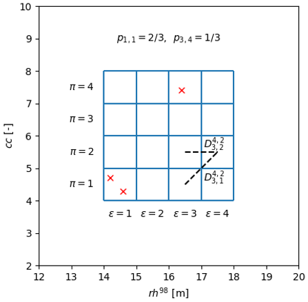
Figure A1 Example of p_επ and $D_{\mathit{\epsilon }\mathit{\pi }}^{{\mathit{\epsilon }}^{\prime }{\mathit{\pi }}^{\prime }}$ estimation in the 2D cartesian space defined on the basis (rh⁹⁸,cc). The GEDI shots are reported with the red X, GEDI cc values have been amplified by 10.

A3 Predictor calculation

Starting with appropriate bands/indices (step 2 of the workflow in the main text), the four scalars ${\mathit{\varphi }}_{\mathit{\alpha },i}^{\mathit{\beta }}$, where $\mathit{\beta }\in \left\{\mathrm{SM},\mathrm{ASM},\mathrm{ENT},\mathrm{DISS}\right\}$, are calculated from the cluster of 7 × 7 pixels ${\mathit{\varphi }}_{\mathit{\alpha },i}(p,q)$ overlapping the footprint of the GEDI shot i, where p and q represent the pixel indices within the window. In details, we calculated:

1. the spatial mean (SM)

   $$\begin{array}{}\text{(A3)}& {\mathit{\varphi }}_{\mathit{\alpha },i}^{\mathrm{SM}}=\mathit{\mu }\left({\mathit{\varphi }}_{\mathit{\alpha },i}\left(p,q\right)\right)\end{array}$$

   which is performed to compensate for potential footprint geolocation inaccuracies, and reduce the presence of noise, and three texture metrics. Texture metrics provide spatial content information (Nichol and Sarker 2011), and are highly effective in capturing the pixels heterogeneity. Defining ${\stackrel{\mathrm{‾}}{\mathit{\varphi }}}_{\mathit{\alpha },i}(p,q)$ as the grey-levels matrix, which is calculated from ${\mathit{\varphi }}_{\mathit{\alpha },i}(p,q)$ by normalizing the values¹ within the range of [0, 1] based on the 1st and 99th percentiles, $C_{\mathit{\alpha },i}(m,n)$ as the corresponding grey-levels co-occurrence matrix (GLCM), with dimension 256 × 256 (Haralick et al. 1973):

   $$\begin{array}{rl}& C_{\mathit{\alpha },i}(m,n)={\sum }_{p=\mathrm{1}}^{\mathrm{7}}{\sum }_{q=\mathrm{1}}^{\mathrm{6}}\mathrm{1},\\ & \mathrm{if}{\stackrel{\mathrm{‾}}{\mathit{\varphi }}}_{\mathit{\alpha },i}\left(p,q\right)=m\mathrm{and}{\stackrel{\mathrm{‾}}{\mathit{\varphi }}}_{\mathit{\alpha },i}\left(p,q+\mathrm{1}\right)=q;\\ & \mathrm{0},\mathrm{otherwise}\end{array}$$

   and $p_{\mathit{\alpha },i}(m,n)$ as the probability that grey-level m occurs close to the grey-level n:

   $$\begin{array}{}\text{(A4)}& p_{\mathit{\alpha },i}(m,n)={\displaystyle \frac{C_{\mathit{\alpha },i}(m,n)}{{\sum }_{p=\mathrm{0}}^{\mathrm{255}}{\sum }_{q=\mathrm{0}}^{\mathrm{255}}{C}_{\mathit{\alpha },i}\left(p,q\right)}}\end{array}$$

   we calculated:

2. the angular second moment (ASM)

   $$\begin{array}{}\text{(A5)}& {\mathit{\varphi }}_{\mathit{\alpha },i}^{\mathrm{ASM}}=-{\sum }_{m=\mathrm{0}}^{\mathrm{255}}{\sum }_{n=\mathrm{0}}^{\mathrm{255}}{\left[p_{\mathit{\alpha },i}(m,n)\right]}^{\mathrm{2}}\end{array}$$

   ASM is a measure of the homogeneity or uniformity of pixel values within a neighbourhood. It reflects the degree to which pixel values deviate from the mean, providing insights into the texture's smoothness or roughness;

3. the entropy

   $$\begin{array}{}\text{(A6)}& \begin{array}{rl}& {\mathit{\varphi }}_{\mathit{\alpha },i}^{\mathrm{ENT}}=\\ & -{\sum }_{m=\mathrm{0}}^{\mathrm{255}}{\sum }_{n=\mathrm{0}}^{\mathrm{255}}{p}_{\mathit{\alpha },i}(m,n)\log p_{\mathit{\alpha },i}(m,n)\end{array}\end{array}$$

   Entropy is a measure of the randomness or disorder in the distribution of grey levels. It quantifies image non-uniformity, with higher entropy values indicating a more random distribution of pixel values within a neighbourhood;

4. the dissimilarity index

   $$\begin{array}{}\text{(A7)}& \begin{array}{rl}& {\mathit{\varphi }}_{\mathit{\alpha },i}^{\mathrm{DISS}}=\\ & {\sum }_{m=\mathrm{0}}^{\mathrm{255}}{\sum }_{n=\mathrm{0}}^{\mathrm{255}}{p}_{\mathit{\alpha },i}(m,n)\left|m-n\right|{\mathrm{ogp}}_{\mathit{\alpha },i}(m,n)\end{array}\end{array}$$

   Dissimilarity measures the complexity and the nature of grey-level transitions among neighbouring pixels (Conners et al. 1984). It quantifies image contrast, with higher dissimilarity values reflecting pronounced differences among neighbouring pixel values.

Appendix B: Model validation results

Table B1 Results of the random validation procedure conducted for the forest structural metrics at three spatial resolutions: 1 × 1, 5 × 5, and 10 × 10 km. The validation outcomes are presented in terms of the coefficient of determination (R²), which quantifies the proportion of the variance in the dependent variable that is predictable from the independent variables.

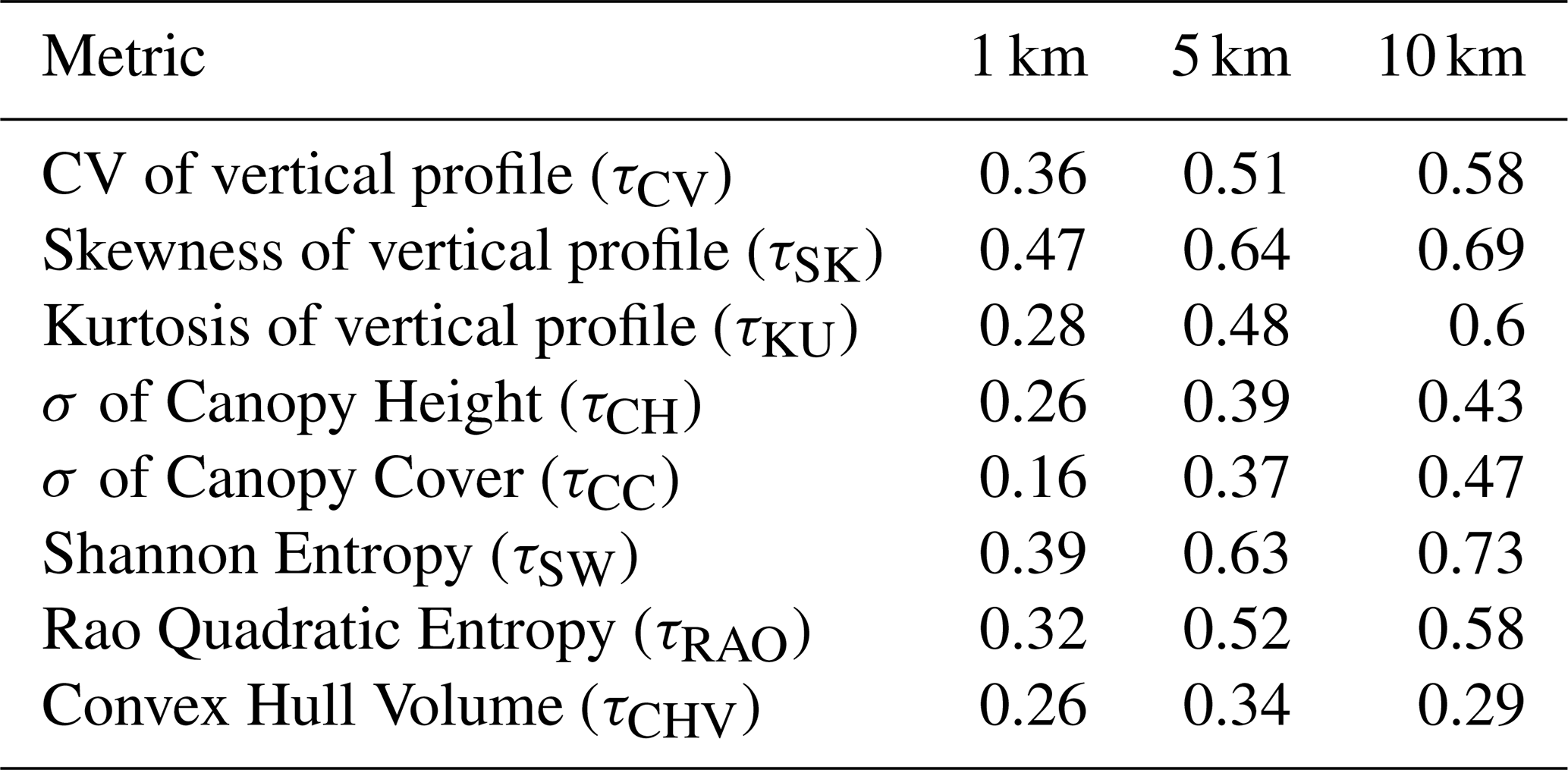
Table B2 Results of the spatial cross-validation procedures conducted for the forest structural metrics at three spatial resolutions: 1 × 1, 5 × 5, and 10 × 10 km. The validation outcomes are presented in terms of the coefficient of determination (R²).