Spatially distributed measurements of aerosols and stable isotopes in water vapour and precipitation in coastal Northern Norway during the ISLAS2021 campaign

Precipitation from mixed-phase clouds at high-latitudes is difficult to represent correctly in numerical weather prediction models. Paired water vapour and precipitation isotope measurements provide a constraint on the integrated effect of evaporation and condensation processes, but have rarely been collected in a way that allows to use these for model validation and improvement. Here we present a collection of spatially distributed measurements of water isotopes in the different phases at high time resolution during the ISLAS2021 field campaign over the period 15 to 30 March 2021. The main observational site of this campaign was Andenes, Norway (69.3144° N, 16.1194° E). Isotopic measurements were conducted simultaneously at sea level and a mountain observatory, as well as additional coastal sites at distances of 120 km (Tromsø, Norway) and 1100 km (Bergen, Norway), enabling the assessment of spatial representativeness of vapour isotope measurements. Precipitation samples for water isotope analysis were collected on site at sub-event time resolution, and along a transect across the Vesterålen archipelago. These measurements were complemented by a suite of aerosol measurements, including ice-nucleating particles, and additional in situ and remote sensing observations of meteorological variables. During the two weeks of the ISLAS2021 field campaign, frequent alternations between mid-latitude and arctic weather systems were encountered, providing a range of different cases for more detailed process studies. The dataset is available at https://doi.org/10.1594/PANGAEA.984616 (Sodemann et al., 2025), and can serve as a test bed for assessing the spatial representativeness and sampling strategies for water isotope measurements on meteorological time scales. Furthermore, we anticipate our data to be useful in various aspects related to cloud microphysics, for example the quantification of riming processes in convective clouds, the role of ice nucleating particles in marine cold-air outbreaks, and on the condensation efficiency of mid-latitude storms.

1 Introduction

Numerical weather prediction and climate models tend to misrepresent the partitioning of liquid and ice cloud water, cloud cover fraction and the transition between different cloud types (Sandu and Stevens, 2011), in particular at high latitudes (Field et al., 2017). This misrepresentation can lead to biases in model predictions of the surface energy balance, air temperature, and precipitation amount and intensity (Shupe and Intrieri, 2004; Stevens et al., 2018). Moreover, some model deficiencies may be difficult to unveil due to compensating errors. For example, in a case of arctic stratocumulus clouds simulated by the numerical weather prediction model AROME-Arctic (Müller et al., 2017b, a), compensation between physical and dynamical tendencies has been identified (Kähnert et al., 2021), affecting specific humidity in the atmospheric boundary layer and ensuing formation of cloud liquid water and cloud ice.

Furthermore, there is still a limited understanding of aerosol-cloud interactions, and processes controlling the moisture budget and the phase distribution in arctic clouds (Morrison et al., 2012). A subset of cloud forming aerosols, termed cloud condensation nuclei and ice-nucleating particles (INPs), control the number of cloud droplets and primary ice crystals in clouds, respectively. The concentration and size of cloud droplets and ice crystals, and their respective ratios, influence cloud radiative properties, precipitation formation and cloud lifetime (e.g. Cantrell and Heymsfield, 2005). However, as the concentration of INPs in the Arctic is still poorly constrained, representing the correct concentration of ice crystals in arctic clouds in Earth System Models (ESMs) is challenging (Murray et al., 2021). Thus, accurately representing the impact of these clouds on the present-day and future climate in ESMs is uncertain (Tan et al., 2016; Bjordal et al., 2020; Zelinka et al., 2020; Forster et al., 2021).

Observational campaigns are key in providing the necessary data basis to derive process understanding, and to enable numerical model evaluation and development. Data obtained during the COMBLE field campaign at the coast of Northern Norway (Geerts et al., 2022), as well as measurements obtained at Ny-Ålesund, Svalbard within the ACTRIS network (Ebell et al., 2025), demonstrate the value of combined in-situ and remote-sensing instrumentation to quantify cloud properties, precipitation, and microphysical processes of high-latitude mixed-phase clouds. To address compensating errors in model parameterisations, additional observational quantities are needed to constraint models to the real-world atmosphere. The stable isotope composition of precipitation has long been used on climate to weather time scales (Jouzel, 2013; Galewsky et al., 2016). The potential of combined measurements of water vapour and precipitation isotopes to reveal information about phase changes on microphysical time scales has, however, so far only rarely been exploited (Lowenthal et al., 2016; Graf et al., 2019; Weng et al., 2021).

Stable water isotopologues (H${}_{\mathrm{2}}^{\mathrm{16}}$O, H²H¹⁶O, and H${}_{\mathrm{2}}^{\mathrm{18}}$O), here collectively referred to as stable water isotopes (SWI), are naturally occurring tracer quantities in the water cycle. During phase changes, including evaporation and condensation, heavier isotopes prefer the solid and liquid phase over the vapour phase, a process known as temperature-dependent isotope fractionation (e.g., Galewsky et al., 2016). Thereby, the vapour and precipitation signals co-evolve over the time scale of weather systems, producing regional patterns of isotope depletion (Dütsch et al., 2018), that may reflect the time-integrated effect of condensational processes. As evaporation, mixing, condensation and precipitation processes proceed along the transport pathway of air masses, the isotope signal further evolves in terms of δ²H and δ¹⁸O in water vapour and precipitation, creating an integrated reflection of the atmospheric processing of water vapour. Hereby, the δ symbol represents a deviation of the isotope ratio between rare and abundant isotopes compared to an internationally agreed reference (Vienna Standard Mean Ocean Water, VSMOW) in units of ‰ (IAEA, 2017).

In a strongly undersaturated or supersaturated environment, the differences in the diffusion speed between H²H¹⁶O (HDO), H${}_{\mathrm{2}}^{\mathrm{18}}$O and H${}_{\mathrm{2}}^{\mathrm{16}}$O give rise to non-equilibrium fractionation, quantified in terms of the Deuterium excess:

$$\begin{array}{}\text{(1)}& \mathrm{d}\text{-}\mathrm{excess}=\mathit{\delta }\mathrm{D}-\mathrm{8}\times {\mathit{\delta }}^{\mathrm{18}}\mathrm{O}.\end{array}$$

Pronounced non-equilibrium isotope fractionation occurs for example during marine cold-air outbreaks (mCAOs), when cold and dry air from the Arctic is advected over open ocean (Papritz and Spengler, 2017; Dahlke et al., 2022). In such weather systems, large vertical gradients in relative humidity and high wind speeds create an environment of strong latent heat fluxes. As the HDO molecules diffuse faster than H${}_{\mathrm{2}}^{\mathrm{18}}$O, they become relatively enriched in the evaporation flux compared to less intense evaporation conditions, resulting in a distinct positive d-excess signature from mCAOs (Thurnherr et al., 2021; Duscha et al., 2022; Sodemann et al., 2024). When the mCAO air masses, often characterised by convective cells, reach the coast, the ensuing precipitation may still carry an imprint of the evaporation conditions.

This sensitivity of the isotopic signal to phase changes has been utilised to investigate cloud processes in previous studies (Lowenthal et al., 2016, 2011). In the work of Galewsky (2018), SWI observations were applied to study atmospheric boundary layer and low-cloud processes. Model studies of Dütsch et al. (2019) showed that SWI may be used to constrain microphysical parameters of mixed-phase clouds in supersaturation-enabled models due to the sensitivity of isotopic fractionation to temperature and to the saturation ratio with respect to ice. Other processes that affect the isotopic composition of cloud water and precipitation are the well-known growth of ice crystals at the expense of evaporating cloud droplets at supersaturation with respect to ice (Wegener, 1911; Bergeron, 1928; Findeisen, 1938), collision-coalescence, the simultaneous growth of liquid droplets and ice crystals, and riming in the presence of supercooled liquid (Ciais and Jouzel, 1994; Pruppacher and Klett, 1997; Korolev et al., 2017).

Riming, the freezing of supercooled liquid onto ice crystals, depends on the concentration of cloud forming aerosol or cloud condensation nuclei. As cloud droplet size decreases with a larger number of cloud condensation nuclei, the riming efficiency decreases (Borys et al., 2003; Lowenthal et al., 2016). Furthermore, ice nucleating particles (INPs) in the Arctic show dependence on the distance from and type of source region (e.g., Wex et al., 2019; Carlsen and David, 2022; Creamean et al., 2022). In particular, whether an air mass is advected over open ocean, sea ice, land or snow-covered surface, has a large impact on the concentration of INPs (Bigg and Leck, 2001; Creamean et al., 2018; Hartmann et al., 2020; Tobo et al., 2019; Carlsen and David, 2022). In a similar way as SWI, INPs are preferentially removed by precipitation during transport, and thus in conjunction with stable isotope measurements inform about the fraction of condensed and precipitated water vapour (Stopelli et al., 2015). Thus, combined SWI, aerosol, and INP observations offer new avenues to evaluate microphysical processes (Lowenthal et al., 2011; Moore et al., 2016) and below-cloud exchange (Graf et al., 2019), with the opportunity to improve our understanding of the arctic water cycle, and its representation in numerical models.

While aerosols and gas chemistry are regularly coordinated with cloud microphysical observations (Geerts et al., 2022), INPs have so far, despite their important role for high-latitude clouds (Stopelli et al., 2015), rarely been included in more comprehensive studies. Simultaneous SWI and aerosol measurements in the Arctic with high temporal resolution are limited to very few locations and time periods (e.g., Leroy‐Dos Santos et al., 2020). Even at lower latitudes, the combination of the two methods for cloud studies is still rare (e.g., Lowenthal et al., 2016; Stopelli et al., 2015). Therefore, the ISLAS2021 campaign was focused on obtaining a dataset with both stable water isotope and INP measurements that are tightly integrated with routine meteorological observations to be useful for process studies and evaluation of numerical prediction models.

The sub-arctic latitudes of the Vesterålen archipelago in Northern Norway experience unique variations of pronounced weather systems during northern hemisphere spring. During that season, rapid alterations take place between mCAO conditions, characterised by cold winds and snow showers (Geerts et al., 2022), and warm air intrusions (WAI), associated with warmer temperatures, persistent precipitation, and strong winds, that propagate poleward from the mid-latitudes (Woods and Caballero, 2016). An important characteristic of mCAOs in the Nordic Seas is that their water cycle is confined in space and time by the sea ice edge and the surrounding topography (Fig. 1a). Thus, typical lifetimes of water vapour from evaporation to precipitation can be as short as 1 to 2 d (Papritz and Sodemann, 2018), only a fraction of the global median lifetime of 5–6 d, and substantially shorter than the global mean of 8–10 d (Sodemann, 2020; Gimeno et al., 2021). The spatial and temporal confinement of the moisture source reduces the range of factors potentially contributing to the SWI and aerosol composition.

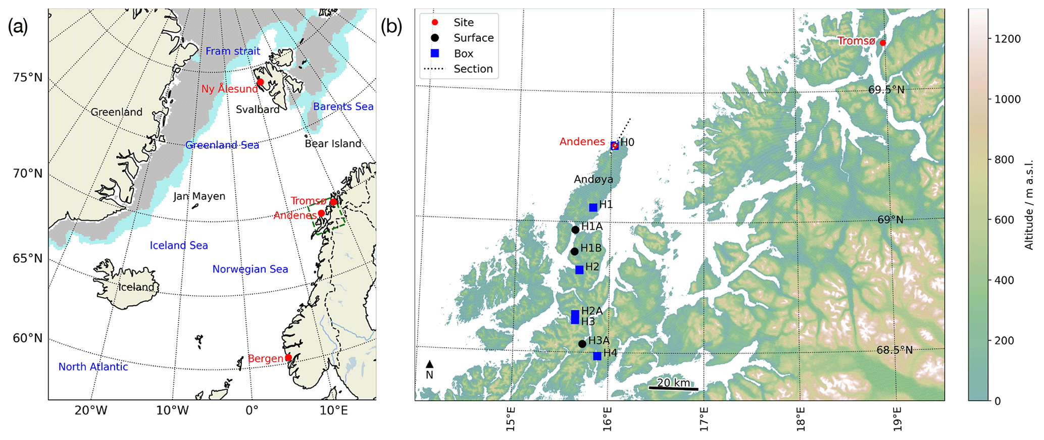
Figure 1 Study region and setup of the ISLAS2021 campaign. (a) Stations with vapour and/or precipitation isotope measurements (red), ocean regions (blue), and key topographic features (black). Shading denotes sea ice concentration above 70 % (grey) and between 30 %–70 % (light blue) from Copernicus Climate Change Service (2020). Green dashed box indicates location of the zoomed map to the right. (b) Regional sampling network in Northern Norway of water vapour isotope measurements sites (red dots), snow sampling boxes (blue squares), surface snow sampling sites (black dots). Dotted line indicates the location of the section shown in Fig. 2a.

Here we describe the setup and sampling activity of the ISLAS2021 measurement campaign conducted during late winter (15 to 30 March 2021) at Andenes, located on Andøya, an island of the Vesterålen archipelago off the coast of Northern Norway (69.2954° N, 16.0337° E) and an additional network of stations. The main scientific aim of the ISLAS2021 campaign was to collect a dataset that would allow for the assessment of water turnover in arctic weather systems with a focus on cloud processes and precipitation. To this end measurements of water vapour and precipitation isotopes, aerosols and INPs were collected across a spatially distributed network focused on coastal Northern Norway. The specific objectives of the campaign were:

1. to continuously measure water vapour isotopes across a distributed network of stations, allowing us to assess the spatial representativeness in different weather systems;

2. to collect precipitation samples across a network of stations to determine the spatial representativeness and stable water isotope gradients in the coastal region;

3. to collect precipitation samples at very high time resolution to determine suitable sampling strategies and mesoscale signals within different weather systems;

4. to measure vertical stable water isotope gradients, enabling us to identify the influence of cloud microphysical processes, below-cloud exchange, mixing, and evaporation on vapour and precipitation isotopes; and

5. to obtain a dataset of paired vapour and precipitation stable water isotopes, as well as aerosols, INPs, cloud properties and standard meteorology during a variety of weather systems typical for the sub-arctic in the wintertime to enable process studies and evaluate model predictions.

In the remainder of the manuscript, we first describe the sampling locations (Sect. 2) and meteorological conditions encountered during the campaign, and the available data (Sect. 3.1). Thereafter, we present details of calibration and data processing for the water isotope and aerosol data (Sect. 4). Section 5 describes details and limitations of the available datasets, and Sect. 6 provides a case study of how the datasets may be utilised.

2 Campaign preparation

This section describes the sampling strategies, selected sampling locations and the installed instrumentation during the campaign.

2.1 Measurement approach and site selection

In order to achieve the campaign objectives, a network of measurement sites with SWI sampling in water vapour and precipitation, aerosol measurements, and meteorological observations was established along the coast of Norway. The core measurement location “Coast” for water isotope, aerosol and meteorology measurements was located at 150 m distance from the shoreline at the base of the north-facing slope of Andhauet mountain on Andøya (Fig. 2a, Sect. 2.2). To study vertical isotope gradients, as well as effects of cloud microphysics and below-cloud exchange on precipitation, water vapour isotope measurements and precipitation sampling were conducted at the mountain site ALOMAR (Fig. 2a, Sect. 2.3). To cover the vertical gradient between these two measurement sites, precipitation collection boxes and an additional automatic weather stations (AWS) were placed at four locations at different elevations (Fig. 2b, blue squares, Sect. 2.5). In-situ measurements at site Coast were complemented with radiosondes and remote sensing instrumentation located at the nearby town of Andenes, covering a larger part of the atmospheric column (Fig. 2a, Sect. 2.4).

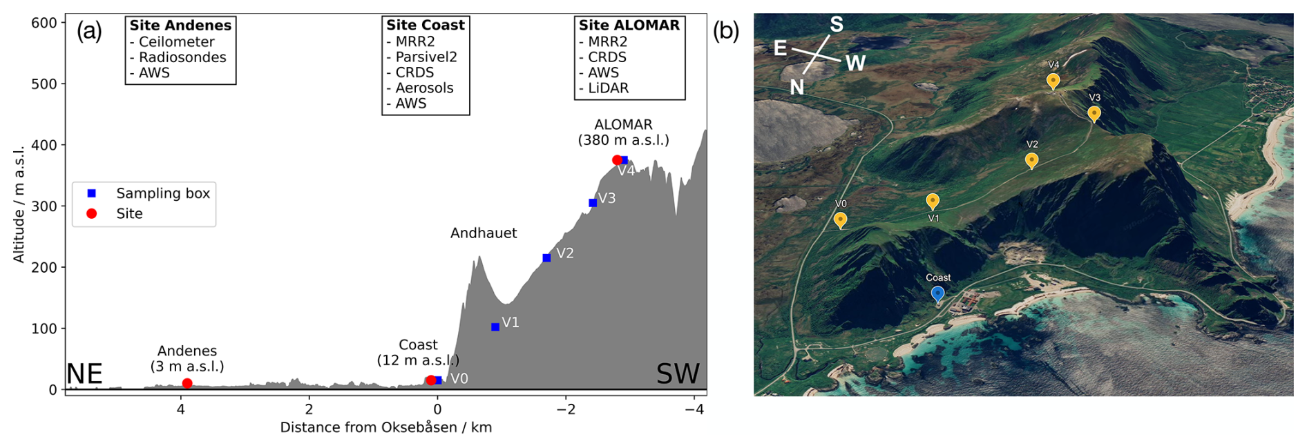
Figure 2 (a) Vertical cross-section of measurement and sampling setup at Andenes. Squares indicate the location of vertical transect sampling points. The sampling equipment installed along the transect is listed in top of the figure panel, for details see Table 1. (b) 3D view of topography around Andenes with site Coast and ALOMAR and location of sampling boxes for the vertical transect (Map data © 2025 Google).

Additionally, in order to assess the horizontal representativeness and spatial gradients in precipitation isotopes, precipitation sampling was performed along a 100 km-long surface transect from Andenes, reaching across the Vesterålen archipelago towards the South (Fig. 1b, Sect. 2.5). To further assess the horizontal variability in SWI signals, including the identification of Lagrangian matches during air mass transport, two additional water vapour isotope measurement sites were established in the town of Tromsø, Norway (120 km northeast of Andøya, Sect. 2.6) and in Bergen, Norway (1100 km southwest of Andøya, Fig. 1a, Sect. 2.7).

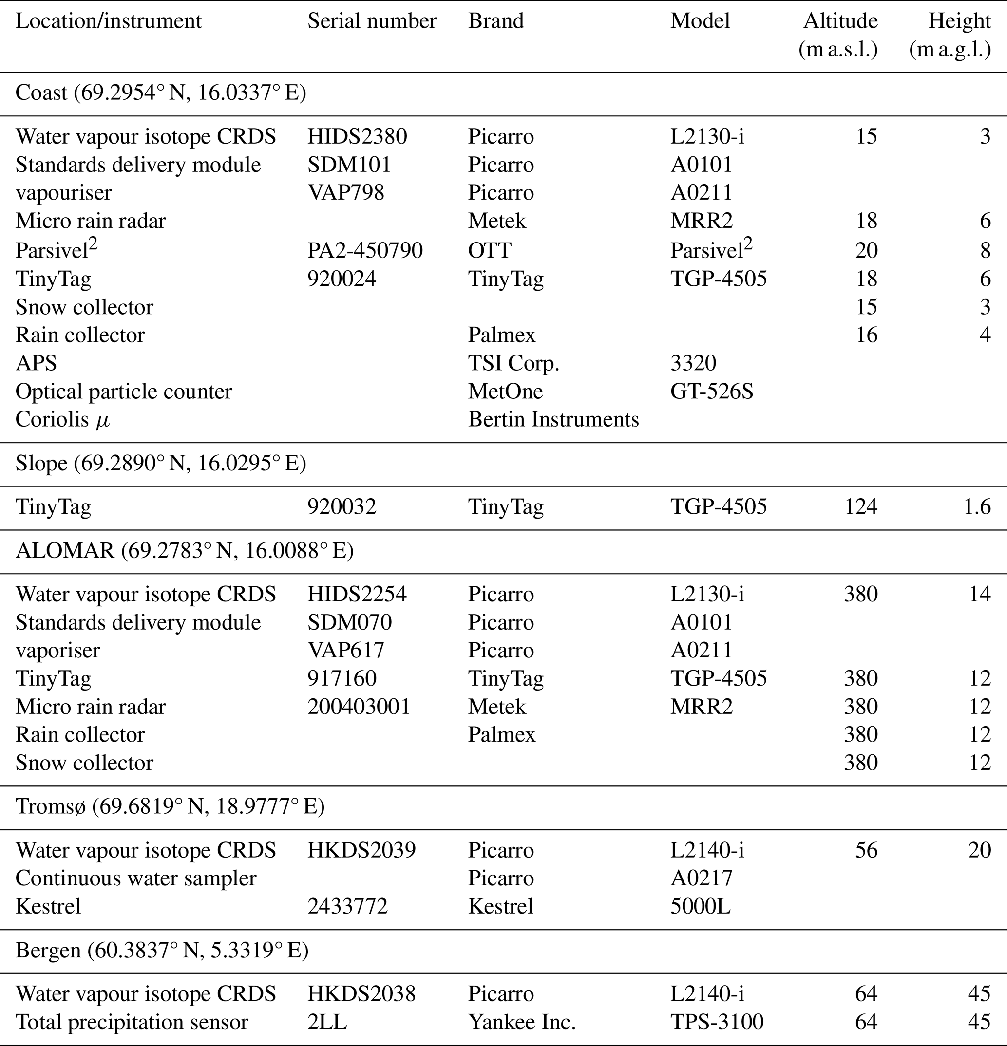
In addition to discrete sampling at regular intervals at the stations described above, higher-frequency sampling was conducted during intense observing periods (IOPs) depending on the prevailing meteorological conditions (Sect. 3.1). In the following sub-sections, we describe each of the sampling sites in more detail. The key measurement equipment used during the campaign at all locations is listed in Table 1, and the up-times and availability of the different datasets during the campaign are described in Sect. 3. The dataset for the individual types of measurements and sites is archived as a dataset bundle at https://doi.org/10.1594/PANGAEA.984616 (Sodemann et al., 2025).

Table 1 ISLAS2021 measurement instrumentation locations, instrumentation, and instrumentation metadata.

2.2 Instrumentation at site coast

2.2.1 Water vapour isotope measurements

Site Coast was set up to operate from 8 to 30 March 2021 near Andenes within a wooden building previously housing a lidar at the Oksebåsen premises of Andøya Space AS (Fig. A1). The measurement site was located 150 m south of the shore line, shielded to the south by a steep mountain slope rising to 288 m a.s.l.  Fig. 2a). At the building, a water vapour isotope analyser, a small automatic weather station (TinyTag), aerosol measurements, precipitation radar, and a drop size disdrometer were installed (Table 1). A CRDS (Cavity Ring-Down Spectrometer) water isotope analyser (L2130-i, Ser. No. HIDS2380, Picarro Inc., Sunnyvale, USA) was continuously measuring δD, δ¹⁸O and specific humidity in ambient air at a frequency of 0.8 Hz. Ambient air was guided to the stable water isotope analyser through a 4 m long $\mathrm{1}/\mathrm{4}$ in. stainless steel inlet, heated to 60 °C with self-regulating heating tape (Thermon Inc., USA), to avoid condensation and to reduce memory effects in the inlet line (Fig. A1b). The inlet line was flushed continuously at a flow rate of 5 L min⁻¹ with a manifold pump (N622, KNF GmbH, Germany). The inlet was installed on the north-east corner of the building at about 3 m above the ground. An inlet test showed a time delay of 18 s between inlet and the CRDS for mixing ratio and isotope species. A Standards Delivery Module (SDM, Part No. A0101, Picarro Inc., USA) and vapourizer (Part No. A0211, Picarro Inc., USA) were installed for calibration purposes, with dry air supplied from a molecular sieve (MT-400, VWR Inc., USA).

2.2.2 Aerosol measurements

Aerosol measurements were conducted using a separate 6 m long custom-made stainless-steel inlet, which was heated to ∼18 °C in order to ensure that rime and snow would not restrict the airflow through the inlet, and that hydrometeors were evaporated before entering the measurement equipment. At the base of the aerosol inlet, the flow was split between a series of aerosol counting and sizing instruments and a high-flow rate liquid impinger (Coriolis-μ, Bertin, France). The aerosol size distributions were measured by an optical particle counter (OPC, MetOne GT526S, UK) and an aerodynamic particle sizer (APS, TSI 3221, USA). The OPC was used to count and size particles with diameters above a certain size (i.e. 0.3, 0.5, 0.7, 1, 2, and 3 µm), while the APS counted particles between 0.7 and 20 µm in diameter in log-normal size bins.

As described in Gjelsvik et al. (2025), the Coriolis liquid impinger was used to collect and suspend aerosols in ultra-pure water (W4502-1L, Sigma-Aldrich, USA) for offline INP analysis. When the Coriolis was not sampling, an auxiliary blower (Model U71HL, Micronel AG, Switzerland) was connected to the airflow via a three-way ball valve (Model 120VKD025-L, Pfeiffer Vacuum, Germany) to maintain a 300 L min⁻¹ airflow through the inlet, similarly to Li et al. (2022) and Wieder et al. (2022). The Coriolis typically sampled for 40 min, resulting in 12 m³ of air sampled for each INP experiment. During the operation of the Coriolis, additional ultra-pure water was added to the sampling cone to offset evaporation with a typical pump rate of between 0.6 and 0.8 mL min⁻¹. The ice-nucleating ability of collected aerosols was assessed in situ using a drop-freezing technique DRoplet Ice Nuclei Counter Oslo (DRINCO) as described in Gjelsvik et al. (2025) and the cumulative INP concentrations were calculated following Vali (1971) (see Sect. 4.4).

2.2.3 Meteorological measurements

To characterize precipitation properties, a Micro Rain Radar (MRR2, Metek GmbH, Germany) and a laser disdrometer (Parsivel², OTT-Messtechnik GmbH, Germany) were installed on the roof of the wooden building at site Coast. The MRR is a vertically pointing K-band Doppler radar measuring reflectivity, drop size distributions, rain rate and liquid water content averaged over 10 s time intervals. The instrumental vertical range was configured to span from 100 to 3100 m with a 100 m vertical resolution. The Parsivel² disdrometer was used to obtain the size and fall velocity of hydrometeors. The hydrometeors were classified into 32 size and fall velocity classes. The Parsivel² instrument was configured to deliver all available measurement parameters at a 1 min time interval.

An ambient air temperature and relative humidity logger (Ser. No. 920024, TGP-4505), shielded by a small screen, was installed near the precipitation sensors for in situ meteorological observations, logging at a 2 min time interval. Furthermore, meteorological data were retrieved from a 108 m tall wind mast located 600 m to the south-west of the observational site (69.2937° N, 16.0191° E) hosted by Andøya Space AS. The mast provided measurements of air pressure, air temperature and relative humidity at 2 m height, as well as wind speed and wind direction at 18, 33, 48, 63, 78, 93, and 108 m, averaged to 10 s time resolution.

2.2.4 Precipitation and sea water sample collection

To collect precipitation samples for SWI analysis, snow and rain collectors were installed at the Coast building. Liquid precipitation was sampled using a rain collector (Palmex Inc., Croatia). The snow was collected in a clear plastic box with dimensions $\mathrm{40}\times \mathrm{30}\times \mathrm{32}$ cm (Fig. A2b). At the end of each sampling period, snow was mixed in the box with a plastic spoon and transferred to a sealable 68 mL PE bag (WhirlPak Inc., USA). Before sealing, extra air was squeezed out of the bag to reduce vapour exchange in the head space of the bag. The snow was melted in the bag at room temperature. For the analysis of INPs in precipitation, a total of 24 precipitation samples were collected in sterile 25 mL dispensing trays (613-1178, VWR, USA). For the SWI analysis, the collectors were exchanged with dry ones or dried with a paper towel before starting each new sample, while the dispensing trays for INP analysis were replaced after each precipitation sample. Both INP and SWI precipitation samples were taken at shorter time intervals during IOPs. In addition to vapour and precipitation measurements, daily coastal sea water samples were collected at 200 m from the site Coast at 1 m water depth. Samples were taken approximately daily, using 8 mL vials and sterile 50 mL Falcon Tubes (91051 TPP, Switzerland) for SWI and INP analysis, respectively (Gjelsvik, 2022).

For storage until SWI analysis in the laboratory, depending on the sample amount, rain, melted snow and sea-water samples were transferred after collection into 1.5 mL gas chromatography (GC) vials with open-top screw caps with PTFE/rubber septum, or into 8 mL vials with closed-top screw caps. Vials were stored upside-down at below 8 °C to minimise evaporation that would modify the isotope composition. The INP analysis was generally conducted immediately after collection (see Sect. 4.4). In some cases, the samples were stored frozen at −17 °C until analysis to prevent changes in the ice-nucleating ability of the collected samples (Stopelli et al., 2014; Beall et al., 2020).

2.3 Instrumentation at site ALOMAR

Site ALOMAR (Arctic Lidar Observatory for Middle Atmosphere Research) is an observatory located on the top of Ramnan Mountain at an elevation of 379 m a.s.l. and ∼3 km southeast of the town of Andenes, Norway (Fig. 2b). During the ISLAS2021 campaign, a water isotope CRDS analyser (L2130-i, Ser. No. HIDS2254, Picarro Inc., Sunnyvale, USA) was installed in the hatch control room on the roof top of the ALOMAR main building (Fig. A2). The analyser sampled ambient air from a 6 m long inlet line heated to 60 °C, that was flushed at a flow rate of about 5 L min⁻¹ by a manifold pump (N622, KNF GmbH, Germany), resulting in an average time delay before ambient signals arrived at the CRDS of about 20 s. The inlet was shielded from precipitation by a heated metal bowl, mounted at about 2.5 m above the platform level (385 m a.s.l. and 12 m a.g.l). During high wind speeds, snow could occasionally be lofted from surrounding structures and enter the inlet line, but would evaporate completely before reaching the analyser. An SDM (Picarro Inc., Sunnyvale, USA) and vaporiser (Part No. A0211, Picarro Inc., USA) were installed for calibration purposes. Dry air for the calibration vapour generation was produced from a molecular sieve (MT-400, VWR Inc., USA). Next to the inlet, a TinyTag logger (Ser. No. 917160, TGS-4505) with a small screen was installed to measure air temperature and relative humidity at a 2 min time interval.

Snow and rain samples were collected on the platform level at ALOMAR using a snow sampling box and a precipitation collector (Fig. A2b). Sampling frequency was increased during several IOPs (see Sect. 3.2). A rain collector (Palmex Inc., Croatia) was mounted to the railing close to the room housing the CRDS analyser. Data from a permanently installed MRR2 (Metek GmbH, Germany) were retrieved for the ISLAS2021 campaign period. The MRR was configured to report data at a 10 s time interval, with height bins from 35 to 1085 m until 14:30 UTC on 23 March 2021, and from 100 to 3100 m thereafter.

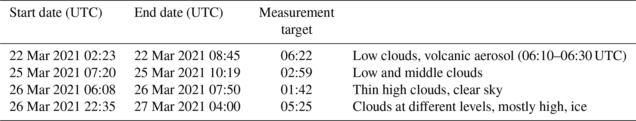
ALOMAR has been used for routine aerosol and cloud observations of the middle atmosphere since 1996 (Skatteboe, 1996) and for intensive measurement campaigns (e.g., Markowicz et al., 2012; Schäfer et al., 2022). During limited precipitation-free conditions, and in coordination with air traffic control from the nearby airport, the rooftop hatch was opened by an operator for lidar measurements (Fig. A2c,  Schäfer et al., 2022). The lidar utilised here is a system designed for measuring attenuated backscatter at three wavelengths (1064, 532, and 355 nm) and volume depolarisation ratio at one wavelength (532 nm) in the troposphere. lidar measurements were strongly constrained by the weather conditions, allowing for four valid measurement periods. The total duration of lidar measurements during the ISLAS2021 campaign was ca. 16.5 h, and contained high, middle and low clouds, periods of clear sky and volcanic aerosol, presumably from an ongoing Icelandic eruption (Table 3). Since operating the lidar required to open a large hatch of the ALOMAR building and the presence of an operator, measurements were limited to selected precipitation-free periods.

2.4 Instrumentation at site Andenes

Andøya meteorological station is located on the north-eastern part of Andøya island, 4.4 km from Andøya Space (69.3152° N, 16.1309° E, 3 m a.s.l., WMO-number: 1010). In addition to the near-surface measurements from an AWS, a ceilometer (CHM15k Nimbus, Lufft GmbH, Germany) obtained backscatter profiles and cloud layer heights continuously during the campaign. The ceilometer operates at a wavelength of 1064 nm and provides data with 15 s interval within an altitude range of 5 to 15000 m. Furthermore, an automatic sonde launcher at Andøya meteorological station released a total of 84 radiosondes between 23:03 UTC on 28 February and 17:03 UTC on 31 March 2021. Thereby, the regular twice-daily sounding interval (11:00 and 23:00 UTC) was increased to three to four times a day from 19 to 31 March 2021 (at approximately 05:00, 11:00, 17:00 and 23:00 UTC) during the ISLAS2021 campaign period.

2.5 Surface snow and precipitation sampling transects in Vesterålen

Surface snow and bulk precipitation were collected along a vertical transect between the sites Coast and ALOMAR (Fig. 2, blue boxes and yellow markers). Three sampling boxes (V1, V2, V3; Table 2) were placed between 100 and 300 m a.s.l. near the mountain road leading up to ALOMAR. One TinyTag (Ser. No. 920032, TGS-4505) was installed approximately half-way up along the slope of Ramnan mountain, near the site of box V2. The vertical profile was complemented by collection of surface snow at site V0 (25 m a.s.l.), and the regular precipitation collections at ALOMAR  V4) and Coast.

Table 2 Location of snow sampling boxes and sampling sites during ISLAS2021.

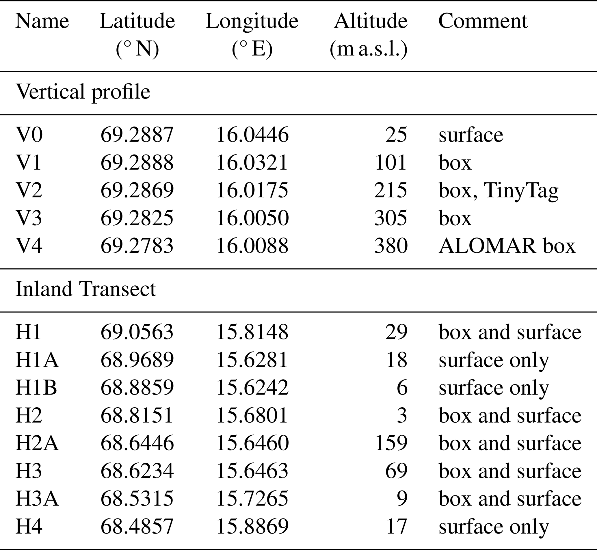
Table 3 Overview of measurement periods and respective targets of the aerosol lidar at ALOMAR during the ISLAS2021 campaign. Since the main hatch of the building had to be opened to operate the lidar, measurements were only possible for sufficiently long precipitation-free periods.

Precipitation and surface snow were also collected along a horizontal transect from Andenes across Vesterålen towards the Norwegian main land. In total 5 sampling boxes (H1, H2, H2A, H3, H4) were installed for bulk precipitation sampling. Snow surface samples were collected at sites H1 to H4 as well as at four additional locations (H0, H1A, H1B, H3A, Fig. 1b). The locations cover a distance of approximately 100 km from the north coast of Andøya to the south coast of Hinnøya, with the aim to identify potential isotopic signals from isotopic distillation across the coastal mountains, and to quantify the spatial representativeness of precipitation isotopes measured at Andenes. Boxes were placed in an open area or on the upper part of a sloping area to minimise the collection of blowing snow.

At each location, box samples (consisting of solid or liquid precipitation, or a mixture) were collected using sampling bags and a plastic spoon as described in Sect. 2.2. After sample collection, the boxes were emptied and dried with a paper towel. When solid precipitation had accumulated since the previous visit, additional surface snow samples were collected with a spoon and sampling bag from a location within a few metres of the box. At locations H0, H1A, H1B and H3A, only surface snow samples were collected. Boxes H1, H2, H3, and H4 were installed on 18 March and H2A on 23 March 2021. Boxes were if possible cleared ahead of a new IOP to obtain a clean signal without drifting surface snow. The sampling interval and potential for resulting post-depositional effects are described in Sect. 3.2. On several occasions, a small meteorological probe (iMet XQ-2, InterMet systems Inc., USA) was mounted outside a car window to obtain horizontal transects of air temperature and relative humidity between Andenes and the horizontal transect sites.

2.6 Instrumentation at site Tromsø

One set of water vapour isotope measurement equipment was originally planned to be installed on a research vessel for underway sea water and water vapour measurements. However, sanitary restrictions due to COVID-19 required on short notice to repurpose the instrumentation to a land-based water vapour measurement station. As an alternative measure, a water vapour isotope measurement station was set up at the town of Tromsø, located ∼120 km to the north-east of Andenes (Fig. 1b). Situated on an island in the fjord Straumsfjorden, the town is shielded from the open ocean to the west and north by mountains with elevations exceeding 1000 m. An ambient air inlet, protected with a heated precipitation shield was installed at 56 m a.s.l. on the roof of Natural Science building of the University of Tromsø (UiT, 69.6819° N, 18.9777° E), near a web camera and AWS owned by UiT (Fig. A3b, blue square). The inlet line (ca. 6 m PTFE) was heated to 60 °C with self-regulating heating tape (Thermon Inc., USA) and flushed continuously with an inlet pump (N622, KNF GmbH, Germany). A portable weather station (Kestrel 5000L, Nielsen-Kellerman Co., USA) was installed near the inlet on the roof (Fig. A3c). The indoor installation was set up in a rooftop instrument room, and consisted of a water vapour isotope analyser (L2140-i, Ser. No. HKDS2039, Picarro Inc., USA) and a Continuous Water Sampler (CWS, Part No. A0217, Picarro Inc., USA) used here for instrument calibration. After setup, the analyser by mistake partly sampled room air through an open split connecting the CWS and the Picarro in the first half of the campaign (until 20 March 2021). On 21 March 2021, the leak was fixed by disconnecting the CWS. The CRDS analyser thereafter continuously sampled air from the flushed inlet line.

2.7 Instrumentation at site Bergen

Another sampling station was set up in the city of Bergen, located in the south-western part of Norway (Fig. 1). While Bergen is generally more influenced by mid-latitude weather systems, the site was located either upstream or downstream of the sampling sites in Northern Norway on several occasions. Continuous water vapour isotope measurements during the campaign were performed at the roof of Geophysical Institute, University of Bergen (60.3837° N, 5.3319° E, 56 m a.s.l.) using the setup described in Weng et al. (2021). In short, a CRDS analyser (L2140-i, Ser. No. HKDS2038, Picarro Inc., Sunnyvalye, USA) continuously sampled from a heated inlet (60 °C) shielded from precipitation at the instrument tower of the building, and flushed with a flow rate of 5 L min⁻¹ by a manifold pump (N622, KNF GmbH, Germany). Measurements of air temperature, relative humidity, pressure and total precipitation close to the air inlet were performed using a hotplate pluviometer (TPS-3100, Yankee Inc., USA) and an AWS (Anderaa, Norway).

In addition, measurements of air temperature, relative humidity, and precipitation were provided by the AWS Bergen-Florida (WMO-number 1317), located at 16 m a.s.l. in the garden of the Geophysical Institute. Previous studies showed that the precipitation measured by the rain gauge at the AWS is ∼10 % lower than measured by the pluviometer at the tower (Weng et al., 2021). Precipitation sampling for SWI analysis was conducted during the ISLAS2021 campaign at a location 1.3 km north-east of the Geophysical institute (60.3872° N, 5.3537° E, 143 m a.s.l.) with a manual rain collector for event-based sampling.

3 Campaign implementation

This section describes the weather conditions encountered during the active measurement period from 15 to 30 March 2021, and gives an overview over the uptimes of different instrumentation, discrete sample collection, and the in-total eight IOPs during the campaign.

3.1 Meteorological conditions during the campaign

We now first describe the general weather conditions encountered during the campaign. The measurement period of the ISLAS2021 campaign was characterised by large synoptic variability. A general classification into weather events associated with warm-air advection from mid-latitudes, and cold-air advection from the Arctic was employed to distinguish between different IOPs (Table 4). A positive CAO index, defined as the difference between the potential temperature at sea level and at 850 hPa is used to delineate regions dominated by arctic air masses, and associated with large heat fluxes (Papritz and Spengler, 2017; Geerts et al., 2022). We use the percent area coverage with positive mCAO conditions in two domains, a box just offshore of Andenes (69–70° N, 14–17° E), and a larger box including the Vesterålen archipelago and Tromsø (67–70° N, 12–20° E), to quantify regional mCAO conditions near the sampling sites (Fig. 3c, black and cyan lines). Sea level pressure (SLP), wind speed, and precipitation rate further illustrate the synoptic variability (Fig. 3a and b).

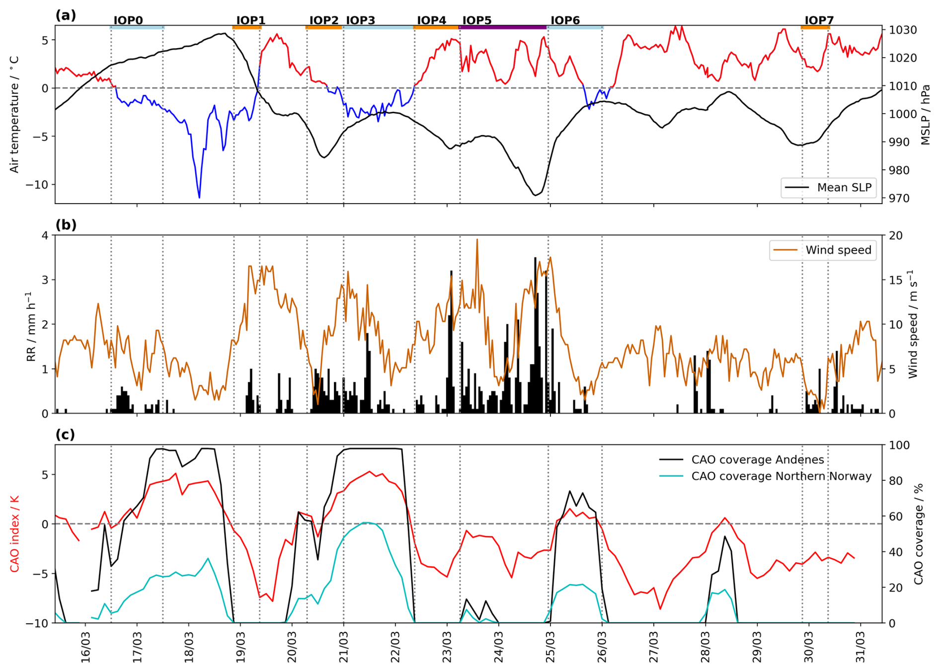
Figure 3 Weather evolution during the ISLAS2021 campaign. (a) Air temperature (°C, red/blue) and mean SLP (hPa, black) at Andøya WMO station. (b) Precipitation (mm h⁻¹, black bars) and wind speed (m s⁻¹, orange line) recorded at Andøya WMO station. (c) CAO index calculated from AROME-Arctic forecast data for Andenes (red line, K), and area coverage with CAO index above 2 K for a domain near Andenes (69–70° N, 14–17° E, %, black line) and a larger domain in Northern Norway (67–70° N, 12–20° E, %, cyan line). The grey vertical dashed lines mark different IOPs labelled on top (orange: WAIs, cyan: mCAOs, purple: cyclone).

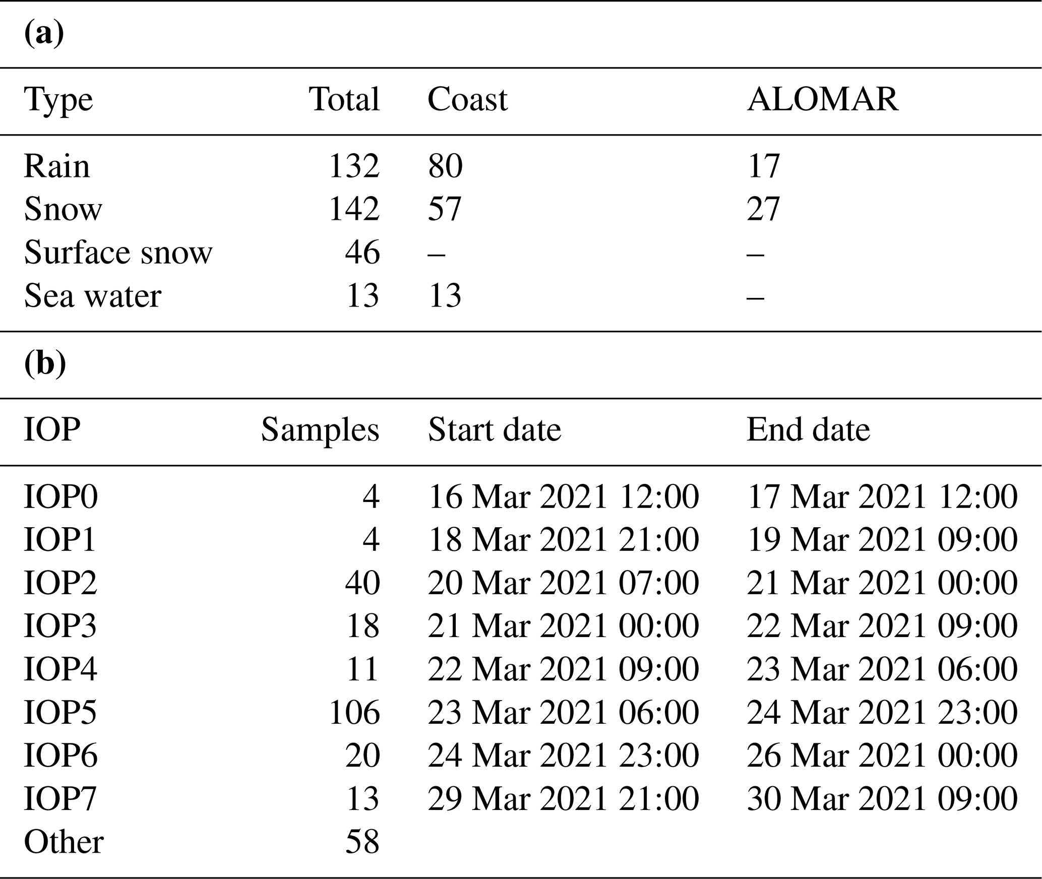
Table 4 Number and type of discrete water samples taken during the ISLAS2021 campaign. (a) Summary of sample types taken from different water cycle components at key sites. (b) Samples taken during the Intense Observation Periods (IOPs).

The first IOP, termed IOP0 since it took already place before all instrumentation was completely operational, lasted from 16 to 17 March 2021. At that time, a mCAO extended from the Barents Sea towards Andenes (not shown). During IOP0, the coldest air temperatures in Andenes during the measurement campaign were observed (below −11 °C; Fig. 3a) and the CAO index reached 5.1 K (Fig. 3c, red line). A high-pressure system over Svalbard and the Norwegian Sea directed the flow of arctic air towards Andenes (Fig. 4a). The high-pressure system subsequently moved eastward during IOP1 (18 to 19 March 2021), and a large mid-latitude cyclone moved into the Norwegian sea, with its core marked by integrated water vapour above 8 kg m⁻² east of Svalbard (Fig. 4a, shading). At that time, the CAO index had decreased, and precipitation from the warm sector of this system reached Andenes (Fig. 3b and c). During IOP2, a rapid passage of narrow fronts associated with a short-wave system originating over Greenland occurred within 24 h, as seen from the minimum in SLP on 20 March 2021 of about 988 hPa (Fig. 3a, black line).

The most pronounced mCAO both in spatial coverage and CAO index magnitude (maximum value was 5.3 K) was encountered during IOP3 from the 21 to 22 March 2021 (Fig. 3c). Intense showers, wind gusts, and temperature variations were observed as individual convective cells passed over the observing site Coast during that period (Fig. 4c). IOP4, starting on 22 March 2021, was associated with the passage of a large frontal system that progressed poleward into the Barents Sea (Fig. 4d). This IOP4 was characterised by warmer air temperatures of up to 5 °C, intense precipitation of up to 3 mm h⁻¹, and a lower CAO index (Fig. 3a and b). As the mid-latitude cyclone had moved poleward, an intense cyclone developed on the trailing system. During IOP5 on 23–24 March 2021, the site Coast was hit directly by the rapidly intensifying cyclone (“atmospheric bomb”), reflected in a minimum SLP of 970 hPa (Fig. 4e). This event was associated with the largest accumulated amount of precipitation during ISLAS2021, and winds of up to 20 ms⁻¹ at site Coast (Fig. 3b). As the cyclone moved away towards the east, it gave way to colder air reaching Andenes, initiating IOP6 that was associated with a short period of mCAO conditions with convective cells and snow showers (Fig. 4f). During IOP7 on 29 March 2021, a mesoscale cyclone moving northward along the coast of Norway brought warm air masses and light rain to Andenes from its narrow frontal band (Fig. 3c).

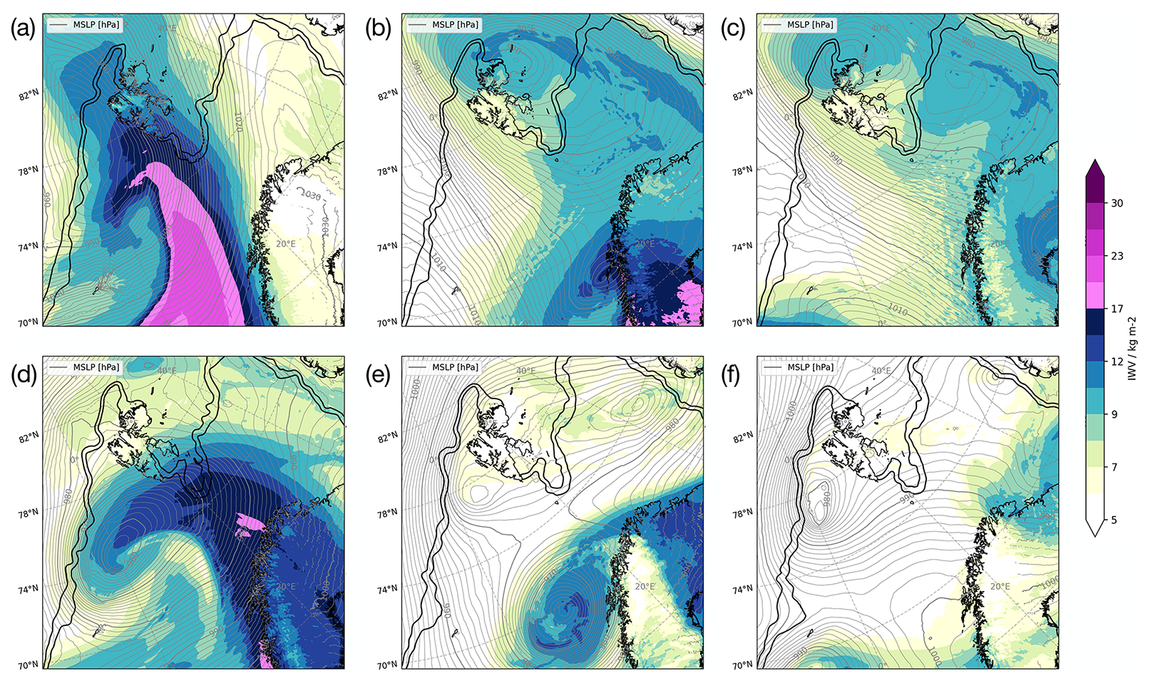
Figure 4 Weather situation according to operational forecasts from AROME-Arctic in terms of SLP (grey contours) and vertically integrated water vapour (shading) during IOPs 1 to 6. (a) IOP1 (12Z on 17 March 2021), (b) IOP2 (12Z on 17 March 2021), (c) IOP3 (12Z on 21 March 2021), (d) IOP4 (12Z on 17 March 2021), (e) IOP5 (12Z on 25 March 2021), and (d) IOP6 (12Z on 28 March 2021). Black solid lines denotes model-predicted 80 % and 90 % sea ice concentration.

3.2 Data acquisition and data availability

With the first installations starting on 15 March 2021 at Tromsø and site Coast, the continuous measurements became operational across all sites on 16 March (Fig. 5a). The CRDS analysers did not record ambient vapour measurements during daily calibration periods. The CRDS analyser in Tromsø partly sampled room air in the period 15 to 23 March 2021, leading to a strongly muted signal of ambient-air isotope variations (light red shading). As no personnel was present in the room during the measurement period, and a ventilation provided continuous exchange of ambient air into the room, we decided to retain the time period as part of the dataset, but denoted with a quality flag. During 28 to 30 March 2021, the analyser did not record measurements. The CRDS at site Coast was disconnected from its inlet for performance tests during 26–27 March 2021. Data from the MRR at ALOMAR became available at 100 m vertical resolution during 19 March 2021, changing from 35 m vertical resolution before. The MRR at Coast, the Parsivel² disdrometer and the ceilometer delivered data throughout the campaign except for a few short interruptions. Disassembly started on 30 March 2021, and was completed during the following day.

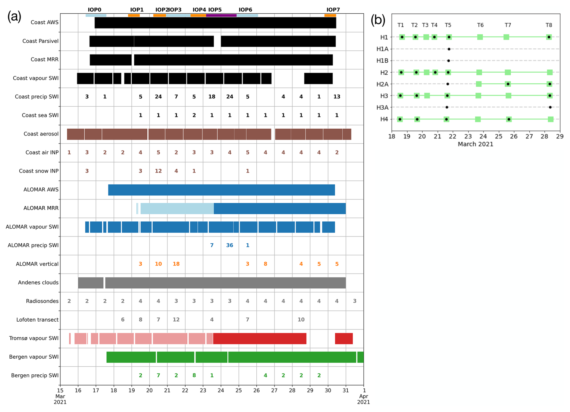
Figure 5 Data availability chart for continuous and discrete measurements of the ISLAS2021 dataset. (a) Measurement up times for instrumentation at the various campaign locations and number of collected samples. Light blue shading indicates limited vertical resolution for the ALOMAR MRR at the start of the campaign. Light red shading indicates measurement of room air at the CRDS installed in Tromsø. (b) Horizontal transect sampling during the campaign period. Green squares denote sampling boxes, black dots are surface snow samples.

Across the measurement network, at least two CRDS were operating during 99.2 % (158.8 h) of the campaign duration of 160.1 h, at least three analysers were measuring during 85.7 % (137.2 h), and all four analysers were operating during 23.5 % (37.6 h). When including the period of the inlet leakage in Tromsø as measurement time in the calculation, the percentage when all four CRDS were measuring increases to 58.3 % (93.2 h). The most complete coverage of isotope measurements was obtained from 23 to 27 March 2021. The opening of the lidar hatch at ALOMAR, that was located approximately 5 m away from the inlet, did not produce a measurable imprint on the water vapour isotope signal. From regular and additional radiosonde launches, a total of 57 balloon ascents are available during the campaign period. The radiosondes measured wind speed and direction using GPS, as well as air pressure from a silicon capacitor, air temperature from a resistive sensor, and relative humidity from a humicap sensor. All data is reported at a 2 s time interval.

Discrete sampling of precipitation, and other discrete measurements, were organised into the sequence of IOPs corresponding to pronounced changes in the prevailing meteorological conditions (Sect. 3.1 and colour bars on top of Fig. 5a). The total of 137 precipitation samples taken at site Coast were collected mainly during IOPs 3, 4, 5, and 7 (Table 4b). Precipitation at site ALOMAR was only collected at high resolution during IOP4 and IOP5. The total of 56 precipitation samples from 8 vertical transects from the boxes and locations V0 to V4 were mostly from IOP3. A total of 54 precipitation samples were collected on the 8 horizontal transects (T1–T8, Fig. 5b). The typical duration until sampling was 1 d or less for Transects T2–T5, and two days or more for T6–T8, increasing the potential for post-deposition effects to modify the precipitation signature. The most detailed horizontal and vertical sampling was carried out during IOP3 (Transect T5). The severe weather during IOP5 only allowed for collection of the total precipitation from the horizontal transect at the end of the event (T7). Bergen precipitation (30 samples) was collected mostly on a daily basis, but also included higher frequency sampling when the mCAO of IOP3 arrived in Bergen on 22 March 2021. Sea water was collected on a daily basis, except for two samples collected on 22 March 2021, providing a total of 13 samples. INPs were analysed for 52 precipitation samples, up to 5 times per day.

4 Processing, calibration, and laboratory analysis

This section details the calibration and processing of water vapour isotope measurements during the campaign, as well as the laboratory analysis and processing of discrete samples of precipitation, surface snow, sea water and aerosols.

4.1 Processing and calibration of water vapour isotope measurements

Water vapour isotope measurements from all analysers were processed with an overall similar routine with small specific adjustments. First, raw isotope measurements were corrected for the mixing ratio–isotope ratio dependency of each specific analyser using a correction curve determined in the laboratory (Weng et al., 2020; Sodemann et al., 2023b). The CRDS analyser at site Coast suffered from unusually strong mixing ratio–isotope ratio dependency, which was corrected using the dependency presented in Appendix C. Next, data was normalised to VSMOW-SLAP scale using long-term calibration coefficients specific to each analyser, as described in Appendix B and the following paragraphs. The calibrated water vapour isotope data, along with ambient pressure, water vapour mixing ratio, and several instrument parameters were then averaged (5 min time resolution for site Coast, 2  min for site ALOMAR and Tromsø, 10 min for site Bergen), and combined with the corresponding meteorological measurements from meteorological sensors mounted near the inlets. Specific humidity calculated from the meteorological data was thereby used to time-reference the CRDS measurements.

The CRDS analysers installed at ALOMAR, Tromsø, and in Bergen were each calibrated using instrument-specific long-term calibration coefficients (Table B1). These coefficients were obtained from repeated measurements of known secondary standards normalised to VSMOW-SLAP scale over at least several months from a combination of SDM and liquid injection measurements in a controlled laboratory environment. On-site calibrations during the campaign were used to check the validity of the calibration line in terms of slope and offset of the calibration curve. The rationale behind this approach to calibration rather than, e.g., interpolating from one calibration to the next within a measurement interval of 23 h, is that uncertainty introduced by the calibration system in a field setup is similar to the analyser uncertainty, for example due to less reliable dry air provision to calibration units. In addition, the same type of analyser as used here has been observed to have negligible drift over months up to years (Bailey et al., 2023; Seidl et al., 2026). The field calibrations are then used as part of calculating the combined uncertainty (see Sect. 4.2). For the CRDS at site Coast, no reliable long-term calibration had been established at the time of the campaign, and the water vapour isotope measurements were therefore calibrated using the average of all available calibrations during the campaign period.

More specifically, for the CRDS analyser installed at ALOMAR (Ser. No. HIDS2254), calibration checks were performed daily with two secondary standards (Table D1, DI and GSM1). Due to the standard bag being almost empty, standard GSM1 was replaced by standard GLW on 17:15 UTC on 21 March 2021. Drift was less than or smaller than the uncertainty of the calibrations. The CRDS analyser at site Coast (Ser. No. HIDS2380) was calibrated at a 23 h interval using standards EVAP2 and GLW. The CRDS analyser in Tromsø (Ser. No. HKDS2039) was calibrated using a CWS. The CWS was used, since the analyser originally was intended to be deployed on a research vessel. Calibrations were performed daily except for the period of 24 to 30 March 2021 when the CWS was disconnected. Thereby, the CWS supplied three secondary standards in the sequence DIX, GLX and MYRK for 20 min each, with the last 10 min being retained. While the mixing ratio of the retained periods was sufficiently stable (standard deviation between 56 and 346 ppmv), the average humidity of each calibration step varied, requiring correction using linear isotope-humidity dependency derived for this specific analyser. Drift was smaller than calibration uncertainty. The CRDS analyser in Bergen (Ser. No. HKDS2038) was calibrated using four to six manual injections of secondary standards DI2 and GLW at five days during the campaign period. The average of the last three satisfactory injections confirmed consistency with the long-term calibration parameters.

4.2 Uncertainty budget of water vapour isotope measurements

To compute the uncertainty budget for vapour isotope measurements, we adopt here an approach that is also commonly used for liquid water sample isotope analysis (Gröning, 2011; Sodemann et al., 2023b). The combined uncertainty is thereby obtained from the squared sum of calibration standards uncertainty, the uncertainty field calibration, and the uncertainty of the sample measurements, each weighted by the sensitivity to the calibration slope. Thereby, the uncertainty of each sample measurement is estimated from the standard deviation during an averaging interval (Eq. D3). Since the CRDS at site Coast had an about four times larger standard deviation for both isotopes than the other CRDS, a 24-point moving average (corresponding to a ∼20 s time window) was applied to the δ¹⁸O and δD measurements, before recalculating the d-excess. While some finer-scale structures where thus lost from the time series, this filtering brought the estimate of the measurement uncertainty to a range comparable to the other analysers.

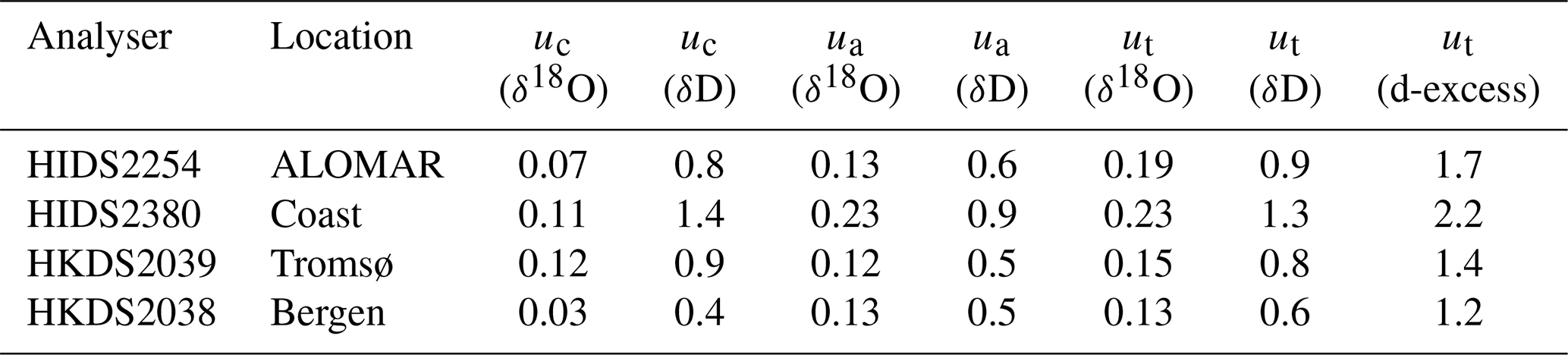
Components of the uncertainty budget for the four CRDS analysers are summarised in Table 5. The uncertainty of the calibration standards can be retrieved from Table D1. The combined (total) uncertainty u_t presented here is calculated for an the average isotope composition and mixing ratio over the entire field period. Uncertainty will increase with lower mixing ratio (larger analytical uncertainty) and towards the upper and lower end of the calibration curve (sensitivities). The uncertainty budget is generally dominated by the measurement uncertainty (35 %–90 %), while analytical uncertainty is largest for sites Coast and Tromsø (∼20 %–40 %, not shown). It should be noted that the combined uncertainty of the d-excess is ∼2 ‰ãcross all sites. Together with the use of common reference standards and processing steps, this enables meaningful comparisons across the CRDS network. In addition, a bias correction was required for the CRDS at site Coast, as detailed in Sect. 5.1.

Table 5 Uncertainty budget components for the four CRDS analysers for water vapour isotope analysis deployed during the ISLAS2021 campaign. u_c: uncertainty of calibrations (‰), u_a: analytical uncertainty (‰), u_t: total (combined) uncertainty (‰). The total uncertainty for analyser HIDS2380 includes also a bias correction uncertainty of 0.06 ‰.

4.3 Laboratory analysis and calibration of precipitation and sea-water samples

The freshwater (rain, snow and surface snow) and seawater samples were analysed at The Facility for Advanced Isotopic Research and Monitoring of Weather, Climate and Biogeochemical Cycling (FARLAB) at the University of Bergen. Prior to analysis, the samples were filtered and transferred to 2 mL GC-vials (ThermoSci 2-SVW Chromacol). Analysis procedures followed the scheme utilised at FARLAB described in Sodemann et al. (2023a). In short, each batch of about 20 samples was supplemented with secondary laboratory standards DI2, GLW, FIN and EVAP2 in use at FARLAB, which had been calibrated to the VSMOW-SLAP scale against primary standards available from the International Atomic Energy Agency (Table D1). Similarly to the procedure described in Weng et al. (2021), 12 injections and 6 injections were done for each standard and sample, respectively. For the sea water samples, a salt liner was installed in the vaporiser. During the run, the water was transferred from the vials to the vaporiser using an autosampler, and high-purity-grade N₂ (nitrogen 5.0, purity > 99.999 %; Praxair Norge AS, H₂O mixing ratio < 5 ppmv) was used as matrix gas.

After the analysis, each run was calibrated and corrected for memory effects and isotope ratio–mixing ratio dependency corrections for each individual analyser using the software FLIIMP (FARLAB liquid water isotope measurement processor Sodemann et al., 2023a). Samples were corrected for drift and memory, and normalised for VSMOW-SLAP scale using laboratory standards. The uncertainty of the calibrated samples is calculated based on the assigned uncertainty of the isotopically heavy and light standard with respect to VSMOW-SLAP, the uncertainty of measured values of the standards, and the uncertainty of the sample approximated by the standard deviation of repeated measurements or by long-term reproducibility. Long-term reproducibility at FARLAB for measurement of drift standard DI2 has been estimated to 0.052 ‰ for δ¹⁸O and 0.446 ‰ for δD, respectively (Sodemann et al., 2023a).

4.4 Processing of aerosol samples

After collection of aerosol samples at the site Coast, the ice-nucleating ability of aerosols was quantified in situ using the home-built drop freezing setup DRINCO (Gjelsvik et al., 2025), based on the design of David et al. (2019) and Miller et al. (2021). DRINCO uses a webcam to monitor the freezing of 50 µL aliquots of sample pipetted into a 96-well PCR tray that is partially submerged in a temperature controlled ethanol bath (FP51, Julabo). The webcam captures the freezing progression of the aliquots at 0.25 °C intervals while the ethanol bath is cooled at a rate of 1 °C min⁻¹. An aliquot is identified as frozen based on the amount of light that is transmitted through a well, with a sharp decrease in light transmission after freezing due to the enhanced light scattering in ice relative to water. The result of the experiment is a frozen fraction (FF) for each 0.25 °C interval between −30 and −2 °C. The frozen fraction was then converted to an INP concentration per temperature (INP_air(T)) using Poisson counting statistics described by Vali (1971) and calculated as:

$$\begin{array}{}\text{(2)}& {\mathrm{INP}}_{\mathrm{air}}\left(T\right)={\displaystyle \frac{-\ln (\mathrm{1}-\mathrm{FF}(T\left)\right)\cdot V_{\mathrm{sample}}}{V_{\mathrm{droplet}}{V}_{\mathrm{air}}}},\end{array}$$

where V_droplet is the size of the aliquot in each well (50 µL), V_sample is the volume of water in the Coriolis sampling cone at the end of the sampling period and V_air is the volume of air sampled by the Coriolis during the sample.

All of the aerosol and INP concentrations were normalised to (std L)⁻¹ by using the inlet temperature as measured and recorded by a Type K thermocouple and datalogger (EL-GFX-TC, Lascar Electronics datalogger), respectively, and ambient pressure measurements from the Norwegian Meteorological Institute site located in the town of Andenes (see Sect. 2.4).

When accounting for the 12 m³ of air sampled with the Coriolis impinger (Sect. 2.2.2) and a residual cone volume of approximately 15 mL, the minimum detection limit of INPs was $\sim \mathrm{2.5}\times {\mathrm{10}}^{-\mathrm{4}}$ std L⁻¹ at temperatures warmer than −17 °C. Due to the low-end cutoff size of the Coriolis (∼0.5 µm), it is expected that the INP concentration reflects both biological and mineralogical INPs that are typically larger than this size.

5 Campaign datasets

This section describes the data collected during the campaign, provides insight into important dataset limitations and uncertainties, and presents examples for data usage.

5.1 Water vapour isotope measurements across the network

Within the ISLAS2021 campaign setup, a network of stable isotope analysers was deployed on distances of a few km (sites Coast and ALOMAR), to 120 km (site Tromsø), to 1100 km (site Bergen). If the analysers are calibrated consistently, covariances, offsets, and time shifts between the different sites can be interpreted in terms of processes and meteorological influences, and thus inform about spatial representativeness of this kind of measurements. The specific humidity from sites Coast (Fig. 6a, black line) and ALOMAR (blue line) shows a very large degree of similarity throughout the campaign. There are a few occasions during IOP1, IOP4 and IOP6 where site Coast appears to encounter drier conditions. The specific humidity at Tromsø (red line) still appears similar, for example during IOP5, but also has periods with large differences (e.g., more humid during IOP6), in line with expectations for the larger distance between sites. Specific humidity at site Bergen is substantially higher throughout the campaign (Fig. 6a, green line), except for short periods after IOP1, at the start of IOP3, and on 28 March 2021. While possibly coincidental, some of the increases and decreases appear to lead or lag compared to the measurements from Northern Norway. Detailed trajectory analysis in forthcoming studies will enable identification of any Lagrangian matches between Bergen and Andenes during this period.

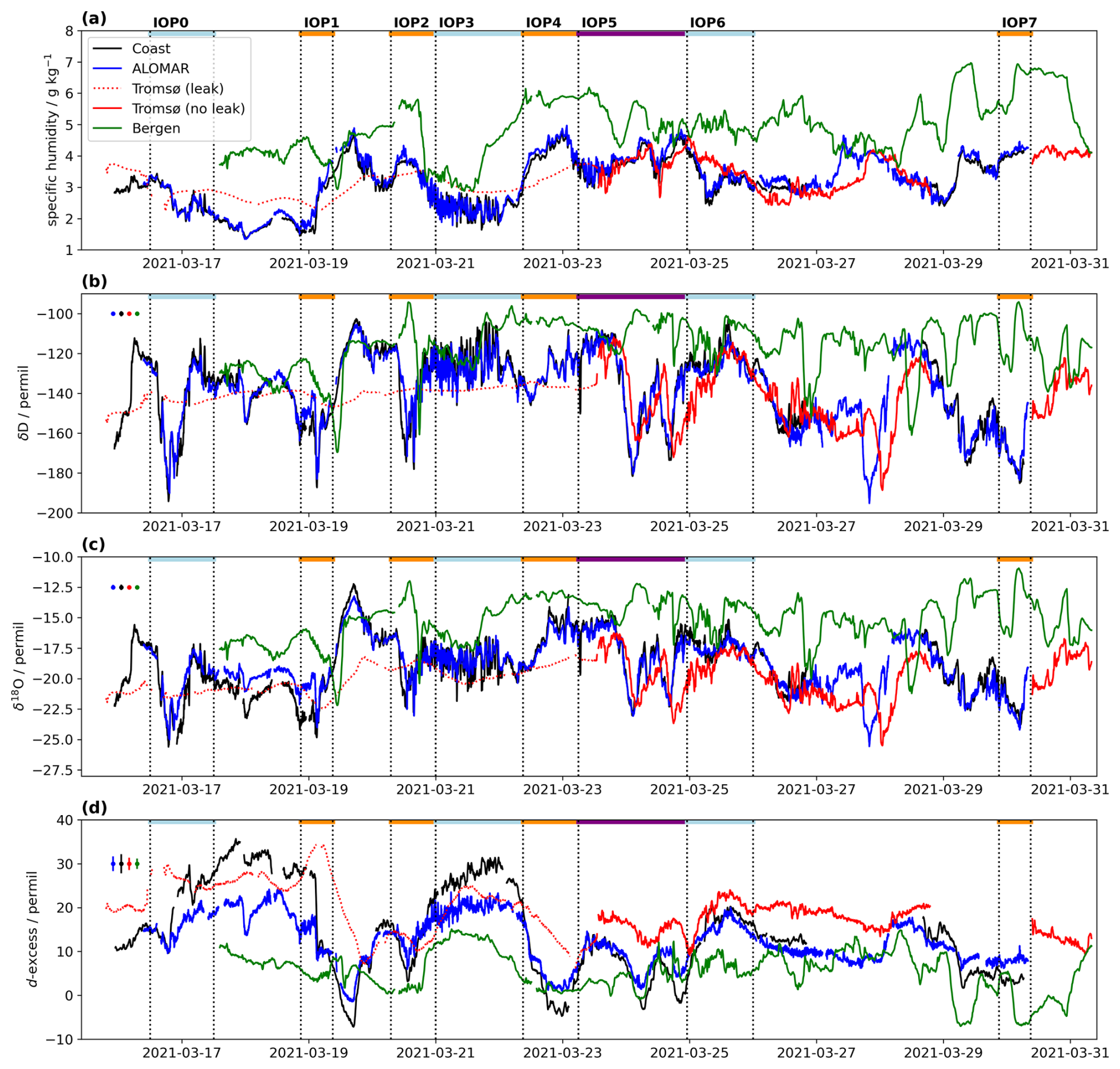
Figure 6 Time series of water vapour and water vapour isotope measurements from the CRDS network at site Coast (black line), ALOMAR (blue line), Tromsø (red line), and Bergen (green line) during ISLAS2021. (a) Specific humidity (g kg⁻¹), (b) δD (‰), (c) δ¹⁸O (‰), (d) d-excess (‰). Measurements from Tromsø station are affected by a leak of room air before 12:00 UTC 23 March 2021 (red dotted line). Error bars on the left indicate the total uncertainty for each CRDS analyser at the average mixing ratio and isotope composition at each location during the campaign. Blue, orange and purple bars at the top of panel (a)–(d) denote IOPs.

Variations in specific humidity at the sites Coast, ALOMAR and Tromsø were also frequently reflected in the δD (Fig. 6b). During some episodes, there were marked deviations from this rule, such as during IOP5 (purple bar), where δD dropped markedly. Furthermore, offsets between Tromsø and the Andenes measurements become apparent in δD, again during IOP5 (23–24 March 2021) and during 27 March 2021, with Tromsø lagging by 3–6 h. Another interesting observation is that δD measured in Bergen co-varied with the other sites during some periods, such as parts of IOP1, IOP2 and IOP3, despite the more humid conditions. In these situations, the isotopic signal may contain information about distillation or evaporation effects during the ∼1000 km long transport path.

The δ¹⁸O in general shows a very similar relation between all sites as δD (Fig. 6c). However, the site Coast was on average 1.65 ‰ more depleted than site ALOMA ‰. Given the large correction for mixing ratio dependency that had to be applied to the δ¹⁸O, and the larger measurement uncertainty of that particular analyser, several lines of evidence were investigated to identify if this bias was real or an artefact of the calibration procedure. Computing the d-excess from the measurements, the site Coast would at times reach 52.1 ‰, with an average of 27.5 ‰. All other sites only reached a d-excess of up to 24.2 ‰ (ALOMAR), 34.3 ‰ (Tromsø), and 15.1 ‰ (Bergen). Furthermore, correspondence to the GMWL was investigated in a δD–δ¹⁸O correlation plot (Fig. 7a). Periods with high d-excess were far from equilibrium, and would have to have evaporated from very low relative humidity with respect to sea surface temperature. Even though it may be plausible to expect a higher d-excess at site Coast, which is closest to evaporation conditions, an overall lower δ¹⁸O than at ALOMAR, but a higher δD, was deemed implausible given the large correction of the raw δ¹⁸O measurement signal. Therefore, the median offset between site ALOMAR and Coast was calculated for the entire campaign, and then used to bias correct the δ¹⁸O of site Coast by 1.65 ‰ (Fig. 6b, black line). The uncertainty of the bias was estimated as 0.06 ‰, using the squared sum of the standard error of the mean scaled by $\sqrt{\mathit{\pi }/\mathrm{2}}$ for all δ¹⁸O measurements at ALOMAR and Coast, respectively. Combining the bias uncertainty with the total analytical uncertainty changed the final uncertainty estimate only marginally from 0.22 ‰ to 0.23 ‰ (Table 5). The dataset on the data repository already includes the bias correction, such that it does not need to be applied by the data users.

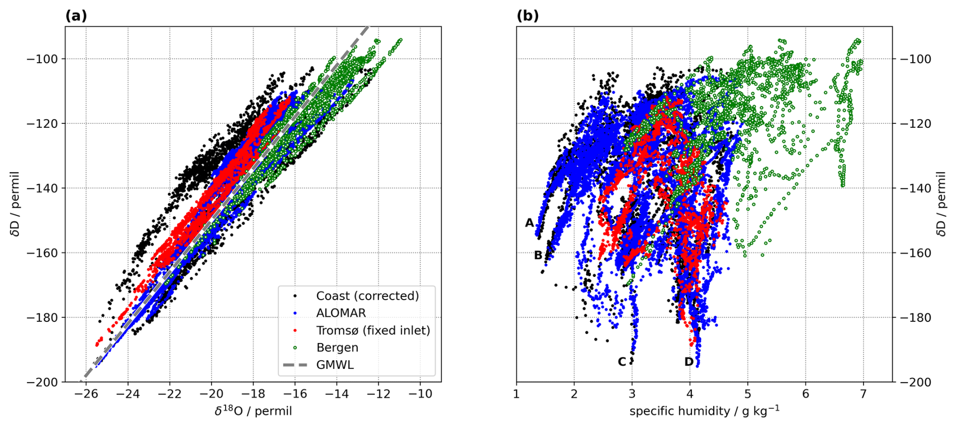
Figure 7 Summary characteristics of all (high-quality) water vapour isotope measurements from the CRDS network during ISLAS2021. (a) Comparison of the δD-δ¹⁸O correlation in water vapour isotope measurements from site Coast (black dots), ALOMAR (blue dots), Tromsø (red dots), and Bergen (green dots) compared with the Global meteoric water line (GMWL, $\mathit{\delta }\mathrm{D}=\mathrm{8}\times {\mathit{\delta }}^{\mathrm{18}}\mathrm{O}+\mathrm{10}$ ‰, grey dashed). (b) Mixing-line diagram corresponding to (a), showing the covariation between specific humidity (g kg⁻¹) and δD (‰). Labels A-D denote features referred to in the text.

This bias correction reduced the difference in average δ¹⁸O to −0.01 ‰, resulting in an average d-excess at site Coast of 14.3 ‰, and a maximum of 39.9 ‰ (Fig. 6d, black line). Compared to other sites, mCAO periods (IOP0, IOP1 and IOP3) still showed highest d-excess at site Coast after bias correction. Otherwise, a strong correspondence can be observed for the d-excess from the 4 sites during many situations, such as IOP5 and IOP6. During IOP3, all sites show an increase in the d-excess over the course of the mCAO event. Even the d-excess affected by room air measured in Tromsø matches well with the overall pattern observed at the other sites, indicating that despite the delayed and mixed signal, the d-excess from this time period still contains qualitative information over a time scale of hours to days.

A common framework to identify the relevance of mixing and Rayleigh fractionation processes in vapour isotope measurements is the δD–q mixing diagram (Noone, 2012). For the ISLAS2021 dataset, the mixing diagram shows a complex pattern (Fig. 7b). The most depleted and driest data points in the lower left quadrant are obtained from sites Coast and ALOMAR. Site Tromsø was at an intermediate range of water vapour mixing ratios (with the first half of the dataset not included here), while site Bergen is clearly at a regime that is more humid and less depleted in δD than the other network sites. Some mixing lines, with their typical logarithmic shape are evident in the measurements from Coast and ALOMAR (Fig. 7b, labels A and B). Some mixing lines are also evident in the Tromsø measurements. In addition, there are several vertical patterns evident in the diagram (labels C and D). These vertically oriented features have been observed previously in arctic water vapour isotope measurements (Sodemann et al., 2024). In the ISLAS2021 dataset, the vertical variations appear to reflect depletion during long-range transport, likely being a signal from cloud-level altitudes that is transferred to the vapour below cloud base by downdrafts and below-cloud exchange processes (Graf et al., 2019; Weng et al., 2021). These features in the δD–q diagram warrant further investigation in forthcoming studies.

In summary, we confirm that interpretable vapour isotope measurements have been made at four measurement locations over a scale of up to 1000 km that show connections between the evaporation, transport, and condensation history of different air masses during the campaign.

5.2 Precipitation isotope measurements across the network

Precipitation at Andenes was distributed unevenly in time during the ISLAS2021 campaign (Fig. 8a). All IOPs were focused at weather events associated with more or less distinct precipitation periods. According to the Parsivel² disdrometer, the most intense precipitation was recorded early in the morning of 19 March 2021 during IOP1 (12 mm h⁻¹), followed by the evening of 24 March 2021 during IOP5 (7.2 mm h⁻¹). Precipitation recorded by the rain gauge at site Andenes, 4 km from site Coast, records precipitation amounts that are generally similar in overall amount and timing. The disdrometer and the rain gauge have different uncertainties that can contribute to such differences. Wind-related undercatch is a common problem for rain gauges (Wolff et al., 2015; Nitu et al., 2018), whereas the Parsivel² overestimates precipitation rates for solid precipitation (snow and melting snow). Both effects are likely to contribute to discrepancies between the precipitation measurements, in particular during IOP1.

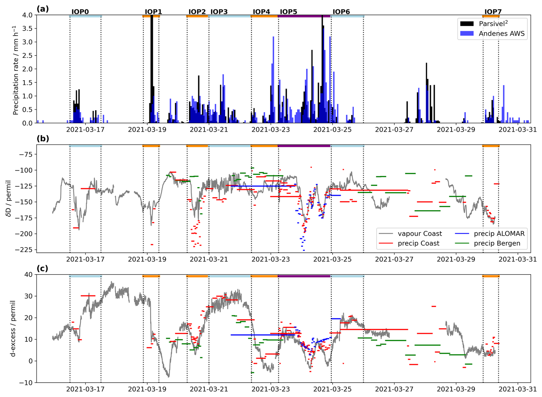
Figure 8 Time series of precipitation amount and precipitation isotope measurements at site Coast during ISLAS2021. (a) Precipitation rate (mm h⁻¹) from Parsivel² disdrometer (black) and Andenes AWS (blue). (b) Equilibrium vapour of precipitation, δD_p,eq, for precipitation sampled at sites Coast (red bars), ALOMAR (blue bars), and Bergen (green bars). Grey line shows water vapour δD measured at site Coast. (c) d-excess (‰) in precipitation samples (bars) at site Coast (red bars), ALOMAR (blue bars), and Bergen (green bars), and water vapour at site Coast (grey line). No offset has been applied to the precipitation d-excess scale. Light blue, orange and purple bars at the top of panels (a)–(c) denote IOPs.

During several IOPs, precipitation was collected at up to 10 min intervals for water isotope analysis (Sect. 2.2.4). It should be noted that the uncertainties in precipitation amount measurements do not transfer uncertainty towards the water isotope information in the precipitation samples unless one is interested in the amount-weighted isotope signal, for example in hydrological applications. In order to facilitate comparison with the vapour isotope measurements, we calculated the water vapour in isotopic equilibrium with the precipitation for the average air temperature of the precipitation interval at the respective sites. This so-called equilibrium vapour is denoted by δD_p,eq, and obtained from computing the vapour in equilibrium with the precipitation at a given temperature using established isotopic fractionation factors (Graf et al., 2019).

The high-resolution sampling revealed large short-term variations in the isotopic composition. During IOP0, the δD_p,eq varied between −160 ‰ and −30 ‰ (Fig. 8b, red bars). Distinct variations, albeit at lower magnitudes, were also observed during IOP1, IOP2, IOP5 and IOP7. The smaller variation in the precipitation suggests that the surface vapour follows the precipitation d-excess as a result of (often limited) below-cloud exchange processes (Graf et al., 2019). The vapour isotope composition measured at site Coast δD showed variations corresponding to the SWI in precipitation, albeit at a smaller amplitude (Fig. 8b, grey line). During IOP3 to IOP5, precipitation was also collected at ALOMAR at high resolution. Here, the δD_p,eq shows variations similar to those observed at Coast (Fig. 8b, blue bars). From 19 to 29 March 2021, precipitation was also collected at Bergen at high time resolution, with largest rainfalls during IOP2 to IOP4 (Fig. 8b, green bars). A comparison between the precipitation d-excess (not the equilibrium d-excess) with the water vapour d-excess at site Coast shows an astonishing degree of correspondence for several IOPs (Fig. 8c, red bars and grey line). For example, the transitions from IOP2 to IOP3, as well as from IOP4 to IOP5 match closely in terms of timing and magnitude. We consider this as support for the bias correction performed on the water vapour δ¹⁸O. The d-excess in precipitation from ALOMAR and Bergen is within 10 ‰ or less from the d-excess at site Coast.

5.3 Aerosol and INP measurements

During the campaign period, the INP concentration at site Coast varied between $\mathrm{6.7}\times {\mathrm{10}}^{-\mathrm{4}}$ and $\mathrm{3}\times {\mathrm{10}}^{-\mathrm{2}}$ (std L)⁻¹ at −15 °C and $\mathrm{5.8}\times {\mathrm{10}}^{-\mathrm{3}}$ and $\mathrm{1.5}\times {\mathrm{10}}^{-\mathrm{1}}$ (std L)⁻¹ at −20 °C (Fig. 9a). The highest INP concentrations were observed during the intense cyclone (IOP5) coinciding with the highest wind speeds and heaviest precipitation rates. Although, it should be noted that no clear relationship between INP concentration and wind speed was observed (Gjelsvik, 2022). Meanwhile, the lowest INP concentrations were observed during 27–28 March 2021, which was a period characterised by above-freezing temperatures, wind speeds between 5 and 10 m s⁻¹ and intermittent precipitation.

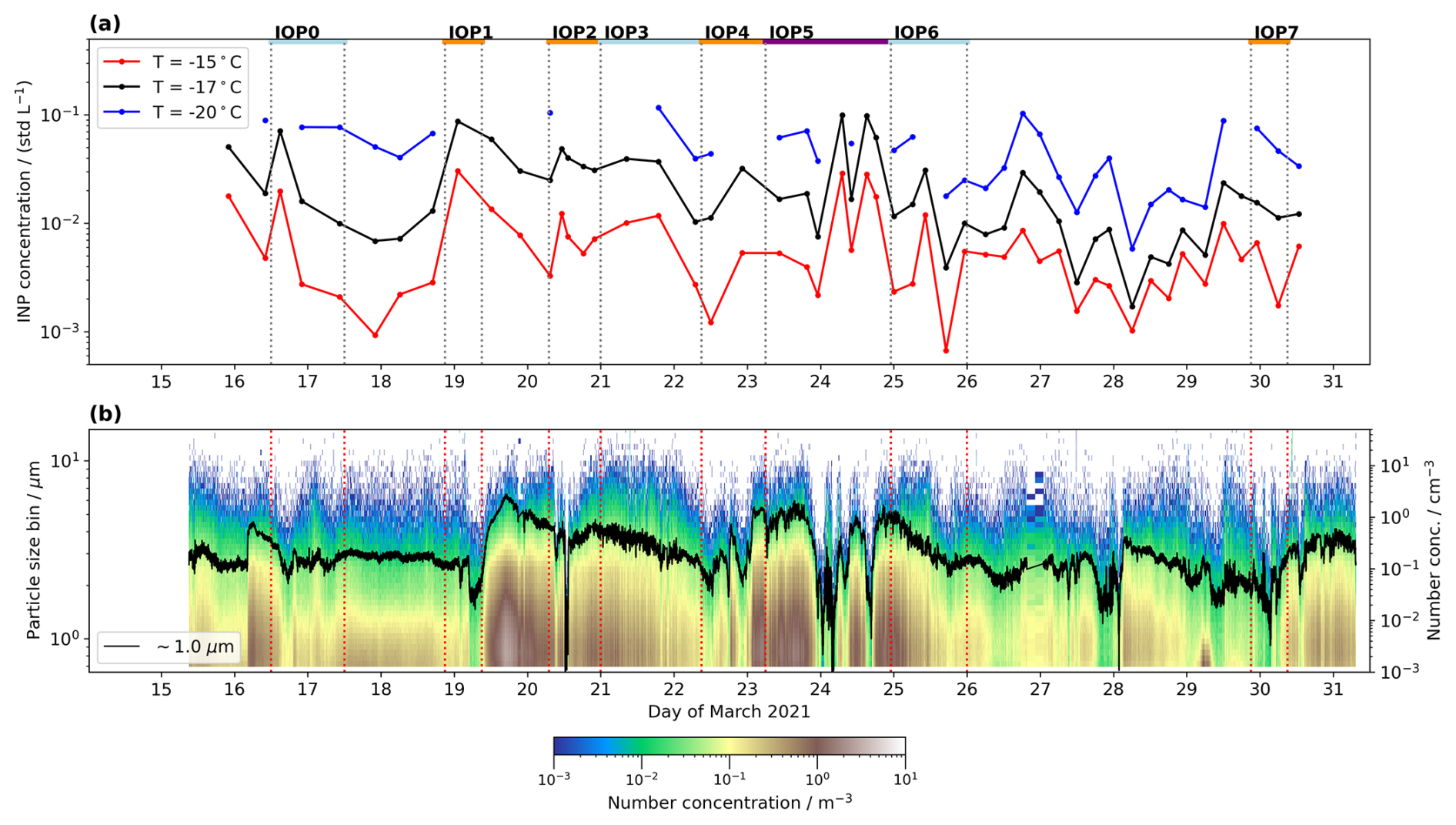
Figure 9 Observations of aerosols and ice nucleating particles (INP) at site Coast during ISLAS2021. (a) INP concentration in air collected at site Coast for freezing temperatures of $T=-\mathrm{15}$ °C (red), $T=-\mathrm{17}$ °C (black), $T=-\mathrm{20}$ °C (blue dots). Missing values at −20 °C are due to all of the wells freezing above this temperature, making it impossible to determine an INP concentration. (b) Time series of aerosols at site Coast from OPC and APS. The heat map shows particle number concentration (cm⁻³, shading; 1 µm, black line) as a function of time in logarithmic scaling. Vertical lines delineate IOPs indicated at the top of panel (a).

More generally, the INP concentrations observed during ISLAS2021 are similar to previous studies in the Norwegian Arctic. As shown by Gjelsvik et al. (2025), similar INP concentrations were observed during cold-air outbreaks on Andøya (Geerts et al., 2022) and during the fall and spring in Ny-Ålesund (e.g., Li et al., 2022). Even though these sites lie on opposite ends of CAOs and WAIs, the concentrations of INPs are comparable. Similarly to Lowenthal et al. (2016), who connected the isotopic fractionation of water vapour and precipitation to cloud microphysical processes, the observations presented here could in future work be exploited by linking the collocated INP and water isotope measurements to study differences in the ice-nucleating ability of different moisture and aerosol sources.

When comparing the INP concentration with the aerosol size distribution as measured by the APS, there is no clear relationship between periods of elevated INP concentrations and generally larger aerosol particles (Fig. 9b). This is consistent with the lack of relationship observed between the INP concentration and the aerosol concentration larger than 0.5 µm as measured by the OPC (Gjelsvik et al., 2025). The concentration of aerosol particles larger than 0.7 µm varied between 0.008 and 36.7 cm⁻³ with the highest concentrations occurring during high wind speeds in the afternoon of 19 March 2021 and the lowest concentrations occurring on the morning of 24 March 2021 during IOP5 (Fig. 9b). More generally, relatively clean periods were observed in conjunction with precipitation as expected due to wet-scavenging (e.g., Williams et al., 2024).

5.4 Horizontal precipitation transects

During the campaign period, a total of 8 horizontal transects of precipitation samples have been collected. These transect samples enable dataset users to assess the horizontal representativeness of the precipitation isotope measurements at sites Coast and ALOMAR within a range of up to 100 km. Due to their distance from the site Coast, the samples in the boxes were exposed to the atmosphere for up to several days before being collected. On some occasions, the box samples were also supplemented by surface snow samples collected nearby or at additional locations (Fig. 5). Since the sampling locations are roughly oriented in N–S orientation (Fig. 1b), the transect results are displayed using the latitude of the sampling locations as horizontal axis (Fig. 10).

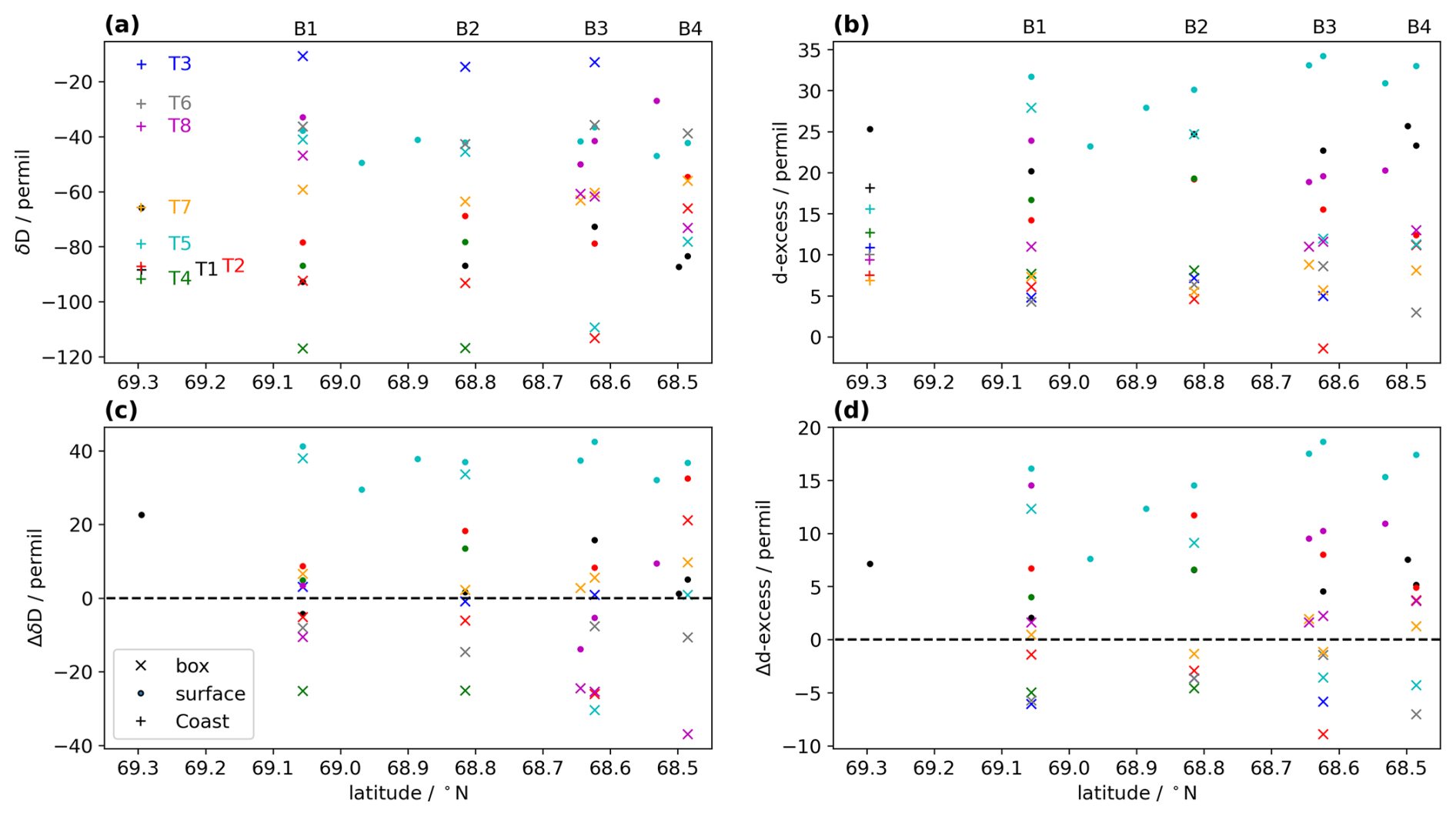
Figure 10 Horizontal precipitation isotope gradients from 8 sampling transects from Andenes towards the continent during ISLAS2021. (a) Precipitation δD (‰) in sampling boxes (x) and from surface samples (dots) compared to the average of corresponding precipitation at site Coast (+) vs. latitude of the sampling location (see Fig. 1b). Transects T1 to T8 are denoted by different colours. (b) As panel (a), but for precipitation d-excess (‰). (c) Difference between precipitation δD at all sampling locations an the corresponding precipitation at site Coast (ΔδD, ‰). (d) As panel (c), but for the difference in precipitation d-excess (Δd-excess, ‰).

The precipitation δD from boxes varies substantially between events, much more than between collection sites for the same event (Fig. 10a, coloured x). The average precipitation isotopes measured at site Coast for the corresponding period roughly agrees with the transect samples for most transects (coloured +). However, marked differences are noted for transect T3 and T4. These two transects were collected back-to-back during subsequent IOPs, and may contain spillover from the previous events due to delays in collecting the boxes. The correspondence to site coast is further highlighted by a difference plot (Fig. 10c), which confirms that all transects but T3 and T4 are within about 25 ‰ from the observations at site Coast. Thereby, events T8 and T6 show a slight tendency towards more depleted values, whereas T7 is less depleted.

The d-excess from the sampling boxes shows a more narrow distribution than δD with values between 5 ‰–10 ‰, and with more scatter at the more distant boxes (Fig. 10b, coloured x). This range of values is generally consistent with the average d-excess from corresponding precipitation at site Coast (coloured +). The difference plot in d-excess shows that the box samples are about 0 ‰ to 10 ‰ lower in d-excess, possibly indicating evaporation due to longer exposure times (Fig. 10d). However, the d-excess is substantially higher in all surface snow samples, compared to the corresponding box samples (Fig. 10b and d, coloured dots). The cause of this positive bias of about 20 ‰ or more in the surface snow samples is currently unclear, and may be related to mixing and exchange processes with the snow pack. Thus, while these transect samples deserve to be investigated more on a case-by-case basis, the fact that inter-event variations of up to 80 ‰ in δD are substantially larger than for the samples from a given transect (2 ‰–20 ‰) clearly indicates the possibility to determine the representativeness of Coast precipitation isotope measurements for the 100 km long transect across the Vesterålen archipelago.

5.5 Vertical water vapour isotope gradients at Andenes

The water vapour isotope measurements at sites Coast and ALOMAR were made at a horizontal distance of ∼2 km, and at an elevation difference of 364 m (Fig. 2a). Given sufficient accuracy and precision of the measurements, this setup enables the quantification of vertical gradients in the lower atmosphere during the campaign. As there is a temporal offset between the air masses arriving at the Coast and ALOMAR of several minutes (see below), we use 10 min averages to assess if a measurable gradient is present between the two locations. For δD, the probability density function leans to the left, showing a predominance of a negative gradient (Fig. 11a). The maximum is at −2 ‰, resulting in a gradient of $\sim -\mathrm{0.57}$ ‰ (100 m)⁻¹. In the large majority of cases, the difference is within ±5 ‰. For the d-excess, the gradient between ALOMAR and Coast $\mathrm{\Delta }d=d_{\mathrm{ALOMAR}}-d_{\mathrm{Coast}}$ (‰) is more pronounced, and predominantly negative (Fig. 11b). The maximum of the probability density function is at −5.2 ‰ corresponding to a d-excess gradient of 1.4 ‰ (100 m)⁻¹, with a secondary maximum close to zero. Due to both the offset applied to the δ¹⁸O data, and relatively low measurement precision of the analyser at site Coast, the vertical gradients of the d-excess are associated with larger uncertainty. Nonetheless, a gradient clearly emerges from the measurement uncertainty. Classification of the 10 min periods into IOP categories (Fig. 11, shading) shows that the strongest negative gradients are associated with mCAO periods when surface fluxes and non-equilibrium fractionation are strongest (Duscha et al., 2022; Sodemann et al., 2024). In comparison, the gradients are substantially smaller for most of the time during cases dominated by mid-latitude air advection. It will thus be possible to further utilise this dataset for finding how weather events are associated with more or less mixing, and stronger or weaker surface evaporation. We note that the gradients found here are quantitatively very similar when averaging the data at a 30 min time interval, confirming the robustness of the found gradient characteristics (not shown).

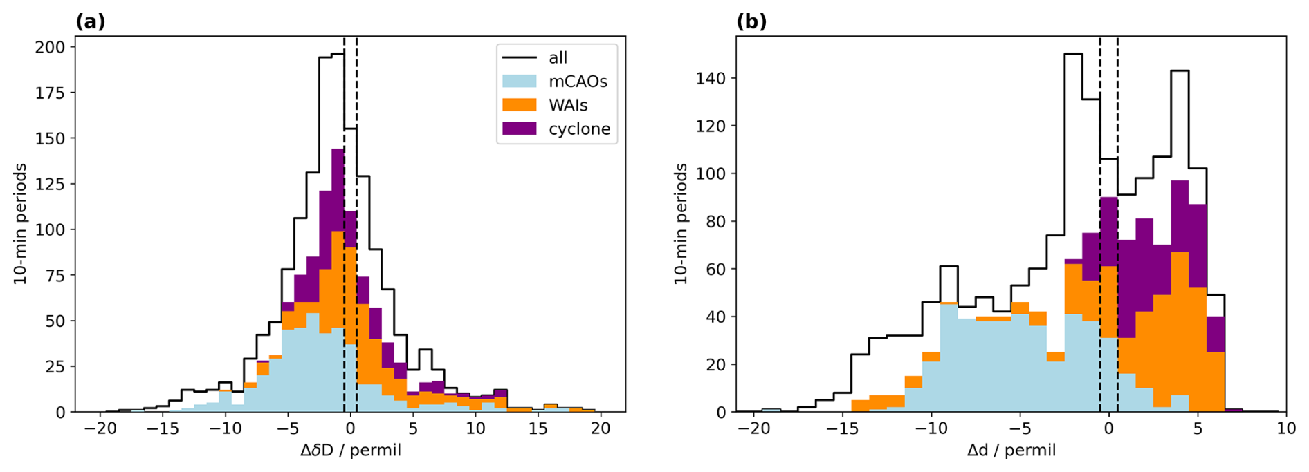
Figure 11 Vertical gradients in water vapour isotope measurements between sites ALOMAR and Coast of 10 min averaged measurement data. (a) $\mathrm{\Delta }\mathit{\delta }\mathrm{D}=\mathit{\delta }{\mathrm{D}}_{\mathrm{ALOMAR}}-\mathit{\delta }{\mathrm{D}}_{\mathrm{Coast}}$ (‰). (b) $\mathrm{\Delta }d=d_{\mathrm{ALOMAR}}-d_{\mathrm{Coast}}$ (‰). Black dashed lines denote the edges of bin zero. Histograms are further classified into mCAOs (light blue), WAIs (orange), and the intense cyclone during IOP5 (purple).

6 Combined case study for IOP2

We now illustrate how the combination of different measurement parameters from the ISLAS2021 campaign can provide complementary information. During IOP2 (07:00 UTC on 20 March to 00:00 UTC on 21 March 2021), a rapidly passing frontal wave dominated the weather evolution at Andøya. The front was immediately followed by a mCAO, that intensified strongly over the next day (IOP3, Fig. 4c). This air mass shift caused pronounced changes in several of the measured parameters. The time series of SLP at Andenes shows that the surface front passed at 14:30 UTC with a minimum pressure of 984 hPa (Fig. 12a, green line). Air temperature at site Coast was close to 2 °C before 09:00 UTC, when it stepped down to about 0.5 °C, followed by another downward step in air temperature at about 12:30 UTC (Fig. 12b). ALOMAR was below 0 °C throughout IOP2, except for a short uptick at 12:00 UTC, when the stratification was isothermal between both sites. Relative humidity (RH) at sites Coast, Slope and ALOMAR increased towards saturation around 09:00 UTC on 20 March 2021 (Fig. 12a), reflecting precipitation onset (Fig. 12e). While ALOMAR remained in saturated conditions for the remainder of IOP2, site Coast experienced again less saturated air masses after 18:00 UTC.

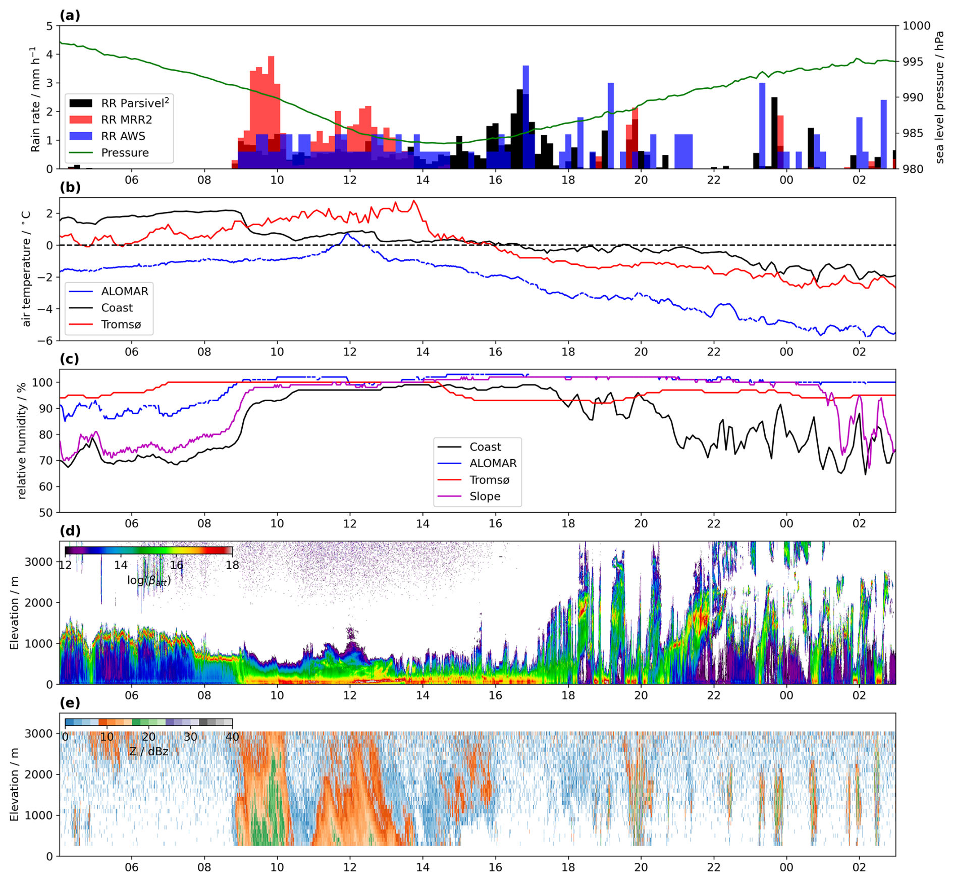
Figure 12 Meteorological measurements for IOP2 (00:00 UTC on 20 March 2021 to 06:00 UTC on 21 March 2021). (a) 10 min average rain rate (mm h⁻¹) from the Parsivel² disdrometer (black), from MRR2 at site Coast at 300 m above ground (red), and precipitation (blue) and sea-level pressure (green line) from the AWS at Andenes; (b) air temperature (°C) at site Coast (black line) and ALOMAR (blue line); (c) relative humidity (%) at sites Coast (black line), Slope (purple line), and ALOMAR (blue line); (d) range-corrected attenuated backscatter (shading, sr⁻¹) from the ceilometer CHM15 at Andenes, (e) radar reflectivity (shading, dBZ) from the MRR2 at site Coast.

The vertical structure of clouds and precipitation obtained from the MRR and the ceilometer corresponds to the changes in RH observed at the three sites. At 07:30 UTC on 20 March 2021, the cloud base dropped from 1000 to ∼700 m (Fig. 12d). Precipitation then set in at around 09:00 UTC according to the MRR reaching over the lowermost 1500–3000 m of the atmosphere (Fig. 12e). Precipitation rates at 300 m above ground were about 2–4 mm h⁻¹ according to the MRR (Fig. 12a, red), while the Parsivel² precipitation rate at ground level was below 2 mm h⁻¹ (black). Interestingly, the MRR did not record precipitation after 15:00 UTC, whereas the Parsivel² and the nearby Andenes AWS (blue) show the highest precipitation rates during that period. The ceilometer backscatter confirms continuing precipitation during that period, albeit with a more intermittent character after about 13:30 UTC. Visual observations of precipitation type report that melting snow dominated precipitation until about 13:00 UTC, which turned to rimed snowflakes thereafter. This suggests that in addition to limitations in detecting snow by the MRR, the receiver disk may have been covered by a snow layer, attenuating the reflected RADAR signal during this period. Reflectivity from the MRR at ALOMAR supports this interpretation (not shown).

The drop size distribution (DSD) during the main precipitation period of IOP2 between 09:00 to 18:00 UTC showed interesting variability (Fig. 13a). While the DSD showed a dominance of particles with size below 1 mm until about 13:00 UTC, the size distribution maxima increased to above 1 mm, and after 15:00 UTC showed an overall pronounced increase in particle number for up to 3 mm diameter as rain turned into snow. Similar size distributions also prevailed then for the more intermittent, convective precipitation after 18:00 UTC until the end of IOP2, still reaching the ground as snow. Changes in the DSD also correspond to changes in the aerosol load (Fig. 13b). With the onset of precipitation at 09:00 UTC, the aerosol number concentration decreases progressively at different size ranges, up to two orders of magnitude for the largest particles (3 µm, thick line). An uptick in aerosol load around 10:00 UTC corresponds to a change in the DSD. Between 12:30 to 14:00 UTC, a dramatic drop in the aerosol number concentration across all size ranges occurred, synchronous with the change to larger drop sizes, changes in wind direction and wind speed, vapour isotopes, and a drop in air temperature at site Coast (Fig. 12b).

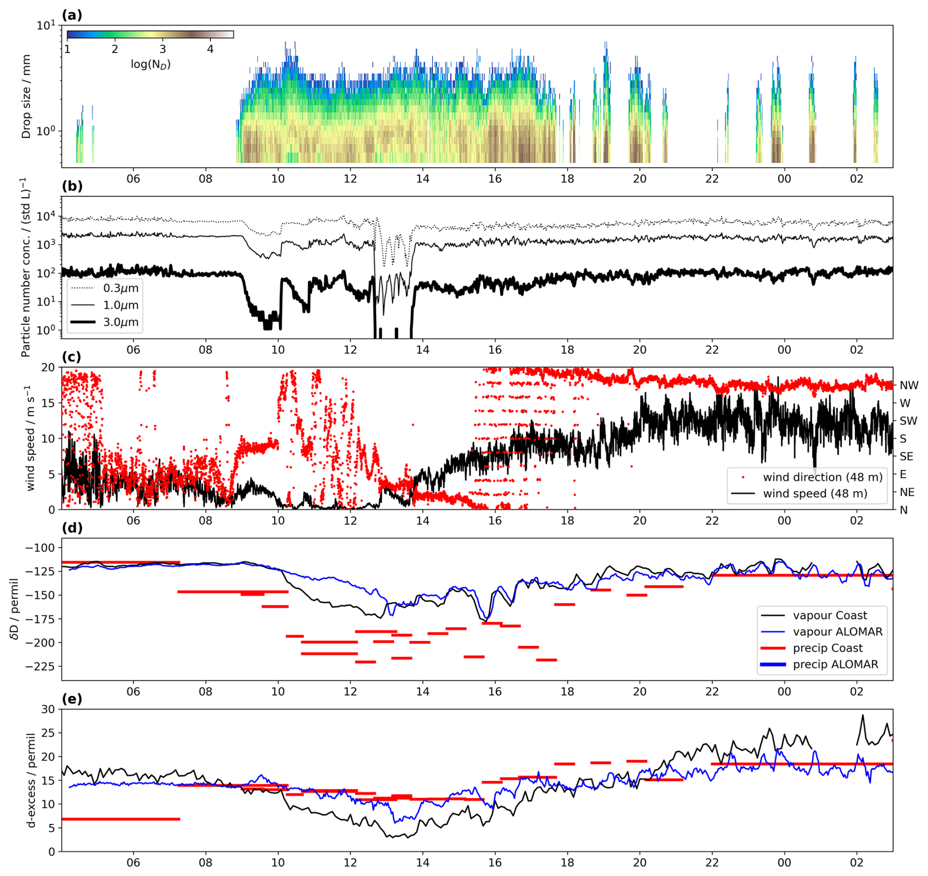
Figure 13 Precipitation, aerosol and water isotope measurements at Andenes for a time period containing IOP2 (20 to 21 March 2021). (a) Drop size distribution on a logarithmic scale from the Parsivel² disdrometer (shading); (b) particle number concentration ((std L)⁻¹) in logarithmic scaling for the size classes 0.3–0.5 µm (dotted line), 1.0–2.0 µm (solid line), and >3.0 µm (thick solid line) as measured by the OPC; (c) horizontal wind speed (m s⁻¹, black line) and wind direction (red dots) at 48 m measured at the meteorological tower at Oksebåsen, (d) water vapour δD (‰) at site Coast (black line) and ALOMAR (blue line), and equilibrium vapour in precipitation samples, δD_p,eq at site Coast (red bars); (e) water vapour d-excess at site Coast (black line) and ALOMAR (blue line), and precipitation d-excess at site Coast (red bars).

Finally, we describe the precipitation and vapour isotopes during this period. The maximum in air temperature, minimum in aerosol load, and change in drop size distribution coincides with the minimum in vapour d-excess (Fig. 13d), marking the end of a decline in water vapour δD after 09:00 UTC (Fig. 13c). Equilibrium vapour from precipitation samples, δD_p,eq, collected at high resolution during the event mirror the overall drop in water vapour δD, albeit with more pronounced variability. During the most intense precipitation period, δD_p,eq is more negative than vapour, denoting more depleted cloud signatures entering the boundary layer. ALOMAR vapour isotopes are becoming progressively less negative than at site Coast between 10:00 to 12:30 UTC, which could reflect the exchange between melting snow and water vapour at the lower elevation site Coast. Coherent oscillations in water vapour δD at both sites from 15:00 UTC until the end of IOP2 coincide with precipitation showers (Fig. 12a), and likely reflect vertical advection due to updrafts and downdrafts connected to convective cells in the CAO air masses passing over the site after the front (Fig. 12e). Similar co-variations between δD in precipitation and vapour are also observed at other IOPs (Fig. 8, IOP1 and IOP5).

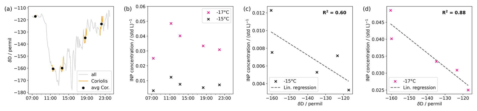
Figure 14 Synthesis of water isotope and INP measurements at Andenes for a time period within IOP2 (20 to 21 March 2021). (a) Water vapour δD (‰) at site Coast (all data, grey line), during coincident INP measurements (Coriolis, orange line), and average over 40 min of coincident INP measurements (avg Cor., black circle). (b) INP concentration (std L⁻¹) at −15 °C (black crosses) and −17 °C (pink crosses). (c) Dependence of INP concentration at −15 °C on δD (black crosses) and linear regression line (black dashed line). (d) Dependence of INP concentration at −17 °C on δD (pink crosses) and linear regression line (black dashed line).

During IOP2, five aerosol INP measurements were conducted that coincided with the SWI measurements. While the water vapour δD rapidly decreased from −120 ‰ to −175 ‰ in the beginning of IOP2 before increasing again to −115 ‰ at the end of IOP2 (Fig. 14a), the measured INP concentrations at −15 and −17 °C show the opposite behaviour (Fig. 14b). Indeed, we find an anti-correlation between the INP concentrations and δD measured in air throughout IOP2 (Figs. 14c and d, with R² values of 0.6 at −15 °C and 0.88 at −17 °C, respectively). The general expectation is that precipitation removes the most active INPs from the airmass during transport. As the amount of precipitation removed from the airmass (more negative δD) does not reduce the INP concentrations, this suggests a local source of INPs throughout the warm air intrusion of IOP2. However, further analysis is needed to investigate the influence of other explanations, such as shifts in air mass origin or the modification during transport for the observed anti-correlation. Nevertheless, these findings exemplify the added value of combined SWI and aerosol INP measurements pertaining to, for example, INP source attribution.

A brief inspection of all IOPs reveals that co-variations in the aerosol size distribution and δD are common, albeit on different time scales, and non-uniformly for the different IOPs (not shown). Unraveling the reasons behind such intermittent co-variations clearly motivate further investigation of the interrelation of aerosols and water isotopes in Arctic weather systems based on the ISLAS2021 dataset.

7 Discussion of spatial representativeness

We assess the spatial representativeness from the ability of the network to detect co-variations in the vapour isotope signals with or without time offsets, while taking into account the combined measurement uncertainty of the CRDS analysers. The ambient variation of isotope composition reaches often values of 20 ‰ for δD and 2.5 ‰ for δ¹⁸O within 30 min, more than an order of magnitude larger than the respective typical combined uncertainties of 1 ‰ and 0.15 ‰ (Figs. 6 and 13c). The collocated installation of two CRDS at different elevations provides confirmation that these variations are due to meteorological phenomena, and that they are not fundamentally compromised by the larger uncertainty of the CRDS at site Coast. The detection of local-scale differences for the d-excess, however, is only possible in situations where the uncertainty is less than the signal, for example during situations of stable stratification (Fig. 11). By detecting both time offsets, but also modifications of signals in δD and δ¹⁸O over distance, the measurement network allows one to detect how atmospheric processes such as rain evaporation, mixing, and also horizontal variations of air masses have modified the atmospheric water vapour isotope composition over the time it takes an airmass to pass the 100 km distance (typically 2–6 h). Examples for periods where such horizontal representativeness is evident are the large W-shape variations of isotope composition during IOP5, which is apparent near-simultaneously at Coast and ALOMAR, and with a delay of 2 h also at Tromsø (Fig. 6, 24 March 2021). The network thus captures consistent isotope signatures that are associated with meso to synoptic-scale phenomena at this 100 km scale.

The measurement station in Bergen (1100 km distance) is generally more disconnected from the weather evolution in the northern locations, but captures for example similar signatures as the northern network during the mCAO period of IOP3 (Fig. 6). Interestingly, co-variations in the d-excess are sometimes more obvious across the entire network than for δD and δ¹⁸O, such as during IOP5 (Fig. 6d). A more detailed analysis using trajectory calculations or similar transport modelling tools are needed to better understand why such larger-scale co-variations are sometimes present, and sometimes not.

8 Data availability

The ISLAS2021 datasets described and presented here are available as a dataset bundle for the individual instruments at https://doi.org/10.1594/PANGAEA.984616 (Sodemann et al., 2025). Measurements of the aerosol INP concentrations and the OPC are described in Gjelsvik et al. (2025) and published on Zenodo (Gjelsvik et al., 2024, https://doi.org/10.5281/zenodo.11617774). The precipitation INP concentrations are included in the dataset bundle on PANGAEA (https://doi.org/10.1594/PANGAEA.984616, Sodemann et al., 2025). It is important to note that the precipitation samples may have been influenced by blowing and drifting snow and some samples required dilution for a complete analysis to take place. Therefore, we strongly encourage the data users to reach out to the data providers before using the precipitation INP data. In addition, several datasets have been included in the data presentation of this manuscript but are already described elsewhere. INP from sea water samples are available in Gjelsvik (2022) (https://doi.org/10.5281/zenodo.17085170). The meteorological data from the AWS in Andøya and Bergen (station numbers: SN87110 and SN50540, respectively) are available at the website: https://seklima.met.no/observations/ (last access: 8 April 2026). Sea-ice edge data are available at https://doi.org/10.24381/cds.29c46d83 (Copernicus Climate Change Service, 2020).

9 Conclusions

The ISLAS2021 field campaign aimed at collecting a combined dataset of water vapour and precipitation isotopes, supplemented by aerosol and INP measurements, across several sites of a mesoscale measurement network. Located at the west coast of Northern Norway, and taking place during winter time, the measurement sites experienced strongly varying weather conditions, dominated by either arctic or mid-latitude weather systems. From a general dataset perspective, the following aspects are particularly worth noting:

1. Water vapour isotope measurements have been performed simultaneously at four observatories at a horizontal distance from less than 1 km to up to 1000 km, and with an elevation difference of 364 m. With careful calibration and post-processing of each analyser, it is possible to reliably compare measurements across the network for the main isotopes, δD and δ¹⁸O. The d-excess parameter was associated with larger uncertainty for one analyser, but does generally allow for a direct comparison of signals of moisture origin arriving at different locations.

2. Comparisons between the sites that are 1000 km apart show generally large differences in specific humidity and water vapour isotopes, whereas clear co-variations with time shifts are seen at a scale of 100 km. This implies that vapour isotope measurements are representative on a scale of 100 km, while a comparison at 1000 km is only meaningful in flow configurations where the stations are upstream or downstream of one another. Such connections can for example be identified with the help of Lagrangian airmass transport calculations.

3. The set-up with two nearby water vapour analysers at an elevation difference of 364 m enables the assessment of vertical gradients in main isotopes and the d-excess. The median vertical gradients during the campaign period are $\sim -\mathrm{0.57}$ ‰ (100 m)⁻¹ for δD, and 1.4 ‰ (100 m)⁻¹ for the d-excess. These gradients vary with weather situation, and need to be interpreted with extra care for the d-excess and δ¹⁸O, as they are dependent on corrections needed for the analyser at the Coast location.

4. Isotopes of precipitation collected at very high time resolution during several Intense Observation Periods (IOPs) showed strong correspondence with the vapour signals. As the precipitation isotopes can be determined with a higher analytical precision, their correspondence with the water vapour isotope measurements provides independent confirmation of the main isotopes and the d-excess in ambient air.

5. Horizontally distributed precipitation and surface snow samples complement the high-resolution local sampling with a first-order estimate of the spatial representativeness of the stable isotope composition in precipitation from different weather systems. We find that event-scale precipitation isotope data collected across a 100 km long transect over the Vesterålen archipelago are characterised by much smaller isotope variability than inter-event variations.

6. Aerosols and INPs complement water isotope and precipitation sampling meaningfully, as both are related to microphysical processes within and below clouds. In particular, their synergy allows for INP source attribution (e.g. local vs. remote source regions) depending on how much distillation the SWIs indicate.

In summary, the ISLAS2021 dataset provides insight into the representativeness of water vapour isotopes in sub-arctic weather systems, that are characterised by intense turnover of water vapour at regional scales. The rare combination of stable water isotope measurements in water vapour and precipitation, and with aerosol composition can be valuable for a range of forthcoming studies. These include, for example, process studies and model validation of coastal mixed-phase clouds and precipitation in convective and stratiform cloud regimes, the understanding of INPs for sub-Arctic precipitation processes, improving Earth System Models for the present day Arctic climate (Gjelsvik et al., 2025), the assessment of the representativeness of stable water isotope measurements in water vapour and precipitation on a scale of up to 1000 km in different weather situations, the quantification of precipitation efficiency in high-latitude storms from stable water isotope measurements, and the analysis of the d-excess as a tracer of moisture source conditions. Such studies could be done with full-scale isotope-enabled atmospheric models and in more idealised, process-based frameworks. The ISLAS2021 dataset can therefore contribute both to improved understanding of how atmospheric processes shape the stable isotope signal in water vapour and precipitation, and to improved representation of sub-grid scale processes associated with clouds and precipitation in numerical weather prediction models.

Appendix A: Installation site details

The water vapour isotope measurements during ISLAS2021 in Northern Norway were set up at three different locations. As the location of the inlet lines for ambient air are important to assess the representativeness of the measurements, as well as potential error sources, they are documented visually in this Appendix. The inlet system at site Bergen has been documented in Weng et al. (2021).

Water vapour isotope measurements at site Coast were set up in a wooden building close to the coast (Fig. A1a). The building was situated in the immediate vicinity of the coast (Fig. A1b), and next to a steep rock face of Anhauet mountain (Fig. A1a). The heated inlet line was installed on the NE corner of the building with free fetch from the ocean in northerly directions (Fig. A1b). The location and instrumentation of site Coast are further described in Sect. 2.2.

Water vapour isotope measurements at site ALOMAR were set up in a small housing that is normally used to operate the main hatch of the observatory (Fig. A2c). The heated ambient air inlet was installed facing W on a ladder at rooftop level (Fig. A2a). The precipitation totalisator for liquid measurements and a collection box were installed immediately N of the air inlet at the railing of the platform (Fig. A2b). The location and instrumentation of site ALOMAR are further described in Sect. 2.3.

Water vapour isotope measurements at site Tromsø were installed at the University campus near the city centre of Tromsø (Fig. A3a, marker). The campus is located on the NE edge of the island of Tromsø (Tromsøya). The natural sciences building overlooks the surrounding buildings (Fig. A3b). The heated inlet was installed on a pole, pointing to the W over the railing. The location and instrumentation of site ALOMAR are further described in Sect. 2.6.

The snow sampling boxes along the horizontal transect were placed in the open landscape at ground level (Fig. A5). Small bushes, fences, or other structures were used to attach the boxes, keeping them in place for extended sampling periods. Sampling locations were typically surrounded by a layer of surface snow, that could have contributed to snow in the sampling boxes, in particular during strong wind events.

Table A1 Time periods of horizontal transect sampling from boxes and surface snow during ISLAS2021.

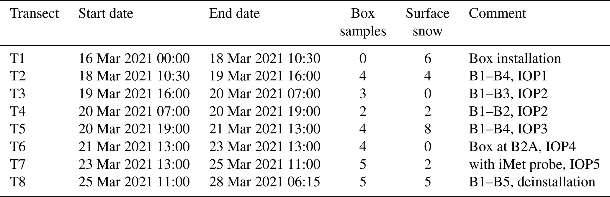
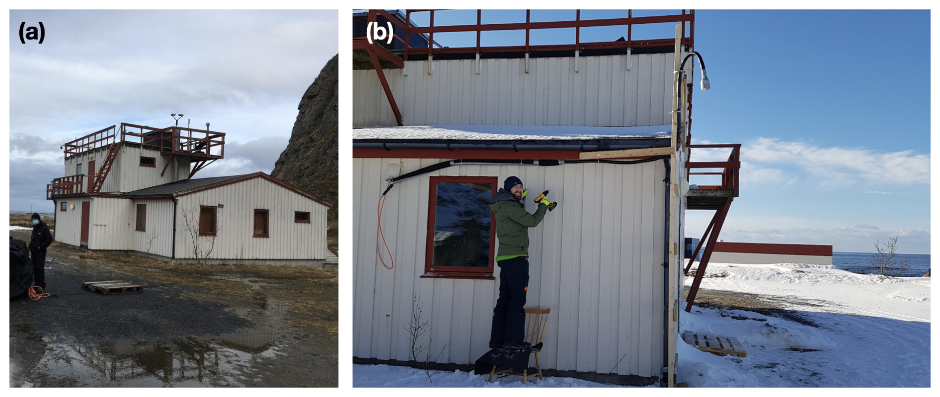
Figure A1 (a) Site Coast seen from SW direction with Adhauet mountain to the right. The Parsivel² disdrometer, Micro rain radar, and aerosol inlet are visible on the top of the building. (b) Heated inlet for water vapour isotope sampling at site Coast looking W towards the Norwegian Sea.

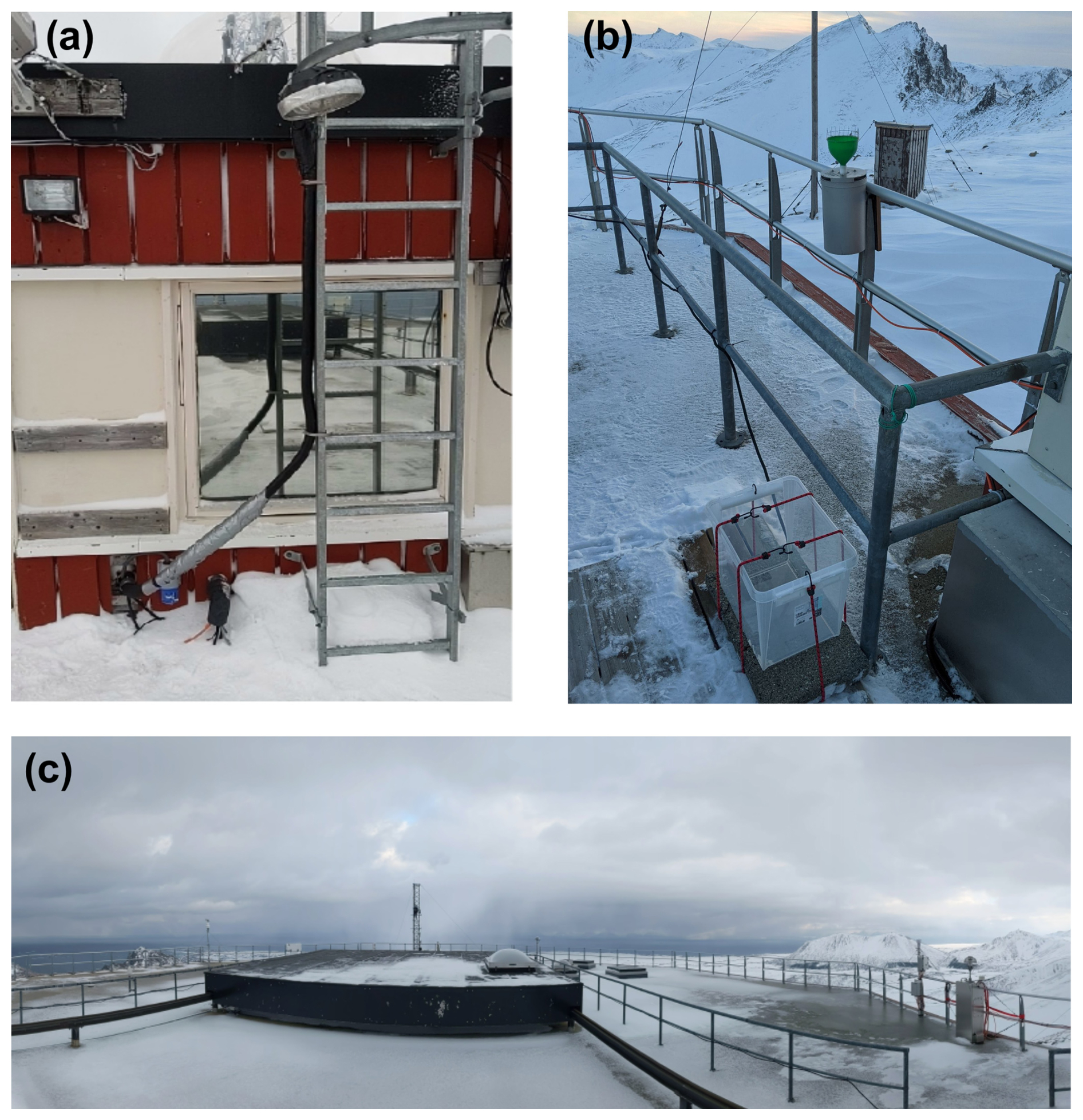
Figure A2 (a) Inlet for vapour measurements and (b) setup of sampling box and precipitation totalisator. (c) Rooftop of ALOMAR main building showing sliding doors for lidar measurements.

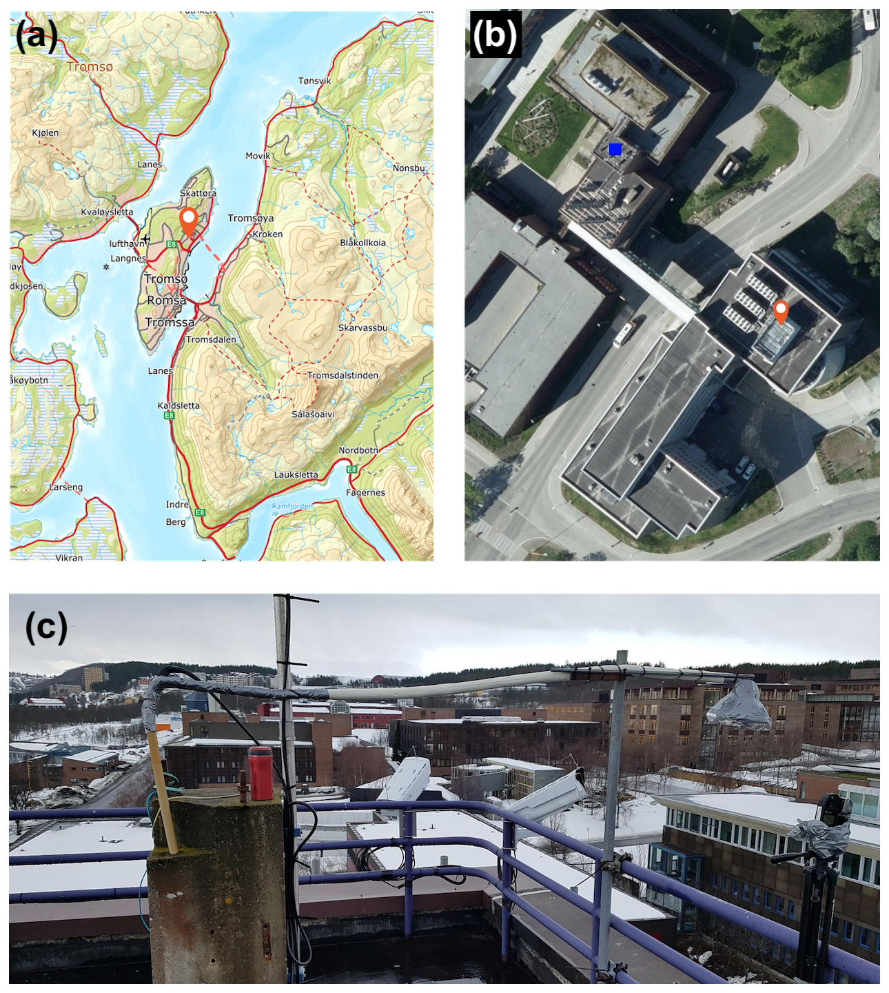
Figure A3 (a) Tromsøya with the location of UiT, and (b) the Natural Science building at the university campus, where the blue square denotes the position of the air inlet and AWS. (c) Ambient air inlet for water vapour isotope measurements on the roof of the University of Tromsø natural sciences building. The maps in (a) and (b) are from https://norgeskart.no/ (last access: 8 April 2026).

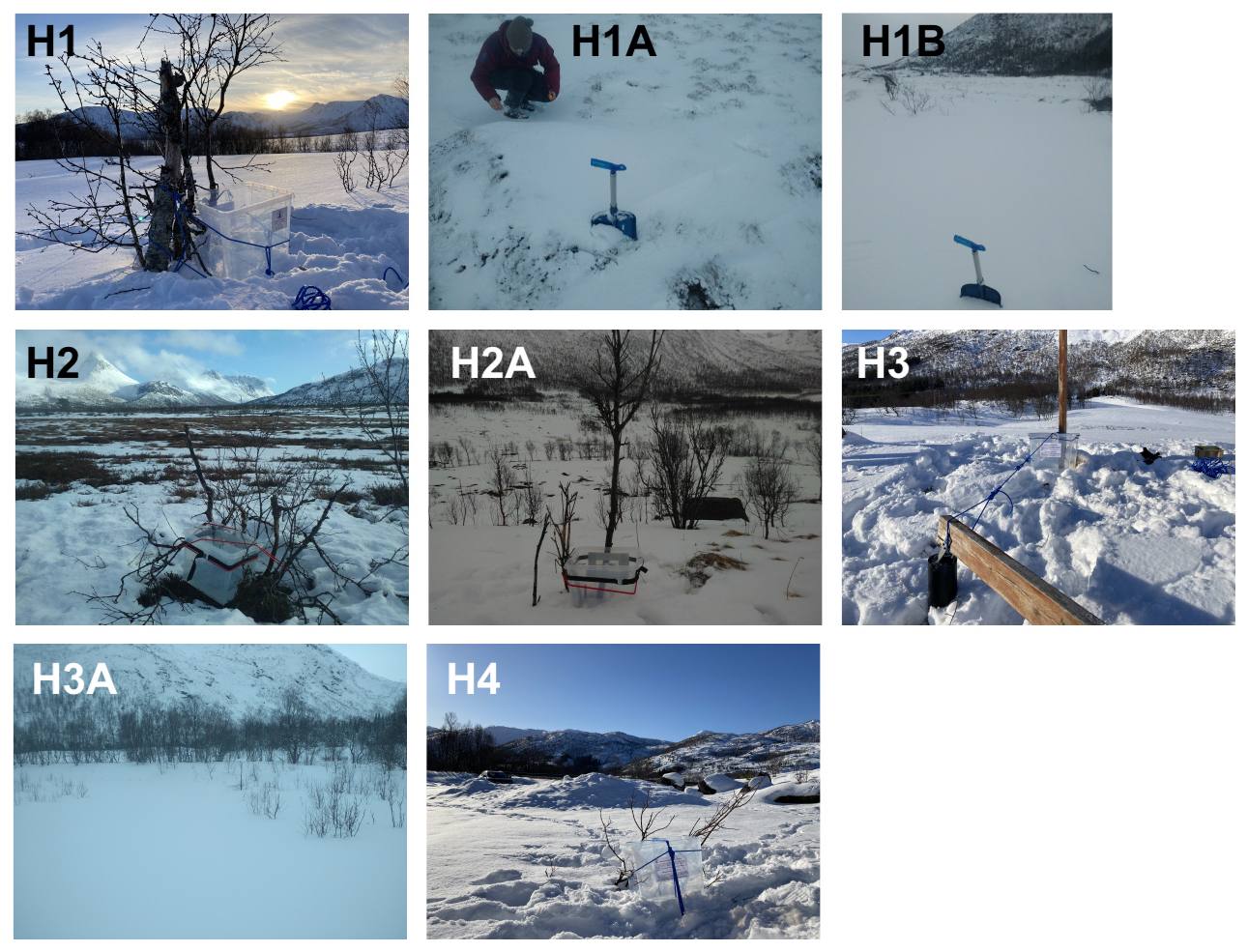
Figure A4 The boxes and surface snow sampling sites for locations H1–H4 along the horizontal transect.

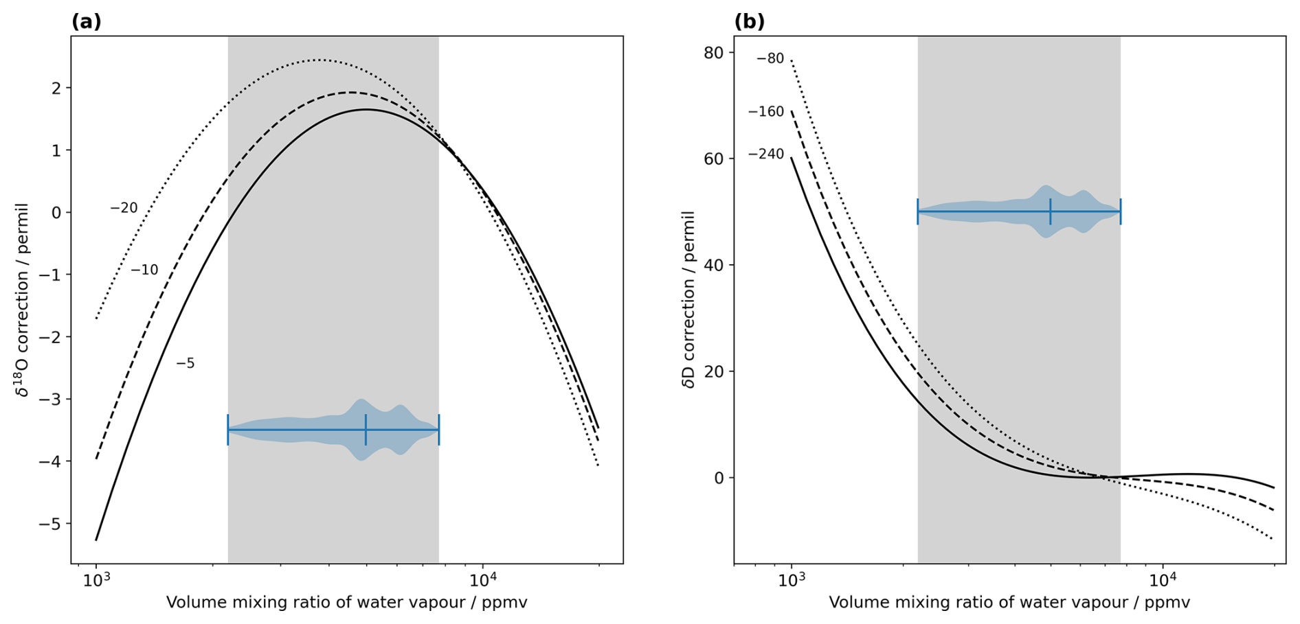
Figure A5 Isotope ratio–mixing ratio correction functions for Picarro analyser HIDS2380 determined immediately after the ISLAS2021 field deployment for (a) δ¹⁸O and δD. The isotope ratio–mixing ratio dependency is particularly strong below a mixing ratio of 1000 ppmv for this particular analyser. Different lines show the correction for different isotope ratios (‰). The grey shaded are denotes the range covered by measurements during ISLAS2021. The blue violin plot indicates data density for different mixing ratios. Note the log scale for the horizontal axis.

Appendix B: Long-term calibration coefficients

Water vapour isotope measurements were normalised to VSMOW-SLAP scale using long-term calibration coefficients (slope and offset, Table B1). These calibration coefficients are analyser dependent, and have been established from repeated measurements of several secondary standards, including controlled laboratory environments. For see Sect. 4.1 for context.

Table B1 Long-term calibration coefficients for the CRDS analysers for water vapour isotope measurements used during the ISLAS2021 field campaign.

Appendix C: Isotope ratio–mixing ratio dependency corrections

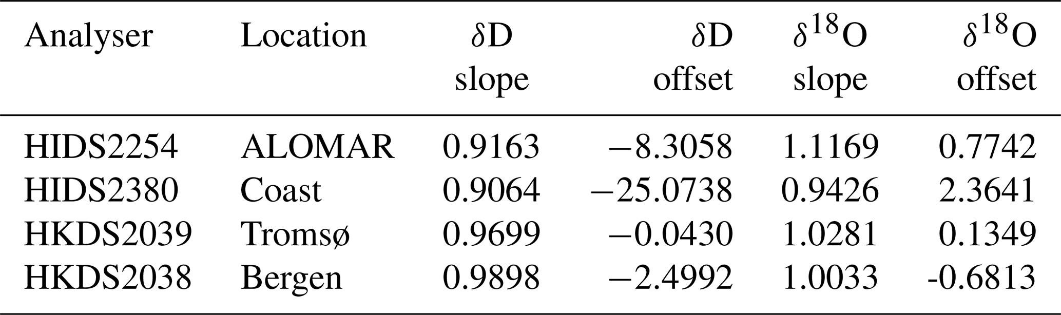
Water vapour isotope measurements of the Picarro L2130-i CRDS with serial number HIDS2380 were corrected using the method of Weng et al. (2021) and Sodemann et al. (2023b). This particular analyser has an unusually strong isotope ratio – mixing ratio dependency, which required correction of ±2 ‰ within the mixing ratios encountered here, and up to 50 ‰ for the δD at the lowest mixing ratios. The correction functions applied to the raw dataset are given below. Thereby, x is the natural logarithm of the water vapour mixing ratio, and y is the uncalibrated delta value of δ¹⁸O or δD as reported by the analyser.

The correction function polynomials z(x,y) with coefficients p₀₀ to p₁₂ for δ¹⁸O at a reference humidity 10 000 ppmv are:

$$\begin{array}{}\text{(C1)}& \begin{array}{rl}{z}^{\mathrm{18}}& =p_{\mathrm{00}}+p_{\mathrm{10}}x+p_{\mathrm{01}}y+p_{\mathrm{20}}{x}^{\mathrm{2}}+p_{\mathrm{11}}xy+p_{\mathrm{02}}{y}^{\mathrm{2}}\\ & +p_{\mathrm{30}}{x}^{\mathrm{3}}+p_{\mathrm{21}}{x}^{\mathrm{2}}y+p_{\mathrm{12}}x{y}^{\mathrm{2}}.\end{array}\end{array}$$

The respective coefficients for δ¹⁸O and for δD obtained from laboratory characterisation at FARLAB during 2021 are given in Table C1.

Table C1 Coefficients for correcting the isotope ratio-mixing ratio dependency for Picarro CRDS analyser at site Coast (Ser. No. HIDS2380), determined at FARLAB in 2021.

Appendix D: Calculation of the uncertainty budget for water vapour isotope measurements

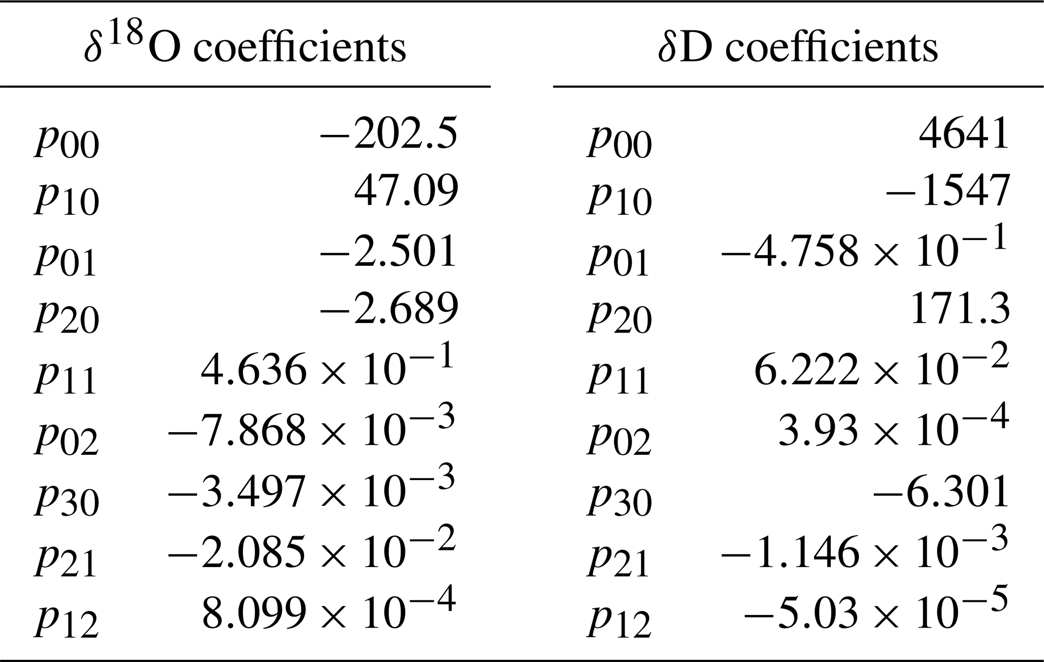
Calibration of the water vapour isotope measurements is done using procedures recommended by IAEA (2017):

$$\begin{array}{}\text{(D1)}& {\displaystyle }& {\displaystyle }\mathit{\delta }{\mathrm{D}}_{\mathrm{smp}}=\mathit{\delta }{\mathrm{D}}_{\mathrm{h}}+\left(\mathit{\delta }{\mathrm{D}}_{\mathrm{l}}-\mathit{\delta }{\mathrm{D}}_{\mathrm{h}}\right)\cdot f\text{(D2)}& {\displaystyle }& {\displaystyle }f=\left(\mathit{\delta }{\mathrm{D}}_{\mathrm{sample}}^w-\mathit{\delta }{\mathrm{D}}_{\mathrm{h}}^w\right)/\left(\mathit{\delta }{\mathrm{D}}_{\mathrm{l}}^w-\mathit{\delta }{\mathrm{D}}_{\mathrm{h}}^w\right).\end{array}$$

Hereby, δD_sample is the calibrated δ value of the sample, δD_h and δD_l denote the calibrated values of the isotopically heavy (h) and light (l) working standards, and w denotes the raw values of the standard and sample. Corresponding equations exist for the other isotope species. A set of secondary standards normalised to VSMOW-SLAP scale with assigned values listed in Table D1 was used for calibration of all four CRDS analysers in the measurement network.

The combined or total uncertainty of the calibrated samples is then estimated from an error budget, involving the following components (Gröning, 2011):

1. u_c(h): calibration uncertainty, assigned uncertainty of the isotopically heavy standard h

2. u_c(l): calibration uncertainty, assigned uncertainty of the isotopically light standard l

3. u_a(H): analytical uncertainty, uncertainty of measured values of isotopically heavy standard H, estimated from SEM of repeated standard measurements

4. u_a(L): analytical uncertainty, uncertainty of measured values of isotopically light standard L, estimated from SEM of repeated standard measurements

5. u_m: measurement uncertainty, estimated from the standard deviation within a given averaging interval of the measurement time series

Table D1 Stable water isotope composition of secondary standards used for calibration of CRDS water vapour isotope measurements during the ISLAS2021 field campaign (‰). Uncertainties (u, ‰) are obtained from long-term repeated measurements against primary standards (VSMOW, SLAP) provided by IAEA.

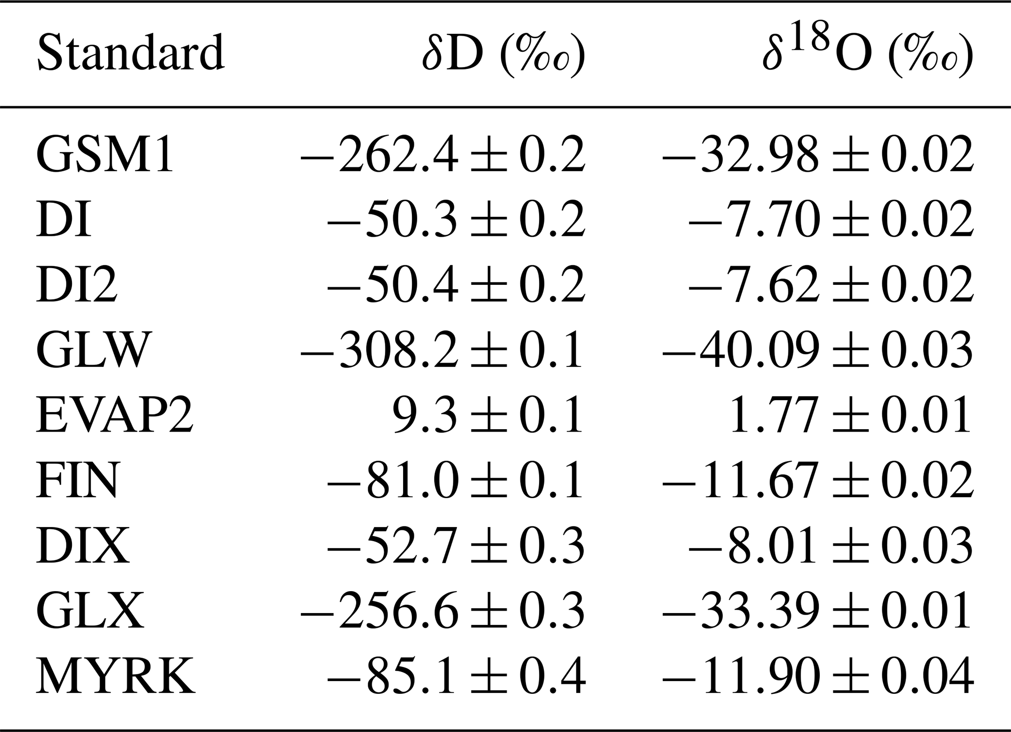
The combined (total) uncertainty u_t is then calculated from the square root of the squared sum of all error components of the budget, weighted by the respective sensitivities, using

$$\begin{array}{}\text{(D3)}& u_{\mathrm{t}}=\sqrt{s_{\mathrm{h}}^{\mathrm{2}}u(h{)}^{\mathrm{2}}+s_{\mathrm{l}}^{\mathrm{2}}u(l{)}^{\mathrm{2}}+s_{\mathrm{H}}^{\mathrm{2}}u(H{)}^{\mathrm{2}}+s_{\mathrm{L}}^{\mathrm{2}}u(L{)}^{\mathrm{2}}+s_{\mathrm{m}}^{\mathrm{2}}u(m{)}^{\mathrm{2}}}.\end{array}$$

Here, s_h, s_l, s_H, s_L and s_m are sensitivities of the form

$$\begin{array}{}\text{(D4)}& s_{\mathrm{h}}=\partial f/\partial {\mathit{\delta }}_{\mathrm{h}}\end{array}$$

according to each of the five elements of the error budget (Gröning, 2011), and f denotes the calibration function (Eq. D2).