the Creative Commons Attribution 4.0 License.
the Creative Commons Attribution 4.0 License.
 | 02 Apr 2026
A first approach towards dual-hemisphere sea ice reference measurements from multiple data sources repurposed for evaluation and product intercomparison of satellite altimetry
Henriette Skourup
Heidi Sallila
Stefan Hendricks
Renée Mie Fredensborg Hansen
Stefan Kern
Stephan Paul
Marion Bocquet
Sara Fleury
Dmitry Divine
Eero Rinne
Sea ice altimetry currently remains the primary method for estimating sea ice thickness from space, however, time series of such satellite-derived estimates are of limited use without having been quality-controlled against reference measurements. Such reference measurements (a term encapsulating in situ observations and remotely sensed measurements from ground, air, and below the ice) for validation of altimetry measurements over sea ice in the polar regions are sparse and rarely presented in a manner where the time-space averaging matches that of the satellite-derived products. Here, an approach to a published comprehensive collection of sea ice reference measurements repurposed for satellite altimetry observations over sea ice is presented, which includes estimates of freeboard, thickness, draft and snow depth from sea ice-covered regions in the Northern Hemisphere (NH) and the Southern Hemisphere (SH), all of which are relevant for comparison with altimetry estimates. The measurements have been collected using airborne sensors, autonomous drifting buoys, moored and submarine-mounted upward-looking sonars, and visual observations. The data package has been prepared to match the spatial (25 km for NH and 50 km for SH) and temporal (monthly) resolutions of conventional satellite altimetry-derived sea ice thickness data products for a direct evaluation of these, and the code is publicly available and distributed for users to modify depending on their aim. This data package, also known as the Climate Change Initiative (CCI) sea ice thickness (SIT) Round Robin Data Package (RRDP), was produced within the ESA CCI Sea Ice project. The current version of the CCI SIT RRDP covers the polar satellite altimetry era (1993–2024) and has ongoing efforts aimed at continuously updating the datasets. The CCI SIT RRDP has been collocated with satellite-derived sea ice thickness products from CryoSat-2, Envisat, and ERS-1/2 produced within the ESA CCI and the Fundamental Data Records for Altimetry (FDR4ALT) projects to demonstrate the overlap and inter-comparison between the reference measurements and satellite-derived products. Here, the CCI SIT RRDP is introduced along with examples of its use as a validation source for satellite altimetry products, where the averaging, collocation and uncertainty methodology is presented, and advantages and limitations are discussed. The CCI SIT RRDP dataset is available at https://doi.org/10.11583/DTU.24787341 (Olsen and Skourup, 2026a).
- Article
(7701 KB) - Full-text XML
- BibTeX
- EndNote


Comprehensive validation of satellite altimetry–derived sea ice thickness (SIT) Climate Data Records (CDRs) requires coincident observations of sea ice freeboard, thickness, snow depth, and densities of snow, ice and water (Fig. 1), following the assumption that sea ice is in hydrostatic equilibrium. Ideally, such measurements should match the spatial and temporal scales of the satellite data and cover the entire polar satellite altimetry era, beginning with the launch of the European Space Agency (ESA) ERS-1 mission in 1991 and its subsequent collection of scientific altimetry data over sea ice as of 1993. However, such observations are sparse and unevenly distributed across the Arctic and, even more so, in the Antarctic due to logistical constraints and high operational costs. In addition, most existing measurements provide only a subset of the required variables. Examples of these include: snow depth and total freeboard from coincident airborne snow radar and laser, draft from upward-looking sonar moorings, or snow depth and SIT from drifting buoys. Measurements of the densities of snow, sea ice, and water are even more limited than the above-mentioned parameters and are therefore not examined in this study.
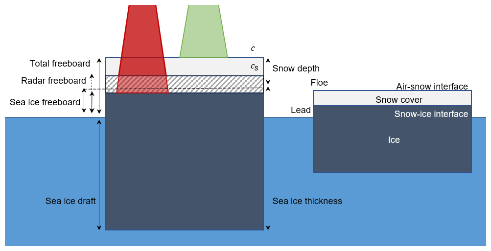
Figure 1Schematic of the different sea-ice-altimetry-related terms. Radar (Ku-band) and laser altimetry observations and their expected penetration into the snow pack are shown by the red and green beams, respectively. Not to scale. The shaded area denotes the uncertainty related to penetration of radar and slowdown of propagation speed, which depends on the snow conditions, and impacts (along with other things) the retrieved radar freeboard.
We use the term reference measurements for such a compilation of independent non-satellite observations collected from airborne platforms, submarines, moorings, drifting buoys, and ships, which can potentially be used for evaluation of satellite-derived SIT CDRs. These should not be confused with Fiducial Reference Measurements (FRMs), which follow strict protocols and standards that are still being defined for SIT validation (e.g., Da Silva et al., 2023). Here, we present and evaluate a collection of existing, publicly available, freeboard, thickness, draft, and snow depth reference measurements from various sources. These measurements were compiled within the ESA Climate Change Initiative (CCI) Sea Ice project (https://climate.esa.int/en/projects/sea-ice/, last access: 11 August 2025) as part of the Round Robin Data Package (RRDP), hereafter referred to as the CCI SIT RRDP.
The overarching aim of the ESA CCI Sea Ice project is to produce CDRs of SIT (and sea ice concentration) from existing polar radar altimetry (and passive microwave radiometry) missions dating back to 1993 (or 1972) without inter-satellite-mission biases. This requires careful treatment of differences in spatial coverage, footprint sizes, resolution, and instrument design between missions. The specific purpose of the CCI SIT RRDP is to provide a set of independent, non-satellite reference measurements covering the polar satellite altimetry era, prepared to a level comparable with the CCI SIT CDRs. However, we acknowledge that the datasets in the CCI SIT RRDP were not inherently collected or post-processed with the aim of satellite evaluation; thus, careful consideration of inherent biases, preferential sampling, and measurement uncertainties is critical.
In line with metrological principles, reference measurements themselves require validation – a requirement that is not always met. A key question is whether a given reference dataset is fit-for-purpose, i.e., adequate for SIT or snow depth validation without introducing selection biases (e.g., Langsdale et al., 2025). To address this, we performed a literature-based assessment of each dataset's validation efforts, noting limitations such as preferential sampling or known measurement biases. To improve the quality of the reference observations in the CCI SIT RRDP, we perform visual inspection and threshold-based outlier detection to remove likely erroneous values. Furthermore, we evaluate the spatial and temporal representativeness of each dataset and assign quality flags to guide users in identifying potential representativeness issues caused by differences in, e.g., sampling frequency, spatial coverage, or footprint sizes between satellite and reference measurements. We provide illustrative examples that demonstrate how excluding lower-quality data can affect the evaluation of satellite products.
Since the reference measurements originate from various instruments and methods, their uncertainties vary significantly. As an example, some datasets lack detailed uncertainty information, and others provide only a single uncertainty estimate per dataset. As a result, estimating the uncertainty for each measurement in the CCI SIT RRDP is complex, but essential, and has been at the center of this work. Given the complexity of the error estimates, including sampling biases and the conversion of freeboard to thickness, we rely on a simplified approach rather than introducing advanced statistical methods that may not fully capture the underlying uncertainties. We refer the reader to the work of, e.g., Xu et al. (2020), for further insights into issues such as spatial representativeness and scaling properties related to airborne radar and laser observations.
Validation of radar altimetry SIT products is rarely performed directly on along-track data. Instead, community practice, demonstrated in numerous studies (e.g., Laxon et al., 2013; Tilling et al., 2018; Carret et al., 2025; Bocquet et al., 2024; Landy et al., 2022; Guerreiro et al., 2017; Kwok and Kacimi, 2018; Kwok and Markus, 2018; Sallila et al., 2019; Fons et al., 2023), is to compare monthly altimetry-derived variables (e.g. SIT or snow depth) with monthly averages of reference measurements gridded to the same spatial resolution. This is primarily because most satellite SIT products have monthly temporal resolution, a necessity given the limited spatial coverage achieved by a single satellite altimeter in one day. Following this established practice, we grid the CCI SIT RRDP reference measurements to match the temporal (monthly) and spatial resolution of the CCI SIT CDRs: 25 km for the Northern Hemisphere (NH) and 50 km for the Southern Hemisphere (SH). We note that other SIT records may use finer grids, such as the Southern Ocean SIT product of Fons et al. (2023). This signifies that the processed values may not directly reflect the original measurement dates or locations, particularly in cases where the input data are limited by incomplete metadata (see Table 4 for an overview). Table 2 provides a comprehensive list of the original data sources, including their full temporal coverage, while Table 7 details the gridding methodology applied to each dataset. Figure 4 illustrates the specific date ranges associated with each dataset (temporally and spatially gridded) in the CCI SIT RRDP. Users requiring higher temporal or spatial resolution are encouraged to consult the original datasets directly, which are accessible via the links provided in Table 2.
To showcase the temporal coverage of the reference measurements and their potential for validation of long-term SIT CDRs, we collocate the CCI SIT RRDP with the latest publicly available CCI SIT CDR version 3.0, which contains CryoSat-2 (2010–2020) and Envisat (2002–2012) (Hendricks et al., 2024a, c) SIT time series. As this version does not include ERS-1 or ERS-2, we use radar freeboards from these historical missions provided by the ESA Fundamental Data Records for Altimetry (FDR4ALT) project (Bocquet et al., 2023). This allows us to illustrate the coverage of the CCI SIT RRDP over the entire polar altimetry era.
The final CCI SIT RRDP is delivered in a format collocated with CCI SIT CDRs and FDR4ALT products (Olsen and Skourup, 2026a), alongside the associated processing code (Olsen and Skourup, 2026b) and links to the native reference datasets (Table 2). This structure allows users to easily adapt the reference measurements to their own temporal and spatial resolution requirements.
The manuscript is organized as follows: Sect. 2 describes the reference measurements, their collection methods, and known biases; Sect. 3 details the pre-processing steps applied; Sect. 4 presents the implemented representativeness flags; Sect. 5 explains the adapted uncertainty estimation; Sect. 6.1 introduces the satellite SIT CDRs; Sect. 6.2 discusses comparability with CCI SIT RRDP; Sect. 7 presents the results of inter-comparisons; Sect. 8 outlines data/code access; and Sect. 9 concludes the paper.
The CCI SIT RRDP includes observations of freeboard (FRB), thickness (SIT), draft (SID) and snow depth (SD), in both the Arctic and Antarctic regions. Here, we use the term FRB as a general term for freeboard, including total freeboard and sea ice freeboard, as both are available in the CCI SIT RRDP. In addition, SIT include total thickness (snow + sea ice thickness), and sea ice thickness. Some reference measurements provide additional information on surface temperature and air temperature. As the temperature at the snow surface and within the snowpack has an impact on radar penetration depths (e.g. Giles and Hvidegaard, 2006; Willatt et al., 2011), we have included observations of air (approximately 2 m temperature) and surface temperatures in the CCI SIT RRDP. However, temperature has not been part of the analysis in this paper. The reference measurements included in the CCI SIT RRDP, provide observations throughout the year, although their coverage and availability are seasonally dependent, as shown in Fig. 5. Reference measurements north of the satellite altimeter coverage, i.e. the pole hole, have been included for evaluation of satellite products interpolated across the pole hole or as reference measurements for models. This is currently not the case for the CCI SIT CDR version 3.0.
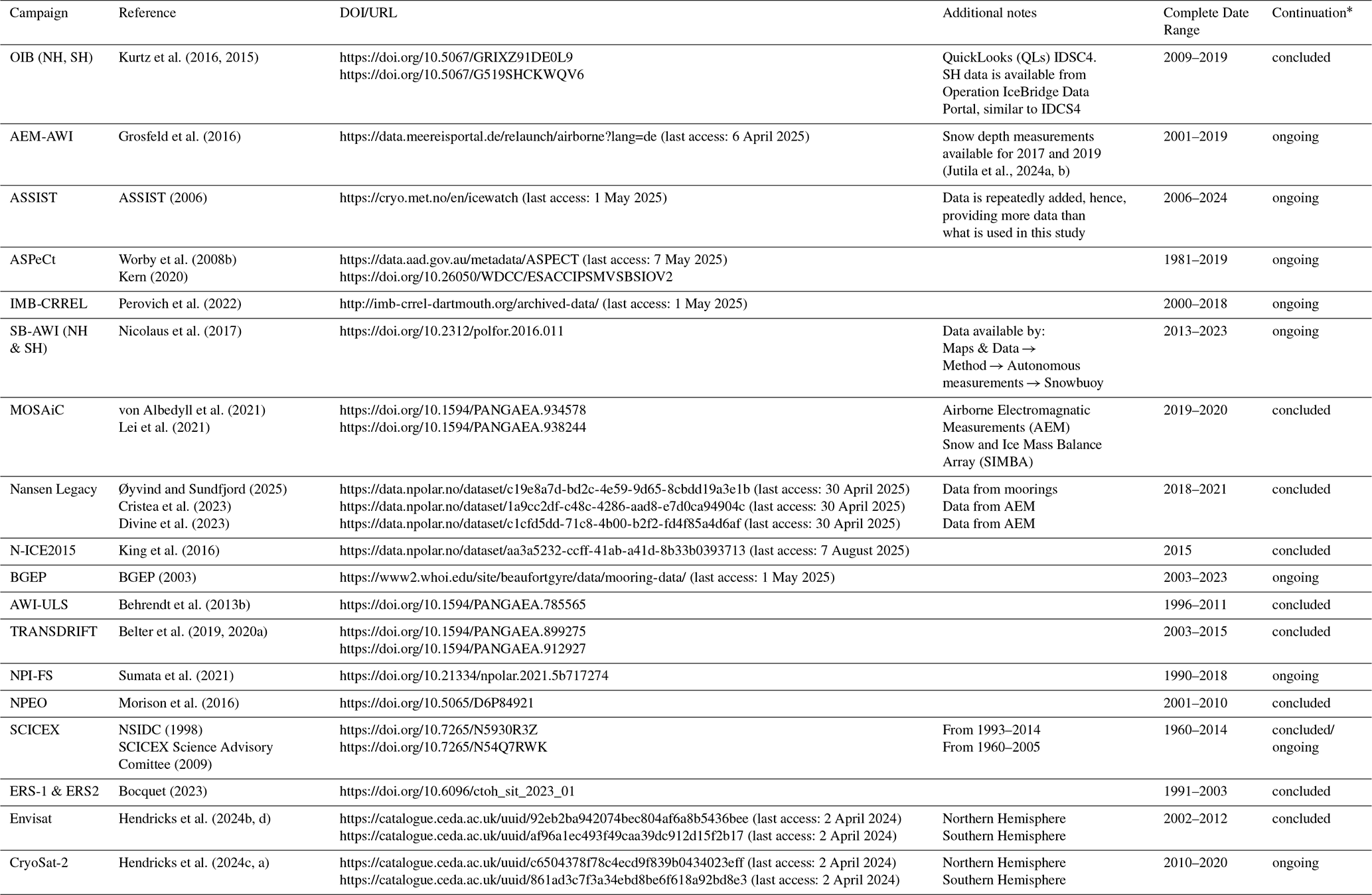
In total, data from 15 (see Fig. 4) different sources in the Arctic and 4 different sources in the Antarctic are included in the CCI SIT RRDP. Measurements are obtained from different platforms, that is, airborne, moorings, and autonomous drifting buoys, ships, and submarines, using a variety of methods. These methods and data products will be described more thoroughly in the following sections. A complete overview of the data sources used in the CCI SIT RRDP for both hemispheres is presented in Table 1 and links to the raw data are available from Table 2. Although some measurements were obtained as part of a concluded campaign, many measurements were continuously obtained and released once processed. This information is available in Table 2. Data sources are further illustrated in the Sankey diagram in Fig. 2, which shows the platform and measurement techniques, the names of the data sources and the associated geophysical sea ice variables included in the CCI SIT RRDP. From here on, the data sources will be referred to by their abbreviations as provided in Table 1.
Table 1Overview of reference measurements and their sources included in the CCI SIT RRDP for both the Northern (NH) and Southern (SH) hemispheres.
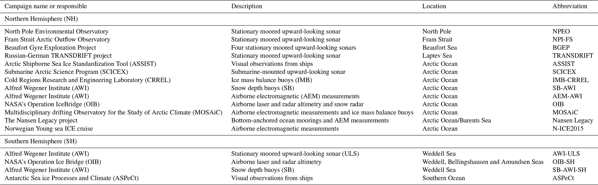
Table 2Direct data access is provided to all included reference data by using the DOI/URL links. DOI's are used when available. See footnotes for an explanation of the Continuation status.
* Ongoing: New data is repeatedly obtained and released when ready, concluded: No new data is expected to become available, ongoing/concluded: New data is not being obtained as a part of this project, but some data is still being processed for releaseability.
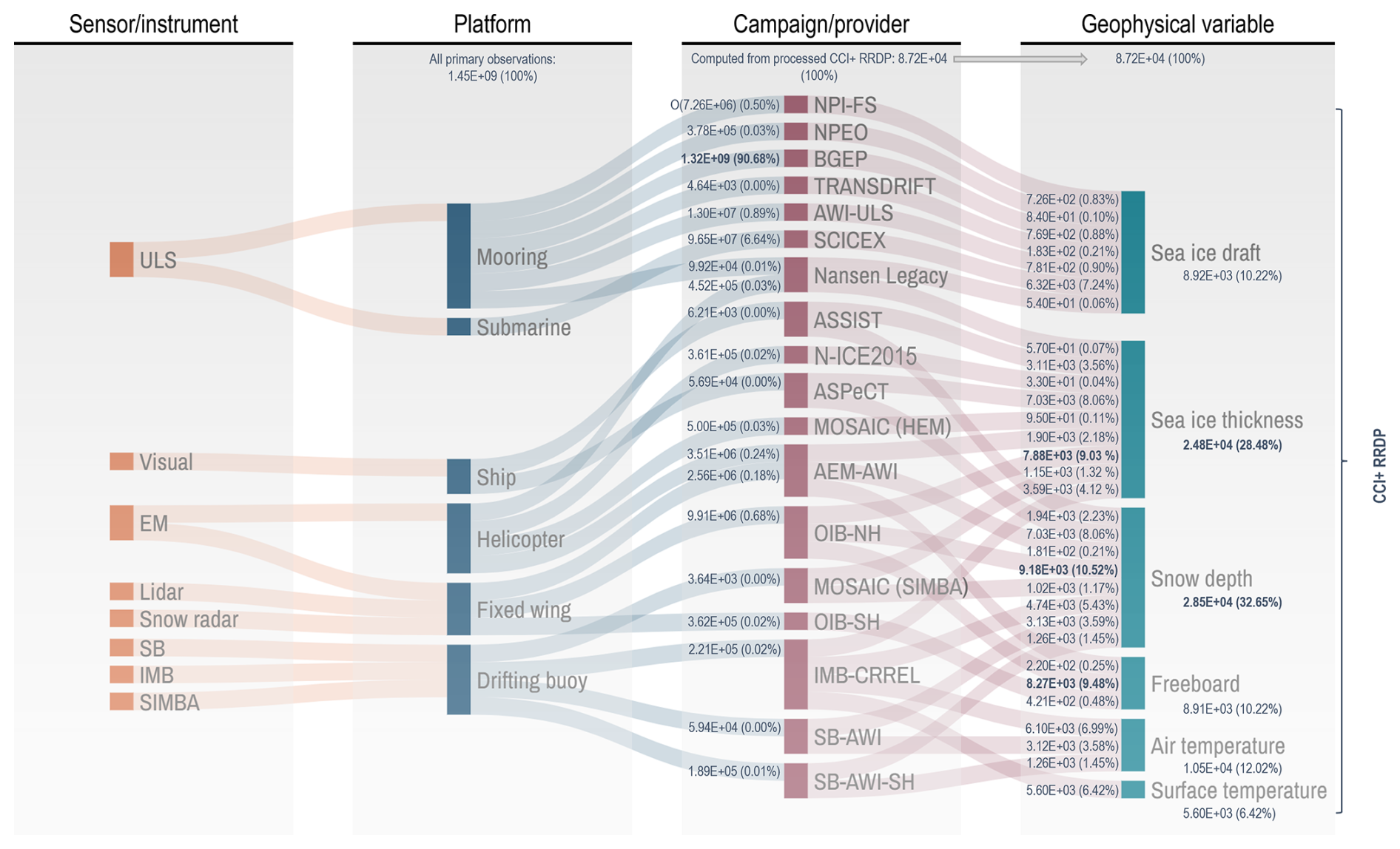
Figure 2Sankey diagram providing an overview of the data sources used in the CCI SIT RRDP and how they are acquired, by whom/when and what has been observed. The diagram is shown by four categories; sensor or measurement type, platform, campaigns (Table 2), derived geophysical variable, and their dependencies. We note that the data volume included in the CCI SIT RRDP is represented here by numbers (in scientific notation) and percentages, and it is dependent on the processing level. Platform data volume denotes raw data, while campaign/geophysical variables refer to processed data. Note that the highest contributing data sources (at different processing levels) are highlighted in bold, defined as the three highest contributing (in %) unless there is a large gap to the lesser contributors. In particular, the platform/mooring contributes more than 80 % of the data, which primarily reflects the large time series, high sampling frequency, and temporal coverage of the buoys. In contrast, campaign (OIB-NH, ASPeCt, or SCICEX) primarily reflect spatial coverage, since these numbers refer to the processed CCI SIT RRDP. In total, SIT and SD account for approximately 60 % of the CCI SIT RRDP. The notation O(number) denotes an approximation.
2.1 Airborne measurements
Measurements from OIB, AEM-AWI, MOSAiC, N-ICE2015 and the Nansen Legacy are conducted from airborne platforms, either fixed-wing aircraft or helicopters (see Fig. 2). These measurements provide a higher spatial resolution than satellite measurements, and a larger spatial coverage than in situ observations, however, they are usually temporally limited to a few days to weeks in specific months, primarily spring (March–April) in the NH and austral spring (October) in the SH, depending on when and whether an airborne campaign was conducted (see Fig. 5).
OIB's primary objective was to bridge the gap between NASA's ICESat (2003–2009) and ICESat-2 (2018–onwards) satellite missions. During its duration from 2009 to 2019, more than 12 different types of fixed-wing aircraft were used, and within this time period several updates to the instruments used for surveying were made. For a detailed overview of the instruments used for different periods, along with an impact assessment on the obtained data, see MacGregor et al. (2021). The OIB measurements used in this study consist of data from the IceBridge “L4 Sea Ice Freeboard, Snow Depth, and Thickness”, Version 001 (IDCS4), data product in the period of 2009–2013. Data after this are provided as quicklooks (Kurtz et al., 2016), which basically means that significantly less processing has been performed to provide a quick assessment of the collected data, leading to biases in the derived products, see Sect. 2.1.2. Quicklooks are processed from 2012–2019, but are only used from 2014–2019 due to IDCS4 being available until 2014. The measurands, that we compare to satellite observations are the sea ice FRB (total FRB subtracted the snow depth) and SD as well as SIT which is derived from laser and radar observations with additional sea ice density parametrisation. The officially published Antarctic campaign data are limited to total FRBs from the airborne topographic mapper (ATM) for the 2009 and 2010 campaigns, with no snow depth estimates provided and, hence, no sea ice thickness estimates. The sensors used to produce the OIB product, used herein, are the ATM laser altimeter system (Sect. 2.1.1), a digital camera (Sect. 2.1.1) and a snow radar (Sect. 2.1.2).
AEM-AWI, MOSAiC, N-ICE2015 and the Nansen Legacy measurements are conducted using an electromagnetic (EM) sounding device (known as the “EM-Bird”, see Sect. 2.1.3) dedicated to measuring the total ice thickness. In total, 33 campaigns are included in the AEM-AWI dataset as provided in Olsen and Skourup (2026a) along with information on the platform (either fixed-wing aircraft or helicopter) and measurement type for each campaign. AEM-AWI includes data from 2001–2019, but has not been measured consistently every year. For campaigns in 2017 and 2019, snow depth measurements (Sect. 2.1.2) were also obtained using an airborne frequency-modulated continuous-wave ultrawideband radar (Jutila et al., 2024a, b), which has been included in the CCI SIT RRDP. Additionally, total thicknesses from EM measurements were obtained during both the N-ICE2015 project (2015), the Nansen Legacy project (2019–2021) and the MOSAiC Expedition (2019–2020) using helicopters from ships, also termed HEM. MOSAiC HEM measurements were provided with quality flags, described in the data product user manual (von Albedyll et al., 2021). The following flags were used to filter the data QF_Reliability ≤ 2, Filter_Moderate_filter = 1 Filter_Strict_filter = 1. Total freeboards are provided for 2004 (IRIS, GreenIce) and 2007 (PolICE) campaigns in the AEM-AWI dataset (Olsen and Skourup, 2026a), derived from the EM-integrated laser.
2.1.1 Airborne topographic mapper (ATM) and digital camera
The main components of ATM are two conically scanning laser altimeters that measure the surface elevation along the path of the aircraft at 15 and 2.5° off-nadir angle, respectively (MacGregor et al., 2021). The ATM measures surface elevation relative to the WGS-84 reference ellipsoid by incorporating measurements from global navigation satellite system (GNSS) receivers and inertial navigation system attitude sensors. Measurements from ATM are subsequently converted to measurements of total freeboard by subtracting the instantaneous sea surface height (the local sea level obtained from lead measurements) from the measured elevation height. Determination of the sea surface height involves corrections of geoid height, tides, atmospheric pressure and the dynamic sea surface e.g. waves. During these procedures, information from the geo-referenced images from the digital cameras is used to support the identification of leads, which are used as tie-points for the instantaneous sea surface height. For more information about the ATM and the subsequent processing, see Kurtz et al. (2013).
2.1.2 Snow radar
SD is recorded using an ultra-wide frequency-modulated-continuous-wave (FMCW) radar working at either 2–8 or 2–18 GHz band (MacGregor et al., 2021; Jutila et al., 2022b). The snow radar measures the return radar signal as a function of time, which is scattered from the illuminated area below the aircraft. SD is determined by identifying the air-snow and snow-ice interfaces (see Fig. 1 for the definition of the interfaces) in the received signal and converting the time difference between these interfaces to SD, accounting for the slowdown of the propagation speed in snow, by using the refractive index of snow (Kurtz et al., 2013).
Several different data products are available from snow radars, which are primarily caused by the use of different re-trackers (methodology to identify the air-snow and snow-ice interfaces, as shown in Fig. 1). Within this RRDP, three different re-trackers are employed in the three different data products (IDCS4, QLs, AEM-AWI-SD).
-
IDCS4 (denoted NSIDC in K17). A full description of the algorithm is available from Kurtz et al. (2013), which utilises an empirical method that selects the air-snow interface either as the first significant peak above a defined threshold or the fit point when the rise in radar return power reaches a specified threshold, for the cases where no peaks are detected. The snow-ice interface is selected as the maximum in the radar signal below the air-snow interface.
-
QLs (denoted GSFC-NK in K17). The full details of the algorithm methodology are described in the product documentation at NSIDC, but are based on the waveform fitting method described in Kurtz et al. (2014). The algorithm fits a model waveform to the snow-radar data, and both interfaces are selected from the model fit results. The model fit is highly sensitive to the parameters used in the fitting process, where the most important include the initial guess and model fit bounds for the interfaces along with the maximum number of iterations.
-
AEM-AWI-SD. Jutila et al. (2022b) implemented a peakiness-based method, adapted from satellite radar altimetry, to enhance the detection of air–snow and snow–ice interfaces. This method is more robust in picking the right surface, especially when the air–snow interface is the dominant scattering surface, compared to, e.g., the Haar wavelet method. Their method is specifically tailored for the snow radar system deployed during the AWI IceBird campaigns, which has smaller footprints due to a lower flight altitude and slower speed of the aircraft.
According to Kwok et al. (2017), the QLs snow depth product exhibits a negative bias of approximately 5 cm compared to the IDCS4 product, based on comparisons with in situ measurements from the BROMEX and Eureka in situ field campaigns. Biases of similar magnitude (−4.5 to −6.7 cm) were found by King et al. (2015) and Petty et al. (2023) depending on sea ice type and settings (i.e., deformed ice versus level ice). The performance of the AEM-AWI-SD derived snow depth measurements for level, landfast first-year sea ice shows a mean bias of 0.86 cm between radar-derived estimates and ground truth (Jutila et al., 2022b). This aligns closely with the performance of the OIB IDCS4 product, which shows biases of 0.3 and −0.8 cm when compared to the same in situ observations as the QLs in Kwok et al. (2017). While alternative processing algorithms exist, their lack of consistency between datasets (Stroeve et al., 2020; Kwok et al., 2017) has led us to adopt a single approach in this study. However, this choice may introduce biases that exceed the uncertainties provided in the OIB QLs product, see Sect. 5.2.1.
2.1.3 EM-Bird
The EM-bird senses the distance of the sensor to the ice-water interface using frequency-domain EM induction sounding capitalizing on the substantial difference of electrical conductivity between the sea ice and snow layers compared to the ocean (Haas et al., 2009). Subtracting the instrument distance to the air-snow interface, measured by an integrated laser, from the distance to the ice-water interface yields the total (sea ice plus snow) thickness. The EM probe is towed by a helicopter or fixed-wing aircraft approximately 10–20 m above the surface of the sea ice. We further emphasize that helicopters tend to avoid certain ice types, such as thin or young ice, and open water areas for safety reasons, and therefore preferentially sample sea ice thicker than 0.30 m. Comparison with drill-hole data shows that helicopter-borne EM derived ice thicknesses agree within ±0.1 m over level ice (e.g., Haas et al., 2007). However, the ice thickness can be heavily underestimated over deformed ice (by as much as 50 % to 60 % in worst case) due to the footprint size of EM measurements over those 3D structures, and the presence of air pockets between the ice floes and blocks that have been pushed together (Haas et al., 2009, 2007; Mahoney et al., 2015).
2.2 Stationary moorings
In the CCI SIT RRDP, we have included data from stationary moorings equipped with upward-looking sonar (ULS) measuring the sea ice draft (the submerged part of the ice) from below the water (see Fig. 1). The ULS emits sound pulses and detects their echo return after being reflected from the bottom of the ice or from the water level between the ice floes. From these observations, the sea ice draft is derived using assumptions about seawater physical properties that influence the speed of sound, along with other corrections as described in Melling et al. (1995). ULS records are the only sea ice reference measurements, fixed to a specific geographic location, providing continuous measurements throughout the year. Although individual ULS measurements are essentially point observations when compared to satellite measurements, each observation has an effective spatial extent determined by the sonar footprint, which depend on the beam width of the sonar and the depth at which it is deployed. As an example, ULS's deployed about 50 m below the surface with a beam width of ∼ 1.8°, corresponds to a footprint of roughly 2 m at the ice–water interface (Krishfield and Proshutinsky, 2006). While the footprint size can influence the absolute draft estimate and its associated uncertainties, the continuous drift of sea ice over the moored instrument ensures that the ULS samples a representative range of sea ice conditions over a larger upstream area. This is especially true given the typical high sampling rate for ULS moorings (e.g. once per 2 s for BGEP, once per 19 s for Nansen Legacy, and between once per 1 min and once per 15 min for AWI-ULS). Moreover, the observed draft values and their variability depend not only on the actual sea ice thickness and its snow loading, but also on the averaging period, as well as the direction and speed of the sea ice drift. Many of the existing ULS's provide long time series (Fig. 4), and thus have the potential to provide reference measurements ideal for evaluation of long-term multi-satellite SIT CDRs.
In the Arctic, we include five sources providing stationary ULS data; the North Pole Environmental Observatory (NPEO) located at the North Pole with data from 2001–2010, the Fram Strait Arctic Outflow Observatory of the Norwegian Polar Institute (NPI-FS) located in the Fram Strait with data from 1990–2018, the Beaufort Gyre Exploration Project (BGEP) in the Beaufort Sea providing data from 2003–2023, the Nansen Legacy project providing data from 2019 to 2021, and the Russian-German TRANSDRIFT project (TRANSDRIFT) in the Laptev sea with data from 2003 to 2016. Where the NPEO, NPI-FS, BGEP and TRANSDRIFT (2013–2015) moorings are measuring using an Ice Profiling Sonar (IPS), the Nansen Legacy and TRANSDRIFT (2003–2016) are using upward-looking Acoustic Doppler Current Profilers (ADCPs) (Belter et al., 2020b). These different measurement techniques might introduce biases in the measured draft.
In the Antarctic, there are ULS draft observations from AWI (AWI-ULS) moorings in the Weddell Sea, where data were collected from 1990 to 2011. We note that currently there are several ULS stationed around the Arctic and Antarctic, ensuring the continuation of the mooring time series of the ice draft. However, data are not available in near real time as the sensor is submerged below the water. Routine efforts are required to deploy and retrieve the ULS data, which are then processed. Hence, the lag time for data collection is significant, often at least one year, compared to other data sources, e.g., autonomous drifting buoys equipped with Iridium link.
To our knowledge, there are no community practices w.r.t. direct validation of ULS derived sea ice drafts. However, different methods to derive the sea ice draft from the sound pulse runtime (or other) measurements can impact the resulting uncertainties, see Sect. 5.2.
2.3 Drifting buoys
Drifting buoys are autonomous systems, installed on selected sea ice floes, that drift freely with the ice compared to being anchored to one location as moorings. Depending on the buoy model, drifting buoys provide, along with other variables, the evolution of the thermodynamic growth and melt of the ice and/or changes in the snow depth at the specific point where they are deployed. The representativeness of the data acquired by these buoys depends on the initial snow and ice conditions at the time of deployment, as well as on how representative the selected ice floe is with respect to the surrounding ice cover. The derived information from drifting buoys is limited to the floe on which they are deployed, and thus represents a point measurement. With that a drifting buoy cannot capture the ice distribution on larger spatial scales or the changes in the ice thickness distribution due to deformation, unless they are deployed in an array. However, a drifting buoy allows us to monitor the temporal development of various ice and snow physical properties of that particular ice floe.
In the CCI SIT RRDP, we have included data from ice mass balance (IMB) buoys, maintained by the Cold Regions Research and Engineering Laboratory (CRREL) (Perovich et al., 2022), covering the period 2003 to 2018; the Snow and Ice Mass Balance Array (SIMBA) deployed during the MOSAiC expedition in 2019 to 2020; and dedicated acoustic snow depth buoys (SB) deployed by AWI during the time period 2013 to 2023. IMB-CRREL and SIMBA buoys are only available for the Northern Hemisphere, whereas SB data are available for both hemispheres. The data from IMB-CRREL for 2017 is found to be faulty, as all recorded values are identical. Consequently, these data were excluded from the CCI SIT RRDP.
The Snow and Ice Mass Balance (IMB) buoys measure the thermodynamic contribution to changes in the mass balance of sea ice. The main component is a thermistor string mounted vertically through the snow and ice column to measure the temperature profile, along with acoustic sounders placed above and below the ice, measuring the location of the air-snow or air-ice interface and of the water-ice interface, respectively. The combined snow + ice thickness is determined from the acoustic sounders and can be separated into measurements of SD and SIT by taking into account initial measurements of the snow/ice interface taken during deployment. Specifically, SD is given as the initial SD + snow accumulation or melt, while SIT is the distance between the top interface (air/snow or air/ice) and the bottom interface (water/ice) subtracted the SD (Planck et al., 2020). In addition, the buoys are typically equipped with a barometer and an air temperature sensor. From the IMB-CRREL buoys, we include measurements of SIT and SD, along with surface and air temperature. Typically, 3–6 IMB buoys are deployed each year in the Arctic Ocean, with the most regular deployments focused in the Beaufort Sea and at the North Pole with a typical survival period of 1 year (Richter-Menge et al., 2006a). The time interval between subsequent mass balance data measurements (SD and SIT) varies for different buoys and depends on the buoy model and the year of deployment. In general, the mass balance data are measured approximately every four hours for the majority of buoys, but several buoys provide measurements every two hours and some (2002A, 2003A) only twice a day, while others (2015I, 2015J, 2015K, 2018A, 2018B, 2018C, 2018D, 2018E) have measurements every hour. SIMBA is a thermistor string type IMB (Lei et al., 2021) and therefore also measures vertical temperature profiles through the air-snow-ice-water column using a thermistor string. During MOSAiC 22 SIMBA buoys were deployed in the Arctic Ocean in a Distributed Network (DN).
As such, an individually deployed IMB buoy (IMB-CRREL) provides spatially localized measurements, due to its fixed position on an ice floe, but with relatively high temporal resolution. Whereas, an array of IMB buoys (SIMBA) is expected to better represent a larger spatial variation of ice thicknesses and snow depths on the scales of the array, while keeping the high temporal sampling. Automatic detection of snow depth and ice thickness from SIMBA has been evaluated against in situ data by Liao et al. (2019) when deployed in landfast ice (in the vicinity of Zhongshan station in Prydz Bay, East Antarctic). In situ snow depth and ice thickness were measured on a weekly basis, where boreholes were drilled through the ice and the distance was measured using an ice gauge to determine ice thickness. Snow depth was measured with a stainless ruler from three close (less than 1 m) random sites near the ice boreholes (within 2 m). Accuracies between observations from SIMBA buoys and in situ measurements are 0.01 and 0.005 m for ice and snow measurements, respectively. However, these accuracies represent an idealized scenario, as deformation is not taken into account and snowfall events may be limited. In reality, the accuracy of SIMBA buoys over sea ice is expected to be lower. No in situ comparison was recorded over drifting ice. Cheng et al. (2020) compared SIMBA observations acquired on a frozen lake in Finland, where estimates of snow depth and ice thickness, derived from automatic or manually identified air-snow, snow-ice, and ice-water interfaces in temperature profiles, were compared with in situ observations acquired from the lake at observation sites 500 m apart. Comparisons of (total) ice thickness record a bias of 0.04–0.06 m and RMSE of 0.13 m.
The IMB-CRREL and SIMBA buoys' initial thicknesses, i.e., the ice thickness at deployment, are shown in Fig. 3. Of the 92 IMB-CRREL buoys included here, only two buoys (2015H, 2018D) have an initial SIT < 0.5 m. In general, they tend to be deployed in ice thicker than 1 m with few exceptions (2003C, 2013A, 2015H, 2015I, 2015K, 2018D and 2018E) with 37 of them deployed in the perennial sea ice cover (MYI) with initial thicknesses > 2 m to decrease the likelihood of damage to the buoy due to e.g., sea ice deformation events and thereby prolonging its potential life span. Post-2009, more buoys are deployed in ice with an initial thickness < 2 m (44 out of 63) with a minimum initial thickness of 0.19 m (2018D), i.e., in the seasonal ice cover (FYI). This is consistent with the design of the first IMBs to be adapted and well-suited for deployments in MYI (Richter-Menge et al., 2006b). An optimized buoy design to better fit deployments in seasonal ice zones was first tested in 2009 according to Polashenski et al. (2011). Basically, all 19 SIMBA buoys (except 2019T79) were deployed in ice with initial thickness < 2 m.
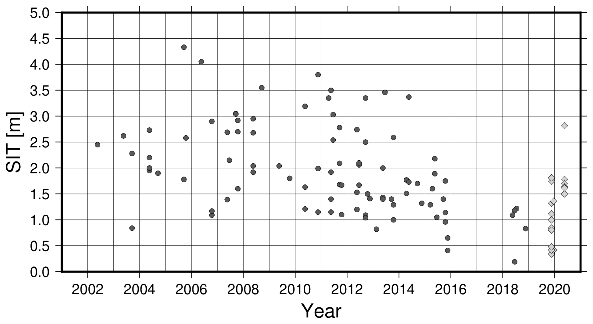
Figure 3Initial thickness for the 92 IMB-CRREL (dark grey dots) and 19 SIMBA (light grey diamonds) buoys included in this study.
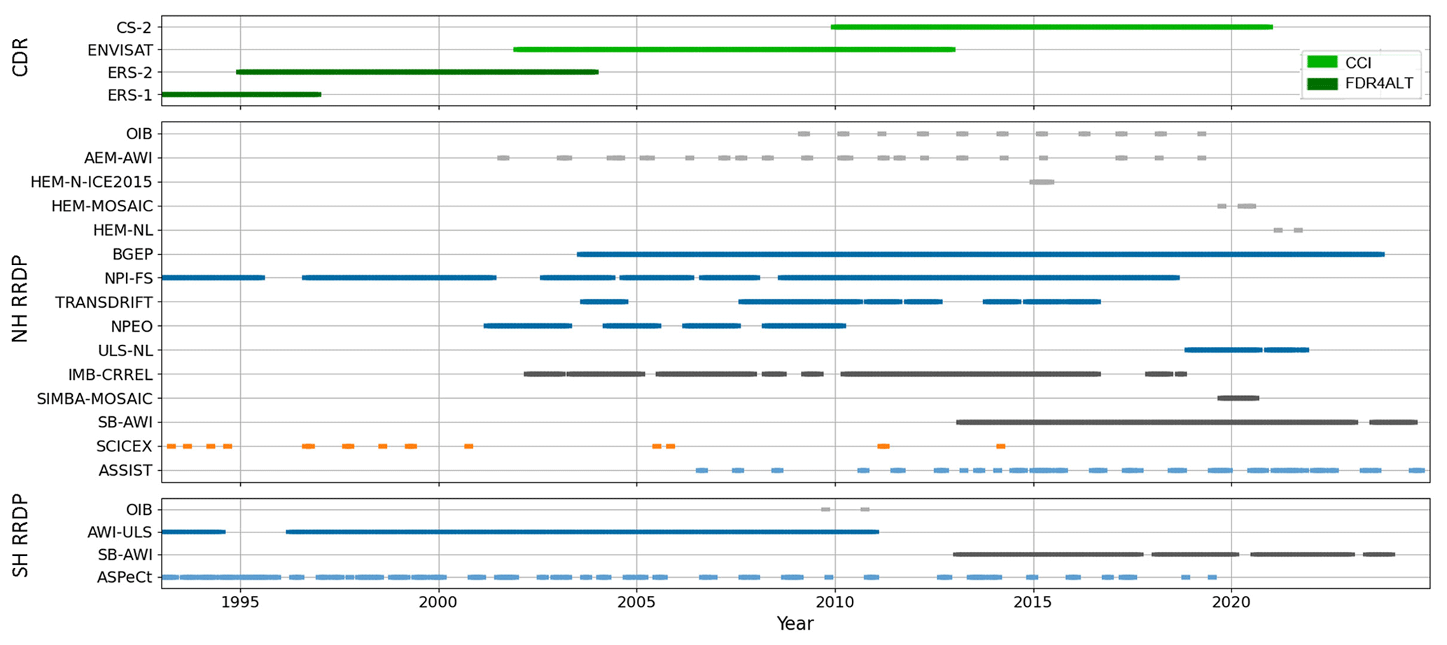
Figure 4Timeline of all data included in the CCI SIT RRDP. The CDR observations are color-coded according to project as shown in the legend, whereas the colors of the RRDP reflect the type of reference observations as defined in Fig. 5.
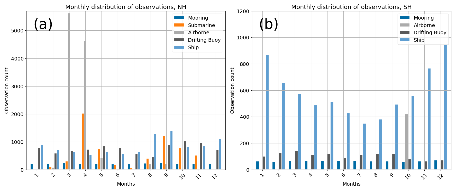
Figure 5Seasonal distribution of reference data in CCI SIT RRDP; (a) NH and (b) SH categorised based on sensor type.
Snow depth buoys (SB) measure relative changes in snow height, i.e. the accumulation of snow since deployment. These are then calibrated against the initial snow depths measured during deployment in order to retrieve the absolute snow depth values. In the Alfred Wegener Institute snow depth buoys (SB-AWI) (Nicolaus et al., 2017), the measurements are made with four ultrasonic snow depth sensors that are installed on a mast-attached platform. SB-AWI measurements are available for both hemispheres. The data transmission interval for SB-AWI is approximately once per hour, resulting in spatial and temporal characteristics similar to IMB-CRREL. We were not able to identify validation studies where the derived snow depths were inter-compared with in situ data, however, the SB is consistently deployed by AWI in both hemispheres, and has shown reasonable accumulation rates (e.g., Nicolaus and Katlein, 2017; Nicolaus et al., 2021; Arndt et al., 2024). Also, the methodology to convert the snow accumulation measurement by the buoy into a snow depth value is continuously developed further, especially for the Southern Ocean, including consistency checks to regional in situ measurements of the snow depth and consideration of the formation of snow ice and meteoric ice (Arndt et al., 2024).
2.4 Ships
Collected and archived ship-based observations are provided via the Ice Watch program (Hutchings et al., 2018) for the NH. The Southern Hemisphere has a corresponding program called ASPeCt (Antarctic Sea Ice Process and Climate), which was established in 1997 by the Scientific Committee on Antarctic Research. These are manual visual observations from the ship's bridge carried out by voluntary, ideally trained observers. Observations shall be recorded with the ASSIST (Arctic Shipborne Sea Ice Standardization Tool) following an Ice Watch protocol established in the 2000s in the NH and following the ASPeCt protocol in the SH. Reported observations shall include, for the three dominant ice thickness categories within a 1 km/1 nm radius around the ship, e.g., sea ice concentration, sea ice thickness, snow depth, stage of growth or melt, state of the snow cover and surface roughness. Despite the used protocols, the number of observed variables reported is often inconsistent and can vary between ship cruises. Factors influencing the quality of these observations are visibility around the ship, and experience and qualifications of the observers which cannot be quantified (find a brief description of Ice Watch instructions for observers in Sect. 3.1.2). ASSIST data is available from 2006–2024 and contains data from 89 voyages. Data until 2005 is available from the ASPeCt data archive and contains data from 83 voyages for the period 1980–2005. More recent additions (2002–2019) to the dataset have been processed and are publicly available (Kern, 2020). Links to data sources for ASPeCt and ASSIST are available from Table 2.
We are not aware of any specific validation practices that compare visual ship observations with other complementary data, especially with respect to SIT and SD. However, new techniques are emerging such as the Sea Ice Monitoring System (SIMS, von Abedyll et al., 2024) and downward looking cameras mounted on ships. Ship observations are, in a similar manner as the airborne campaigns, dedicated to individual cruises with a duration of 1–2 months. Thanks to the more harsh conditions during winter in the respective hemisphere, more ship-based observations can be found for the summer months (Kern et al., 2019). In general, ships, whenever possible, tend to avoid well-consolidated and deformed ice to limit risks, which impacts the ice observations. While estimates of the sea ice concentration are less influenced by this tendency to operate in easily navigable ice conditions, estimates of sea ice thickness and snow depth on sea ice are known to be biased low; thick and deformed ice conditions are underrepresented (Worby et al., 2008a). The ASPeCt and ASSIST data are included in this compilation to examine whether they can be used for sea ice thickness and snow depth comparisons to satellite altimetry, given their spatial and temporal coverage. These datasets are among the most extensive observational records available in the SH and also provide summer sea ice thickness measurements in the NH (Fig. 5), which may help fill observational gaps if they prove useful for this purpose. While differences in measurement techniques and associated uncertainties exist, their inclusion offers spatial context and qualitative insights that may complement other sources and support broader interpretation of sea ice conditions.
2.5 Submarines
The submarine dataset provides ULS SIDs, similarly to stationary moorings, except that the measurements are taken along trajectories and thus have a larger regional coverage. However, the data is collected only during dedicated cruises of 1–3 months duration. The submarine cruises are primarily military operations, which can imply that the data distribution to the common sea ice community can take several years due to restrictions on data sharing. The data included here were collected by the U.S. Navy and Royal Navy and are available for the Arctic Ocean. The temporal span of the data is from 1 February 1960 to 30 November 2005, along with data available in 2011 and 2014. Data from several other years (2012, 2016, 2018 and 2020) are currently being processed and evaluated for releasability. Examination of SCICEX data from the 2014 New Mexico cruise reveals anomalous behavior when compared to data from other years. Additionally, according to the SCICEX data product user manual (SCICEX Science Advisory Comittee, 2009), the 2014 New Mexico dataset has undergone an unspecified level of processing. Given these issues, the 2014 data have been excluded from the analysis, as it is likely not comparable with the other submarine measurements.
3.1 Pre-processing of reference data
All reference measurements underwent pre-processing before being converted to common spatial and temporal scales for comparison with satellite-altimetry-derived composites. In most cases, the necessary pre-processing steps involved converting the date and coordinate formats to the desired output format and/or automatically extracting location and/or date information from the file header, which are all considered standard procedures. Additionally, observations were filtered to exclude data points that potentially represent outliers. Specifically, measurements were removed if SIT exceeded 10 m, SD exceeded 2 m, SID exceeded 8 m, FRB exceeded 2 m, or if any variable had values below 0 m. In addition, several subsets needed additional pre-processing steps due to, e.g., incomplete information of time and/or position. As a result, a pre-processing (pp) flag is included in the final data file, indicating whether the data required additional pre-processing steps, which could be associated with higher uncertainties. As the required level of additional pre-processing varies for the different types of reference measurements, an overview of the use of the pre-processing flag is presented in Table 4. It should be noted that, because the data are subsequently averaged into monthly means on a 25 km grid for the Northern Hemisphere (NH) and a 50 km grid for the Southern Hemisphere (SH), temporal uncertainties of up to 24 h are expected to have minimal impact. Discussions of temporal and spatial representativeness are presented in Sects. 4, 7.6 and 7.7. In the following subsections specific major processing steps are further detailed.
Table 3Description of reference data structure in CCI SIT RRDP.
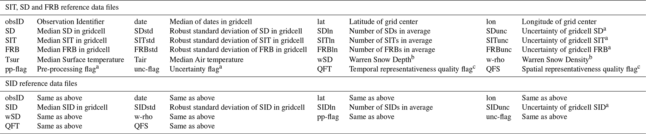
a See Sect. 5 for a description of how uncertainties are determined for each campaign b from Warren et al. (1999), c see Sect. 4.
Table 4Description of pre-processing flag (pp-flag) implementation.
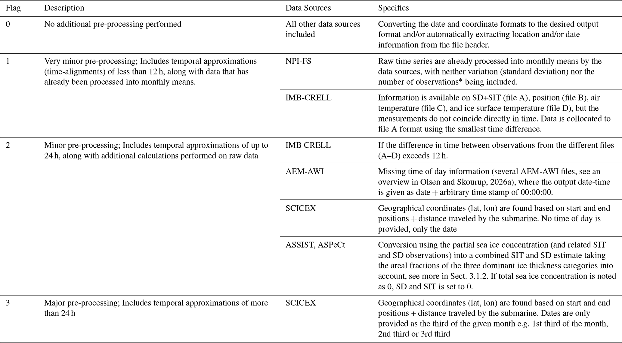
* An updated version of the data (Sumata, 2022) contains an estimate of the number of samples per observation given as in the order of 104 for data obtained with the ES300 instruments (until September 2006) and in the order of
106 for data obtained with the IPS4/5 instruments. This information has been added to the CCI SIT RRDP, but users should be aware that the number is an approximation.
3.1.1 AEM-AWI
Files within AEM-AWI either contain measurements of total FRB or total thickness (in combination with SD for files in 2017 and 2019). It was therefore decided to split the final product into two files, one with all the measurements of total ice thickness and one with all measurements of total freeboard (see Appendix in Olsen and Skourup, 2026a for a filewise overview).
3.1.2 Ship measurements
The IceWatch manual provides guidelines for observing SIT and SD from ships. The standard procedure requires making observations every hour while the ship is in motion. The ice is observed, depending on actual visibility conditions, up to 1 km/1 nm from the ship during a 10 min observation period, which is usually performed on the bridge of the ship. Recent instructions (https://aspectsouth.org/wp-content/uploads/2024/06/sea-ice-cards_LOGODOI.pdf, last access: 23 May 2025) reiterate that observations should be made every hour and recorded on the hour. Observers are required to document the sea ice types/classes and estimate their area coverage within a 1 km/1 nm radius of the ship, estimated from the radar display on the bridge of the ship. In addition SIT estimates are made by visually assessing overturned sea ice viewed from the bridge referenced to a 55 cm diameter buoy on the side of the ship, or a ruler/stick with 0.2 or 0.5 m graduation sticking out perpendicular to the side of the ship. Rafted ice is included in the thickness estimate, whereas ridged ice shall be excluded. The same measurement methodology is applied for SD, which is differentiated from ice by color.
The aim is to classify up to three dominant ice types or classes that together cover the largest area. These are denoted as primary, secondary, and tertiary ice, where the thickest ice type is primary, and the thinnest is tertiary. The areas of primary, secondary, and tertiary ice are summed to obtain the total ice concentration (Hutchings et al., 2018).
Due to the acquisition method, data from ASSIST and ASPeCt must undergo pre-processing to combine the observations of the individual ice types into one. The thickness and partial concentration of each ice type are used to make a weighted average of the mean sea ice thickness within the observed area (Hutchings et al., 2018). The following formulas show the computation of such averaged sea ice thickness estimates:
Here, P, S and T stand for primary, secondary and tertiary, respectively. Ctot is the total ice concentration, and CP, S, or T denote the ice concentration of the particular ice type. The combined SD is derived using the same weighting principle.
We use these reference measurements only if the sum of the partial concentration adds up to the total concentration and at least one of the partial concentrations belonging to SIT/SD is defined (e.g. is not NaN).
3.1.3 Submarine measurements
SCICEX submarine measurements were collected over an extended period, from 1960 to 2014. During this time period, the information provided in the data acquisition files is not consistent, and post-processing of different parts of the data has been treated by different institutions, which results in inconsistencies between different cruises. Nevertheless, as all SCICEX data are subject to some level of interpolation, due to a lack of continuous measurements of time and position, all data are given pp-flags in categories 2 or 3 (see Table 4).
Parts of the SCICEX data are known as the “analog subset” because it was derived from traces on paper rolls (SCICEX Science Advisory Comittee, 2009, see General resources Documentation for G01360 Analog Subset). Each file in the analog subset contains sea ice drafts of one line segment and provides only the start and end coordinates, along with date information including the year, month and the segment of the month in which measurements were obtained, given as the first, second, or third part of the month. We are using the following date-time conversion for converting the segment of the month into a date containing day and time:
-
1st third = Day 5 at 00:00:00 UTC
-
2nd third = Day 15 at 00:00:00 UTC
-
3rd third = Day 26 at 00:00:00 UTC
Other files within SCICEX provide a specific day of the month, and for these, we use the specified day and an arbitrary time at 00:00:00 UTC.
Spatial interpolation to obtain the positions of each reference measurement is done using the inverse haversine formula from the Python package haversine 2.8.0 (released 28 February 2023). Here, the coordinates (ϕ, λ) are calculated iteratively using the distances (δd) provided between observations when available and the bearing (θ) between neighboring points. When these are not available, an equal distance is assumed between subsequent measurements using the start and end positions.
3.2 Transformation into composites for comparison with satellites
Reference measurements were averaged to the Equal-Area Scalable Earth Grid in version 2 (EASE2) provided by the National Snow and Ice Data Center (NSIDC). For each gridcell, the median was used to compute the average value, accompanied by the corresponding robust standard deviation (see Eq. 5). The date assigned to each gridcell corresponds to the median date of all observations within that gridcell. The median and robust standard deviation were selected to reduce the influence of outliers and to better handle skewed distributions present in several datasets. This approach was preferred over the mean and ordinary standard deviation to obtain a typical representative value for each grid cell. Using the median date also indicates when the reference measurements are most densely distributed and enables matchup weighting based on temporal distance. EASE2 is based on a polar aspect spherical Lambert Azimuthal equal-area projection (Brodzik et al., 2012) and the WGS-84 reference ellipsoid. The NH grid dimension is 5400 km × 5400 km with a spatial resolution of 25 km, resulting in a grid consisting of 432 × 432 grid cells, whereas the SH grid has a spatial resolution of 50 km, resulting in a grid consisting of 216 × 216 grid cells. The grid is centered on the geographic pole, which means that the pole is located at the intersection of the center cells. A temporal resolution of 30 d is used for both hemispheres. Data obtained from stationary moorings have only been temporally averaged, as these are fixed in space. The output data was subsequently sorted temporally and processed into a standardized text format, as shown in Table 3. Since most campaigns only record some of the information required by the standardized format, missing values were filed as NaNs.
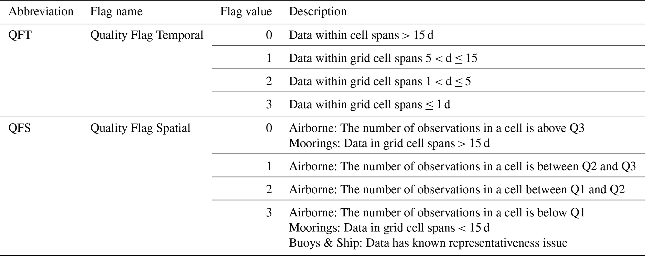
We further flag (“quality-flag” or QF) data according to their temporal and spatial representativeness. This is achieved by separating the flag into two categories: a temporal representativeness flag (QFT) and a spatial representativeness flag (QFS), see Table 5 for specifications. Spatial representativeness (QFS) is difficult to assess, particularly given the different nature of reference measurements. To address this, the reference measurements are divided into categories based on how they are measured. Airborne measurements (OIB, AEM-AWI, N-ICE2015 and parts of the MOSAiC and the Nansen Legacy) and submarine measurements (SCICEX) operate above/below the ice, respectively, and have distinct footprint sizes. Consequently, the number of observations within a grid cell scales with the area covered. Due to the different footprint sizes, particularly for airborne and submarine measurements, the spatial representativeness is estimated by the number of measurements within a grid cell. Four flag values are defined based on the 25 % (Q1), 50 % (Q2) and 75 % (Q3) quartiles of the total number of observations across the dataset. These spatial flags provide a relative indication of area coverage compared to the overall data distribution. For more advanced considerations of the scaling properties related to, e.g., OIB data, we refer to (Xu et al., 2020). In contrast, buoys placed on the ice have an inherent issue with spatial representativeness due to their fixed location on the ice floe. Thus, by definition, these have limitations in terms of high spatial representativeness. Similarly, ships navigating in ice tend to choose a route with thinner sea ice and, therefore, exhibit a sampling bias because only a part of the SIT and SD distribution function can be covered. In addition, any ship-based and airborne reference measurements are likely to be biased to represent spring/summer sea ice conditions; this applies in particular to OIB. In contrast, moorings, although fixed in position beneath the sea ice, can achieve high spatial representativeness due to the drifting ice passing over them, provided that different ice masses drift across. As such, their spatial representativeness can be approximated by the number of days with measurements in a given month.
Table 5Quality flags to deduce representativeness of the reference measurements. Note that QFT thresholds are based on the monthly temporal resolution produced within the RRDP, and would need to be updated for users that utilise a different spatial resolution when processing with this set-up.
All source reference data in the CCI SIT RRDP are associated with some level of uncertainty; however, except for OIB, they lack uncertainty information for individual data points. Instead, uncertainty quantification in the CCI SIT RRDP must rely on average errors, accuracies, or uncertainties reported in various studies. These sources are presented in Table 7 along with the estimated uncertainty. It is important to note that the amount of uncertainty information varies greatly among the datasets. Several uncertainty estimates are based on assumptions (e.g., AEM-AWI), rely solely on instrument accuracy (e.g., IMB-CRREL), or are only valid within a certain range. Therefore, an uncertainty flag is introduced to quantify the level of variability available in the uncertainty estimate (see Table 6). Whereas this flag serves as an indicator of the confidence we have in the uncertainty estimate, it does not take into account issues regarding temporal and spatial representation errors. These are quantified in the quality flags described in Sect. 4 and examples of the impact of the flags are provided in Sect. 7.6.
Table 6Uncertainty flag describing the expected quality of the uncertainty estimate (level of variability and whether it seems reasonable). Does not take into account issues with representativeness. This is quantified by the quality flag (see Table 5).
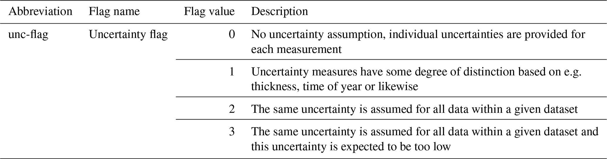
Section 5.2 provides a description of the uncertainty associated with each type of reference measurement, including the assigned uncertainty flag values. An overview of the uncertainty flags is presented in Table 6, and Table 7 lists the uncertainties and the corresponding uncertainty flags for all datasets.
Kurtz et al. (2016, 2015)Haas et al. (2007)Jutila et al. (2022a)Haas et al. (2007)Haas et al. (2007)Haas et al. (2007)Worby et al. (2008a, 1999)Worby et al. (2008a, 1999)Perovich et al. (2022)Richter-Menge et al. (2006a)Lei et al. (2021)Lee et al. (2015)Nicolaus et al. (2021)Krishfield and Proshutinsky (2006)Behrendt et al. (2013a)Belter et al. (2020b)Belter et al. (2021)Sumata (2022)Morison et al. (2016)Rothrock and Wensnahan (2007)NSIDC (2006)Table 7Uncertainties related to the products in CCI SIT RRDP.
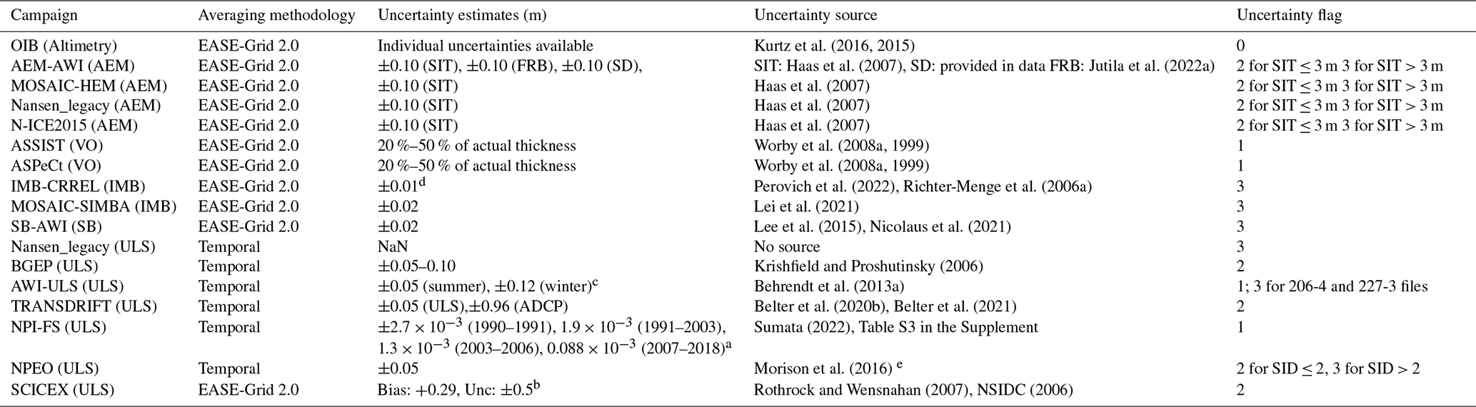
VO: Visual Observation, a Uncertainty of the monthly means Table S3, b uncertainty based on 2⋅ std, c default: line correction for sound speed model: ±0.23,
d 0.01 m accuracy in usual conditions 0.02 m if it is very cold, e uncertainty estimate available from metadata.
Another concern is the interchangeable use of terms such as error, uncertainty, and accuracy, despite their distinct statistical meanings. The error represents the absolute deviation between the measured and true values, the precision describes the closeness of the agreement between the measured and the true values, and the uncertainty provides a quantification of the doubt of a measurement given as an estimate of the range within which the true value is expected to lie (Taylor, 1939; Bell, 1999). Therefore, while error is calculated based on a known true value, uncertainty is typically described by a confidence interval or standard uncertainty within which the true value is expected to fall. Uncertainty is a measure of the random error in a sample, while systematic error is termed bias or offset (Bell, 1999). Based on these definitions, when a paper refers to an error indicated by a value ±, it is interpreted here as uncertainty.
5.1 Uncertainty propagation in average calculation
The propagation of uncertainties in the final CCI SIT RRDP product is based on the principles outlined in Taylor (1939). According to Taylor's theorem, if the uncertainties of the measurements x1 to xn are independent and random, then the uncertainty of the mean is obtained by summing the individual uncertainties in quadrature and dividing by the square root of the number of measurements (N).
The upper bound of the uncertainty is the ordinary sum of the measurement uncertainties:
In this study formula (6) is used for the propagation of uncertainties, hence, the uncertainties are assumed to be independent and random, as we do not have sufficient information to obtain full error covariance matrices. Nevertheless, this is not necessarily the case, and it can result in an underestimation of uncertainties. This effect is most pronounced for reference measurements with a large number of observations per grid cell, particularly for the ULS data, where several thousand measurements are averaged to obtain the final values in the CCI SIT RRDP. Therefore, we underline that it might be more appropriate to use the upper bound uncertainty in some cases, which is equivalent to the uncertainty estimates shown in Table 7. This is especially true for reference measurements, where we have the same uncertainty estimate for all input data (equivalent to an uncertainty flag of 2 or 3), as is the case for the majority of the data from airborne campaigns or SID measurements. Table 7 presents a summary of the input uncertainty estimates for each campaign, along with a citation to the publication, where the uncertainty estimate was originally sourced. In the following sections, we describe in more detail how the uncertainty estimates of each campaign are obtained and the underlying assumptions.
5.2 Original uncertainties of data
5.2.1 Airborne data
OIB data contain individual uncertainty estimates for FRB, SD and SIT measurements as the only data source included in the CCI SIT RRDP. These uncertainties are based on variations in the sea ice properties, instrument, and inter-campaign algorithm changes. As individual uncertainties are provided, the OIB data have been given an uncertainty flag of category 0. A detailed overview of how uncertainties are calculated is presented in Kurtz et al. (2013). A central concern of this approach is the substantial variation in both the magnitude and interannual variability of snow depths among different OIB-derived datasets; see Sect. 2.1.2. In particular, the OIB QLs are prone to bias low (−4.5 to −6.7 cm) depending on sea ice type and settings (i.e., deformed vs. level) (Kwok et al., 2017; King et al., 2015; Petty et al., 2023). These magnitudes might exceed the uncertainties provided in the OIB data products, which complicates our efforts in establishing a consistent uncertainty estimate based on the uncertainties provided in the products.
The uncertainty of AEM/HEM (AEM-AWI, MOSAiC, N-ICE2015 and Nansen Legacy) measurements depends on the sea ice conditions i.e., whether the ice is level or deformed, as described in Sect. 2.1.3. For airborne EM measurements, we here adopt a constant uncertainty of ±0.1 m over level ice. Since this uncertainty is not representative for deformed ice and, to the best of our knowledge, no uncertainty quantification has been estimated for it, further analysis is needed. Here, we introduce an uncertainty flag of category 3 for average sea ice thicknesses greater than 3 m, while sea ice thinner than 3 m is assigned a category 2 uncertainty flag. In principle, level ice can exceed 3 m, and deformed first-year ice can be thinner than 3 m. Therefore, using this threshold may introduce some erroneous assumptions affecting the results. However, since we lack detailed information whether the ice is level or deformed, this represents a first approach to flag the data based on these parameters. The total FRB measurements are related to an overall uncertainty of ±0.1 m (Haas et al., 2007) and are given an uncertainty flag of category 2. Snow depth measurements are also linked to a fixed uncertainty of ±0.1 m, which is provided in the source data.
5.2.2 Stationary moorings
Although individual moorings have their own uncertainty estimates, the cause of uncertainty for observations obtained by similar measurands tends to be similar. Raw ULS measurements can be linked to significant biases caused by measuring the first return that comes from the ice closest to the sonar, which can cause draft values for deformed ice to be overestimated. They are also prone to uncertainties linked to e.g., corrections for variations in local atmospheric pressure, instrument tilts, and variations in the speed of sound in the water column (BGEP, 2003). However, all mooring data used in this validation study have undergone some quality assessment with corrections applied to decrease uncertainties and biases if deemed appropriate by the data providers.
BGEP and TRANSDRIFT data have undergone significant processing, resulting in no expected bias and an uncertainty in the range of ±0.05–0.1 m for BGEP and ±0.05 m for ULS data from TRANSDRIFT.
As previously mentioned NPI data was already processed into monthly averages (using the mean) and therefore the uncertainty used in this dataset is based on the uncertainties of the monthly average SIT product, which was created based on the monthly average SID, see Sumata (2022). In the supplementary materials of this publication (Table 3) are listed four categories of uncertainties for the SIT based on a mix of instrument type (ES300 or IPS4/5) and on the year. The uncertainties vary between ±2.7 × 10⁻³ and ±0.088 × 10⁻³ m. Due to the lack of uncertainty estimates for the NPI SID data, these SIT uncertainties are applied to the NPI SID dataset. Since the NPI uncertainty estimates vary with sensor type and instrument age, an uncertainty flag of category 1 is assigned. The upward-looking ADCP data from TRANSDRIFT have a significantly larger uncertainty of ±0.96 m, which is a consequence of the general nature of the ADCP instrument setup designed to measure the velocity fields within the water column rather than to derive SID (Belter et al., 2021). NPEO has also undergone corrections that result in an estimated uncertainty of ±0.05 m for level and gently undulating ice, but no additional correction has been made to correct for the first return (Morison et al., 2016). Therefore, SID of deformed sea ice may tend to be biased high. A similar first-return–related bias may also affect other SID measurements where equivalent corrections have not been applied. To account for this, we assign an uncertainty flag of category 3 to monthly averaged NPEO SID values that exceed 2 m. Sea ice draft from ADCP's from the Nansen Legacy has no quantified uncertainty. Furthermore, the provided uncertainty for the TRANSDRIFT ADCP's cannot be used, as a major contributor to the TRANSDRIFT ADCP's uncertainty is the lack of reliable measurements of pressure, which is not the case for Nansen Legacy ADCP's. Due to this, the Nansen Legacy SID measurements are given an uncertainty of NaN and an uncertainty flag of category 3.
The mooring data for the SH from the AWI-ULS dataset have undergone varying levels of processing, and the estimated uncertainty depends on both the time of the year and the applied corrections. Based on Behrendt et al. (2013a), SID corrected by zero-line correction have an estimated uncertainty of ±0.05 m in summer (November to May) and ±0.12 m in winter (June to October). When using the sound-speed model instead of zero-line correction, the estimated uncertainty is ±0.23 m. Here we decide to use the zero-line correction result when available, as Behrendt et al. (2013a) found only a few cases where the sound-speed model performed better than the zero-line correction. SID data from moorings 206-4 and 227-3 are given an uncertainty flag of category 3, as Behrendt et al. (2013a) states that these moorings have problems with the pressure sensor, signifying that they have undergone a simpler and likely less accurate correction.
Behrendt et al. (2013a) also find significant biases for AWI-ULS drafts, as the measured drafts are consistently overestimated, except when measuring on completely level ice. The bias depends on the SID measurement and ice type, with MYI summer having smaller biases of around 0.3 m, whereas FYI winter has the largest biases, ranging from 0.42 m for ULS instrument depths of up to 100 and 0.68 m for ULS instrument depths up to 180 m. However, these biases were computed for the Arctic, and since sea ice in the Antarctic is generally younger and thinner due to e.g., differences in ocean heat flux and thermal insulation from a thicker snow cover (Maksym et al., 2012; Haas, 2016), they may not be accurate.
5.2.3 Drifting buoys
IMB-CRREL drifting buoys lack information regarding the uncertainty of the data after processing. However, information about the estimated instrument accuracy of the acoustic rangefinder sounders is provided. Therefore, this information is utilized as the uncertainty for each measurement. According to Richter-Menge et al. (2006a), the acoustic rangefinder sounders, which are located above the air-snow/ice interface and below the water-ice interface, have an accuracy of 5 mm, resulting in a combined uncertainty of 0.01 m, when summed. However, this value is likely underestimated when compared to satellite measurements, as IMB-CRREL buoys provide localized data. Although the standard deviation of the final measurements in CCI SIT RRDP accounts for some variability, each buoy is positioned and follows its own drifting ice floe, and thus the impact of the overall variability of the ice in the area is expected to be largely unaccounted for, unless an array of buoys has been deployed which are representative of the ice on the satellite scales. Additionally, no specific uncertainty for SD versus SIT is provided, resulting in the acoustic rangefinder sounders' accuracy being used as the uncertainty for both SD and SIT. Due to these concerns, the uncertainty estimates of IMB-CRREL are assigned an uncertainty flag of category 3. SIMBA drifting buoys have recorded an overall uncertainty of 0.02 m for both SD and SIT. As both IMB-CRREL and SIMBA consist of IMB's this uncertainty could be an alternative to the uncertainty of 0.01 m. Nevertheless, neither of the uncertainties take into account issues of representativeness, which are instead addressed by the use of quality flags (see Sect. 4).
Uncertainty measurements are also not provided for SB-AWI. However, a study by Nicolaus and Katlein (2017) mentions that the largest source of uncertainty originates from the initial snow depth measurement, which remains unquantified. The sensor uncertainty is reported to be on a millimeter scale, with each of the four sensors linked to the snow depth buoy having an uncertainty of 1 mm according to information from the Meereisportal (https://www.meereisportal.de/en/, last access: 2 May 2024). Lee et al. (2015) investigated the uncertainty of SD measurements performed with ultrasonic sensors and found that each of the three different ultrasonic sensors had an uncertainty in the range of 0.0187 to 0.0217 m. However, this study was conducted on terrestrial snow and none of the sensors used was consistent with the one used for SB-AWI. Nevertheless, an uncertainty of 0.02 m is utilized here, as it is considered more realistic than the alternative of 1 mm. In Lee et al. (2015), a comparison of manual snow depth measurements was also performed, revealing biases between 0.005 m and 0.1 m. Consequently, the uncertainty estimate is based on several assumptions and does not account for variability in time, space, or thickness. Especially, for SB-AWI buoys deployed on Antarctic sea ice one needs to take into account that the measurement of these buoys provide a measure of the snow accumulation rather than the snow depth; snow depth needs to be computed from the accumulation measurements, which involves a whole suite of additional assumptions and uncertainties that contribute to the uncertainty of SD data of SB-AWI in the Antarctic (Arndt et al., 2024). Therefore, SB-AWI is assigned an uncertainty flag of category 3.
5.2.4 Ship data
The data acquisition of ship observations from NH (collected in ASSIST) and SH (collected in ASPeCt) follows the same guidelines. Nevertheless, the uncertainty of the visual observations is not recorded as being the same. For ASSIST, the only information about the uncertainty provided is the expected precision of the visual observations. The precision of estimating SD is not explicitly stated, but as the method for observing SIT and SD is the same, it is expected that the uncertainties will range close to the same intervals. Based on Hutchings et al. (2018), the precision of this estimate is 0.2 m for an experienced observer. ASPeCt denotes that the error, when compared to drilled measurements, depends on the thickness of the ice floe (Worby et al., 2008a). For sea ice < 0.1 m thick, the estimated error is ±50 %; for ice between 0.1 and 0.3 m, the error is ±30 %; and for level ice > 0.30 m, the error is ±20 %. Here, it is also stated that similar error estimates apply to snow of the same thickness. As these estimates provide a quantified uncertainty estimate, and as the data acquisition method for ASSIST and ASPeCt is the same, it is decided to use the uncertainty measures from (Worby et al., 2008a) for both. These uncertainty estimates provide some degree of variation because they scale with the actually observed SD and SIT values. Therefore, ASSIST and ASPeCt are given an uncertainty flag of category 1. However, we acknowledge that this does not take into account observational errors caused by the different level of experience of the voluntary observers.
5.2.5 Submarine data
Bias and standard deviation of SCICEX submarine data are based on a paper by Rothrock and Wensnahan (2007) addressing the accuracy of US NAVY submarine measurements, which are a part of the SCICEX data, using all available data from 1975 to 2000. The combined estimated bias is +0.29 m when compared to the reference obtained from ice drillings, and the combined standard deviation among submarine measurements due to seven error sources is 0.25 m (see Rothrock and Wensnahan, 2007 for further information). To convert this into a 95 % confidence interval, an uncertainty of twice the standard deviation is used, giving a ±0.50 m uncertainty for each data point. Furthermore, the 0.29 m bias is subtracted. As the uncertainty is assumed to be the same for all data points, SCICEX data are given, an uncertainty flag of category 2.
To illustrate the use of CCI SIT RRDP reference measurements, the data were collocated with the CCI SIT CDRs v3.0 from CryoSat-2 and Envisat for both NH and SH. The satellite datasets are available from the ESA CCI open data portal:
-
CryoSat-2 (NH). https://catalogue.ceda.ac.uk/uuid/c6504378f78c4ecd9f839b0434023eff (Hendricks et al., 2024a),
-
CryoSat-2 (SH). https://catalogue.ceda.ac.uk/uuid/861ad3c7f3a34ebd8be6f618a92bd8e3 (Hendricks et al., 2024c),
-
Envisat (NH). https://catalogue.ceda.ac.uk/uuid/92eb2ba942074bec804af6a8b5436bee (Hendricks et al., 2024b),
-
Envisat (SH). https://catalogue.ceda.ac.uk/uuid/af96a1ec493f49caa39dc912d15f2b17 (Hendricks et al., 2024d).
CryoSat-2 in the CCI SIT CDR is available from 2010–2020 for both NH and SH, with 2010 having only data from November, December and the following years having data from October through April in the NH, and for all months in the SH. Envisat data are available from 2002–2012 for the same months as CryoSat-2.
6.1 Algorithm description
The method for extracting sea ice freeboard and thickness from radar altimetry data follows work of Laxon et al. (2003) and Tilling et al. (2018), where some of the key steps include distinguishing the sea ice (floes) and sea surface (leads) radar echoes, correcting for slower wave propagation speed in snow, and calculating the SIT assuming hydrostatic equilibrium. To derive sea ice elevation estimates (and freeboards), one needs a dataset containing radar echo waveforms for range retrieval and other relevant variables such as altitude, atmospheric and geophysical corrections, in addition to auxiliary data of mean sea surface height, sea ice type, SD, snow density and sea ice density. The CCI CryoSat-2 sea ice processing uses the Baseline D Level 1b SAR and SARIn orbit data files from November 2010 until April 2021. For Envisat, the version 3.0 of the Envisat SGDR (Sensor and Geophysical Data Record) data has been used. The auxiliary data common to both Arctic and Antarctic sea ice processing contain the DTU21 mean sea surface product (Andersen et al., 2023) and the Copernicus Climate Change Service (C3S) CDR for sea ice concentration. For sea ice type in the Arctic, the C3S CDR is used, and for the Antarctic, the ice is considered to be of a single type, i.e. FYI. Snow is handled for the Arctic by using the merged monthly Warren et al. (1999)-AMSR2 snow depth climatology interpolated to daily values (more in Paul et al., 2021) with the snow density modifications suggested by Mallett et al. (2020). In the SH, a revised version of the approach described by Cavalieri et al. (2014) is used. Here, daily AMSR-E/2 snow depths are averaged for each calendar day of the year to form a daily climatology used together with a fixed climatological value for snow density (Paul et al., 2021).
For CryoSat-2, the sea ice freeboard and thickness processing is done conventionally, classifying the surface type with a multi-parameter approach (using the following waveform parameters: backscatter, leading edge width and pulse peakiness), and using the Threshold First Maximum Retracker Algorithm (TFMRA) with a 50 % threshold from the first maximum peak power for range retrieval (find more details in Paul et al., 2021). To achieve a consistent time series accounting for the different types of CryoSat-2 and Envisat radar altimeters, the CCI SIT CDR v3.0 Envisat product makes use of orbit crossovers and orbital overlap during coincident mission periods with CryoSat-2 during winter months between October 2010 and March 2012. These data are used to retrieve optimal retracker parameters for calibration of Envisat, while using CryoSat-2 freeboard estimates as a reference which is applied to the full Envisat period (Paul et al., 2021, 2022). The satellite data are available in two formats; L3 gridded product and L2 trajectory product. Here, the L2-trajectory product was used to ensure that the spatial overlap between satellite and reference measurements was as close as possible. The L2 product consist of daily satellite trajectories and contain information including radar freeboard, sea ice freeboard (radar freeboard corrected for the slower radar wave propagation speed in snow), sea ice thickness and auxiliary snow depth with related uncertainties.
In addition, radar freeboards from ERS-1/2 are available within the ESA FDR4ALT project (Bocquet et al., 2023) in a gridded format for both NH and SH. As the ERS-1/2 products only include radar freeboards in its current form with no additional information of snow depth, snow and ice densities or sea ice types, which are needed in the radar-freeboard-to-sea-ice freeboard and sea-ice-freeboard-to-sea-ice-thickness conversions, we only use the FDR4ALT dataset to demonstrate the availability of overlapping satellite and reference measurements during the ERS-1/2 satellite period. We note, that FDR4ALT also provides freeboards from Envisat and CryoSat-2 having, through an application of neural-networks, aimed to account for inter-satellite-mission biases caused by different acquisition modes (Bocquet et al., 2023) and thus provides a full time series ranging back to 1994 of radar freeboards.
6.2 Comparability and collocation of RRDP and CDR
It is imperative to ensure that we compare the same measurand of the reference measurements within the CCI SIT RRDP and the satellite altimetry derived CCI SIT CDR. From a metrological approach, the aim is to ensure that the reference measurement and the measurand of the satellite product, whether being the total FRB, sea ice FRB, SIT, SID or SD, are comparable (Da Silva et al., 2023). Here, we aim to ensure this by, in most cases, keeping the reference measurand in its most original form and adapting the CCI SIT CDR measurand accordingly. As an example, when we compare the CCI SIT CDR with SID from ULS, we convert the satellite-derived SIT into SID by subtracting the sea ice FRB from SIT, as the ULS does not provide any information about the ice above the local sea level, following:
In addition, for NH OIB, we have coincident measurements of total FRB and SD, thus we compare the OIB derived sea ice FRB by subtracting the measured SD from the total FRB directly with the satellite derived sea ice freeboard, provided in the CCI SIT CDR, following:
Additionally, we compare the OIB SD directly with the auxiliary SD product in the satellite CCI SIT CDR. By using this approach, we avoid introducing additional auxiliary products (e.g., snow depths) that are not already used, and reduce errors from introducing new products. For SH OIB, we do not have any SD measurements and the same is the case for FRB measurements from AEM-AWI. Therefore, the comparison is made using the total freeboard by adding the auxiliary SD to the satellite derived sea ice freeboard in the CCI SIT CDR, following:
Similarly, the SIT measured by AEM-AWI is the total thickness (snow + ice). Hence, to compare this measurand to the satellite observations, we add the auxiliary SD product in the satellite CCI SIT CDR to the SIT in the CCI SIT CDR, following:
Collocation is performed by finding all satellite data points obtained within ±15 d from the date of the reference data, and within the 25 km (50 km for SH) grid cell of the reference coordinates. The median of these satellite points are subsequently allocated to the reference data.
We present the comparison between CCI SIT RRDP and CCI SIT CDRs for each of the NH and SH sea ice variables (FRB, SIT, SID and SD) in Figs. 6–9, with the location of SH CryoSat-2 and Envisat collocated observations in Fig. 10a. The figures visualize the geographical distribution of the CCI SIT RRDP reference measurements collocated to CCI SIT CDRs of CryoSat-2 and Envisat, respectively, together with associated scatter density plots and histograms. Linear best fits are added to the scatter plots for both individual campaigns and for the combined data available for each sea ice variable. Linear fits are obtained by using an Orthogonal Distance Regression (ODR), which involves calculating the orthogonal distance of the points with respect to a linear fit and allows, taking into account errors of the measurements for both independent and dependent variables (Boggs and Rogers, 1990). Hereby, the linear fits are weighted by the individual uncertainties in both the CCI SIT CDRs and the CCI SIT RRDP. Values of the Pearson correlation coefficient (R) of each fit are shown in the scatter plots, and additional statistical information can be found in Tables B1 (CryoSat-2) and B2 (Envisat) in Appendix B. Histograms show the distribution of reference measurements (blue) and collocated CryoSat-2- or Envisat-based sea ice variables (orange), with red and black vertical lines indicating the mean of satellite and reference data, respectively. For SIT and SID a bin size of 10 cm is used, whereas 3 cm is used for SD and FRB. Data from the SH are marked by a black outline around the histogram bins. The geographical representation of both the SH sea ice variables collocated to CCI SIT CDRs of CryoSat-2 and Envisat and the NH and SH sea ice variables collocated to FDR4ALT dataset of ERS-1/2, is highly limited. Therefore, only the data locations from the variables are presented in Fig. 10. As the ERS-1/2 product only included radar freeboard at the time that this research was conducted, we have not made any comparisons with scatter plots and histograms.
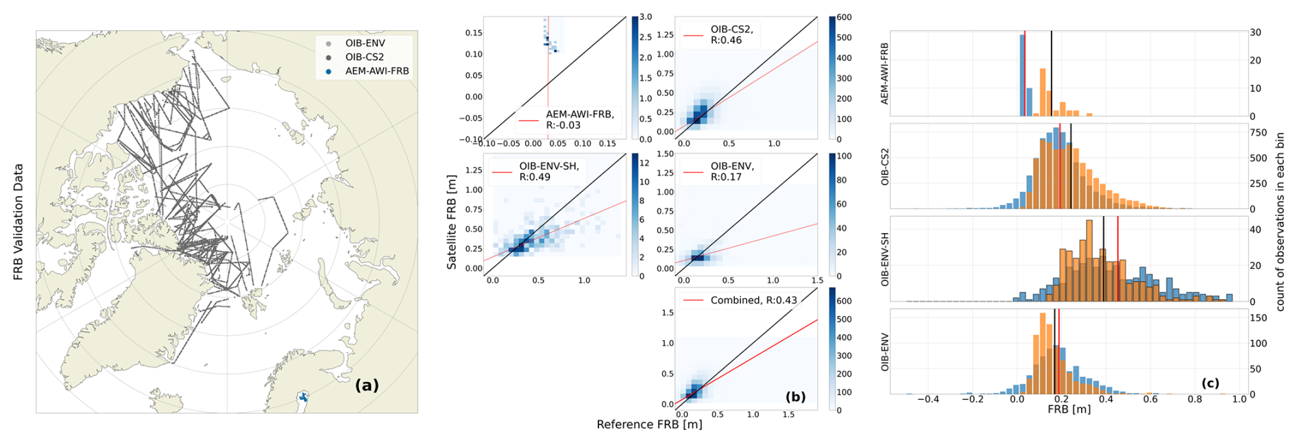
Figure 6FRB satellite and reference measurements comparison for CryoSat-2 (CS2) and Envisat (ENV) combined. The campaign names are followed by the satellite abbreviation, to highlight which satellite the reference measurements have been collocated to. (a) map of available overlap data for NH, (b) scatterplot with NH data with uncertainty weighted linear fits and associated correlation coefficients in the legend and (c) histograms with the reference measurements and satellite CDRs marked with blue and orange, respectively, with associated average as red and black vertical lines. A black outline around the histogram bins are added to data from the SH.
When examining Figs. 6–9, it is important to note that the main objective of this paper is not to conduct an inter-comparison study but rather to present the applications of the CCI SIT RRDP. Therefore, we focus on demonstrating how the database of reference measurements can be utilized to validate satellite products by highlighting the advantages and limitations of the different types of reference measurements. Furthermore, we discuss the availability of reference measurements for validating the four primary variables (FRB, SIT, SID and SD) for CryoSat-2, Envisat and ERS-1/2, respectively.
7.1 Freeboards (FRB)
The amount of reference measurements for freeboard validation included in the CCI SIT RRDP is limited to airborne campaign data, primarily collected in March and April in NH (Sect. 2.1, Fig. 5a). Nevertheless, airborne reference measurements show a good geographic representation in the western Arctic i.e., the Beaufort Sea, the Canadian Archipelago, as well as the Lincoln and Wandel Seas north of Greenland, and to a less degree the Fram Strait with CryoSat-2 and a reasonable overlap with Envisat (Fig. 6). However, no data are available for eastern Arctic including the East Siberian, Laptev, Kara and Barents Seas due to logistical challenges operating in these regions. For SH, FRB reference measurements are currently limited to OIB campaign data from October 2009 and 2010 (Sect. 2.1, Fig. 5b) collected in the Weddell, Bellingshausen and Amundsen Seas (Fig. 10a). Thus, no airborne FRB reference measurement data is available for CryoSat-2 in the SH in our CCI SIT RRDP. The associated histograms in Fig. 6c show similar distributions for NH OIB and CryoSat-2 FRB with −0.05 m mean difference (Table B1). Envisat is over-represented in thin sea ice thicknesses (FRB < 0.20 m NH) and has, in general, a narrower distribution compared to OIB FRB in NH, which is not reflected in the mean difference of 0.02 m (Table B2).
Reference measurements from AEM-AWI NH and OIB SH presents total FRB. Therefore, they are compared to the collocated satellite-derived sea ice FRB plus SD from the auxiliary snow depth information as provided in the CCI SIT CDR (Sect. 6.2) using Eq. (10). AEM-AWI FRB only includes data from the Baltic Sea, which is reflected in the low total FRB heights (< 0.3 m) representative for FYI. The limited geographical extent and the limited data amount of the AEM-AWI total FRB is expected to be one of the causes of the negative correlation coefficient (R= −0.03) as seen in Fig. 6b. Additionally, we do not know how well Envisat performs in the Baltic Sea, which is an area with only FYI and confined by land with many small Islands, which may impact the relatively large footprint size of Envisat. The over-representation of Envisat total FRB for thinner ice is also present in the SH when compared to OIB. The over-estimation of thin sea ice and a more narrow distribution is presumed to be a consequence of the different footprints of Envisat and CryoSat-2, and not caused by the reference measurements.
7.2 Thicknesses (SIT)
The amount of NH SIT reference measurements is more substantial than is the case for FRB and includes observations from airborne campaigns, ships, and ice mass balance buoys, which complement each other in terms of spatial and temporal coverage. For CryoSat-2 (Fig. 7a) reference measurements are well covered in the western Arctic region and also include some reference measurements in the eastern Arctic north of 80° N. However, most of the reference measurements in the eastern Arctic are based on visual ship observations. Reference measurements overlapping with Envisat are sparse and limited to few drifting buoys and airborne campaigns in the Beaufort Sea and the Fram Strait (Fig. 7d). SIT reference measurements to compare with ERS-1/2 are limited to some AEM-AWI airborne observations around Svalbard in the NH (Fig. 10b). In SH, SIT reference data is limited to visual ship observations from ASPeCt (Fig. 10a and c).
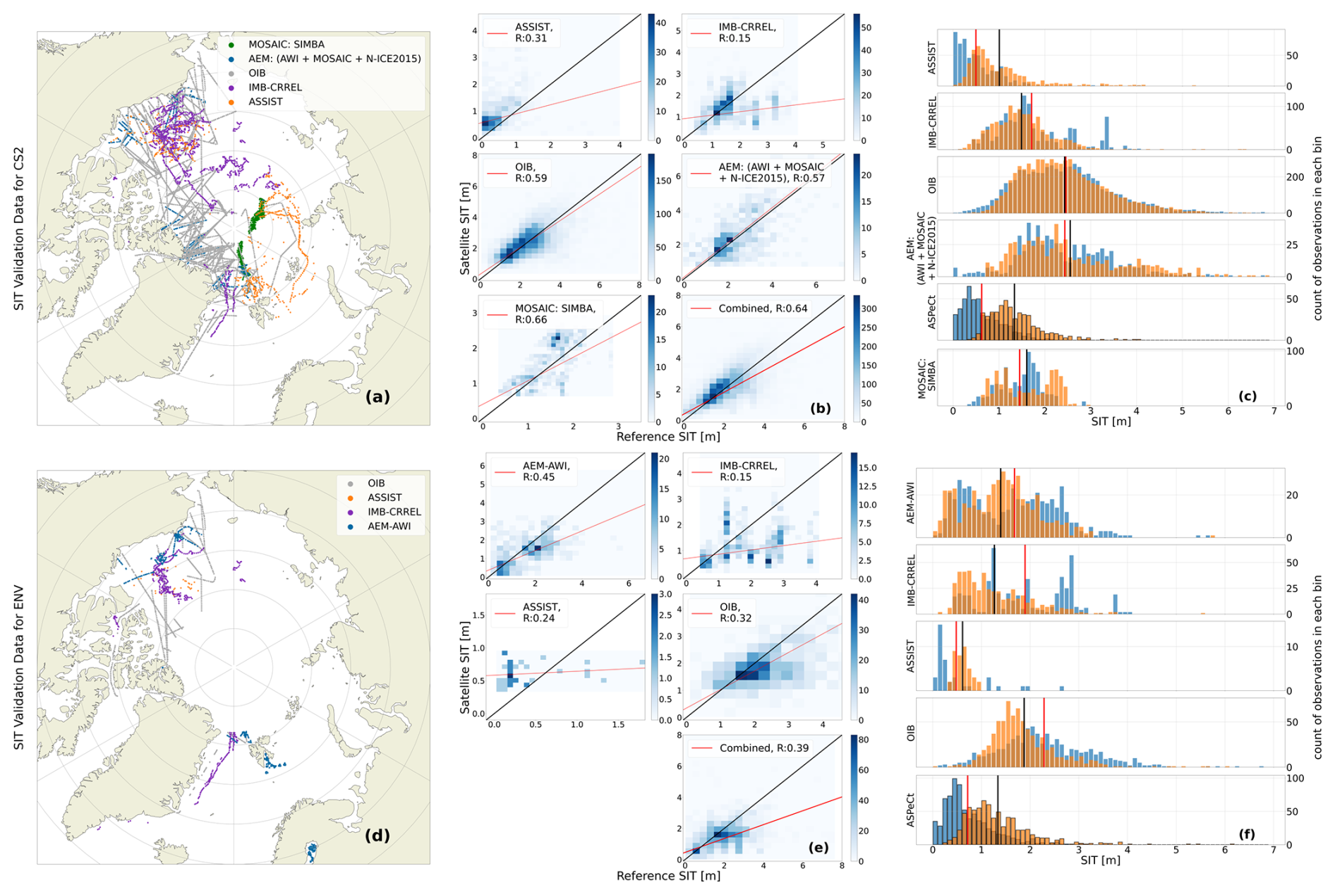
Figure 7SIT satellite and reference measurements comparison for CryoSat-2 (a–c) and Envisat (d–f). Maps of overlap data are shown for NH in (a) and (d), associated scatterplots with uncertainty weighted linear fits and associated correlation coefficients in the legend in (b) and (e) and histograms in (c) and (f). In the histograms the reference measurements and satellite CDRs are marked with blue and orange, respectively, with associated average as red and black vertical lines. A black outline around the histogram bins are added to data from the SH.
A reasonable overlap is found between the distribution of IMB and CryoSat-2 SIT (Fig. 7c) with a mean difference of 0.22 m, where IMB SIT is thicker than CryoSat-2 SIT. However, we did not find a linear relationship between the two datasets, as evidenced by the low correlation coefficient (Fig. 7b) and the R2≈0 value (Table B1). This is mainly expected to be due to the acquisition method, as mentioned in Sect. 4 resulting in a QFS of category 3 for buoys, as each buoy is measuring the temporal evolution of the same ice floe. Hereby, the measurements are local and do not capture variations in the surrounding ice as measured on satellite scales e.g, the growth of new ice and thicker ice, and deformation caused by the divergent and convergent motion of sea ice. As ice mass balance buoys must be placed on stable ice floes, this means they tend to be slightly biased toward thicker ice. This bias arises from the need to ensure that the ice floes do not melt or deform in ways that could damage the buoy or lead to its premature loss. In contrast, satellites measure a much larger area, which likely explains the weak linear relationship between the two. Contrary to IMB-CRREL buoys, MOSAiC SIMBA buoys have a high correlation (R=0.66), which is likely due to MOSAiC SIMBA buoys being a part of a distributed network. Nevertheless, as will be shown in Sect. 7.6 the low correlation between IMB-CRREL and CryoSat-2 and Envisat is strongly linked to the method of comparison. Alternative approaches, other than the one presented in Fig. 7, may be more suitable.
The use of the visual ship observations, as reference measurements for SIT, is dubious, as is also reflected in the assigned QFS of category 3 (see Sect. 4). First, visual ship observations contain a substantial degree of subjectivity, which introduces a larger uncertainty on the individual measurements in particular if the “IceWatch” manual (Hutchings et al., 2018) is not followed in detail and the observer is un-experienced. Additionally, as stated in U.S. Fleet (2007, Chap. 7), ships tend to choose the fastest and most economical route, which usually means avoiding ice to the highest degree possible by navigating in areas with thin ice, in leads or where there is low concentration. Additionally, Hutchings et al. (2018) states that only level ice should be recorded due to the likelihood of thicker ice not fully overturning. These factors combined suggests that observations from ships tend to have a larger representation of thin ice in the SIT distribution. Likewise the SD distribution also only represent conditions of level, easy-to-navigate sea ice.
This tendency is clearly reflected in the ASSIST and ASPeCt SIT distributions when compared both to CryoSat-2 and Envisat (Fig. 7c and f). This results in large negative biases of −0.51 and −0.71 m, when comparing ASSIST and ASPeCt SIT to CryoSat-2 SIT. Similar large negative bias of −0.62 m is found between ASPeCt and Envisat SIT, whereas the bias is smaller for ASSIST (−0.13 m). This is expected to be partly due to the limited amount of available ASSIST reference data overlapping with Envisat (Fig. 7d). As shown in Table B2 39 data points are available in the CCI SIT RRDP after averaging. In general, few ship observations are averaged for each value in the CCI SIT RRDP, as a result of limited data availability for each 25 km (50 km) grid cell for NH (SH). As a reference, on average 1.1 observations are used per average for the ASSIST measurements coinciding with Envisat and 1.95 for CryoSat-2. This means that the 39 available data points from ASSIST to Envisat represent a limited amount of information and are therefore associated with a larger uncertainty in their ability to represent the actual, larger-scale SIT and SD conditions.
In Sect. 7.6 and particularly in Fig. 11 an example of applying a filter of QFS <3 is presented, showing that the comparison between CryoSat-2 and SIT reference measurements can be vastly improved by excluding measurements from drifting buoys and ships.
7.3 Sea ice draft (SID)
SID data has a very limited geographical representation, as seen in Fig. 8a for CryoSat-2 and Fig. 8d for Envisat, and Fig. 10b for ERS-1/2 in NH, as most of SID data (except for SCICEX) are obtained from stationary moorings. However, the moorings represent a time-averaged SID and thus represent a larger sample of sea ice due to sea ice drift (Sect. 2.2), and have been used extensively to validate satellite-derived SIT (e.g. Sallila et al., 2019; Quartly et al., 2019). A reasonable agreement is seen in the distributions (Fig. 8c) between CryoSat-2 and SID data from SCICEX, NPI-FS, Nansen_legacy and BGEP.
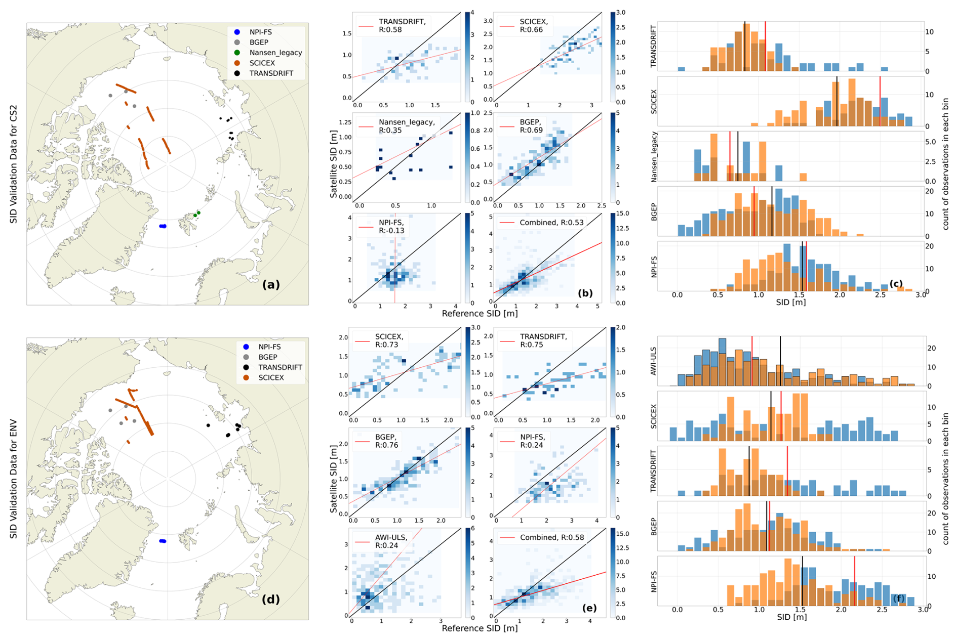
Figure 8SID satellite and reference measurements comparison for CryoSat-2 (a–c) and Envisat (d–f). Maps of overlap data are shown for NH in (a) and (d), associated scatterplots with uncertainty weighted linear fits and associated correlation coefficients in the legend in (b) and (e) and histograms in (c) and (f). In the histograms the reference measurements and satellite CDRs are marked with blue and orange, respectively, with associated average as red and black vertical lines. A black outline around the histogram bins are added to data from the SH.
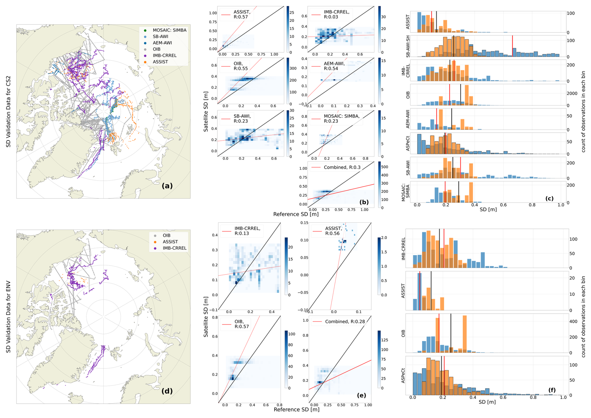
Figure 9SD satellite and reference measurements comparison for CryoSat-2 (a–c) and Envisat (d–f). Maps of overlap data are shown for NH in (a) and (d), associated scatter density plots with uncertainty weighted linear fits and associated correlation coefficients in the legend in (b) and (e) and histograms in (c) and (f). In the histograms the reference measurements and satellite CDRs are marked with blue and orange, respectively, with associated average as red and black vertical lines. A black outline around the histogram bins are added to data from the SH.
The TRANSDRIFT data are the only sea ice reference measurements available for the Seas north of Russia, and represent data over assumed fairly level FYI (the ideal sensing scenario for CryoSat-2). In Belter et al. (2020b) they find a correlation coefficient (R=0.47) and a mean difference (0.28 m) using orbit information from CryoSat-2 similar to our approach. These values are similar to those found in this study (R=0.58) and mean difference of (0.25 m). Their findings of a general tendency of satellite CDRs to overestimate SID < 0.7 m and underestimate SID > 1.3 m are in agreement with our findings. The SID distributions for Envisat and reference measurements in NH (Fig. 8f) are similar to those discussed for Envisat SIT in Sect. 7.2, where Envisat tends to be overrepresented in thinner ice and vise versa for thicker ice. This effect is most pronounced in comparison with SCICEX and TRANSDRIFT SID, where the reference measurements show SID values up to 3 m while Envisat SID remains below 1.8 m. Nevertheless, a good agreement is seen when comparing the Envisat and BGEP distributions, which is also reflected in the small mean difference of 0.03 m. Furthermore, high correlation coefficients are observed for all data except for NPI-FS and AWI-ULS, ranging between R=0.73 and R=0.76. SID data from NPEO is also available in the CCI SIT RRDP, but this data is located at the north pole and is, therefore, within the pole hole of the existing radar altimetry satellite missions. Nonetheless, the data has been included to validate satellite products or model data which have been interpolated across the pole hole. The strength of the SID reference measurement record is that NH NPI-FS and SCICEX covers both CryoSat-2, Envisat and ERS-1/2.
The representation of SID data for SH (Fig. 10a and c) is limited to moorings in the Weddell Sea and Lazarev Sea, which only overlaps with Envisat and ERS-1/2. This data shows a reasonable overlap in the distributions, although AWI-ULS tend to have more measurements of low SID (< 0.5 m, see Fig. 8f). AWI-ULS SID is on average 0.32 m lower when compared to Envisat SID if no bias correction is applied. Moreover, no significant trend (R2∼0) is seen between Envisat SID and AWI-ULS SID (Table B2).
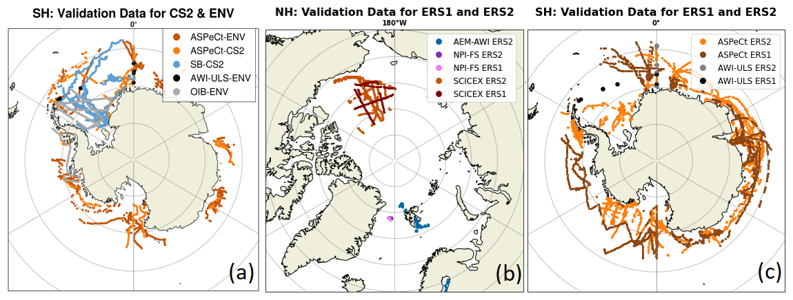
Figure 10Maps showing the geographical representation of; (a) SH reference measurements collocated with CryoSat-2 and Envisat data, (b) NH reference measurements collocated with ERS-1/2 and (c) SH reference measurements collocated with ERS-1/2.
7.4 Snow depth (SD)
A quite extensive amount of SD reference measurements are available for the NH in particular overlapping with CryoSat-2 (Fig. 9a), and to a lesser extent Envisat (Fig. 9d), including airborne, buoy and ship data. The geographic distribution of SD reference measurements is similar to the SIT (see Sect. 7.2). For SH, ASPeCt ship observations are available as presented in Fig. 10a for CryoSat-2 and Envisat, and in Fig. 10c for ERS-1/2. Snow depth measurements from buoys (SB-AWI-SH) are only available for CryoSat-2.
The comparison of the distributions presented in Fig. 9c and f shows large variability. The auxiliary snow depth products provided in the CCI SIT CDRs tend to exhibit narrower distributions compared to the various reference measurements. This suggests that these products supporting the satellite-derived sea ice thicknesses (described in Sect. 6.1), do not adequately capture the full variability of the snow depth distribution, particularly in the SH, where the auxiliary SD data used in the CCI SIT CDR are based on daily satellite radiometer observations. However, the variability may also be caused by the reference data having too high a variability, which may not signify the large scale variability of satellite products. This was also discussed in Stroeve et al. (2020) for drifting buoy observations of snow depths compared to models of similar spatial resolution (25 km) as for the CCI SIT CDRs in NH. Further work should be prioritized to improve this.
Nevertheless, reasonably high correlation coefficients (R>0.45, Fig. 9b and e) are obtained for several SD reference measurements such as ASSIST, AEM-AWI and OIB. Therefore, although the distributions do not show strong agreement, some degree of linear correlation is observed between the satellite SD product for some, but not all, sources of reference measurements.
7.5 Uncertainty quantification
Accurate uncertainty quantification is crucial to obtain the full potential of reference observations. However, this requires individual uncertainty measurements, that are ideally propagated all the way from the raw measurements through the processing chain to the final estimates. In this study, uncertainties have been assumed to be independent. However, this assumption is likely not valid and is expected to lead to an underestimation of the uncertainties in the CCI SIT RRDP. However, in lack of more accurate estimates, these values provide a first assessment of uncertainties and can be used as an alternative to the uncertainty values provided in Table 7. In the future, all reference measurements (buoy, airborne, submarine, and ship) should be quantified with individual uncertainty measurements or provided with uncertainty estimates that take into account some degree of seasonal/spatial variation.
An additional source of uncertainty in the CCI SIT RRDP arises from the representativeness of the reference data within a 25/50 km grid cell over a monthly period. To address this, we provided the standard deviations and the number of entries for each grid cell. However, differences in spatial and temporal coverage both between reference measurements and between satellite products within a 25/50 km grid cell over a monthly period may introduce temporal and spatial biases that are not captured in this analysis. Nevertheless, this study provides an initial assessment and takes steps toward a unified uncertainty estimate for SIT reference measurements. A comprehensive description will require future iterations and the inclusion of additional information. Further discussion of this topic is provided in Sect. 7.7.
7.6 Filtering and flagging
As described in Sect. 3.1, global filters have been applied in the CCI SIT RRDP, where all reference measurements with values below 0 have been replaced with NaN, and removed if SIT > 10 m, SID > 8 m, SD > 2 m or FRB > 2 m. Apart from these filters, the only additional filtering involved the removal of clearly erroneous data, such as the IMB-CRREL data from 2017 (see Sect. 5.2.3). As mentioned in Sect. 6.2, satellite observations and reference measurements have been gridded using the median and robust standard deviation, which makes the dataset less sensitive to outliers. Nevertheless, data in the CCI SIT RRDP include reference measurements with high robust standard deviations and/or that are based on only very few input measurements. If the standard deviation is high, the data may either contain outliers potentially caused by faulty measurements or reflect substantial variation in the reference measurements within the respective grid cell. This could indicate complex ice topography or conditions where sea ice (or snow) has undergone significant changes during the reference observation period (up to a month) within the grid cell, such as deformation or redistribution. On the other hand, a small number of reference measurements within a grid cell may suggest that the reference data are not representative of the entire area and/or time period.
Nevertheless, these considerations are closely related to the nature of the measurements and the applied methodology. For example, airborne campaigns often yield a high number of individual observations, but these are typically confined to a few days within a specific region. When such limited temporal and spatial coverages is compared with a monthly average from the CDR, questions arise regarding the representativeness of the comparison. A more detailed analysis of this issue is provided in Sect. 7.7.
To maximize the usability of the CCI SIT RRDP, quality flags are provided for the data (Sect. 4). The temporal quality flag (QFT) describes how temporally representative the data are, whereas the spatial quality flag (QFS) aims at describing how spatially representative the data are. An example of filtering of CryoSat-2 data using QFS < 3 is shown in Fig. 11. As seen, this removes all of the IMB and ASSIST data due to their known limitations in terms of spatial representativeness. For airborne data (AEM and OIB), this removes datapoints where the number of observations is below the 25 % quartile of the respective data source. For the remaining data, we observe a strong overlap in both distributions, with low median differences of 0.04 and −0.14 m, a relatively high combined correlation (R=0.59), and an ODR regression line close to the 1:1 line.
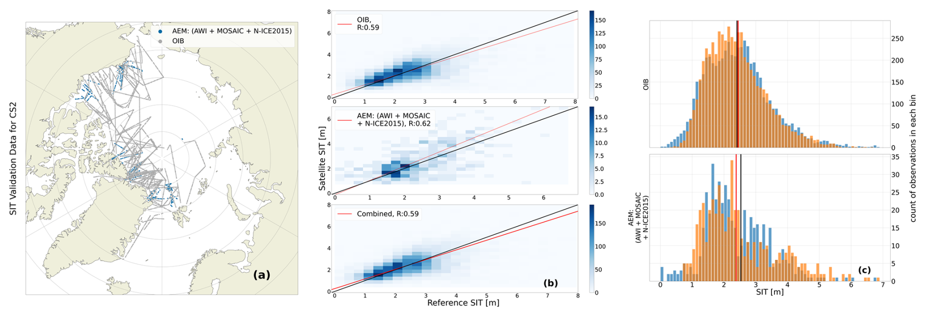
Figure 11Similar to Fig. 7 (a–c), but after applying the spatial representativeness quality flags (QFS < 3) to filter the reference measurements.
Other methods, such as matching the satellite SIT CDRs and reference measurements from drifting buoys and stations in a Lagrangian framework, i.e., following the buoy trajectories, might be a more suitable methodology for future comparisons. This approach was successfully demonstrated by Stroeve et al. (2020), who compared snow depths from the CRREL-IMBs and snow depth buoys to a snow depth model with spatial scales similar to the NH satellite products used in our study. As an alternative, inspired by previous studies (e.g., Guerreiro et al., 2016), the buoy data have also been compared as time series relative to the satellite CDR time series, rather than relying solely on absolute measurements. An example of this approach is presented in Fig. 12. Here, we observe that although issues related to spatial representativeness reduce the comparability between satellite and buoy observations, the overall accumulation during the data period is generally captured by both CryoSat-2 and the reference measurements. Moreover, comparability improves when filtering by the temporal flag (QFT). An example of filtering using the QFT is presented in Fig. 12b+d, where an overall increase in correlation is observed when applying high temporal representativeness filter (QFT ≤ 1). For MOSAiC SIMBA data, the correlation increases from 0.78 to 0.82 with a similar bias and RMSE for snow depth. In contrast, for the IMBs, the correlation changes from −0.47 to 0.15, while the bias decreases from 0.05 m to −0.03 m and RMSE from 0.24 to 0.09 m. Most strikingly for SD is the change of SB-AWI which increases from 0.46 to 0.61 in correlation and reduces by 0.05 m in bias and 0.04 m in RMSE, respectively. SIT estimates for MOSAiC SIMBA dataset show highly favorable statistics with a correlation coefficient of 0.94, which increases to 0.97 with QFT filter applied. The bias improves from −0.10 to −0.05 m, and the RMSE decreases from 0.26 to 0.16 m. We hypothesize that the favorable statistics of MOSAiC SIMBA relate to the fact that the MOSAiC SIMBA buoys were part of a distributed network, and therefore better represent the spatial conditions observable by the satellite. However, this aspect is currently not included in the spatial flag, which for the buoys, is based on the assumption that the conditions of only one floe are represented. An update to the flag could include identifying whether multiple buoys from different floes are present within a single grid cell and, similar to airborne data, computing the spatial extent covered by such buoys. An interesting change when applying the QFT flag is observed for IMB (Fig. 12c, d), where the correlation decreases from 0.81 to 0.56, the bias increases from −0.01 to −0.17 m, and RMSE increases by 0.15 m. Qualitatively, it shows that the winter of 2010/2011 for the IMB presents an opposite relationship (thinning of the ice during the winter season). Exploring it further, only 59 out of 183 (∼ 32 %) IMB observations are included for that winter period if QFT ≤ 1 is applied. The insets of Fig. 12c, d (point observations in red) show the buoy tracks from the 2010/2011 winter season and illustrate how the entire track through the Fram Strait (likely due to the high drift speeds) is discarded. The high thickness observations in the time series appear to be associated with the two buoys located in the fast ice region of the Canadian Archipelago, which skews the distribution and affects the monthly derived time series. One could filter by including information on basins (e.g., Central Arctic Ocean or Barents Sea as examples) to limit the potential impact that buoys deployed on landfast ice might introduce. We note that this sensitivity analysis was based on filtering with the flags prior to producing the monthly time series. However, this comparison appears more favorable than comparing with absolute observations, and allows for the inclusion of many reference measurements from across the basin to produce one estimate, which minimizes the impact of different type of representation within a grid cell between the two data sources.
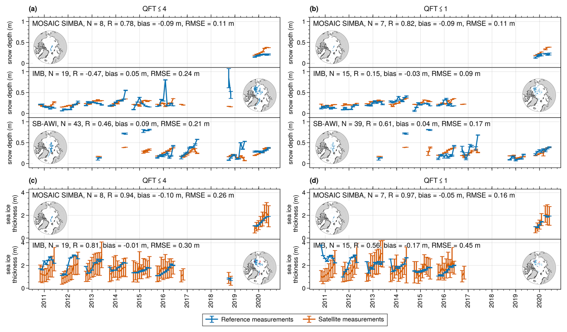
Figure 12Time series of reference measurements from IMB-CRREL, MOSAIC SIMBA and SB-AWI and CS2 satellite observations for collocated data. Each point represents the NH monthly average of all available buoys of a given type and the monthly average of collocated satellite observations, and with the example of utilising the temporal quality flag (QFT) applied (see Table 5 for a description of the flag). Error bars present the averaged standard deviation of the specified variable per grid cell included provided in the data product (see also Table 3 for the RRDP data set structure), bias is computed as the satellite measurements subtracted from the reference measurements, and RMSE is the root-mean-square-error. The inset shows the spatial extent of buoy observations included in the monthly time series (in blue), where in (c) and (d) for IMB, red denotes the observations from winter season 2010/2011 included in the time series (dependent on QFT) which is discussed in the text.
7.7 Representativeness and stability
Another important topic is the representativeness of the collocated satellite data when compared to the reference measurements. While the spatial and temporal filters help to some extent in quantifying representativeness issues, they are also restrictive and may lead to the removal of a significant portion of the reference measurements if applied too strictly. For instance, the combination of a QFS < 3 and a QFT < 3 for SIT would result in almost no reference data (8 observations ≈0.08 %), as the majority of airborne data would be removed by the temporal representativeness filter. This raises the question of whether using another collocation window for satellite measurements would be more appropriate for certain data types. To test this, we have made a representation error study using OIB data as the test case. We applied collocation windows varying in temporal sampling between 4, 16 and 30 d and in spatial sampling varying between 5, 15 and 25 km. The result of this analysis is shown in Fig. 13. For the comparison, we consider only the grid cells that contain collocated data across all collocation categories mentioned above. The analysis shows that decreasing the spatial radius of observations tends to reduce the correlation, whereas changing the temporal window has little effect.
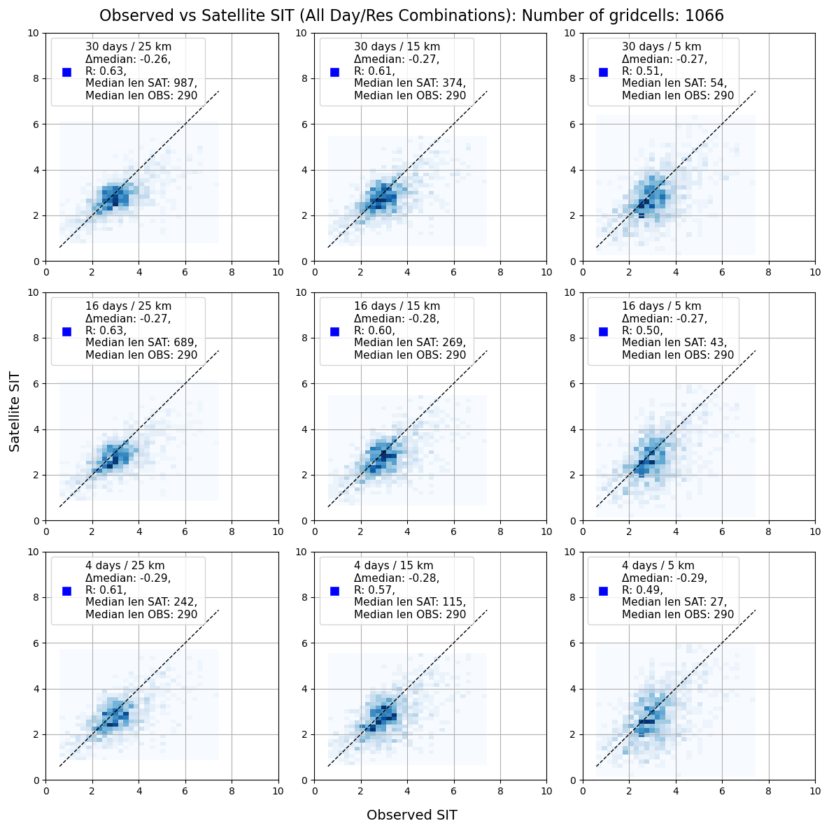
Figure 13Scatterplot of collocated OIB and CryoSat-2, when varying temporal sampling windows between 4, 16 and 30 d and spatial sampling windows between 5, 15 and 25 km. Only gridcells that appear when applying the smallest spatial and temporal windows (4 d and 5 km) are included.
To understand these results, we refer to Fig. 14. This figure shows one OIB track (green) along with available satellite orbit tracks within a 25 km radius and a ±15 d temporal window. It illustrates that the OIB flight track follows one of the satellite orbit tracks, but for this case not the one closest in time (may not have been the target track of the flight campaign). If a small temporal window is chosen, this track would therefore not be included in the comparison. Similarly, a smaller spatial window will result in the inclusion of satellite measurements that only cover parts of the OIB track. Overall, it also showcases the effect of comparing monthly gridded satellite data, which can cover a grid cell more comprehensively than a one-day OIB track. Furthermore, the footprint sizes illustrate the varying information available from each data source, even if they were to fly along the same track. Such issues are inherent to the data itself as the resolution differs, and future work should investigate how to further minimize the impact of these scaling issue between data sources (see also Xu et al., 2020).
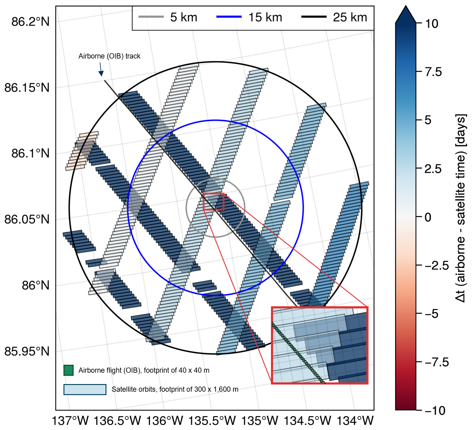
Figure 14Example of spatial representativeness for one grid cell of the EASE2 grid (with center location at 87.38° N and −154.68° E) with an airborne track (OIB-QL) flown on 22 April 2019 and satellite tracks (CryoSat-2) within the vicinity in time (using a temporal span of maximum ±15 d) and space (using search radii of 5, 15, and 25 km denoted by the circles). Footprints of the different sources are visualised using 40 × 40 m for OIB-QL and 1600 × 300 m for CryoSat-2. Δt describes the temporal difference between the airborne and satellite measurements in days.
To test the stability of the satellite-based SIT CDRs with reference measurements, we here recommend using a combination of the long-term monitoring programs, i.e., upward-looking moorings from the Beaufort Gyre Exploitation Project (BGEP), the Fram Strait Arctic Outflow Observatory (NPI-FS) and the Russian-German TRANSDRIFT project (TRANSDRIFT), together with submarine cruises (SCICEX) and airborne EM-campaigns (AEM-AWI) for NH. A similar extensive dataset is not available for the SH because the AWI-ULS only cover the Envisat period and ASPeCt SIT and SD reference measurements are biased towards the thinner end of the SIT and SD distributions. To combine the NH measurements into a trend dataset, we need to align the reference measurements and the satellite SIT CDRs to a common measurand, e.g., total SIT or draft. For consistency, one must ensure that a common baseline for auxiliary information of SD and densities of sea ice, snow and water is used. Thus, we encourage the community to include the information on all auxiliary data used to support the radar-freeboard-to-sea-ice-freeboard and sea-ice-freeboard-to-thickness conversions in their datasets. Furthermore, we note that the reference measurements included in the CCI SIT RRDP have been prepared in a format consistent with satellite products (here primarily the CCI SIT CDRs), which are provided as monthly, gridded datasets. However, efforts should also be made to investigate how to utilise other available datasets to validate the lower level (e.g., Level-2) satellite observations, and contribute to the discussion of the formats which reference measurements should be collected to ensure that satellite observations can be deemed fit for purpose and fulfilling of their mission requirements.
The CCI SIT RRDP dataset is available at DTU DATA (https://doi.org/10.11583/DTU.24787341) (Olsen and Skourup, 2026a) and released under a CC-BY 4.0 license. The final data files are formatted as NetCDF files with not-a-number (NaN) denoting missing data. Apart from the final dataset, all the source code used in the processing steps from the original reference observations to the final CCI SIT RRDP, together with procedures for collocating the CCI SIT RRDP to the satellite measurements from CryoSat-2, Envisat and ERS-1/2, and for creating Figs. 3–12 and 14 are available on Zenodo (https://doi.org/10.5281/zenodo.14808968) through Olsen and Skourup (2026b). By providing links to the original reference measurements and satellite data (Table 2), this ensures transparency and equips users with the tools and data needed to fully reproduce the final data set. It also allows users to easily redefine their own temporal and spatial scales tailored to their specific needs. In the ReadMe file in GitHub (Olsen and Skourup, 2026b) is specified how the temporal and spatial resolutions can be adjusted in the provided scripts. Figure 2 (Sankey diagram) was produced using the online tool “VisualParadigmOnline”, and adapted in Microsoft Office Power Point. Figure 14 has been developed from adapted scripts of Fredensborg Hansen (2024) using intermediate data developed within the framework of the RRDP, which is not provided in the final output version of the data product, and the script to produce this figure is therefore not provided publicly.
Here, we have presented the CCI SIT RRDP (Olsen and Skourup, 2026a), which is a collection of publicly available non-satellite sea ice thickness observations covering the polar satellite era 1993–2024 including freeboards (total, radar or derived sea ice), thicknesses (total or sea ice), drafts and snow depths from different sources. We have prepared the CCI SIT RRDP to be suitable for comparison of satellite altimeter observations of sea ice freeboard, sea ice thickness and auxiliary snow depth products, but it can also be used for comparison of e.g. models. The observations have been prepared to a level where they can be directly compared to satellite altimetry temporal (monthly) and spatial (25 km NH; 50 km SH) scales, but these can easily be changed by using the CCI SIT RRDP software package Olsen and Skourup (2026b). We have added uncertainties to the associated reference measurements and flagged these according to their reliability, as well as flagged data according to spatial and temporal representativeness, caused by the inherent nature of the various measurements.
As examples of how this data package can be used, we have compared them with the CCI SIT CDRs from CryoSat-2 and Envisat. Here, we generally find good agreement across the different reference measurements included in the CCI SIT RRDP. Visual observations of sea ice thickness and snow depths from ship cruises cannot be used as reference measurements for satellite altimetry in the present form presented in the RRDP, as they are biased low in their distributions. This is expected as ships tend to navigate through the thinnest ice. Furthermore, care should be taken when using OIB QL products due to existing biases in snow depth processing, as this dataset were only meant to be processed for a quick assessment of the data and not designed as a long- term archived dataset for satellite inter-comparison. In addition, the approach used in this study by gridding and time-averaging observations from drifting buoys to match satellite scales might not be the most optimal. Other methods, such as matching the satellite SIT CDRs and observations from drifting buoys in a Lagrangian framework might present a more suitable solution.
However, existing reference measurements are still scarce in the polar regions, even more pronounced in the Antarctic than in the Arctic. It is therefore necessary to include and use as much data as possible, while acknowledging the advantages and limitations of each method. We also note that data prior to 2011 is limited to a few reference measurements – even more so if we remove measurements carried out within the so-called pole hole, the area poleward of, e.g., 81.5° N for ERS-1/2 and Envisat – thus, limiting the comparisons to be made with these satellites. Existing potential reference measurements, which are not included in the CCI SIT RRDP, need to be made publicly available and processed to a level where they can directly be used for inter-comparison to satellite altimetry-derived observations before inclusion into the CCI SIT RRDP. This includes e.g., freeboards from ESA's CryoSat Validation Experiment (CryoVEx) campaigns, Antarctic total freeboards and snow depths from OIB campaigns after 2010. When satellite altimetry-derived sea ice thicknesses are provided in a CDR it is important for comparison and evaluation purposes to include all the auxiliary information used in the intermediate steps in the radar freeboard to sea ice thickness conversion.
For future work, it will be crucial to ensure that reference measurements follow the protocols and procedures for FRMs i.e., that they are traceable, and fully described with uncertainty diagrams, effects tables and comparability diagrams, see first efforts for altimetry derived sea ice thicknesses in Da Silva et al. (2023). Such comparability diagrams will also aid the design of campaigns to produce reference measurements which are directly comparable to satellite SIT products. As an example, the AWI IceBird Winter campaigns since 2017 use a sensor combination of EM-Bird, airborne laser scanner and snow radar that allows for a direct retrieval of sea ice thickness, sea ice freeboard and snow depth simultaneously (Jutila et al., 2022a). Updating the data package will be ongoing work to ensure it remains current and comprehensive. The community also urgently needs to ensure a consistent network of polar observations for continuous reference measurements of current and future satellite altimeter missions such as Copernicus Polar Ice and Snow Topography Altimeter (CRISTAL) (Kern et al., 2020). There are currently no concrete plans for updating the CCI SIT RRDP beyond 2026, where the project ends. However, we will seek other opportunities for a continuation within frameworks of related databases and projects e.g., St3TART-FO project (https://frm-datahub.noveltis.fr/, last access: 12 January 2026), SIN'XS (https://sinxs.noveltis.fr/, last access: 12 January 2026) or C3S (https://cis2.eea.europa.eu/about, last access: 12 January 2026). Otherwise, the code is readily available, making it easy for users to process and update the database with extensions or additional reference measurements.
| Abbreviation | Definition |
| AEM | Airborne Electromagnetic (measurements) |
| ATM | Airborne Topographic Mapper |
| CCI | Climate Change Initiative |
| CDR | Climate Data Record |
| CRISTAL | Copernicus Polar Ice and Snow Topography Altimeter |
| CryoVEx | CryoSat Validation Experiment |
| EASE2 | Equal-Area Scalable Earth grid, version 2 |
| ECV | Essential Climate Variable |
| EM | Electromagnetic |
| Envisat | Environmental Satellite |
| ERS-1/2 | European Remote Sensing Satellites 1 and 2 |
| ESA | European Space Agency |
| FDR4ALT | Fundamental Data Records for Altimetry |
| FRB | Freeboard |
| FRM | Fiducial Reference Measurements |
| GNSS | Global Navigation Satellite System |
| HEM | Helicopter Borne Electromagnetic |
| (measurements) | |
| ICESat | Ice, Cloud and land Elevation Satellite |
| LiDAR | Light Detection and Ranging |
| NASA | National Aeronautics and Space |
| Administration | |
| NH | Northern Hemisphere |
| NSIDC | National Snow and Ice Data Center |
| RA | Radar Altimeter |
| RRDP | Round Robin Data Package |
| SAR | Synthetic Aperture Radar |
| SH | Southern Hemisphere |
| SD | Snow Depth |
| SID | Sea Ice Draft |
| SIRAL | SAR interferometric radar altimeter |
| SIT | Sea Ice Thickness |
| ULS | Upward Looking Sonar |
| WGS | World Geodetic System |
The following tables show statistics related to the comparison of CCI SIT RRDP with Envisat CDR and CryoSat-2 CDR. The comparison includes the standard deviation (std) and average of the reference and satellite data, respectively. The root mean square error (RMSE), Pearson's correlation coefficient (R) (only shown in Figs. 6–9) and the coefficient of determination (R2) for both the best fit and the fit y=x, as would be the ideal case.
Due to the nature of R2 being a calculation between a true value and a fit, this calculation is highly sensitive to which variable is examined. In the case presented below the (R2) value is calculated between the satellite CDRs and the predictions.
Table B1Statistics of results CryoSat-2, LS = Least Squares, ODR = Orthogonal Distance Regression.
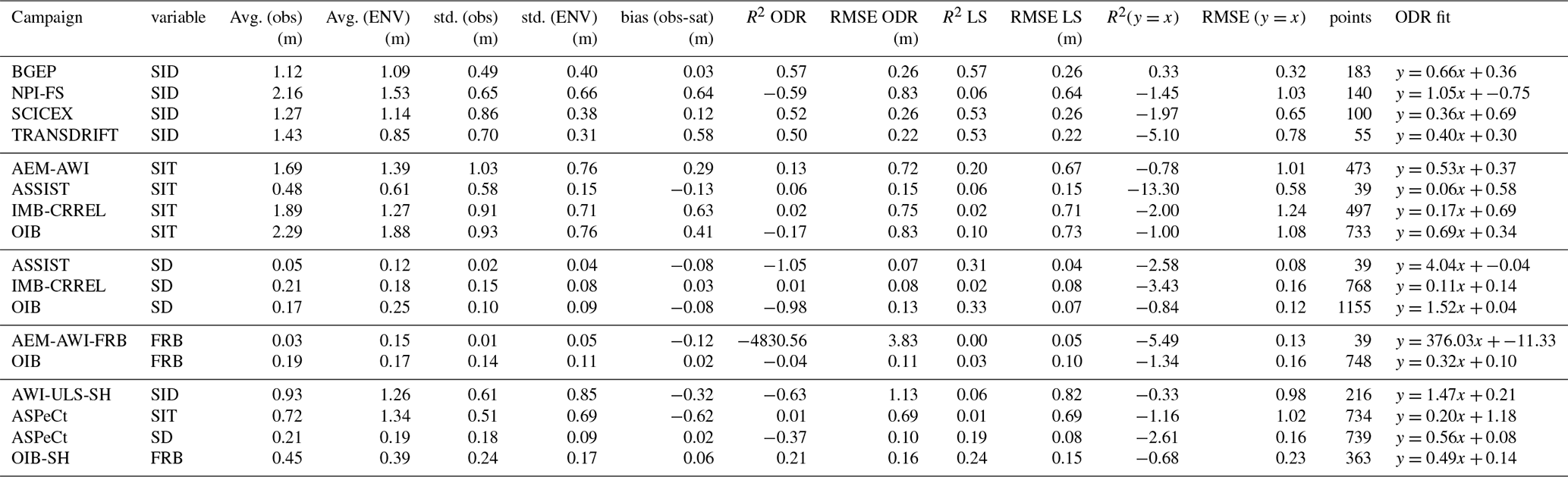
Table B2Statistics of results Envisat, LS = Least Squares, ODR = Orthogonal Distance Regression.
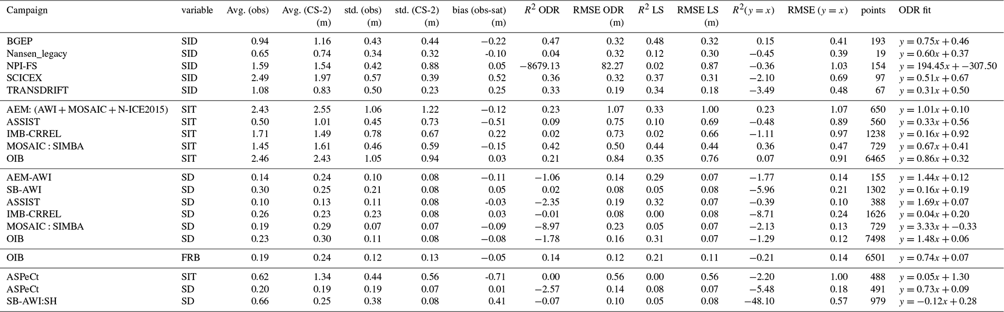
IO has collected and prepared the CCI SIT RRDP presented in this paper, including pre-processing, estimation of uncertainties and flags. The CCI SIT RRDP is based on previous versions prepared by HSK within the initial phases of the CCI SI project. The initial versions included only sea ice freeboards and snow depth, with no uncertainties or flags provided, https://ftp.spacecenter.dk/pub/SICCI/ (last access: 12 January 2026). IO further collocated the reference data with the satellite CDRs. IO, HSK, HS, RMFH wrote the initial manuscript, produced the figures, and specified the extended flagging procedure currently implemented. HSK, ER, SH, RMFH, and SK contributed by identifying relevant reference measurements and defining the temporal and spatial resolution together with the collocation procedures and initial uncertainty flagging procedures. They also contributed through discussions. HSK, ER, SK contributed to the development of the first phases of the CCI SIT RRDP, including validation. SH, SP, ER and HS contributed to satellite-derived CCI SIT CDRs from CryoSat-2 and Envisat. MB and SF contributed with ERS-1/2 data from the FDR4ALT project. DD contributed with NPI-FS mooring data. All authors contributed to the revision of the manuscript, which was led by IO and HSK, together with RMFH.
The contact author has declared that none of the authors has any competing interests.
Publisher's note: Copernicus Publications remains neutral with regard to jurisdictional claims made in the text, published maps, institutional affiliations, or any other geographical representation in this paper. The authors bear the ultimate responsibility for providing appropriate place names. Views expressed in the text are those of the authors and do not necessarily reflect the views of the publisher.
The main contribution to this work was conducted while IO was affiliated with DTU Space. The project and its results are primarily associated with this institution. IO is now affiliated with DMI, which contributed to the revision process of the manuscript. We thank DMI for their support during this phase.
We also express our sincere gratitude to everyone involved in the collection, preparation, maintenance and publication of the input data used in this study. These include, but are not limited to, the Beaufort Gyre Exploration Program based at the Woods Hole Oceanographic Institution (https://www2.whoi.edu/site/beaufortgyre/, last access: 12 January 2026) in collaboration with researchers from Fisheries and Oceans Canada at the Institute of Ocean Sciences, the Norwegian Polar Institute, the North Pole Environmental Observatory and the Polar Science Center, the Russian-German BMBF-funded TRANSDRIFT project, the Alfred Wegener Institute, the Norwegian Meteorological Institute, the Cold Regions Research and Engineering Laboratory, the SCAR Antarctic Sea Ice Processes and Climate (ASPeCt) program (https://aspect.antarctica.gov.au, last access: 12 January 2026), the U.S. Navy and Royal Submarines, and the Submarine Arctic Science Program, The Nansen Legacy research project, the Multidisciplinary drifting Observatory for the Study of Arctic Climate (MOSAiC) expedition and the Norwegian young sea ICE cruise (N-ICE2015). We acknowledge that it would not have been possible to create the Climate Change Initiative Sea Ice Thickness Round Robin Data Package without the up-to-date and publicly available reference data from the above sources.
We acknowledge the use of AI-based language tools (co-pilot and chatgpt) to assist in checking the manuscript for consistency and clarity. These tools were used to support language refinement without altering the scientific content.
We also acknowledge the important contributions of the CCI Sea Ice scientific leader, Thomas Lavergne, and project coordinator, Mari Anne Killie, both from the Norwegian Meteorological Institute (METNO). Their exceptional leadership, management, and insightful discussions have been pivotal to the success of this study.
Finally, we express our sincere appreciation to the reviewers for their thoughtful and constructive evaluations. Their insightful comments and suggestions have been invaluable in improving the clarity and overall quality of the manuscript.
This research has been supported by the European Space Agency (Climate Change Initiative (CCI) for sea ice (grant no. 4000126449/19/I-NB)).
This paper was edited by Clare Eayrs and reviewed by Alek Petty and one anonymous referee.
Andersen, O. B., Rose, S. K., Abulaitijiang, A., Zhang, S., and Fleury, S.: The DTU21 global mean sea surface and first evaluation, Earth System Science Data, 15, 4065–4075, https://doi.org/10.5194/essd-15-4065-2023, 2023. a
Arndt, S., Maaß, N., Rossmann, L., and Nicolaus, M.: From snow accumulation to snow depth distributions by quantifying meteoric ice fractions in the Weddell Sea, The Cryosphere, 18, 2001–2015, https://doi.org/10.5194/tc-18-2001-2024, 2024. a, b, c
ASSIST: Ice Watch ASSIST Data Network, Norwegian Metrological Institute [data set], https://cryo.met.no/en/icewatch (last access: 1 May 2025), 2006. a
Behrendt, A., Dierking, W., Fahrbach, E., and Witte, H.: Sea ice draft in the Weddell Sea, measured by upward looking sonars, Earth System Science Data, 5, 209–226, https://doi.org/10.5194/essd-5-209-2013, 2013a. a, b, c, d, e
Behrendt, A., Dierking, W., Fahrbach, E., and Witte, H.: Sea ice draft measured by upward looking sonars in the Weddell Sea (Antarctica) [dataset publication series], PANGAEA [data set], https://doi.org/10.1594/PANGAEA.785565, 2013b. a
Bell, S.: Measurement Good Practice Guide, A Beginner's Guide to Uncertainty of Measurement, Esscolab, 11, https://www.esscolab.com/uploads/files/measurement-guide.pdf (last access: 28 July 2023), 1999. a, b
Belter, H. J., Janout, M. A., Krumpen, T., Ross, E., Hölemann, J. A., Timokhov, L., Novikhin, A., Kassens, H., Wyatt, G., Rousseau, S., and Sadowy, D.: Daily mean sea ice draft from moored Upward-Looking Sonars in the Laptev Sea between 2013 and 2015, PANGAEA [data set], https://doi.org/10.1594/PANGAEA.899275, 2019. a
Belter, H. J., Janout, M. A., Hölemann, J. A., and Krumpen, T.: Daily mean sea ice draft from moored upward-looking Acoustic Doppler Current Profilers (ADCPs) in the Laptev Sea from 2003 to 2016, PANGAEA [data set], https://doi.org/10.1594/PANGAEA.912927, 2020a. a
Belter, H. J., Krumpen, T., Hendricks, S., Hoelemann, J., Janout, M. A., Ricker, R., and Haas, C.: Satellite-based sea ice thickness changes in the Laptev Sea from 2002 to 2017: comparison to mooring observations, The Cryosphere, 14, 2189–2203, https://doi.org/10.5194/tc-14-2189-2020, 2020b. a, b, c
Belter, H. J., Krumpen, T., Janout, M. A., Ross, E., and Haas, C.: An Adaptive Approach to Derive Sea Ice Draft from Upward-Looking Acoustic Doppler Current Profilers (ADCPs), Validated by Upward-Looking Sonar (ULS) Data, Remote Sensing, 13, https://doi.org/10.3390/rs13214335, 2021. a, b
BGEP: The data were collected and made available by the Beaufort Gyre Exploration Program based at the Woods Hole Oceanographic Institution in collaboration with researchers from Fisheries and Oceans Canada at the Institute of Ocean Sciences, https://www2.whoi.edu/site/beaufortgyre/data/mooring-data/ (last access: 1 May 2025), 2003. a, b
Bocquet, M. and Fleury, S.: Arctic and Antarctic sea ice thickness climate data record (ERS-1, ERS-2, Envisat, CryoSat-2), CTOH [data set], https://doi.org/10.6096/ctoh_sit_2023_01, 2023. a
Bocquet, M., Fleury, S., Piras, F., Rinne, E., Sallila, H., Garnier, F., and Rémy, F.: Arctic sea ice radar freeboard retrieval from the European Remote-Sensing Satellite (ERS-2) using altimetry: toward sea ice thickness observation from 1995 to 2021, The Cryosphere, 17, 3013–3039, https://doi.org/10.5194/tc-17-3013-2023, 2023. a, b, c
Bocquet, M., Fleury, S., Rémy, F., and Piras, F.: Arctic and Antarctic Sea Ice Thickness and Volume Changes From Observations Between 1994 and 2023, Journal of Geophysical Research: Oceans, 129, e2023JC020848, https://doi.org/10.1029/2023JC020848, 2024. a
Boggs, P. T. and Rogers, J. E.: Orthogonal Distance Regression, in: Statistical analysis of measurement error models and applications: proceedings of the AMS-IMS-SIAM Joint Summer Research Conference, 10–16 June 1989, Contemporary Mathematics, 112, 186, https://www.mechanicalkern.com/static/odr_ams.pdf (last access: 15 January 2026), 1990. a
Brodzik, M., Billingsley, B., Haran, T., Raup, B., and Savoie, M.: EASE-Grid 2.0: Incremental but Significant Improvements for Earth-Gridded Data Sets, International Journal of Geo-Information, 1, 32–45, https://doi.org/10.3390/ijgi1010032, 2012. a
Carret, A., Fleury, S., Di Bella, A., Landy, J., Lawrence, I., Kurtz, N., Laforge, A., Bouffard, J., and Parrinello, T.: A multi-frequency altimetry snow depth product over Arctic sea ice, Scientific Data, 12, https://doi.org/10.1038/s41597-024-04343-4, 2025. a
Cavalieri, D. J., Markus, T., and Comiso, J. C.: AMSR-E/Aqua Daily L3 12.5 km Brightness Temperature, Sea Ice Concentration, & Snow Depth Polar Grids, Version 3, NSDIC [data set], https://doi.org/10.5067/AMSR-E/AE_SI12.003, 2014. a
Cheng, Y., Cheng, B., Zheng, F., Vihma, T., Kontu, A., Yang, Q., and Liao, Z.: Air/snow, snow/ice and ice/water interfaces detection from high-resolution vertical temperature profiles measured by ice mass-balance buoys on an Arctic lake, Annals of Glaciology, 61, 309–319, https://doi.org/10.1017/aog.2020.51, 2020. a
Cristea, A., Gerland, S., and Bratrein, M.: Results of regional scale sea ice and snow thickness surveys during Nansen Legacy/Synoptic Arctic Survey Joint Cruise 2 (JC2-2) in August–September 2021 using helicopter-borne electromagnetic induction sounding instrument (EM-bird), Norwegian Polar Institute [data set], https://doi.org/10.21334/NPOLAR.2023.C1CFD5DD, 2023. a
Da Silva, E., Woolliams, E. R., Picot, N., Poisson, J.-C., Skourup, H., Moholdt, G., Fleury, S., Behnia, S., Favier, V., Arnaud, L., Aublanc, J., Fouqueau, V., Taburet, N., Renou, J., Yesou, H., Tarpanelli, A., Camici, S., Fredensborg Hansen, R. M., Nielsen, K., Vivier, F., Boy, F., Fjørtoft, R., Cancet, M., Ferrari, R., Picard, G., Tourian, M. J., Sneeuw, N., Munesa, E., Calzas, M., Paris, A., Le Meur, E., Rabatel, A., Valladeau, G., Bonnefond, P., Labroue, S., Andersen, O., El Hajj, M., Catapano, F., and Féménias, P.: Towards Operational Fiducial Reference Measurement (FRM) Data for the Calibration and Validation of the Sentinel-3 Surface Topography Mission over Inland Waters, Sea Ice, and Land Ice, Remote Sensing, 15, https://doi.org/10.3390/rs15194826, 2023. a, b, c
Divine, D., Bratrein, M., Jacobsen, J. A., and Gerland, S.: Results of regional scale sea ice and snow thickness surveys during Nansen Legacy Q1 research cruise in March 2021 using helicopter-borne electromagnetic induction sounding instrument (EM-bird), Norwegian Polar Institute [data set], https://doi.org/10.21334/NPOLAR.2023.1A9CC2DF, 2023. a
Fons, S., Kurtz, N., and Bagnardi, M.: A decade-plus of Antarctic sea ice thickness and volume estimates from CryoSat-2 using a physical model and waveform fitting, The Cryosphere, 17, 2487–2508, https://doi.org/10.5194/tc-17-2487-2023, 2023. a, b
Fredensborg Hansen, R. M.: cryo2iceant22-airborne-cryo2ice-weddell-sea-ice, Zenodo [code], https://doi.org/10.5281/zenodo.13749342, 2024. a
Giles, K. A. and Hvidegaard, S. M.: Comparison of space borne radar altimetry and airborne laser altimetry over sea ice in the Fram Strait, International Journal of Remote Sensing, 27, 3105–3113, https://doi.org/10.1080/01431160600563273, 2006. a
Grosfeld, K., Treffeisen, R., Asseng, J., Bartsch, A., Bräuer, B., Fritzsch, B., Gerdes, R., Hendricks, S., Hiller, W., Heygster, G., Krumpen, T., Lemke, P., Melsheimer, C., Nicolaus, M., Ricker, R., and Weigelt, M.: Online Sea-Ice Knowledge and Data Platform <https://www.meereisportal.de>, Alfred Wegener Institute for Polar and Marine Research & German Society of Polar Research [data set], https://doi.org/10.2312/polfor.2016.011, 2016. a
Guerreiro, K., Fleury, S., Zakharova, E., Rémy, F., and Kouraev, A.: Potential for estimation of snow depth on Arctic sea ice from CryoSat-2 and SARAL/AltiKa missions, Remote Sensing of Environment, 186, 339–349, https://doi.org/10.1016/j.rse.2016.07.013, 2016. a
Guerreiro, K., Fleury, S., Zakharova, E., Kouraev, A., Rémy, F., and Maisongrande, P.: Comparison of CryoSat-2 and ENVISAT radar freeboard over Arctic sea ice: toward an improved Envisat freeboard retrieval, The Cryosphere, 11, 2059–2073, https://doi.org/10.5194/tc-11-2059-2017, 2017. a
Haas, C.: Sea Ice, third edition, Chapter 2: sea ice thickness distribution, Wiley Blackwell, https://doi.org/10.1002/9781118778371, 2016. a
Haas, C., Göbell, S., Hendricks, S., Martin, T., Pfaffhuber, A., and Saldern, C.: Airborne electromagnetic measurements of sea ice thickness: methods and applications, European Commission, https://epic.awi.de/id/eprint/16589/1/Haa2007c.pdf (last access: 15 January 2026), 2007. a, b, c, d, e, f, g
Haas, C., Lobach, J., Hendricks, S., Rabenstein, L., and Pfaffling, A.: Helicopter-borne measurements of sea ice thickness, using a small and lightweight, digital EM system, Journal of Applied Geophysics, 67, 234–241, https://doi.org/10.1016/j.jappgeo.2008.05.005, 2009. a, b
Hendricks, S., Paul, S., and Rinne, E.: ESA Sea Ice Climate Change Initiative (Sea_Ice_cci): Northern hemisphere sea ice thickness from CryoSat-2 on the satellite swath (L2P), v3.0, CEDA Archive [data set], https://catalogue.ceda.ac.uk/uuid/c6504378f78c4ecd9f839b0434023eff (last access: 9 August 2024), 2024a. a, b, c
Hendricks, S., Paul, S., and Rinne, E.: ESA Sea Ice Climate Change Initiative (Sea_Ice_cci): Northern hemisphere sea ice thickness from Envisat on the satellite swath (L2P), v3.0, CEDA Archive [data set], https://catalogue.ceda.ac.uk/uuid/92eb2ba942074bec804af6a8b5436bee (last access: 9 August 2024), 2024b. a, b
Hendricks, S., Paul, S., and Rinne, E.: ESA Sea Ice Climate Change Initiative (Sea_Ice_cci): Southern hemisphere sea ice thickness from CryoSat-2 on the satellite swath (L2P), v3.0, CEDA Archive [data set], https://catalogue.ceda.ac.uk/uuid/861ad3c7f3a34ebd8be6f618a92bd8e3 (last access: 9 August 2024), 2024c. a, b, c
Hendricks, S., Paul, S., and Rinne, E.: ESA Sea Ice Climate Change Initiative (Sea_Ice_cci): Southern hemisphere sea ice thickness from Envisat on the satellite swath (L2P), v3.0, CEDA Archive [data set], https://catalogue.ceda.ac.uk/uuid/af96a1ec493f49caa39dc912d15f2b17 (last access: 9 August 2024), 2024d. a, b
Hutchings, J., Delamere, J., and Heil, P.: The Ice Watch Manual, Universität Hamburg, https://fiona.uni-hamburg.de/bdc0b40b/hutchings-ice-watch-manual-v4-1.pdf (last access: 9 February 2026), 2018. a, b, c, d, e, f
Jutila, A., Hendricks, S., Ricker, R., von Albedyll, L., Krumpen, T., and Haas, C.: Retrieval and parameterisation of sea-ice bulk density from airborne multi-sensor measurements, The Cryosphere, 16, 259–275, https://doi.org/10.5194/tc-16-259-2022, 2022a. a, b
Jutila, A., King, J., Paden, J., Ricker, R., Hendricks, S., Polashenski, C., Helm, V., Binder, T., and Haas, C.: High-Resolution Snow Depth on Arctic Sea Ice From Low-Altitude Airborne Microwave Radar Data, IEEE Transactions on Geoscience and Remote Sensing, 60, 1–16, https://doi.org/10.1109/TGRS.2021.3063756, 2022b. a, b, c
Jutila, A., Hendricks, S., Ricker, R., von Albedyll, L., and Haas, C.: Airborne sea ice parameters during the PAMARCMIP2017 campaign in the Arctic Ocean, Version 2, PANGAEA [data set], https://doi.org/10.1594/PANGAEA.966009, 2024a. a, b
Jutila, A., Hendricks, S., Ricker, R., von Albedyll, L., and Haas, C.: Airborne sea ice parameters during the IceBird Winter 2019 campaign in the Arctic Ocean, Version 2, PANGAEA [data set], https://doi.org/10.1594/PANGAEA.966057, 2024b. a, b
Kern, M., Cullen, R., Berruti, B., Bouffard, J., Casal, T., Drinkwater, M. R., Gabriele, A., Lecuyot, A., Ludwig, M., Midthassel, R., Navas Traver, I., Parrinello, T., Ressler, G., Andersson, E., Martin-Puig, C., Andersen, O., Bartsch, A., Farrell, S., Fleury, S., Gascoin, S., Guillot, A., Humbert, A., Rinne, E., Shepherd, A., van den Broeke, M. R., and Yackel, J.: The Copernicus Polar Ice and Snow Topography Altimeter (CRISTAL) high-priority candidate mission, The Cryosphere, 14, 2235–2251, https://doi.org/10.5194/tc-14-2235-2020, 2020. a
Kern, S.: ESA-CCI_Phase2_Standardized_Manual_Visual_Ship-Based_SeaIceObservations_v02, WDC Climate [data set], https://doi.org/10.26050/WDCC/ESACCIPSMVSBSIOV2, 2020. a, b
Kern, S., Lavergne, T., Notz, D., Pedersen, L. T., Tonboe, R. T., Saldo, R., and Sørensen, A. M.: Satellite passive microwave sea-ice concentration data set intercomparison: closed ice and ship-based observations, The Cryosphere, 13, 3261–3307, https://doi.org/10.5194/tc-13-3261-2019, 2019. a
King, J., Howell, S., Derksen, C., Rutter, N., Toose, P., Beckers, J. F., Haas, C., Kurtz, N., and Richter-Menge, J.: Evaluation of Operation IceBridge quick-look snow depth estimates on sea ice, Geophysical Research Letters, 42, 9302–9310, https://doi.org/10.1002/2015GL066389, 2015. a, b
King, J., Gerland, S., Spreen, G., Bratrein, M., and Institute, N. P.: N-ICE2015 sea-ice thickness measurements from helicopter-borne electromagnetic induction sounding, Norwegian Polar Institute [data set], https://doi.org/10.21334/NPOLAR.2016.AA3A5232, 2016. a
Krishfield, R. and Proshutinsky, A.: BGOS ULS Data Processing Procedure, Woods Hole Oceanographic Institution, https://www2.whoi.edu/site/beaufortgyre/wp-content/uploads/sites/108/2020/04/BGOS_ULS_Data_Processing_Procedure_85684.pdf (last access: 19 January 2026), 2006. a, b
Kurtz, N., Studinger, M., Harbeck, J., Onana, V., and Yi., and D.: IceBridge L4 Sea Ice Freeboard, Snow Depth, and Thickness, Version 1, NSDIC [data set], https://doi.org/10.5067/G519SHCKWQV6, 2015. a, b
Kurtz, N., Studinger, M., Harbeck, J., Onana, V., and Yi, D.: IceBridge Sea Ice Freeboard, Snow Depth, and Thickness Quick Look, Version 1, NSDIC [data set], https://doi.org/10.5067/GRIXZ91DE0L9, 2016. a, b, c
Kurtz, N. T., Farrell, S. L., Studinger, M., Galin, N., Harbeck, J. P., Lindsay, R., Onana, V. D., Panzer, B., and Sonntag, J. G.: Sea ice thickness, freeboard, and snow depth products from Operation IceBridge airborne data, The Cryosphere, 7, 1035–1056, https://doi.org/10.5194/tc-7-1035-2013, 2013. a, b, c, d
Kurtz, N. T., Galin, N., and Studinger, M.: An improved CryoSat-2 sea ice freeboard retrieval algorithm through the use of waveform fitting, The Cryosphere, 8, 1217–1237, https://doi.org/10.5194/tc-8-1217-2014, 2014. a
Kwok, R. and Kacimi, S.: Three years of sea ice freeboard, snow depth, and ice thickness of the Weddell Sea from Operation IceBridge and CryoSat-2, The Cryosphere, 12, 2789–2801, https://doi.org/10.5194/tc-12-2789-2018, 2018. a
Kwok, R. and Markus, T.: Potential basin-scale estimates of Arctic snow depth with sea ice freeboards from CryoSat-2 and ICESat-2: An exploratory analysis, Advances in Space Research, 62, 1243–1250, https://doi.org/10.1016/j.asr.2017.09.007, 2018. a
Kwok, R., Kurtz, N. T., Brucker, L., Ivanoff, A., Newman, T., Farrell, S. L., King, J., Howell, S., Webster, M. A., Paden, J., Leuschen, C., MacGregor, J. A., Richter-Menge, J., Harbeck, J., and Tschudi, M.: Intercomparison of snow depth retrievals over Arctic sea ice from radar data acquired by Operation IceBridge, The Cryosphere, 11, 2571–2593, https://doi.org/10.5194/tc-11-2571-2017, 2017. a, b, c, d
Landy, J. C., Dawson, G. J., Tsamados, M., Bushuk, M., Stroeve, J. C., Howell, S. E. L., Krumpen, T., Babb, D. G., Komarov, A. S., Heorton, H. D. B. S., Belter, H. J., and Aksenov, Y.: A year-round satellite sea-ice thickness record from CryoSat-2, Nature, 609, 517–522, https://doi.org/10.1038/s41586-022-05058-5, 2022. a
Langsdale, M., Verhoelst, T., Povey, A., Schutgens, N., Dowling, T., Lambert, J.-C., Compernolle, S., and Kern, S.: The Challenges and Limitations of Validating Satellite-Derived Datasets Using Independent Measurements: Lessons Learned from Essential Climate Variables, Surv. Geophys., 2025, 1–38, https://doi.org/10.1007/s10712-025-09898-4, 2025. a
Laxon, S., Peacock, N., and Smith, D.: High interannual variability of sea ice thickness in the Arctic region, Nature, 947–950, https://doi.org/10.1038/nature020505, 2003. a
Laxon, S. W., Giles, K. A., Ridout, A. L., Wingham, D. J., Willatt, R., Cullen, R., Kwok, R., Schweiger, A., Zhang, J., Haas, C., Hendricks, S., Krishfield, R., Kurtz, N., Farrell, S., and Davidson, M.: CryoSat-2 estimates of Arctic sea ice thickness and volume, Geophysical Research Letters, 40, 732–737, https://doi.org/10.1002/grl.50193, 2013. a
Lee, J.-E., Lee, G. W., Earle, M., and Nitu, R.: Uncertainty analysis for evaluating the accuracy of snow depth measurements, Hydrology and Earth System Sciences Discussions, 12, 4157–4190, https://doi.org/10.5194/hessd-12-4157-2015, 2015. a, b, c
Lei, R., Cheng, B., Hoppmann, M., and Zuo, G.: Snow depth and sea ice thickness derived from the measurements of SIMBA buoys deployed in the Arctic Ocean during the Legs 1a, 1, and 3 of the MOSAiC campaign in 2019–2020, PANGAEA [data set], https://doi.org/10.1594/PANGAEA.938244, 2021. a, b, c
Liao, Z., Cheng, B., Zhao, J., Vihma, T., Jackson, K., Yang, Q., Yang, Y., Zhang, L., Li, Z., Qiu, Y., and Cheng, X.: Snow depth and ice thickness derived from SIMBA ice mass balance buoy data using an automated algorithm, International Journal of Digital Earth, 12, 962–979, https://doi.org/10.1080/17538947.2018.1545877, 2019. a
MacGregor, J. A., Boisvert, L. N., Medley, B., Petty, A. A., Harbeck, J. P., Bell, R. E., Blair, J. B., Blanchard-Wrigglesworth, E., Buckley, E. M., Christoffersen, M. S., Cochran, J. R., Csathó, B. M., De Marco, E. L., Dominguez, R. T., Fahnestock, M. A., Farrell, S. L., Gogineni, S. P., Greenbaum, J. S., Hansen, C. M., Hofton, M. A., Holt, J. W., Jezek, K. C., Koenig, L. S., Kurtz, N. T., Kwok, R., Larsen, C. F., Leuschen, C. J., Locke, C. D., Manizade, S. S., Martin, S., Neumann, T. A., Nowicki, S. M., Paden, J. D., Richter-Menge, J. A., Rignot, E. J., Rodríguez-Morales, F., Siegfried, M. R., Smith, B. E., Sonntag, J. G., Studinger, M., Tinto, K. J., Truffer, M., Wagner, T. P., Woods, J. E., Young, D. A., and Yungel, J. K.: The Scientific Legacy of NASA’s Operation IceBridge, Reviews of Geophysics, 59, e2020RG000712, https://doi.org/10.1029/2020RG000712, 2021. a, b, c
Mahoney, A. R., Eicken, H., Fukamachi, Y., Ohshima, K. I., Simizu, D., Kambhamettu, C., Rohith, M. V., Hendricks, S., and Jones, J.: Taking a look at both sides of the ice: Comparison of ice thickness and drift speed as observed from moored, airborne and shore-based instruments near Barrow, Alaska, Annals of Glaciology, 56, 363–372, https://doi.org/10.3189/2015AoG69A565, 2015. a
Maksym, T., Stammerjohn, S. E., Ackley, S., and Massom, R.: Antarctic Sea Ice: A Polar Opposite?, Oceanography, 25, 140–151, http://www.jstor.org/stable/24861407 (last access: 31 July 2023), 2012. a
Mallett, R. D. C., Lawrence, I. R., Stroeve, J. C., Landy, J. C., and Tsamados, M.: Brief communication: Conventional assumptions involving the speed of radar waves in snow introduce systematic underestimates to sea ice thickness and seasonal growth rate estimates, The Cryosphere, 14, 251–260, https://doi.org/10.5194/tc-14-251-2020, 2020. a
Melling, H., Johnston, P., and Riedel, D. A.: Measurements of the Underside Topography of Sea Ice by Moored Subsea Sonar, Journal of Atmospheric and Oceanic Technology, 12, 589–602, https://api.semanticscholar.org/CorpusID:140548130 (last access: 19 January 2026), 1995. a
Morison, J. H., Aagaard, Dr, K., Moritz, R., McPhee, M., Heiberg, A., Steele, M., and Andersen, R.: North Pole Environmental Observatory (NPEO) Oceanographic Mooring Data, Arctic Data Center [data set], https://doi.org/10.5065/D6P84921, 2016. a, b, c
Nicolaus, M. and Katlein, C.: Observations of the Snow Depth on Arctic Sea Ice, Journal of Geophysical Research: Oceans, 122, 7167–7183, https://doi.org/10.1002/2017JC012838, 2017. a, b
Nicolaus, M., Hoppmann, M., Arndt, S., Hendricks, S., Katlein, C., König-Langlo, G., Nicolaus, A., Rossmann, L., Schiller, M., Schwegmann, S., Langevin, D., and Bartsch, A.: Snow height and air temperature on sea ice from Snow Buoy measurements, PANGAEA [data set], https://doi.org/10.1594/PANGAEA.875638, 2017. a, b
Nicolaus, M., Hoppmann, M., Arndt, S., Hendricks, S., Katlein, C., Nicolaus, A., Rossmann, L., Schiller, M., and Schwegmann, S.: Snow Depth and Air Temperature Seasonality on Sea Ice Derived From Snow Buoy Measurements, Frontiers in Marine Science, 8, 377, https://doi.org/10.3389/FMARS.2021.655446, 2021. a, b
NSIDC: Submarine Upward Looking Sonar Ice Draft Profile Data and Statistics, Version 1, National Snow and Ice Data Center [data set], https://doi.org/10.7265/N54Q7RWK, 1998. a
NSIDC: Submarine Upward Looking Sonar Ice Draft Profile Data and Statistics, Version 1 USER GUIDE, National Snow and Ice Data Center [data set], https://nsidc.org/sites/default/files/g01360-v001-userguide_1_0.pdf (last access: 19 January 2026), 2006. a
Olsen, I. L. and Skourup, H.: Climate Change Initiative sea ice thickness Round Robin Data Package (CCI SIT RRDP), Technical University of Denmark [data set], https://doi.org/10.11583/DTU.24787341, 2026a. a, b, c, d, e, f, g, h
Olsen, I. L. and Skourup, H.: ESA-CCI-RRDP-code, Zenodo [code], https://doi.org/10.5281/zenodo.14808968, 2026b. a, b, c, d
Øyvind, F. and Sundfjord, A.: Sea ice draft and sea ice and upper ocean velocity from mooring observations in the northwestern Barents Sea from 2018 onward, Norwegian Polar Institute [data set], https://doi.org/10.21334/NPOLAR.2024.C19E8A7D, 2025. a
Paul, S., Sallila, H., Hendricks, S., and Rinne, E.: ESA CCI+ Climate Change Initiative Phase 1, D2.1 Sea Ice Thickness Algorithm Theoretical Basis Document (ATBD), v.3.1, ESA, https://climate.esa.int/en/projects/sea-ice/Sea-Ice-Key-Documents/ (last access: 21 January 2026), 2021. a, b, c, d
Paul, S., Hendricks, S., Skourup, H., Sallila, H., Rinne, E., and Lavergne, T.: The ESA CCI Sea-Ice Thickness CDR: Current State and Evolutions, in: ESA Living Planet Symposium 2022, Bonn, https://epic.awi.de/id/eprint/56170/ (last access: 17 March 2026), 2022. a
Perovich, D., Richter-Menge, J., and Polashenski, C.: Observing and understanding climate change: Monitoring the mass balance, motion, and thickness of Arctic sea ice, The CRREL-Dartmouth Mass Balance Buoy Program [data set], http://imb-crrel-dartmouth.org (last access: 1 May 2025), 2022. a, b, c
Petty, A. A., Keeney, N., Cabaj, A., Kushner, P., and Bagnardi, M.: Winter Arctic sea ice thickness from ICESat-2: upgrades to freeboard and snow loading estimates and an assessment of the first three winters of data collection, The Cryosphere, 17, 127–156, https://doi.org/10.5194/tc-17-127-2023, 2023. a, b
Planck, C., Perovich, D., and Light, B.: A Synthesis of Observations and Models to Assess the Time Series of Sea Ice Mass Balance in the Beaufort Sea, Journal of Geophysical Research: Oceans, 125, https://doi.org/10.1029/2019JC015833, 2020. a
Polashenski, C., Perovich, D., Richter-Menge, J., and Elder, B.: Seasonal ice mass-balance buoys: adapting tools to the changing Arctic, Annals of Glaciology, 52, 18–26, https://doi.org/10.3189/172756411795931516, 2011. a
Quartly, G. D., Rinne, E., Passaro, M., Andersen, O. B., Dinardo, S., Fleury, S., Guillot, A., Hendricks, S., Kurekin, A. A., Müller, F. L., Ricker, R., Skourup, H., and Tsamados, M.: Retrieving Sea Level and Freeboard in the Arctic: A Review of Current Radar Altimetry Methodologies and Future Perspectives, Remote Sensing, 11, https://doi.org/10.3390/rs11070881, 2019. a
Richter-Menge, J., Gascard, J.-C., and Andersen, S.: State of the Arctic Sea Ice Cover, EOS Transactions American Geophysical Union, 87, 253–260, https://doi.org/10.1029/2006EO250002, 2006a. a, b, c
Richter-Menge, J. A., Perovich, D. K., Elder, B. C., Claffey, K., Rigor, I., and Ortmeyer, M.: Ice mass-balance buoys: a tool for measuring and attributing changes in the thickness of the Arctic sea-ice cover, Annals of Glaciology, 44, 205–210, https://doi.org/10.3189/172756406781811727, 2006b. a
Rothrock, D. A. and Wensnahan, M.: The Accuracy of Sea Ice Drafts Measured from U.S. Navy Submarines, Journal of Atmospheric and Oceanic Technology, 24, 1936–1949, https://doi.org/10.1175/JTECH2097.1, 2007. a, b, c
Sallila, H., Farrell, S. L., McCurry, J., and Rinne, E.: Assessment of contemporary satellite sea ice thickness products for Arctic sea ice, The Cryosphere, 13, 1187–1213, https://doi.org/10.5194/tc-13-1187-2019, 2019. a, b
SCICEX Science Advisory Comittee: SCICEX: Submarine Arctic Science Program, National Snow and Ice Data Center [data set], https://doi.org/10.7265/N5930R3Z, 2009. a, b, c
Stroeve, J., Liston, G. E., Buzzard, S., Zhou, L., Mallett, R., Barrett, A., Tschudi, M., Tsamados, M., Itkin, P., and Stewart, J. S.: A Lagrangian Snow Evolution System for Sea Ice Applications (SnowModel-LG): Part II – Analyses, Journal of Geophysical Research: Oceans, 125, e2019JC015900, https://doi.org/10.1029/2019JC015900, 2020. a, b, c
Sumata, H.: Monthly sea ice thickness distribution in Fram Strait, Norwegian Polar Institute [data set], https://doi.org/10.21334/npolar.2022.b94cb848, 2022. a, b, c
Sumata, H., Divine, D., and de Steur, L.: Monthly mean sea ice draft from the Fram Strait Arctic Outflow Observatory since 1990, Norwegian Polar Institute [data set], https://doi.org/10.21334/npolar.2021.5b717274, 2021. a
Taylor, J. R.: An Introduction to Error Analysis – the study of uncertainties in physical measurements, 2nd. edn., University Science Books, California, United States of America, ISBN 978-0-935702-75-0, 1939. a, b
Tilling, R. L., Ridout, A., and Shepherd, A.: Estimating Arctic sea ice thickness and volume using CryoSat-2 radar altimeter data, Advances in Space Research, 62, 1203–1225, https://doi.org/10.1016/j.asr.2017.10.051, 2018. a, b
U.S. Fleet: Polar Icebreakers in a Changing World, Chap. 7, Icebreaking Environments and Challenges to U.S. Fleet, National Academies of Sciences, Engineering, and Medicine, https://doi.org/10.17226/11753, 2007. a
von Abedyll, L., Kubiczek, J. M., von Bock und Polach, F., and Haas, C.: Sea ice thickness, ice loads, and navigability during the North Pole cruise CC110823 of Le Commandant Charcot in August 2023, Cruise report, Alfred Wegener Institute, Helmholtz Centre for Polar and Marine Research, Bremerhaven, Germany, https://epic.awi.de/id/eprint/58238 (last access: 25 January 2026), 2024. a
von Albedyll, L., Haas, C., and Grodofzig, R.: EM-Bird ice thickness measurements in the Transpolar Drift during MOSAiC 2019/2020, part 1, PANGAEA [data set], https://doi.org/10.1594/PANGAEA.934578, 2021. a, b
Warren, S. G., Rigor, I. G., Untersteiner, N., Radionov, V. F., Bryazgin, N. N., Aleksandrov, Y. I., and Colony, R.: Snow Depth on Arctic Sea Ice, Journal of Climate, 12, 1814–1829, https://doi.org/10.1175/1520-0442(1999)012<1814:SDOASI>2.0.CO;2, 1999. a, b
Willatt, R., Laxon, S., Giles, K., Cullen, R., Haas, C., and Helm, V.: Ku-band radar penetration into snow cover on Arctic sea ice using airborne data, Annals of Glaciology, 52, 197–205, https://doi.org/10.3189/172756411795931589, 2011. a
Worby, A. and Allison, I.: A technique for making ship-based observations of Antarctic sea ice thickness and characteristics. Part I. Observational techniques and results, Sect. 2.3, Antarct. CRC Res. Rep., https://www.researchgate.net/publication/292603529_A_technique_for_making_ship-based_observations_of_Antarctic_sea_ice_thickness_and_characteristics_Part_I_Observational_techniques_and_1265results#fullTextFileContent (last access: 25 January 2026), 1999. a, b
Worby, A. P., Geiger, C. A., Paget, M. J., Van Woert, M. L., Ackley, S. F., and Deliberty, T. L.: Thickness Distribution of Antarctic Sea Ice, Journal of Geophysical Research, 113, 5–92, https://doi.org/10.1029/2007JC004254, 2008a. a, b, c, d, e
Worby, A. P.: ASPECT – Antarctic sea ice thickness distribution from ship observations collected between 1980–2004, Ver. 1, Australian Antarctic Data Centre [data set], https://data.aad.gov.au/metadata/ASPECT (last access: 26 January 2026), 2008b. a
Xu, S., Zhou, L., and Wang, B.: Variability scaling and consistency in airborne and satellite altimetry measurements of Arctic sea ice, The Cryosphere, 14, 751–767, https://doi.org/10.5194/tc-14-751-2020, 2020. a, b, c
- Abstract
- Introduction
- Description of RRDP reference measurements
- Processing of RRDP reference measurements
- Representativeness in space and time
- Uncertainties of RRDP reference measurements
- Validation and inter-comparison with satellite SIT CDRs as an example
- Results and discussions
- Code and data availability
- Conclusions
- Appendix A: Acronym table – for Acronyms given to campaigns included in the CCI SIT RRDP, see Table 1
- Appendix B: Statistics of comparison between satellite and reference data
- Author contributions
- Competing interests
- Disclaimer
- Acknowledgements
- Financial support
- Review statement
- References