New global mean dynamic topography CNES-CLS-22 combining drifters, hydrography profiles and high frequency radar data

The CNES-CLS22 Mean Dynamic Topography (MDT; https://doi.org/10.24400/527896/A01-2023.003, Jousset, 2023) represents an incremental update to previous CNES-CLS solutions, combining altimetry, satellite gravity, and in situ observations (drifters, hydrography profiles, and HF radar data). The main improvement lies in the Arctic, where enhanced Mean Sea Surface (MSS) coverage eliminate artifacts present in CNES-CLS18 and enable a more physically consistent representation of circulation, including the Norwegian Atlantic Front Current along the Mohn Ridge. Globally, CNES-CLS22 remains close to CNES-CLS18, with modest improvements in validation against independent datasets: RMS differences in geostrophic velocities decrease by only ∼ 0.2 %–0.5 % at the global scale and the average variance reduction at the global scale compared to heights derived from profiles is ∼ 0.5 %. Though regional gains are significant in the Arctic and Nordic Seas. HF radar integration in the Mid-Atlantic Bight demonstrates progress but highlights persistent challenges in shelf regions dominated by ageostrophic processes. At very small scales (< 40 km), noise from in situ data may introduce unrealistic kinetic energy, underscoring the need for improved filtering. Overall, CNES-CLS22 consolidates previous advances and provides better representation of key circulation features, but further progress will require enhanced coastal observations and refined processing methods, particularly for high-latitude and shelf areas.

1 Introduction

Since the early days of altimetry, estimating absolute dynamic topography (ADT) accurately has been a challenge (Rio, 2010). The ability to reconstruct absolute dynamic topography at the resolution of along-track altimetry, i.e. 7 km at 1 Hz and 300 m at 20 Hz, is limited by the accuracy of the geoid at these scales. So most scientific studies of the ocean have used the anomaly of sea level relative to the temporal Mean Sea Surface (MSS) computed over a long reference period: the sea level anomaly (SLA). The dynamics of mesoscale structures are readily apparent in SLA, but many scientific and operational activities require accurate absolute sea level that includes the contribution from MDT. For the study of eddy-mean interactions, a positive sea level anomaly can be due to different processes such as anticyclonic eddies, the strengthening of a quasi-permanent anticyclonic eddy, the weakening of a cyclonic eddy, or the displacement of a current or eddy (Rio et al., 2007; Pegliasco et al. 2020). Pegliasco et al. (2020) show that it is more appropriate to use absolute dynamic topography rather than SLA to track eddies. For the correct assimilation of altimetry data into models, Hamon et al. (2019) have highlighted the need for an accurate MDT as well as its associated error. Finally, absolute dynamic topography provides access to geostrophic currents, useful data for monitoring ocean currents, and different applications such as maritime security and ocean pollution.

Furthermore, with the advent of new swath observations from the SWOT (Surface Water and Ocean Topography) satellite launched in December 2022 (Fu et al., 2012), which provides sea level observations over swaths 120 km wide with a resolution of 2 km, an accurate MDT at a spatially finer resolution and defined close to the coast is needed.

To deliver the absolute dynamic topography, it is necessary to estimate an accurate Mean Dynamic Topography (MDT; ADT = MDT + SLA) that was removed from the altimeter signal when MSS was subtracted. Since the launch of the ESA GOCE satellite (Gravity and Ocean Circulation Experiment; Pail et al., 2011), the Earth's geoid has been measured with centimetric accuracy at a spatial resolution of 100 km. In addition, the accumulation of altimetry data, improved processing and, in recent years, the special processing applied to leads (fractures in ice) have led to an improvement in the Mean Sea Surface (MSS) and its estimation over ice-covered areas such as the Arctic Ocean (Schaeffer et al., 2023). The “geodetic” approach based on “only-satellite” geoid (Bingham et al., 2008), which consists of estimating the MDT by subtracting the geoid from the MSS, then applying a reliable filter, provides accurate solutions for spatial scales greater than 100 km. To estimate spatial scales shorter than 100 km, it is necessary to add information to these scales. A first method is to use altimetry data, ie the Sea Surface Height above the reference ellipsoid, which contains the geoid information to add finer scales to the geoid. These geoids are called combined geoids, Eigen6c4 (Förste et al., 2014) and XGM2019e (Zingerle et al., 2020) are examples. From these combined geoids, it is possible to estimate a geodetic MDT based on “combined” geoid such as MDT DTU22 (Knudsen et al., 2022). Another approach is to use a large-scale satellite-only geodetic MDT and add the small scales from in-situ ocean data (temperature and salinity profiles, velocities estimated from drifting buoys or surface current measuring radars). These in situ data need to be processed to extract only the physical content corresponding to the MDT. This is the approach used in this study and various prior CNES-CLS MDTs (Rio and Hernandez 2004; Rio et al., 2011, 2014a; Mulet et al., 2021).

This paper presents the new CNES-CLS22 Mean Dynamic Topography (MDT) solution. Improvement has been made possible by the recent availability of updated time series of drifter and in situ temperature and salinity profiles, and improved MSS and geoid. The method is restated in Sect. 2, while data used in the computation and validation are presented in Sect. 3. The new CNES-CLS22 MDT is described and validated in Sect. 4. Conclusions and discussion are provided in Sect. 5.

2 Data

The CNES-CLS22 MDT is calculated from a combination of altimeter and satellite gravity data, in situ measurements, and model winds. The method allows us to estimate the mean over the 1993–2012 reference period but is not limited to observations from this period. For each in situ observation, we remove the altimetric variability referenced to the 1993–2012, thus obtaining an estimate of the mean dynamic topography corresponding to the reference period. The following datasets are used:

• MSS. The CNES-CLS22 MSS derived for the 1993–2012 reference time period by Schaeffer et al. (2023) is used.

• Geoid model. The satellite-only geoid model GOCO06s (Kvas et al., 2021) is used with the CNES-CLS22 MSS in the computation of the MDT first guess.

• Altimeter sea level anomalies (SLAs). The DUACS-2021 (Faugère et al., 2022) multi-mission gridded sea level and derived geostrophic velocity anomaly products over the period 1993–2021, distributed by the Sea Level Thematic Assembly Center (SL-TAC) from the CMEMS altimeter are used.

• Dynamic heights. These are calculated from temperature and salinity ($T/S$) profiles (relative to reference depths 200, 400, 900, 1200 and 1900 m) from CTD casts and ARGO floats from CMEMS CORA Release November 2022 (period 1993–2020, Szekely et al., 2023), processed by the In Situ Thematic Assembly Center (INS-TAC) of the Copernicus Marine Environment and Monitoring Service (CMEMS).

• In situ velocities. Two types of in situ drifting buoy velocities are used, over period 1993–2021, the 6-hourly SVP-type drifter drogued and undrogued, distributed by the Surface Drifter Data Assembly Center (SD-DAC; Lumpkin and Johnson, 2013) and the Argo floats surface velocities from the regularly updated YOMAHA07 dataset for the period 1997–2021 (Lebedev et al., 2007). SVP-type drifters consist of a spherical buoy with a drogue attached in order to minimize the direct wind slippage and follow the total ocean currents (geostrophic and ageostrophic components) at a nominal 15 m depth. When the drogue gets lost, the drifter is advected more by the surface currents and also affected by the direct action of the wind. This new CNES-CLS22 MDT also uses velocity data estimated from HF radars over the period 2007–2016, located in the Mid Atlantic Bight area, East coast of the US from Cape Hatteras to Cape Cod (processed by Rutgers University, Roarty et al., 2020). Figure 2 shows part of the coverage of HF radar data (6 km by 6 km resolution).

• Wind data. Wind stress data are needed for the calculation of the wind-driven velocities (Sect. 2.3) that is used to remove part of the ageostrophic component from drifter velocities. We use the 3-hourly, 80 km resolution wind stress fields from ERA5 (Hersbach et al., 2018) for the period 1993–2021.

3 Method

The method used to estimate the new CNES-CLS2022 MDT follows the same approach detailed by Rio and Hernandez (2004), Rio et al. (2007, 2011, 2014a), and Mulet et al. (2021). It is a three-step approach summarized below:

• The first step is to compute a first guess MDT from the filtered difference between the MSS and the geoid model: a geodetic MDT. The effective resolution of this field depends on the noise level of the raw differences between the MSS and the geoid height; it is around 100–125 km (Bruinsma et al., 2014; Kvas et al., 2021).

• The second step is to compute synthetic estimates of the MDT and associated mean geostrophic velocities from in-situ data. The drifter data and High Frequency (HF) radar currents are processed to keep only the geostrophic component. The upper, baroclinic dynamic height estimated from the $T/S$ profiles are processed to add missing components: the barotropic component and the deep baroclinic component. Temporal variability is removed from the dynamic heights and velocities by subtracting the altimeter sea level anomalies and the associated geostrophic velocity anomalies, respectively. Since the altimeter sea level anomalies are referenced to the period 1993–2012, the resulting in-situ mean dynamic heights and mean geostrophic velocities are also referenced to the same interval, and this allows the use of in-situ observations over a longer period than the reference period (Rio and Hernandez 2004). The processed dynamic heights are averaged by $\mathrm{1}/\mathrm{8}$° boxes to obtain the synthetic mean heights and the processed velocities are averaged by $\mathrm{1}/\mathrm{8}$° boxes to obtain the synthetic mean velocities. Velocities from HF radar are averaged per cell (6 km by 6 km resolution). Note that this version of the MDT uses HF radar data only in Mid Atlantic Bight area.

• Finally, the third step consists in improving the large-scale MDT (from step 1) with the synthetic data (from step 2) through a multivariate objective analysis whose formulation was first introduced in oceanography by Bretherton et al. (1976). This analysis takes as input the a priori knowledge of the MDT variance (as explained in Rio et al., 2011) and zonal and meridional correlation scales (correlation function proposed by Arhan and Colin De Verdière, 1985).

3.1 Computation of first guess and comparison with previous first guess

The raw difference between the CNES-CL22 MSS and GOCO06s geoid height is filtered using the optimal filter described by Rio et al. (2011). For the MDT CNES-CLS22 computation, the first-guess has been also corrected in coastal area with the application of an additional Lagrangian filtering. Near the coast, errors in the Mean Sea Surface and geoid increase, which also affects the first-guess MDT. To mitigate unrealistic cross-shore velocities without altering offshore structures, we applied a coastal Lagrangian filtering. This filtering was restricted to coastal bands within 0–80 km from the shoreline, with a gradual attenuation starting at 50 km. The method consists of advecting all grid points where the pseudo tangential current is non-zero (within 80 km of the coast) for 10 d along the flow direction. During this advection, we collect the first-guess values at each integration step. The same procedure is repeated in the opposite direction (reverse flow). The final filtered value is obtained by averaging the forward and backward trajectories, resulting in a smoothed representation along the coast over a typical distance of less than 300 km (about 100 km on average).

The geostrophic velocities associated with the first guess calculated from the raw differences between the CNES-CL22 MSS and GOCO06s geoid height optimally filtered are compared with the drifter velocities (Sect. 2); the drifter velocities have been processed to obtain a physical content comparable with the geostrophic velocities. Similarly, the geostrophic velocities computed from the first guess of the CNES-CLS18 MDT have been compared with the drifter velocities. Figure 1 shows the improvement (blue color) or degradation (red color) of the Root Mean Square (RMS) of the differences with the drifter velocities of the CNES-CLS22 first guess compared with the CNES-CLS18 first guess, in current amplitude (a) and current direction (b). Figure 1a shows that current amplitude is strongly enhanced near the coast, almost everywhere. In the open ocean, the differences between the two first guesses in comparison to drifters are minimal, except south of 45° S, particularly in the Indian Ocean, where there are degradation boxes for first guess 2022. For this comparison, Lagrangian filtering at the coast has not yet been applied. This improvement at the coast in the amplitude of the geostrophic currents associated with the first guess compared with the drifters is linked to the use of the new CNES-CLS22 MSS and the new GOCO06s geoid. As for the current direction shown in Fig. 1b, there is no clear improvement or deterioration in the new first guess compared with the old one.

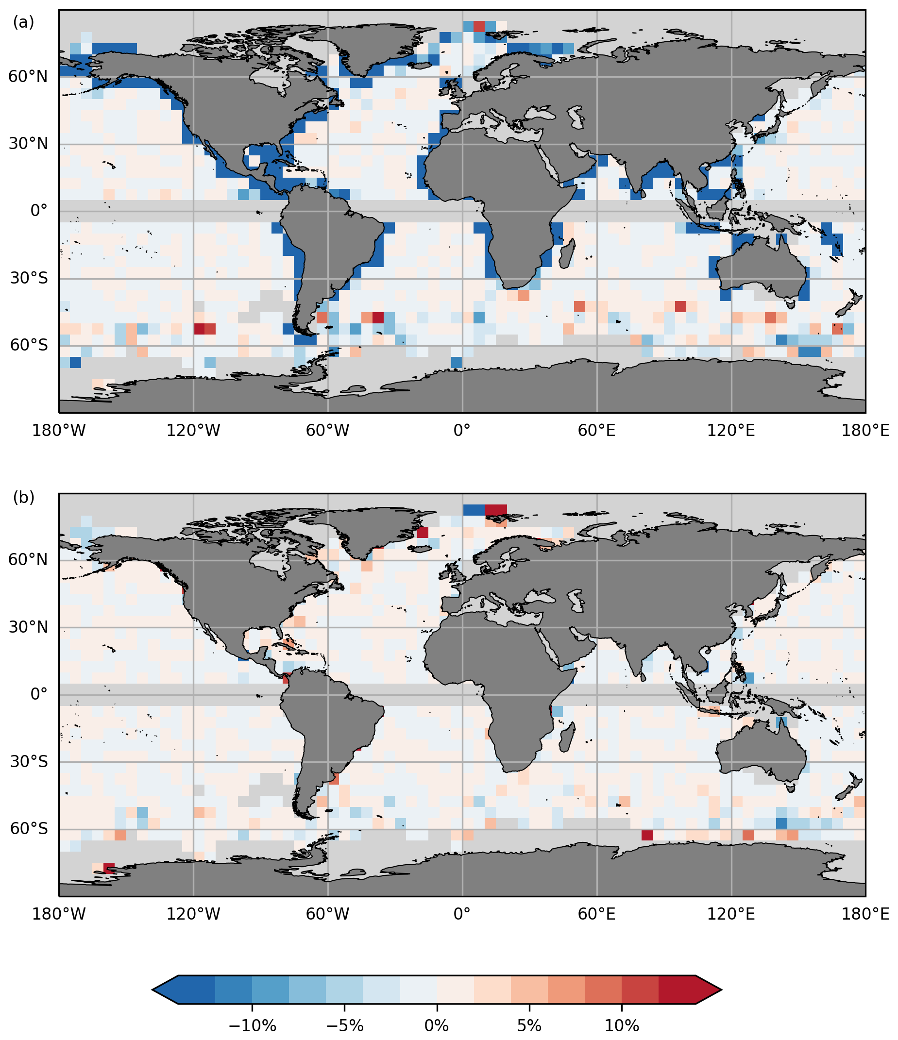
Figure 1 Comparison of the RMS of the differences (a) in current modulus and (b) in direction, of the independent drifting buoy velocities and the altimeter geostrophic velocities obtained using CNES-CLS22 MDT first guess (not applying the lagrangian coastal filtering) and CNES-CLS18 MDT first guess, in percent: $\mathit{\%}\mathrm{RMSD}=\mathrm{RMS}\left(U_{{\mathrm{MDT}}_{\mathrm{FG}\mathrm{22}}}\right)-\mathrm{RMS}\left(U_{{\mathrm{MDT}}_{\mathrm{FG}\mathrm{18}}}-U_{\mathrm{d}}\right)/$ $\mathrm{RMS}\left(U_{{\mathrm{MDT}}_{\mathrm{FG}\mathrm{18}}}-U_{\mathrm{d}}\right).$ These statistics are calculated in boxes of 5° by 5°. Only boxes with more than 100 measurement points and more than 10 different drifters are shown. The bluish colors denote improvement while reddish colors stand for degradation.

3.2 Computation of the synthetic mean heights

The estimation of synthetic mean heights aims to reproduce the physical content of the Mean Dynamic Topography (MDT) using temperature and salinity ($T/S$) profiles. Dynamic heights are computed relative to various reference depths (200, 400, 900, 1200, and 1900 m), capturing the baroclinic component of ocean dynamic height. These estimates lack contributions from deeper baroclinic and barotropic processes, the method used is described by Rio et al. (2011) and also used by Rio et al. (2014a) and by Mulet et al. (2021) and enables the estimation of the missing components. Associated errors are computed as described in Rio et al. (2011). The optimal analysis is then performed with anomalies relative to the MDT first guess, which is later restored to obtain the final MDT. This approach isolates the synthetic dynamic heights small scale structures. The resulting synthetic mean height anomalies reveal strong signals in major ocean currents, such as western boundary currents and the Antarctic Circumpolar Current, where anomalies exceed ±10 cm. These anomalies will result in enhanced geostrophic slopes, thereby accelerating large-scale oceanic currents.

3.3 Computation of the synthetic mean velocities

Velocities measured from drifters (Sect. 2) and surface Argo float drifts are processed to obtain estimates of the geostrophic current associated with the MDT. This is achieved by removing from the drifter velocities the ageostrophic components of the current, as well as the temporal variability of the geostrophic component of the velocities:

$$\begin{array}{}\text{(1)}& \begin{array}{rl}{U}_{\mathrm{synth}}& =U_{\mathrm{drifter}}-U_{\mathrm{Ekman}}-U_{\mathrm{Stokes}}-U_{\mathrm{inertial}}-U_{\mathrm{tidal}}\\ & -U_{\text{ageo-hf}}-U_{\mathrm{slippage}}-U_{\mathrm{alti}}^{\prime }\end{array}\end{array}$$

First, wind-driven currents (U_Ekman) are removed from the drifter velocity, as well as the wind slippage (U_slippage), which is the direct effect of wind on undrogued drifters. U_Ekman is taken from the Copernicus-Globcurrent product (MULTIOBS_GLO_PHY_REP_015_004, Global Total (COPERNICUS-GLOBCURRENT), Ekman and Geostrophic currents at the Surface and 15m | Copernicus Marine Service, https://data.marine.copernicus.eu/product/MULTIOBS_GLO_PHY_MYNRT_015_003/description last access: 11 March 2026) while wind slippage correction (U_slippage) is available in the CMEMS INSITU_GLO_PHY_UV_DISCRETE_MY_013_044 product (https://data.marine.copernicus.eu/product/INSITU_GLO_PHY_UV_DISCRETE_MY_013_044/description, last access: 11 March 2026). These products are consistent as they use same inputs for computation: ERA5 wind and wind stress (Sect. 3) and Mixed Layer Depth as a proxy to the Ekman layer thickness (from CMEMS ARMOR3D: MULTIOBS_GLO_PHY_TSUV_3D_MYNRT_015_012, https://data.marine.copernicus.eu/product/MULTIOBS_GLO_PHY_TSUV_3D_MYNRT_015_012/description, last access: 11 March 2026). Then the temporal variability of the geostrophic component of velocities ($U_{\mathrm{alti}}^{\prime })$ is removed. Next, the tide, inertial oscillations and residual ageostrophic signal (as U_stokes) are removed by high-frequency filtering. Finally, the mean synthetic velocities obtained are averaged in boxes $\mathrm{1}/\mathrm{8}$° by $\mathrm{1}/\mathrm{8}$°.

This method i.e. the estimation of the wind-driven component of the current and slippage, and the filtering applied are fully described by Mulet et al. (2021, Sect. 5) and builds on previous work by Rio and Hernandez (2004), Rio et al. (2007, 2011, 2014a).

Associated errors are estimated within each $\mathrm{1}/\mathrm{8}$° by $\mathrm{1}/\mathrm{8}$° bin by combining several elements. First, individual velocity error estimates are computed as the sum of two contributions: the altimetric velocity anomaly errors – equal to 40 % (50 %) of the temporal variance of the zonal (meridional) component, following Le Traon and Dibarboure (1999) – and the geostrophic velocity error of the drifters, which depends on the platform type (SVP-type drifters drogued or undrogued or Argo floats). Second, the variance within each bin where the synthetic mean velocities are calculated provides a proxy for the error associated with residual ageostrophic signals and remaining temporal variability.

For each bin, the final error is defined as the maximum of these two contributions divided by the number of observations, following the methodology described in Rio et al. (2011, 2014b). The resulting error magnitude depends on the local sampling density; in practice, the standard errors of the zonal and meridional components typically fall within the range of 2–30 cm s⁻¹, with lower values in well-sampled regions and higher values in dynamically energetic areas. These ranges are consistent with the global statistics later summarized in Table 1.

For this new MDT, we are also using surface velocity data from High Frequency radars located in the Mid Atlantic Bight region of the East Coast of the USA, from Cape Hatteras to Cape Cod (Fig. 2 shows the spatial coverage of the HF radar data used, (6 km by 6 km resolution). In the same way as for drifter data, these velocities are processed to extract the information they hold on the mean geostrophic velocity associated with MDT. We used the cleaned, detided, high-frequency filtered mean currents for the period 2006–2016 processed by Rutgers University (Roarty et al., 2020). The mean wind-driven currents over the same period (U_Ekman taken from the Copernicus-Globcurrent product MULTIOBS_GLO_PHY_REP_015_004) were removed. Finally these mean currents were re-referenced to the 1993–2012 period using the following equation, applied by Caballero et al. (2020): $U_{\mathrm{HFR}}^{\text{1993–2012}}=U_{\mathrm{HFR}}^{\text{2006–2016}}-{〈U_{\mathrm{SLA}}〉}_{\text{2006–2016}}$; where $U_{\mathrm{HFR}}^{\text{1993–2012}}$ and $U_{\mathrm{HFR}}^{\text{2006–2016}}$ denote the geostrophic mean velocities from HF radar referenced to the 1993–2012 and 2006–2016 periods, respectively, and ${〈U_{\mathrm{SLA}}〉}_{\text{2006–2016}}$ represents the mean geostrophic current anomalies associated with SLA, referenced to 1993–2012, averaged over 2006–2016.

Velocity datasets from drifting buoys and HF radars were integrated as two separate datasets for multivariate objective analysis. The error associated with HF radar data was set as a constant across the entire domain: 6.0 cm s⁻¹ for the U component and 5.7 cm s⁻¹ for the V component. Initial tests using spatially varying errors based on HF radar current variability revealed patterns linked to the measurement system, such as higher variability “stripes” depending on radar distance. To avoid introducing instrument-related artifacts, a constant error equal to the spatial mean of the cell-wise standard deviations was adopted. For drifter data, errors range from a few cm s⁻¹ on the continental shelf to about 20 cm s⁻¹ in the Gulf Stream.

Figure 2 shows these mean synthetic velocities estimated from (a) drifters (at $\mathrm{1}/\mathrm{8}$° resolution) and (b) HF radar, over the Mid Atlantic Bight area off New Jersey and Delaware (USA). The figure also shows the 100 and 2000 m isobaths that define the extent of the continental shelf. The average velocities estimated by drifters are noisier and more intense than those estimated from HF radars. It is worth noting that there are very few drifter observations over the continental shelf in the Mid-Atlantic Bight and, more generally, over continental shelves worldwide. This scarcity of data may explain why currents derived from drifter measurements appear noisier compared to those obtained from HF radar observations. And this intensity is consistent with the tendency of drifters to accumulate in the shelf-break where currents are strong. Both maps show recirculation to the south-east at the 100 m isobath. The drifters (Fig. 2a) show this current as narrow and intense (15 to 20 cm s⁻¹), whereas the HF radars (Fig. 2b) show a broad current of between 5 and 10 cm s⁻¹. Very close to the coast, velocities are generally low (below 5 cm s⁻¹), but currents can be perpendicular to the coast (e.g. Fig. 2b at 74.5, 75 and 75.5° W). Outflow from the Delaware Estuary could explain cross-shore currents near 38.5° N, though this is also near the baseline of the HF radar sites where directional accuracy is diminished.

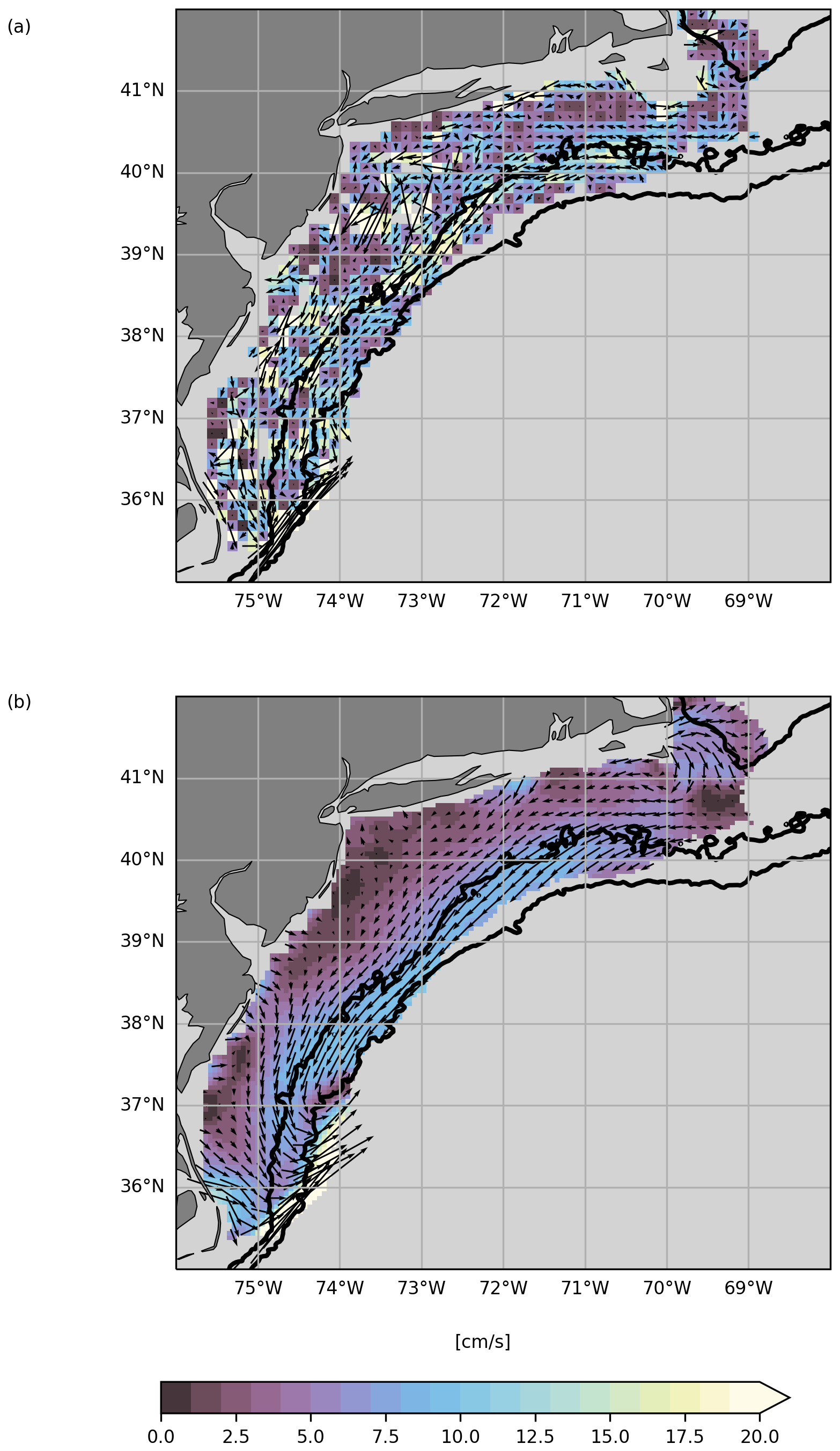
Figure 2 Synthetic mean velocities in the Mid Atlantic Bight region off New Jersey and Delaware, estimated (a) from drifting buoy (at $\mathrm{1}/\mathrm{8}$°) and (b) from HF radar data (6 km by 6 km resolution). The HF radar data mask was applied to the drifter data for a comparison of the two datasets. Black lines represent 100 and 2000 m isobaths.

3.4 Multivariate objective analysis

The third step of this method is multivariate objective analysis as described by Rio and Hernandez (2004), Rio et al. (2007, 2011, 2014a) and by Mulet et al. (2021), which uses the synthetic mean geostrophic velocities and synthetic mean heights to improve the first guess, in particular to improve the fine scales, to obtain the CNES-CLS22 MDT. This optimal analysis requires the a priori MDT variance and the a priori zonal and meridional spatial correlation scales of the estimated field. The same statistical a priori as for Rio et al. (2014a) and Mulet et al. (2021) are used here. In the equatorial bandwhere the geostrophic approximation is no longer valid, only mean synthetic height observations are used for MDT estimation, and only mean synthetic velocities observations are used for current inversion.

4 Results

4.1 High-resolution CNES-CLS2022 MDT and associated currents

The CNES-CLS22 MDT obtained is shown in Fig. 3a and the magnitude of the associated geostrophic currents is displayed in Fig. 3b. Compared with the first guess, the CNES-CLS22 MDT contains more small scales, gradients are sharper, and currents are accelerated. Figure 4 also shows a zoom of this new CNES-CLS22 MDT (a) and the geostrophic current magnitude (b) over the Arctic zone, as well as a zoom of the CNES-CLS18 MDT (c) and currents (d). Firstly, we note that the CNES-CLS22 MDT covers the Arctic zone, which was not the case before. This is due to the improved coverage of the CNES-CLS22 MSS used to estimate the first guess of this new MDT. Artifacts present on the CNES-CLS18 MDT have disappeared from the new version, for example around 110–120° E. Moreover, Beaufort gyre is better resolved, and Pan-Arctic transport is visible. On the other hand, the Beaufort Gyre tends to “spread out” over the Canadian Archipelago, which is not physical. This unrealistic spreading is primarily linked to weaknesses in the CNES-CLS22 MSS in this region, as noted by Schaeffer et al. (2023). The MSS suffers from a loss of valid observations, particularly CryoSat-2 SARin mode data in this area. Uncertainties are directly linked to observational coverage: they remain low in regions with dense sampling, whereas they increase substantially where $T/S$ profiles or drifter velocities are scarce. This dependence on data availability is a structural limitation of the method, particularly evident on continental shelves and at high latitudes.

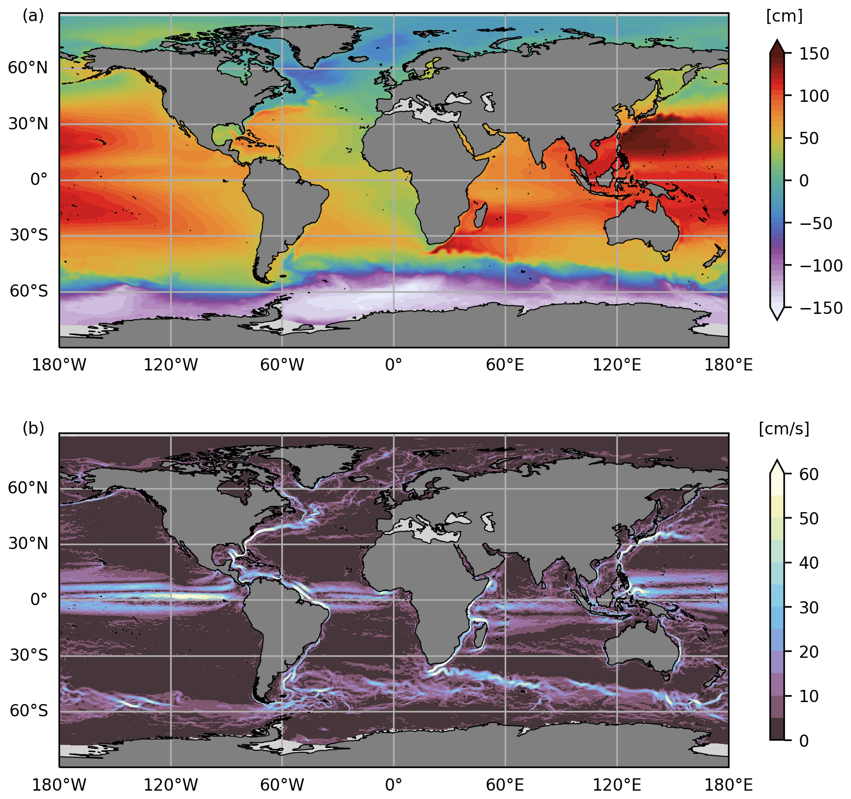
Figure 3 (a) The CNES-CLS22 MDT (cm) and (b) and the amplitude of the geostrophic currents associated with this MDT (cm s⁻¹).

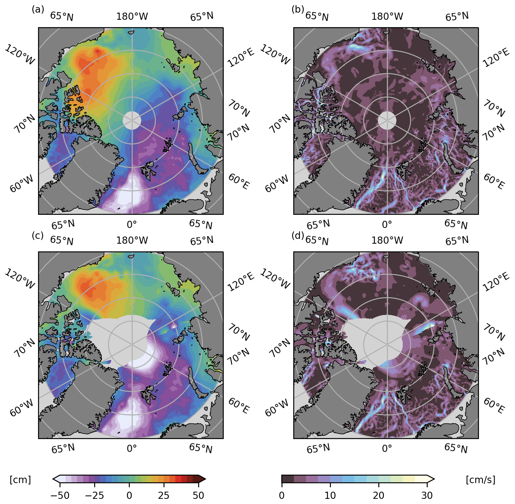
Figure 4 Zoom in on the Arctic zone of (a) the CNES-CLS22 MDT (in cm), (b) the amplitude of the associated geostrophic currents (in cm s⁻¹), (c) the CNES-CLS18 MDT (in cm) and (d) the amplitude of the geostrophic currents associated with the CNES-CLS18 MDT (in cm s⁻¹).

To look at the energy content of geostrophic currents associated with MDT, different MDT solutions were compared through a spectral analysis: the first guess (called FirstGuess22), the previous CNES-CLS13 MDT (referenced over the 1993–2012 period), the previous CNES-CLS18 MDT (Mulet et al., 2021), the DTUUH22 MDT (based on a combined geoid and enhanced with drifter data for high resolution, Knudsen et al., 2022), the new CNES-CLS22 MDT and the Glorys12 numerical model MDT ($\mathrm{1}/\mathrm{12}$° numerical model from Mercator-Ocean and distributed within CMEMS: product GLOBAL_REANALYSIS_PHY_001_030, https://data.marine.copernicus.eu/product/GLOBAL_MULTIYEAR_PHY_001_030/description, last access: 19 March 2026).

Figure 5 shows spectral analysis for the northward component of mean geostrophic current (noted Vg) associated with MDTs, in the Antarctic Circumpolar Current area, between 0 and 110° E and between 37 and 64° S. The Vg-CNES-CLS22 (in black) has significantly more variance than the first guess (noted Vg-FirstGuess22, in dashed blue) on scales from 1000 km to the smallest, and it is the in-situ data that increases the variance on these scales. The synthetic fields derived from in situ data are primarily intended to introduce small-scale variability, but they also correct large-scale structures, for example by intensifying major geostrophic currents, which is reflected in the spectra. The energy of the first-guess curve decreases significantly at scales smaller than 200 km. The three CNES-CLS MDTs (13 in yellow, 18 in red and 22 in black) follow the variance level and spectral slope of the GLORYS12 model (in green), up to about 200 km for the CNES-CLS13 MDT, and up to around 150 km for the CNES-CLS18 and the CNES-CLS22 MDT. At the smallest scales, there is a variance decay with the same slope toward the smallest scales. The energy decay slope of CNES-CLS22 and CNES-CLS18 MDTs is steeper than that of GLORYS but less steep than that of CNES-CLS13 MDT. It remains fairly regular down to 40 km, where it flattens, likely corresponding to a noise plateau, similar to what is observed below 30 km for GLORYS12. The regular energy loss of CNES-CLS22 and CNES-CLS18 MDTs appears physically consistent, but these solutions may be contaminated by noise at scales below 40 km (where the energy decay slope becomes weaker). This noise likely originates from in situ observations, from residual ageostrophic signals or poorly corrected temporal variability.

Figure 5 also shows the spectrum of the DTUUH22 MDT (in dashed pink), whose energy curve decreases more rapidly than that of GLORYS12 below 600 km scales, reaching a level similar to first-guess22 and then flattening into a noise plateau between about 125 and 50 km.

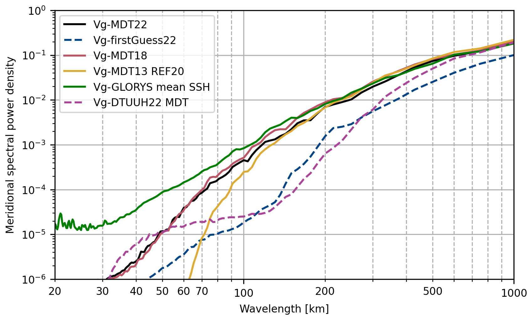
Figure 5 Spectral Power Density calculated on northward component of geostrophic current associated with different MDT solutions in the region 0–110° E, 64–37° S, in the Antarctic Circumpolar Current area for the meridional direction.

4.2 Validation

The validation of the CNES-CLS22 MDT is carried out using different approaches. First, this solution is evaluated qualitatively by region (the European Arctic and the Mid Atlantic Bight), then it is evaluated quantitatively with independent drifter data and then with independent height data estimated from $T/S$ profiles.

4.2.1 Qualitative validation

The European Arctic

As seen previously, the CNES-CLS22 MDT provides better coverage of the Arctic region and corrects various CNES-CLS18 artifacts. In this section, we take a closer look at the European Arctic region, and in particular the Yermak Plateau area where the Fram Strait branch of the Atlantic Water flow to the Arctic enters the Polar Basin (Fig. 7a), and the St. Anna Trough in the northern Kara Sea which is the main gateway for the Barents Sea branch of the Atlantic Water flow to the Polar Basin (e.g., Schauer et al., 2002, Rudels, 2015; Fig. 7d). We are looking at different solutions for these two areas. For the zoom on the Yermak Plateau, the new CNES-CLS22 MDT solution is shown in Fig. 7a with the bathymetric and geographic elements cited in this section, the CNES-CLS18 MDT solution is shown in Fig. 7b and in c the DTUUH2022 solution is shown. For the zoom on the St Anna Through, the CNES-CLS22 MDT solution is shown in Fig. 7d with the geographical elements mentioned, the CNES-CLS18 solution is shown in Fig. 7e and the DTUUH2022 solution in Fig. 7f. The first observation is that the DTUUH2022 solution is smoother than the two CNES-CLS solutions on these two zones.

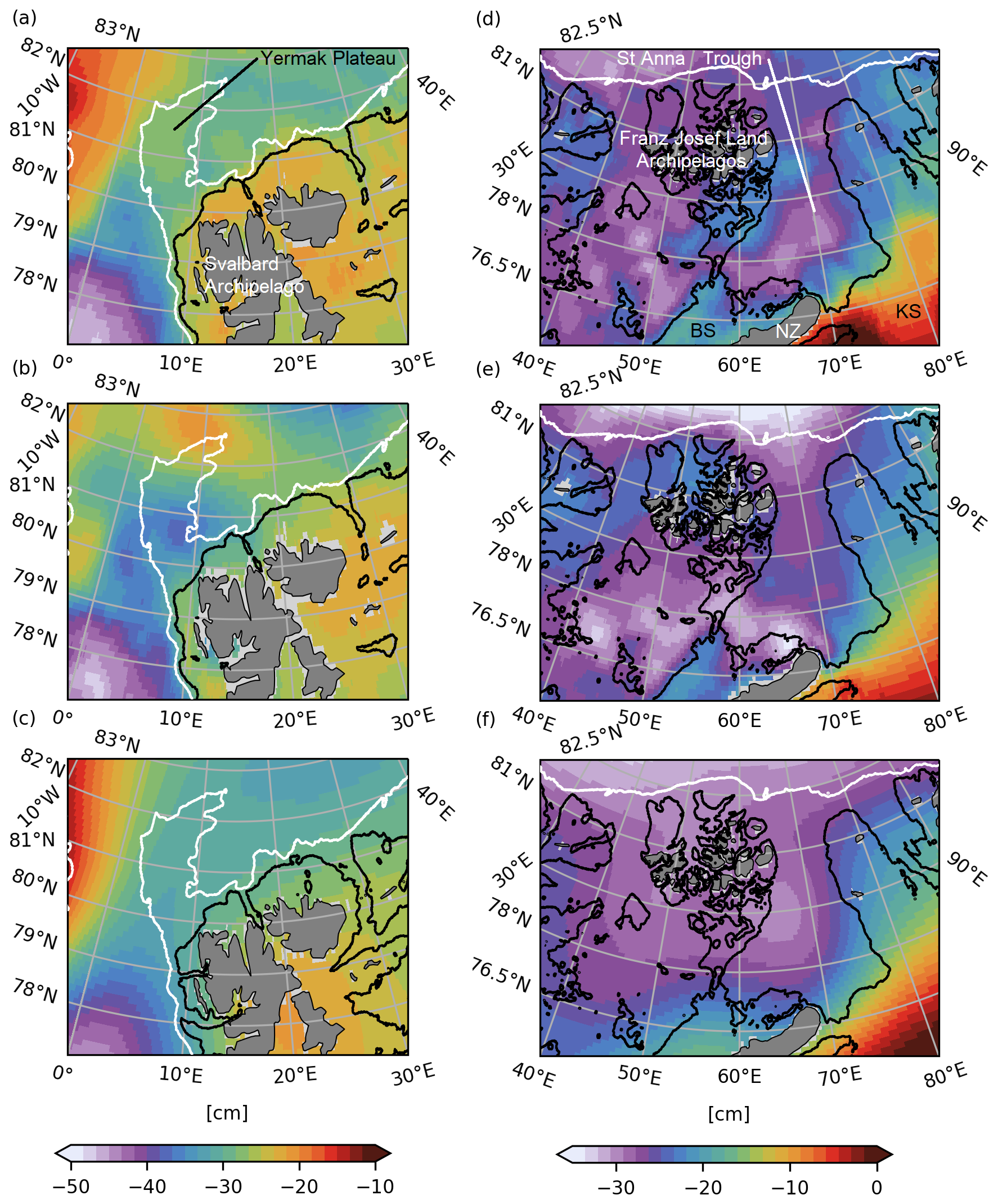
Figure 6 (a) CNES-CLS22 MDT, (b) CNES-CLS18 MDT and (c) DTUUH22 MDT in Yermak Plateau area. The white line represents the 1000 m isobath and the black line the 200 m isobath. Figure 7a shows the bathymetric and geographical features: the Yermak Plateau and Svalbard Archipelago. (d) CNES-CLS22 MDT, (e) CNES-CLS18 MDT and (f) DTUUH22 MDT in St Anna Through area. The white line represents the 1000 m isobath and the black line the 200 m isobath. Figure 7d shows the geographical features: the St Anna Through, the Franz Josef Land Archipelago, the Novaya Zemlya (NZ), the Barents Sea (BS) and the Kara Sea (KS).

In the Yermak Plateau area, where the Fram Strait branch of the Atlantic Water inflow enters the Polar Basin, the CNES-CLS22 MDT shows better alignment of the flow with the bathymetry both for the Svalbard branch crossing the plateau and the Yermak branch going around the plateau (see Fig. 1 in Meyer et al., 2017), compared with the CNES-CLS18 MDT and DTUUH22 MDT.

The CNES-CLS22 MDT also shows some improvements in the St. Anna Trough where the Barents Sea branch of the Atlantic Water flow to the Arctic exits the Barents Sea and enters the Polar Basin. Here, the CNES-CLS22 MDT better aligns with the bathymetry in the northeastern Barents Sea and northern Kara Sea compared with the CNES-CLS18 MDT and DTUUH22 MDT. Moreover, several more detailed differences also better align with features of the flow reported in the literature. The main flow from the Barents Sea is clearly aligned along the bathymetry in the southern part of the trough between the Novaya Zemlya and Franz Josef Land archipelagos (Schauer et al., 2002; Lien and Trofimov, 2013), and there is a clear indication of cyclonic circulation of the Fram Strait branch within the same trough (Gammelsrød et al., 2009; Lien and Trofimov, 2013). There is also an indication of a continuous Coastal Current along the northern tip of Novaya Zemlya (Lien and Trofimov, 2013), which is not clearly seen in the CNES-CLS18 MDT and DTUUH22 MDT. Further north in the St. Anna Trough the CNES-CLS22 MDT shows better alignment of the flow with the bathymetry (e.g., Dmitrenko et al., 2015) compared with the smoother DTUUH22 MDT, in addition to more distinct features not seen in the CNES-CLS18 MDT or DTUUH22 MDT. At 81N, there is an indication of a cyclonic eddy previously identified by hydrographic observations, likely caused by the Fram Strait branch entering the St. Anna Trough (Osadchiev et al., 2022). Moreover, a bathymetric feature to the east of the Franz Josef Land archipelago likely affects the southward flowing part of the Fram Strait branch and causes an anti-cyclonic flow as shown in the CNES-CLS22 MDT.

Mid Atlantic Bight

As seen in Sect. 2.3, the CNES-CLS22 MDT integrates synthetic geostrophic velocities estimated from high-frequency radar velocities in the Mid Atlantic Bight (MAB) area on the east coast of the USA between Cape Cod and Cape Hatteras. In this section, the CNES-CLS22 MDT is looked at more precisely in the MAB and the adjoining region just north of the Gulf Stream where southwestward flow in the MAB coastal ocean crosses isobaths to depart the continental shelf and join a recirculation in the Slope Sea (Fig. 7b).

Figure 7 shows the contours of the CNES-CLS22 MDT (d) in comparison with the CNES-CLS18 MDT (c) and a ROMS model MDT (a). The ROMS model MDT (Fig. 7a) is an average from the ROMS model used in a climatological diagnostic configuration to calculate a kinematically (coastline and bathymetry) and dynamically (ROMS nonlinear model physics) consistent circulation constrained by mean observations of the ocean state and forced by mean surface fluxes and river inflows (details given in Wilkin et al., 2022).

Lentz (2008) and Zhang et al. (2011) have advanced arguments as to the magnitude of the along-shelf sea level gradient in the MAB necessary to complete a momentum balance. We expect gentle southwestward flow throughout the Mid Atlantic Bight, and certain recirculation features in the Gulf of Maine, and encircling Georges Bank that are clearly evident in the ROMS MDT (Fig. 7a). The across-shelf sea level gradient is consistent with observed southwestward mean currents. Furthermore, the known pattern of geostrophic coastal currents requires that the MDT contours be largely parallel to the coast, which is the case with the ROMS MDT and not always the case with the CNES-CLS18 (Fig. 7c) and 22 (Fig. 7d) MDTs.

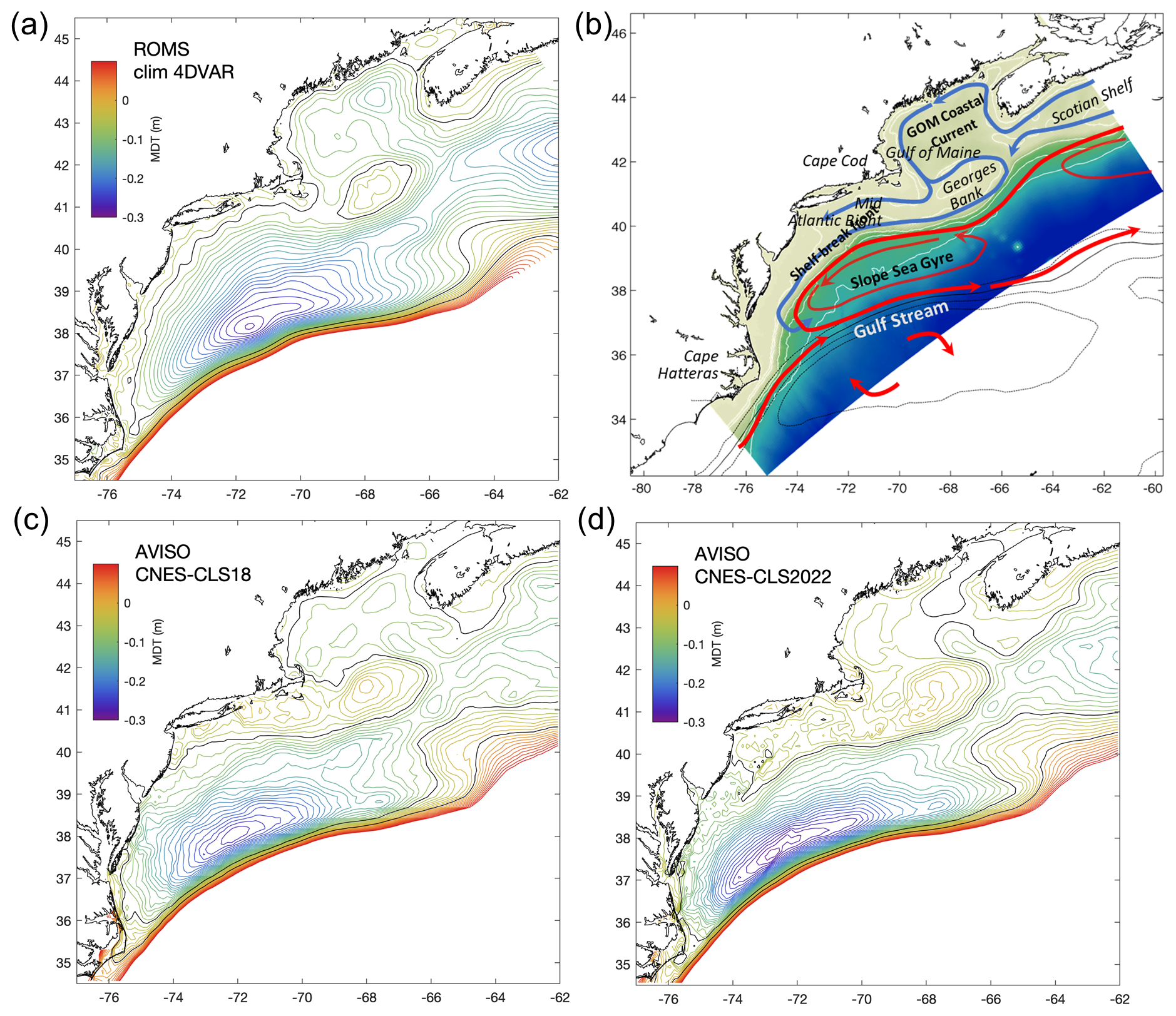
Figure 7 (a) ROMS model MDT contours, (b) Mid Atlantic Bight circulation, (c) CNES-CLS18 MDT contours and (d) CNES-CLS22 MDT contours. Black lines represent MDT contours at 0.05 and −0.05 m.

CNES-CLS18 MDT (Fig. 7c) shows a slightly more organized circulation on the shelf, although contours on the inner shelf are noisy. Coastal currents in the Gulf of Maine and Scotian Shelf emerge, but are weak. In addition, there are still MDT contours strongly intersecting the coast, which implies an unphysical geostrophic surface current normal to the coast and sea-level slope inversions along the shelf when sea level at the coast is expected to decrease monotonically toward the south on the basis of along-shelf momentum balance arguments.

The CNES-CLS22 MDT (Fig. 7d) remains noisy on the continental shelf, and there are still contours cutting the coast (associated with low geostrophic velocities). Coastal currents on the Scotian Shelf are more organized, but there are still flows into the coast of central New Jersey. And in the Gulf of Maine the CNES-CLS18 MDT is more consistent with the ROMS model, and the circulation of CNES-CLS18 MDT around the Georges bank seems more realistic than the circulation of CNES-CLS22 MDT. While CNES-CLS22 represents progress, further refinement is needed to achieve physically consistent MDT near broad shelves. It should be noted, however, that model-based MDTs are not absolute truth. It is therefore necessary to exercise caution when interpreting improvements based solely on model comparisons, as this also illustrates the difficulty of validating MDTs over continental shelves. These discrepancies highlight that MDT estimation over shelves remains problematic, even with HF radar integration. The geostrophic assumption is less valid in shallow regions dominated by tides and wind-driven flows, and the lack of shallow hydrographic data further limits physical consistency.

Impact on the Atlantic Water pathways

Atlantic Water (AW) transported to the Arctic Ocean through the Nordic Seas plays a major role in the global climate system. The heat and salt are transported to the Nordic Seas by the Norwegian Atlantic Current (NwAC), a two-branch current system, of which the eastern branch, the Norwegian Atlantic Slope Current (NwASC) follows the shelf edge as a barotropic slope current, while the western branch, the Norwegian Atlantic Front Current (NwAFC) follows the western rim of the Norwegian Sea as a topographically guided frontal current. Further downstream in the Norwegian Sea, the NwAFC and the NwASC, respectively, form the western and eastern boundaries of the Lofoten Basin, which is the most eddy active region in the entire Nordic Seas. There is no mean flow into the basin and the heat and salt are transported into the basin interior by the mesoscale eddies (Raj et al., 2016, 2020). The quasi-permanent anticyclonic eddy the “Lofoten Vortex” situated in its western part is the most distinct feature in the Lofoten Basin (Raj et al., 2015). Further downstream, the NwAFC flows along the Mohn Ridge while the NwASC continues along the continental slope, partly branching into the Barents Sea, and flows northwards as the West Spitsbergen Current.

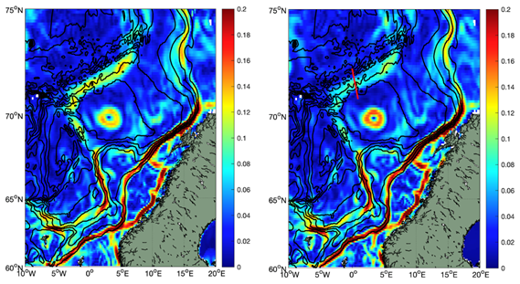
Figure 8 Mean geostrophic speeds (m s⁻¹) derived from: CNES_CLS22 MDT (left panel); and CNES_CLS18 MDT (right). The red line in the right panel indicates the location of the transect shown in Fig. 10. Isobaths are drawn in black.

The circulation of the Nordic Seas has been the subject of investigations since the Norwegian North-Atlantic Expedition in 1876–1878 (Mohn, 1877; Helland-Hansen and Nansen, 1909). Monitoring of AW heat transport in the Nordic Seas is mainly performed using numerical ocean model data (Copernicus Arctic Marine forecasting Services; ARC-MFC) and current meters located at the Iceland Faroe Ridge, the Faroe Shetland Channel, the Svinøy section, and in the Fram Strait. In comparison, Earth observations (EO) from satellites are under-exploited, even though satellite radar altimeters have provided continuous spatial coverage over the region for more than 30 years. The launch of the Gravity field and steady state Ocean Circulation Explorer (GOCE) mission in 2009, together with the implementation of better retrieval algorithms for the satellite altimeter data processing, has improved our ability to better monitor the ocean circulation (Johannessen et al., 2014). Based on these improvements, Raj et al. (2018) demonstrated the significant value of satellite derived surface velocities for monitoring long term variability of the circulation of AW in the Nordic Seas. Here, we assess the capability of the CNES-CLS22 MDT in better resolving the circulation of the region.

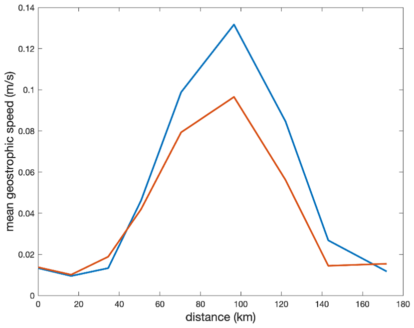
Figure 9 The mean geostrophic speed derived from CNES-CLS22 MDT (blue) and CNES-CLS18 MDT (red) across the Mohn Ridge (location of the transect shown in Fig. 9).

Figure 9 shows that both CNES-CLS22 MDT and CNES-CLS18 MDTs reproduce the two-branch structure of the Norwegian Sea circulation. The NwASC tightly follows the topography, intensifies at Svinøy and near the eastern border of the Lofoten Basin and due to topographic steering. Along the NwAFC, topographic steering induced intensification of the current is prominent at the western slope of the Vøring Plateau. The main improvement of the CNES_CLS22 MDT derived current estimates are along the western border of the Lofoten Basin and the Mohn Ridge. All previous versions of the MDT produced so far were not able to reproduce the NwAFC in this region correctly. Figure 10 shows that the difference can even reach up to 4 cm s⁻¹. On the other hand, the mean speed of the Lofoten Vortex derived from CNES-CLS22 MDT is comparatively lower than the one derived from the CNES-CLS18 MDT. All, in all, the results from CNES-CLS22 MDT are promising.

4.2.2 Regional quantitative validation

Comparison with ADCP in the Faroe-Shetland Channel

The Faroe-Shetland Channel (FSC; Fig. 10a), situated between the Shetland shelf to the east and the Faroe plateau to the west (Chafik, 2012), is a crucial passage for the global overturning circulation (Hansen and Østerhus, 2000; Chafik et al., 2020). The region hosts northward flow of warm North Atlantic water carried by the Slope Current toward the Nordic Seas and the Arctic Ocean (Chafik et al., 2015), and the southward branch of the densest overflow water produced at higher latitudes (Chafik et al., 2023). The FSC is also partially supplied from north of the Faroes by the inflow of warm waters through the Iceland-Faroe Ridge (Poulain et al., 1996; Rossby et al., 2018), which recirculates in the channel before merging with the Slope Current (Poulain et al., 1996; Berx et al., 2013), as illustrated in Fig. 11a. Two essential components thus must be included in the MDT for an accurate representation of the mean circulation in the region: the bathymetrically constrained Slope Current to the east as well as the strong recirculation that traces the morphology of the FSC (Fig. 10a–b).

Figure 10c–d compares the two MDT solutions in the region and validate these against ship-mounted ADCP velocities across the FSC (Rossby and Flagg, 2012; Rossby et al., 2018; data available on: http://po.msrc.sunysb.edu/Norrona/, last access: 11 March 2026) on Fig. 10e–f. The differences between CNES-CLS22 and CNES-CLS18 MDTs are primarily at large scales (Fig. 10d), mostly driven by the first-guess fields, which rely on different MSS and geoid solutions. The CNES-CLS22 MDT represents the large-scale circulation in the eastern subpolar North Atlantic as well as the FSC (see, e.g., Childers et al., 2015; their Fig. 7). Notably, the spatial structure of the highlighted −0.15 m contour (Fig. 10c, blue contour) in the CNES-CLS22 MDT closely follows the bathymetry and passes directly through the FSC entrance, suggesting a more accurate depiction of the inflow of warm Atlantic waters into the channel (cf. Fig. 10a). In contrast, the −0.15 m contour in the CNES-CLS18 MDT (Fig. 10c, red contour) exhibits unrealistic deviations, especially near the FSC entrance, where it overshoots into the Faroe shelf and misses the channel entrance. Due to this unrealistic overshoot in CNES-CLS18, there is a pronounced negative difference between the two MDT solutions in the southwestern part of the FSC, particularly over the Faroe shelf (Fig. 10d). However, the CNES-CLS22 MDT introduces a distortion by deflecting the path of the Slope Current into the channel interior in the northeastern FSC (Fig. 10d). This results in a pronounced positive difference compared to CNES-CLS18 MDT, where the contours are more closely aligned with the bathymetry, indicating a stronger topographic control of the northward-flowing warm waters.

Because of a more realistic Slope Current in CNES-CLS MDT18, its velocities normal to the FSC are found to closely match the ADCP estimates as compared to CNES-CLS MDT22 (Fig. 10e), where the northward flow is less confined to the slope and spread out over a larger area across the channel (see also Fig. 10c). This behaviour may be due to a restricted and too narrow recirculation on the Faroe slope, as indicated by the −0.2 m contour (see Fig. 10c). To further illustrate this point, we estimate the cumulative transport across the FSC. For simplicity, we assume a barotropic velocity structure over the upper 400 m layer (see e.g., Rossby and Flagg, 2012). Figure 10f shows a good agreement between the CNES-CLS MDT18 net northward transport of 2.9 Sv and the ADCP-based estimate. In contrast, the CNES-CLS MDT22, which is characterized by a broad or diffuse Slope Current, significantly overestimates the net northward transport at 5.5 Sv.

We conclude that in this area, the CNES-CLS MDT22 appears to perform worse than the CNES-CLS MDT18, and the differences between the two are mainly at large scale, likely linked to the first guess, which seems less accurate. Adding in situ data does not improve accuracy in regions with narrow currents and strong recirculations. The challenge in accurately constraining the path of the sharp Slope Current may arise from misrepresentations of the recirculating waters within the FSC. Other contributing factors could include inaccuracies in the representation of the surrounding shelf regions that border the FSC.

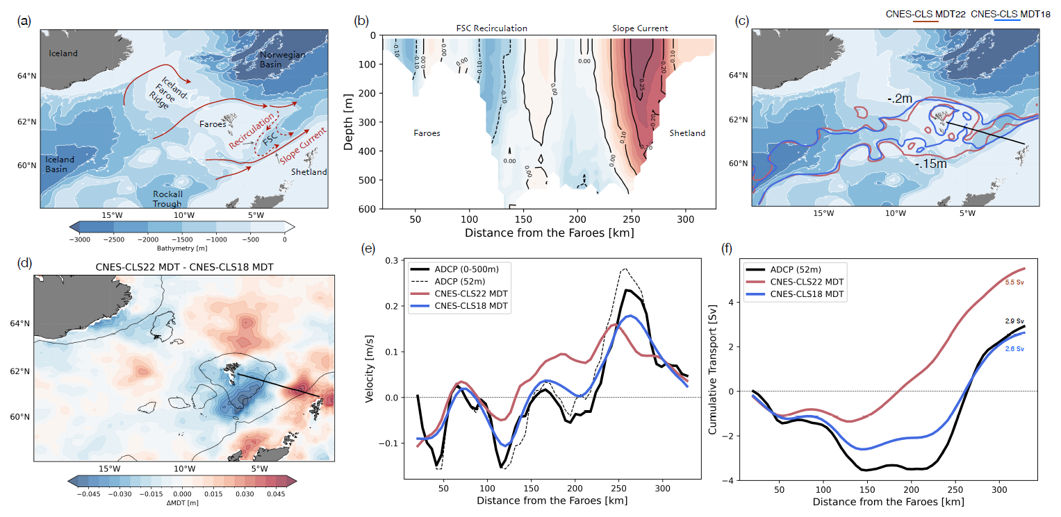
Figure 10 (a) Bathymetric map including a schematic of upper-ocean circulation in the region. The Slope Current and the recirculation in the Faroe-Shetland Channel (FSC) are indicated. Bathymetric contours are shown at depths of 500, 1000, 1500, 2000, 2500, and 3000 m. (b) Time-mean (2008–2018) velocity structure across the FSC based on ship-mounted Acoustic Doppler Current Profiler (ADCP) between Shetland and the Faroe Islands (see section in panel (c)). The velocities are normal to the ship track. (c) Similar to panel (a), but showing the −0.15 and −0.2 m contours from two MDT solutions. (d) Regional difference between the two MDT solutions (CNES-CLS MDT22 minus CNES-CLS MDT18). (e) Normal velocities from the ADCP averaged over the upper 500 m (solid black line) and at 52 m depth (dashed black line), compared to CNES-CLS MDT22 (red) and CNES-CLS MDT18 (blue). (f) Cumulative transport integrated from west to east (starting from the Faroes) for the ADCP and both MDT solutions, with transport multiplied by 400 as a rough estimate of upper-ocean transport. For ADCP data, velocities at 52 m are used.

4.2.3 Quantitative validation with independent $T/S$ profiles

Here, CNES-CLS22 and CNES-CLS18 MDTs are compared with independent dynamic height data derived from $T/S$ profile observations since 2017 that were withheld from the analysis, as noted previously. Dynamic heights estimated from $T/S$ profiles omit the signal due to baroclinic processes occurring below the reference depth, and by barotropic processes, Therefore, for validation purposes we choose to keep only the deepest profiles (reference depth 1900 m) to minimize the omitted dynamic signal, which leaves us with a validation set of 2 % of the database.

As a first step, we compare the CNES-CLS18 and CNES-CLS22 MDTs against these independent dynamic heights by looking at the correlation of the ADT (SLA+MDT considered) and the independent dynamic heights (figures not shown). Correlations are calculated in boxes of 5° by 5° (with at least 20 data) and are high, mostly between 0.8 and 1 for both MDTs, and it is difficult to differentiate between them.

Secondly, Fig. 11a shows the mean bias per 5° × 5° box between the ADT estimated from the CNES-CLS22 MDT and the independent dynamic heights. This global mean bias is 1.30 m, with spatial variations in the Norwegian Sea and to the south near Antarctica (equivalent for CNES-CLS18, not shown) and mainly represents the barotropic component not observed by the dynamic heights. This is why it is removed from the estimate of mean synthetic heights for the calculation of the MDT and the following validation diagnosis on Fig. 11b shows a comparison between the variances of the differences (not considering the bias) between the different ADTs and the dynamic heights, in percent. In blue (in red), the variance of differences is reduced (increased) using CNES-CLS22 compared with CNES-CLS18.

Globally, we see an slight improvement in CNES-CLS22 MDT compared with CNES-CLS18 (average variance reduction of 0.5 %), but this is not true in all regions. South of the Atlantic and the Indian Ocean (as far south as Australia), the variance of differences is reduced for CNES-CLS22 by more than 10 % for many boxes (even if boxes of strong reduction are juxtaposed with boxes of increased variance of differences). Areas of degradation are concentrated in the north-western Atlantic, particularly south of Greenland, in the very north of the Pacific (along the Gulf of Alaska to the Fox Islands, and close to Russia) and in the south of the Pacific, where there are degradations of over 10 % (also juxtaposed with improvement boxes).

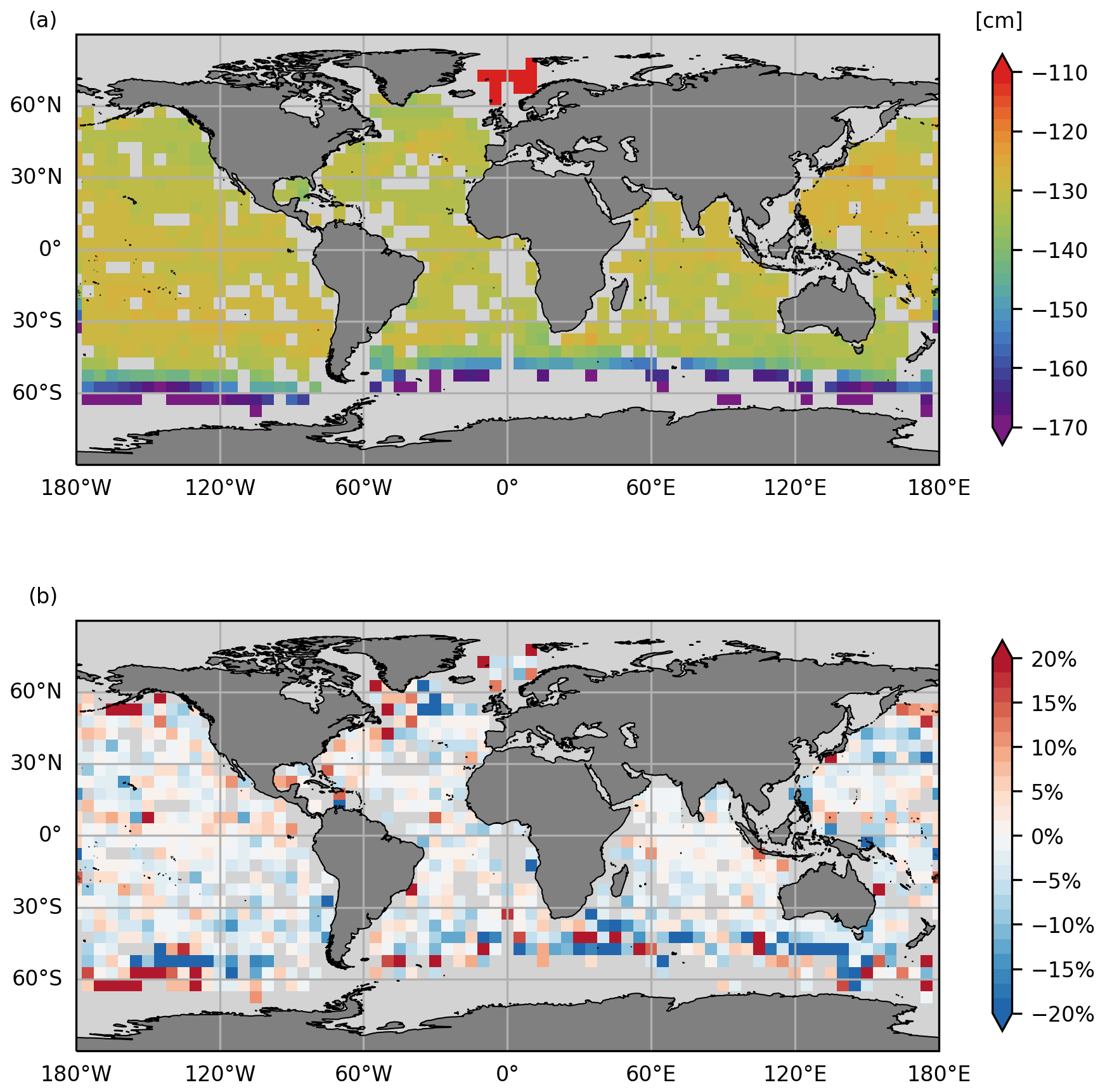
Figure 11 (a) shows the bias in centimetres between the dynamic heights estimated from the independent $T/S$ profiles and the ADT calculated from the CNES-CLS2 MDT. And (b) shows the reduction/increase in variance of the differences between independent dynamic heights and ADT (from CNES-CLS18 and CNES-CLS22) in percent. In blue (in red), the variance of differences is reduced (increased) using CNES-CLS22 compared with CNES-CLS18. All these statistics are calculated in 5° × 5° boxes, and only boxes with at least 20 data are kept.

4.2.4 Quantitative validation with independent drifters

Here, CNES-CLS18 and CNES-CLS22 solutions are compared with independent velocity data. 10 % of the AOML drifters dataset are randomly selected and kept for validation (independent data). These drifters are not evenly distributed across the oceans. There are few drifters close to Antarctica (south of about 50° S), at the equator, and in Arctic. In addition, the Atlantic is slightly better sampled than the other basins, and the North Indian Ocean less well sampled.

Following the same processing steps described previously, we remove the wind-driven current (Ekman and wind slippage) from total drifters current and then data are filtered at inertia frequency (if inertia frequency is between 1 and 5 d, otherwise take a minimum of 1 d and a maximum of 5 d) to remove the tide and inertial waves. The objective is to keep only the geostrophic signal. Geostrophy can't be used to estimate currents at the equator, so we exclude drifters between 5° S and 5° N.

Absolute dynamic topography values were calculated by adding the CMEMS gridded SLA to the new CNES-CLS22 MDT. Associated geostrophic currents were then derived and interpolated along the drifter trajectories. Bias and Root Mean Square differences (RMSD) between the obtained geostrophic velocities with CNES-CLS22 and CNES-CLS18 and the drifter derived geostrophic velocities were calculated spatially by 5° × 5° boxes. All these statistics are calculated with at least two different drifters and with at least 100 measurement points.

Comparisons of bias (a) in current modulus (in m s⁻¹) and (b) in direction (in degrees) are shown in Fig. 12. In blue (in red), there is a decrease (increase) in bias for geostrophic currents derived from the ADT estimated with the CNES-CLS22 MDT. Globally, there is a decrease in bias in current modulus (Fig. 12a) using the new solution, with a greater decrease in bias in areas of strong currents: Gulf Stream, Kuroshio, Agulhas Current and Antarctic Circumpolar Current. The areas of degradation are South Greenland and South Kerguelen. For the directional bias (Fig. 12b), the contribution of the new solution is more mixed, as the direction of geostrophic currents derived from the ADT using the CNES-CLS18 is better in the South between the Kerguelens and southern Australia. These remain areas with fewer validation drifters.

It is important to note that validation coverage is uneven across the globe. Drifter observations are sparse in the Arctic and Southern Ocean, and HF radar data are restricted to the Mid Atlantic Bight region. Furthermore, the validation using $T/S$ profiles relies on only ∼ 2 % of the dataset (deepest profiles), which limits the robustness of conclusions in poorly sampled areas. Users should therefore interpret CNES-CLS MDT22 results with caution in regions where in situ observations are scarce, as uncertainties remain higher in these areas.

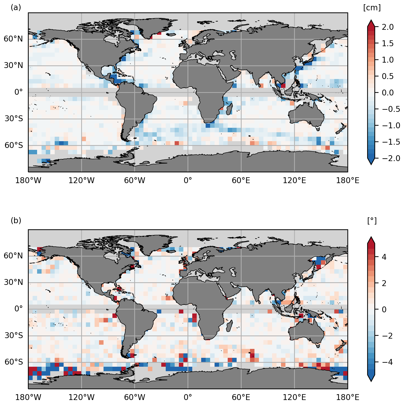
Figure 12 Comparison of bias (a) in current modulus and (b) in current direction independent drifting buoy velocities and the altimeter geostrophic velocities obtained using different MDT solutions. In blue (in red), the bias is reduced (increased) using CNES-CLS22 compared with CNES-CLS18.

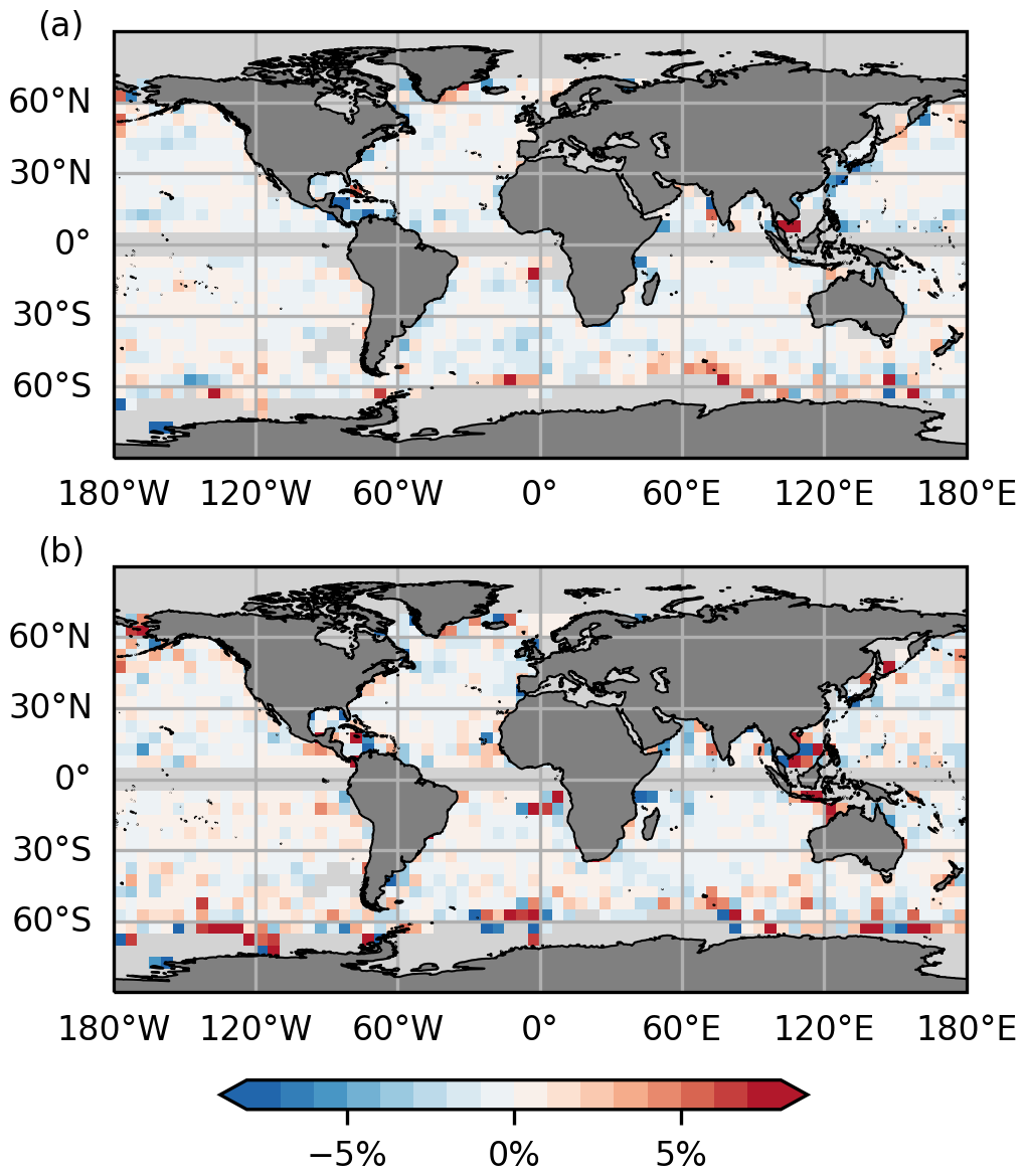
Figure 13 Comparison of the RMS of the differences (a) in current modulus and (b) in direction, of the independent drifting buoy velocities and the altimeter geostrophic velocities obtained using MDT solutions CNES-CLS22 and CNES-CLS18, in percent: $\mathrm{\%}\mathrm{RMSD}=\mathrm{RMS}\left(U_{\mathrm{ADT}\mathrm{22}}\right)-\mathrm{RMS}\left(U_{\mathrm{ADT}\mathrm{18}}-U_{\mathrm{d}}\right)/\mathrm{RMS}\left(U_{\mathrm{ADT}\mathrm{18}}-U_{\mathrm{d}}\right)$. In blue (in red), the bias is reduced (increased) using CNES-CLS22 compared with CNES-CLS18. All these statistics are calculated in 5° × 5° boxes, and only boxes with at least 2 drifters difters differents and at least 100 measurement points, are kept.

Comparisons of RMS of the differences (a) in current modulus and (b) in direction, of the independent drifting buoy velocities and the altimeter geostrophic velocities obtained using MDT solutions CNES-CLS22 and CNES-CLS18, in percent, are shown are shown on Fig. 13. In blue (in red), the RMSD is reduced (increased) using CNES-CLS22 compared with CNES-CLS18. In terms of current amplitude (Fig. 13a), the majority of boxes show an improvement of between 0 % and 2.5 % for the CNES-CLS22 solution, with a greater improvement at Kuroshio and in the Caribbean Sea. Areas of degradation in current amplitude RMS are the area around Kerguélen in the ACC and along the southeast coast of Greenland. Comparison of the RMS of differences in current direction (Fig. 13b) shows a more mixed result with degradation boxes compared to the CNES-CLS18 solution: in the ACC in the South Pacific. It can also be noted that some boxes show an improvement in the RMS of differences for the CNES-CLS22 solution in current amplitude but not in direction, and vice versa; this is the case for some boxes south of the Kerguélen Islands and at the extreme south of the Pacific. The areas around the Kerguélen Islands, in the South Pacific between −140 and −120° E, and around the Fox Islands in the extreme North Pacific remain areas of degradation in RMS of the differences in modulus and current direction for the new solution compared with the previous one. On the other hand, the Kuroshio, the North Atlantic and the Labrador Sea, as well as the Indian Ocean are areas where the RMS of the differences for the new CNES-CLS22 solution has improved compared to the CNES-CLS18 solution.

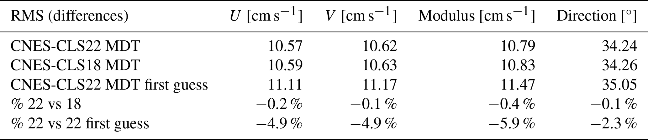
Globally, the two solutions CNES-CLS22 and CNES-CLS18 remain close with these drifter comparisons, as shown in the following Table 1, which summarizes the drifter comparison statistics over the whole area up to 70° N. Both solutions have a difference RMS of between 10.5 and 11 cm s⁻¹ for U and V components and current modulus, and a difference RMS of around 34° in direction. The comparison of the two solutions favours the new one, but by less than 1 %. It should also be noted that the comparison between the first guess and the CNES-CLS22 MDT shows an improvement in U and V of around 5 % in the RMS of differences, and an improvement of around 6 % in current amplitude and 2 % in direction, which is expected.

Table 1 RMS of the differences for the zonal component U, the meridional component V, the current modulus and the direction of the current, of the independent drifting buoy velocities and the altimeter geostrophic velocities obtained using MDT solutions CNES-CLS22, CNES-CLS18 and the CNES-CLS22 first guess. The last two lines show the reduction/increase in RMS of the differences between two solutions: CNES-CLS22 versus CNES-CLS18 and CNES-CLS22 versus CNES-CLS22 first guess, in percent (a negative percentage is a decrease in the RMS of the differences). These statistics were generated using all available drifters up to 70° N.

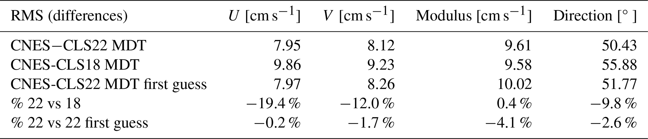
Given the small number of independent drifters in Arctic, this area is treated separately. Table 2 summarizes the RMS of the differences between the geostrophic currents derived from drifters (degraded treatment because SLA not available) and the geostrophic currents derived from ADTs calculated with the CNES-CLS22, CNES-CLS18 and background CNES-CLS22 solutions. The last two lines show in percent the reduction in RMS of the differences between CNES-CLS22 and CNES-CLS18 MDT and its first guess. In the zonal and meridional components of the current, the new solution reduces the RMS of the differences compared with the drifters by 19 % and 12 % respectively. This improvement translates into a clear improvement in direction of 9 %, which reduces the RMS of the differences from around 56 to 50°; but the RMS of the differences in current amplitude remains very slightly better for CNEs-CLS18. Note that, as the coverage is not quite identical, there are more points taken into account for CNES-CLS22 than for CNES-CLS18.

Table 2 RMS of the differences for the zonal component U, the meridional component V, the current modulus and the direction of the current, of the independent drifting buoy velocities and the altimeter geostrophic velocities obtained using MDT solutions CNES-CLS22, CNES-CLS18 and the CNES-CLS22 first guess. The last two lines show the reduction/increase in RMS of the differences between two solutions: CNES-CLS22 versus CNES-CLS18 and CNES-CLS22 versus CNES-CLS22 first guess, in percent (a negative percentage is a decrease in the RMS of the differences). These statistics are based on the Arctic zone north of 80° N. As the CNES-CLS18 MDT has a smaller coverage, the number of points used is slightly different for this solution than for the others.

5 Data availability

CNES-CLS22 MDT described in this manuscript can be accessed at https://www.aviso.altimetry.fr/en/data/products/auxiliary-products/mdt/mdt-global-cnes-cls.html (last access: 11 March 2026) under data DOI https://doi.org/10.24400/527896/A01-2023.003 (Jousset, 2023).

6 Conclusions

While CNES-CLS22 introduces methodological refinements and new data sources, the global improvement relative to CNES-CLS18 remains modest. Validation against independent drifter-based geostrophic velocities shows only ∼ 0.2 %–0.5 % reduction in RMS differences at the global scale (Tables 1–2). These gains, though statistically limited, are regionally significant – particularly in the Arctic and Nordic Seas, where coverage and physical consistency have improved markedly. CNES-CLS22 should therefore be considered a necessary incremental update, consolidating previous progress and enabling better representation of circulation in key regions, rather than a globally transformative revision.

The main improvement of this new CNES-CLS22 MDT over the previous CNES-CLS18 MDT is in the Arctic, with better coverage and a more physical solution (with the disappearance of artifacts from the previous version). Globally, the new CNES-CLS22 solution is close to the CNES-CLS18 solution, both have better resolution of small scales than previous CNES-CLS MDTs but are potentially polluted by noise at very short scales (< 40 km). At these small scales, the solution may introduce unrealistic mean kinetic energy. This noise likely originates from in situ observations, which raises an important point for future improvements: how to increase resolution using in situ data without excessively introducing noise into the final solution, for example from ageostrophic signals or poorly corrected temporal variability.

Improvements to this new MDT include a new first-guess with the CNES-CLS22 MSS and the GOCO06s geoid to which optimal filtering has been applied, as well as Lagrangian filtering at the coast to reduce the intensity of normal currents at the coast, drifting buoy and $T/S$ profile databases have been updated. The processing methodology for synthetic mean geostrophic velocities and synthetic mean heights remains unchanged, but it benefits from improvements in products as altimeter sea level anomaly, wind stress, and consequently Ekman currents and wind slippage.

A new data source – land-based HF radar surface current observations – was incorporated to extract physical content consistent with MDT in the Mid-Atlantic Bight region. Analysis of this area highlights that significant challenges remain in obtaining a physically consistent solution over continental shelves. On broad, shallow shelves, the first guess is often unreliable due to proximity to the coast, and these regions also suffer from a lack of shallow hydrographic profiles (currently limited to depths > 200 m) and drifting buoy observations. HF radar data help compensate for the scarcity of drifter observations in these regions, but processing is complex because strong and variable ageostrophic currents must be removed. In the Mid-Atlantic Bight, even after HF radar integration, MDT contours still intersect the coastline, indicating unrealistic geostrophic flows.

This difficulty reflects the fundamental limitations of the geostrophic approximation in shallow areas dominated by ageostrophic processes, unresolved estuarine flows, and significant tidal and wind-driven signals. Additional challenges include sparse drifter coverage and higher altimetric errors near coasts, which affect MSS and SLA corrections. While HF radar provides valuable long-term coverage (cells observed more than 50 % of the time over a decade), its integration remains sensitive because removing ageostrophic components nearshore is less accurate with current methods, given the limited drifter data available to calibrate empirical Ekman current models.

Thanks to the new first-guess and in particular the new CNES-CLS22 MSS, the Arctic area is covered in this MDT and the artifacts of CNES-CLS18 have disappeared. Looking more specifically at the European Arctic region, the new CNES-CLS22 solution presents structures in agreement with the literature in the Yermak Plateau area and in the St Anna Through region. A major advancement of CNES-CLS22 is its ability to resolve the Norwegian Atlantic Front Current (NwAFC) along the Mohn Ridge in the Nordic Seas – a feature absent in previous MDT versions. This improvement enhances the representation of Atlantic Water pathways and is critical for monitoring heat and salt transport toward the Arctic.

In addition, the CNES-CLS22 MDT has been looked at more closely in the Nordic Seas to look at the transport paths from the Atlantic Water to the Arctic Ocean, and the MDT has the ability to better resolve the region's circulation.

However, in the Faroe-Shetland Channel, CNES-CLS MDT22 appears to perform worse than the CNES-CLS MDT18, and the differences between the two are mainly at large scale, likely linked to the first guess, which seems less accurate. The difficulty in accurately constraining the trajectory of the sharp slope current may stem from erroneous representations of recirculating waters in the Faroe-Shetland Channel.

Despite the improvements introduced in CNES-CLS MDT22, the reliability of the solution is strongly dependent on data coverage. In undersampled regions such as the Arctic, Southern Ocean, and broad continental shelves, validation is limited and results should be interpreted with care. CNES-CLS MDT22 represents an incremental step forward, but further progress will require additional observations and improved processing methods for coastal and high-latitude areas.

Errors associated with in situ datasets also influence MDT reliability. Drifter errors on shelves are likely underestimated given sparse sampling, while HF radar errors – though based on long-term coverage – may be overestimated relative to drifters. Balancing these uncertainties is critical for improving coastal MDT. Ultimately, MDT near coasts should be interpreted with caution, as the geostrophic component represents only part of the total current, and streamlines may not close at the coastline due to estuarine outflows and ageostrophic processes.

With the arrival of new swath observations from the SWOT (Surface Water and Ocean Topography) satellite launched in December 2022 (Fu et al., 2012), the continuous improvement of MDT accuracy and resolution is necessary. The inclusion of new coastal data, such as HF radar and SAR data, and shallower $T/S$ profiles not currently taken into account, requires a clear separation of geostrophic and ageostrophic processes, and access to physical content consistent with MDT. These treatments call for new methods in order to best process continental shelf areas with varied oceanographic phenomena.