A new method for estimating atmospheric turbulence from global high-resolution radiosonde data and comparison with the Thorpe method

This study proposes a new method for estimating atmospheric turbulence from high vertical-resolution radiosonde data (HVRRD) using the minimum Richardson number (Ri_min). While previous studies using HVRRD have primarily been based on the Thorpe method, which detects turbulence only in regions of local potential temperature overturning (Ri<0) and does not explicitly account for wind shear, the proposed approach overcomes these limitations. By incorporating the effects of gravity waves on the static stability and vertical wind shear, this method enables the detection of turbulence not only in regions of Ri<0 but also within statically stable layers characterized by strong shear ($\mathrm{0}<\mathit{\text{Ri}}<\mathrm{0.25}$), where Kelvin–Helmholtz instability is likely to occur. Additionally, comparison with turbulence observations from commercial flights demonstrates that the time series of turbulence derived from the Ri_min method exhibits a significantly higher positive correlation with flight observations than that derived from the Thorpe method. Utilizing 10 years of global operational HVRRD, this study further analyzed the climatological distributions of turbulence derived from the Ri_min method. Results show that turbulence under positive Ri conditions occurs most frequently in winter and less frequently in summer, reflecting the seasonal variability of the jet stream. In contrast, negative Ri cases exhibit a summertime maximum and wintertime minimum in the troposphere, and the opposite seasonal variation in the stratosphere. Regionally, turbulence is most pronounced over Asia, South America, and Antarctica for both positive and negative Ri cases. We upload the datasets produced from the current work at publicly available sites: https://doi.org/10.5281/zenodo.16899801 (Ko and Chun, 2025a), https://doi.org/10.5281/zenodo.16899803 (Ko and Chun, 2025b), https://doi.org/10.5281/zenodo.16899805 (Ko and Chun, 2025c), https://doi.org/10.5281/zenodo.16810246 (Ko and Chun, 2025d), and https://doi.org/10.5281/zenodo.16899789 (Ko and Chun, 2025e).

1 Introduction

With the increasing availability of high vertical-resolution radiosonde data (HVRRD) that provide observations of atmospheric quantities at 1 or 2 s intervals (corresponding to vertical resolutions of approximately 5 or 10 m) across the globe, research using such fine-scale vertical resolution are expanding (e.g., Ko et al., 2024). For example, traditional studies using operational radiosondes with relatively coarse resolution (at standard pressure levels and significant levels), such as gravity waves (Ki and Chun, 2010; Zhang et al., 2022), tropopause structure (Sunilkumar et al., 2017), planetary boundary layer height (Guo et al., 2016) and cloud layer estimation (Zhang et al., 2010), are expanded by including atmospheric turbulence research that requires higher vertical resolution of 1 or 2 s (Clayson and Kantha, 2008; Lee et al., 2023; Ko et al., 2024). HVRRD have also been used for numerical weather prediction (NWP) models as one of the main observational datasets for data assimilation (Ingleby et al., 2016) as well as for model validation (Houchi et al., 2010).

Atmospheric turbulence is a key process in the exchange of momentum, heat, and energy across different scales of atmospheric motion. Despite its fundamental role, turbulence remains challenging to characterize and predict due to its highly localized, intermittent, and sporadic nature (Clayson and Kantha, 2008; Muhsin et al., 2016; Kohma et al., 2019). Turbulence also poses significant implications for aviation meteorology, as it directly affects aircraft operations and passenger safety. Turbulence cannot be explicitly resolved in current resolution of NWP models and has been parameterized (Janjić, 2001; Shin and Hong, 2011). In operational aviation forecasting, NWP model-derived turbulence diagnostics are used to infer the potential for turbulence (Sharman et al., 2006; Kim et al., 2011; Lee et al., 2020). These approaches inherently depend on the accuracy of the model, making observational validation essential. In particular, global observations of turbulence are crucial for the development and verification of aviation turbulence forecasting systems that integrate multiple diagnostics (Sharman et al., 2006; Sharman and Pearson, 2017; Bechtold et al., 2021; Lee et al., 2022a; Shin et al., 2023; Ko et al., 2025).

The Thorpe method (Thorpe, 1977, 2005) is one of the most widely used methods for estimating turbulence from HVRRD (Ko et al., 2019; Kohma et al., 2019; Zhang et al., 2019; Ko et al., 2024). This method was developed originally in oceanography and identifies turbulence layers based on density overturning in stably stratified fluids, and later, Clayson and Kantha (2008) extended this approach to the atmosphere by applying to the potential temperature profiles. In this framework, the turbulent energy dissipation rate ε is estimated as follows:

$$\begin{array}{}\text{(1)}& \mathit{\epsilon }\sim L_{\mathrm{T}}^{\mathrm{2}}{N}^{\mathrm{3}}\end{array}$$

where L_T is the Thorpe length scale, and N is the Brunt–Väisälä frequency of the background atmosphere. Methodological advancements have also been made, such as accounting for the enhancement of L_T? by latent heat release in water-vapor saturated layers (Wilson et al., 2013) and considering instrumental noise on removing false overturning layers (Wilson et al., 2010, 2011).

Recently, Kantha (2024; hereafter K24) questioned the interpretation of L_T?, which has been considered as a length scale in the previous studies (Clayson and Kantha, 2008; Ko et al., 2024), and proposed a reinterpretation of L_T as a velocity scale. Based on this reinterpretation, he suggested that the turbulence length scale should instead be determined by the background atmospheric stability. While the original Eq. (1) remains valid in conditions dominated by buoyancy (i.e., strong static stability), alternative formulations are suggested in environments characterized by strong shear or convective instability (K24):

$$\begin{array}{}\text{(2)}& {\displaystyle }\mathit{\epsilon }\sim L_{\mathrm{T}}^{\mathrm{2}}{N}^{\mathrm{2}}\text{VWS}\text{for shear-driven turbulence,}\text{(3)}& {\displaystyle }\mathit{\epsilon }\sim (N{L}_{\mathrm{T}}{)}^{\mathrm{3}}/D\text{for convection-driven turbulence,}\end{array}$$

where VWS is the vertical wind shear of the horizontal winds and D is the convective layer depth.

Although K24's reinterpretation is reasonable, two key limitations remain: (i) the Thorpe method is applicable only in regions where overturning is detected (i.e., convectively unstable condition), despite turbulence in the real atmosphere also occurring under statically stable conditions, and (ii) applying Eqs. (1)–(3) requires identifying the type of instability responsible for the turbulence by estimating background parameters such as N and VWS using HVRRD. Regarding the first limitation, turbulence can develop under statically stable conditions through wave breaking induced by strong VWS (Palmer et al., 1986). In such cases, the flow stability is characterized by the Richardson number, defined as $\mathit{\text{Ri}}\equiv N^{\mathrm{2}}/{\text{VWS}}^{\mathrm{2}}$. A negative Ri indicates convective instability, while $\mathrm{0}<\mathit{\text{Ri}}<\mathrm{0.25}$ corresponds to Kelvin–Helmholtz instability (KHI). The Thorpe method only captures overturned turbulence, and fails to detect turbulence generated from KHI, especially in its developing stage where overturning has not yet occurred. The second limitation relates to the estimation of instability type and background conditions such as N and VWS using HVRRD. As turbulence is already imbedded in the temperature and wind data of HVRRD, inevitable uncertainties can be experienced in this process, as mentioned by Ko and Chun (2022). Turbulence tends to smooth out vertical gradients of temperature and wind data, and thus, the derived N and VWS may not represent the true background state. K24 also noted that it is difficult to determine background conditions using only HVRRD without auxiliary observations such as radar.

To address these limitations, this study proposes a turbulence estimation method using the minimum Richardson number (Ri_min) from HVRRD. This method detects turbulence in both convectively unstable (Ri<0) and Kelvin–Helmholtz instability ($\mathrm{0}<\mathit{\text{Ri}}<\mathrm{0.25}$) regimes, and offers a more robust assessment of the background stability, as the Ri_min reflects the effects of waves. Section 2 details the methods, while Sect. 3 introduces the global HVRRD and in-situ flight observations for validation. Section 4 evaluates the validity of the turbulence estimation. Section 5 presents the global distribution and characteristics of turbulence over a 10 year period (2015–2024). Section 6 shows how to access HVRRD, followed by summary and conclusions in Sect. 7.

2 Method

2.1 Basic theory

Ri_min refers to the lowest possible value of the Ri when the effects of perturbations due to waves are included. Since a lower value of Ri implies a more unstable flow, identifying its minimum value is essential for detecting turbulence. For a monochromatic sinusoidal wave, the impact of wave on the local static stability and vertical wind shear can be expressed as (Palmer et al., 1986)

$$\begin{array}{}\text{(4)}& {\displaystyle }{N}_{\text{total}}^{\mathrm{2}}=N^{\mathrm{2}}\left[\mathrm{1}+\left({\displaystyle \frac{N}{U}}\mathit{\delta }h\right)\cos \mathit{\varphi }\right]\text{(5)}& {\displaystyle }{\text{VWS}}_{\text{total}}=\text{VWS}\left[\mathrm{1}+{\mathit{\text{Ri}}}^{\mathrm{1}/\mathrm{2}}\left({\displaystyle \frac{N}{U}}\mathit{\delta }h\right)\sin \mathit{\varphi }\right]\end{array}$$

where the subscript “total” denotes the sum of the contributions from the background flow and the perturbation, U is the basic-state wind, δh the amplitude of the displacement of the isentropic surface, and ϕ the wave phase.

One can express the total Ri by dividing Eq. (4) by the square of Eq. (5), as

$$\begin{array}{}\text{(6)}& \begin{array}{rl}{\mathit{\text{Ri}}}_{\text{total}}& ={\displaystyle \frac{N^{\mathrm{2}}\left[\mathrm{1}+\left(\frac{N}{U}\mathit{\delta }h\right)\cos \mathit{\varphi }\right]}{{\text{VWS}}^{\mathrm{2}}{\left[\mathrm{1}+{\mathit{\text{Ri}}}^{\mathrm{1}/\mathrm{2}}\left(\frac{N}{U}\mathit{\delta }h\right)\sin \mathit{\varphi }\right]}^{\mathrm{2}}}}\\ & =\mathit{\text{Ri}}{\displaystyle \frac{\mathrm{1}+\left(\frac{N}{U}\mathit{\delta }h\right)\cos \mathit{\varphi }}{{\left[\mathrm{1}+{\mathit{\text{Ri}}}^{\mathrm{1}/\mathrm{2}}\left(\frac{N}{U}\mathit{\delta }h\right)\sin \mathit{\varphi }\right]}^{\mathrm{2}}}}.\end{array}\end{array}$$

For Ri_total to be minimized, cos ϕ and sin ϕ should be −1 and +1, respectively. However, $\cos \mathit{\varphi }=-\mathrm{1}$ and sin ϕ=1 cannot be satisfied because cos ϕ and sin ϕ are $\mathit{\pi }/\mathrm{2}$ out of phase. Nevertheless, following the approach of Palmer et al. (1986), this study neglected the phase difference between Eqs. (4) and (5) in defining Ri_min, such that,

$$\begin{array}{}\text{(7)}& {\mathit{\text{Ri}}}_{\text{total}}\ge \mathit{\text{Ri}}{\displaystyle \frac{\mathrm{1}-\left(\frac{N}{U}\mathit{\delta }h\right)}{{\left[\mathrm{1}+{\mathit{\text{Ri}}}^{\mathrm{1}/\mathrm{2}}\left(\frac{N}{U}\mathit{\delta }h\right)\right]}^{\mathrm{2}}}}\equiv {\mathit{\text{Ri}}}_{\text{min}}.\end{array}$$

Parameterization of Ri_min requires additional calculations (e.g., Palmer et al., 1986, for mountain waves and Chun and Baik, 1998, for convective gravity waves). However, it is reasonable to interpret the measured Ri from HVRRD already being include the effects of wave, and therefore, this study used the Ri calculated by HVRRD as Ri_min.

From Ri_min, the diffusion coefficient K is derived based on the first order Smagorinsky closure (Lilly, 1962; Smagorinsky, 1963; Lane and Sharman, 2008; Kim et al., 2019) as

$$\begin{array}{}\text{(8)}& K=\left(C_{\mathrm{s}}L{)}^{\mathrm{2}}\right|\text{Def}|\sqrt{\mathrm{0.25}-{\displaystyle \frac{{\mathit{\text{Ri}}}_{\text{min}}}{\mathit{\text{Pr}}}}}\end{array}$$

where C_s is set to 0.2 (Lane and Sharman, 2008; Kim et al., 2019), L the length scale, Def the total deformation (Lane and Sharman, 2008), and Pr the Prandtl number specified as 1 following Lane and Sharman (2008) and Kim et al. (2019). Previous modeling studies considered turbulence only when the right-hand side of Eq. (8) satisfied the condition under $\mathrm{1}-\frac{{\mathit{\text{Ri}}}_{\text{min}}}{\mathit{\text{Pr}}}>\mathrm{0}$, limiting turbulent cases to those with Ri_min<1 (Lilly, 1962; Lane and Sharman, 2008; Kim et al., 2019). Unlike these studies, the present study uses 5 and 10 m resolution radiosonde observations and thus adopts a stricter threshold of 0.25 for Ri_min in Eq. (8). This threshold is also widely used as a critical value for turbulence initiation (Lindzen, 1981; Palmer et al., 1986). If Ri_min<1 was adopted in this study, the number and vertical extent of detected turbulence layers would substantially increase, particularly in statically stable but weak-shear conditions. This would lead to broader turbulence occurrence frequencies and systematically larger estimates of K. The approaches for determining L and Def are described in Sect. 2.2.

Having K, subgrid-scale turbulent kinetic energy (TKE) can be obtained by (Deardorff, 1980)

$$\begin{array}{}\text{(9)}& \text{TKE}={\left({\displaystyle \frac{\mathrm{1}}{C_{\mathrm{d}}}}{\displaystyle \frac{K}{L}}\right)}^{\mathrm{2}}\end{array}$$

where C_d is the Deardorff coefficient 0.1 (Deardorff, 1980; Lane and Sharman, 2008; Kim et al., 2019). Finally, ε can be calculated by (Lilly, 1966)

$$\begin{array}{}\text{(10)}& \mathit{\epsilon }={\displaystyle \frac{C_{\mathit{\epsilon }}(\text{TKE}{)}^{\mathrm{3}/\mathrm{2}}}{L}}\end{array}$$

where C_ε is set to 0.93 as suggested by Moeng and Wyngaard (1988).

2.2 Practical considerations

Two practical considerations are needed to calculate ε in Eq. (10): one is the determination of the length scale L, and the other one is the calculation of total deformation Def. In the previous modeling studies, L was defined as the geometric average of the grid spacings (Lane and Sharman, 2008) or simply taken as the vertical grid spacing (Kim et al., 2019). In this study, a turbulence layer is defined as a vertically contiguous segment in which Ri remains below 0.25 at consecutive levels, and the thickness of such layer is taken as the value of L. Additionally, the minimum value of Ri within each turbulence layer is used as the representative Ri for that turbulence layer and is used as an input value of Ri in Eq. (6). Moreover, if there is at least one grid point with Ri<0 within a turbulence layer, this turbulence layer is classified as a negative Ri case, otherwise a positive Ri case.

In Lilly (1962) and Lane and Sharman (2008), Def is calculated as $\left[\right(\partial u/\partial x-\partial w/\partial z{)}^{\mathrm{2}}+(\partial u/\partial z+\partial w/\partial x{)}^{\mathrm{2}}{]}^{\mathrm{1}/\mathrm{2}}$ in two-dimensional x-z plane, where u and w are zonal and vertical wind speed, respectively. However, such calculations are not feasible with HVRRD, as horizontal differences in x direction are unavailable, and w is not directly observed. To address this limitation, this study performed a scale analysis with $\partial u\sim \mathrm{10}$ m s⁻¹, $\partial x\sim {\mathrm{10}}^{\mathrm{6}}$ m, $\partial w\sim {\mathrm{10}}^{-\mathrm{2}}$ m s⁻¹, and $\partial z\sim {\mathrm{10}}^{\mathrm{4}}$ m. Under these conditions, the dominant contribution to Def arises from the vertical wind shear (VWS) term $\partial u/\partial z\sim {\mathrm{10}}^{-\mathrm{3}}$ s⁻¹, whereas horizontal shear terms such as $\partial u/\partial x\sim {\mathrm{10}}^{-\mathrm{5}}$ s⁻¹ are two orders of magnitude smaller. This implies that neglecting horizontal deformation introduces an uncertainty on the order of ∼1 %, and therefore Def can be reasonably approximated by the VWS, $\partial u/\partial z$. Accordingly, in this study, the total deformation Def is replaced by VWS. Here, the scale analysis was conducted using values for large-scale atmospheric motions (Holton and Hakim, 2013) to reflect the background conditions of large-scale flow responsible for turbulence generation. Nevertheless, we acknowledge that this approximation becomes less accurate in some environments such as strong anticyclonic shear and curvature jet streams (e.g., Knox, 1997). In such cases, adopting a reduced horizontal scale of $\partial x\sim {\mathrm{10}}^{\mathrm{5}}$ m (Holton and Hakim, 2013) increases the horizontal shear magnitude to $\partial u/\partial x\sim {\mathrm{10}}^{-\mathrm{4}}$ s⁻¹, while the VWS remains of order 10⁻³ s⁻¹. Although $\partial u/\partial z$ still represents the leading-order contribution, the relative importance of horizontal shear increases, and the associated uncertainty may reach approximately 10 %. Therefore, caution is needed in strongly curved or anticyclonic jet streams where horizontal deformation may contribute non-negligibly. This approximation is also consistent with the relation noted by Lane and Sharman (2008), who expressed $\mathit{\text{Ri}}=N^{\mathrm{2}}/{\text{Def}}^{\mathrm{2}}$.

During visual inspection, a number of unrealistically high ε values were identified, which were likely caused by erroneous vertical temperature gradients (Ko et al., 2024). These gradients can artificially generate potential temperature overturning, leading to spuriously large estimates of ε. Given the difficulty in defining a universal threshold for vertical temperature gradients in HVRRD, we excluded extreme values by retaining only turbulence cases with ε values smaller than the 99.99th percentile (2.183 m² s⁻³) of the total cases, following the approach of Ko et al. (2024). Additionally, strong negative Ri values may result in extremely large values of K in Eq. (8), which leads to unrealistically strong estimates of ε. To mitigate this issue, only cases of Ri values greater than or equal to −10 were considered in this study. Cases with Ri less than −10 accounted for approximately 3.5 % of the total turbulence events. This lower bound of −10 may be somewhat arbitrary, therefore, additional sensitivity tests were conducted using alternative lower bounds of −100 and −50. Based on visual check, the distribution of ε most closely follows a log-normal distribution when the −10 is applied (not shown).

3 Data

3.1 High vertical-resolution radiosonde data (HVRRD)

This study uses the HVRRD of Ko et al. (2024), although the analysis period extends to 10 years from 2015 to 2024. The European Centre for Medium-Range Weather Forecasts (ECMWF) has provided global radiosonde observations via the U.S. National Centers for Environmental Information (NCEI) since October 2014. The data availability period differs across countries and stations; this is illustrated in Fig. S1 of the Supplement in Ko et al. (2024). In this study, only 1 and 2 s resolution data collected over the 10 year period (2015–2024) from 336 stations were used as HVRRD, and the locations of these stations are shown in Fig. 1. The total number of HVRRD profiles used was 1 346 894. It should be noted that, although the dataset provides high vertical resolution, its horizontal and temporal coverage reflects the inherent limitations and heterogeneity of the operational global radiosonde network. Observations are typically available only at 00:00 and 12:00 UTC, and station distribution is geographically uneven, with denser coverage over continental mid-latitude regions and sparser sampling over oceans and certain tropical and polar areas.

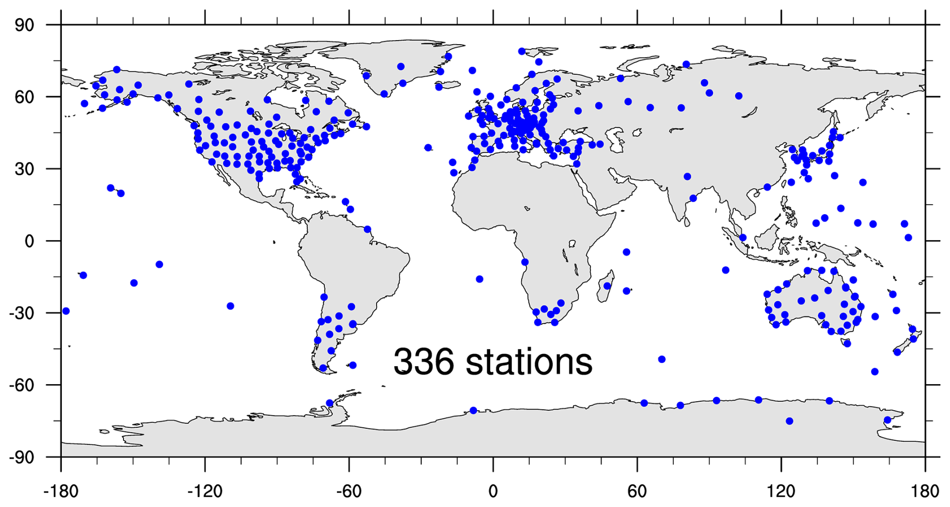
Figure 1 Locations of radiosonde stations that provided HVRRD used in this study over a 10 year period (2015–2024).

As described in detail in Ko et al. (2024), the radiosonde data used in this study underwent radiation correction and smoothing procedures (Ingleby et al., 2016). Although radiation corrections have been addressed in several studies (e.g., von Rohden et al., 2022; Lee et al., 2022b), the smoothing algorithms remain proprietary to the instrument manufacturers and are not publicly disclosed (Wang and Geller, 2025). Notably, Wang and Geller (2025) reported that temperature fluctuations in processed data can be reduced by up to a factor of two compared to raw data, with variations depending on the radiosonde instruments. These reduced small-scale temperature fluctuations in processed data may influence the estimation of vertical gradients used in Ri and ε calculations. In particular, reduced temperature variability may result in larger Ri values (i.e., more stable conditions) and consequently smaller ε estimates compared to calculations based on raw, unsmoothed data. Further assessment using raw radiosonde datasets would be valuable in future work. During the study period (2015–2024), a total of 25 radiosonde instrument types were identified across the globe. These include Beijing Changfeng CF-06, Graw DFM-17, Graw G., Graw M60, iMet-1-AB, iMet-2, iMet-4, iMet-54, Jin Yang RSG-20A, Lockheed Martin LMS-6, MARL-A, Meisei iMS-100, Meisei RS-11G, Meteolabor SRS-C34, Meteolabor SRS-C50, Meteosis MTS-01, Modem GPSonde M10, Modem M20, Polus-MRZ-N1, Vaisala RS41, Vaisala RS90, Vaisala RS92, Vaisala RS92-NGP, Vinohrady, and WEATHEX WxR-301D.

The HVRRD employed in this study have time resolutions of 1 and 2 s, but the vertical resolution is not uniform due to variations in the ascent rate of the radiosondes. To ensure consistency in vertical spacing, the 1 and 2 s resolution data were interpolated to 5 and 10 m intervals, respectively (Ko et al., 2024). The radiosonde dataset does not provide geometric height; only geopotential height is available. Therefore, the interpolation to uniform vertical spacing was performed with respect to geopotential height. Pressure and all other variables were interpolated consistently onto the same geopotential-height grid.

Instrumental noise can affect the potential temperature, resulting in regions of spurious N²<0 (Wilson et al., 2010, 2011). In addition, pendulum motion can affect wind observations (Faber et al., 2019). Pendulum period $\mathit{\omega }=\mathrm{2}\mathit{\pi }\sqrt{l/g}$ is determined by the balloon-payload (radiosonde) distance l and the gravitational acceleration g. Generally, the operational radiosondes are hung 30 m below the balloon (Faber et al., 2019), which corresponds to approximately 11 s of ω. Therefore, this study applied a moving average to temperature, pressure, zonal wind, and meridional wind, using a 13-point window for 1 s data and a 7-point window for 2 s data (both correspond to the 60 m vertical scale) to reduce instrumental noise and the effects of pendulum motion. The moving average is implemented as a centered scheme. At the top and bottom of the profile, where a complete window cannot be formed, the nearest valid averaged value is assigned to the edge levels to minimize boundary artifacts. Because the smoothing is applied after interpolation to uniform vertical spacing (5 m for 1 s data and 10 m for 2 s data), the effective vertical span corresponds to 60 m in both datasets. Turbulence layers thinner than 60 m, while potentially present in the atmosphere, especially thinner shear-driven turbulence, cannot be detectable with the current observational configuration. Due to the application of a 60 m moving average, all results will be presented only in cases where the thickness of the turbulence layer equals or greater than 60 m.

3.2 In-situ flight EDR (flight-EDR) data

As a validation of the newly suggested turbulence estimation in this study, flight-EDR (eddy dissipation rate; $\text{EDR}={\mathit{\epsilon }}^{\mathrm{1}/\mathrm{3}}$) observations obtained from commercial aircraft are used. EDR is a standard aviation turbulence metric and aircraft-independent measure of atmospheric turbulence (ICAO, 2010; Sharman et al., 2014). The flight-EDR data are derived using a vertical wind-based turbulence estimation algorithm, as aircraft are more sensitive to vertical gusts than horizontal ones (Hoblit, 1988; Sharman et al., 2014). Several types of reporting strategies are employed: 15 min routine reports, which are reported at regular intervals, and “triggered” reports, which are reported when the estimated EDR exceeds a preset threshold (0.18 ${\mathrm{m}}^{\mathrm{2}/\mathrm{3}}{\mathrm{s}}^{-\mathrm{1}}$). Additionally, some aircrafts generate 1 min routine reports, although these may include interpolated null values. However, the dataset used here does not indicate whether a report was interpolated or not. Therefore, all available reports are used without filtering. For consistency with the HVRRD-derived turbulence – which are only available when turbulence is present – we retain only those flight-EDR reports with EDR values greater than 0 ${\mathrm{m}}^{\mathrm{2}/\mathrm{3}}{\mathrm{s}}^{-\mathrm{1}}$. Further details regarding the turbulence estimation algorithm and reporting protocols can be found in Sharman et al. (2014).

3.3 ERA5 reanalysis pressure-level data

The ERA5 reanalysis dataset (Hersbach et al., 2020) provides hourly outputs with a horizontal resolution of 0.25°×0.25° (longitude × latitude) and 37 pressure levels spanning from 1000 to 1 hPa. The variables employed from ERA5 are zonal wind (u), meridional wind (v), and geopotential height (z). These fields are utilized in Sect. 4.2 to examine the large-scale flow associated with turbulence events.

4 Validation of Ri_min-based turbulence estimated from HVRRD

4.1 A case study

To evaluate the validity of the proposed method, a case study was first examined in Fig. 2. As shown in Fig. 2g, the Ri_min method identifies all three turbulence layers with Ri<0 (red) that are also captured by the Thorpe method in Fig. 2d. It additionally detects multiple turbulence layers with $\mathrm{0}<\mathit{\text{Ri}}<\mathrm{0.25}$ (blue), which are not detected by the Thorpe method. These newly identified layers correspond to regions of strong vertical wind shear in Fig. 2d. In Fig. 2e, two thin layers with $\mathrm{0}<\mathit{\text{Ri}}<\mathrm{0.25}$ are observed near z=10 and 11 km. However, these layers were excluded from Fig. 2g because their thicknesses were less than 60 m.

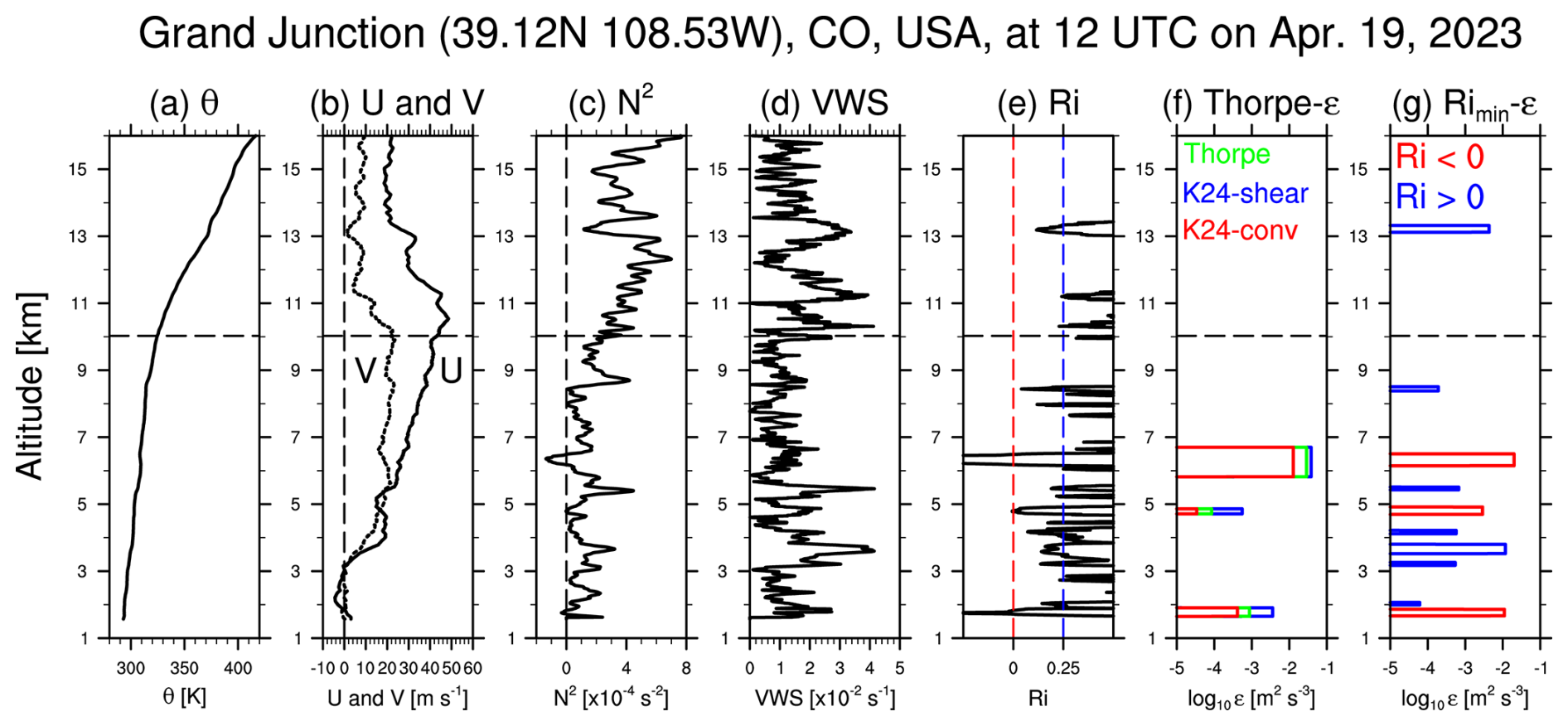
Figure 2 Vertical profiles observed at Grand Junction station (39.12° N, 108.53° W), CO, USA, at 12:00 UTC on 19 April 2023: (a) potential temperature, (b) zonal and meridional winds, (c) squared Brunt-Väisälä frequency, (d) vertical wind shear, (e) Richardson number, (f) Thorpe-estimated ε, and (g) Ri_min-based ε. In (f), green, blue, and red represent ε estimated using the conventional Thorpe method, the shear-driven assumption, and the convection-driven assumption based on Kantha (2024), respectively. In (g), red and blue indicate ε for negative and positive Ri cases, respectively. The horizontal dashed line in each plot denotes the tropopause height.

On the day of the observed case, clear and sunny weather conditions were reported, supporting the assumption that shear-driven turbulence is the dominant type. Therefore, in Fig. 2f, ε derived under the shear-driven assumption (blue) may to be the most reasonable assumption among the three turbulence estimates. Notably, ε values obtained from the Ri_min method in Fig. 2g are consistent in magnitude with those based on the shear-driven assumption in Fig. 2f. This agreement indicates that the proposed method not only broadens the turbulence detection but also yields ε values that are in quantitative agreement with the results from the Thorpe method under the reasonable assumption.

Meanwhile, as shown in Fig. 2g, the thickness of the turbulence layer estimated using the Ri_min method is generally thinner than that derived from the Thorpe method shown in Fig. 2f. This difference arises because the Ri_min method considers only regions where Ri is less than 0.25 as turbulence layers, unlike the Thorpe method which inherently overestimates the turbulence layers by including not only the observed overturning layers but also the surrounding statically stable regions required to restore stability (Thorpe, 1977). A climatological comparison with previously reported thicknesses distributions derived using the Thorpe method is provided in Fig. 6.

4.2 Comparison with flight-EDR data

To further illustrate the capability of the Ri_min method in detecting shear-driven turbulence under statically stable conditions ($\mathrm{0}<\mathit{\text{Ri}}<\mathrm{0.25}$), we additionally examined a representative jet-stream case (Fig. 3). The selected event occurred at 00:00 UTC on 13 January 2024, when a pronounced trough extended across the United States at 200 hPa, accompanied by a strong and curved jet stream on the southeastern flank of the trough. Such a synoptic configuration is dynamically favorable for enhanced vertical wind shear and Kelvin–Helmholtz instability in the statically stable upper troposphere. A zoomed-in view of the jet region (z=10–12 km) shows collocated HVRRD-derived Ri_min-based turbulence (circles) and flight-EDR reports (triangles), with colors indicating turbulence intensity categories following the definition of Sharman and Pearson (2017). In the region highlighted by the red box, both datasets consistently indicate severe-intensity turbulence in close spatial proximity, demonstrating that the Ri_min method successfully captures strong turbulence embedded within the high-shear jet environment. Conversely, in the two regions marked by yellow boxes, both datasets indicate null turbulence intensity, supporting the spatial consistency between the Ri_min-based estimates and aircraft observations. Although exact point-to-point collocation is inherently limited by differences in sampling strategy, the coherent spatial correspondence relative to the jet core provides qualitative yet physically meaningful support for the ability of the Ri_min method to detect shear-driven turbulence that may not involve overturning signatures identifiable by the Thorpe method.

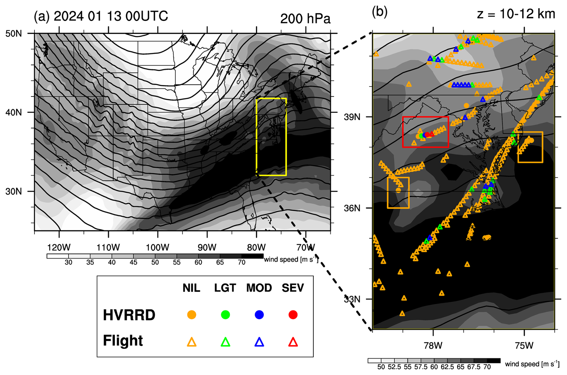
Figure 3 (a) Horizontal distribution of 200 hPa wind speed (shaded) and geopotential height (contours) at 00:00 UTC on 13 January 2024. (b) Zoomed-in view of wind speed at 200 hPa with overlaid turbulence observations at z=10–12 km. Filled circles and open triangles denote the turbulence estimated from HVRRD-Ri_min and that observed from in-situ flight-EDR, respectively. Colors represent turbulence intensity categories (null; NIL, light; LGT, moderate; MOD, and severe; SEV). The red box highlights a region where both datasets consistently indicate SEV turbulence in close proximity, while the yellow boxes mark regions where both datasets indicate NIL turbulence.

As an additional validation, this study examined the monthly time series of the ratio of moderate-or-greater (MOG) intensity turbulence events, defined as EDR≥0.22 ${\mathrm{m}}^{\mathrm{2}/\mathrm{3}}{\mathrm{s}}^{-\mathrm{1}}$ (Sharman and Pearson, 2017). Following Ko et al. (2023), who compared flight-EDR reports with HVRRD-EDR estimated using the Thorpe method over major U.S. routes, this study applied the same framework using the Ri_min-based method, alongside the Thorpe method for comparison. Specifically, major flight routes with dense flight-EDR reports were identified, then HVRRD-EDR were computed from HVRRD profiles collected at radiosonde stations located within those main flight routes (see Fig. S1 in the Supplement). Considering that HVRRD are available at 00:00 and 12:00 UTC, only flight-EDR reports observed within ±1 h of those times were used.

Figure 4 compares the monthly MOG ratios derived from flight-EDR and those of HVRRD-EDR derived from the Ri_min method and the Thorpe methods. The flight-EDR shows seasonal peaks (up to 2.5 %) in late winter and early spring, likely linked to enhanced jet activity and wind shear (Sharman et al., 2014). The Ri_min method captures this seasonality well, showing a strong and statistically significant correlation with flight-EDR (r=0.76). In contrast, the conventional Thorpe method shows almost no correlation ($r=-\mathrm{0.03}$), indicating poor performance in representing MOG variability revealed in aircraft measurements. The Thorpe method under the shear-driven assumption (K24-shear; green) improves the correlation (r=0.38), though still underperforms relative to the Ri_min method. The Thorpe method under the convection-driven assumption (K24-conv; orange) persistently underestimates MOG ratios (below 0.5 %) and shows a negative, insignificant correlation ($r=-\mathrm{0.15}$), likely due to its mismatch with the clear-air turbulence (CAT) nature of flight-EDR observations (Sharman et al., 2014; Ko et al., 2023). These results indicate that the Ri_min method more effectively captures the climatological variability of MOG intensity turbulence than the Thorpe method.

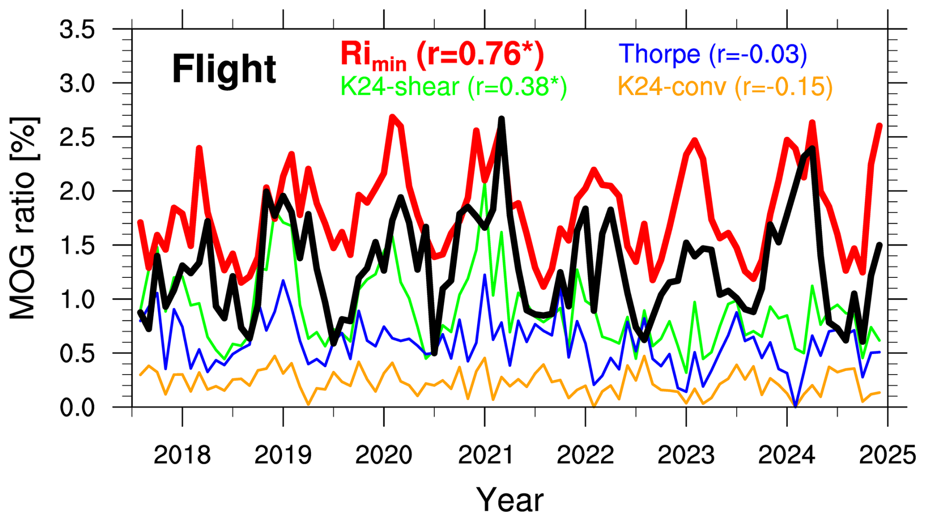
Figure 4 Time series of the monthly moderate-or-greater (MOG) intensity ratio for flight-EDR (black), Ri_min-EDR (red), and EDR estimated using the conventional Thorpe method (blue), the shear-driven assumption (green), and the convection-driven assumption (orange) based on Kantha (2024). The data cover the period from August 2017 to December 2024 (89 months) at z=20–40 kft within the main flight routes in the United States. “r” denotes the correlation coefficient between the MOG ratios of each EDR and flight-EDR, with * indicating statistical significance at the 99 % confidence level.

5 Global distributions of the Ri_min-based turbulence

This study further investigated the global distributions of Ri_min-based turbulence using HVRRD (2015–2024). Figure 5 presents seasonal occurrence frequency distributions of log ₁₀ε, defined as the number of turbulence events per bin normalized by the total number of HVRRD profiles in each domain. The panels distinguish between the Northern Hemisphere (NH) and Southern Hemisphere (SH), and between the troposphere (surface to tropopause) and stratosphere (tropopause to 30 km). Tropopause height was calculated for each profile using the WMO (1957) definition of the first tropopause. For each panel, log ₁₀ε distributions are shown separately for positive and negative Ri cases.

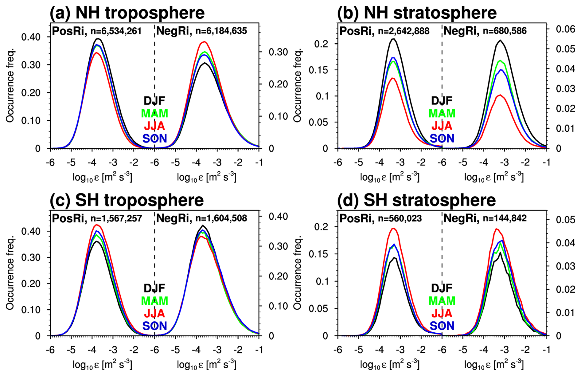
Figure 5 Occurrence frequencies of log ₁₀ε in (a) the Northern Hemisphere (NH) troposphere, (b) the NH stratosphere, (c) the Southern Hemisphere (SH) troposphere, and (d) the SH stratosphere over a 10 year period (2015–2024). In each plot, the left and right sides represent the results for positive Ri (PosRi) and negative Ri (NegRi) cases, respectively. The black, green, red, and blue lines indicate the results for December–January–February (DJF), March–April–May (MAM), June–July–August (JJA), and September–October–November (SON), respectively. “n” denotes the total occurrence number of log ₁₀ε in each domain.

Across all domains, log ₁₀ε ranges from −6 to −1 m² s⁻³, with peaks for positive Ri cases near −4. Negative Ri cases are slightly right-shifted, particularly in the troposphere, indicating that stronger turbulence is likely associated with convective overturning. In the stratosphere, negative Ri cases are less frequent but reach higher log ₁₀ε values than positive Ri cases, suggesting that while overturning is less likely to occur than non-overturning turbulence in the statically stable stratosphere, the intensity of turbulence that overcomes such strong stability and develops into overturning is greater than that of turbulence in positive Ri cases. The global mean of log ₁₀ε is −3.37 m² s⁻³, (−3.46 for positive Ri; −3.35 for negative Ri), consistent with previous studies based on the Thorpe method (Clayson and Kantha, 2008; Ko et al., 2024), aircraft (Sharman et al., 2014), and radar (Li et al., 2016) observations.

The positive Ri regime exhibits a clear seasonal cycle, with higher occurrences in winter (DJF in the NH, JJA in the SH) and lower in summer (JJA in the NH, DJF in the SH), reflecting enhanced shear-driven turbulence due to strong upper tropospheric and lower stratospheric (UTLS) jets (Koch et al., 2006). In the troposphere (Fig. 5a and c), negative Ri cases are most frequent during summer and least frequent in winter in both hemispheres, supporting the interpretation that turbulence in this regime is predominantly convectively generated. In contrast, stratospheric negative Ri cases (Fig. 5b and d) occur most frequently in winter in both hemispheres, suggesting that shear instability plays a dominant role in driving overturning turbulence in the stratosphere.

Figure 6 presents the occurrence frequency distributions of L, which characterizes the depth of mixing for momentum and trace gases and is a fundamental variable in turbulence modeling (Dewan, 1981; Osman et al., 2016; Muñoz-Esparza et al., 2020; Ko et al., 2024). Across all domains, the occurrence frequency of L exhibits an approximately exponential decay with increasing L. In the troposphere (Fig. 6a and c), negative Ri cases reach thicker layers (up to 1000 m) than positive Ri cases (up to 600 m), suggesting convectively generated turbulence extends deeper vertically than shear-driven turbulence. In the stratosphere (Fig. 6b and d), this contrast remains but is less pronounced, likely due to the stronger static stability that suppresses deep convective overturning.

Figure 6 The same as in Fig. 5, but for the thickness of the turbulence layer L.

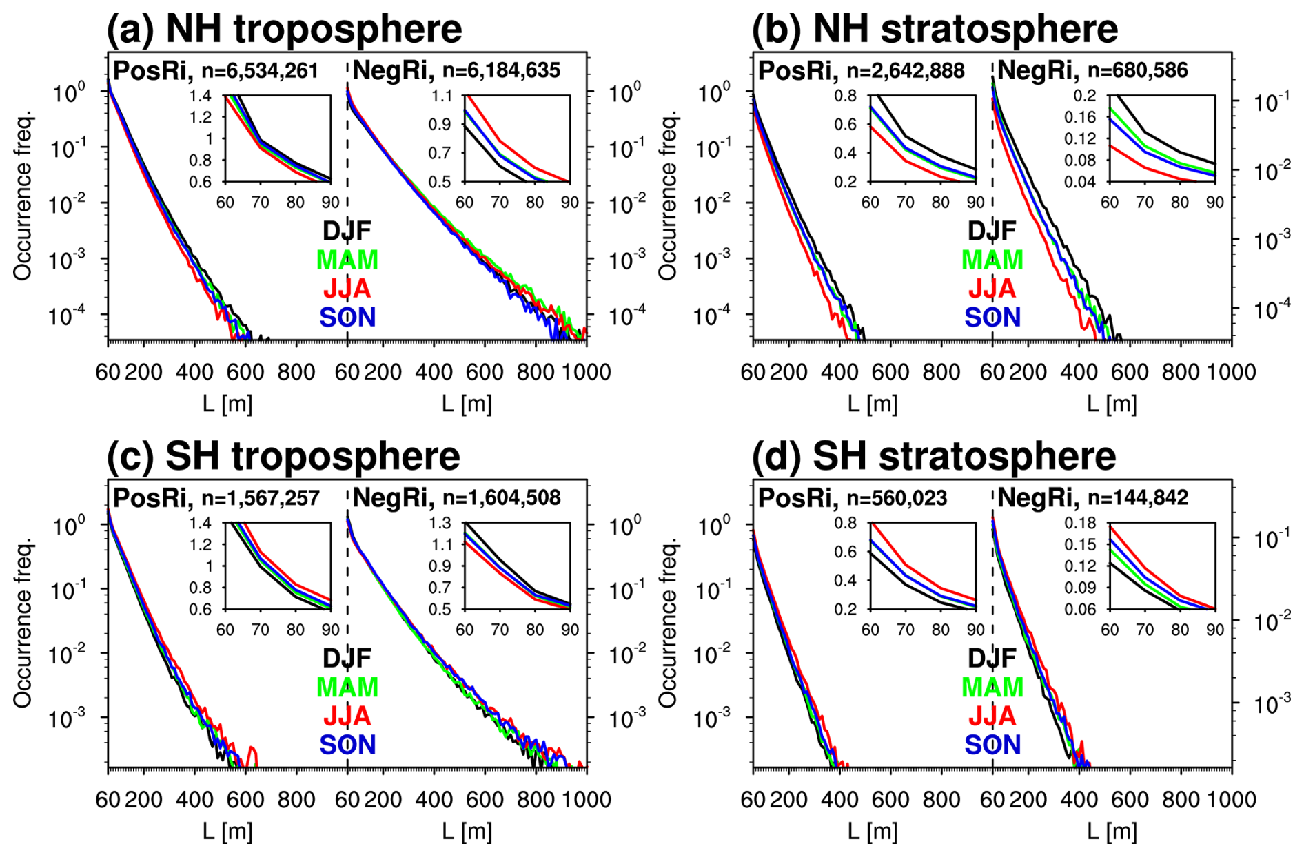
Globally, the 50th (median) and 95th percentiles of L are 90 and 225 m, respectively. These values are smaller than those reported by Ko et al. (2024). For positive Ri cases, the 50th and 95th percentiles are 80 and 180 m; for negative Ri cases, they are 100 and 270 m, reinforcing that overturning turbulence tends to produce thicker layers than those of positive Ri conditions. Seasonal variations in L are less prominent than those of log ₁₀ε (Fig. 5), so each panel includes a zoomed-in view up to the global 50th percentile (90 m) to better examine seasonal differences. The seasonal variations in L are consistent with those observed for log ₁₀ε. In the troposphere, positive Ri cases exhibit higher occurrence in winter, likely due to stronger jet-induced wind shear. A more quantitative assessment of the relationship between jet strength and turbulence occurrence frequency is provided later in Fig. 7. For negative Ri, a rightward shift in summer indicates deeper turbulence layers, consistent with enhanced convective activity during warmer months.

Figure 7 Vertical profiles of (a) horizontal wind speed and (b, c) nonzero turbulence frequency for positive and negative Ri cases, respectively, relative to the altitude of maximum wind speed (Z_WSPDmax) over a 10 year period (2015–2024). Blue and red lines represent the results for weak and strong jet-streams, respectively, as defined in the main text. Solid and dashed lines correspond to winter (DJF in the NH and JJA in the SH) and summer (JJA in the NH and DJF in the SH), respectively.

To further examine the vertical distribution of turbulence and its relationship with wind speed, Fig. 7 presents vertical profiles of wind speed and turbulence occurrence frequency. The vertical axis is aligned relative to the altitude of maximum wind speed (Z_WSPDmax) to account for variations in jet core height across different atmospheric conditions and latitudes. Here, the jet strength and Z_WSPDmax are determined following Koch et al. (2006): the horizontal wind speed (WSPD) averaged over two pressure levels is defined by $\mathit{\alpha }\text{vel}\equiv \frac{\mathrm{1}}{p_{\mathrm{2}}-p_{\mathrm{1}}}{\int }_{p_{\mathrm{1}}}^{p_{\mathrm{2}}}(u^{\mathrm{2}}+v^{\mathrm{2}}{)}^{\mathrm{1}/\mathrm{2}}\mathrm{d}p$, where u and v are the zonal and meridional wind, respectively, and p₁ and p₂ are set to 400 and 100 hPa, respectively. Within this 400–100 hPa, the altitude at which the maximum WSPD is defined as Z_WSPDmax. Then, αvel≥30 m s⁻¹ and αvel<30 m s⁻¹ are classified as “strong jet condition” and “weak jet condition” cases, respectively. In Fig. 7a, by definition, strong jet conditions exhibit significantly higher wind speeds, with winter profiles (solid lines) being stronger and deeper than summer profiles (dashed lines).

Figure 7b and c show the occurrence frequency of turbulence derived from the Ri_min method, separated by positive and negative Ri regimes. In the positive Ri regime, two peaks appear: one near the upper-tropospheric jet core and another in the lower troposphere. Strong jets (red) show significantly higher turbulence frequencies than weak jets (blue), especially in the upper troposphere. Winter profiles (solid lines) exhibit consistently greater turbulence frequencies than summer profiles (dashed lines), reflecting enhanced wind shear environments favorable for turbulence generation. In the negative Ri regime (Fig. 7c), a dominant peak appears in the lower troposphere, where surface heating and convective activity are most pronounced. Jet strength has little influence at UTLS in this regime, as shown by minimal differences between strong and weak jet conditions. In contrast, seasonal variation is more pronounced in this negative Ri regime: turbulence is more frequent in summer than in winter, consistent with increased convective activity during warmer months.

Previous studies (Ko and Chun, 2022; Ko et al., 2024) have shown that a simple arithmetic mean of log ₁₀ε does not properly represent turbulence characteristics, particularly in the stratosphere where turbulence is infrequent and a few strong ε events can dominate the average. In contrast, the troposphere generally exhibits greater turbulence occurrence and thicker turbulence layers (see Fig. 6). To better characterize layer-averaged turbulence, this study adopts the effective ε (EE) introduced by Ko and Chun (2022), which integrates both the turbulence intensity (ε) and the vertical extent (L) of each turbulence layer. EE reflects the atmospheric portion affected by turbulence within a given altitude range, and is defined as $\text{EE}=\sum (\mathit{\epsilon }\times L)/Z$ in units of [m² s⁻³], where Z is the depth of the layer considered. In Fig. 8, Z is approximately 11.4 km in the troposphere and 18.3 km in the stratosphere, while in Fig. 9, Z is uniformly 1 km.

Figure 8 shows the global distribution of log ₁₀EE at individual radiosonde stations. Here, log ₁₀EE denotes log ₁₀(EE/1 m² s⁻³), ensuring that the logarithm is taken of a dimensionless quantity. The highest values appear in negative Ri cases within the troposphere (Fig. 8c), while the lowest values occur in the stratosphere for negative Ri regime (Fig. 8d). Positive Ri cases (Fig. 8a and b) yield similar log ₁₀EE values in both layers. These patterns indicate that turbulence associated with convective instability in the troposphere is stronger than that generated by shear-driven processes. In Fig. 8a, the distribution of log ₁₀EE for positive Ri cases in the troposphere shows intermediate values across most regions, with relatively higher values over Türkiye, the eastern U.S., Central Europe, East Asia, and the southern Andes. Lower values appear in the tropics and northern high latitudes. The stratospheric counterpart (Fig. 8b) exhibits a similar spatial pattern but with even lower at high latitudes of both hemispheres.

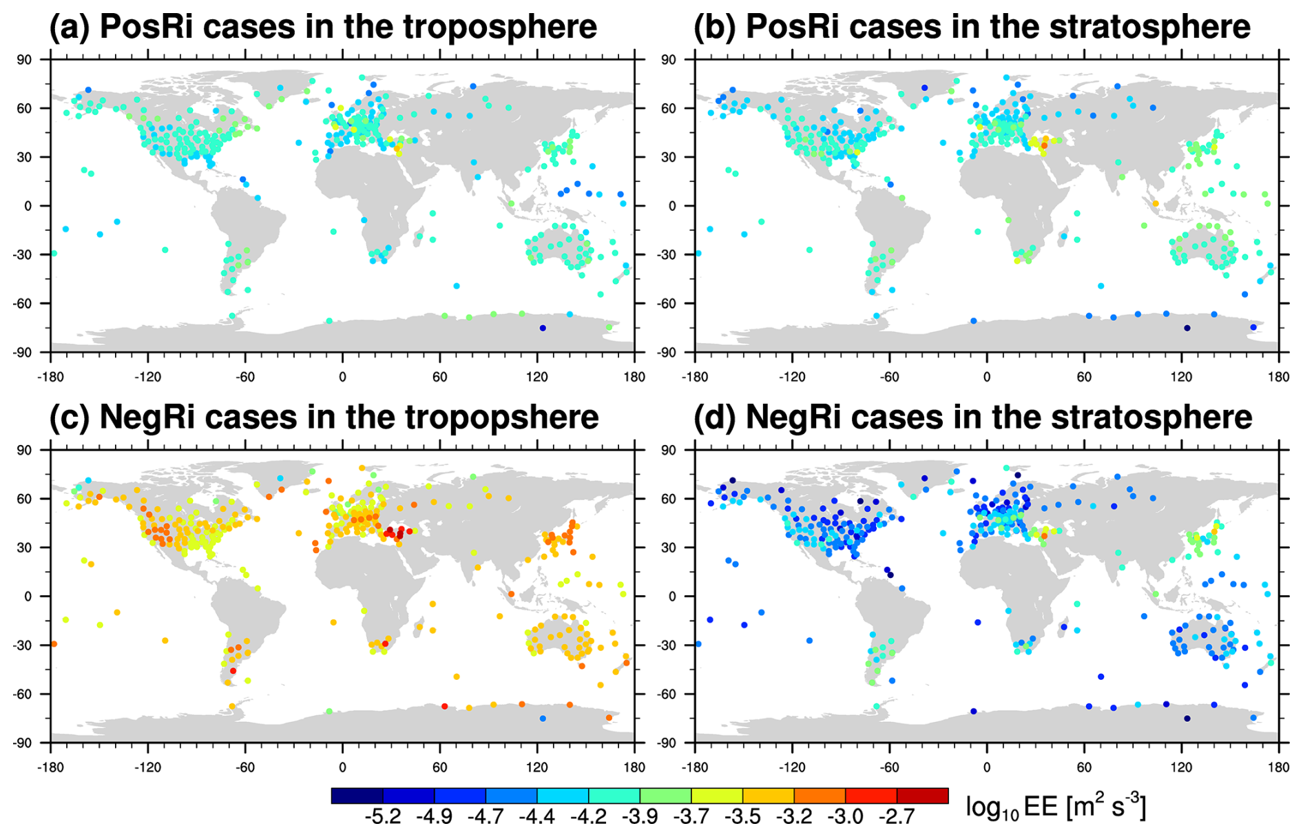
Figure 8 Global distributions of log ₁₀EE at each station over a 10 year period (2015–2024) for (a) positive Ri (PosRi) cases in the troposphere, (b) PosRi cases in the stratosphere, (c) negative Ri (NegRi) cases in the troposphere, and (d) NegRi cases in the the stratosphere.

In Fig. 8c, negative Ri cases in the troposphere show that log ₁₀EE values are strong over Türkiye, the western United States, East Asia, and South America. These regions have significant and complex terrain, suggesting that turbulence could originate from orographic sources such as orographically induced convection and the breaking of convective and mountain gravity waves. In contrast, stations in the tropics and polar regions show relatively lower values compared to the other regions. In Fig. 8d, the lowest log ₁₀EE values are revealed among the four domains, reflecting the rarity of negative Ri cases in the highly stratified stratosphere. Slightly elevated values are seen over Türkiye, East Asia, and South America, while lower values are observed over the eastern U.S., Northern Europe, Australia, and Antarctica. The spatial pattern of log ₁₀EE with negative Ri cases is consistent with that from the Thorpe method in Ko et al. (2024) in terms of the range of values, the maximum over Türkiye, and locally large values over East Asia and South America. This agreement likely stems from the conceptual similarity between both methods, which identify turbulence under statically unstable conditions (i.e., N²<0). Further regional analysis will be presented in Fig. 10.

Figure 9 presents the vertical distribution of log ₁₀EE in 1 km bins (i.e., Z=1 km) relative to the tropopause height z−z_tp to consider the latitudinal and seasonal variations in the tropopause (Birner, 2006). Here, z is the geometric altitude above mean sea level and z_tp is the tropopause height of each HVRRD profile.

For positive Ri cases, the global median log ₁₀EE exhibits a smooth profile with little contrast between the troposphere and stratosphere. Peak median values occur near the tropopause, indicating enhanced turbulence activity in this UTLS. In contrast, negative Ri cases show a distinct structure: log ₁₀EE peaks in the lower troposphere, where convective instability is more likely to occur due to surface heating and buoyancy, then decreases sharply with altitude. Comparing the two regimes of Ri, median log ₁₀EE is higher for negative Ri cases in the troposphere, whereas positive Ri cases dominate in the stratosphere – highlighting different turbulence generation mechanisms in the two regimes. Moreover, negative Ri cases exhibit a broader spread in log ₁₀EE across most altitudes, reflecting the more variable and intermittent nature of overturning turbulence. The vertical structure for negative Ri cases is consistent with the Thorpe method results in Ko et al. (2024), as in the horizontal distributions in Fig. 8.

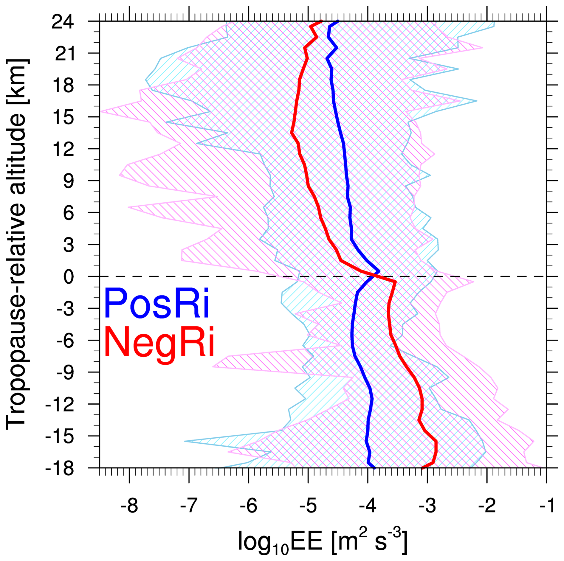
Figure 9 Vertical distributions of log ₁₀EE within each 1 km altitude bin relative to the tropopause over a 10 year period (2015–2024). Thick lines represent the median values of log ₁₀EE, while the hatched areas indicate the full range. Blue and red represent the results for positive and negative Ri cases, respectively.

To assess regional variability, Fig. 10 presents statistics of log ₁₀EE across 10 globally defined regions (Fig. 10a), determined based on geographical proximity and non-overlapping station coverage. Figure 10b and c show boxplots of log ₁₀EE for positive and negative Ri cases, respectively.

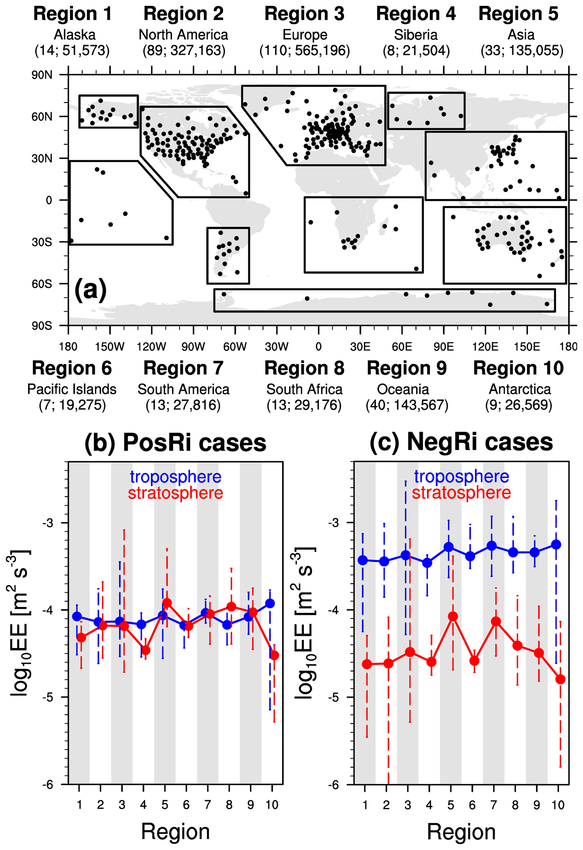
Figure 10 (a) Division of radiosonde stations into Regions 1–10, with the number of stations and profiles in each region over a 10 year period (2015–2024). (b, c) Median (dots) and full range (dashed lines) of log ₁₀EE in each region in the troposphere (blue) and stratosphere (red), shown separately for positive Ri (PosRi) and negative Ri (NegRi) cases.

For positive Ri cases (Fig. 10b), regional differences are relatively small both in the troposphere and the stratosphere. Tropospheric median values are uniform, with slightly elevated values in Regions 5 (Asia), 7 (South America), and 10 (Antarctica). Stratospheric medians are comparable with tropospheric medians, but show greater inter-regional variability as represented by wider dashed lines in the stratosphere than in the troposphere. A similar pattern is observed for negative Ri cases (Fig. 10c), consistent with Ko et al. (2024), likely due to broader horizontal drifting of radiosondes at higher altitudes. Tropospheric EE values for negative Ri are notably higher than those for positive Ri, again peaking in Regions 5, 7, and 10, reaffirming that turbulence is generally more vigorous and variable under unstable stratification than under stable conditions. In the stratosphere, by contrast, negative Ri cases exhibit considerably lower EE values than in the troposphere, primarily due to their rarity in the stratosphere.

Interestingly, both positive and negative Ri cases in the troposphere show the global maximum of median log ₁₀EE in Region 10 (Antarctica), contrasting with the stratospheric minimum over the same region. This also differs from Ko et al. (2024), where Antarctica showed the lowest EE in the troposphere. This discrepancy likely stems from different definitions of the troposphere: the present study includes all levels up to the tropopause, while Ko et al. (2024) exclusively considered in the free troposphere (3 km above the station to the tropopause). When our calculations are restricted to the free troposphere (Fig. S2), Antarctic values decreased substantially, aligning with Ko et al. (2024). This implies that EE values in the lower troposphere over Antarctica are particularly large, and these elevated values may reflect strong orographic effects. Yoo et al. (2020) showed that steep slopes near the Antarctic edge enhance frontogenesis, particularly at 850 hPa. Since most Antarctic HVRRD stations are located along these margins (Fig. 1), enhanced turbulence in this region may be influenced by orographic effects and associated dynamical processes. Additionally, under the free troposphere definition, the highest EE appears over Region 5 (Asia), consistent with Ko et al. (2024).

6 Data availability

The turbulence data obtained from the current study based on the Ri_min method using high vertical-resolution radiosonde data (HVRRD) Version 1.0 for 2015–2024 are available at https://doi.org/10.5281/zenodo.16899801 (Ko and Chun, 2025a), https://doi.org/10.5281/zenodo.16899803 (Ko and Chun, 2025b), https://doi.org/10.5281/zenodo.16899805 (Ko and Chun, 2025c), https://doi.org/10.5281/zenodo.16810246 (Ko and Chun, 2025d), and https://doi.org/10.5281/zenodo.16899789 (Ko and Chun, 2025e). The final archived dataset is provided in NetCDF (Network Common Data Form) format. A summary table listing all variables and their physical units is provided in Table S1 in the Supplement.

The HVRRD used in this study to estimate turbulence are openly available from the National Centers for Environmental Information (NCEI, 2025; https://www.ncei.noaa.gov/data/ecmwf-global-upper-air-bufr/). In-situ flight EDR data are available from the National Oceanic and Atmospheric Administration (NOAA)'s Meteorological Assimilation Data Ingest System (MADIS) site (NOAA MADIS, 2025; https://madis-data.cprk.ncep.noaa.gov/madisPublic1/data/archive/). ERA5 reanalysis datasets are openly available from the European Centre for Medium-Range Weather forecasts (ECMWF, 2020; https://doi.org/10.24381/cds.bd0915c6).

7 Summary and conclusions

By utilizing HVRRD to estimate atmospheric turbulence, this study introduced a new method based on Ri_min, addressing key limitations of the widely used Thorpe method. While the Thorpe method identifies turbulence associated with static instability (i.e., N²<0) exclusively, the Ri_min method can capture turbulence even under statically stable and strongly shear conditions ($\mathrm{0}<\mathit{\text{Ri}}<\mathrm{0.25}$). Comparisons with flight-EDR data showed that Ri_min method correlates significantly better with observed turbulence and outperforms the Thorpe method. Using 10 years (2015–2024) of global HVRRD, this study conducted a comprehensive climatological analysis of turbulence derived from the Ri_min method. Turbulence under positive Ri conditions peaked in winter and minimized in summer, consistent with seasonal variations in jet stream intensity. In contrast, negative Ri cases were more frequent in summer and less in winter in the troposphere, with the opposite seasonal variation in the stratosphere. To better represent layer-mean turbulence, this study employed the effective ε (EE), combining turbulence intensity (ε) with layer thickness (L). High EE values were found over Asia, southern America, and Antarctica, with Antarctic values largely driven by near-surface turbulence likely linked to strong topographic forcing. In the free atmosphere, EE was highest over Asia and lowest over Antarctica, consistent with previous findings.

As HVRRD inherently reflects the effects of turbulence, it is not well-suited for investigating the background atmospheric conditions responsible for turbulence generation (Ko and Chun, 2022) in the present study. To address this limitation of HVRRD, Ko and Chun (2022) used ERA5, the highest-resolution global reanalysis datasets currently available (Hersbach et al., 2020), to examine the potential sources of turbulence detected by the Thorpe method. Similar approach is required to investigate potential sources of turbulence detected in the present study, which remains for future research.

This study provides quantitative information on turbulence location and intensity, supporting validation of aviation turbulence forecasts. Currently, only the flight-EDR data have been used to validate the aviation turbulence forecasts, and these observations are concentrated along major flight routes and tend to avoid regions of strong convective activity, resulting in spatial sampling biases (Ko et al., 2023). Under this situation, turbulence estimated from HVRRD, such as from the current study, offers a complementary observational dataset, especially in regions where aircraft observations are limited or unavailable. Ultimately, this application has the potential to contribute to safer and more efficient flight operations.

Importantly, the present study used publicly available high-resolution radiosonde data provided by operational stations. As more radiosonde stations offer 1 or 2 s resolution data, future research on atmospheric turbulence will benefit from increased spatial coverage. It is highly imperative that high-resolution data be made available for international use, although some countries still do not provide HVRRD internationally (Ko et al., 2024). Broader data sharing of HVRRD will greatly benefit not only turbulence research but also studies on general atmospheric research, including gravity waves, boundary layer structure, tropopause dynamics, and numerical model validation.