Phytoplankton coastal-offshore monitoring by the Strait of Dover at high spatial resolution: the DYPHYRAD surveys

Long-term monitoring of phytoplankton communities is essential for understanding the functioning and evolution of marine systems. This paper presents a decadal dataset on phytoplankton observations conducted along a coastal-offshore transect by the Strait of Dover, at fine spatial resolution, using an automated in vivo approach. Nine stations (∼ 1 km apart) were sampled in the sub-surface off the Slack estuary, representing the northern limit of the Marine Protected Area of “Picard Estuaries and Opal Seas” (EPMO). Since 2012, phytoplankton functional groups were characterised in vivo in sub-surface waters using multi-spectral fluorometry (Fluoroprobe, bbe Moldaenke, Gmbh) and single-cell optical analysis with a pulse shape-recording flow cytometer (CytoSense and CytoSub, Cytobuoy b.v., the Netherlands). Total phytoplankton biomass was estimated via chlorophyll a extraction and in vivo fluorescence. Spectral and functional groups were quantified in terms of abundance, size, and estimated chlorophyll a in surface waters. Weekly sampling resolution allowed us to address the community composition in order to disentangle short-term, fine spatial, seasonal, and inter-annual variability. Additionally, biogeochemical and hydrological variables: temperature, salinity, Photosynthetically Active Radiation (PAR), and nutrients (nitrate, nitrite, phosphate, silicate) were systematically measured. Over 11 years, the survey generated 1835 samples from 268 dates, averaging 167 samples per year across 24 cruises. This unique dataset provides valuable insights into phytoplankton dynamics and environmental drivers in a temperate coastal system. Free access to the dataset can be found at https://doi.org/10.17882/104524 (Hubert et al., 2025b).

1 Introduction

Phytoplankton are central to marine ecosystems, driving much of the primary production (Rousseaux and Gregg, 2014) and forming the foundation of most marine food webs (Berglund et al., 2007; Falkowski and Raven, 2007). Their contribution to biogeochemical cycles, including their role in climate regulation through the biological pump, makes them a critical component of oceanic systems (Giering and Humphreys, 2017). As their dynamics are closely linked to environmental variations, phytoplankton are increasingly used as biological indicators for assessing marine ecosystem health (Bierman et al., 2011; Rombouts et al., 2019). Understanding these dynamics is particularly important in regions subject to significant anthropogenic pressures and environmental variability, such as Pas-de-Calais (Strait of Dover). The Strait of Dover, which connects the English Channel and the North Sea, is characterised by intense maritime activity (Wang et al., 2023), heavy fishing pressure (Girardin et al., 2015), and the influence of adjacent industrialised areas (e.g., ports, industrial activities) and agricultural regions, as well as runoff from local estuaries. The hydrodynamic regime characterised by strong currents, a macro-tidal regime as well as remote and local estuarine inputs significantly shape phytoplankton communities in this region (Desmit et al., 2020; Kang et al., 2021; Salmaso and Tolotti, 2021). This area is also subject to regular blooms of Phaeocystis globosa Scherffel (Astoreca et al., 2009; Lefebvre et al., 2011; Breton et al., 2022; Skouroliakou et al., 2022, 2024), a haptophyte species whose genus is known for its wide distribution and potential ecological impact (Smith and Trimborn, 2024). While non-toxic in the Eastern English Channel and the North Sea (Cadée and Hegeman, 2002), they are classified as harmful algae blooms (HAB) by UNESCO (Lundholm et al., 2025) because these blooms are considered undesirable due to their tendency to form dense gelatinous colonies and foam layers, particularly during periods of strong winds (Lefebvre and Delpech, 2004). This phenomenon affects water density, potentially disrupts both benthic and pelagic ecosystems (Karasiewicz et al., 2018), and has occasionally resulted in human fatalities (Peperzak and van Wezel, 2023).

Historically, phytoplankton monitoring in this region has been conducted within French National Observation Services (SNO) through long-standing networks such as SRN-REPHY (https://manchemerdunord.ifremer.fr/Environnement/LER-Boulogne-sur-Mer/Surveillance-et-Observation/Reseaux-nationaux, last access: 6 March 2025), SOMLIT (https://www.somlit.fr/wimereux/, last access: 6 March 2025), and PhytOBS (https://www.phytobs.fr/Stations/Boulogne, last access: 6 March 2025), providing valuable and accessible data on chlorophyll a concentration and microphytoplankton diversity. However, these programs are set for monthly to fortnightly collection on a reduced number of stations, and consider mainly microscopic counts of micro- and some nanophytoplankton species, even though, since 2009, pico- and nanoplankton abundance were addressed by benchtop flow cytometry on fixed samples at some stations. Advances in automated monitoring technologies enable more detailed observations of phytoplankton communities, providing insights across the entire size spectrum from a single in vivo sample and allowing data acquisition at higher spatial and temporal resolutions. This study presents the DYnamics of PHYtoplankton on RADiale (DYPHYRAD) of the Saint-Jean Bay dataset, encompassing 11 years (2012–2022) of automated, high-resolution monitoring of phytoplankton communities on a coastal-offshore transect in the Strait of Dover. Weekly surveys were conducted along a coastal-offshore transect, integrating data from a multi-spectral fluorometer (Fluoroprobe, bbe Moldaenke, Gmbh) and an automated pulse-shape recording flow cytometer (CytoSense and CytoSub, Cytobuoy b.v., the Netherlands). Combined with hydrological and biogeochemical measurements, this dataset provides a comprehensive view of phytoplankton dynamics (including abundance, scatter, fluorescence, chlorophyll a and pigments content) at a fine spatial scale. By making this dataset available in accordance with FAIR principles (Findable, Accessible, Interoperable, Reusable), this research aims to support further studies on seasonal and inter-annual variations, long-term trends, and the impacts of environmental drivers on phytoplankton communities. In doing so, it offers valuable contributions to understanding the health and resilience of marine coastal ecosystems under increasing anthropogenic and climate pressures.

2 Aim of the data collection

Long-term observation data are essential for understanding the functioning and state of marine ecosystems and for providing environmental managers with the information needed to mitigate anthropogenic pressures on marine ecosystems. By integrating these data into public policy indicators of ocean health and biodiversity, effective measures can be devised to preserve marine environments. The DYPHYRAD surveys focus on understanding the dynamics of marine phytoplankton and their associated environmental variables across the distinct water masses of the Strait of Dover. These measurements complement national and regional monitoring networks (SOMLIT, REPHY, PhytOBS) by providing higher sampling frequency (weekly) and finer spatial resolution (∼ kilometer scale). Since 2022, this monitoring program has been recognised as an observation of interest for the French research and manager's community of the national Coastal and Littoral French Research Infrastructure (ILICO, i.e. Infrastructure de recherche LIttorale et CÔtière).

3 Material and Methods

3.1 Study site

The Eastern English Channel (EEC) is a shallow region, with depths not exceeding 50 m, and is influenced by a macro- and mega-tidal regime that can exceed 8 m. These tidal forces, combined with the area's bathymetry, variable wind regimes, and proximity to the Pas-de-Calais (Strait of Dover), generate strong hydrodynamics, with average current velocities reaching 1 m s⁻¹ (Lazure and Desmare, 2012; Thiébaut and Sentchev, 2016). The predominant drift of these currents towards the Northeast intensifies mixing and stratification processes within the water column, significantly affecting the physico-chemical characteristics of the region (e.g., mixing/stratification) (Lazure and Desmare, 2012). Coastal waters in the EEC are further enriched by nutrient inputs from numerous watersheds, including the Somme, Authie, Canche, Liane, Wimereux, and Slack estuaries along the Picardy and Opale coasts (Bentley et al., 1993). These influences lead to the formation of a Region of Freshwater Influence (ROFI), where freshwater outflows from these estuaries create a distinct coastal water mass that remains along the coast, separated from the offshore waters by a tidal front (Brylinski et al., 1991). This “coastal flow” presents unique characteristics and interacts dynamically with adjacent water masses.

The DYPHYRAD transect is strategically located in this complex environment, near the Strait of Dover, at the northern edge of the Picardy Estuaries and Opal Sea Marine Protected Area (EPMO). Positioned off the Slack estuary, the transect captures the combined influence of several estuaries within the EPMO (Fig. 1). By extending from the offshore to the coast, the transect allows for monitoring, at high spatial resolution, water bodies that are often very close but have distinct properties. This location is crucial for long-term monitoring, as it allows for the study of cumulative estuarine effects and the interactions between coastal and offshore water masses. The DYPHYRAD monitoring offers weekly observations that enhance our understanding of the hydrodynamics and environmental variability in this ecologically and economically important region.

3.2 Sampling strategy

From 2012 to 2022, weekly sampling and measurements were conducted along a sub-surface (1 to 2 m depth) coastal-offshore transect by the Strait of Dover aboard the research vessel “Sepia II” (CNRS INSU, French Oceanography Fleet-FOF). While the goal was to maintain a regular weekly sampling schedule, the actual frequency was occasionally disrupted by adverse weather conditions (e.g., during the winter of 2015), unexpected logistical issues, and the COVID-19 pandemic, including a prolonged interruption during the lockdown in the spring of 2020. Details on the frequency of cruises and the number of stations sampled are summarised in Fig. 2. Seasons are defined as winter (December–January–Ferbuary), spring (March–April–May), summer (June–July–August) and fall (September–October–November). The transect spans 9.7 km, consisting of nine sub-surface (1–2 m) sampling stations from R4 (50°8^′ N, 1°45^′22 E) offshore to R0 (50°8^′ N, 1°59^′ E) nearshore (Fig. 1; Table A1 in Appendix A). The coordinates of the sampling stations are detailed in Table A1. This transect captures key environmental gradients, such as those driven by estuarine inputs and hydrodynamic mixing. High-resolution hydrological measurements, including temperature, salinity, Photosynthetically Active Radiation (PAR), in vivo chlorophyll a fluorescence, and turbidity, were collected throughout the water column at each station using a multi-parameter CTD probe. Seawater samples were collected using Niskin bottles at approximately 1.5 m from the surface. Dissolved inorganic nutrients (nitrite, nitrate, phosphate, silicate) were measured from surface water samples at the main stations R0, R1, R2, R3, and R4. Discrete samples were used to measure biological variables, including in vivo chlorophyll a fluorescence, extracted chlorophyll a, and phaeopigments. Phytoplankton spectral and functional diversity was assessed at all nine stations using a combination of optical and fluorometric approaches on surface in vivo samples. Between 2018 and 2020, extra daily sampling cruises were conducted at three key stations (R1, R2, and R4) to capture high-frequency dynamics during periods of particular interest in June–July and September–October in order to capture rapidly changing phytoplankton dynamics. The post-bloom period was chosen because of the high bacterial activity following Phaeocystis globosa Scheffrel blooms (Lamy et al., 2009) and sporadic low-intensity blooms may occur in autumn (Breton et al., 2000). These additional surveys supported a range of analyses, including phytoplankton microscopy and molecular characterisation of microbial diversity through metabarcoding techniques (Fig. 2; Skouroliakou et al., 2022, 2024).

Figure 1 Map of the study area (indicated by the red square on the high scale map) and location of DYPHYRAD stations. The bathymetry data come from SHOM 2015 and 2016 (https://diffusion.shom.fr/donnees/bathymerie/mnt-cotier-pas-de-calais.html, last access: 28 January 2026).

Figure 2 Distribution of DYPHYRAD sampling over years (2012–2022). The dot size represents the number of monitored stations for each discrete sampling.

3.3 Hydrological and biogeochemical variables

Depth, temperature, salinity, PAR, and fluorescence were measured across the water column at each sampling point using a CTD profiler (SBE 19+ and SBE 25, SeaBird Ltd, United States) equipped with a WETStar Fluorometer (SeaBird Ltd, United States). Sub-surface values were calculated as the average of measurements taken between 1 and 2 m deep, ensuring consistency with the depth at which discrete water samples were collected. Additional measurements of temperature and conductivity/salinity were acquired by a manual probe on the surface and, since 2017, a thermo-salinograph (TSG) installed on the research vessel “Sepia II”, which continuously samples seawater at approximately 2.5 m deep via an onboard pump. While only CTD-derived data are presented in this study due to their coverage of the full study period, manual probe and TSG data are available for complementary analyses.

Concentrations of dissolved inorganic nutrients NO${}_{\mathrm{2}}^{-}$, NO${}_{\mathrm{3}}^{-}$, SiO₂ and H₃PO₄) were collected at the sub-surface using Niskin bottles. The samples were transferred to sterile 50 mL PVC flasks without pre-filtration and were analysed on the day of collection or frozen at −20 °C following the guidelines of Aminot and Kérouel (2007). The concentrations of nutrients were quantified using an autoanalyzer (AutoAnalyzer ALLIANCE SpA, Italy, then, since 2016, AA3 HR AutoAnalyzer, SEAL Analytical GmBH, Germany). The analyses followed the SOMLIT protocol, based on the methodology described by Aminot and Kérouel (2007), and were performed on single (non-replicated) samples.

In the laboratory, water samples for chlorophyll a and phaeopigment analyses were kept in the dark inside a cooler, then were filtered onto GF/C 47 mm Whatman glass fiber filters and stored at −80 °C until processing. Pigments were extracted in vitro using 90 % acetone. Filters were ground, refrigerated at 4 °C overnight, and analysed using a Turner Designs benchtop fluorometer (10-AU Field Fluorometer, Turner Designs Ltd., United States). Fluorescence emission at 685 nm was measured after excitation at 440 nm, both before and after acidification with 0.3 mol L⁻¹ HCl, following the protocol of Holm-Hansen et al. (1965). Chlorophyll a and phaeopigment concentrations were estimated using the equations of Lorenzen (1967). The percentage of chlorophyll a relative to total pigments was calculated, providing a proxy for the proportion of active pigments. Calibration of the fluorometer with pure chlorophyll a was performed annually to ensure measurement accuracy.

3.4 Automated in vivo phytoplankton measurements

Automated optical instruments were used to characterise phytoplankton at complementary levels of organisation. Mono-spectral in vivo fluorometry provided estimates of total chlorophyll a. Multi-spectral fluorometry resolved major pigmentary groups based on their distinct excitation–emission signatures. Automated flow cytometry quantified the abundance of phytoplankton functional groups by detecting single-cell optical properties. Together, these approaches offered a coherent and multi-dimensional description of phytoplankton biomass and composition over the study period.

The phytoplankton community in the EEC shows strong seasonal succession. Diatoms generally dominate most of the year, representing up to 85 % of total phytoplankton biomass (Breton et al., 2000; Grattepanche et al., 2011; Lefebvre et al., 2011; Hernandez-Farinas et al., 2014), except during the spring bloom when the Prymnesiophyte Phaeocystis globosa Scheffrel can exceed 90 % of biomass (Brunet et al., 1996; Lamy et al., 2009; Guiselin, 2010; Bonato et al., 2016). Pre- and post-bloom periods are marked by two distinct diatom blooms observed via microscopy, HPLC pigment analysis, multispectral fluorimetry, automated flow cytometry, and environmental DNA (Breton et al., 2000; Schapira et al., 2008; Guiselin, 2010; Monchy et al., 2012; Houliez et al., 2013; Christaki et al., 2014; Bonato et al., 2016). Cyanobacteria, picoeukaryotes, and Phaeocystis globosa Scheffrel dominate abundance patterns, with Synechococcus spp. and picoeukaryotes prevailing in winter and summer, while cryptophytes, coccolithophores, and dinoflagellates occur at lower abundances (Hernandez-Farinas et al., 2014; Bonato et al., 2016). Phytoplankton biomass and abundance are influenced by environmental conditions, hydrodynamics, grazing pressure, and microbial seasonal dynamics (Cotonnec et al., 2001; Seuront, 2005; Lamy et al., 2009; Rachik et al., 2018).

3.4.1 Total chlorophyll a estimated by in vivo mono-spectral fluorometry

Upon returning to the laboratory, after a maximum of 4 h of dark conservation in a cooler, in vivo fluorescence was measured immediately on 50 mL water samples using a Turner Designs benchtop fluorometer (10-AU Field Fluorometer, Turner Designs Ltd, USA). Measurements captured the maximum, minimum, and stabilised mean fluorescence at 685 nm following excitation at 440 nm, which provided an estimate of total chlorophyll a fluorescence. Checking instrument stability was performed using a dedicated solid standard to ensure measurement accuracy and reliability.

3.4.2 Phytoplankton spectral (pigmentary) groups addressed by in vivo multi-spectral fluorometry

In the laboratory, each sample kept in the dark in a cooler, was analysed within maximum 4 h of collection using a multi-spectral fluorometer (FluoroProbe, FLP, bbe Moldaenke, GmbH). The FluoroProbe emits light at five wavelengths (470, 525, 570, 590 and 610 nm) to differentiate among four phytoplankton pigmentary groups (Fig. 3) and at 370 nm (UV LED) to correct for fluorescence contributions from yellow substances. Operated in benchtop mode, the instrument estimates the concentration or relative contribution up to five phytoplankton pigmentary groups in total chlorophyll a equivalents (µg chl-a eq. L⁻¹).

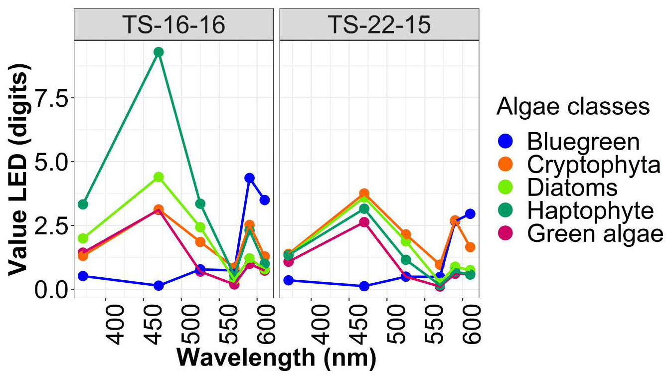
Figure 3 Different fingerprints of algae classes for each Fluoroprobe: TS-16-16 and TS-22-15.

Spectral groups were distinguished according to the relative fluorescence of chlorophyll a at 680 nm after excitation of chlorophyll a and accessory photosynthetic pigments. This differentiation utilised a manufacturer's algorithm derived from monoculture fingerprints of the main pigmentary groups (Beutler et al., 2002). The instrument can also deliver total chlorophyll a estimates (sum of all detected concentrations of algae classes). To assess the consistency among the different approaches used to estimate total chlorophyll a, we performed an intercomparison between FLP in vivo fluorescence, Turner fluorometer measurements, and extracted chlorophyll a determined by spectrophotometry. Linear regressions and correlation coefficients were used to quantify agreement between methods and to account for differences in calibration and measurement principles. The results of this intercomparison are shown in Fig. B1 in Appendix B.

This instrument can only address five spectral groups at a time, this limitation being imposed by the limited number of excitation wavelengths available. The fluorescence signal is decomposed from five independent spectral channels, which allows for the resolution of only four distinct components at most. However, new fingerprints can be recalculated with the bbe++ or FluoroProbe software in Expert mode. Algae classes defined by the manufacturer were “blue-green” (phycocyanin-rich: cyanobacteria), “green algae” (rich in chlorophyll a and b as chlorophytes and also part of the haptophyte signal; Houliez et al., 2012), “brown algae” corresponding to diatoms (xanthophyll, most dinoflagellates and part of the haptophyte signal), and “red-mix algae” (phycoerythrin-rich: mainly cryptophytes, cyanobacteria). Groups were estimated by applying an algorithm (Beutler et al., 2002) correcting the residual fluorescence of dissolved organic matter (“yellow substances”) and the turbidity (% of light transmission). Initially, the FluoroProbe TS-16-16 was supplied with fingerprints for “brown algae”, “blue-green”, “green algae” and “red-mix algae” (original fingerprints). In order to better discriminate the haptophyte Phaeocystis, a new fingerprint was recorded by Houliez et al. (2012) using natural coastal water dominated by this species. Since 2021, the manufacturer introduced a generic haptophyte fingerprint, which was incorporated into the Isochrysis fingerprint and added on the TS-22-15 FluoroProbe in 2021. Moreover, the manufacturer's name for “brown algae” is Diatoms and for “mix-red” is Cryptophyta. Thus, even though we do not agree on this nomenclature, for FAIR principles we have kept in the Database and this presentation.

Two different FluoroProbe devices were used during the 11 years of measurement, with simultaneous period: TS-22-15 (2012–2016 and 2021–2022) and TS-16-16 (2012–2022). The devices were set to measure during 2–3 min, with one acquisition every 3 s. These measurements were then averaged for each sample. Over 11 years, a total of 1253 samples were analysed by the TS-22-15 and 1835 by the TS-16-16. Outliers were determined on the basis of the correlation between total in vivo chlorophyll a fluorescence measured on the 10-AU Field Fluorometer, and the FLP total chlorophyll a estimated by the FluoroProbe. A total of 43 values were considered a posteriori as outliers (Fig. 4). These values were not included in the following study. There was a strong correlation between total in vivo chlorophyll a fluorescence on the 10-AU TD fluorometer measurements and FLP total chlorophyll a estimations: R=0.85 for TS-16-16, R=0.89 for TS-22-15 (p-value < 0.001) (Fig. 4) and after removing outliers R=0.93 (p-value < 0.001) for TS-22-15.

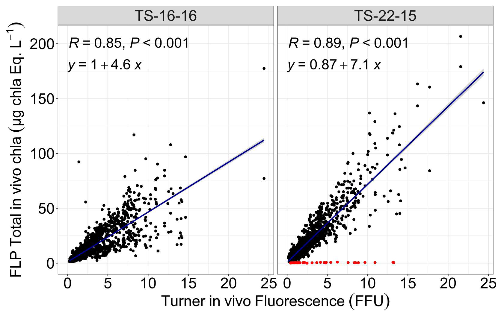
Figure 4 Outliers detection for Fluoroprobe TS-16-16 and TS-22-15. R value represent the coefficient of correlation estimated using linear regression model (blue line). y represent the equation of each blue line. The associated p-values are also provided (P). The red dots correspond to values identified as outliers.

3.4.3 Abundance and biomass of phytoplankton optical (functional) groups addressed by Automated Flow Cytometry

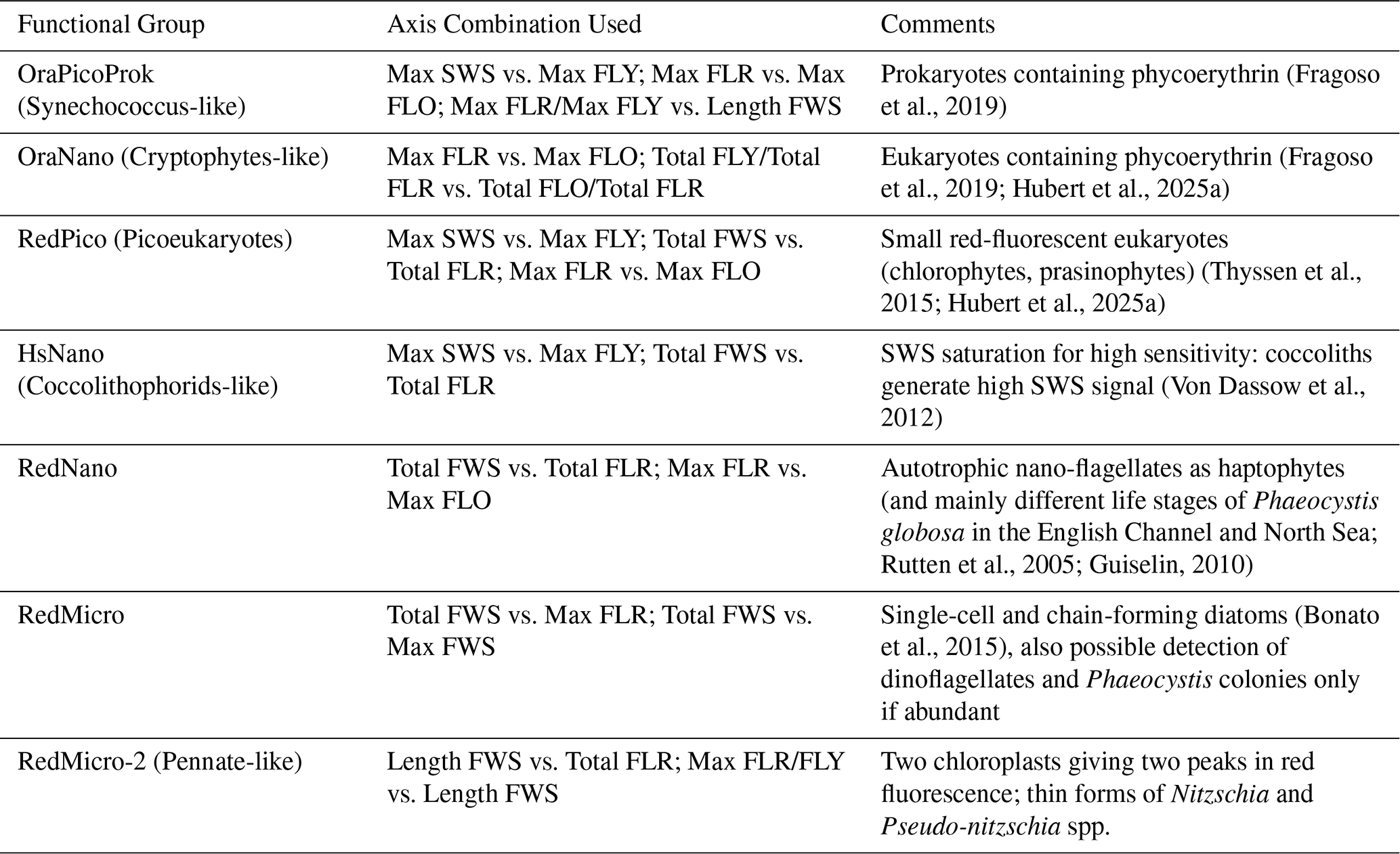
All samples were analysed in vivo after maximum 4 h of dark conservation in a cooler, followed by storage at 4 °C in a refrigerator. Analysis was performed using an automated pulse shape-recording flow cytometer (CytoSense/CytoSub). This instrument provides optical measurements at the particle level. It covers the entire phytoplankton size range from 0.1 to 800 µm width and allows to obtain abundance, size, structure and pigmentation data at the particle scale due to the use of 5 optical signals. Size and structure of pigmented cells and colonies are characterised by scattering at large and small angles (Forward Scatter – FWS and Sideward Scatter – SWS). The other three signals provide information on the pigment content of the cells and their potential physiological state through the emission of red fluorescence (chlorophyll a, FLR, 668–734 nm), orange fluorescence (phycobiliproteins: Phycoerythrin and Phycocyanin, FLO, 604–668 nm) and yellow fluorescence (Phycoerythrin, FLY, 536–601 nm) (Fontana et al., 2014; Haraguchi et al., 2017; Fragoso et al., 2019). Two protocols were used for each sample: one for small cells, called “Pico protocol” (low detection threshold, low pump speed – 5 µL s⁻¹, short duration – 5 min) and one for larger cells or “Micro protocol” (higher detection threshold, faster – between 10 and 13 µL s⁻¹, longer duration – 8 min). Using the dedicated manual classification software (CytoClus4, Cytobuoy b.v., Netherlands), 6 main functional groups were characterised, according to the interoperable vocabulary from Thyssen et al. (2022), already described in the area: OraPicoProk or Synechococcus-like cells, RedPico or picoeukaryotes, RedNano or nanoeukaryotes, HsNano or Coccolithophore-like cells, OraNano or Cryptophyte-like cells and RedMicro (diatoms and dinoflagellates bigger than 20 µm, haptophyte colonies, pigmented ciliates, filamentuous cyanobacteria (not present in our site so far; Fig. 5). For clarity, we provide a summary table (Table 1) listing each group, the corresponding cytometric axis combinations used for their identification, and their likely taxonomic affiliation based on the literature. The files were analysed by a single person to minimise interpretation bias. Fluorescent polyester beads of 1 and 3 µm (Fluospheres Carboxylate-Modified, Invitrogen, 1.0 µm, yellow-green fluorescent and Sphero brand beads, Spherotech Inc., 3.0–3.4 µm, bright intensity) were also analysed regularly to monitor measurement quality and help discriminate size classes.

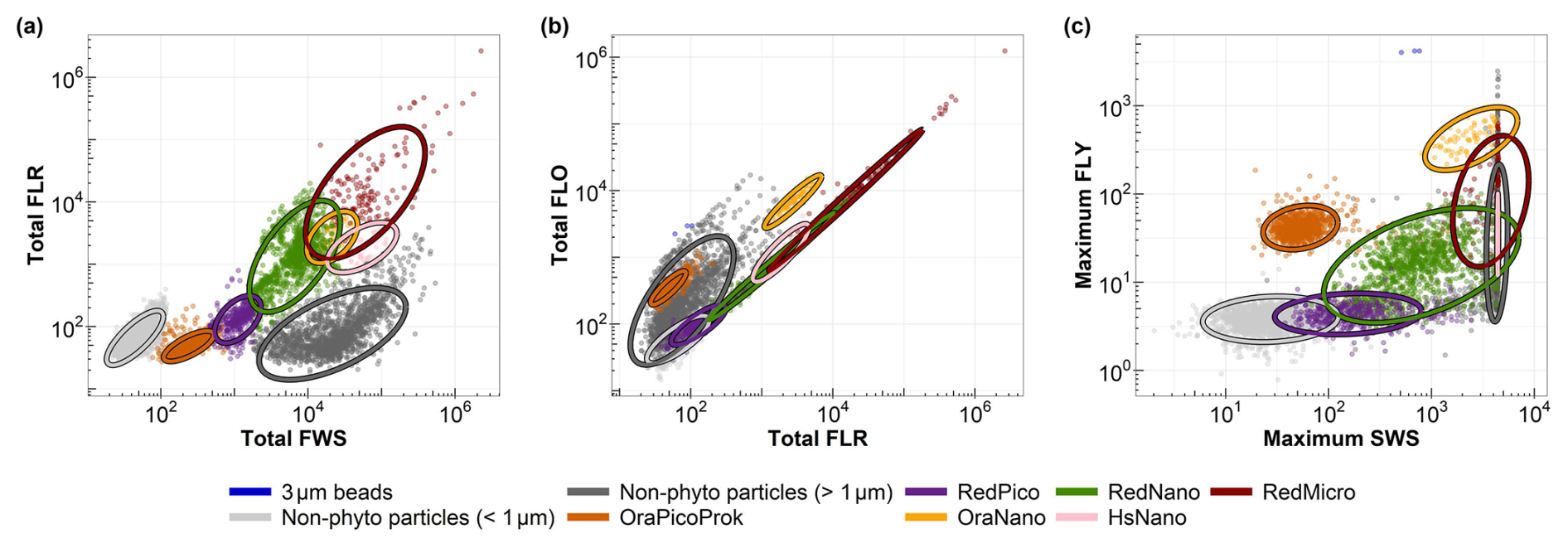
Figure 5 Cytograms showing the main groups defined during the 11 years along the DYPHYRAD transect (e.g., R0 station on 24 March 2024), characterising the main phytoplankton groups: (a) total red fluorescence (Total FLR) vs. total forward scatter (Total FWS) for the discrimination of red fluorescence groups and size class, (b) total red fluorescence (Total FLR) vs. total orange fluorescence (Total FLO) for the discrimination of orange fluorescence groups, (c) maximum yellow fluorescence (Maximum FLY) vs. maximum sideward scatter (Maximum SWS) for the discrimination of Coccolithophoridaea (HsNano). Ellipses on the graphs are calculated from a t-distribution at 95 % confidence level, aiding in accurate delineation of the respective phytoplankton groups.

(Fragoso et al., 2019)(Fragoso et al., 2019; Hubert et al., 2025a)(Thyssen et al., 2015; Hubert et al., 2025a)(Von Dassow et al., 2012)Rutten et al., 2005; Guiselin, 2010(Bonato et al., 2015)

Table 1 Combinations used to highlight different Phytoplankton Functional Groups (PFGs).

It should be noted that different Cytosense and CytoSub devices were deployed throughout the years from different funding opportunities and projects, in part to stay up-to-date with evolving technologies and also to diversify their in situ deployments. Sometimes, instruments were shipped on campaigns, implemented in fixed autonomous measuring stations or sent to maintenance, which explains the use of different machines depending on the period. During this 11-year time series, the following four instruments were used: CS-2007-15; CS-2016-78; CS-2019-93 and CS-2019-94 (Fig. 6). To ensure data comparability between instruments, intercalibration exercises were systematically performed at each machine changeover. Specifically, a set of common samples, consisting of both natural assemblages collected during routine sampling and calibration bead standards, were analysed on the outgoing and incoming instruments after acquisition settings parametrisation according Gallot et al. (2025). This procedure allowed us to verify the stability of key optical parameters (e.g., forward scatter, sideward scatter, red fluorescence, particle size proxies). When necessary, minor adjustments to the PMT voltage settings and trigger levels were applied.

Figure 6 Diagram of the use of different flow cytometers during the DYPHYRAD time-series. The dots indicate the cytometer used for each discrete sampling over time.

3.5 Database structure

The dataset is provided as a single tabular file in which each row corresponds to an individual sampling event. Columns are organised into thematic groups gathering physical, chemical, cytometric and fluorometric variables. The first columns describe the sampling context, including date, time, station identifier, and geographical position (latitude, longitude), followed by environmental measurements such as maximum sampling depth, PAR irradiance, CTD temperature and salinity, in vivo fluorescence, and the serial number of the CTD probe.

A second block of columns contains additional data from onboard sensors, including probe temperature, TSG temperature and salinity, and nutrient concentrations (nitrite, nitrate, phosphate and silicate). Cytometric variables follow, with total cell abundance and the abundance of each optical group (e.g., OraPicoProk, RedPico, OraNano, RedNano, HsNano, RedMicro), along with the serial number of the cytometer used for acquisition.

The table also includes a large set of phytoplankton spectral groups obtained from a FluoroProbe instrument. These measurements provide concentration estimates of major phytoplankton groups (e.g., blue-green algae, cryptophytes, diatoms, green algae, Phaeocystis, Isochrysis, yellow substances), as well as total chlorophyll a. Multiple configurations and wavelength combinations are included depending of serial number of FluoroProbe used (e.g., TS-16-16, TS-22-15), alongside excitation/emission values derived from different LED channels (370, 470, 525, 570, 590 and 610 nm), reported for each configuration (C: Manufacturer, P: Phaeocystis and I: Isochrysis).

All variables are accompanied by their associated units directly in the header line. Missing values are indicated as “NA”. This structure provides a comprehensive and self-contained description of the environmental context, biological measurements, and instrument metadata associated with each sampling event.

3.6 Quality control

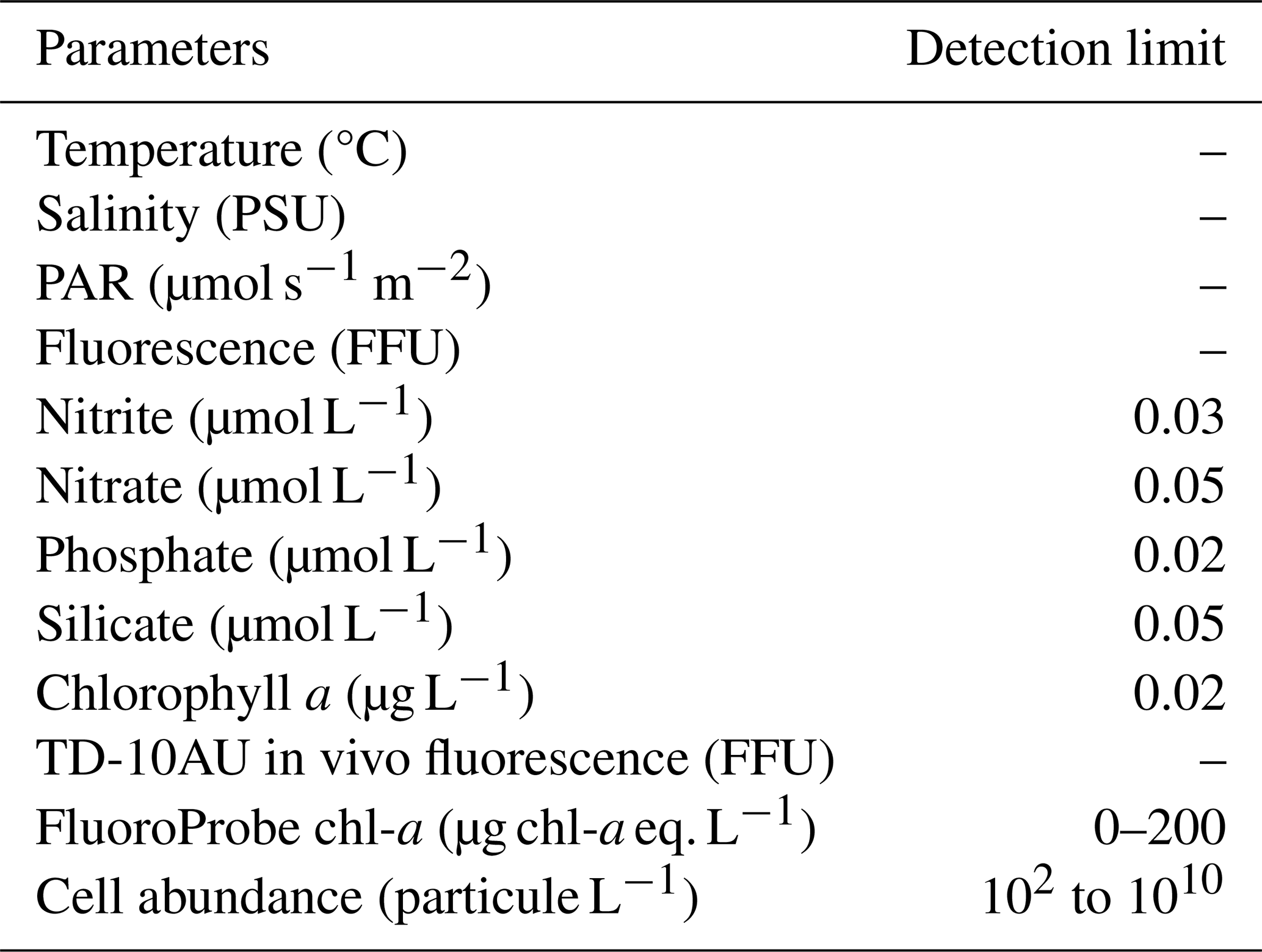
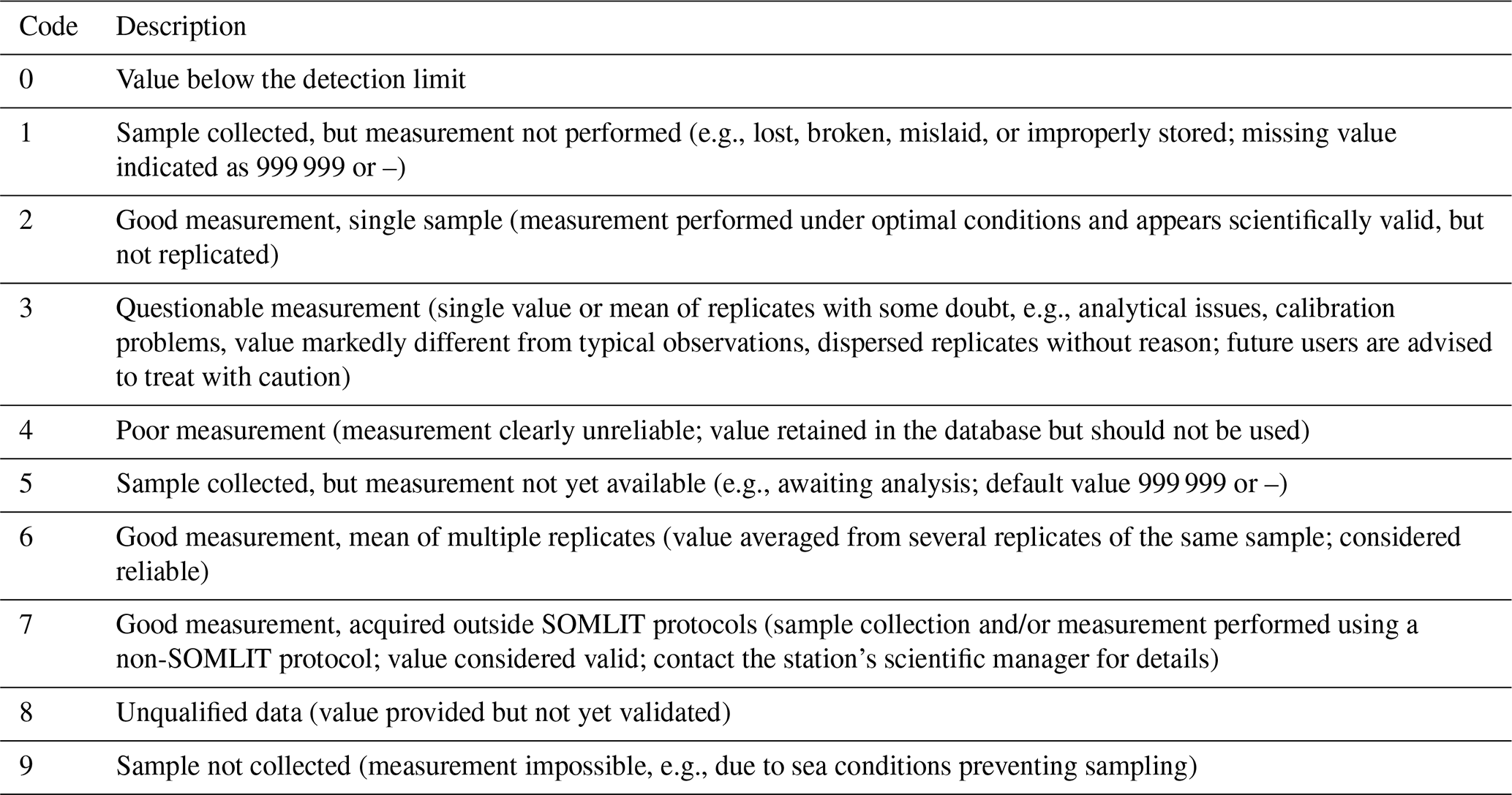
Only data with a good quality code (codes 2 and 6) are presented in this study and are available in the data set, according to Argo quality control (https://www.somlit.fr/codes-qualite/, last access: 28 January 2026; Wong et al., 2019) and translate in Table C1 in Appendix C. Based on the characteristics of each device, the detection limits of each variable are described in Table 2.

In addition to these quality flags, several post-processing steps were implemented to ensure the internal consistency of the 11-year time series. All data processing, formatting, and visualisation were carried out with R software (for further details see section Data analysis).

For cytometry files, metadata generated by the acquisition software (CytoUSB) were extracted and inspected in CytoClus4. Only files meeting predefined acquisition criteria, namely minimum sample volume and minimum number of measured particles, were retained for subsequent analyses. In addition, sensor temperature, pressure values, and other relevant acquisition metadata were systematically examined to identify potential anomalies or instrumental instabilities. Files showing atypical metadata patterns or operational issues were discarded during this quality-control step. During clustering, standard filtering was applied to remove aborted triggers, saturated signals, electronic noise, and values outside the operational range of each sensor. A consistent gating strategy was maintained across instruments and years to ensure comparability in the definition of optical groups.

Table 2 Summary of detection limit value for each parameters. The notation “–” means that there was not any detection limit.

3.7 Data analysis

Statistical analyses and data processing were performed using R software (version 4.5.0, R Core Team), using standard packages for data manipulation and visualisation (e.g. ggplot2, tidyverse, dplyr). Maps representing the study area were generated using QGIS (version 3.40.6). Cytograms were edited and finalised using CytoClus4, plotted here using R software.

4 Results and discussion

4.1 Hydrological and biogeochemical variables

The DYPHYRAD transect is characterised by a marked seasonal cycle and a spatial gradient from the coast to the offshore (Fig. E1 in Appendix E). Sea Surface Temperatures (SST) were relatively homogeneous along the longitudinal gradient of the transect, but were strongly influenced by seasonal cycle (Fig. E1A) (Lefebvre and Ambiaud, 2017). Photosynthetically Active Radiation, contrarily, showed small-scale disparities, partly linked to potential coastal turbidity and to the sampling method strategy (from offshore to the coast; Fig. E1C). Winters during the period from 2012 to 2022, were characterised by low temperatures ranging from 5.03 °C in 2013 to 13.06 °C in 2022 (mean: 8.43 ± 1.84 °C, Fig. 7) and relatively low levels of PAR, ranging from 3 µmol s⁻¹ m⁻² in 2021 to 528 µmol s⁻¹ m⁻² in 2017 (mean: 130 ± 106 µmol s⁻¹ m⁻², Fig. 7). Spring is a transition period during which SST began to rise, with values ranging from 5.21 °C in 2013 to 15.99 °C in 2017 (mean 9.79 ± 2.32 °C), and a PAR ranging from 12 in 2014 to 1209 µmol s⁻¹ m⁻² in 2015 (mean: 348 ± 243 µmol s⁻¹ m⁻²).

Figure 7 Boxplots of sea surface CTD parameters by season and year along the DYPHYRAD transect from 2011 to 2022. The variables represented are temperature, salinity and PAR. The dots indicate outliers. All surface stations sampled from 2012 to 2022 were grouped by season.

Surface waters warmed considerably during the summer, with temperatures ranging from 11.70 °C in 2013 to 20.57 °C in 2022 (mean: 16.26 ± 1.57 °C). This warming was controlled by PAR, which was relatively high in summer, ranging from 19 in 2015 to 1360 µmol s⁻¹ m⁻² in 2022 (mean: 487 ± 343 µmol s⁻¹ m⁻²). Autumn is characterised by a decrease in average PAR (mean: 234 ± 266 µmol s⁻¹ m⁻²) despite maximum values that may still be close to those of summer (maximum: 1722.56 µmol s⁻¹ m⁻² in 2019). A similar pattern is also observed for surface water temperatures (between 9.90 °C in 2016 and 20.66 °C in 2022; mean of 16.30 ± 2.55 °C).

Over these 11 years, SST appear to have increased, particularly in winter. This increase in SST was in line with previous observations in the area and on a global scale (Saulquin and Gohin, 2010; Auber et al., 2017; Ruela et al., 2020). The warmest year of our time series for all seasons was 2022. In terms of PAR, the greatest variation was observed in summer 2022, with mean PAR considerably higher than in the other years. This follows the heat wave observed during the summer of 2022, with average sea surface temperatures throughout France between +1.3 and +2.6 °C above the long-term average (1982–2011), linked to high air temperatures and above-average surface PAR and below-average total cloud cover (Guinaldo et al., 2023).

As for salinity, the area was not characterised by a seasonal cycle (Lefebvre and Ambiaud, 2017), with relatively slight variations between spring (mean: 34.13 ± 0.43 PSU), summer (mean: 34.35 ± 0.33 PSU) and autumn (mean: 34.29 ± 0.40 PSU). However, within these seasons, there are major disparities from one year to the next, with more widespread extreme values (min: 32.23 in spring 2021 to 34.69 PSU in summer 2017; max: 33.97 in spring 2020 to 35.11 PSU in spring 2017). Salinity values were highest at the offshore stations and have been marked by strong desalination in 2020. The month of February 2020 was marked by major storms (“Ciara”, “Inès” and “Dennis”) which influenced the wind and therefore the mixing of the water column as well as freshwater inflows (Galvin, 2022). EEC is characterised by the influence of strong freshwater flows, linked to the many estuaries along the French coast, and by periods of heavy precipitation (Taylor et al., 1981). Only winter season stood out, with lower values ranging from 29.65 to 34.97 PSU (mean: 33.9 ± 0.58 PSU, Fig. 7). Winter salinity variations seem to occur over several years, with cycles of high values (for the years 2012, 2015 to 2017 then 2021 and 2022) and low values (2013, 2014, 2018, 2019 and 2020).

Spatially, all nutrients exhibited pronounced spatial and temporal heterogeneity (Fig. E2). However, nitrates displayed a strong coastal-offshore gradient. This gradient can be attributed to the influence of rivers and rainfall on the concentration of dissolved inorganic nitrogen along the French coast (Dulière et al., 2019). The Strait of Dover is subject to pronounced seasonal nutrient cycles, and this phenomenon is especially marked in the coastal zone due to inputs, particularly from the French coast (Bentley et al., 1993). These inputs follow the “river flow” ROFI and include brackish waters from the Somme to the Slack estuary (Brylinski et al., 1991), characterised by high concentration of phosphate, silicate, nitrate and nitrite concentrations during winter (Fig. 8).

Nitrate concentrations were very high in fall and winter at the beginning of the series (2012 to 2014), after this period, these values decreased by half. Summer nitrate concentrations were the lowest of the four seasons (0.57 ± 0.64 µmol L⁻¹) and a relatively modest maximum (4.34 µmol L⁻¹). However, nitrates were extremely variable in spring, despite the same average as in fall (mean: 2.41 ± 4.26 µmol L⁻¹), with the highest maximum of the four seasons (55.85 µmol L⁻¹). In fact, Gentilhomme and Lizon (1997) already showed that nitrate stocks are reestablished during the winter period and then decrease during spring bloom until depletion, which is consistent with the dynamics observed in this study and the variability observed during the spring. Spring is characterised by strong variability in nutrient concentrations due to transitional phases before and after phytoplankton blooms. Before the bloom season, nutrient levels are generally higher, whereas after the bloom, depletion occurs due to increased phytoplankton uptake, leading to fluctuating concentrations throughout the season. During this period, phosphorus (P), silicate (Si), and nitrogen (N) are sequentially depleted from late winter to late spring. P is the first to reach limiting concentrations, followed by Si and then N. This depletion pattern supports the persistence of Phaeocystis blooms, as these organisms can utilise dissolved organic phosphorus (DOP) and do not require Si for growth (van Boekel et al., 1992; Lancelot et al., 2005; Passow et al., 2007; Chai et al., 2023).

The years with the highest mean concentrations were 2018, 2019, 2021 and 2022 for silicates, and 2012 for phosphates, influenced by high winter concentrations (Fig. E2C and D). Phosphate and silicate concentrations were also relatively high in fall with respective maximum concentration of 0.837 µmol L⁻¹ (mean: 0.22 ± 0.14 µmol L⁻¹) and 9.59 µmol L⁻¹ (mean: 2.35 ± 2.33 µmol L⁻¹). Previous studies showed an increase in nutrient concentration in the waters of EEC and southern North Sea since 1930 (Laane et al., 1993). These nutrient stocks play an important role in the spatio-temporal dynamics of phytoplankton (e.g., diatoms or Pheaocystis) (Karasiewicz et al., 2018). Over the past eleven years, phosphate concentrations have tended to rise in fall and winter, and decrease in summer. We hypothesise that increased release of dissolved inorganic phosphorus (DIP) from particulate inorganic phosphorus (PIP) occurs due to adsorption-desorption processes, particularly intensified by storms or heavy rainfall that leach soils during winter and fall. On the other hand, the highest phosphate values were found in winter 2020.

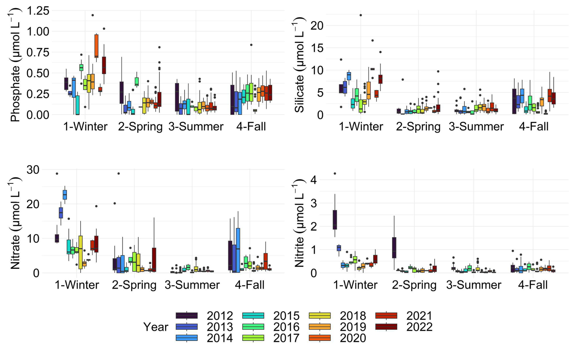
Figure 8 Boxplots of nutrient concentration for each season of each year. The dots indicate outliers. All surface stations sampled from 2012 to 2022 were grouped by season.

Coastal waters showed the greatest variability in environmental parameters due to their shallower depth, greater surface area for exchange with the atmosphere and the seabed (including suspended particles), and significant freshwater inputs from rivers and runoff. These factors contribute to fluctuating temperature, salinity and nutrient levels, making nearshore coastal ecosystems more dynamic than offshore coastal environments.

4.2 Phytoplankton measurements: pigment analysis and automated measurement

4.2.1 Total chlorophyll a estimated by in vivo mono-spectral fluorometry, pigment extraction and FLP Total chlorophyll a

The DYPHYRAD transect was subject to seasonal variations in measured and estimated concentration of chlorophyll a. Stations nearest the coast had the highest values and showed the most marked seasonal variations (Fig. E3). Only years 2013 and 2021 showed a spring bloom that spreads across the entire coastal-offshore transect. This phenomenon was spatially well represented by the three methods. Conversely, some years blooms were concentrated at the coastal station, e.g. from 2016 to 2019, this trend was more marked for the FLP estimation of the total chlorophyll a equivalents (Fig. E3C).

Regardless of the method used to estimate total phytoplankton biomass (chlorophyll extraction, in vivo fluorescence, or FluoroProbe), the highest values are consistently observed in spring (Figs. 9 and 10), as reported by previous studies (Breton et al., 2000; Schapira et al., 2008; Lefebvre et al., 2011; Belin et al., 2012; Hernandez Farinas et al., 2020). This period is generally favorable for bloom development, as light intensity and photoperiod increase, associated to better weather conditions. In addition, nutrient stocks are relatively high in winter, as phytoplankton growth is limited by reduced light availability and low temperatures. However, occasional blooms can occur in winter at these latitudes if conditions are favorable. This allows nutrients to accumulate in the water column. The regeneration of nutrient stocks is also due to increased inputs from estuaries, rain and runoff, which transport nutrients of terrestrial origin into the marine system. Spring chlorophyll a concentration ranged from 0.2 to 23.1 µg L⁻¹ (mean: 4.88 ± 3.4 µg L⁻¹) (Fig. 9), while in vivo chlorophyll a fluorescence ranged between 0.29 and 14.650 FFU (mean: 3.14 ± 2.66 FFU; Fig. 10) whereas FLP Total in vivo chlorophyll a equivalents ranged between 2.69 and 107.91 µg chl-a eq. L⁻¹ (mean: 20.23 ± 17.05 µg chl-a eq. L⁻¹) (Fig. 11). During this period, the highest phaeopigment concentrations were recorded, with values ranging from 0 to 18.50 µg L⁻¹ (mean: 1.49 ± 1.28 µg L⁻¹). Chlorophyll a and pheopigments concentrations decreased during summer, at different times and magnitude depending on the year. Particularly, intense spring blooms were observed in 2013 and 2021, as indicated by chlorophyll a concentrations. This trend was well reflected with in vivo fluorescence for 2021, but slightly underestimated for 2013 (one of the major spring blooms of the series appeared to be for the year 2014 instead). Other blooms were less intense, either starting in late winter to early spring or beginning later but persisting over a longer period. For instance, in 2016, chlorophyll a and in vivo fluorescence levels remained relatively stable during both spring (mean: 3.04 ± 1.66 µg L⁻¹ and 3.52 ± FFU) and summer (mean: 3.49 ± 3.24 µg L⁻¹ and 1.90 ± 0.82 FFU). By contrast, 2013 or 2017 saw an early bloom, with winter maxima of 11.77 and 6.05 µg L⁻¹ for chlorophyll a, respectively (mean: 3.87 ± 4.76 and 2.52 ± 1.74 µg L⁻¹). The timing and intensity of spring blooms (whether early and low or late and high) can be influenced by various factors, including limited light availability caused by turbidity from suspended sediments or competition with diatoms (Guiselin, 2010). Lastly, 2020 was unusual in that very few data were acquired during the spring period because of the pandemic lockdown, so these spring values could not be considered representative of a bloom or only late spring–early summer one. In autumn, average chlorophyll a and in vivo fluorescence values were low and fairly constant, as reported in previous studies (Lefebvre and Ambiaud, 2017). It would appear that values vary more during the winter period, particularly for pigment extraction method. However, this variability could partly be attributed to a lower sampling rate, as worsening weather heavily impacts sample collection, which is highly dependent on weather conditions.

Figure 9 Boxplots of chlorophyll a concentration (µg L⁻¹) and Phaeopimgent concentration (µg L⁻¹) for each season of each year along the DYPHYRAD transect. The dots indicate outliers. All surface stations sampled from 2012 to 2022 were grouped by season.

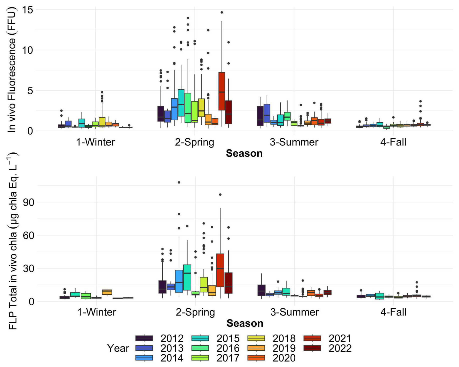
Figure 10 Boxplots of in vivo chlorophyll a fluorescence (FFU) and FluoroProbe Total chlorophyll a estimates (µg chl-a eq. L⁻¹) for each season of each year over the whole DYPHYRAD transect. The dots indicate outliers. All surface stations sampled from 2012 to 2022 were grouped by season.

4.2.2 Phytoplankton spectral (pigmentary) groups addressed by in vivo multi-spectral fluorometry

Multi-spectral fluorescence allows differentiation of up to four spectral (pigmentary) groups. The seasonal and annual data presented in this study focus on the FluoroProbe TS-16-16 device, as it provided the longest time series with the highest sampling frequency. However, similar data for TS-22-15 is also available in the dataset. The FluoroProbe was used to characterise the phytoplankton community assemblage with three common fingerprints (“brown”, “blue-green” and “mix-red”) and a choice made between two different fingerprints: Green Algae or Phaeocystis (Fig. 11). Phaeocystis was the main Haptophyte in our study area (Astoreca et al., 2009; Lefebvre et al., 2011). As a result, seasonal concentrations was represented only for this fingerprint, although the full dataset remains available. Data from TS-22-15 are not represented in this study because the haptophyte fingerprint was obtained in two different ways (local Phaeocystis fingerprint, then Isochrysis haptophyte fingerprint installed by the manufacturer) and this instrument has been used in a more heterogeneous way (no data between 2017 and 2021).

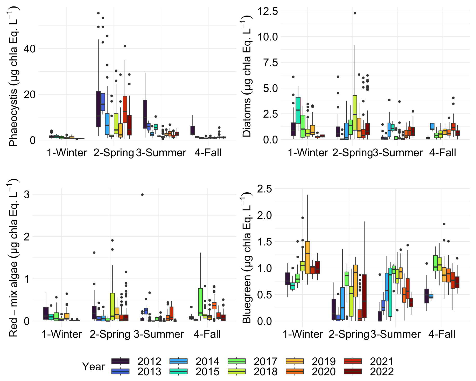
Figure 11 Boxplots of phytoplankton spectral (pigmentary) groups addressed along the DYPHYRAD transect with the Fluoroprobe (including the Phaeocystis fingerprint) for each season of each year. The dots indicate outliers. All surface stations sampled from 2012 to 2022 were grouped by season.

Fairly marked seasonal variations were observed, as stated in previous studies (Lancelot et al., 1998; Grattepanche et al., 2011) and on the same coastal-offshore transect (Houliez et al., 2013), notably for Phaeocystis and Diatoms (Fig. 11). The start of the bloom for “brown algae” (mainly diatoms here) is in late winter, with more productive years between 2012 and 2017 (3 µg chl-a eq. L⁻¹). As expected, spring was confirmed to be a productive period for the “brown algae” with particular years like 2017 and 2018 (2.50 µg chl-a eq. L⁻¹). In summer and fall, diatom concentration in chlorophyll a equivalents were generally similar, with slightly higher values observed in fall 2014 and 2021 (Fig. 11). Generally, a succession of phytoplankton typical of the EEC is characterised by a late winter or early spring. Diatom bloom followed by a Phaeocystis spring bloom (Breton et al., 2000; Guiselin, 2010; Grattepanche et al., 2011). We observed this phenomenon in our time series for years 2012, 2015, 2017 and 2019. Diatoms blooms are linked to the concentration of silicates in the environment, these stocks were high in winter, then decreased during the bloom (Fig. 8) and became a limiting factor (Rousseau et al., 2000). This phenomenon can also be linked to the seasonality of the amount of available light (Peperzak et al., 1998). For Phaeocystis, spring was the most productive period, with highest values in 2013 (17 µg chl-a eq. L⁻¹) and 2021 (15 µg chl-a eq. L⁻¹). Phaeocystis developed a maximum biomass in spring (Fig. 11) in the English Channel (Belin et al., 2012). It represented between 28 % and 90 % of the total chlorophyll a estimated in vivo over the entire time series (Fig. 12). These blooms are stimulated by nitrate and phosphate enrichment (Lancelot et al., 1998; Lefebvre and Ambiaud, 2017), from nutrient inputs from rivers, exchanges with offshore water masses and with sediment from shallow areas (Reynolds, 2006). Our PAR data indicate that light availability is low during winter and increases in spring (Fig. 7), consistent with seasonal light limitation, and our phytoplankton data show that diatom blooms consistently precede Phaeocystis blooms in spring (Fig. 14), supporting the idea that both light availability and inter-specific competition contribute to bloom timing and intensity and grazing/viral lysis (not studied) to their decay.

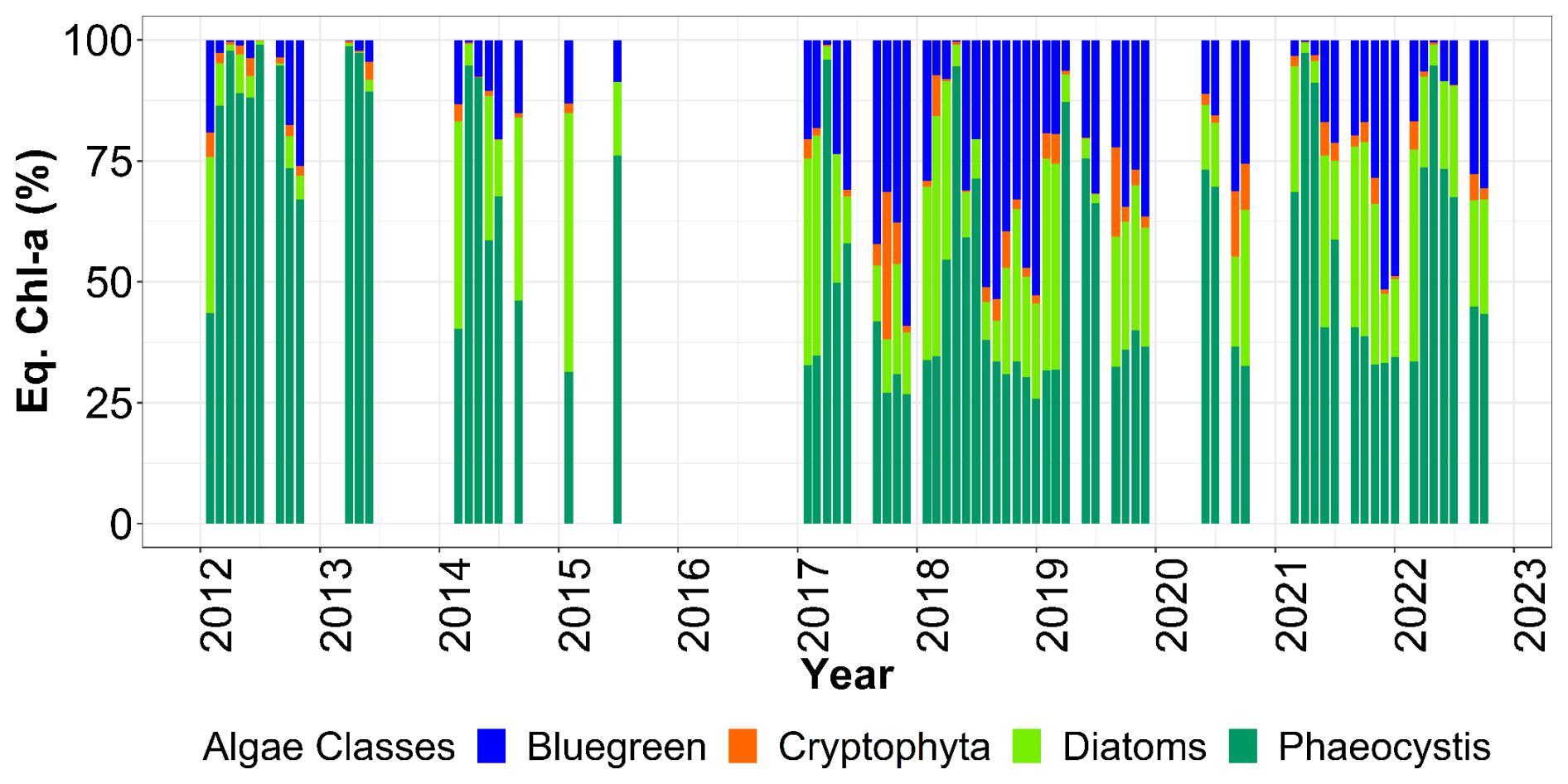
Figure 12 Relative contribution (%) of Fluoroprobe-defined spectral groups along the DYPHYRAD transect to FLP Total chlorophyll a estimation, with Phaeocystis fingerprint of TS-16-16 device.

The red-mix algae spectral group (Cryptophyes, cyanobacteria showing Phycoerythrine as major pigment) varied very little throughout the year and were the minority group in our study area, as reported in previous studies, with less than 10 % maximum over 11 years (Fig. 12; Houliez et al., 2013; Lefebvre and Poisson-Caillault, 2019). The “blue-green” group (cyanobacteria of Phycocyanine as major pigment) was highly variable in spring and summer, with concentrations ranging 0 (corresponding to undetected values) to 1 µg chl-a eq. L⁻¹. A marked trend emerged in summer, with a 5-year period of marked increase starting in 2012 with a peak in 2017, followed by a 5-year period of decline until 2022 (Fig. 11). An increase was evidenced in fall from 2017 onward compared with previous years (25 % of total concentration; Fig. 12), then from 2019 the trend was downwards for this season. Conversely, in winter over 11 years, this group show an apparent increasing trend between 2015 and 2019, followed by a period of sharp decline in 2021 and 2022.

4.2.3 Abundance and biomass of phytoplankton optical (functional) groups addressed by Automated Flow Cytometry

The variability in phytoplankton groups, analysed through automated flow cytometry, defined pronounced spatial patterns, with OraPicoProk (i.e. Synechococcus sp.) showing higher abundances in offshore than in coastal waters (Fig. E4A). The years 2015 to 2018 showed this spatial pattern in particular. The year 2021, on the other hand, showed the highest abundances observed for this group, provoking a less pronounced coastal-offshore gradient. For the RedPico (i.e. picoeukaryotes) and OraNano (i.e. cryptophytes) groups (Fig. E4B and C), there was no coastal-offshore gradient, but an increase in abundance within these groups from year 2019 onwards. The RedNano and RedMicro groups showed higher abundances close to the coast, with a particularly marked bloom in 2015 for RedNano (mainly represented by Phaeocystis globosa Scherffel free flagellates and colonial cells during the spring bloom and other nanoeukaryotes during the rest of the time) and 2013 for RedMicro (i.e. diatoms, pigmented dinoflagellates and, if highly concentrated, Phaeocystis colonies). Total abundance showed no regular pattern and seemed to depend on the very high abundance of different groups such as OraPicoProk (Fig. E4F).

Over time, this series allowed to follow the succession of phytoplankton communities, with a clear dominance of OraPicoProk and RedPico, except during the spring when RedNano dominated the community by almost 90 % (Fig. 13). This very large abundance of RedNano in spring is consistent with the well-known P. globosa Scherffel bloom in the area (Breton et al., 2000; Grattepanche et al., 2011; Lefebvre et al., 2011; Breton et al., 2022). Flow cytometry can discriminate its different life stages, allowing haploid, diploid, and colonial cells to be distinguished (Rutten et al., 2005; Guiselin, 2010; Houliez et al., 2012; Bonato et al., 2015) but not shown here. The strongest RedNano spring bloom recorded in the time series was in 2015 with maximum abundance of $\mathrm{3.20}\times {\mathrm{10}}^{-\mathrm{4}}$ cell mL⁻¹ (R0 station on 22 May). The summer of 2021 was the most abundant in total phytoplankton cells, largely dominated by the highest abundance of OraPicoProk with an abundance of $\mathrm{5.44}\times {\mathrm{10}}^{-\mathrm{4}}$ cell mL⁻¹ (R1 station on 23 June). The dominance of OraPicoProk in summer, and particularly in the hottest summers (as in the summer 2022), can be explained by an optimum temperature in the growth rate of Synnechococcus spp. at high temperatures (Pittera et al., 2014; Robache et al., 2025). The abundance of RedPico exhibited a clear seasonal variation, with a higher abundance observed during summer and fall (Fig. 14). The peak of RedPico abundance was recorded in summer 2020. A multi-year increase in RedPico and OraPicoProk has already been observed over the last decade (Hubert et al., 2025c). In the English Channel, RedPico is predominantly composed of Chlorophyta (Marie et al., 2010; Masquelier et al., 2011). The OraNano, HsNano and RedMicro groups made a minimal contribution to total phytoplankton abundance. RedMicro cells (as well as RedNano), though less abundant than smaller cells and responsible for phytoplankton blooms before and after Phaeocystis globosa Scherffel blooms, nevertheless make up a large part of the biovolume, chlorophyll content (FLR, not shown) and biomass in the EEC.

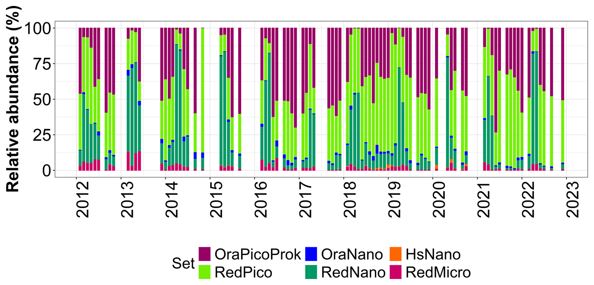
Figure 13 Relative abundance (%) of PFGs over the whole DYPHYRAD transect (average values over the 9 stations), over time (2012 to 2022).

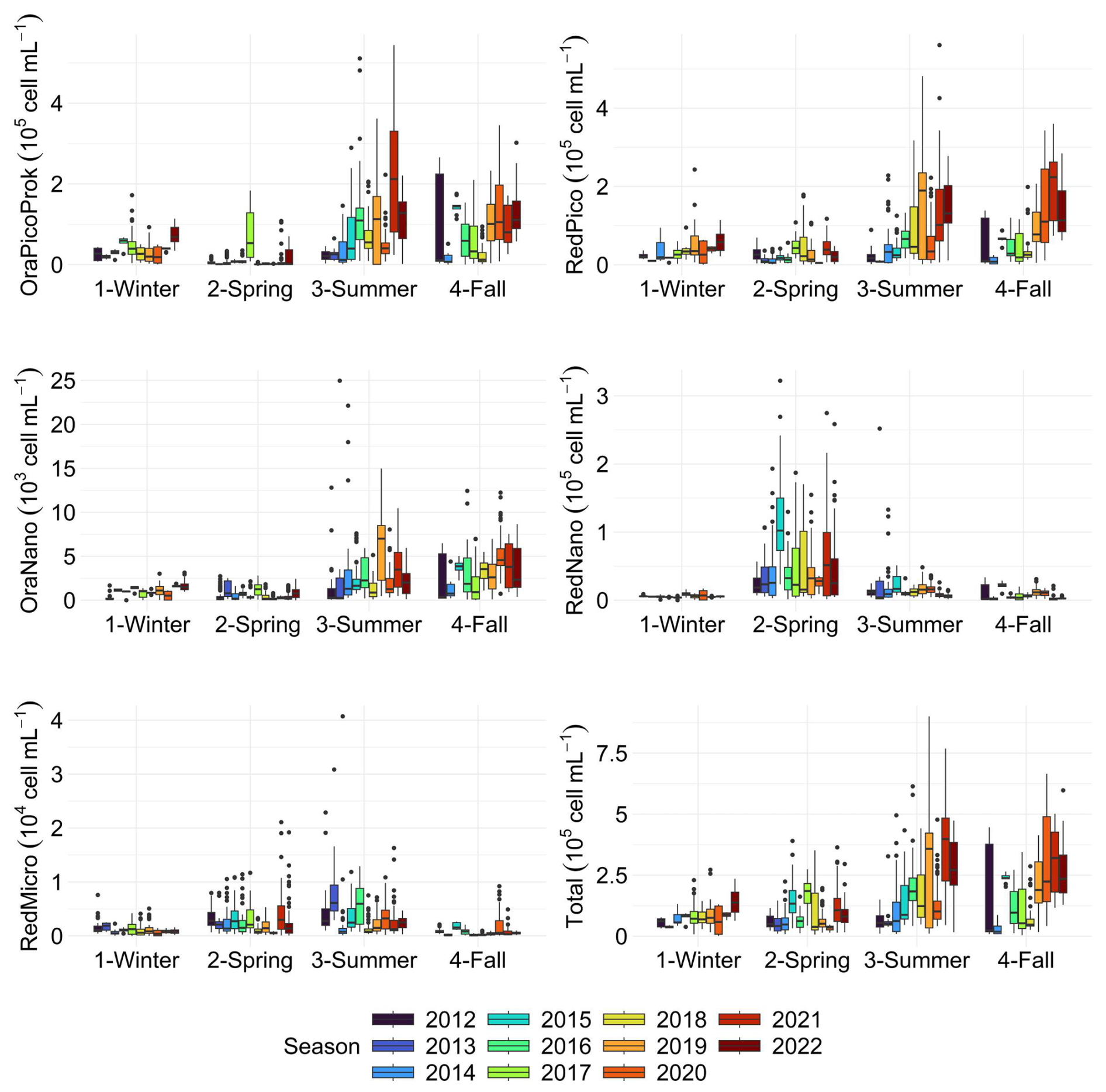
Figure 14 Boxplots of PFGs abundance for each season of each year. The dots indicate outliers.

4.3 Potential Applications

4.3.1 Case of Phaeocystis globosa Scherffel

Phaeocystis globosa Scherffel represents one of the most ecologically significant prymnesiophytes in the region, frequently contributing to spring blooms and playing a central role in biogeochemical cycling. The environmentally disturbed area, and more specifically the enrichment of nitrates combined with a depletion of silicates at the end of winter, promotes the annual spring proliferation of P. globosa Scherffel (Skouroliakou et al., 2022). Analysis of our time-series indicates that P. globosa Scherffel typically develops during the early spring period, with maximum abundances observed between March and May. Interannual variation was observed, with particularly pronounced blooms in 2022, which may reflect variability in environmental conditions such as nutrient availability and temperature. These observations are consistent with previous studies reporting recurrent spring blooms and highlight the importance of P. globosa Scheffrel as a recurring component of the phytoplankton assemblage in the area.

According to FluoroProbe data, P. globosa Scheffrel can dominate the phytoplankton community during spring, accounting for up to 80 % of total equivalent chlorophyll a in some years. This pronounced dominance strongly influences the in vivo fluorescence signal, as shown by concurrent peaks (Figs. 10 and 12) during the spring period. The high contribution of P. globosa Scheffrel to total chlorophyll explains the marked seasonal increase in fluorescence observed between late winter and spring, while its decline later in the year corresponds to reduced fluorescence levels and a shift toward diatom dominance. The same pattern was observed with RedNano abundance (Fig. 14). These results clearly indicate that P. globosa Scheffrel plays a major role in driving the seasonal and interannual variability of total in vivo chlorophyll fluorescence in this coastal system.

The detailed time-series data on Phaeocystis globosa Scherffel provide several potential applications. First, they can be used to improve predictive models of spring bloom dynamics, allowing for better forecasting of bloom timing and intensity based on environmental drivers such as nutrient availability. Second, the ability to track P. globosa Scheffrel dominance in near real-time using in vivo fluorescence and FluoroProbe data can support early warning systems for ecosystem monitoring, including potential impacts on local fisheries and aquaculture due to bloom-associated changes in water quality. Third, the quantification of P. globosa Scheffrel's contribution to total chlorophyll can inform biogeochemical models, particularly regarding carbon and sulfur cycling, as this species is known for its role in dimethylsulfide (DMS) production and particulate organic carbon export. Finally, these datasets provide a valuable baseline for assessing long-term trends in phytoplankton community composition under changing environmental conditions, helping to disentangle natural interannual variability from anthropogenic impacts.

4.3.2 Analyses of seasonnal, interannual and long term variability

Long-term analyses of seasonal and interannual variability are particularly valuable for detecting decadal or long-term changes in phytoplankton communities. As shown by Hubert et al. (2025c), automated flow cytometry provides high-resolution data that reveal shifts in community composition, highlighting trends that may be linked to environmental change or anthropogenic pressures and discuss about size community composition.

4.3.3 Satellite product validation and algorithm development

The availability of long-term, large-scale datasets from ocean-colour satellites opens promising avenues for validating our in situ observations and developing tailored chlorophyll a retrieval algorithms. For example, Roy et al. (2013) demonstrated how satellite-derived size-spectrum estimates of phytoplankton can be used to infer community structure and its temporal evolution at global scale. By combining our high-frequency field data (fluorescence, pigment extraction, cytometry) with collocated satellite reflectance data, we could assess the performance of existing ocean-colour chlorophyll a products in our coastal study area, develop or calibrate regionally tuned algorithms taking into account the local optical complexity (e.g. high CDOM, suspended matter, community composition), and produce synoptic spatial-temporal maps of phytoplankton biomass or spectral/size-class composition.

4.3.4 Coastal monitoring and environmental assessment

Long-term and systematic monitoring of coastal waters is key for environmental assessment and management. As illustrated in the OSPAR plankton community assessment (Louchart et al., 2023), changes in phytoplankton and zooplankton composition provide essential indicators of ecosystem health and anthropogenic or climatic pressures. By coupling our high-frequency in situ measurements (chlorophyll a, fluorescence, flow cytometry) with environmental parameters, our dataset contributes to ongoing coastal monitoring efforts. In particular, it can help detect shifts in community structure, assess the occurrence and frequency of bloom events (including potential harmful algal blooms), and evaluate long-term trends in water quality and ecosystem functioning. Moreover, such datasets support early warning systems and inform coastal management, conservation or aquaculture practices by providing robust baselines against which future changes can be compared.

5 Data availability

The DYPHYRAD dataset is available at https://doi.org/10.17882/104524 (Hubert et al., 2025b).

6 Conclusions

The dataset derived from the DYPHYRAD surveys deploying automated in vivo measurements at high spatial resolution with innovative optical sensors provided insights into the coastal-offshore phytoplankton variability and weekly, seasonal and inter-annual dynamics for 11 years. These data, addressing phytoplankton functional diversity, should be useful to contribute to the calculation of indicators to describe the state of the pelagic environment (Rombouts et al., 2019), to feed models that could predict algal blooms in the EEC, to study the structure and dynamics of phytoplankton community functional assemblies, and/or to model and improve our understanding of the impact of anthropogenic pressures and climate change on this marine ecosystem. By covering the full phytoplankton size range through in vivo automated measurements on a weekly basis and at a fine spatial scale, this approach complements fortnightly to monthly monitoring services and networks. It enables the integration of functional data into trophic models, thereby supporting the management of living resources. This monitoring is planned to continue, having been recognised as valuable to the French research community by the IR ILICo, which unites all national observation services. It also holds potential for expansion, including the integration of additional applications such as automated imaging.

Appendix A: Sampling coordinates and general statistics of dataset

The Table A1 shows the coordinates of the 9 transect sampling points in decimal degrees. The Table A2 represents the descriptive statistics for the parameters measured during DYPHYRAD cruises from 2012 until 2022. The table shows the number of total discrete measurements made, as well as the distribution of data via median, first and third quartile. The number of missing values is also reported, which may be due to a measurement problem related to the instrument.

Table A1 Coordinates of DYPHYRAD transect stations.

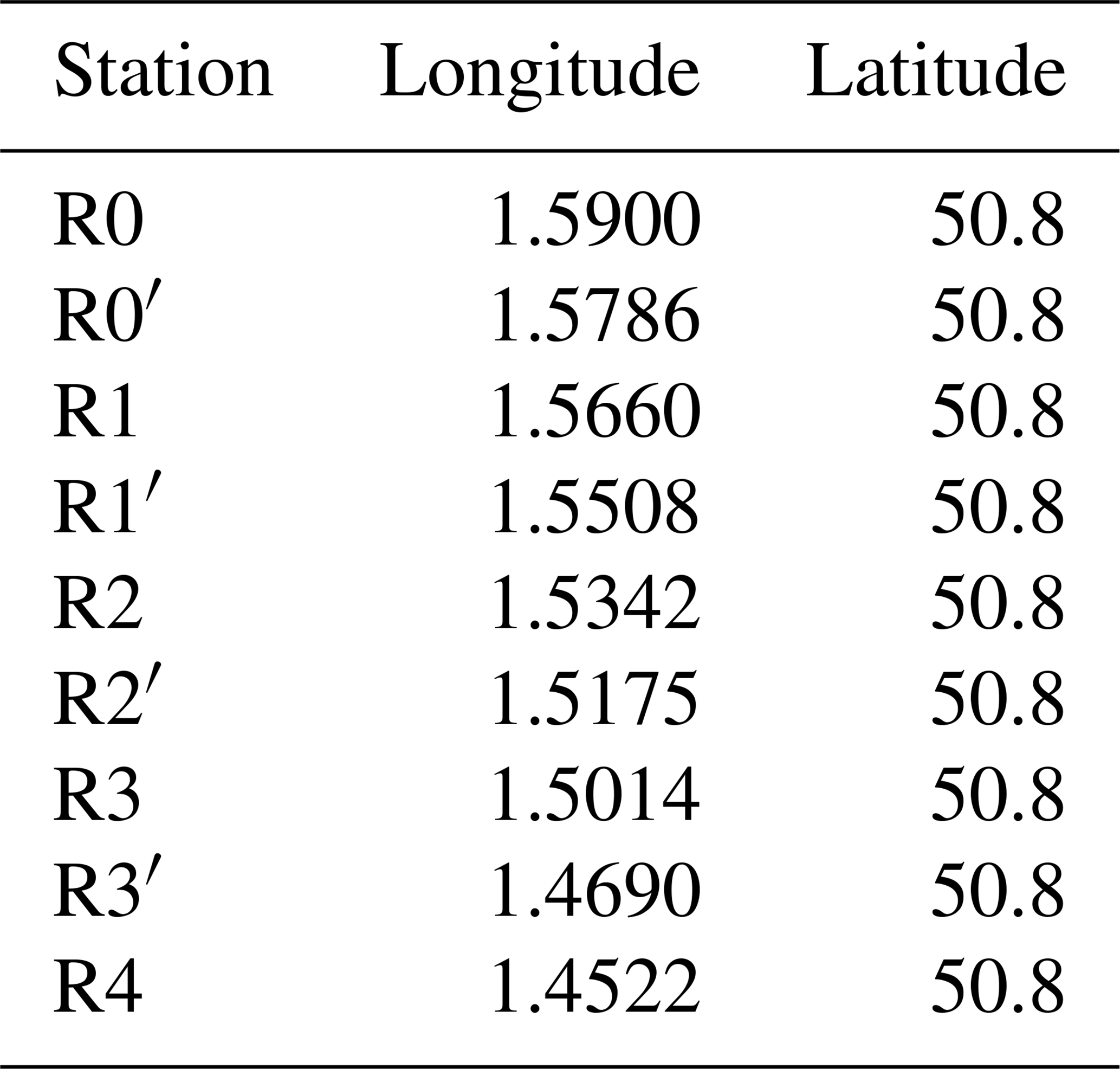
Table A2 Descriptive information of the dataset: the size (n), minimum and maximum values (Min and Max), first and third quartiles (Q1 and Q3), median, mean and number of missing data (NAs).

Appendix B: Intercomparison

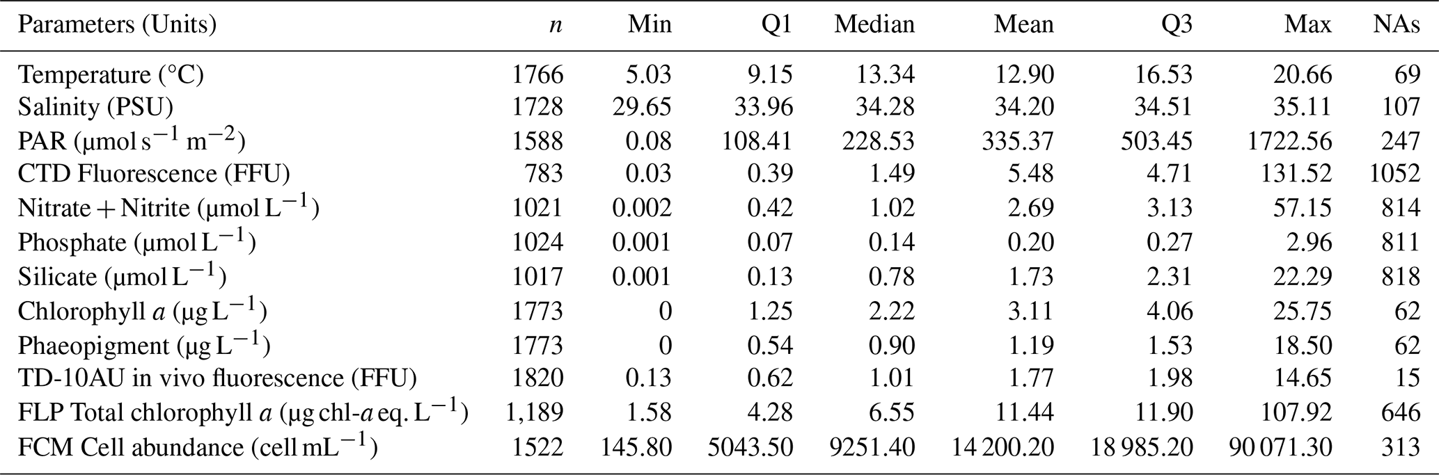
Figure B1 Inter-method comparison of three approaches for estimating chlorophyll-a concentration.

Appendix C: Quality control

Table C1 Translation of SOMLIT quality codes.

Appendix D: FluoroProbe green algae fingerprint

The FluoroProbe was also used to characterise the assembly of the phytoplankton community in complement of previous results obtain with Phaeocystis fingerprint (shown in the main results section of the paper) with common fingerprints based on that defined by the manufacturer “brown”, “blue-green” and “red-mix” and “green algae” (Figs. D1 and D2).

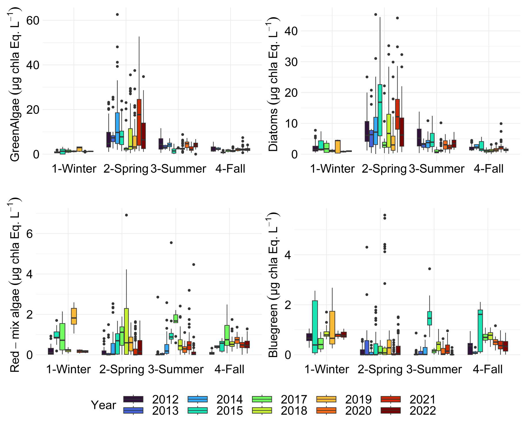
Figure D1 Boxplots of phytoplankton spectral (pigmentary) groups addressed with Fluoroprobe TS-16-16 (including the Green algae manufacturer fingerprint) for each season of each year. The dots indicate outliers. All surface stations sampled from 2012 to 2022 were grouped by season.

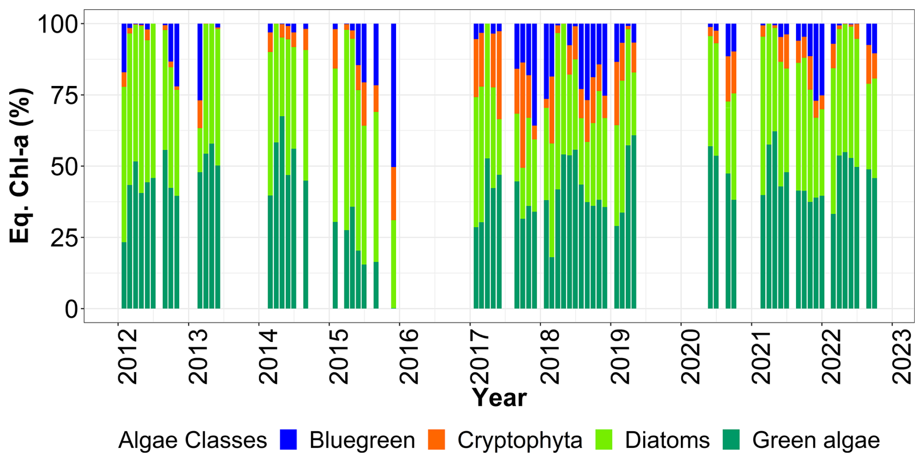
Figure D2 Relative contribution (%) of Fluoroprobe-defined spectral groups to FLP Total chlorophyll a estimation, with Green algae fingerprint of TS-16-16 device along the DYPHYRAD transect, from 2012 to 2022.

Appendix E: Spatial variability along the transect

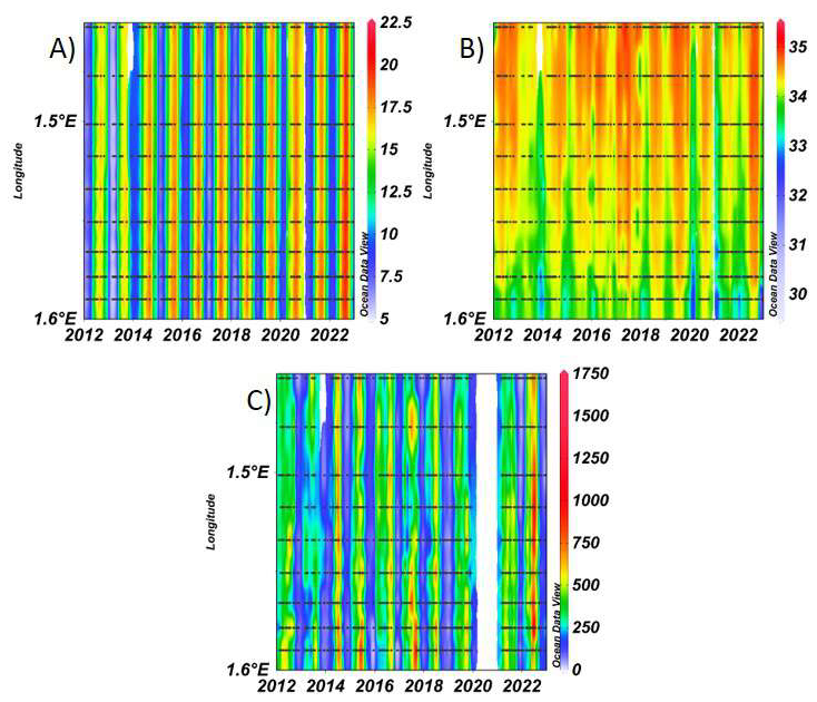
Figure E1 Spatial variability of surface hydrological variables over time: (A) temperature (°C), (B) salinity (PSU) and (C) PAR (µmol s⁻¹ m⁻²) along coastal-offshore DYPHYRAD transects. The figure is organised along a spatial gradient from offshore stations (upper part) to inshore stations (lower part).

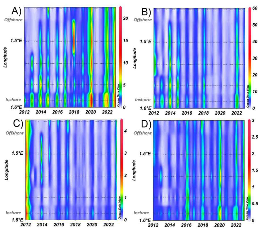
Figure E2 Spatial variability of surface nutrients concentration in µmol L⁻¹ over time (2012–2022): (A) nitrate, (B) nitrite, (C) phosphate and (D) silicate along DYPHYRAD transect.

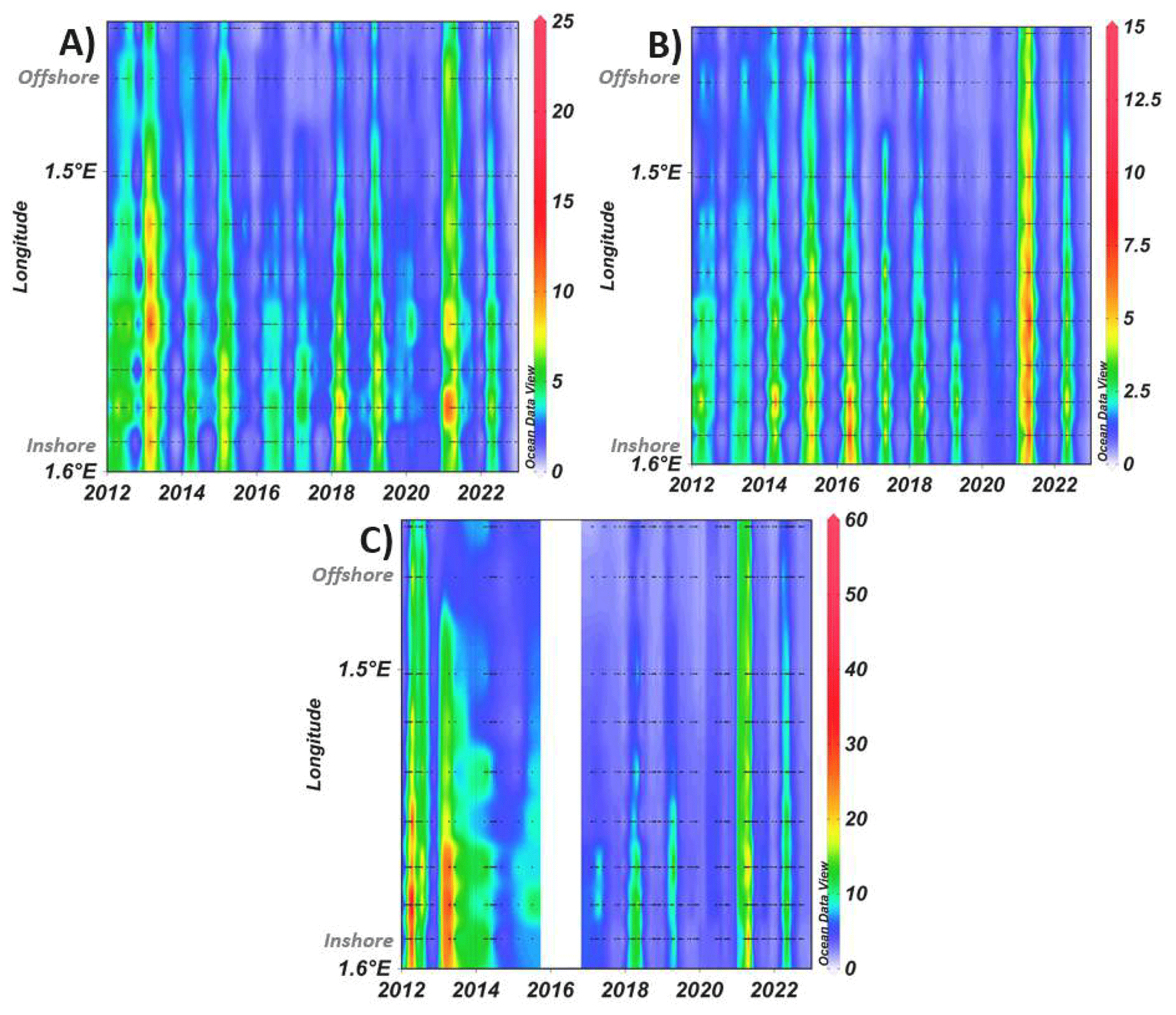
Figure E3 Spatial variability of phytoplankton biomass along the DYPHYRAD transect over time: (A) chlorophyll a (µg L⁻¹), (B) in vivo total chlorophyll a fluorescence (FFU) and (C) FLP Total chlorophyll a equivalents (µg chl-a eq. L⁻¹).

Figure E4 Spatial variability of phytoplankton abundance along the DYPHYRAD trasect, from 2012 to 2022 (cell mL⁻¹): (A) OraPicoProk, (B) RedPico (C) OraNano, (D) RedNano, (E) RedMicro and (F) Total of phytoplancton abundance. The figure is organised along a spatial gradient from offshore stations (upper part) to inshore stations (lower part).