An inter-comparison of inverse models for estimating European CH₄ emissions

Atmospheric inversions are widely used to evaluate and improve inventories of methane (CH₄) emissions across scales from global to local, combining observations with atmospheric transport models. This study uses the dense network of in situ stations of the Integrated Carbon Observation System (ICOS) to explore how well in situ data can constrain European CH₄ emissions. Following the concept of inter-comparison studies of the atmospheric tracer transport model inter-comparison Project (TransCom), a CH₄ inverse inter-comparison modeling study has been performed, focusing on Europe for the period 2006–2018. The aim is to investigate the capability of inverse models to deliver consistent flux estimates at the national scale and evaluate trends in emission inventories, using a detailed dataset of CH₄ emissions described and presented here for first time.

Study participants were asked to perform inverse modelling computations using a common database of a priori CH₄ emissions and in-situ observations as specified in a protocol. The participants submitted their best estimates of CH₄ emissions for the 27 European Union (EU-27) member states, the United Kingdom (UK), Switzerland, and Norway. Results were collected from 9 different inverse modelling systems, using 7 different global and regional transport models. The range of outcomes allows us to assess posterior emission uncertainty, accounting for transport model uncertainty and inversion design decisions, including a priori emission and model-data mismatch uncertainty.

This paper presents inversion results covering 15 years, that are used to investigate the seasonality and trends of CH₄ emissions. The different inversion systems show a range of a posteriori emission adjustments, pointing to factors that should receive further attention in the design of inversions such as optimising background mole fractions. Most inverse models increase the seasonal cycle amplitude, by up to 400 Gg month⁻¹, with the largest adjustments to the a priori emissions in Western and Eastern Europe. This might be due to underestimation of emissions from wetlands during summer or the importance of seasonality in other microbial sources, such as landfills and waste water treatment plants. In Northern Europe, absolute flux adjustments are comparatively small, which could imply that the emission magnitude is relatively well captured by the a priori, though the lower station density could contribute also.

Across Europe, the inverse models yield a similar decreasing trend in CH₄ emissions compared to the a priori emissions (−12.3 % instead of −9.1 %) from 2006 to 2018. While both the a priori and the a posteriori trend for the EU-27 are statistically significant from zero, their difference is not. On a subregional scale, the differences between a posteriori and a priori trends are more statistically significant over regions with more in-situ measurement sites, such as over Western and Southern Europe.

Uncertainties in the a priori anthropogenic emissions, such as in the agriculture sector (cows, manure), or waste sector (microbial CH₄ emissions), but also in the a priori natural emissions, e.g. wetlands, might be responsible for the discrepancies between the a priori and a posteriori emission shift in the trends in Western, Eastern and Southern Europe.

Our results highlight the importance of improving the inversion setup, such as the treatment of lateral boundary conditions and the model representation of measurement sites, to narrow the uncertainty ranges further. The referenced dataset related to the analysis and figures are available at the ICOS portal: https://doi.org/10.18160/KZ63-2NDJ (Ioannidis et al., 2025).

1 Introduction

Methane (CH₄) is the second-most important anthropogenic greenhouse gas (GHG), after carbon dioxide (CO₂), and has a significant contribution to global warming and climate change (IPCC, 2021). In the last two decades, CH₄ emissions increased by 20 %, with mole fractions reaching 1923 parts per billion (ppb) in 2023 (European Environment Agency, 2022; World Meteorological Organization (WMO), 2024). According to a comprehensive recent assessment, annual global CH₄ emissions are around 575 [553–586] Tg yr⁻¹ (Saunois et al., 2025). More specifically, global anthropogenic CH₄ emissions constitute 369 [350–391] Tg yr⁻¹, or around 60 %, of the total CH₄ emissions (Saunois et al., 2025). The largest anthropogenic CH₄ emissions originate from agriculture (e.g., livestock production, rice cultivation), followed by the energy sector (fossil fuel production and use) and waste disposal (IPCC, 2021). However, CH₄ is also emitted from various natural sources (248 [159–369] Tg yr⁻¹, Saunois et al., 2025), with natural wetlands contributing up to 40 % of the total CH₄ emissions (Yusuf et al., 2012; Zhang et al., 2025). The Paris Agreement commits countries to implement mitigation measures to reduce GHG emissions. In addition, 150 countries have signed the Global Methane Pledge, launched in November 2021 at the Conference of the Parties (COP 26) with the aim of reducing global CH₄ emissions by 30 % in 2030 relative to 2020 levels (Global Methane Pledge, 2023).

Anthropogenic emission reporting is based on “bottom-up” inventories, and there are several bottom-up process-based models to estimate natural emissions and sinks. However, these anthropogenic and natural CH₄ emissions have large uncertainties (Brandt et al., 2014; Zavala-Araiza et al., 2015; Deng et al., 2022; Arora et al., 2023). Uncertainties in anthropogenic emissions are caused primarily by uncertain emission factors used in bottom-up inventories (Cheewaphongphan et al., 2019; Solazzo et al., 2021). Some sources of anthropogenic emissions, such as fossil fuel, might also be missing from bottom-up inventories, as shown in a recent study by Yu et al. (2023). Process-based models of natural CH₄ sources and sinks are uncertain for many reasons, including uncertain sensitivities to climatological conditions, small-scale variability that is difficult to scale up, and important processes that may still be missing (Aalto et al., 2025). It is critical for countries to accurately quantify CH₄ emissions, as there is a growing demand from policy makers, reinforced by the Paris Agreement, for efficient methods to reduce CH₄ emissions. Therefore, in addition to these bottom-up emission inventories and process-based models, “top-down” methods have been developed using inverse modeling techniques (Bergamaschi et al., 2018a; Steiner et al., 2024) to bring emission inventories into agreement with atmospheric measurements. The measurements provide independent information on emissions that can be used to evaluate emission inventories, through the use of inverse modelling, in support of the transparency framework of the Paris agreement (World Meteorological Organization, 2016; Calvo Buendia et al., 2019).

The top-down approach, using inversion techniques, yields an optimised “a posteriori” estimate of the emissions. This is done by relating observed atmospheric dry air mole fractions to emissions using an atmospheric transport model, and by minimizing a Bayesian cost function with an inversion algorithm, starting from “a priori” information on emissions and their uncertainties (Jacob, 2007). Different techniques have been developed to solve the inverse problem, such as the Kalman smoother (Bruhwiler et al., 2005), the ensemble Kalman filter (EnKF) (Peters et al., 2005), and the 4D variational inversion (Chevallier et al., 2005). Both EnKF and variational methods have advantages and disadvantages and are widely used today (e.g. Bergamaschi et al., 2022; Saunois et al., 2019; Steiner et al., 2024).

Previous studies used the inverse modeling technique to estimate European CH₄ emissions, using regional (Bergamaschi et al., 2018a, 2022; Petrescu et al., 2023, 2024) or global (Wang et al., 2019; Deng et al., 2022; Petrescu et al., 2023) transport models, based on in situ (e.g. Bergamaschi et al., 2022 or Steiner et al., 2024) and satellite observations (e.g. Bergamaschi et al., 2013, Wang et al., 2019). Bergamaschi et al. (2018b) used different inverse models to estimate European CH₄ emissions for a period of six years (2006–2012). They showed a strong seasonality of CH₄ emissions in Europe due to wetland emissions. In a more recent study, Bergamaschi et al. (2022) focused on 2018 using three high resolution inverse models that showed the a posteriori emissions were higher in Germany and the Benelux than the emissions reported to the United Nations Framework Convention on Climate Change (UNFCCC).

Here, we present a new inverse modelling inter-comparison study, using a detailed dataset of posterior CH₄ emissions, which was prepared as part of the CoCO₂ project and WMO-IG³IS. Using this dataset we aim to evaluate and compare the performance of the nine inverse models participating in the inter-comparison, as well as to estimate European CH₄ emissions over the period 2005–2019. We used a combination of in situ measurement databases, most importantly from the Integrated Carbon Observation System (ICOS) network. This study uses the extended measurement time series to estimate trends in total CH₄ emissions in Europe until 2019. In addition, we try to address the systematic difference in emission seasonality reported by Bergamaschi et al. (2018b). Previous studies have shown large discrepancies between inversion-estimated emissions of CH₄ (Petrescu et al., 2021, 2023). To better understand these differences and to identify some of the potential causes, our experimental protocol (Florentie and Houweling, 2021), presented in Sect. 2, prescribes the a priori emissions and observations to be used. The a priori emissions, the observations used for the different simulation experiments, the validation dataset, the participating models, and information about the modelled output database are described in Sect. 3. The simulations carried out are also described in Sect. 3. The results and a discussion of our findings are presented in Sect. 4. The implications of our findings are presented in Conclusions (Sect. 5).

2 Inversion Protocol

To assess European CH₄ emissions using an ensemble of inversions, a protocol has been formulated by Florentie and Houweling (2021), which the participants are required to use. It closely follows a protocol established in the EU H2020 VERIFY project (https://verify.lsce.ipsl.fr/, last access: 1 January 2020) and utilizes datasets that were collected as part of it. The participants have been instructed to use only atmospheric observations from common datasets (see Sect. 3.1) and a common set of a priori CH₄ emissions (see Sect. 3.2). The protocol also provides climatological radon (²²²Rn) fluxes (Karstens et al., 2015) for simulating ²²²Rn, to assess the performance of the atmospheric transport models that are used. The groups running regional models are required to use initial and lateral boundary conditions from the Copernicus Atmosphere Monitoring Service (CAMS) CH₄ reanalysis v19r1 (Agustí-Panareda et al., 2023), based on assimilated surface observations. Two inversion systems use the Rodenbeck 2-step inversion approach (Rödenbeck et al., 2009), for which consistent baseline conditions are made available as part of the protocol. However, the protocol does not specify the meteorological boundary conditions, the uncertainties to be used for the background mole fractions (concentrations), observations, and a priori emissions, and whether or not to optimise background mole fractions. The participants are requested to provide monthly gridded CH₄ fluxes at 0.25° × 0.25° grid spacing, a priori and a posteriori national total emissions, CH₄ mole fraction time series at the measurement sites and the observation uncertainties. National total emissions are to be provided for at least the European Union (EU-27) countries, the United Kingdom (UK), Norway, and Switzerland. Regional inversions should cover at least the area from 15° W to 35° E and 35 to 70° N. The inversions should cover as many years as possible from 2005 to 2019. In case it is not possible to provide results for the full period, the groups are asked to submit results for a selection of years, chosen to cover the full period as well as possible, including at least the years 2008, 2013 and 2018. This study focuses on total CH₄ emissions, i.e. without sectorial separation of the a posteriori fluxes.

3 Methodology

3.1 Atmospheric measurements

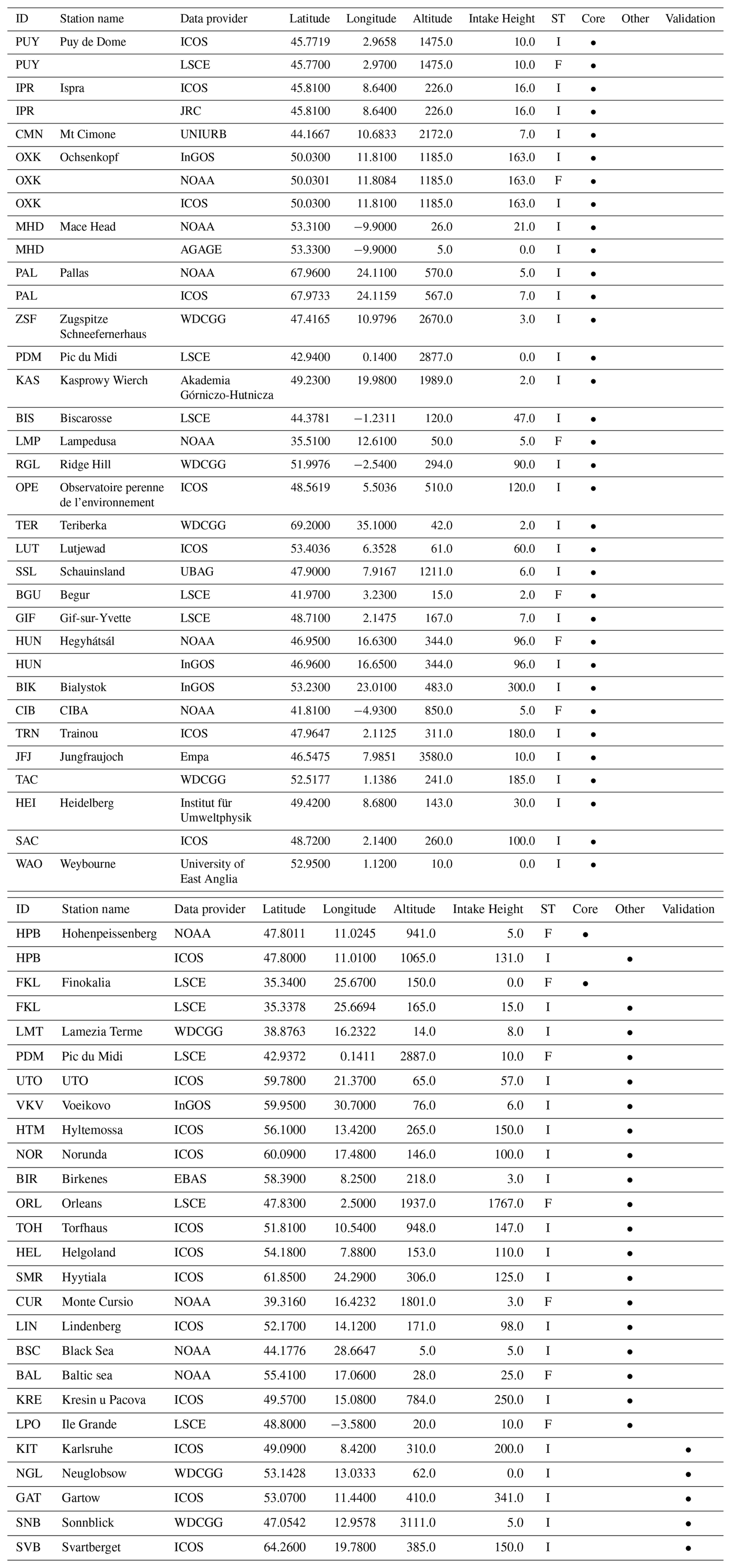
The European monitoring stations used in this study are shown in Fig. 1 and additional information is provided in Table A1. The observations are made available by the Integrated non-CO₂ Greenhouse gas Observing System (InGOS) project (2005–2018) (INGOS, 2018), the National Oceanic and Atmospheric Administration (NOAA) flask sampling network in Europe (2005–2018) (Lan et al., 2023), the Advanced Global Atmospheric Gases Experiment (AGAGE) (Prinn et al., 2018), the ICOS network (ICOS RI, 2021), the World Data Centre for Greenhouse Gases (WDCGG) (, ), the EBAS database hosted by the Norwegian Institute for Air Research, and from the Laboratory for Climate and Environmental Sciences (LSCE). Two sets of observations (“Core” and “Other”) are used in different experiments (see Sect. 3.4), and one set of observations is reserved for validation. The “Core” data set consists of 36 stations, the “Other” data set has 19 stations, while the “Validation” data set includes 5 stations (see Fig. 1).

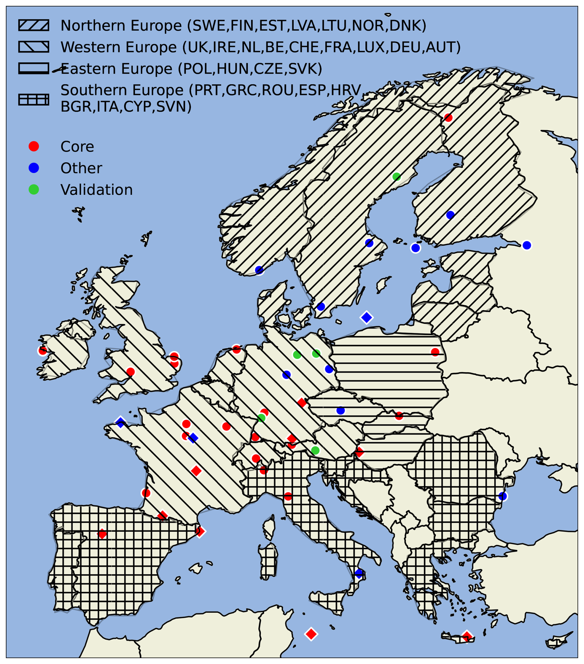
Figure 1 Map showing the locations of in-situ atmospheric monitoring stations used in this study. The map shows the observations used in the different simulations: “Core” is shown as read cycle, and the “Other”, shown as blue cycle, while in green are shown the sites used for validation. Flask stations are shown in diamond. The different hatching patterns highlight the different sub-regions over the domain: “///” is used to define Northern Europe, “\\” for Western Europe, “–” for Eastern Europe and “$++$” for Southern Europe. See text for more details.

The in situ measurements are reported as hourly average dry-air mole fractions (in units of nmol mol⁻¹, abbreviated as ppb), including the standard deviation (measurement uncertainty) which are used in the inversions. In the inversions, only daytime (12:00 to 16:00 local time) and nighttime (00:00 to 04:00 local time) observations are used for surface and mountain sites, respectively.

Figure 1 highlights the sub-regions in Europe used in the analysis of our results. We are using the same region classification as in Bergamaschi et al. (2018a), namely Northern Europe (Sweden, Finland, Estonia, Latvia, Lithuania, Norway and Denmark), Western Europe (United Kingdom, Ireland, Netherlands, Belgium, Luxembourg, France, Germany, Switzerland, and Austria), Eastern Europe (Poland, Czech Republic, Slovakia, and Hungary), and Southern Europe (Portugal, Spain, Italy, Slovenia, Croatia, Cyprus, Greece, Romania, and Bulgaria). The UK and Switzerland are included in Western Europe, but not in the EU-27. Norway is included in Northern Europe, but not in the EU-27.

3.2 A priori emissions

A priori CH₄ emissions used in this study are summarised in Table 1 including information on their spatial and temporal resolutions. The same bottom-up inventories and process-based models for generating natural emissions are used here as in the EU H2020 VERIFY project. More specifically, for anthropogenic CH₄ emissions, the Emissions Database for Global Atmospheric Research (EDGAR) v6.0 is used, which provides emissions for different anthropogenic sectors (Monforti et al., 2021). Year 2018 is repeated for 2019 and 2020. For the anthropogenic emissions, the protocol does not provide information on monthly, daily, or hourly factors to scale the emissions, so all models used temporally constant values. Natural CH₄ emissions from peatlands and mineral soils derived from the JSBACH-HIMMELI model (Petrescu et al., 2023), prepared as part of the EU H2020 CoCO₂ project and do account for seasonality. Climatological CH₄ emissions from inland water, termites, ocean, and geological sinks/sources are used as shown in Table 1. Monthly climatological emissions from ocean and inland water are repeated for all years. The ULB emissions for inland water are provided by the VERIFY project. Global geological emissions are scaled down to 15 Tg yr⁻¹ for this study, as geological emissions have high uncertainties as discussed for example by Thornton et al. (2021). This value is based on a pre-industrial estimate derived from ice core measurements of ${}^{\mathrm{14}}\mathrm{C}{/}^{\mathrm{12}}$C in CH₄ (Petrenko et al., 2017). Finally, the Global Fire Emissions Database (GFED)-4.1s inventory (Randerson et al., 2018) is used for biomass burning emissions. The emissions are provided at their original resolution, and at a regridded resolution of 0.25° × 0.25°, where the total mass has been conserved upon regridding.

Saunois et al. (2019)Weber et al. (2019)Etiope et al. (2019)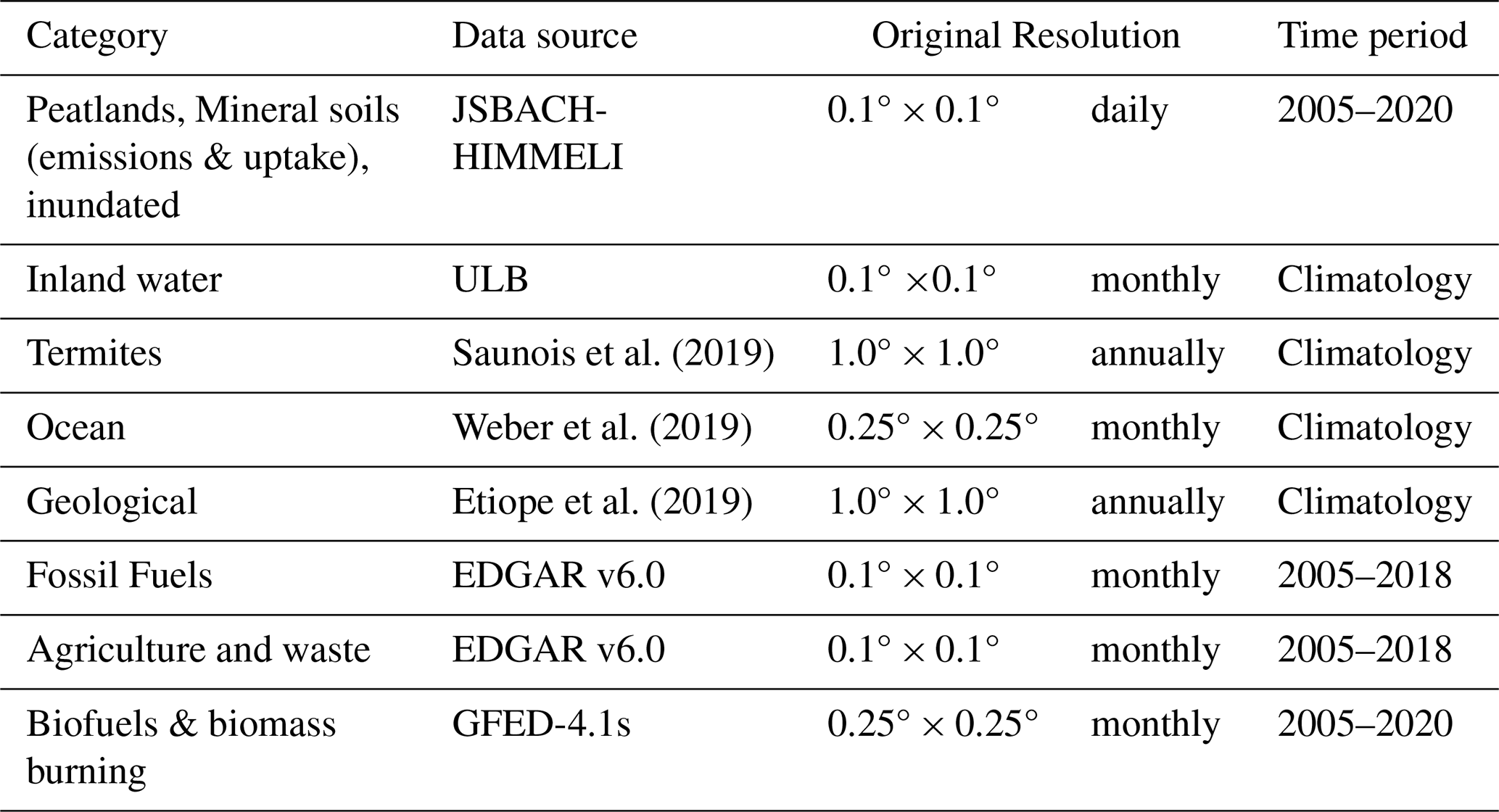

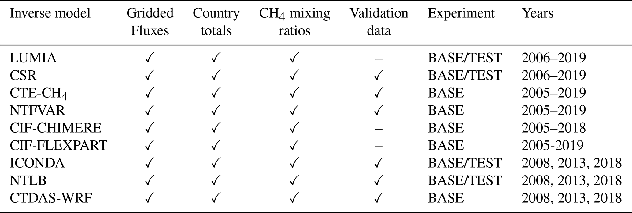
Table 1 A priori CH₄ emissions used in this study.

Table 2 Inversion systems and atmospheric models used in this study.

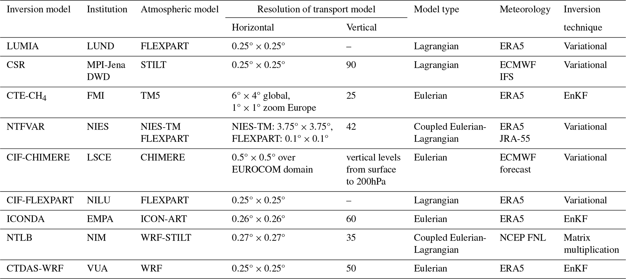
Table 3 Summary of the inversions setups for the different inverse models.

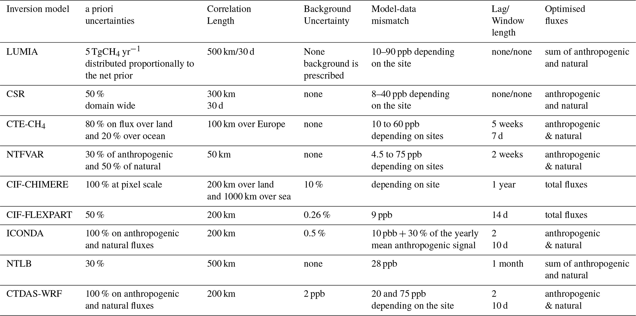
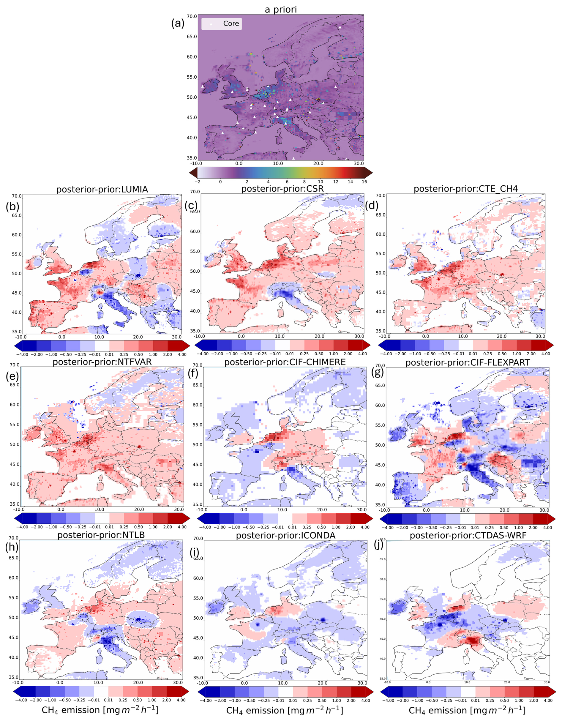
Figure 2 CH₄ emission fluxes, in mg m⁻² h⁻¹, over Europe averaged for the common years 2008, 2013 and 2018, and the BASE simulation. The different panels show (a) the common a priori fluxes, (b–j) the differences between the a posteriori and the a priori fluxes for LUMIA, CSR, CTE-CH₄, NTFVAR, CIF-CHIMERE, CIF-FLEXPART, NTLB, ICONDA, and CTDAS-WRF inverse models, respectively. Panel (a) also shows the location of the observations (“Core”), as white triangles, used in the BASE simulation.

3.3 Atmospheric and inverse models

All inverse models used in this study vary on the type of transport model and resolutions, as well as inversion techniques and uncertainty specifications. The atmospheric and inverse models are listed in Table 2, including information on the resolution of the transport model, model type, background meteorological conditions and inversion technique. Table 3 summarises the inversion setups of the different inverse models. Note that all inverse model results presented here and made publicly available are re-gridded to a common 0.25° × 0.25° resolution. Further details on the atmospheric transport models and inversion techniques that are used can be found in Appendix B.

3.4 Output database

The output dataset consists of CH₄ gridded fluxes, country totals, and CH₄ mole fractions that cover the years from 2006 to 2019, or part of this period, and includes results from 9 different inverse models and two experiments, as defined in the protocol. More specifically, the two experiments are: the baseline inversion (BASE from now on) using “Core” observations (see Table A1), and a test inversion (TEST from now on) in which “Other” observations are used in addition to the “Core” observations (see Table A1). Table 4 summarises the information about the output dataset and simulations performed per inverse model. In the following sections we make use of the dataset to evaluate the performance of the 9 inverse models, as well as to provide insights on the CH₄ emission seasonal cycle and trends in Europe.

Table 4 List of inverse models, available datasets and years for which they provided outputs.

4 Results and Discussion

This section presents the averaged a priori and a posteriori CH₄ fluxes from all the inverse models and for the common years 2008, 2013 and 2018. The performance of the inversions is tested at the measurement sites used in the optimisation as well as the validation observation sites, focusing on the common years. This section also discusses CH₄ emission seasonality and trends over Europe and selected sub-regions, as defined and shown in Sect. 3.1, and for the full common period (2006–2018). The results discussed here are mostly from the BASE run, while results from the TEST run are discussed briefly at the end of each section. Detailed results from the TEST run are shown in the appendices.

4.1 European CH₄ fluxes

4.1.1 BASE results

Figure 2 shows the common a priori (Fig. 2a) CH₄ total (the sum of anthropogenic and natural fluxes) fluxes over Europe, as well as the increments (Fig. 2b–j), calculated as the difference between the a posteriori and a priori fluxes for each model, using results from the BASE run averaged over the common years 2008, 2013, and 2018.

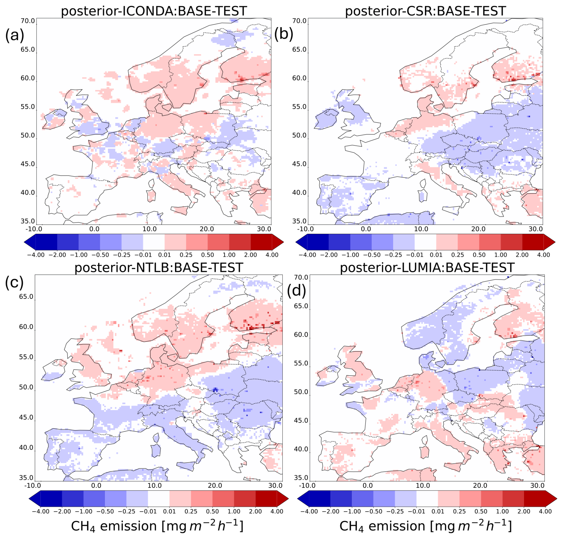
Figure 3 Differences in the a posteriori CH₄ fluxes, in mg m⁻² h⁻¹, between BASE (“Core” observations) and TEST (“Core” and “Other” observations) runs, averaged for the common years 2008, 2013 and 2018. The different panels show results for the different inverse models: (a) ICONDA, (b) CSR, (c) NTLB, and (d) LUMIA.

Figure C1 shows the a posteriori CH₄ fluxes for all the inverse models. The spatial distribution of the a posteriori CH₄ fluxes is similar for all the inverse models and the a priori fluxes over the Benelux region, south of Poland, Finland, the UK and Bretagne. The spatial patterns between the a priori and a posteriori fluxes are similar also over Romania and Po Valley for all inverse models except for CIF-FLEXPART and in the North Sea except for CSR. However, the enhancement or diminishment of the a posteriori compared to the a priori fluxes can be seen in detail by calculating their differences.

Figure 2 shows a large variability in the spatial distribution of flux increments between the different inversion systems. Despite this variability, some common patterns can also be seen. All the inverse models show a strong flux enhancement over the Netherlands. Similarly, a common enhancement is shown over southern UK and Bretagne, although the strength of this enhancement varies among the different inverse models.

All inverse models, except NTFVAR, CTE-CH₄ and CTDAS-WRF, show a systematic reduction over Italy, possibly due to overestimated a priori geological emissions (see Sect. 3.2) that are important in this region (Bergamaschi et al., 2015). The disagreement by NTFVAR, CTE-CH₄ and CTDAS-WRF could be influenced by transport model uncertainties (for example caused by the planetary boundary layer (PBL) structure) in simulating the in-situ observations in that region, notably from Monte Cimone. In CTE-CH₄, geological emissions are not optimised, which may be a reason why this inverse model does not show strong changes in Italy. In northern Europe, where natural CH₄ emissions from wetlands are important, some models show reductions (ICONDA, CTDAS-WRF, CIF-CHIMERE), while others show a small enhancement (CSR, CTE-CH₄) or mixed patterns (NTLB, LUMIA, NTFVAR, CIF-FLEXPART).

Some inverse models (e.g. CSR, CTE-CH₄) show similar spatial patterns over Central Europe, but across all models, the patterns have a large variability in that region. The inverse models show large differences over Ireland and the Iberian Peninsula. As these regions are close to the predominant inflow edge, these differences may be related to the treatment of the western domain boundary condition: regional inverse models, such as LUMIA, CSR, ICONDA, NTLB, CTDAS-WRF, CIF-FLEXPART, use CAMS as lateral boundary condition (or its Rödenbeck variant), some with optimisation, while global inverse models (CTE-CH₄) do not.

Some similarities are found between inverse models that make use of the same transport model or optimisation method. For example, LUMIA and CIF-FLEXPART, which both use FLEXPART, show similarities in Italy, France, northern Europe and part of eastern Europe. However, differences are found over Ireland and the Iberian Peninsula, potentially due to a different treatment of the boundary conditions (see Table 3). The two models that are coupled to the Community Inversion Framework (CIF), CIF-FLEXPART and CIF-CHIMERE, agree with each other, over the Benelux region, Po Valley and parts of central Europe. Furthermore, some inverse models (ICONDA, CTE-CH₄ and CTDAS-WRF) use the CTDAS EnKF for optimisation. However, there is little agreement in the spatial patterns, such as an increase in CH₄ emission over The Netherlands, in these three models. CIF-CHIMERE, CIF-FLEXPART, ICONDA and CTDAS-WRF optimise background conditions, which could explain the similar flux increments over Ireland, the UK, and Spain. However, the global CTE-CH₄ inversion, in which discontinuities at regional domain boundaries do not play a role, shows different patterns in CH₄ emission compared to the other inverse models.

Many other differences between the inverse models may explain the patterns that are found, including differences in meteorological boundary conditions, transport models, inconsistencies in transport with the inversion system used in CAMS, state vector and covariance parameters. To further investigate model uncertainties related to transport, ²²²Rn could be used as a tracer for atmospheric transport. Unfortunately, the number of participants who provided information on ²²²Rn is too low for such an assessment in this inter-comparison.

4.1.2 Influence of number of in-situ stations on a posteriori CH₄ fluxes

Half of the participants submitted results for the BASE and TEST experiments which we used to investigate whether the use of 19 additional stations constrains the CH₄ emissions better. Figure D1 shows the a posteriori fluxes and the differences between the a posteriori and a priori fluxes for the TEST run. In the TEST simulation all the a posteriori fluxes show spatial patterns that are similar to the a priori fluxes, such as over the Benelux region, Po Valley, Romania and southern Poland. All inverse models show overall different patterns, regarding their enhancement or diminishment, between each other over the domain, except ICONDA and NTLB showing similar patterns over Northern Europe, the UK and Ireland. However, all inverse models agree on an increase over the Netherlands/northwest Germany and a negative adjustment of the CH₄ fluxes over Italy. Petrescu et al. (2023) showed regional inversion results over Europe from 2006 to 2017 with negative emission adjustments over Italy, and positive adjustments over the Benelux region for 2 out of the 3 inverse models.

Figure 3 shows the differences between the a posteriori fluxes from the BASE and TEST runs for the inverse models with results for both runs. In the TEST run, there are more stations in central and northern Europe, as well as in Italy, Greece, and Romania. All inverse models show different BASE vs. TEST patterns, but there are clusters of inverse models showing similar patterns over specific regions. For example, ICONDA and LUMIA (Fig. 3a,d) show higher emissions in the TEST simulation over south Eastern Europe, where there is only one new station (in Romania) compared to the BASE simulation. On the other hand, three inverse models agree (Fig. 3a, b, c) on increased CH₄ emissions over Germany, Denmark, and southern Sweden and Norway, which are in the footprint of stations in the “Other” list, but not in the “Core” list. The comparison between the BASE and TEST simulations shows overall similar spatial patterns for most of the inverse models (compare Figs. 2 and D1), indicating a moderate sensitivity to the network geometry.

4.2 Evaluation of inverse models

The a priori and a posteriori modelled CH₄ mole fractions are evaluated against the observations used in the inversion and against independent measurements. Here we present summary statistics across all stations, comparing the different inverse models for the common years.

4.2.1 Optimised stations

Figure 4 shows the averaged root mean square error (RMSE), mean bias, and correlation coefficients between the a priori and a posteriori modelled CH₄ mole fractions and the observations used in the optimisation set-ups (“Core” list in Table A1). The statistical metrics are shown per inverse model and they are calculated per station and then averaged over the three common years.

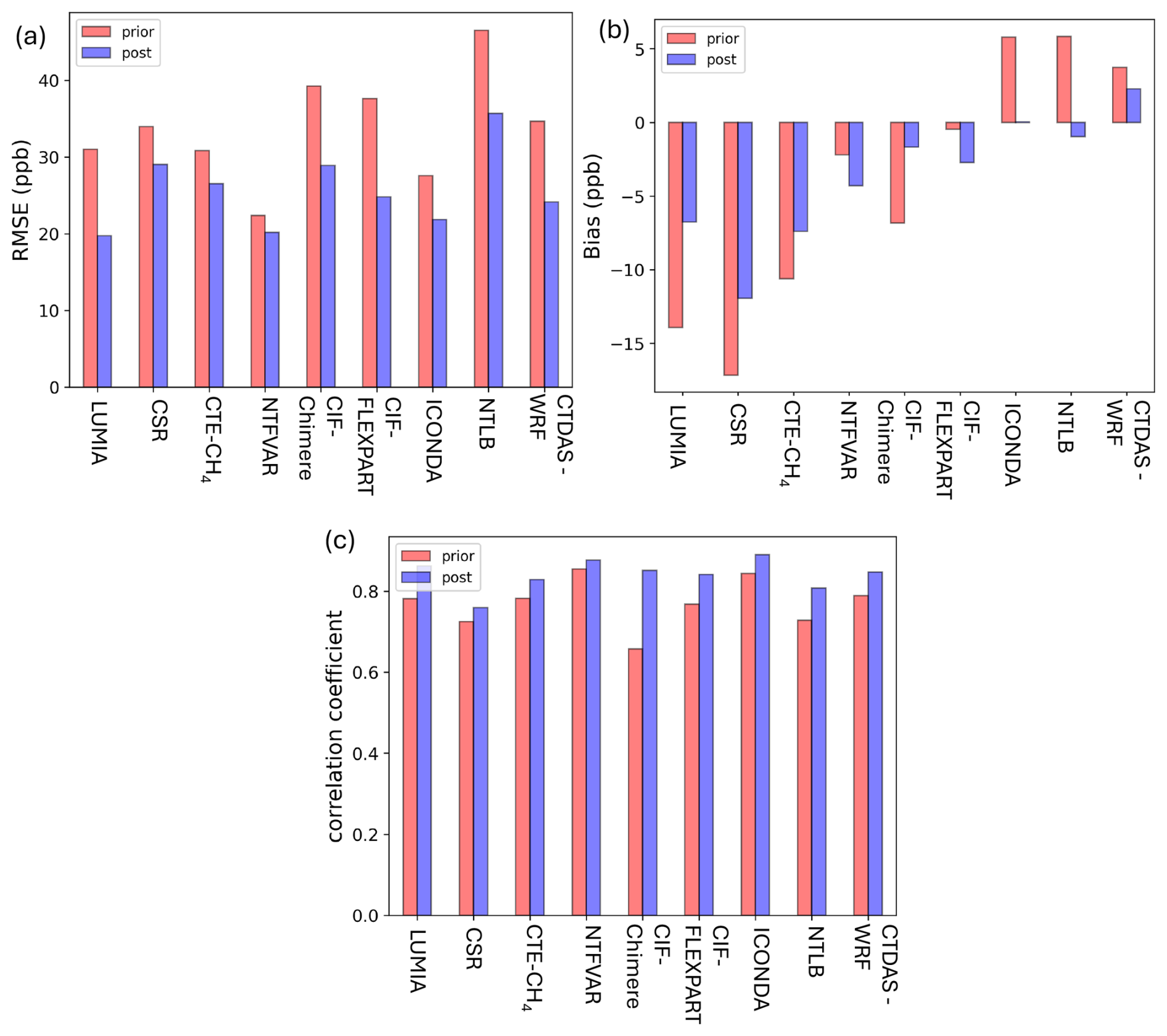
Figure 4 Evaluation of the a priori and a posteriori modelled CH₄ mole fractions, against all available observations used in the optimisation and averaged for the common years 2008, 2013 and 2018 (“Core” list, as shown in Table A1), and for the BASE simulation. (a) shows mean RMSE in ppb, (b) shows mean bias in ppb, and (c) shows correlation coefficient, for all inverse models. The pink and blue bars represent, respectively, a priori and a posteriori CH₄ mole fractions.

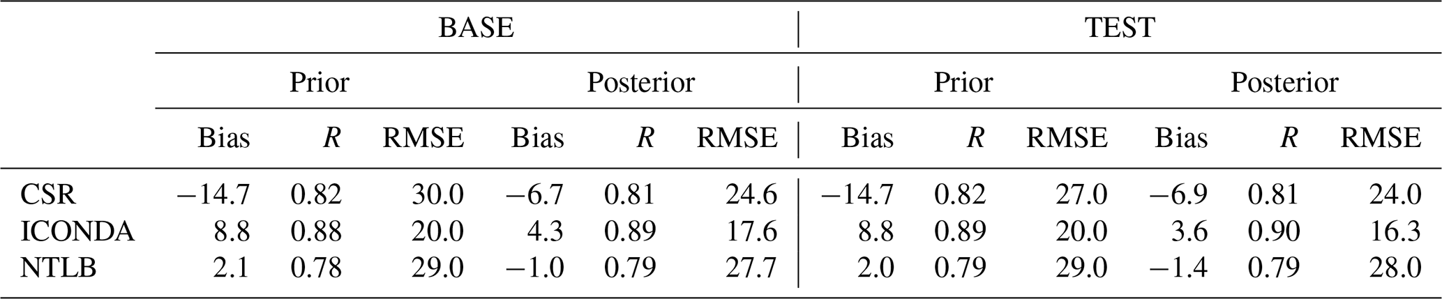
Table 5 Statistical summary for the inverse models which provided CH₄ mole fractions for the optimised stations from both simulations. Bias and RMSE are expressed in ppb. R is Correlation coefficient. The statistics are for the common years.

As expected, a posteriori CH₄ mole fractions show better agreement with the observations than the a priori, with reduced RMSEs and biases, with ICONDA and NTLB having the smallest biases. Note that CIF-FLEXPART and NTFVAR show slightly higher a posteriori biases, compared to the a priori, while the a posteriori RMSE is reduced, with an averaged (over the common years) observation uncertainty of 43 ppb. The results in Fig. 4a show a correlation between RMSE and model resolution. ICONDA, LUMIA and NTFVAR (regional inverse models) show the lowest RMSE. All a posteriori results show improved correlation coefficients, higher than 0.8. Table 5 summarises the statistics for the inverse models that provide CH₄ mole fractions for the optimised stations in the BASE and TEST simulations. The use of more stations results in improved statistics for all inverse models in general. For example, RMSE is further improved for all inverse models in the TEST simulation, with comparable correlation coefficients between the two runs. ICONDA and LUMIA performed better than the other two inverse models.

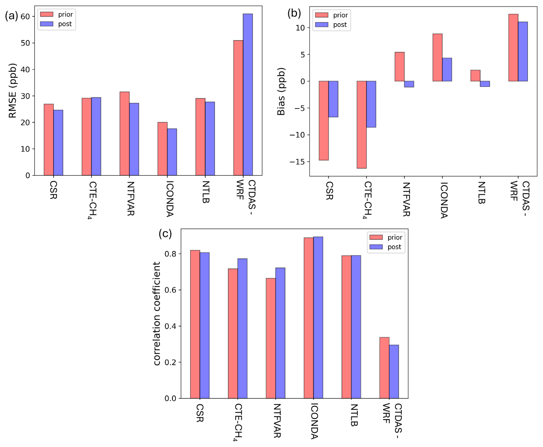
Figure 5 Validation of the a priori and a posteriori CH₄ mole fractions against the independent observations for the common years 2008, 2013 and 2018 (Validation list, as shown in Table A1), and for the BASE simulation. (a) shows mean RMSE in ppb, (b) shows mean bias in ppb, and (c) shows correlation coefficient, for six inverse models. Pink color shows the validation against the a priori CH₄ mole fractions, while the blue shows the validation against the a posteriori CH₄ mole fractions.

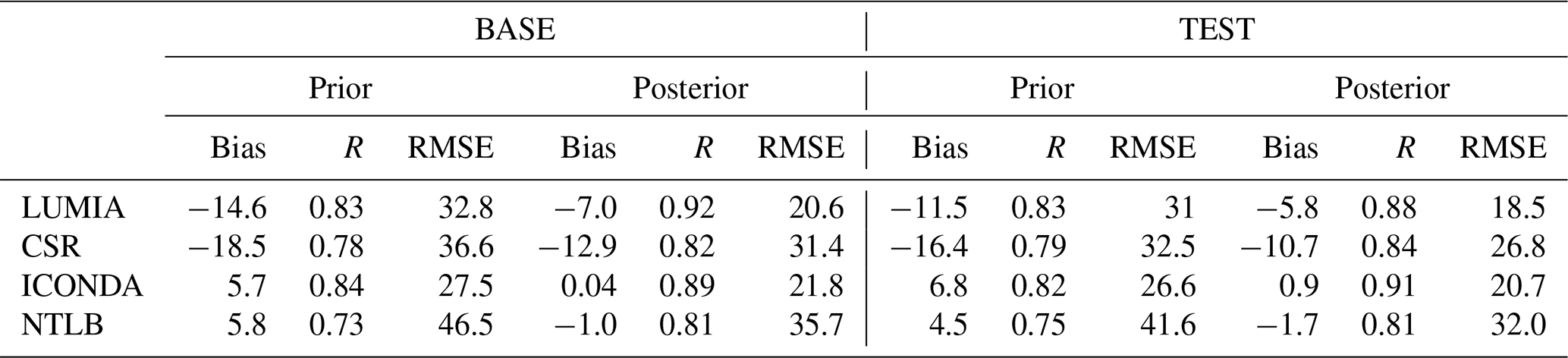
Table 6 Statistical summary for the inverse models which provided CH₄ mole fractions for the validation stations from both simulations. Bias and RMSE are expressed in ppb. R is Correlation coefficient. The statistics are for the common years.

4.2.2 Validation stations

Figure 5 shows the averaged RMSE, mean bias, and correlation coefficients between the a priori, a posteriori modelled CH₄ mole fractions, and the independent observations (Validation list, as shown in Table A1) for the BASE simulation. Bear in mind that not all inverse models provided results for the validation stations (see the “Validation data” part in Table 4). Averaging over all stations, the RMSEs (Fig. 5a) decreased for almost all inverse models, with ICONDA having the smallest RMSEs. Fig. 5b, c also show improved a posteriori results with low biases and correlation coefficients higher than 0.6 respectively for four out of six inverse models. Two of the inverse models that submitted results for the validation stations simulated these observations considerably less well than the observations that were optimised: CSR (Fig. 5c) and CTDAS-WRF (Fig. 5a, c),where the latter shows the poorest performance in this metric among all inverse models, despite using a similar inversion setup to an outperforming inverse model, such as ICONDA (see Table 3). The poorer overall performance of CTDAS-WRF is driven by big discrepancies with the observations during winter and fall (not shown here). Hence, we assume that this could be due to errors in simulating the shallow boundary layer, which is a common transport model error (Gerbig et al., 2008; Deng et al., 2017; Lehner and Rotach, 2018). Errors in the modeling of atmospheric transport, such as advection schemes, sub-grid scale parameterizations, and horizontal and vertical resolutions, could also be responsible for these discrepancies, as has been reported by previous studies, such as Locatelli et al. (2013). Complex terrain, e.g. mountainous sites, could also introduce biases in the results, as it is difficult to simulate inflow in and around mountains (e.g. Al Oqaily et al., 2025). The performance of CTDAS-WRF with respect to the stations that were optimized for is much better (compare Figs. 4 and 5), which suggests that the poor performance with respect to the validation stations could be due to overfitting. However, on average, the fit to the optimized stations does not improve more in the CTDAS-WRF inversion than some other models (Fig. 4), suggesting that the weight of the observations in the inversion was not considerably larger than in the other models. Overfitting could still play a role for individual stations, but further analysis is needed. Finally, the statistics presented here are averaged using all the stations for the common years. Therefore it is possible that the statistics are driven by one of the stations. Table 6 summarises the statistics for the inverse models that provide CH₄ mole fractions for the validation stations for both the BASE and TEST simulations. The use of more stations in the TEST simulation resulted in better agreement between the modelled and the observed molar fractions for all inverse models, as shown by the lower RMSEs for all models. ICONDA performs better than the other two inverse models with a lower bias and a higher correlation coefficient in both simulations. For details regarding ICONDA's development and detailed testing for European CH₄ inversions please refer to Steiner et al. (2024).

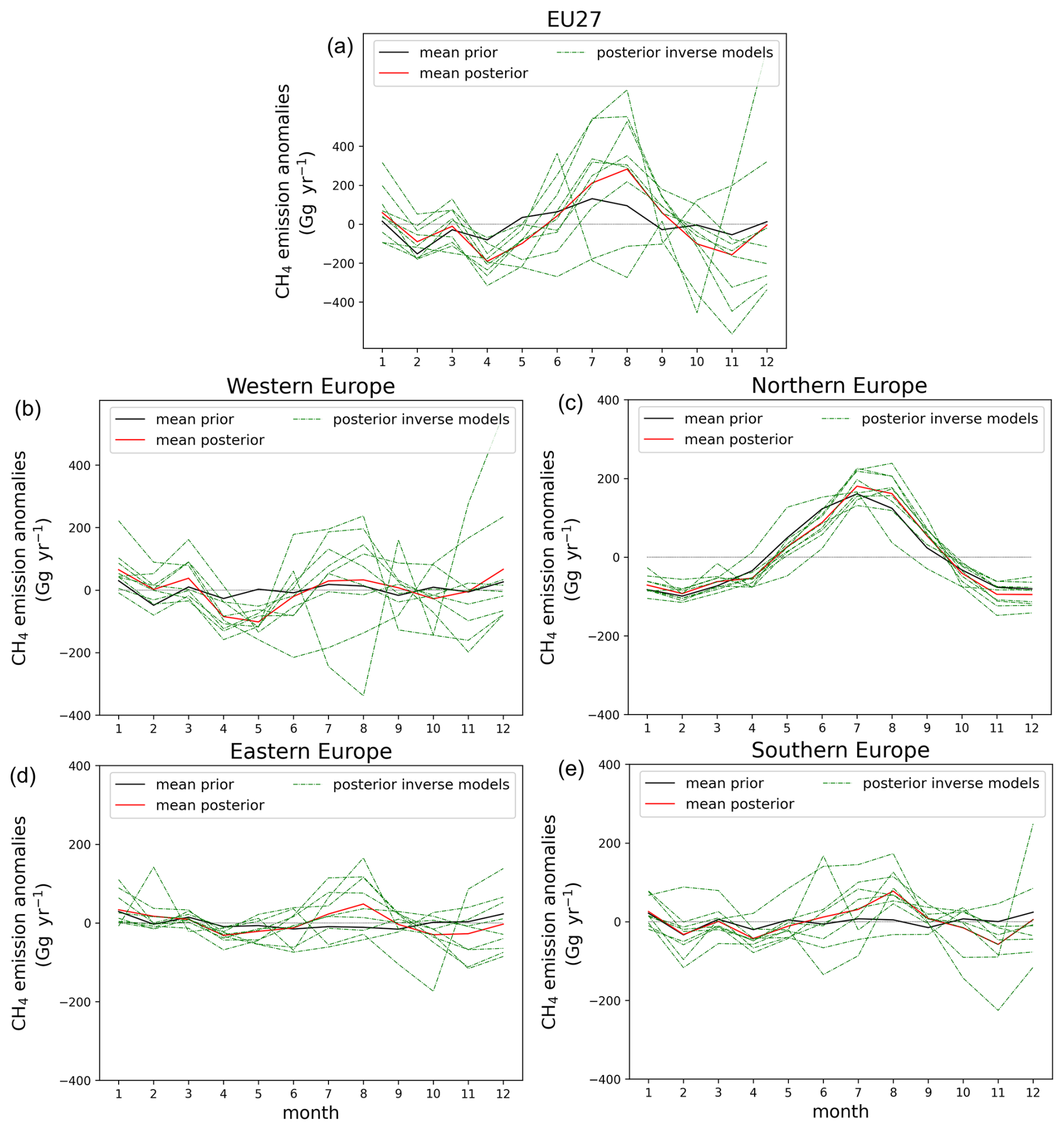
Figure 6 Seasonal cycle of CH₄ emission anomalies, in Gg month⁻¹, for 2006–2018. The black solid line shows the mean a priori emissions, while the red line shows the mean a posteriori emissions. The green lines show the a posteriori results from the different inverse models. This figure shows the seasonal cycle for (a) EU-27, (b) Western Europe, (c) Northern Europe, (d) Eastern Europe and (e) Southern Europe, based on the BASE simulation.

The reductions in RMSE and bias from a priori to a posteriori is less for independent sites than for optimised sites (Fig. 4). Some loss in performance is expected due to uncertainties in atmospheric transport models, and limitations in the coverage of the measurements that are used in the optimisation. This is also reflected in the correlation coefficients which barely improve, as the measurement variability is largely determined by the meteorology, which is not optimised.

4.3 Seasonal cycle

Figure 6 shows the seasonal cycle of total CH₄ emission anomalies for EU-27 (Fig. 6a), Western, Northern, Eastern and Southern Europe (Fig. 6b–e), using results from the BASE run. See Fig. 1 (Sect. 3.1) for the sub-regions definition. The seasonality is estimated by subtracting the annual mean of each year from the monthly values of that year. Here we treat the different inverse model results as an ensemble consisting of 9 BASE runs (see Fig. 6) and 4 TEST runs (see Appendix E and Fig. E1), as shown in Table 4. The average over all models is also shown. For the EU-27, the a posteriori CH₄ emissions show an enhanced seasonal cycle compared to the a priori, with a maximum in July/August and a minimum in March/April and November/December. Although the models generally follow the same pattern, there is a considerable spread in the individual inverse models, especially during summer and winter months. To further investigate the origin of this signal in the a posteriori CH₄ emissions, we split the EU-27 in four sub-regions.

A priori CH₄ emissions show a very small seasonal cycle in all sub-regions (Fig. 6b, d, e), except for Northern Europe (Fig. 6c). In Northern Europe, a priori CH₄ emissions are enhanced during the summer (Fig. 6c), due to the contribution of natural wetland emissions, as shown in previous studies (Bergamaschi et al., 2018b). We expect the influence of the hydroxyl radical (•OH) on CH₄ to be small over Europe (Zhao et al., 2020). East et al. (2024) attributed wetland emissions as the primary driver of CH₄ seasonality during summer in the northern hemisphere, while CH₄ sinks, such as •OH, are unlikely to play a significant role. A posteriori CH₄ emissions follow the a priori seasonality, however, the signal is slightly more enhanced during summer and extends longer into autumn. By using the JSBACH-HIMMELI model as the only a priori estimate for natural emissions, we might indeed underestimate total emissions over Northern Europe during summer, because it does not account for emissions from rivers and lakes (Tenkanen et al., 2025). Though JSBACH-HIMMELI also does not explicitly resolve coastal wetland emissions. Recent studies, such as by Aalto et al. (2025), have demonstrated JSBACH-HIMMELI's limitations in producing accurate CH₄ wetland emissions, due to uncertainties in processes, for example, linked to temperature and precipitation. Although temperature and precipitation are important drivers, studies suggest that CH₄ emissions are more sensitive to inundation (Gerlein-Safdi et al., 2021). Inundation, after snow-melt, could induce large CH₄ emissions in spring. Inundation in JSBACH-HIMMELI is taken as prescribed from satellite data (WAD2M, Zhang et al., 2021) and CH₄ emissions from inundated lands are calculated using the approach by Spahni et al. (2011). However, bottom-up process-based models, such as JSBACH-HIMMELI, have limitations combining emissions from different types of land, which might result in limitations in the total wetland CH₄ emissions.

In other sub-regions, the model-average of a posteriori CH₄ emissions show a slightly enhanced seasonality compared to the a priori. An increase was expected since the anthropogenic component of the prior emissions had no seasonal cycle in our protocol. A posteriori emissions show stronger emissions during summer, with a peak in August, in Southern Europe (Fig. 6e) than the a priori. Similar seasonal adjustments are found in Eastern Europe (Fig. 6d), although slightly less strong than in Southern Europe, with a smaller spread of the ensemble members. We speculate that factors contributing to a summer maximum in these regions could be enhanced energy use due to air conditioning (Dong et al., 2021) and microbial sources such as CH₄ emissions from land fills and waste water, which we assume respond to warmer temperatures with higher CH₄ emissions (Hu et al., 2023). Neither factor would be accounted for in temporally resolved bottom-up data for these regions: time profiles for power use available in the literature are not region-specific and feature a maximum of energy use in winter (e.g. Kuenen et al., 2014), and to our knowledge up to date time profiles are not available for waste treatment (Guevara et al., 2021). Therefore, while including a seasonal cycle in the anthropogenic prior emissions may have improved the prior estimate in other regions, it could have increased the discrepancy between prior and posterior seasonal cycles in Southern and Eastern Europe. Note that both regions are not well covered by the observation network and the sites in the center of those regions may drive the adjustments in the a posteriori results.

In Western Europe, the seasonality in inversion-optimised CH₄ emissions shows a double maximum in winter and summer (Fig. 6b). The spread of the ensemble members (the different inverse models) is bigger, however, in Western Europe than in the other sub-regions, and seems to drive the spread shown in EU-27 (Fig. 6a). A missing contribution from fossil fuel use (e.g. domestic heating) to the a priori seasonal cycle might explain the difference between the a posteriori and a priori winter peak in January extending into February and March. Recent studies point to CH₄ leaks from oil and gas pipelines in Western European cities, which might be missing in bottom-up inventories (Maazallahi et al., 2020; Defratyka et al., 2021; Dowd et al., 2024). However, only small seasonal variations have been found for natural gas distribution systems (McKain et al., 2015; Wong et al., 2016), so this processing is unlikely to explain the different seasonalities in the a posteriori emissions compared to the a priori emissions.

Uncertainties in agricultural emissions from livestock and manure management might also influence emission seasonality (Solazzo et al., 2021; Petrescu et al., 2021; Ghassemi Nejad et al., 2024). Recent studies show that emissions from storage and treatment of manure are temperature dependent, and exhibit seasonal variations (Cárdenas et al., 2021; Zhang et al., 2021; Ólafsdóttir et al., 2023). Other studies have reported significant variations in CH₄ emissions from dairy cows, due to the lactation periods of cows (Ulyatt et al., 2002). Increased agricultural emissions during summer combined with increased fossil fuel emissions during winter could explain the double peaked seasonal variability in the a posteriori CH₄ emissions in Western Europe, as well as seasonal emission adjustments in other sub regions. Conducting source-resolved posterior analyses in future studies, for example using isotopic measurements, would facilitate a more precise quantification of contributions from agricultural and fossil fuel sources.

Two inverse models exhibit abnormal seasonality: CTDAS-WRF in Western Europe (August-December) and NTLB in Southern Europe (from August to November), despite the latter performing better than CTDAS-WRF when comparing against the independent observations (Fig. 5). Although CTDAS-WRF and NTLB use a different inversion setup as shown in Table 3 and therefore it is difficult to point out the cause of these discrepancies, both inverse models are driven by the same transport model (WRF). It is known in the literature that WRF has difficulties simulating realistic mixing, as mentioned earlier in Sect. 4.2, and BL and strongly depends on the parametrisation used (e.g. Banks and Baldasano, 2016). We estimated the seasonal cycle without those two inverse models (not shown here). When excluding results from CTDAS-WRF and NTLB, the seasonal patterns remain largely consistent across Southern, Northern, Western and Eastern Europe, with minimal changes to the overall seasonality.

The TEST run (see in Appendix E) shows seasonal emission adjustments that are similar to the BASE run, namely a strong seasonal cycle in the a posteriori fluxes in EU-27 (Fig. E1a), as well as in Western and Northern Europe (Fig. E1b and E1c respectively). Interesting patterns are shown in Southern and Eastern Europe, namely a stronger variability during summer and winter compared to the BASE run (Fig. 6d). More stations are available in the TEST run over Western and Southern Europe, compared to the BASE run. Therefore, more information is available to constrain the a priori emissions, which might explain the increased seasonal emission adjustments. The reasons discussed earlier could be responsible for the discrepancies between a priori and a posteriori results.

4.4 CH₄ emission trends

According to the European Environment Agency (European Environment Agency, 2022), regulations at the European level, following the Kyoto protocol and the Paris agreement, have resulted in a decrease in CH₄ anthropogenic emissions from the energy sector, including fugitive emissions from oil, coal and natural gas, as well as the agriculture and waste sectors, since the early 1990s. Previous inverse modelling inter-comparison studies, such as by Bergamaschi et al. (2018b), did not discuss trends in CH₄ emissions in detail, as they focused on a shorter time period (2006 to 2012). Nevertheless, Bergamaschi et al. (2018b) reported a negative trend in CH₄ emissions for EU-28 (including the UK). Petrescu et al. (2021, 2023) compared top-down and bottom-up estimations for several years, but provided trends only for the a priori emissions.

Table 7 A priori and a posteriori anomaly trends over the years 2006 to 2018 for EU-27 and the four sub-regions. p-value is given for mean a priori, mean a posteriori trend and for the difference between the mean a posteriori and mean a priori trend. These results are based on the BASE simulation. See text for more information.

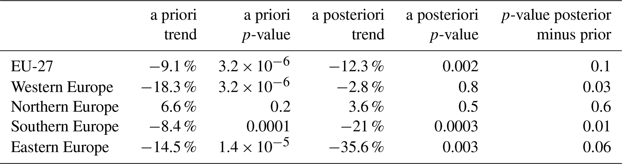
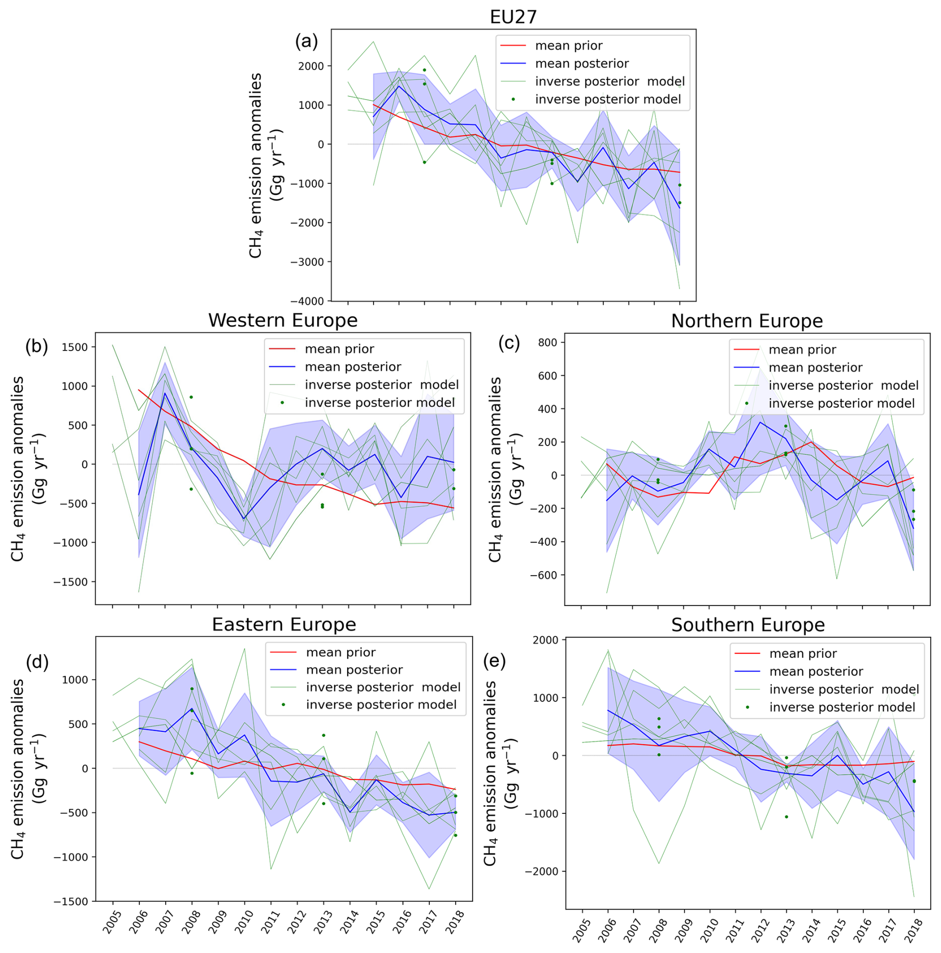
Figure 7 Total CH₄ emission anomaly trends, in Gg yr⁻¹, over (a) EU-27, (b) Western Europe, (c) Northern Europe, (d) Southern Europe and (e) Eastern Europe and over the common long period (2006–2018), based on the BASE simulation. The red line shows the mean a priori model results, the blue line shows the mean a posteriori results, while the green lines and dots show the a posteriori model outputs. The horizontal gray line shows the reference line at y=0. The blue shade shows the emissions' uncertainty, which is estimated using the standard deviation of the ensemble of models. Note the scales are different.

Here we present a detailed analysis of CH₄ emission anomaly trends over Europe and sub-regions (Fig. 7), as defined earlier, including the common years from all the inverse models provided results for a long time period (see Table 4). Standarised anomalies are estimated first by inverse model and then the results are averaged to get the mean posterior anomaly trends. The results based on the BASE run are shown here. The trends from the TEST run are not shown here since only two models submitted results for all the years. Table 7 summarises the a priori and a posteriori trends for EU-27 and per sub-region, and also shows whether the trends and the difference between the a posteriori and a priori trend are statistically significant, as indicated by the p-value, computed using the Mann-Kendall test (Mann, 1945; Kendall, 1948; Gilbert, 1987). We consider results to be statistically significant when the p-value is less than 0.05.

The EDGAR inventory used for the a priori anthropogenic emissions in this study indicates a decrease in CH₄ emissions over Europe as well as all our sub-regions except Northern Europe (Table 7), where the prior shows no significant trend. More specifically, a priori CH₄ emissions show a negative trend (−9.1 % or −0.7 % yr⁻¹) in EU-27 (Fig. 7a), while the decrease is stronger (−18.3 % or −1.3 % yr⁻¹) in Western Europe (Fig. 7b) and in Eastern Europe (−14.5 % or −1.04 % yr⁻¹) (Fig. 7d). The a priori trends are statistically significant for EU-27 and these three sub-regions, whereas no statistically significant trend is present in the prior emissions for Northern Europe (Fig. 7c).

The inverse model outputs are treated here as ensemble members and the trend based on the mean a posteriori emissions is analysed. The trends of averaged a posteriori results agree with the prior (i.e., are not statistically significantly different) in the EU-27, where they show a similarly strong negative trend (−12.3 % or −0.9 % yr⁻¹), and in Northern Europe, where no statistically significant trend is detected (+3.6 % or +0.3 % yr⁻¹). By contrast, the trends of the mean a posteriori emissions in Western, Eastern and Southern Europe differ significantly from the trends of the respective a priori emissions. The emission reduction trends in both Southern (−21 % or −1.5 % yr⁻¹, Fig. 7e) and Eastern (−35.6 % or −2.5 % yr⁻¹, Fig. 7d) Europe are significantly stronger than in the a priori. The stronger decline on CH₄ emissions over Southern and Eastern Europe compared to the a priori could be driven from the observations used to constrain the a priori emissions. Follow up studies could further explore what drives the emission trends (e.g. in-situ stations, background optimisation) in the European boundaries. The opposite applies to Western Europe: while the a priori emissions show the above-mentioned significant emission decrease (−18.3 % or −1.3 % yr⁻¹), the a posteriori emissions saw a small decrease (−2.8 % or 0.2 % yr⁻¹) which is not a significant trend. We note that the period with the strongest emission reductions in the a prior in Western Europe, 2006–2011, is characterized by much higher interannual variability than in the other periods and regions, with relatively small uncertainty among the models.

Overall, the inversions retrieve a similar trend as the a priori over the aggregated EU-27 region, but shifts emission reductions in the a priori from Western Europe to Eastern and Southern Europe.

5 Code and data availability

The output database has been prepared in network Common Data Form (NetCDF) and comma-separated values (csv) format and are available at the ICOS portal: https://doi.org/10.18160/KZ63-2NDJ (Ioannidis et al., 2025). The input data, observations and emissions, used in this study are included in the ICOS portal. The protocol can be found at https://doi.org/10.5281/zenodo.15082281 (Florentie and Houweling, 2021). All the inverse and transport models are publicly available online.

6 Conclusions

A new inverse modelling inter-comparison has been presented to study European CH₄ emissions, organised as part of the CoCO₂ project and WMO-IG³IS. The participating groups submitted inverse model outputs of a posteriori CH₄ emissions, and a priori and a posteriori CH₄ mole fractions over Europe covering the period from 2005 to 2019. The inversion setups follow an experimental protocol specifying common a priori CH₄ emissions and in-situ measurements to be used in two inversions, using different sets of in-situ stations (BASE and TEST runs). This resulted in 9 model submissions for the BASE run and 4 for the TEST run, which have been used to analyse mean emission adjustments, emission seasonality, and trends during the study period.

The inverse models use different atmospheric transport models, operating at different resolutions, and inversion techniques, which differ in model-data mismatch and a priori flux uncertainties. The optimised emissions adjustments from the a priori show significant spatial variations across the European domain with differences between the inverse models that largely persist in time. We believe that some of these differences could be due to known critical issues in regional inverse transport modelling, such as the sensitivity to the treatment of domain boundaries, atmospheric transport uncertainty (such as representation of mountain sites due to uncertainties in the PBL structure) and the relative weight of the data and a priori fluxes. Despite these differences, the inverse model outputs also show common spatial patterns in a posteriori emission adjustments, such as a systematic enhancement over The Netherlands and northern Germany, over southern UK and Bretagne. Most models agree on emissions reduction over Italy and Belgium. To test inversion performance, the a priori and a posteriori CH₄ mole fractions have been evaluated against measurements that are used for optimisation and validation. The optimisation decreased the RMSEs and biases for all inverse models from a priori values ranging between 21 and 45 ppb RMSE and −17 to 5 ppb bias, to a posteriori RMSEs ranging between 20 and 33 ppb and biases of −12 to 2 ppb, for sites used in the optimisation. RMSEs and biases also decreased for all but one model compared to independent measurements, from a priori values ranging between 19 and 50 ppb RMSE and −16 to 13 ppb bias, to a posteriori values range between 18 and 60 ppb RMSE, and −8 to 11 ppb bias. Modelled a posteriori CH₄ mole fractions also improved in the TEST simulation, compared to the a priori. However, the use of more stations did not lead to better results against the independent stations compared to the BASE run. ICONDA and LUMIA are the inverse models that perform better than the rest in this study based on the above analysis.

The analysis of optimised CH₄ emissions reveals a stronger seasonal cycle, by up to 220 Gg month⁻¹ on average, in the a posteriori CH₄ emissions compared with the a priori (up to 100 Gg month⁻¹) integrated over the EU-27, peaking in summer. After splitting up the EU-27 into sub-regions, a stronger seasonality is found in the multi-model mean a posteriori than in a priori emissions across the European domain, albeit with large inter-model differences. However, the shape of the a posteriori seasonal cycle varies between Western Europe, with emission maxima during winter and summer, and Northern, Southern and Eastern Europe, where emissions peak during summer. The seasonal cycle of the a posteriori CH₄ emissions is stronger than the a priori, driven entirely by the observations, as we didn't impose a seasonal cycle on the a priori emissions. Further investigation could help to quantify the uncertainty imposed on a priori emissions due to the use of temporal profiles. Natural CH₄ emissions from wetlands or wet mineral soil could be underestimated, up to 20 %, in the JSBACH-HIMMELI process-based model (Aalto et al., 2025; Ying et al., 2025), although Northern Europe has only a relatively minor contribution to the EU-27 seasonal cycle adjustment. Missing seasonality in the anthropogenic emission sectors, such as fossil fuel (e.g. energy sector due to intense heating in winter or due to intense use of air conditioning in summer), waste treatment (livestock waste, landfills, waste water plants) could play a role also on top-down estimations (Tenkanen et al., 2025), but needs further investigation.

Compared with previous inversion inter-comparison studies, we were able to extend the inversion time window with additional years of measurements, allowing us to study a priori and a posteriori trends in CH₄ emissions. According to the a priori CH₄ emissions inventory the emissions in the EU-27 decreased by 9.1 % between 2005 and 2019, while the inversion results (−12.3 %) agree within uncertainties. Analyzing this result by sub-region, the inversions shift an emission decrease in Western Europe that is present in the a priori to Eastern and Southern Europe. The inversion results for Western Europe until 2011, i.e. the period of biggest emission reductions in the a priori, exhibit bigger a posteriori emissions inter-annual variations compared to any other period or region in our analysis.

This is the first inversion inter-comparison study of national CH₄ emissions for Europe spanning 15 years. Our results highlight the importance of optimised lateral boundary conditions in regional inversions and accurate representations of the optimised stations by the atmospheric transport models that are used. Most of the participating inversion systems are still under development for long-term applications. Including background mole fractions optimization within the inversion framework enhances the agreement between posterior modelled and observed mole fractions, particularly in regions close to the boundaries of the modeling domain and minimises uncertainties due to biases on long-way transport (Steiner et al., 2024). More specifically, the choice of optimising background mole fractions seems to be important for constraining long-range transport or inconsistencies caused by the lateral boundary conditions. Future projects could investigate in detail the role of optimising background mole fractions in the inversions with detailed sensitivity runs. Follow-up inter-comparison studies are in preparation in the on-going European projects Attributing and Verifying European and National Greenhouse Gas and Aerosol Emissions and Reconciliation with Statistical Bottom-up Estimates (AVENGERS), Verifying Emissions of Climate Forcers (EYE-CLIMA) and Process Attribution of Regional Emissions (PARIS) for which this study can serve as a reference. Detailed protocols with prescribed prior emissions, common observations to be used for optimisation and validation, and lateral boundary conditions, as has been done in this study, can help to narrow down inter-model discrepancies. The use of common meteorological boundary conditions in a subset of inverse models, as in Munassar et al. (2023), could be explored to shed light on the causes of transport errors in the models. There is still a significant potential to narrow down the wide range of inverse model estimates, as needed for a more detailed evaluation of national emission inventories.

Appendix A

Table A1 European monitoring stations used in this study. Altitude and intake height are in meters (m). Altitude is the sum of station elevation and intake height. ST specifies the sampling type: I stands for continuous measurements and F for flask (discrete) measurements. The last three columns indicate the use of the corresponding station data set in the inversions.

Appendix B

B1 CIF-CHIMERE

The CIF is a modular inverse modeling platform developed as a python library (Berchet et al., 2021), designed in the framework of European and international projects. It can drive various data assimilation schemes (analytical inversions, Ensemble Kalman filtering and 4D variational inversions) and it can be coupled to various chemistry-transport models (CTMs). Here, we use CIF with the CTM CHIMERE in variational mode. The regional chemistry-transport model CHIMERE (Mailler et al., 2017) and its adjoint (Fortems-Cheiney et al., 2021) computes CH₄ mole fractions as a passive tracer. The European configuration covers the latitude range of 31.75–73.75° N and longitude range of 15.25° W–34.75° E with a 0.5° × 0.5° horizontal resolution and 17 vertical layers up to 200 hPa. Meteorological forcing for CHIMERE is generated using operational forecasts from the Integrated Forecasting System (IFS) of the European Centre for Medium Range Weather Forecasting (ECMWF). Total fluxes of CH₄ are optimized on a daily basis at the pixel scale, as well as background mole fractions on a 2 d basis, also at the pixel scale.

B2 CIF-FLEXPART

FLEXPART is a Lagrangian Particle Dispersion Model, which is driven by external meteorological fields (Stohl et al., 2005; Pisso et al., 2019); in this study ECMWF EI fields at 1.0° × 1.0° horizontal resolution and 3-hourly temporal resolution are used. FLEXPART can be run in a backwards in time mode to compute retroplumes from which source-receptor relationships can be derived and describe the relationship between the change in flux and the change in mole fraction at a given observation point. The retroplumes are calculated for 10 d backwards in time from the observation time. The source receptor relationships are calculated for each hourly observation with a resolution of daily and 0.25° × 0.25° for the European domain and 1.0° × 1.0° for the global domain. In addition, the sensitivity of each observation to the initial mixing ratios is calculated from the particle locations when they are terminated (10 d before the observation). The FLEXPART output (source receptor relationships and sensitivities to initial mixing ratios) are used in the Community Inversion Framework (CIF) – a Python library for atmospheric inversions (Berchet et al., 2021). Using CIF, the minimum solution for the cost function was found using the variational approach based on the Lanczos algorithm.

B3 CSR

The CarboScope Regional inversion system (CSR) uses a Bayesian approach for solving the under-determined inverse problem (Rödenbeck, 2005). For the CSR inversion system the spatial and temporal correlation of the a-priori uncertainty was taken from previous studies with a spatial correlation scale length of 300 km and a temporal correlation time scale of 1 month (Bergamaschi et al., 2018b). Prior uncertainties of 50 % are assumed domain wide (15° W to 35° E and 33 to 74° N) at annual time scale. Model representation errors are assigned to the individual sites according to their location with respect to urban, continental, remote, mountain or oceanic situations (Rödenbeck, 2005), ranging from 40 to 8 ppb on weekly scale, respectively. Atmospheric transport is simulated by the Stochastic Time-Inverted Lagrangian Transport (STILT) model (Lin et al., 2003), which is utilized to calculate surface influences (i.e. “footprints”) for the observing stations with 0.25° × 0.25° spatial resolution and hourly temporal resolution. The model is driven by meteorological fields from the high-resolution implementation of the Integrated Forecasting System (IFS HRES) model of the European Centre for Medium Range Weather Forecasts (ECMWF), extracted at 0.25° × 0.25° using 90 vertical levels until 20 km height and 3-hourly temporal resolution. The footprints are simulated over the past 10 d by releasing 100 virtual particles at receptor positions and sampling heights. For mountain sites a release height correction was applied due to the fact that the actual elevation of mountain sites differs from the mean orography of the 0.25° × 0.25° grid cell. The height correction was introduced using the half of the difference between the actual elevation of the mountain site and the mean orography of the corresponding 0.25° × 0.25° grid cell. The hourly release time differs between mountain atmospheric sites (23:00–04:00 UTC) and all other atmospheric sites (11:00–16:00 UTC).

B4 CTE-CH₄

CTE-CH₄ is based on the Carbon Cycle Data Assimilation Shell (CTDAS; Peters et al., 2005; Van Der Laan-Luijkx et al., 2017) and optimises CH₄ fluxes globally. For observation operator, the Eurlerian global atmospheric transport model TM5 (Krol et al., 2005) is used. TM5 is run 6° (longitude) × 4° (latitude) globally with 1° × 1° resolution zoom over Europe (24–74° N, 21° W–45° E) with 25 hybrid sigma pressure levels, constrained by 3-hourly ECMWF ERA5 meteorological fields. The initial 3-dimentional mixing fields was taken from previous study (Saunois et al., 2019). CTDAS is run with 500 ensemble members, a window length of seven days, lag of five weeks and localization based on Peters et al. (2007). Anthropogenic and natural CH₄ emissions are optimised separately, and at 1° × 1° resolution over Europe. 80 % a priori uncertainty is applied to both a priori anthropogenic and natural fluxes, assuming them to be uncorrelated. Two categories were optimised: (1) anthropogenic (Fossil Fuels & Agriculture and waste, i.e. EDGAR components as a sum) and (2) natural (Peatlands, Mineral soils, inundated i.e. JSBACH-HIMMELI components as a sum). The spatial correlation length is set to 100 km over Europe, and no temporal correlation is assumed. The data representation uncertainty is set to constant values per observation site, and ranged between 4.5 and 75 ppb globally, following previous work, for example by Bruhwiler et al. (2014) and Tsuruta et al. (2019).

B5 CTDAS-WRF

The Weather Research and Forecasting Greenhouse gases (WRF-GHG v4.5.2) transport model is used here (Grell et al., 2005; Beck et al., 2011). The model is run at 0.25° × 0.25° spatial resolution, covering continental Europe, with 50 vertical eta levels. European Centre for Medium-Range Weather Forecasts (ECMWF) Reanalysis v5 (ERA5) is used for the meteorological boundary conditions (Hersbach et al., 2020). Spectral nudging is applied, with spectral nudging parameters calculated as in Hodnebrog et al. (2019). WRF-GHG temperatures and winds are nudged to the reanalysis, at each dynamical step above the PBL, and are updated every 6 h. 150 ensemble members are used as separate passive tracers in the model, which are advected internally every model time-step. The model is run for the years 2008, 2013 and 2018.

WRF-GHG is coupled to CTDAS, originally developed in the H2020 projects SCARBO and CHE (see https://che-project.eu/node/239, last access: 1 January 2022). The coupling between WRF and CTDAS is described in Reum et al. (2020). The optimisation in CTDAS is carried out using an Ensemble Kalman Filter (EnKF) to solve the Bayesian optimisation problem via in-situ data, providing a statistical representation of the covariance structure in the space of fluxes and mixing ratios (Peters et al., 2005). CTDAS-WRF supports flux optimisation at high spatial resolution by using a priori flux covariances and replacing the existing localization algorithm with a computationally more efficient version. The new localization method is based on the distance between the observation and the state vector element location, instead of the t-test that was implemented initially and drastically reduces computational time. Anthropogenic and natural CH₄ emissions are optimised separately, using the a priori emissions provided with the protocol. 100 % a priori uncertainty is applied to both a priori anthropogenic and natural fluxes, whereas the uncertainty of background CH₄ mole fractions is set to 2 ppb. A window length of 10 d is chosen, with two lags, and the correlation length is set to 200 km. The state vector has 106 504 flux elements in our implementation (2 windows × (2 processes × 26 622 grid cells + 8 boundary condition parameters)). The data representation uncertainty is set to constant values of 20 and 75 ppb for land and mountain sites, respectively, following previous work, for example by Bruhwiler et al. (2014).

B6 ICONDA

ICONDA is a system based on CTDAS, an ensemble Kalman smoother coupled to the ICOsahedral Nonhy-drostatic (ICON) model (Wan et al., 2013; Zängl et al., 2015; Pham et al., 2021) with the extension for aerosols and Reactive Trace (ART; Rieger et al., 2015; Weimer et al., 2017; Schröter et al., 2018). The implementation and application of the inversion system is described in detail in Steiner et al. (2024). The ICON-ART model is run in limited area mode with a spatial resolution of 26 × 26 km² and 60 vertical levels, with a grid covering Europe and a time step of 120 s. The simulations are initialised and driven at the lateral boundaries by ERA5 data (Hersbach et al., 2020). During the simulation, the meteorological fields were weakly nudged towards the 3-hourly reanalysis data throughout the domain to keep the simulated meteorology close to the analysed meteorology. The simulation used 192 ensemble members, i.e. 192 passive tracers representing the signal of the perturbed emissions. In addition, a background tracer is transported into the model, initialised and driven with data from the CAMS v19r1 inversion product (available via https://ads.atmosphere.copernicus.eu/, last access: 1 October 2021). The background tracer is perturbed in 8 different regions of the lateral boundary to allow optimisation of the background mole fractions in these boundary regions. In the inversions, anthropogenic and natural CH₄ observed and simulated mole fractions by iteratively adjusting emission scaling factors across different source categories (Maksyutov et al., 2021). Sensitivity analyses are conducted to examine the impact of uncertainties in observational data and a priori emissions, following methodologies such as perturbation of input values (Wang et al., 2019). The inversion process yields monthly scaling factors for emission fields, optimised at a 0.2° × 0.2° spatial resolution with bi-weekly temporal steps. A spatial correlation length of 50 km and a temporal correlation of two weeks are applied to ensure smooth scaling factors. Scaling factors and flux corrections are estimated for six anthropogenic and natural emission categories: agriculture, waste, coal, oil and gas, biofuel burning (considered anthropogenic), and wetlands. Fluxes are estimated with separate inversion for each year, with 18-month assimilation window, starting from optimised global 3-D field 3 months before the year begins and ending 3 months after the year end. The simulation period spans 2005–2020, providing a detailed assessment of emissions and flux variability over time.

B7 LUMIA

LUMIA is a regional atmospheric inversion system, initially developed for regional CO₂ inversions using European in-situ CO₂ observations (Monteil et al., 2020), and adapted to CH₄ inversions in the framework of the CoCO₂ project. Regional tracer transport is computed using the FLEXPART 10.4 Lagrangian particle dispersion model (Pisso et al., 2019), driven by meteorological data from the ECMWF ERA5 reanalysis. For this study, boundary conditions were taken from the CAMSv19 product (as per the protocol), as prescribed CH₄ timeseries baselines at each of the observation sites, following the approach of Rödenbeck et al. (2009).

The inversions solve the daily total CH₄ emissions (i.e. the sum from all categories), at a 0.25° spatial resolution. Prior uncertainties were set proportional to the prior values, uniformly scaled to achieve a total annual uncertainty of 5 TgCH₄ yr⁻¹ over the whole domain, accounting for the error covariances reported in Table 3.

The inversions assimilate day-time observations (from 12:00 to 16:00 solar time) at regular sites, and night time observations (from 00:00 to 04:00) at high-altitude sites (>1000 m a.m.s.l), from the observation sites imposed by the protocol. The observation error combines the measurement uncertainty (provided with the observations) with a site-specific estimate of the model representation error based on the quality of the prior model fit to the short-term observed variability. For this, we calculated de-trended observed and prior time-series at each site, by subtracting their respective weekly moving average. The representation error of each site was then set to the standard deviation of the difference between these modelled and observed detrended time-series. This approach yields an estimate of the observation error ranging from ≈ 10 ppb at background sites (e.g. 10.3 ppb at Mace-Head), but much higher for sites closer to anthropogenic emission hot-spots (e.g. 87.4 ppb at Lutjewad).

B8 NTFVAR

The NIES-TM-FLEXPART-variational model (NTFVAR) is a variational inverse modelling system based on coupled global Eulerian-Lagrangian models, integrating the National Institute for Environmental Studies Transport Model (NIES-TM) as the Eulerian component with the FLEXible PARTicle dispersion model (FLEXPART) as the Lagrangian component (Belikov et al., 2016). This model combination leverages the strengths of both approaches: Eulerian modeling provides 3-D background mole fractions at moderate resolutions, while Lagrangian modeling captures localized flux influences. Meteorological data for the current version of transport model (see Nayagam et al., 2023) is sourced from ERA5 for the NIES-TM and for FLEXPART from the JRA-55 meteorological fields provided by the Japanese Meteorological Agency (JMA) Climate Data Assimilation System (Kobayashi et al., 2015). The JRA-55 fields include three-dimensional wind fields, temperature, and humidity at a 1.25° × 1.25° spatial resolution, 40 vertical hybrid sigma-pressure levels, and a 6 h temporal resolution. A variational inversion framework is applied to estimate flux corrections. This framework minimizes the mismatch between observed and simulated mole fractions by iteratively adjusting emission scaling factors across different source categories (Maksyutov et al., 2021). Sensitivity analyses are conducted to examine the impact of uncertainties in observational data and a priori emissions, following methodologies such as perturbation of input values (Wang et al., 2019). The inversion process yields monthly scaling factors for emission fields, optimised at a 0.2° × 0.2° spatial resolution with bi-weekly temporal steps. A spatial correlation length of 50 km and a temporal correlation of two weeks are applied to ensure smooth scaling factors. Scaling factors and flux corrections are estimated for six anthropogenic and natural emission categories: agriculture, waste, coal, oil and gas, biofuel burning (considered anthropogenic), and wetlands. Fluxes are estimated with separate inversion for each year, with 18-month assimilation window, starting from optimised global 3-D field 3 months before the year begins and ending 3 months after the year end. The simulation period spans 2005–2020, providing a detailed assessment of emissions and flux variability over time.

B9 NTLB

The Weather Research and Forecasting (WRF 4.3, Grell et al., 2005) and the Stochastic Time-Inverted Lagrangian Transport model (STILT, Lin et al., 2003) are used here. The WRF model operates at a spatial resolution of 27 km², covering the European continent with 35 vertical levels. The lateral boundary conditions and initial conditions of the meteorological field required for WRF model are provided by NCEP FNL Operational Model Global Tropospheric Analyses at 1° × 1° spatial resolution and 6-hourly temporal resolution (NCEP, 1999). The WRF Model configuration in this study follows the work by Ren et al. (2024). Combining conventional meteorological data provided by the World Meteorological Organization (https://www.ncei.noaa.gov/products/wmo-climate-normals, last access: 1 January 2020), the Grid-nudging method (Stauffer and Seaman, 1990) and Observational data assimilation (OBSGRID) are added to the meteorological field simulation process (Deng et al., 2009). The STILT model is driven by WRF meteorological data and operates in time-reverse mode, releasing an ensemble of 1000 particles that are transported backward for 7 d for each observation’s hour and location. Each hourly footprint provides an estimate of surface influence on the measurement. Mixing height is derived from WRF Planetary Boundary Layery (PBL) heights; we set the influence layer as 0.5 of the mixed layer height. The model is run for the years 2008, 2013 and 2018.

The WRF-STILT model is coupled with Bayesian statistical methods for inversion (Ren et al., 2024). The optimisation in NTLB is carried out using matrix multiplication to solve the Bayesian optimisation problem, the calculation of the solution (a posteriori flux) and a posteriori uncertainty is described in Yadav and Michalak (2013). The inversion framework comprehensively considers the observation value, background value, a priori information and footprints data of the whole month, and obtains the monthly emission flux of the whole European region. The a priori emissions provided by the protocol are used to optimise the total regional emissions, with the a priori flux uncertainty set at 30 % and the correlation length set at 500 km. The Model-data mismatches value (include Transport model, boundary condition and other errors) are determined at each site. We set the model-data mismatch error parameter based on the idea of grid search in the statistical machine learning algorithm, where the mismatch error value of all sites is set to the same 28 ppb.

Appendix C

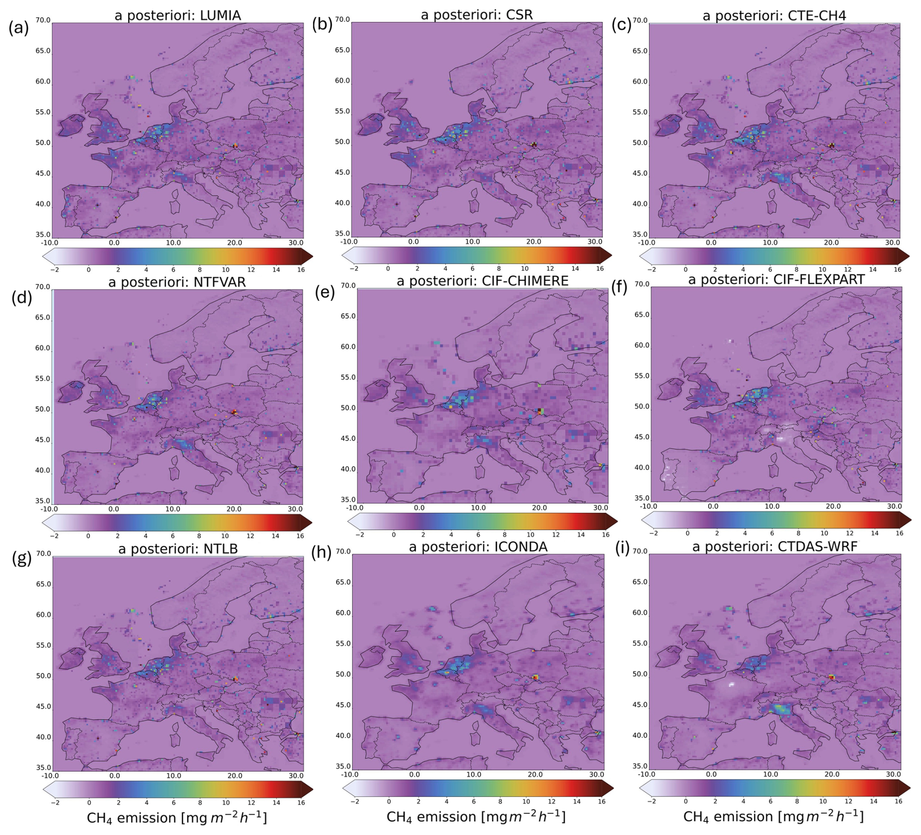
Figure C1 CH₄ emission fluxes, in mg m⁻² h⁻¹, over Europe, averaged for the common years 2008, 2013 and 2018, and the BASE simulation. The different panels show the a posteriori fluxes for the different inverse models: (a) LUMIA, (b) CSR, (c) CTE-CH₄, (d) NTFVAR, (e) CIF-CHIMERE, (f) CIF-FLEXPART, (g) NTLB, (h) ICONDA and (i) CTDAS-WRF.

Appendix D

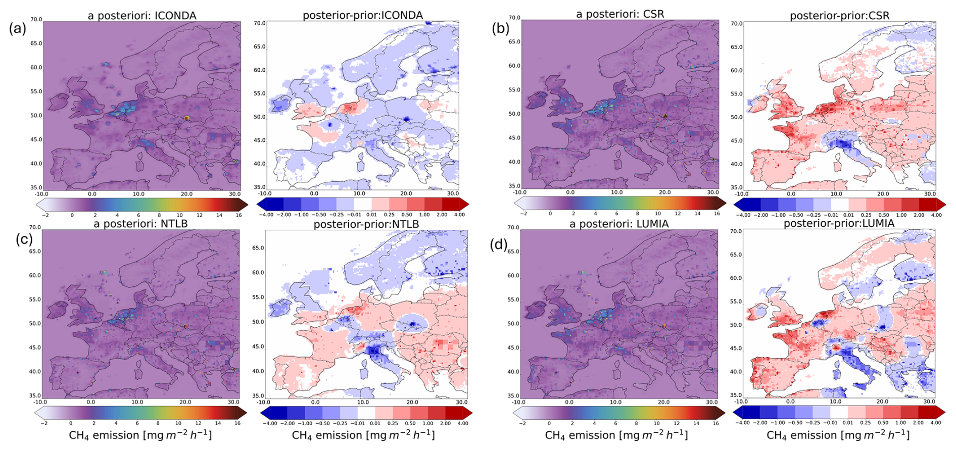
Figure D1 CH₄ emission fluxes, in mg m⁻² h⁻¹, over Europe, averaged for the common years 2008, 2013 and 2018, and the TEST simulation. The different panels show the a posteriori fluxes and the differences between a posteriori and a priori for the different inverse models: (a) ICONDA, (b) CSR, (c) NTLB, and (d) LUMIA.

Appendix E

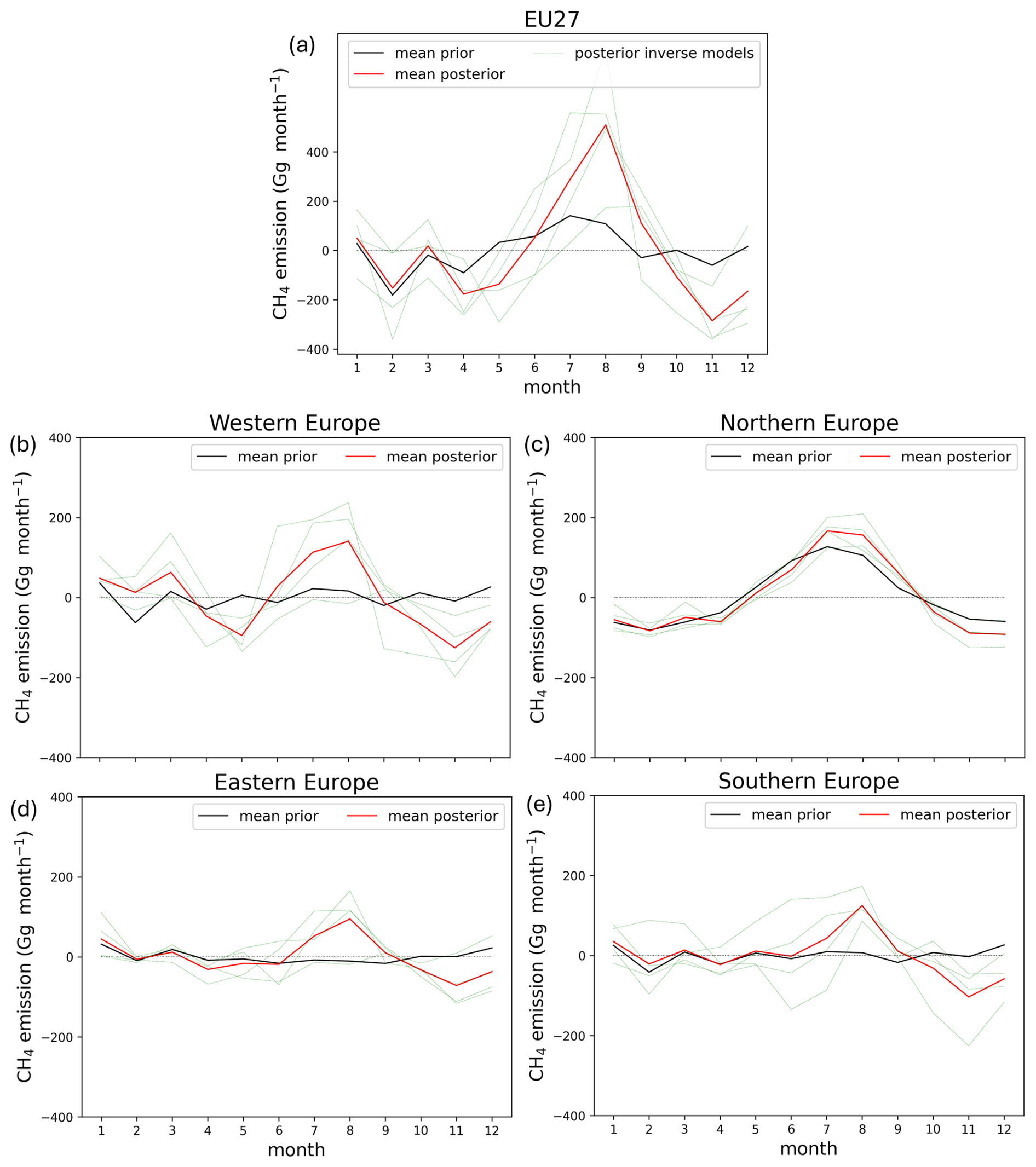
Figure E1 The same as Fig. 6, results are shown for the TEST simulation. Note that less inverse models provided results for the TEST run.