the Creative Commons Attribution 4.0 License.
the Creative Commons Attribution 4.0 License.
 | 19 Feb 2026
Optical complexity of North Sea, Baltic Sea, and adjacent coastal and inland waters derived from Sentinel-3 OLCI satellite data
Martin Hieronymi
Daniel Behr
Rüdiger Röttgers
Despite advances in remote sensing, consistent monitoring of water quality across freshwater-marine systems remains challenging due to methodological fragmentation. Here, we provide an overview of an exemplary dataset on water quality characteristics in inland waters, coasts, and the open sea estimated from optical satellite data (https://doi.org/10.26050/WDCC/AquaINFRA_Sentinel3_v2, Hieronymi et al., 2025). Specifically, this is Sentinel-3 OLCI (Ocean and Land Colour Instrument) data for the entire North Sea and Baltic Sea region for the period June to September 2023. The dataset includes daily aggregated observational data with a spatial resolution of approximately 300 m of reflectance at the top-of-atmosphere and for cloud-free water areas remote-sensing reflectance, inherent optical properties of the water, and an estimation of the concentrations of water constituents, e.g. related to the aquatic carbon content. These are the results of the novel A4O atmospheric correction and the ONNS water algorithm. The dataset serves as a prototype for understanding the processing chain and interdependencies, but also for developing a high degree of connectivity for answering various scientific questions; we do not perform an actual validation of the 73 individual parameters in the dataset. The challenges of a validation covering all water types are illustrated using one parameter, the particulate organic carbon concentration in water. The aim of this work is to show how fragmentation in water quality monitoring along the aquatic continuum from lakes, rivers to the sea can be overcome by applying an optical water type-specific and neural network-based processing scheme for Copernicus satellite data. Emphasis of this work is on analysing the optical complexity of remote-sensing reflectance in the North Sea, Baltic Sea, coastal, and inland waters. Results of a new optical water type classification show that almost all (99.7 %) remote-sensing reflectance spectra delivered by A4O are classifiable and that, based on this data, the region exhibits the full range of optical diversity of natural water bodies. The dataset can serve as a blueprint for a holistic view of the aquatic environment and is a step towards an observation-based digital twin component of the complex system.
- Article
(8149 KB) - Full-text XML
- BibTeX
- EndNote


Satellite remote sensing enables a continuous and global observation of the Earth system and the interactions of its compartments. Optical remote sensing, which measures the radiance of reflected sunlight in the ultraviolet to visible to near-infrared spectrum, allows large-scale observation of water surfaces, enabling effective assessment of aquatic ecosystems across the freshwater-sea continuum. With an image swath width of 1270 km and a spatial resolution nadir of approximately 300 m, the Ocean and Land Colour Instruments (OLCI) on board two Sentinel-3 satellites are particularly well suited for global water observation. The Sentinel-3 constellation operates on a near-polar and sun-synchronous orbit with images taken close to local noon. At full resolution, not only large marine areas but also complex coastlines, broad rivers, and larger inland waters can be recorded. This enables the observation and evaluation of various issues, for example on drinking and bathing water quality, matter fluxes into the sea, the effects of human activities on the aquatic environment, and warnings of possible harmful algae blooms. However, different terminologies and inconsistent measurement practices are often used in limnology and oceanography. For a holistic view of the aquatic environment, it is therefore necessary to provide comprehensible and easily transferable reference values from satellite data. Moreover, for user-friendly usability, the data should not only be Findable, Accessible, Interoperable, and Re-usable (FAIR), they should also be scientifically documented, contain a thorough metadata description, and enable easy data handling, e.g. through clear labelling and definition of limits and uncertainties. Ideally, the storage-intensive satellite images are also available in a simple visualisation so that their useability can be checked easily, as large land-sea surfaces are usually not visible due to clouds.
Earth observation of large areas with different types of waters also poses significant challenges for analysing satellite images. This is mainly due to the optical effect of the water constituents, which are parameterized by their inherent optical properties (IOPs). In addition to the pure water itself, phytoplankton, coloured dissolved organic matter (CDOM), and suspended non-algae particles (NAP) contribute to the colour appearance of the water body (e.g. Bi et al., 2023). Phytoplankton biomass is characterised by the total concentration of chlorophyll a pigment (Chl in mg m−3). But the various algae species have different pigment compositions and occur in a wide range of colours (e.g. Xi et al., 2015; Lomas et al., 2024). CDOM is often a degradation product of phytoplankton and organic compounds and is discharged from rivers into the sea in high concentrations but can also be brought into the sea by precipitation (e.g. Nelson and Siegel, 2013; Juhls et al., 2019; Kieber et al., 2006). The optical effect of CDOM is an absorption and darkening of the water. Sediments are kept in suspension by water movement in rivers and lakes, or in shallow waters by currents, tides, and waves. Suspended particles increase the backscattering of the light in water and therefore result in relatively bright satellite image pixels. In addition to the water components mentioned, air bubbles, pollutants, and inelastic scattering processes can have an influence on the reflectance, but this is neglected here.
From the perspective of the satellite, however, the total signal from the water body is small compared to the atmosphere. And here too, the atmospheric properties and cloud conditions over inland waters and the ocean can vary considerably, e.g. due to land-originated dust or soot aerosols or maritime aerosols (e.g. Hess et al., 1998). The correction of all atmospheric influences, masking of clouds and provision of remote-sensing reflectance (Rrs in sr−1) valid for all water types is therefore a crucial step.
There are several methods for atmospheric correction (AC) and many water algorithms that derive water constituents from Rrs (e.g. Müller et al., 2015; Brewin et al., 2015). The methods are usually optimized for different water bodies. However, no method offers robust performance across all water types and special atmospheric conditions, and the uncertainties and application limits are often insufficiently characterized; Hieronymi et al. (2023a), González Vilas et al. (2024), and others have documented this for various atmospheric correction methods for OLCI. The standard OLCI Level-2 (water full resolution) baseline atmospheric correction is applied for all water surfaces but often delivers insufficient data quality for the Baltic Sea, many coastal, and inland waters, which is indicated, for example, by “negative” reflectance. In the Copernicus Marine Service, different algorithms are used for the North Sea (as part of the North-East Atlantic) and the Baltic Sea (Brando et al., 2024), although this also includes inconsistent variables and designations; inland waters are not included here. Corresponding information for some lakes is provided in the Copernicus Land Service, but also with their own designations and completely different data accessibility. For coastal marine waters, there are additional products with higher spatial resolution from Sentinel-2 MSI observations, but also with pixel-based algorithm switching (Brando et al., 2024). It should be the aim to cover all water areas uniformly and with adequate accuracy of all products.
Fuzzy logic classification of optical water types (OWT) quantitatively characterizes aquatic systems through continuous membership functions, overcoming the limitations of discrete classification schemes (e.g. Moore et al., 2001). This approach is particularly valuable for capturing transitional waters (e.g., river plume or algal bloom fronts), as also highlighted in studies of coastal and inland systems (Spyrakos et al., 2018; Atwood et al., 2024), where optical properties vary non-linearly with constituent concentrations. However, its effectiveness depends on valid Rrs across the entire spectrum – a requirement often compromised when a single AC method optimized for specific water type is used. Hieronymi et al. (2023a) analysed Rrs from five AC with different OWT classification methods and found that the OWT algorithms have focused too much either on marine or limnological applications. This is expressed in the sometimes very low classifiability of Rrs and the class assignment of spectral shapes. The study also demonstrated the significant advantages of an integrated adaptation of atmospheric correction and OWT classification method, which also applies to the down-stream water algorithms. The findings from this study led to the development of a novel, robust, and comprehensive OWT classification system (Bi and Hieronymi, 2024).
In this paper, we document a dataset of merged Sentinel-3 OLCI Earth observations from the A4O-ONNS processing chain (Hieronymi et al., 2017), which includes the results of the new OWT classification. The individual processing steps have not yet been adapted to each other and fundamental further developments will be implemented in the future. However, this dataset serves to visualise the overall system and to further develop the underlying algorithms, flags, and biogeo-optical relationships. This enables a systemic harmonization and optimization of the workflow, a validation of all water products and a more targeted estimation of the overall system uncertainties. The presentation of data from the current version of the algorithm enables feedback from users and aims to increase the data interoperability and FAIR-ness level; nonetheless, publication of the code itself is only planned in the medium term. The aim is to show how fragmentation in water quality monitoring along the aquatic continuum from lakes, rivers to the sea can be overcome by applying an optical water type-specific and neural network-based processing scheme for Copernicus satellite data (fundamentally similar to the CERTO project; Atwood et al., 2024). Furthermore, in this work, some recommendations are realised to better characterize phytoplankton diversity and aquatic carbon fluxes in the future (e.g. Bracher et al., 2017; Brewin et al., 2023). The focus of this work is on the optical characterization of the waters of the North Sea–Baltic Sea region.
2.1 Geographical region
The spatial coverage of the Earth observation data extends from longitude −4.48 to 30.3° and latitude 48.98 to 65.9°, both in 0.004° steps (Fig. 1). This covers the entire Baltic Sea and North Sea with parts of the Norwegian Sea and English Channel, even parts of the Irish Sea are included. The southern extent is defined by the inclusion of the entire Elbe River catchment. The spatial resolution of OLCI of approx. 300 m per pixel was tried to achieve for the overarching grid, resulting in an image size of 8695×4231 pixels in the coordinate reference system WGS 84 (EPSG:4326). Accordingly, smaller bodies of inland water and narrow rivers are not covered.
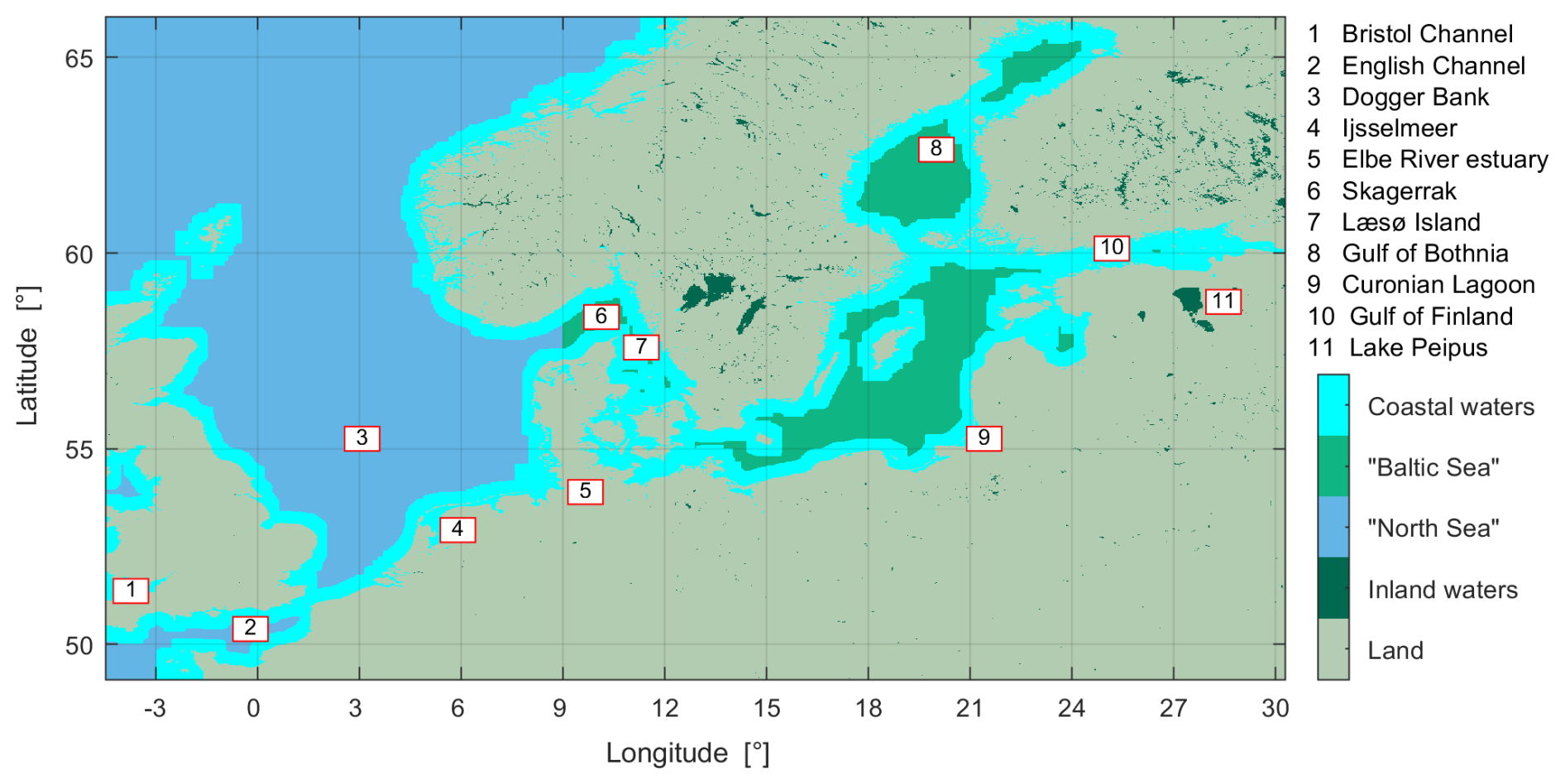
Figure 1Region of interest with definition of subdomains for optical water type analysis. Some areas mentioned in the text have been marked.
Four regional subdomains are defined for an initial categorisation of the optical diversity of the water bodies: North Sea, Baltic Sea, inland waters, and coastal waters; this is inspired by the domains in the Copernicus services (Brando et al., 2024). In terms of optical properties, the geographical subdomain “North Sea” is representative for the Copernicus Marine Service product for the Atlantic-European North-West Shelf which includes part of the Skagerrak in the east. In the Copernicus Marine Service, the Baltic Sea region is defined as an independent product, which also includes parts of the Skagerrak in the west at approx. 9° E. Correspondingly, a line at 9° E between Denmark and Norway is used to geographically separate the North Sea from the Baltic Sea. The inland waters subdomain contains all water areas on land that are larger than the pixel resolution of approx. 300 m, i.e. mainly lakes but also some broad rivers such as the Elbe estuary. The Copernicus Land Monitoring Service offers Sentinel-3 OLCI-based lake water quality products and additionally 100 m data from Sentinel-2 MSI (CLMS S2, 2024; CLMS S3, 2024). In the optical characterisation of waters, the term “coastal waters” is often used; to define a subdomain for this, the 12 nautical mile zone of territorial coastal areas is used. In order to include brackish water areas of lagoons (e.g. the Curonian Lagoon), coastal lakes (e.g. the Ijsselmeer), and rivers influenced by the tide (e.g. the Lower Elbe), the coastal domain is defined as plus-minus 75 pixels along the coastal baseline (i.e. approx. ±22.5 km). The seaside zone roughly corresponds to the area of the high-resolution ocean colour product from the Copernicus Marine Service with 100 m resolution from Sentinel-2 MSI (CMEMS BAL, 2025; CMEMS NWS, 2025). The coastal waters therefore include parts of the other three domains. The images cover 36.8 million pixels in total, thereof are 61 % the fraction of land, 27 % North Sea, 11 % Baltic Sea, and 1 % inland waters. Coastal (or territorial) waters cover 13 %.
2.2 Original Copernicus data
The freely available Sentinel-3A and 3B OLCI Level-1 data was obtained from the Copernicus Data Space Ecosystem (https://dataspace.copernicus.eu, last access: 12 February 2026). All scenes with a contribution to the region of interest and within the four-month period 1 June to 30 September 2023 were downloaded and processed. Among other things, the period covers a dedicated validation campaign in the Baltic Sea, where all water parameters from the satellite dataset were determined in situ (Hieronymi et al., 2023b). Due to the polar orbit of the satellites, there are more frequent observation opportunities in the north and increasing gaps in the southern section (Fig. 2). The contributing images are taken around local noon, for this region within a time window of about three hours. It can therefore be said that the one-day (1 d) aggregated data is representative for local noon.
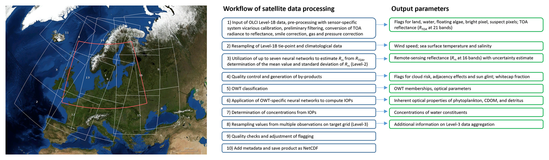
Figure 2Left: utilisation of all observational data within the region of interest (red frame) from individual OLCI scenes (white frames) from Sentinel-3A and 3B, which have shifted sun-synchronous orbits. Right: sequence of steps in the end-to-end processor with output parameters.
2.3 Processing chain
First, a summary of the evolution of the end-to-end satellite data processing scheme. The proposed algorithm is basically a further development of the Case-2 water algorithm by Doerffer and Schiller (2007), which was initially developed for ENVISAT MERIS and is currently being used for Sentinel-3 OLCI in the ground segment for coastal waters; this algorithm is also known as C2RCC (Brockmann et al., 2016; Müller et al., 2026). Parallel to the further evolution of C2RCC, an independent algorithm was branched off, the OLCI Neural Network Swarm (ONNS) algorithm by Hieronymi et al. (2017). This aims to generate reliable water quality parameters seamlessly for all natural waters and also to provide additional products, e.g. on carbon concentrations in water. The water algorithm ONNS uses its own OWT classification with 13 defined classes and specific neural network algorithms for each class. For some time, the ONNS water algorithm (with atmospheric correction from C2RCC) was used in the Copernicus Marine Service to estimate the chlorophyll concentration in the Baltic Sea (Le Traon et al., 2021). However, the classifiability of reflectance from different atmospheric corrections (incl. C2RCC) was often insufficient (Hieronymi et al., 2023a). For this reason, an independent new AC was developed by Hieronymi and colleagues, which was optimized for the performance spectrum of ONNS and called Atmospheric Correction for Optical Water Types (A4O). This AC method uses neural networks to approximate fully normalised remote-sensing reflectance (nadir sun and viewing zenith angles) at 16 bands from top-of-atmosphere reflectance at 21 OLCI bands. Wind influences are corrected to ensure standard assumptions for water algorithms; the wind speed is fixed at 5 m s−1, and the effects of whitecaps and air bubbles in the water are removed. These represent harmonised angles and environmental conditions designed to ensure global comparability and maximise the exploitation of satellite data, including under sun glint conditions. The underlying principles of this AC method A4O are very similar to those of C2RCC (Müller et al., 2026); however, it has not yet been comprehensively validated or published. Nevertheless, Hieronymi et al. (2023a) have shown validation results and according to them, A4O has the following particularly good performance compared to other accepted AC methods for OLCI: (1) a high classifiability of the generated Rrs in different OWT frameworks, i.e. basically plausible spectra in the entire spectral range (without Rrs<0), (2) general provision of spectra in all defined classes, (3) a high spatial homogeneity of the pixel-by-pixel image analysis and thus a particularly high number of achievable matchups. However, the comparison with in situ measurement data shows a need for further improvement; the reflectance spectra are often underestimated in magnitude (a normalization issue) – this is work-in-progress. Thus, the processing chain will be further optimized in terms of data quality, processing speed, data volume, and products including flags.
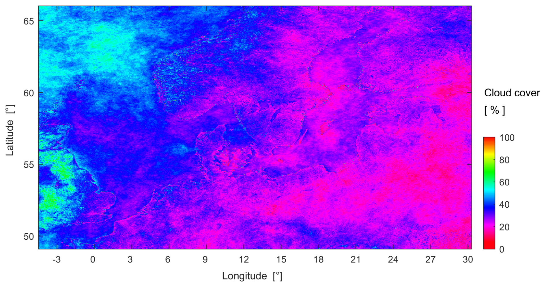
Figure 3Percentage cloud cover of the region over the entire period June–September 2023 (122 d) and thus indirectly clear-sky probability, which indicates pixel-based observation frequency. The coastlines can be subject to cloud misdetection. Contains modified Copernicus Sentinel-3 OLCI data [2023].
The workflow of the presented end-to-end processing chain A4O-ONNS v0.25 for daily aggregated observations is illustrated in Fig. 2. It consists of pre-processing (incl. smile correction and addition of climatological data), atmospheric correction, classification of optical water types, use of OWT-specific water algorithms, determination of water constituents based on IOPs, merging of daily averages, and storage with metadata. For daily observation, up to 17 individual OLCI Level-1 scenes of the same day with a volume of around 8 GB are processed, in the intermediate Level-2 step approx. 38 GB are produced, and the resulting merged Level-3 NetCDF files have a size of around 3 GB. So far, potential effects of tidal dynamics, particularly relevant in regions such as the Bristol Channel or the Elbe River estuary, have not been accounted for in the merging, which may influence the products (Sent et al., 2025). All cloud-free contributions are averaged within the superordinate grid. Due to the time offset between Sentinel-3A and 3B overflights and cloud motion, slightly more water surfaces can be seen, especially in the northern part, but this is irrelevant for the cloud statistics (Fig. 3). It should be noted, nevertheless, that the water-related products near clouds are usually subject to greater retrieval uncertainties. The optical water type classification of Bi and Hieronymi (2024) is applied to Rrs after merging. The final product contains selected information from Level-1 top-of-atmosphere, from climatology, the atmospheric correction, OWT classification, water products, and flags. Attention was paid to a concise metadata description, easy handling, and meaningful flagging.
2.4 Optical water type classification scheme
Water bodies in the study region are optically classified using the holistic OWT framework of Bi and Hieronymi (2024), which is summarised in the following. Unlike traditional approaches that cluster normalized reflectance spectra directly, this knowledge-driven framework classifies waters based on three derived optical variables: the apparent visible wavelength (AVW), the Box–Cox transformed spectral area (ABC), and the normalized difference index (NDI). These three variables project the high-dimensional hyperspectral information into a concise three-dimensional optical space, effectively capturing variations in both spectral shape and magnitude (Fig. 4a).
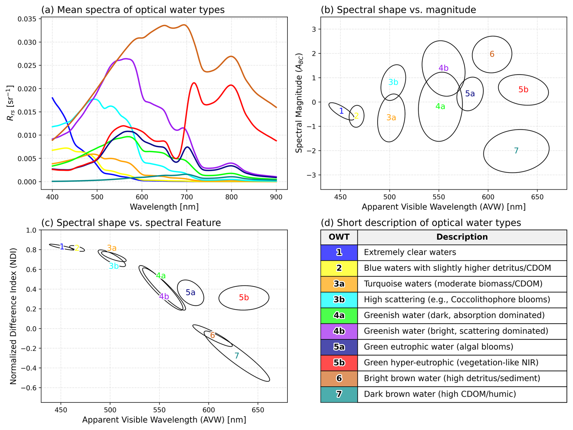
Figure 4Spectral characteristics and definitions of the optical water types from Bi and Hieronymi (2024). (a) Mean remote-sensing reflectance spectra for each type. (b, c) Distribution of OWT clusters across the three optical classification variables: apparent visible wavelength, spectral magnitude (ABC), and normalized difference index. (d) Descriptive summary of the ten water types.
Each variable represents a distinct optical characteristic (Fig. 4b and c). AVW acts as a spectral centroid, indicating the dominant hue of the water, ranging from short wavelengths in clear blue waters to longer wavelengths in turbid or productive waters. ABC, calculated from the integration of reflectance at red, green, and blue bands, quantifies the overall brightness or magnitude of the spectrum, which is primarily driven by particulate scattering. NDI captures specific spectral shape features around the green and red peaks, aiding in the discrimination of phytoplankton-dominated waters from those dominated by non-algal particles.
The framework defines ten distinct OWTs (Classes 1 to 7) representing the continuum from oligotrophic to hyper-eutrophic and extremely turbid waters (Fig. 4d). A key feature of this scheme, addressing the optical complexity of coastal transitions, is the subdivision of certain classes into “a” and “b” variants (e.g., 3a/3b). While “a” and “b” variants share similar spectral shapes (and thus similar AVW), they differ significantly in magnitude (ABC). “a” typically represents waters dominated by absorption or moderate scattering, appearing darker. In contrast, the “b” variants represent high-scattering conditions with significantly higher reflectance, such as those caused by coccolithophore blooms (OWT 3b and 4b) or suspended mineral sediments. OWT 5a and 5b specifically characterize productive waters with high phytoplankton biomass, where 5b represents hyper-eutrophic conditions with distinct vegetation-like spectral features in the near-infrared. OWT 6 and 7 represent the extremes of optically complex waters, dominated by high concentrations of total suspended matter (bright brown) and colored dissolved organic matter (dark/black), respectively.
The classification is implemented using a fuzzy logic approach based on the Mahalanobis distance in the three-dimensional variable space. For each satellite observation, the OWT algorithm calculates the membership probability for each type. The final class assignment is determined by the maximum membership, while the total membership serves as a quality indicator of how well the observed spectrum fits within the defined optical universe.
2.5 Additional data
The atmospheric correction A4O uses climatological data to better resolve influences of sea surface whitecaps and coastal conditions; these data are also provided. Climatological reanalysis data of sea surface temperature, SST, and salinity, SSS, have been adapted to A4O purposes with a global spatial resolution of 1/12° (approx. 8 km). Monthly mean temperature and yearly mean salinity were derived from the Copernicus Marine Service global ocean physics reanalysis (Lellouche et al., 2018) related to the period 1993 to 2016. Since this product contains no data for inland waters and lakes, monthly mean SST of larger lakes were derived from ERA5 data of the European Centre for Medium-Range Weather Forecasts (ECMWF, https://cds.climate.copernicus.eu/, last access: 12 February 2026; averaged over the years 1979 to 2020 and re-gridded from 30 km resolution). Missing values for any other inland waters were filled with the mean value of all grid cells on the same latitude of each month. Grid cells without a valid salinity value represent land or freshwater and were therefore assigned to a value of zero. Major saline lakes like Dead Sea or Great Salt Lake have been included manually. In practice, this gives a temperature between 0 and 36 °C and salinity values of 0 to 40 PSU. A Laplace filter is applied to the re-gridded SST and SSS during the satellite image processing to smooth grid boundaries. When using A4O, the data is projected onto the coordinates of the Level-1 OLCI scenes; in Level-3 processing, all data is projected onto the same global grid.
3.1 Overview of available parameters
An overview of all parameters contained in the data for each day is listed in the following, the corresponding units are in brackets, where 1 stands for unitless. Some parameters refer to the entire region of interest over land and water, such as top-of-atmosphere reflectance and wind speed. Products from climatologies and their derivatives, such as whitecap fraction, refer only to water areas resolved in the 300 m grid, i.e. for lakes, broad rivers, lagoons, and seas. Water quality characteristics are only provided for visible, cloud-free water areas. NaN (not a number) is used as fill values for corresponding data gaps.
Parameters from the original OLCI Level-1 data:
-
L1_land: Level-1 land mask (thus implicitly water areas) [1]
-
L1_Wind_speed: omnidirectional wind speed from Level-1 [m s−1].
Parameters from the atmospheric correction A4O:
-
A4O_R_toa_400–1020: reflectance at the top-of-atmosphere at 21 OLCI bands [1]
-
A4O_Rrs_n_400–1020: normalized remote-sensing reflectance at 16 OLCI bands [sr−1]
-
A4O_SST: monthly average of the sea surface temperature from climatology [°C]
-
A4O_SSS: annual average of the sea surface salinity from climatology [] or [PSU]
-
A4O_A_wc: percentage whitecap fraction of water areas based on wind speed and sea surface temperature [1] or [%].
Parameters associated with the optical water type classification (Bi and Hieronymi, 2024):
-
OWT_AVW: apparent visible wavelength based on A4O_Rrs_n between 400 and 800 nm [nm]
-
OWT_Area: trapezoidal area at red, green, and blue (RGB) bands based on A4O_Rrs_n [1]
-
OWT_NDI: normalized difference index at green and red based on A4O_Rrs_n [1]
-
OWT_index: optical water type index or class based on A4O_Rrs_n [1]
-
OWT_U_tot: total membership values in the OWT framework [1].
Parameters from the ONNS water algorithm (Hieronymi et al., 2017):
-
ONNS_a_g_440: gelbstoff (CDOM) absorption coefficient at 440 nm (from IOP nets) [m−1]
-
ONNS_a_p_440: absorption coefficient of phytoplankton particles at 440 nm [m−1]
-
ONNS_a_m_440: absorption coefficient of minerals at 440 nm [m−1]
-
ONNS_a_tot_440: total absorption coefficient at 440 nm of CDOM, phytoplankton, minerals, and water [m−1]
-
ONNS_b_p_440: scattering coefficient of phytoplankton particles at 440 nm [m−1]
-
ONNS_b_m_440: scattering coefficient of minerals at 440 nm [m−1]
-
ONNS_b_tot_440: total scattering coefficient at 440 nm of phytoplankton, minerals, and water [m−1]
-
ONNS_a_dg_412: absorption coefficient of detritus plus CDOM at 412 nm [m−1]
-
ONNS_b_bp_510: total back-scattering coefficient of all particles at 510 nm [m−1]
-
ONNS_FU: Forel–Ule colour index [1]
-
ONNS_K_d_490: diffuse attenuation coefficient of downwelling irradiance at 490 nm [m−1]
-
ONNS_K_u_490: diffuse attenuation coefficient of upwelling irradiance at 490 nm [m−1].
Parameters for concentrations of water constituents based on ONNS-derived inherent optical properties:
-
IOP_Chl: chlorophyll concentration estimated from total particulate absorption coefficient at 440 nm [mg m−3]
-
IOP_TSM: total suspended matter concentration estimated from total particulate scattering coefficient at 440 nm [g m−3]
-
IOP_POC: total particulate organic carbon (POC) concentration based on inherent optical properties of phytoplankton and non-algae particles [g m−3]
-
IOP_DOC: concentration of dissolved organic carbon (DOC) related to CDOM absorption at 440 nm (Juhls et al., 2019) [mg m−3].
Available flags from the atmospheric correction and water algorithm
-
A4O_flag_cloud: cloud mask from A4O [1]
-
A4O_flag_cloud_risk: high risk of clouds, which can strongly influence the quality of the retrieval [1]
-
A4O_flag_adjacency: pixel near land or clouds with high risk of retrieval influence, e.g. through sub-pixel contamination of land, optically shallow water, aquatic plants or cloud edges [1]
-
A4O_flag_bright: Level-2 bright mask, that includes possible clouds and sea ice [1]
-
A4O_flag_suspect_pixel: Level-2 flag for possibly implausible AC output [1]
-
A4O_flag_floating: Level-2 flag for very high biomass and possibly floating algae [1]
-
A4O_flag_glint_risk: Level-2 flag for sun glint risk [1]
-
ONNS_limited_valid: estimated IOPs and concentration values are highly uncertain [1].
Additional information on Level-3 data aggregation
-
TOA_count: number of pixels from available satellite images at the top-of-atmosphere [1]
-
BOA_count: number of pixels from available cloud-free images after atmospheric correction at the bottom-of-atmosphere [1].
Background information on selected parameters is provided in the following.
3.2 Whitecap fraction
Information on the whitecap fraction is important, for example, for estimating the gas exchange at the air-sea interface, the heat flux, or the formation of marine aerosols. Despite the relatively small area of coverage, whitecaps are relevant for atmospheric correction due to their high reflectivity in contrast to dark water. The surface fraction covered with whitecaps, Awc, depends on wind speed and water temperature and is usually much smaller than 5 %. Whitecap fraction is parameterized based on global microwave satellite observations (with a frequency of 10 GHz; Albert et al., 2016). The estimated Awc is provided by the atmospheric correction A4O together with wind speed from OLCI Level-1 and sea surface temperature from monthly climatology, SST.
3.3 Concentrations of water constituents
The original ONNS algorithm by Hieronymi et al. (2017) applied an internal OWT classification and class-specific neural network (NN) algorithms to derive IOPs, light field parameters, and concentrations of water constituents directly. One reason for this was internal checks of system uncertainties. For a clearer, more flexible and purely physics-based derivation of the water constituents, the concentrations are now determined based on the NN-derived IOPs only. This is essentially the approach already promoted by Doerffer and Schiller (2007) and used in the OLCI Level-2 processing for Case-2 waters. To emphasise this, the concentration labels refer to IOPs and not to ONNS directly. Moreover, for concentrations of chlorophyll and total suspended matter, similar IOP-relationships were used as in Doerffer and Schiller (2007).
The chlorophyll concentration is linked to phytoplankton-pigment absorption, but due to previous modelling inadequacies in the optical component separation, it is estimated here from total particulate absorption at 440 nm (an interim approach that will be revised in future):
The concentration of total suspended matter is estimated from total particulate scattering coefficient at 440 nm with:
The analysis of optical measurement data (Röttgers et al., 2023) and concentration of particulate organic carbon, POC, shows clear dependencies on phytoplankton and mineral particles or detritus, especially for coastal waters. In addition to phytoplankton absorption at 440 nm, ONNS also derives the total backscattering coefficient of all particles at 510 nm. The concentration of particulate organic carbon is well represented by the following IOP-relationship:
Juhls et al. (2019) show that the concentration of dissolved organic carbon, DOC, can be estimated via the absorption coefficient of coloured dissolved organic matter at 440 nm (in the ONNS notation, subscript “g” stands for Gelbstoff as a synonym for CDOM). Their relationship is also applied here:
3.4 Parameters from the optical water type classification
The three optical variables and OWT classification results are included in the dataset. The spectral magnitude is described by OWT_Area, the area below the Rrs spectrum at three red, green, and blue (RGB) bands, also referred to as the zeroth spectral moment. The trapezoidal area is Box-Cox transformed to yield ABC, which is subsequently used for the OWT classification. The apparent visible wavelength, OWT_AVW, describes the weighted average of the wavelengths between 400 and 800 nm, also described as the first spectral moment. The normalised difference index between green and red, OWT_NDI, helps to distinguish between phytoplankton and detritus-dominated spectra. During the OWT analysis of the reflectance, weights are assigned to all defined classes, although typically only three to six classes contribute significantly. Thus, in addition to the index for the water class with maximum membership, the total membership of all contributing classes is also provided in the dataset (OWT_index and OWT_U_tot). The total membership serves as an indicator of the quality of the classifiability; a minimum requirement of 0.0001 is often used (e.g. Moore et al., 2001; Hieronymi et al., 2017, 2023a).
Figures 5–9 illustrate the available data for 1 d (8 July 2023) of the merged satellite image at the top-of-atmosphere, after atmospheric correction, as well as the three optical variables for the OWT classification. Figure 10 shows the resulting OWT classes with the highest membership for that day. In most cases, one class dominates in the OWT analysis and intuitive conclusions can be drawn about the reflectance spectrum (and corresponding water constituents or phytoplankton groups). At the boundaries between dominant water types, there is often a transition zone with approximately equal contributions from neighbouring types. For a full exploitation of the OWT method, the results of the specific water algorithms are mixed with corresponding weights in a fuzzy-logic approach.
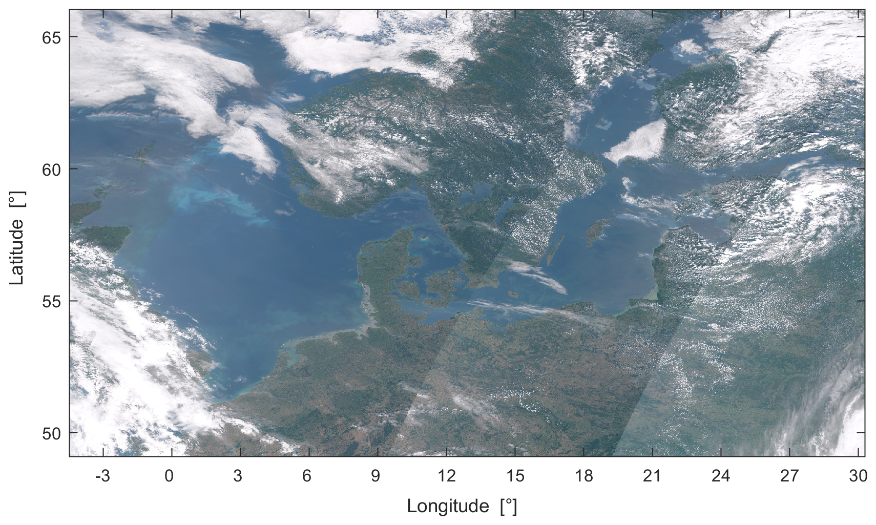
Figure 5RGB image created from reflectance top-of-atmosphere for 1 d (8 July 2023). It illustrates the starting point for the atmospheric correction including clouds, water-land areas, and observation angle effects at the original image margins. TOA information is also used for orientation over land and in case of cloud issues. Contains modified Copernicus Sentinel-3 OLCI data [2023].
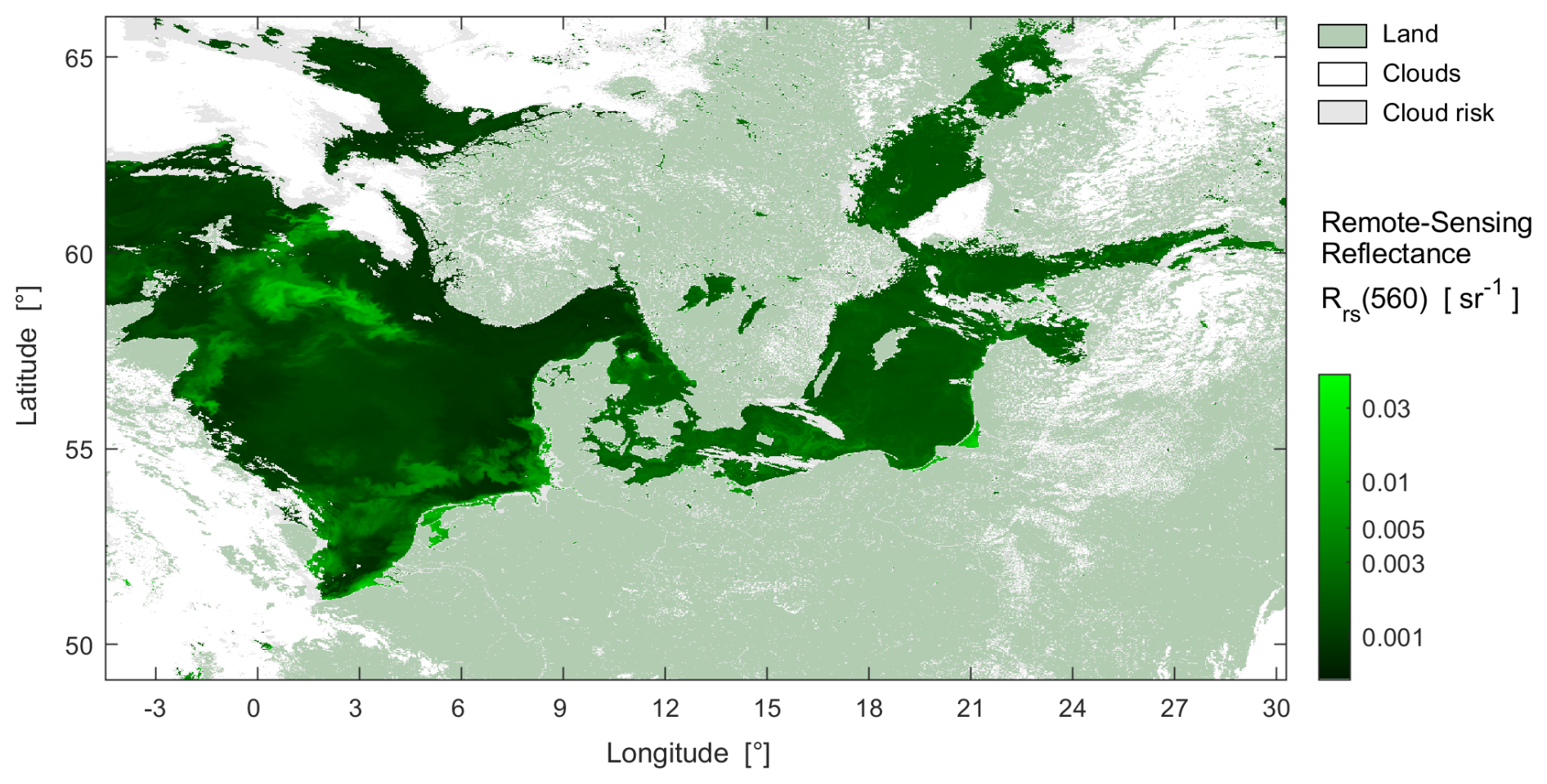
Figure 6Corresponding to Fig. 5, the result of the atmospheric correction: normalized remote-sensing reflectance at one wavelength (the green band at 560 nm) and labelling of land, clouds and cloud risk. Original image boundaries with increased “air mass” are no longer recognisable, only at cloud discontinuities. Contains modified Copernicus Sentinel-3 OLCI data [2023].
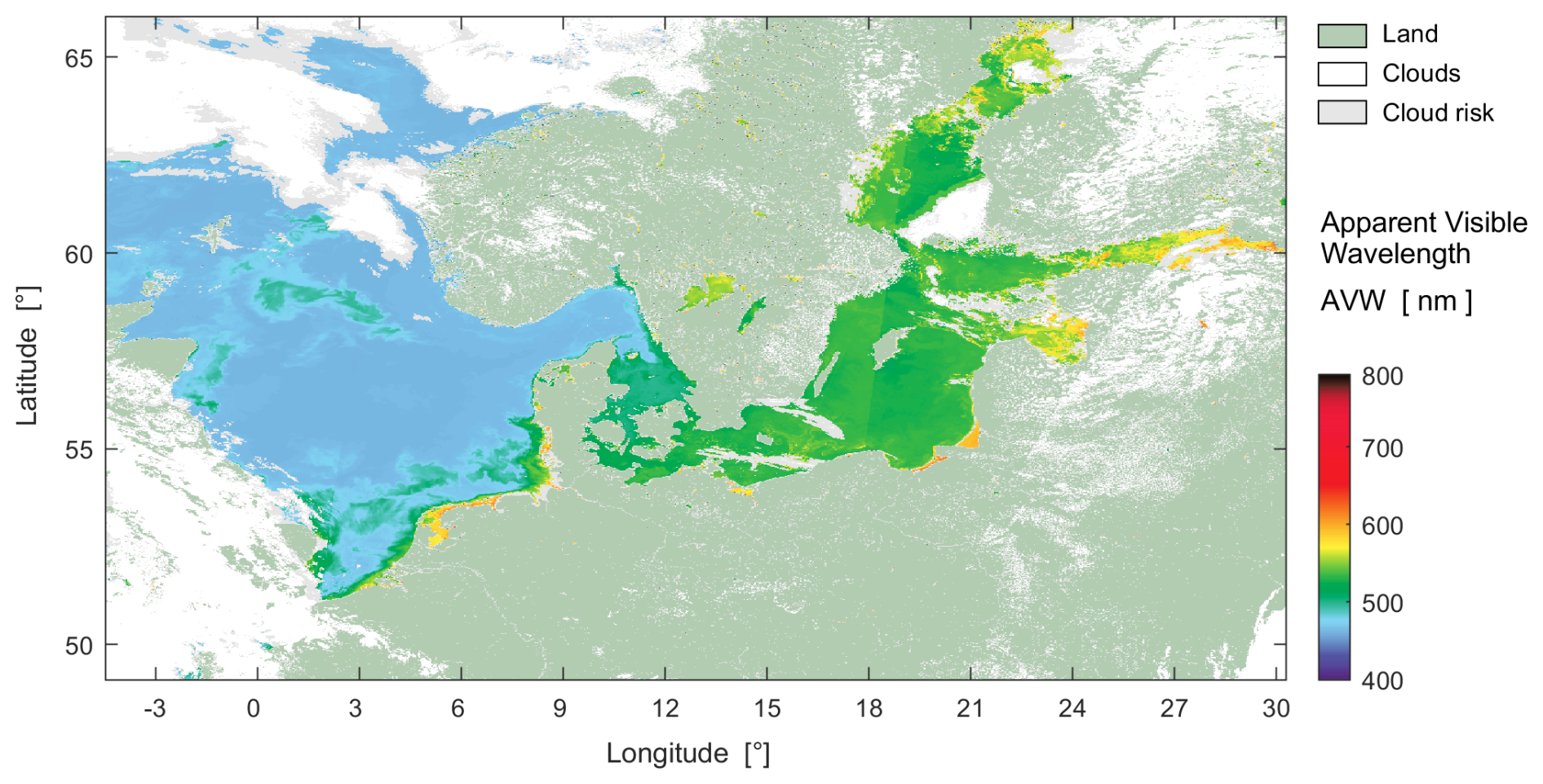
Figure 7Corresponding to Fig. 6, derived apparent visible wavelength with reference to the spectral range 400 to 800 nm for OWT classification. Contains modified Copernicus Sentinel-3 OLCI data [2023].
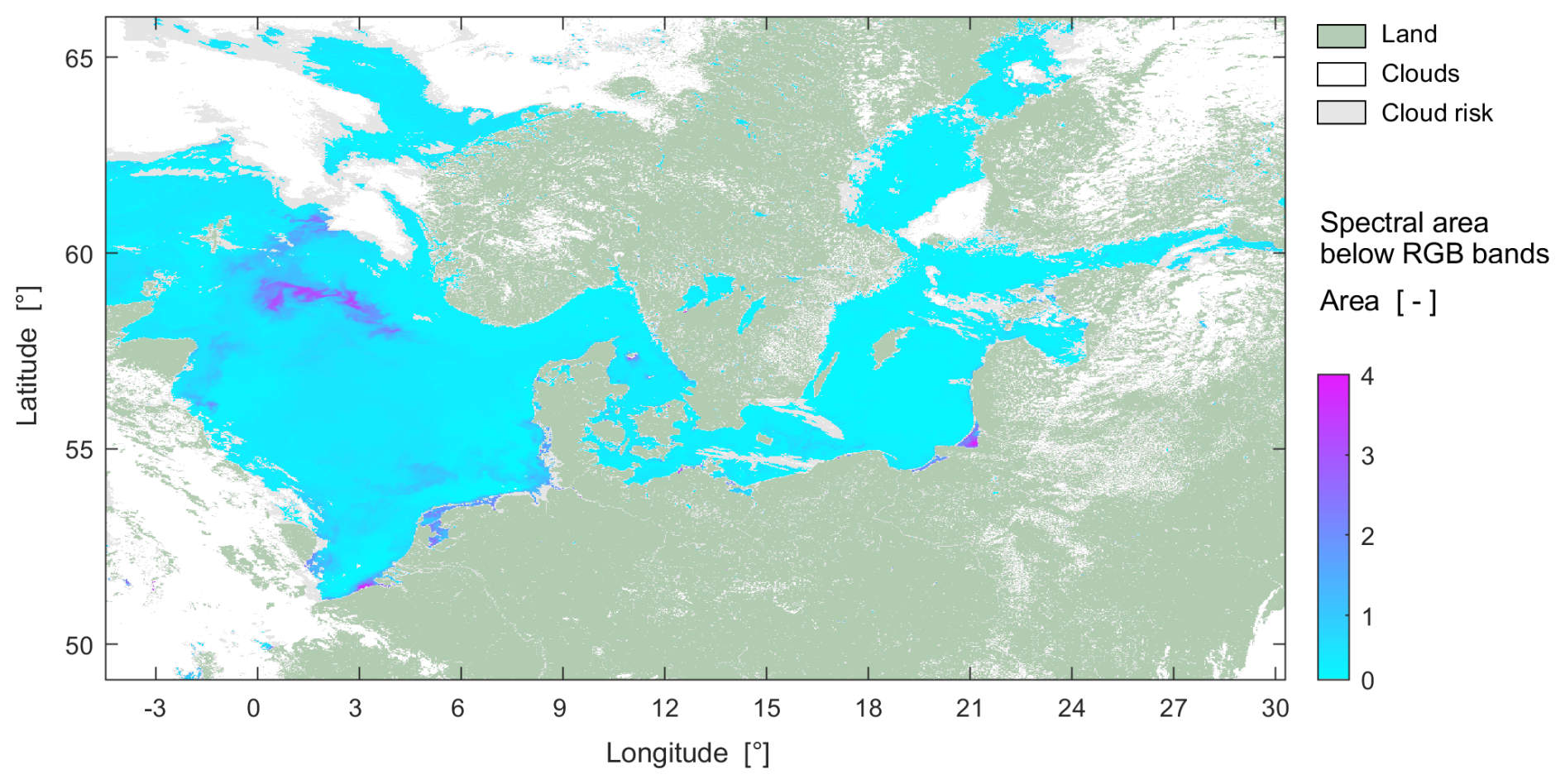
Figure 8Corresponding to Fig. 6, derived spectral area below Rrs at 443, 560, and 665 nm. This map shows the raw trapezoidal area, which is Box–Cox transformed into ABC for the actual OWT classification as presented in Fig. 4b. Contains modified Copernicus Sentinel-3 OLCI data [2023].
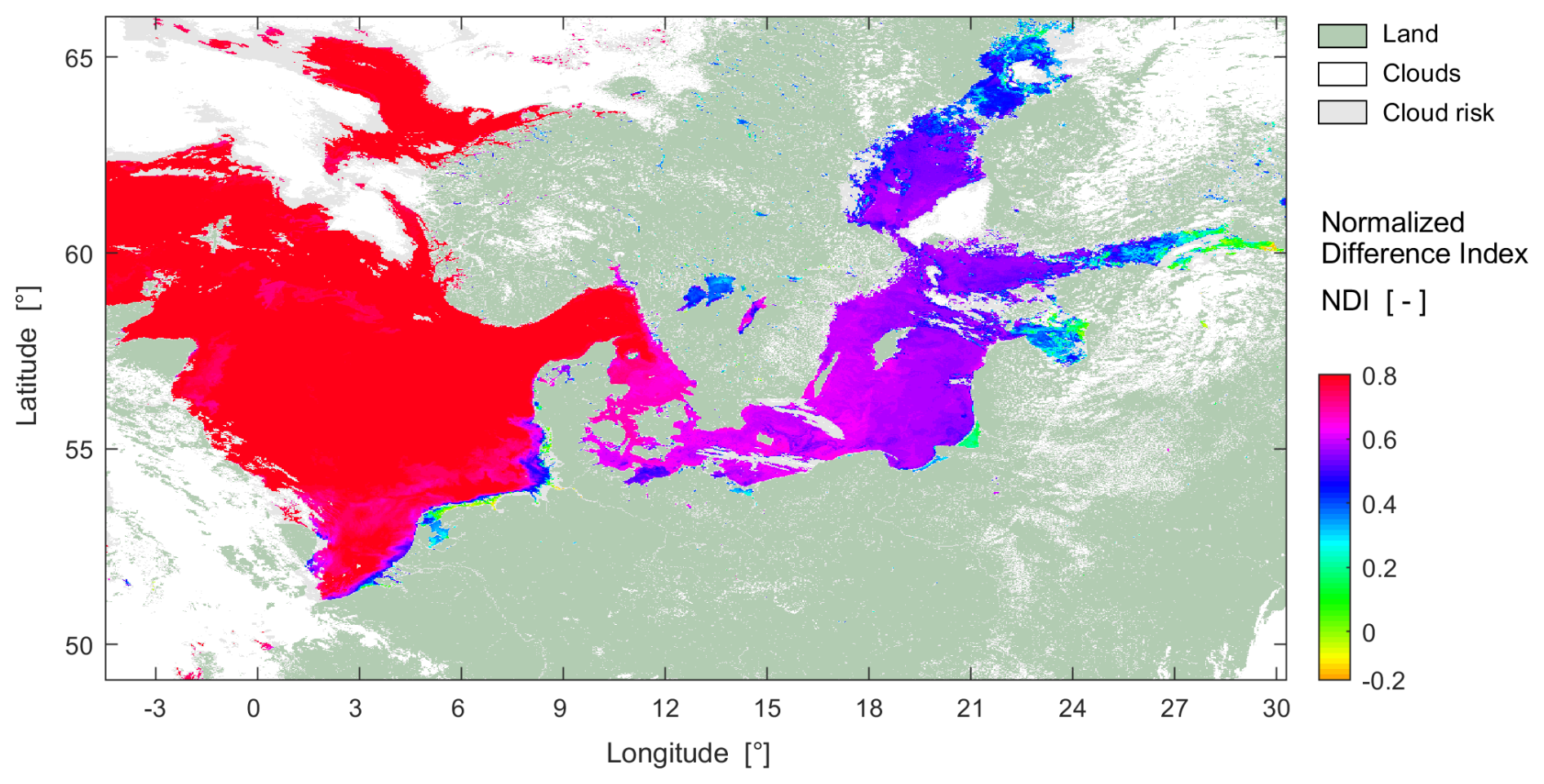
Figure 9Corresponding to Fig. 6, derived normalized difference index for OWT classification. Contains modified Copernicus Sentinel-3 OLCI data [2023].
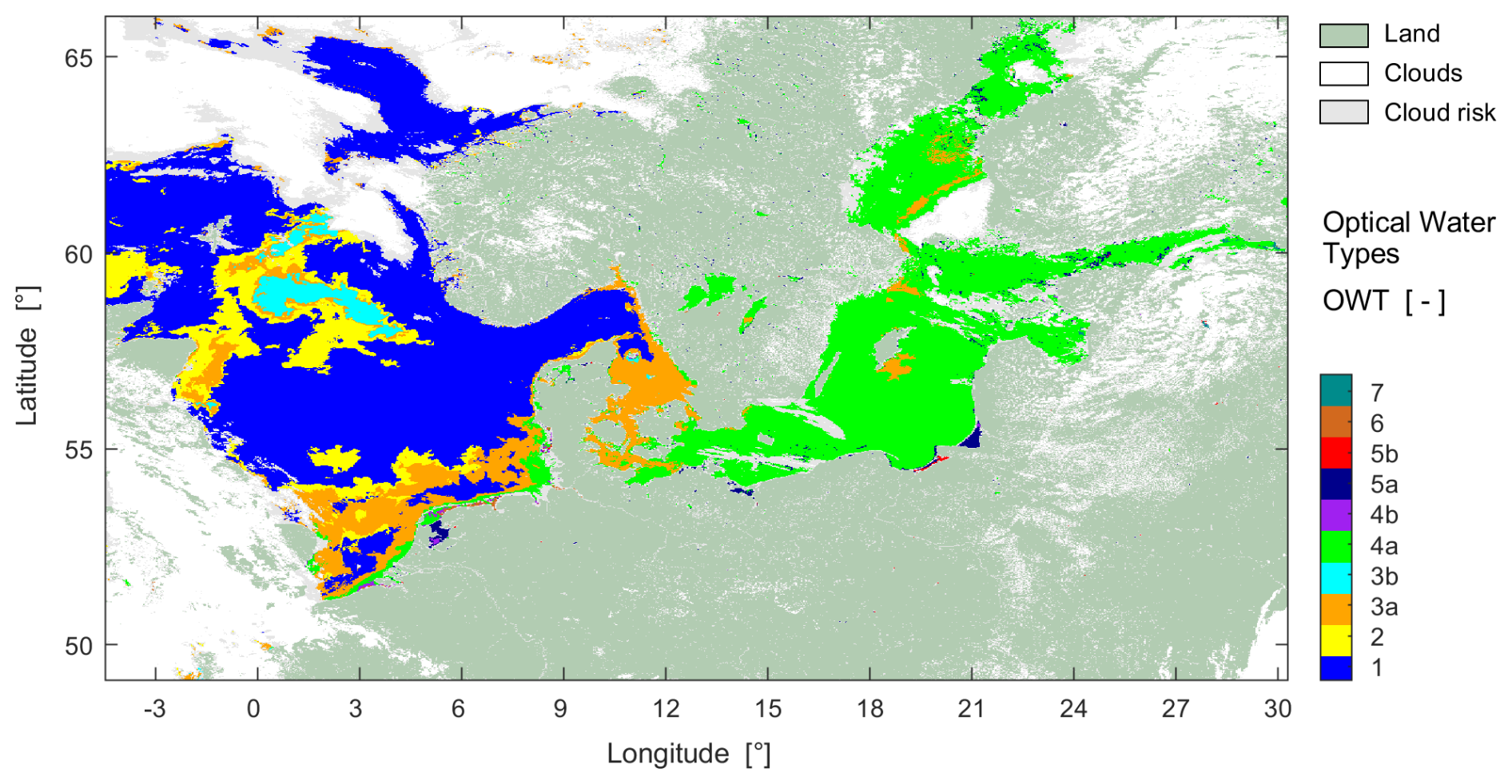
Figure 10Corresponding to Fig. 6, resulting water types with maximum membership. Seven spectral Rrs shapes are distinguished in the OWT framework; the subdivision into “a” and “b” shows differences in magnitude. Contains modified Copernicus Sentinel-3 OLCI data [2023].
This section demonstrates the application potential of the optical water type classification data through a representative analysis of summer 2023 patterns in the North Sea and Baltic Sea region, showcasing how the dataset can elucidate water mass dynamics and ecological transitions. Figure 11 shows a map of the water classes with maximum memberships that occur most frequently in the four-month period. This demonstrates a fundamental distinction between North Sea and Baltic Sea, which also justifies the regional split of the products in the Copernicus Marine Service (Brando et al., 2024). Coastal and inland waters vary more in colour and are often dominated by optical effects from high concentrations of sediments, CDOM, or phytoplankton. This wide range of concentrations may also exceed the validity range of applied satellite algorithms. Hieronymi et al. (2023a) compared five atmospheric correction methods for OLCI and showed that, especially in the transition from coastal to clearer North Sea waters, the resulting Rrs can be fundamentally different. Here, the comparative uncertainties in the shape and magnitude of Rrs are particularly high, but also difficult to quantify. Comparison with in situ data show a tendency for A4O to assess the water as clearer and bluer, i.e. to switch earlier than the other methods to maximum membership in OWT 1 during the transition to the open sea. Consequently, this means that absorption and scattering of water constituents are underestimated, and therefore the predicted concentrations are underestimated too. However, Hieronymi et al. (2023a) also documented some significant problems with the plausibility and classifiability of the results from the other atmospheric correction methods, e.g. to large-scale overcorrection with (incorrect) Rrs<0 or significant excess of Rrs especially in blue bands. This requires further studies and comparisons with in situ measurements.
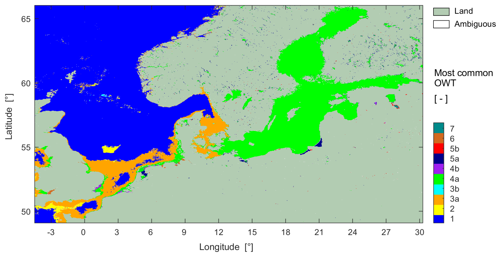
Figure 11Most common water types with maximum membership within June–September 2023. Contains modified Copernicus Sentinel-3 OLCI data [2023].
In general, however, the regional distributions show features that are reasonable from an oceanographic-limnological point of view. Figure 10 shows areas in the central North Sea with OWT 3b, a class that is intended to represent bright-turquoise blooms of coccolithophores, which contain high amounts of particulate inorganic carbon (calcite particles). Such bright pixels are sometimes flagged as clouds in other algorithms; in any case, such cases are critical regarding the assumptions for chlorophyll estimation, but OWT-specific assumptions can help here. But the coccolithophore bloom (OWT 3b) in Fig. 10 is only a temporary event with a phenologically changing colour appearance like shown for example in Cazzaniga et al. (2021); blue water (OWT 1) is the actual background in that region during summertime (Fig. 11). Another feature is visible in the North Sea area at the Dogger Bank with OWT 2, where the water can be less than 20 m deep, which on the one hand can lead to hydrodynamic resuspension of sediments through waves, and on the other hand it is possible that influences of the shallow bottom can be seen. This shows a fundamental problem of ocean colour, namely that optically shallow waters cannot yet be reliably flagged without water depth information, which can lead to misinterpretations of biomass and other parameters. The problem of shallow water and visible seafloor is particularly recognisable near the island Læsø in the Kattegat, where the OWT variability is very high – in fact, this should be flagged, because underlying assumptions (of optically deep conditions) for the water algorithms are invalid. But even apart from such artefacts, the map shows that all defined OWTs occur, and the region thus well represents the optical variability of natural water bodies. But again, it is possible that A4O estimates something too “blue spectra” in relatively clear shelf sea water – however, there are also significant contributions from OWTs 2 and 3a.
Also of interest is a map showing the number of different classes with maximum membership over the entire period (Fig. 12). Typical water algorithms and atmospheric corrections may be out-of-scope for different OWTs, which is not the case for A4O and ONNS. Areas with many different OWTs indicate high dynamics of sediments or algal blooms with possible eutrophication issues. Examples of water bodies with high optical variability with up to six different dominant classes are some Estonian lakes, including the large Lake Peipus. Ansper-Toomsalu et al. (2024) compared satellite products with in situ data from these waters, including the A4O-ONNS processing described here. Their results show a need for improvements but are not yet conclusive. Ideally, the comparisons should be made in the context of the prevailing OWT, which can help the further development of the algorithm and formulation of uncertainties. In principle, there can also be differences in the reflectance shape and the allocation of the OWT due to clouds, subvisible clouds, cloud shadows, but also due to subpixel contamination by coastal vegetation such as reeds, which is then interpreted as high biomass class. Nevertheless, there are also areas that are optically dominated by only one class over the entire period, such as the tide-influenced muddy and very bright Bristol Channel with dominating OWT 6. For ground-truthing and definition of system vicarious calibration (SVC) gains, low optical variability over time is more important than water clarity alone. While SVC is traditionally performed in clear waters, stable optically complex waters are essential for validating algorithms and ground-truthing across the full spectral range. OWT technology provides the opportunity to apply SVC on a per-water-type and per-product basis. Analysing the recurring patchiness of water classes can support the selection of representative sites for water quality monitoring and satellite validation (Lehmann et al., 2021).
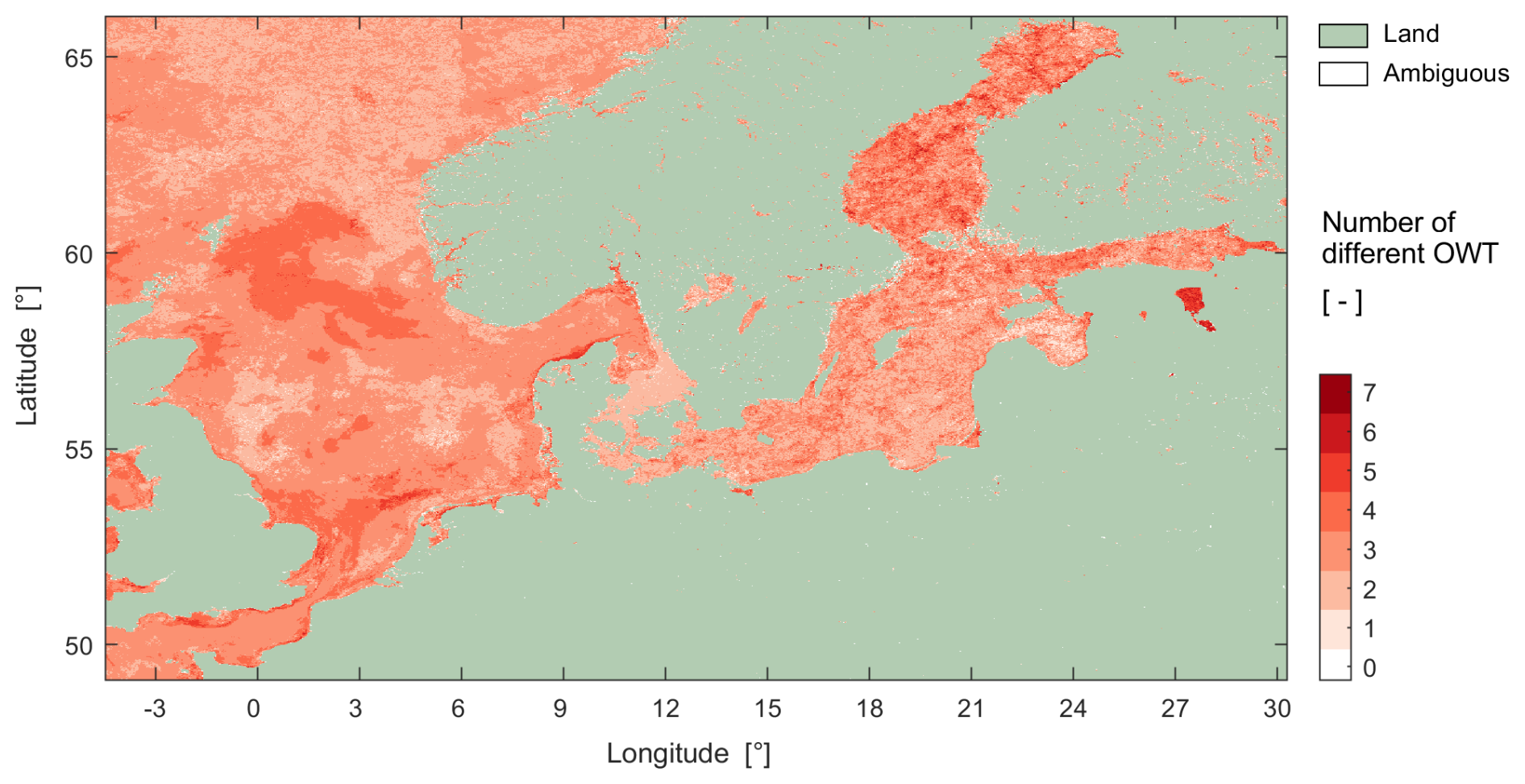
Figure 12Number of different water types with maximum membership within June–September 2023, i.e. the ecologically and hydrodynamically caused changes in water colour during the summer months. Contains modified Copernicus Sentinel-3 OLCI data [2023].
The occurrence of water classes and their classifiability for the entire region and period is shown in Fig. 13. This is a form of visualisation as already used in Hieronymi et al. (2023a) and Bi and Hieronymi (2024) (and their supplement), and in comparison with their results, Fig. 13 shows that Rrs from A4O can be well-classified with this OWT framework (99.68 % of the cases lead to a minimum total membership of 0.0001) and that all classes are filled. This is a significant benefit of A4O, but also of the OWT framework, and demonstrates the fitness for purpose of both methods for satellite monitoring of the land–sea aquatic continuum.
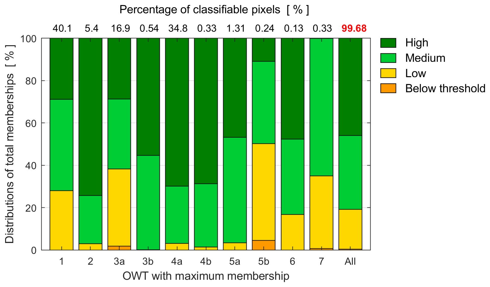
Figure 13Distribution of optical water types with maximum membership and category of their total memberships in high (>0.8), medium (0.3–0.8), low (0.0001–0.3), and below threshold (0–0.0001) for the entire region and period. The bar on the right gives the overall distribution. The figure corresponds to the illustrations in Hieronymi et al. (2023a) and Bi and Hieronymi (2024).
Using the regional subdivisions shown in Fig. 1, which are aligned with the domains in the Copernicus services, the optical properties of the water areas can be further specified. Table 1 shows the distribution of occurring water classes with maximum memberships and the overall level of classifiability in the subdomains. The very few non-classifiable cases, where the sum of the class memberships does not exceed the threshold value of 0.0001, are mostly associated with clouds, e.g. in 0.53 % of cases for the North Sea where the overall cloud cover is also higher (Fig. 3).
Table 1Percentage distribution of occurring water classes in regional subdomains and overall classification level.
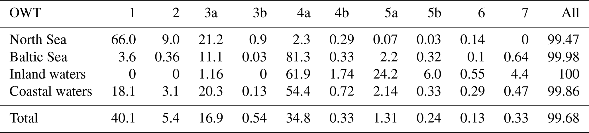
In the North Sea region (which here includes other parts of the European North-West Shelf Sea), the oceanic water types 1 to 3a dominate (with a total of 96.2 %). The bloom of coccolithophores visible in Fig. 10 is characterised by OWT 2, 3a, and 3b. The transitional waters to the southern coasts are more strongly influenced by CDOM input and sediment resuspension (OWT 4a and 4b). Thus, the spatial distribution of the classes also reflects the bathymetry of the North Sea.
The Baltic Sea is optically dominated by CDOM absorption effects and OWT 4a (81.3 %). The Skagerrak-Kattegat region is the transition to clear waters and marine salinity. As mentioned, there are some cases of optically shallow water with a visible sea floor for which OWT classes can serve as a mask, because the usual model assumptions for estimation of water constituents do not apply. OWT 5a and 5b also occur in the Baltic Sea. These classes represent green eutrophic to hypereutrophic waters with significantly higher phytoplankton biomass and bimodal reflectance shape. In the Baltic Sea, this is mostly associated with cyanobacteria blooms. The occurrence of these water classes can therefore be used directly as an indicator for cyanobacterial blooms. OWT 7 stands for dark brown waters with a very high CDOM concentration and low reflection in the entire visible range. This class of water is found in the Baltic Sea particularly near river outflows in the Gulf of Finland and the Gulf of Bothnia.
Inland waters are generally more characterised by CDOM absorption and its reflectance attenuation in the blue (e.g., Nelson and Siegel, 2013; Kutser et al., 2016; Spyrakos et al., 2018). Accordingly, oceanic water classes are not listed as predominant in this region. However, this could be the case in other regions of the world, e.g. in very clear oligotrophic lakes. Most inland waters fall into classes 4a, 5a, and 7, all of which have relatively high CDOM effects. Over 30 % of the water bodies also have high concentrations of algae (5a and 5b), therefore the OWTs are also characteristic for the trophic state of inland waters. OWT 6 stands for extremely scattering (NAP-dominated) turbid waters; they occur in some river estuaries like the tide-influenced Lower Elbe or Severn that flows into the Bristol Channel.
The category of coastal waters consists of parts of the other three subdomains and is optically the most diverse. Coastal waters range from oligotrophic ocean to hyper-eutrophic algal blooms and from bright-scattering to dark-absorbing. This means that the use of the term “coastal” for ocean colour algorithms is in fact somewhat misleading. The OLCI Level-2 coastal algorithm (or more precisely for optically complex waters), i.e. C2RCC, is optimised for moderately scattering or absorbing waters (Hieronymi et al., 2023a).
The dataset also contains several parameters that are useful for oceanographic-limnological, atmospheric, and biogeochemical process studies. Examples are outlined in the following.
5.1 Clouds
From global MODIS cloud observations, it is estimated that the fraction of clouds over worldwide land surfaces is about 55 %, with a distinctive seasonal cycle, whereas cloud cover over the oceans is around 72 %, with reduced seasonal variability (King et al., 2013). In our region of interest, summer tends to have fewer clouds than winter (e.g. Schrum et al., 2003), and our summer-dataset exhibits an overall lower cloud fraction compared to global climatology. The cloud cover averaged over the North Sea, Baltic Sea, and land areas (including inland waters) shows a relatively large daily variability and is significantly higher for the North Sea (41 %) than for the Baltic Sea and land areas in the region (both approx. 27 %) (Fig. 3). At the British Isles and north of them, cloud cover was on average often >60 %. The coastlines, and here in particular bright sandy beaches, are often misinterpreted as clouds (or cloud risk), which can be used for better flagging in the future. The cloud cover has an impact on the observable areas and possible matchups with satellites. Cloud cover also has an influence on the available solar radiation for photosynthesis of phytoplankton and is therefore crucial for estimating primary production. For example, neglecting photoacclimation of phytoplankton under clouds likely leads to a significant underestimation of growth rate and therefore of primary production (Begouen Demeaux et al., 2025). The available reflectances at top-of-atmosphere can be used to determine cloud shapes and brightness for cloud statistics, but also for better cloud-flagging and cloud-shadow detection in the future. Cloud motions and different correction methods also create problems when merging ocean colour data from different satellite missions for long time series (van Oostende et al., 2022).
5.2 Wind
The wind speed, i.e. the omnidirectional horizontal wind vector at 10 m altitude, is transferred from the OLCI Level-1 data and is available for all land-sea areas. Above water, wind influences the roughness of the water surface and wave development, the size of the direct sun glint area, the fraction of whitecaps at the surface due to wave breaking, the initial diffuseness of the underwater light field, but also the mixing of the upper water layer (e.g. Hieronymi and Macke, 2012; Hieronymi, 2016). This means that wind has an influence on the performance of the atmospheric correction, which is usually designed for moderate wind speeds, which is satisfied on average for the North Sea and Baltic Sea at 6.3 and 5.5 m s−1 respectively. However, there were also large-scale storm events during the observation period, e.g. at the beginning of August, which brought large amounts of precipitation to Scandinavia. Strong wind events also lead to surface-accumulated algae being mixed into the depths.
5.3 Carbon in the upper water column
Brewin et al. (2023) provide an overview of methods for obtaining ocean carbon from space, but also priorities, challenges, gaps, and opportunities for satellite estimates. Their review targets on both inorganic and organic pools of carbon in the ocean, in both dissolved and particulate form, as well as major fluxes of carbon between reservoirs (e.g. primary production) and at interfaces (e.g. air-sea and land-ocean). Extreme events, “blue carbon”, and carbon budgeting were also key topics discussed. Current algorithms include those that are: based on empirical band-ratio or band-differences in remote-sensing reflectance wavelengths; IOP-based; IOP and chlorophyll based; based on estimates of diffuse attenuation (Kd); and based on relationship between diffuse attenuation and IOPs. Our dataset contains most needed parameters required for the use of the various algorithms. Some information can be estimated from the local course of the sun and large-scale cloudiness, like the diurnal photosynthetically available radiation (PAR) that is essential for estimating primary production. Optical water types have the potential to support improved characterization of aquatic carbon. OWT 3b for example, which is especially defined for strongly backscattering coccolithophore blooms, serves as a direct hint for particulate inorganic carbon (PIC). The IOPs and reflectances provided allow quantification of PIC concentrations (e.g. Balch and Mitchel, 2023). The flag for floating algae is an indicator that recognizes scum at the surface or floating macroalgae such as Sargassum, which are part of the “blue carbon”. There are therefore extensive links in the dataset for estimating aquatic carbon.
We pursue the physics-based approach of determining the inherent optical properties of individual water constituents from aquatic reflectance. The optical effect of biogeochemical stocks can be reliably estimated using IOP-constituent relationships. The establishment of such relationships increases the traceability of individual processing steps. The concentration products in the dataset are based exclusively on the estimated IOPs and do not yet include any system vicarious calibration for the overall processing, which is an option for optimising validation results (e.g. O'Kane et al., 2024). In addition to the estimation of widely used concentrations of chlorophyll and total suspended matter, we also provide concentrations of dissolved and particulate organic carbon (DOC and POC). However, a matchup-based and OWT-specific validation of the products is still ongoing.
There is only very little measured and uncertainty-characterized validation data available for the same region and time. As an illustrative example, we discuss the challenges associated with satellite data validation using a single case study with POC. From a validation campaign with RV Alkor (AL597) in July 2023 in the Baltic Sea POC measurements are available with concentrations varying between 0.25 to 1 g m−3 (N=48). The related determination errors were generally low (1 %–5 %), but in few cases up to 20 % (Hieronymi et al., 2023b; Novak and Röttgers, 2026). Based on both measured and satellite-derived reflectance, the waters during all these measurements were assigned to just one optical water type, namely OWT 4a. Nevertheless, there are considerable small-scale spatial variations, often caused by the occurrence of large cyanobacteria colonies. Standard matchup criteria require a narrow time window and spatial homogeneity, but cloud cover also limits the amount of available comparison data. To estimate retrieval performance, we use all measurement points and corresponding satellite observations for the entire month of July 2023 (monthly average in Fig. 14). Figure 15 shows a comparison of POC values from satellite observations with median of values from 3×3 pixels using a homogeneity criterion and cloud-free conditions within 5×5 pixels. The error bars for satellite-derived POC represent the minima and maxima of the mean values for the month and indicate that the values can vary by an order of magnitude, which is often related to unrecognized cloud artefacts (typically resulting in higher POC concentrations). This shows that rigorous system-wide flagging needs to be improved. However, Pearson's correlation coefficient shows a strong positive relationship (r=0.76). The absolute root-mean-square error (RMSE) is 0.25, the mean absolute error (MAE) is 0.23, and the median absolute relative difference (MARD) (like in Smith et al., 2018) is 45 %. Linear regression yields a slope of 0.6 and an intercept close to zero; POC is therefore rather underestimated with considerable variability. However, we argue that explicit uncertainty characterization is also the dimension of high-quality Earth observation data. This rough comparison (for one water type) is similar to the other OC products in the dataset and shows that there is still substantial need for improvement of the end-to-end processor. However, it also shows the opportunities for OWT-specific adaptation of IOP-concentration relationships and application of system vicarious calibration.
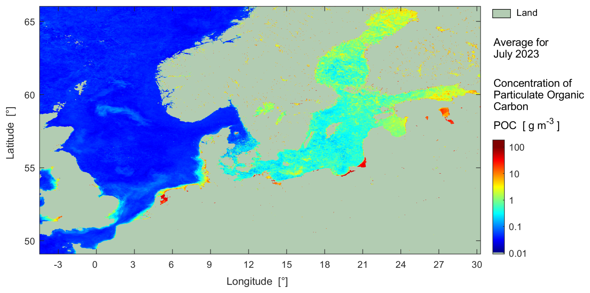
Figure 14July-monthly-averaged IOP-based estimate of the concentration of particulate organic carbon in the upper water column. Contains modified Copernicus Sentinel-3 OLCI data [2023].
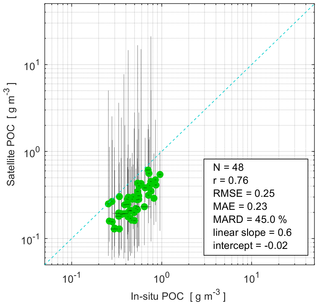
Figure 15Comparison of particulate organic carbon measured in situ from water in the Baltic Sea against satellite estimates from the same month (July 2023, like Fig. 14). The horizontal error bars of the in situ POC concentrations represent the standard errors from the determination. Vertical lines show the variation in median values in 3×3 pixels of the satellite images over the entire month. The 1:1 line is represented by a dashed line.
Our POC measurements in the North Sea region usually show values of 0.05 to 0.5 g m−3; in the turbid parts of the German Bight and in the Elbe estuary, POC values up to 15 g m−3 have been measured (Röttgers et al., 2023; Novak and Röttgers, 2026). These are the magnitudes of POC concentrations that are mirrored in the dataset and shown in the monthly average in Fig. 14. Existing POC algorithms are often optimised for lower concentration ranges of oceans, e.g. Stramski et al. (2008), but there are also others that target higher coastal concentrations such as Loisel et al. (2023). Ultimately, their performance also depends on accurate atmospheric correction. The aim of our efforts with A4O and OWT-specific IOP-concentration relationships is to cover the entire span of concentrations over several orders of magnitude.
The complete satellite image processing chain of atmospheric correction, OWT results, IOP algorithm, IOP-constituent relationships, and day-aggregated data is still work in progress and requires better harmonisation of the components. Individual parts, such as the atmospheric correction (A4O) and the water algorithm (ONNS), provide each an estimate of the uncertainties for the derived outputs – but these sub-results are not provided in the present dataset. These original uncertainty estimates are sometimes misleading because they do not take into account the other components, especially the coupling of atmospheric correction and water retrieval, but also not the higher-level flagging and actual comparisons with in situ measurements.
The spatial visualisation of the data gives indications of occasional imperfections, e.g. regarding flagging of clouds, nearby land, shallow water, sun glint, and tidal flats, but also viewing geometry effects from the atmospheric correction, which are sometimes mirrored in water products. Parameters such as CDOM absorption coefficient (and the corresponding directly derived DOC concentration) are particularly sensitive to smallest errors of the atmospheric correction due to the ambiguities of the system and the absolute signal dominance of Rayleigh light scattering in the atmosphere. Very high concentrations of CDOM are usually found in small inland waters and are discharged into the sea via rivers, which can lead to additional risks in monitoring due to relatively coarse spatial resolution and land-adjacency effects (e.g. El Kassar et al., 2023).
The provision of a masking recommendation or invalid-pixel expression for the end-to-end processing scheme is the subject of ongoing research. For example, results from areas with high sun glint are merged in the daily means; the results appear plausible, but they would be flagged in other AC methods (e.g. Hieronymi et al., 2023a). We primarily recommend enabling the “cloud risk” filter and paying attention to spatial inhomogeneities related to undetected clouds, and, if necessary, excluding such areas from comparative analyses and subsequent data processing as well.
The ambitions of the overall algorithm are very challenging, especially since a biogeo-optical system is to be described in an all-water type-comprehensive and open-connectable way, but all parameters basically vary over several orders of magnitude in their value ranges. Mission requirements for uncertainties are often defined in a simplified manner in the context of Case-1 and Case-2 waters, but requirements are not specified for all variables, e.g. IOPs (e.g. IOCCG, 2019). A more concrete OWT-specific guideline could help here; however, this also includes extreme waters that can exhibit very high uncertainties.
The underlying algorithm setup has not yet been sufficiently validated for each water type; some variables and preliminary elements were addressed in Hieronymi et al. (2023a) and Ansper-Toomsalu et al. (2024). On the one hand, there are many parameters that are useful for the spectral system description and serve as links for various empirical algorithms; on the other hand, some parameters are rarely measured and are not available for all defined water types. In fact, the current efforts of FAIR data preparation are aimed at finding suitable validation data and contextualising the satellite products. The user-oriented, traceable, and simple categorization of uncertainties is a focus of ongoing research.
An obvious and important goal is the appropriate validation of the parameters of the dataset and the processing chain in general, especially those related to water quality. Methodologically, five groups with specific requirements are distinguished here: remote-sensing reflectance (16 values), diffuse attenuation of irradiance (two), colour index (one), inherent optical properties (nine), and concentrations of water constituents (four). In addition, there are meteorological (wind, solar irradiation, and cloud cover) and limnological-oceanographic (water temperature and salinity) parameters in the dataset that have not been verified. We are convinced that it would be beneficial to carry out the validation in the context of optical water type classification; the approach by Bi and Hieronymi (2024), which distinguishes ten classes, is ideal for this. Alternatively, other OWT frameworks can serve as a basis (e.g. Moore et al., 2001, 2014; Vantrepotte et al., 2012; Mélin and Vantrepotte, 2015; Jackson et al., 2017; Spyrakos et al., 2018; Bi et al., 2021; Atwood et al., 2024). However, some of these frameworks differentiate a large number of optical classes (e.g., up to 17). While scientifically rigorous, such high granularity can be challenging for operational validation, where a more consolidated set of classes is advantageous to ensure sufficient matchup density for robust statistical assessment of each water type. Ideally, one can utilise matchups in which all parameters were measured simultaneously, e.g. as on the dedicated research cruise in the Baltic Sea in July 2023 (Hieronymi et al., 2023b) – but this also only covers one water class. We aim to utilise new data handling technologies, such as the AquaINFRA Data Discovery and Access System (https://aquainfra.eu/, last access: 12 February 2026), which allows researchers to seamlessly find and retrieve datasets from heterogeneous sources, e.g. from stationary or moving measurement platforms, from long time series or targeted experiments. Overall, further harmonization of standard names is required, for example according to CF conventions, in a manner that is scientifically appropriate for both oceanographic and limnological contexts. In perspective, this dataset and the underlying algorithms are an opportunity for the exploitation of remote sensing in order to answer limnological-oceanographic questions and expand monitoring capabilities. This could, for example, be a contribution to observation-based carbon budgeting (e.g. Friedlingstein et al., 2023; Brewin et al., 2023), whereby coastal DOC and POC are already provided and there are many links for estimating PIC concentration and primary production in water. As has been shown, the optical water types are particularly useful as indicators for phytoplankton groups, and there is potential to better assess the phytoplankton function in the ecosystem, contextualising long-term observations, or to warn of harmful algal bloom (e.g. Bracher et al., 2017; Kordubel et al., 2024; Devreker et al., 2025).
8.1 Data availability
The dataset consists of 122 d-aggregated single NetCDF files totalling 365.16 GB. It can be freely obtained from the World Data Center for Climate at https://doi.org/10.26050/WDCC/AquaINFRA_Sentinel3_v2 (Hieronymi et al., 2025). Identical Sentinel-3 OLCI-based datasets with the same parameters have been produced for testing purposes for other regions of the world and will be made available soon at the same database: (1) the Mackenzie River region with the Beaufort Sea and Arctic Ocean, (2) the Black Sea with the Sea of Marmara and part of the Aegean Sea, and (3) the central North Atlantic.
8.2 Data visualisation
The NetCDF data can be opened and visualised in the Sentinel Application Toolbox SNAP or in QGIS, for example. In addition, there is a visualisation of the content using cloud-optimised GeoTIFFs, which was provided by the EU AquaINFRA project partner Finnish Geospatial Research Institute at the National Land Survey of Finland. This can be used to quickly check the actual availability of cloud-free water quality parameters of the Sentinel-3 OLCI ONNS dataset in two projected coordinate systems, namely
-
Pseudo Mercator: https://vm4072.kaj.pouta.csc.fi/ddas/oapic/collections/sentinel-3-OLCI-ONNS3857 (last access: 12 February 2026) and
-
LAEA: https://vm4072.kaj.pouta.csc.fi/ddas/oapic/collections/sentinel-3-OLCI-ONNS3035 (last access: 12 February 2026).
8.3 Corresponding Sentinel-3 OLCI data and additional resources
Several data resources are available where partly the same Sentinel-3 OLCI input data are interpreted (processed) in a different way or where data from other satellite missions are visualised. The Copernicus Data Space Ecosystem Browser serves as a central hub for accessing, exploring and utilising Earth observation data such as from Sentinel-3 OLCI, where the standard Level-2 water products as well as many synergetic products can be viewed (https://dataspace.copernicus.eu/browser/, last access: 12 February 2026). The Copernicus Marine Service provides physical and biogeochemical reference information on the state of the oceans, partly in a regionally optimised manner for Sentinel-3 OLCI with specific products for the North Sea, Baltic Sea, and coastal waters – but also in the context of other European seas (https://marine.copernicus.eu/, last access: 12 February 2026). The Copernicus Land Monitoring Service provides information on land cover and land use, the water quality of lakes, and the water level of lakes and rivers in the hydrographic network worldwide and in Europe (https://land.copernicus.eu/en, last access: 12 February 2026). The US-American National Oceanic and Atmospheric Administration (NOAA, NESDIS, Center for Satellite Applications and Research) hosts a valuable ocean colour viewer that puts Sentinel-3 OLCI data in context with other global ocean colour missions, most notably from the Visible Infrared Imaging Radiometer Suite (VIIRS) on two satellites (https://www.star.nesdis.noaa.gov/socd/mecb/color/index.php, last access: 12 February 2026). The Finnish Environment Institute (Syke) operates the Tarkka service with a map viewer for satellite images of the Baltic Sea region and parts of the North Sea, which combines Sentinel-3 OLCI images with even higher spatial resolution Sentinel-2 MSI and Landsat images (https://tarkka.syke.fi, last access: 12 February 2026). Sentinel-3 OLCI data are also integrated into global long-term time series, e.g. as part of the ESA Ocean Colour – Climate Change Initiative with observations since 1997 (https://www.oceancolour.org/, last access: 12 February 2026), where spatiotemporal changes of water constituents in the oceans can be monitored (e.g. van Oostende et al., 2023).
8.4 Code availability
The source code and associated parameters for the OWT framework (Bi and Hieronymi, 2024) are available on GitHub (https://doi.org/10.5281/zenodo.18645698, Bi et al., 2026). This allows the question of the optical complexity of the region to be reproduced using other atmospheric correction methods or data from other satellite missions.
We provided a Sentinel-3 OLCI satellite image-based dataset that includes water quality properties in lakes, rivers, coasts, as well as the entire North Sea and Baltic Sea. We applied a novel data processing scheme with the aim of seamless and consistent data quality in the transition between the optically diverse waters. The analysis of the optical water types shows clear differences between the water bodies, which, in addition to seasonal phytoplankton phenology, are governed by CDOM absorption or hydrodynamic sediment suspension. CDOM is mainly discharged into the sea via the freshwater of inland waters and diluted in the sea; the salinity of water is therefore a good indicator for optical nuancing and shows, for example, a clear difference between the Northwest European shelf and the Baltic Sea. Optical water type classification helps to specify water constituents more precisely and serves as a direct hint for some phytoplankton groups. With this dataset, we present for the first time our approach for IOP-based estimation of particulate and dissolved organic matter. Currently, we only provide a quantitative grading of the water quality parameters, which vary over several orders of magnitude – a detailed and OWT-specific validation of the 73 individual parameters must follow. Overall, however, the dataset offers many starting points for deriving further parameters and user-oriented information from the remote sensing data in the future. The question of the optical complexity of the region could in principle also be clarified using other satellite data (e.g. from MODIS, VIIRS, PACE, multi-sensor merged data or data from various Copernicus services) or widely distributed in situ reflectance measurements, if they cover the full natural range. The applied OWT method by Bi and Hieronymi (2024) is flexible, accommodates various types of input data, and captures the full range of natural optical variability. This study demonstrates that the atmospheric correction A4O for Sentinel-3 OLCI is fundamentally fit for purpose and reliably outputs all defined water types. Comparable large-scale spatial patterns of spectral features in the region were documented by Mélin and Vantrepotte (2015) based on SeaWiFS satellite data (with lower spatial, temporal, and spectral resolution).
MH designed the research, compiled and analysed the dataset, and wrote the manuscript. BD, SB, and RR contributed to the fundamental research, compiled and processed the dataset, and reviewed the manuscript.
The contact author has declared that none of the authors has any competing interests.
Publisher's note: Copernicus Publications remains neutral with regard to jurisdictional claims made in the text, published maps, institutional affiliations, or any other geographical representation in this paper. The authors bear the ultimate responsibility for providing appropriate place names. Views expressed in the text are those of the authors and do not necessarily reflect the views of the publisher.
This work is a contribution to the EU project AquaINFRA, which has received funding from the European Commission's Horizon Europe Research and Innovation programme. The analytical work is a contribution to the PHY2FLEX project, which was funded by the European Space Agency. Additional support was provided by the German Helmholtz Association with the research program “Earth and Environment” (PoF-IV) and the Hereon-I2B project PhytoDive. The work is based on free and open satellite data from the European Union's Copernicus Programme provided by ESA and EUMETSAT. which is highly appreciated. This work also utilised measurement data from a campaign on RV Alkor (AL597), for which we would like to express our gratitude to the captains and crew, as well as to Kerstin Heymann (HEREON, Germany), who processed the samples. We would like to thank Therese Harvey (NIVA, Danmark), Eileen Hertwig (WDCC, Germany), and Björn Saß (HEREON, Germany) for user feedback, FAIR data preparation, and valuable discussion. Moreover, we would like to thank or Finnish partners Lassi Lehto, Jaakko Kähkönen, Hanna Lahtinen, and Pekka Latvala (FGI, Finland) for data visualisation and support. Thanks also to Eike Schütt (Kiel University, Germany) for his contributions to the compilation of the climatological data. We would also like to express our sincere thanks to the editorial team as well as three reviewers, including Tim Moore and Liz Atwood.
This research has been supported by the European Commission, HORIZON EUROPE Framework Programme (grant no. 101094434, AquaINFRA) and the European Space Agency (grant no. 4000147260/25/NL/SD, PHY2FLEX).
The article processing charges for this open-access publication were covered by the Helmholtz-Zentrum Hereon.
This paper was edited by Birgit Heim and reviewed by Timothy Moore and one anonymous referee.
Albert, M. F. M. A., Anguelova, M. D., Manders, A. M. M., Schaap, M., and de Leeuw, G.: Parameterization of oceanic whitecap fraction based on satellite observations, Atmos. Chem. Phys., 16, 13725–13751, https://doi.org/10.5194/acp-16-13725-2016, 2016.
Ansper-Toomsalu, A., Uusõue, M., Kangro, K., Hieronymi, M., and Alikas, K.: Suitability of different in-water algorithms for eutrophic and absorbing waters applied to Sentinel-2 MSI and Sentinel-3 OLCI data, Front. Remote Sens., 5, 1423332, https://doi.org/10.3389/frsen.2024.1423332, 2024.
Atwood, E. C., Jackson, T., Laurenson, A., Jönsson, B. F., Spyrakos, E., Jiang, D., Sent, G., Selmes, N., Simis, S., Danne, O., Tyler, A., and Groom, S.: Framework for Regional to Global Extension of Optical Water Types for Remote Sensing of Optically Complex Transitional Water Bodies, Remote Sens., 16, 3267, https://doi.org/10.3390/rs16173267, 2024.
Balch, W. M. and Mitchell, C.: Remote sensing algorithms for particulate inorganic carbon (PIC) and the global cycle of PIC, Earth-Sci. Rev., 239, 104363, https://doi.org/10.1016/j.earscirev.2023.104363, 2023.
Begouen Demeaux, C., Boss, E., Graff, J. R., Behrenfeld, M. J., and Westberry, T. K.: Phytoplanktonic photoacclimation under clouds, Geophys. Res. Let., 52, e2024GL112274, https://doi.org/10.1029/2024GL112274, 2025.
Bi, S. and Hieronymi, M.: Holistic optical water type classification for ocean, coastal, and inland waters, Limnol. Oceanogr., 69, 1547–1561, https://doi.org/10.1002/lno.12606, 2024.
Bi, S., Li, Y., Liu, G., Song, K., Xu, J., Dong, X., Cai, X., Mu, M., Miao, S., and Lyu, H.: Assessment of algorithms for estimating chlorophyll-a concentration in inland waters: a round-robin scoring method based on the optically fuzzy clustering, IEEE Trans. Geosci. Remote, 60, 1–17, https://doi.org/10.1109/TGRS.2021.3058556, 2021.
Bi, S., Hieronymi, M., and Röttgers, R.: Bio-geo-optical modelling of natural waters, Front. Mar. Sci., 10, 1196352, https://doi.org/10.3389/fmars.2023.1196352, 2023.
Bi, S., Hieronymi, M., Behr, D., Buurman, M., and Konkol, M.: pyOWT: python library for Optical Water Type classification (v0.66), Zenodo [code], https://doi.org/10.5281/zenodo.18645698, 2026.
Bracher, A., Bouman, H. A., Brewin, R. J., Bricaud, A., Brotas, V., Ciotti, A. M., Clementson, L., Devred, E., Di Cicco, A., Dutkiewicz, S., Hardman-Mountford, N. J., Hickman, A. E., Hieronymi, M., Hirata, T., Losa, S. N., Mouw, C. B., Organelli, E., Raitsos, D. E., Uitz, J., Vogt, M., and Wolanin, A.: Obtaining phytoplankton diversity from ocean color: a scientific roadmap for future development, Front. Mar. Sci., 4, 55, https://doi.org/10.3389/fmars.2017.00055, 2017.
Brando, V. E., Santoleri, R., Colella, S., Volpe, G., Di Cicco, A., Sammartino, M., González Vilas, L., Lapucci, C., Böhm, E., Zoffoli, M. L., Cesarini, C., Forneris, V., La Padula, F., Mangin, A., Jutard, Q., Bretagnon, M., Bryère, P., Demaria, J., Calton, B., Netting, J., Sathyendranath, S., D'Alimonte, D., Kajiyama, T., Van der Zande, D., Vanhellemont, Q., Stelzer, K., Böttcher, M., and Lebreton, C.: Overview of Operational Global and Regional Ocean Colour Essential Ocean Variables Within the Copernicus Marine Service, Remote Sens., 16, 4588, https://doi.org/10.3390/rs16234588, 2024.
Brewin, R. J., Sathyendranath, S., Müller, D., Brockmann, C., Deschamps, P. Y., Devred, E., Doerffer, R., Fomferra, N., Franz, B., Grant, M., Groom, S., Horseman, A., Hu, C., Krasemann, H., Lee, Z., Maritorena, S., Mélin, F., Peters, M., Platt, T., Regner, P., Smyth, T., Steinmetz, F., Swinton, J., Werdell, J., and White III, G. N.: The Ocean Colour Climate Change Initiative: III. A round-robin comparison on in-water bio-optical algorithms, Remote Sens. Environ., 162, 271–294, https://doi.org/10.1016/j.rse.2013.09.016, 2015.
Brewin, R. J. W., Sathyendranath, S., Kulk, G., Rio, M.-H., Concha, J. A., Bell, T. G., Bracher, A., Fichot, C., Frölicher, T. L., Galí, M., Hansell, D. A., Kostadinov, T. S., Mitchell, C., Neeley, A. R., Organelli, E., Richardson, K., Rousseaux, C., Shen, F., Stramski, D., Tzortziou, M., Watson, A. J., Addey, C. I., Bellacicco, M., Bouman, H., Carroll, D., Cetinić, I., Dall'Olmo, G., Frouin, R., Hauck, J., Hieronymi, M., Hu, C., Ibello, V., Jönsson, B., Kong, C. E., Kovač, Ž., Laine, M., Lauderdale, J., Lavender, S., Livanou, E., Llort, J., Lorinczi, L., Nowicki, M., Pradisty, N. A., Psarra, S., Raitsos, D. E., Ruescas, A. B., Russell, J. L., Salisbury, J., Sanders, R., Shutler, J. D., Sun, X., Taboada, F. G., Tilstone, G., Wei, X., and Woolf, D. K.: Ocean carbon from space: Current status and priorities for the next decade, Earth-Sci. Rev., 104386, https://doi.org/10.1016/j.earscirev.2023.104386, 2023.
Brockmann, C., Doerffer, R., Peters, M., Kerstin, S., Embacher, S., and Ruescas, A.: Evolution of the C2RCC neural network for Sentinel 2 and 3 for the retrieval of ocean colour products in normal and extreme optically complex waters, in: vol. SP-740, ESA-SP Volume 740, Living Planet Symposium, Proceedings of the conference, 9–13 May 2016, Prague, Czech Republic, edited by: Ouwehand, L., ISBN 978-92-9221-305-3, 2016.
Cazzaniga, I., Zibordi, G., and Mélin, F.: Spectral variations of the remote sensing reflectance during coccolithophore blooms in the Western black Sea, Remote Sens. Environ., 264, 112607, https://doi.org/10.1016/j.rse.2021.112607, 2021.
CLMS S2: European Union's Copernicus Land Monitoring Service information: Lake Water Quality (raster 100 m), global, 10-daily – version 2, CLMS S2 [data set], https://doi.org/10.2909/deae3db1-a214-4375-8d1a-63c42498050e, 2024.
CLMS S3: European Union's Copernicus Land Monitoring Service information: Lake Water Quality 2024–present (raster 300 m), global, 10-daily – version 2, CLMS S3 [data set], https://doi.org/10.2909/801137b8-9575-43ef-a073-140b663cc61c, 2024.
CMEMS BAL: European Union's Copernicus Marine Service information: Baltic Sea, Bio-Geo-Chemical, L3, daily observation, CMEMS BAL [data set], https://doi.org/10.48670/moi-00079, 2025.
CMEMS NWS: European Union's Copernicus Marine Service information: North West Shelf Region, Bio-Geo-Chemical, L3, daily observation, CMEMS NWS [data set], https://doi.org/10.48670/moi-00118, 2025.
Devreker, D., Wacquet, G., and Lefebvre, A.: A 45-year hydrological and planktonic time series in the South Bight of the North Sea, Earth Syst. Sci. Data, 17, 1173–1189, https://doi.org/10.5194/essd-17-1173-2025, 2025.
Doerffer, R. and Schiller, H.: The MERIS case 2 water algorithm, Int. J. Remote Sens., 28, 517–535, https://doi.org/10.1080/01431160600821127, 2007.
El Kassar, J., Juhls, B., Hieronymi, M., Preusker, R., Morgenstern, A., Fischer, J., and Overduin, P. P.: Optical remote sensing (Sentinel-3 OLCI) used to monitor dissolved organic carbon in the Lena River, Russia, Front. Mar. Sci., 10, 1082109, https://doi.org/10.3389/fmars.2023.1082109, 2023.
Friedlingstein, P., O'Sullivan, M., Jones, M. W., Andrew, R. M., Bakker, D. C. E., Hauck, J., Landschützer, P., Le Quéré, C., Luijkx, I. T., Peters, G. P., Peters, W., Pongratz, J., Schwingshackl, C., Sitch, S., Canadell, J. G., Ciais, P., Jackson, R. B., Alin, S. R., Anthoni, P., Barbero, L., Bates, N. R., Becker, M., Bellouin, N., Decharme, B., Bopp, L., Brasika, I. B. M., Cadule, P., Chamberlain, M. A., Chandra, N., Chau, T.-T.-T., Chevallier, F., Chini, L. P., Cronin, M., Dou, X., Enyo, K., Evans, W., Falk, S., Feely, R. A., Feng, L., Ford, D. J., Gasser, T., Ghattas, J., Gkritzalis, T., Grassi, G., Gregor, L., Gruber, N., Gürses, Ö., Harris, I., Hefner, M., Heinke, J., Houghton, R. A., Hurtt, G. C., Iida, Y., Ilyina, T., Jacobson, A. R., Jain, A., Jarníková, T., Jersild, A., Jiang, F., Jin, Z., Joos, F., Kato, E., Keeling, R. F., Kennedy, D., Klein Goldewijk, K., Knauer, J., Korsbakken, J. I., Körtzinger, A., Lan, X., Lefèvre, N., Li, H., Liu, J., Liu, Z., Ma, L., Marland, G., Mayot, N., McGuire, P. C., McKinley, G. A., Meyer, G., Morgan, E. J., Munro, D. R., Nakaoka, S.-I., Niwa, Y., O'Brien, K. M., Olsen, A., Omar, A. M., Ono, T., Paulsen, M., Pierrot, D., Pocock, K., Poulter, B., Powis, C. M., Rehder, G., Resplandy, L., Robertson, E., Rödenbeck, C., Rosan, T. M., Schwinger, J., Séférian, R., Smallman, T. L., Smith, S. M., Sospedra-Alfonso, R., Sun, Q., Sutton, A. J., Sweeney, C., Takao, S., Tans, P. P., Tian, H., Tilbrook, B., Tsujino, H., Tubiello, F., van der Werf, G. R., van Ooijen, E., Wanninkhof, R., Watanabe, M., Wimart-Rousseau, C., Yang, D., Yang, X., Yuan, W., Yue, X., Zaehle, S., Zeng, J., and Zheng, B.: Global Carbon Budget 2023, Earth Syst. Sci. Data, 15, 5301–5369, https://doi.org/10.5194/essd-15-5301-2023, 2023.
González Vilas, L., Brando, V. E., Di Cicco, A., Colella, S., D'Alimonte, D., Kajiyama, T., Attila., J., and Schroeder, T.: Assessment of ocean color atmospheric correction methods and development of a regional ocean color operational dataset for the Baltic Sea based on Sentinel-3 OLCI, Front. Mar. Sci., 10, 1256990, https://doi.org/10.3389/fmars.2023.1256990, 2024.
Hess, M., Koepke, P., and Schult, I.: Optical properties of aerosols and clouds: The software package OPAC, B. Am. Meteorol. Soc., 79, 831–844, https://doi.org/10.1175/1520-0477(1998)079<0831:OPOAAC>2.0.CO;2, 1998.
Hieronymi, M.: Polarized reflectance and transmittance distribution functions of the ocean surface, Opt. Express, 24, A1045–A1068, https://doi.org/10.1364/OE.24.0A1045, 2016.
Hieronymi, M. and Macke, A.: On the influence of wind and waves on underwater irradiance fluctuations, Ocean Sci., 8, 455–471, https://doi.org/10.5194/os-8-455-2012, 2012.
Hieronymi, M., Müller, D., and Doerffer, R.: The OLCI neural network swarm (ONNS): A bio-geo-optical algorithm for open ocean and coastal waters, Front. Mar. Sci., 4, 140, https://doi.org/10.3389/fmars.2017.00140, 2017.
Hieronymi, M., Bi, S., Müller, D., Schütt, E. M., Behr, D., Brockmann, C., Lebreton, C., Steinmetz, F., Stelzer, K., and Vanhellemont, Q.: Ocean color atmospheric correction methods in view of usability for different optical water types, Front. Mar. Sci., 10, 1129876, https://doi.org/10.3389/fmars.2023.1129876, 2023a.
Hieronymi, M., Röttgers, R., Alikas, K., Kratzer, S., Ansko, I., Behr, D., Bi, S., Burmester, H., Heymann, K., Novak, M., Pramlall, S., Rahn, I.-A., Roux, P., Thölen, C., and Voynova, Y. G.: Biogeo-optical and-chemical characterization of cyanobacterial blooms in the Baltic Sea for ocean colour satellite remote sensing, Alkor Cruise Report No. AL597, GEOMAR, 24 pp., https://doi.org/10.3289/CR_AL597, 2023b.
Hieronymi, M., Bi, S., and Behr, D.: Sentinel-3 OLCI daily averaged earth observation data of water constituents (Version 2), World Data Center for Climate (WDCC) at DKRZ [data set], https://doi.org/10.26050/WDCC/AquaINFRA_Sentinel3_v2, 2025.
IOCCG: Uncertainties in Ocean Colour Remote Sensing, edited by: Mélin, F., IOCCG Report Series No. 18, International Ocean Colour Coordinating Group, Dartmouth, Canada., https://doi.org/10.25607/OBP-696, 2019.
Jackson, T., Sathyendranath, S., and Mélin, F.: An improved optical classification scheme for the ocean colour essential climate variable and its applications, Remote Sens. Environ., 203, 152–161, https://doi.org/10.1016/j.rse.2017.03.036, 2017.
Juhls, B., Overduin, P. P., Hölemann, J., Hieronymi, M., Matsuoka, A., Heim, B., and Fischer, J.: Dissolved organic matter at the fluvial–marine transition in the Laptev Sea using in situ data and ocean colour remote sensing, Biogeosciences, 16, 2693–2713, https://doi.org/10.5194/bg-16-2693-2019, 2019.
Kieber, R. J., Whitehead, R. F., Reid, S. N., Willey, J. D., and Seaton, P. J.: Chromophoric dissolved organic matter (CDOM) in rainwater, southeastern North Carolina, USA, J. Atmos. Chem., 54, 21–41, https://doi.org/10.1007/s10874-005-9008-4, 2006.
King, M. D., Platnick, S., Menzel, W. P., Ackerman, S. A., and Hubanks, P. A.: Spatial and temporal distribution of clouds observed by MODIS onboard the Terra and Aqua satellites, IEEE T. Geosci. Remote, 51, 3826–3852, https://doi.org/10.1109/TGRS.2012.2227333, 2013.
Kordubel, K., Martínez-Rincón, R. O., Baschek, B., Boersma, M., Hieronymi, M., Johns, D. G., Kirstein, I. V., Voynova, Y. G., and Möller, K. O.: Long-term changes in spatiotemporal distribution of Noctiluca scintillans in the southern North Sea, Harmful Algae, 138, 102699, https://doi.org/10.1016/j.hal.2024.102699, 2024.
Kutser, T., Paavel, B., Verpoorter, C., Ligi, M., Soomets, T., Toming, K., and Casal, G.: Remote sensing of black lakes and using 810 nm reflectance peak for retrieving water quality parameters of optically complex waters, Remote Sens., 8, 497, https://doi.org/10.3390/rs8060497, 2016.
Lehmann, M. K., Schütt, E. M., Hieronymi, M., Dare, J., and Krasemann, H.: Analysis of recurring patchiness in satellite-derived chlorophyll a to aid the selection of representative sites for lake water quality monitoring, Int. J. Appl. Earth Obs. Geoinf., 104, 102547, https://doi.org/10.1016/j.jag.2021.102547, 2021.
Lellouche, J.-M., Greiner, E., Le Galloudec, O., Garric, G., Regnier, C., Drevillon, M., Benkiran, M., Testut, C.-E., Bourdalle-Badie, R., Gasparin, F., Hernandez, O., Levier, B., Drillet, Y., Remy, E., and Le Traon, P.-Y.: Recent updates to the Copernicus Marine Service global ocean monitoring and forecasting real-time 1/12° high-resolution system, Ocean Sci., 14, 1093–1126, https://doi.org/10.5194/os-14-1093-2018, 2018.
Le Traon, P.Y., Abadie, V., Ali, A., Aouf, L., Ardhuin, F., Artioli, Y., Ascione, I., Autret, E., Aydogdu, A., Aznar, R., Bahurel, P., Barrera, E., Bastide, L., Bazin, D., Behrens, A., Bentamy, A., Bertino, L., Böhm, E., Bonofiglio, L., Bourdallé Badie, R., Bourdallé-Badie, R., Brando, V. E., Brandt-Kreiner, M., Bricaud, C., Bruciaferri, D., Buongiorno Nardelli, B., Buus-Hinkler, J., Cailleau, S., Calton, B., Carrasco, A., Carval, T., Cesarini, C., Chabot, G., Charles, E., Chau, T., Ciliberti, S., Cipollone, A., Claustre, H., Clementi, E., Colella, S., Colombo, F., Coppini, G., Cossarini, G., Crosnier, L., D'Alimonte, D., Dabrowski, T., De Alfonso, M., de Nucé, A., Delamarche, A., Derval, C., Di Cicco, A., Dibarboure, G., Dinessen, F., Dodet, G., Drevillon, M., Drillet, Y., Drudi, M., Durand, E., Escudier, R., Etienne, H., Fabardines, M., Faugère, Y., Fleming, A., Forneris, V., Garcia-Hermosa, I., Sotillo, M. G., Garnesson, P., Garric, G., Gasciarino, G., Gehlen, M., Giesen, R., Giordan, C., Golbeck, I., Good, S. A., Gourrion, J., Gregoire, M., Greiner, E., Guinehut, S., Gutknecht, E., Harris, C., Hernandez, F., Hieronymi, M., Høyer, J., Huess, V., Husson, R., Jandt-Scheelke, S., Jansen, E., Kärnä, T., Karvonen, J., Kay, S., King, R. R., Korres, G., Krasemann, H., Labrousse, C., Lagemaa, P., Lamouroux, J., Law Chune, S., Lecci, R., Legros, V., Lellouche, J. M., Levier, B., Li, X., Lien, V. S., Lima, L., Lindenthal, A., Linders, J., Lorente, P., Lorkowski, I., Mader, J., Maksymczuk, J., Maljutenko, I., Mangin, A., Marinova, V., Masina, S., Matreata, M., McConnell, N., Melet, A., Melsom, A., Messal, F., Morrow, R., Mouche, A., Mulet, S., Netting, J., Nord, A., Novellino, A., Obaton, D., Palazov, A., Pascual, A., Payet, J. M., Peneva, E., Pequignet, A. C., Perivolis, L., Perruche, C., Pfeil, B., Piollé, J. F., Pisano, A., Pistoia, J., Polton, J. A., Pouliquen, S., Pujol, M. I., Quade, G., Quéau, A., Ravdas, M., Reffray, G., Régnier, C., Renshaw, R., Reppucci, A., Rotlan, P., Ruggiero, G., Saldo, R., Salon, S., Samson, G., Santoleri, R., Saulter, A., Saux-Picart, E., Sauzède, R., Schwichtenberg, F., She, J., Siddorn, J., Skakala, J., Staneva, J., Stelzer, K., Stoffelen, A., Sykes, P., Szczypta, C., Szekely, T., Tamm, S., Tan, T. A., Tarot, S., Teruzzi, A., Thomas-Courcoux, C., Tintore, J., Titaud, O., Tonani, M., Tronci, M., Tuomi, L., Van der Zande, D., Vandenbulcke, L., Verbrugge, N., Volpe, G., von Schuckmann, K., Wakelin, S. L., Wedhe, H., Zacharioudaki, A., and Zuo, H.: The Copernicus Marine Service from 2015 to 2021: six years of achievements, Special Issue Mercator Océan Journal #57, Mercator Océan International, https://doi.org/10.48670/moi-cafr-n813, 2021.
Loisel, H., Duforêt-Gaurier, L., Tran, T. K., Schaffer Ferreira Jorge, D., Steinmetz, F., Mangin, A., Bretagnon, M., and Hembise Fanton d'Andon, O.: Characterization of the organic vs. inorganic fraction of suspended particulate matter in coastal waters based on ocean color radiometry remote sensing, in: 7th edition of the Copernicus Ocean State Report (OSR7), edited by: von Schuckmann, K., Moreira, L., Le Traon, P.-Y., Grégoire, M., Marcos, M., Staneva, J., Brasseur, P., Garric, G., Lionello, P., Karstensen, J., and Neukermans, G., Copernicus Publications, State Planet, 1-osr7, 11, https://doi.org/10.5194/sp-1-osr7-11-2023, 2023.
Lomas, M. W., Neeley, A. R., Vandermeulen, R., Mannino, A., Thomas, C., Novak, M. G., and Freeman, S. A.: Phytoplankton optical fingerprint libraries for development of phytoplankton ocean color satellite products, Sci. Data, 11, 168, https://doi.org/10.1038/s41597-024-03001-z, 2024.
Mélin, F. and Vantrepotte, V.: How optically diverse is the coastal ocean?, Remote Sens. Environ., 160, 235–251, https://doi.org/10.1016/j.rse.2015.01.023, 2015.
Moore, T. S., Campbell, J. W., and Feng, H.: A fuzzy logic classification scheme for selecting and blending satellite ocean color algorithms, IEEE T. Geosci., 39, 1764–1776, https://doi.org/10.1109/36.942555, 2001.
Moore, T. S., Dowell, M. D., Bradt, S., and Verdu, A. R.: An optical water type framework for selecting and blending retrievals from bio-optical algorithms in lakes and coastal waters, Remote Sens. Environ., 143, 97–111, https://doi.org/10.1016/j.rse.2013.11.021, 2014.
Müller, D., Krasemann, H., Brewin, R. J., Brockmann, C., Deschamps, P. Y., Doerffer, R., Fomferra, N., Franz, B. A., Grant, M. G., Groom, S. B., Mélin, F., Platt, T., Regner, P., Sathyendranath, S., Steinmetz, F., and Swinton, J.: The Ocean Colour Climate Change Initiative: I. A methodology for assessing atmospheric correction processors based on in situ measurements, Remote Sens. Environ., 162, 242–256, https://doi.org/10.1016/j.rse.2013.11.026, 2015.
Müller, D., Hieronymi, M., Ruescas, A.B., Peters, M., Röttgers, R., König, M., Lebreton, C., Stelzer, K., Brockmann, C., and Doerffer, R., Case 2 Regional Coast Colour: a neural network-based framework for atmospheric correction and in-water retrievals across multiple ocean colour satellite sensors, Front. Remote Sens., 7, 1710758, https://doi.org/10.3389/frsen.2026.1710758, 2026.
Nelson, N. B. and Siegel, D. A.: The global distribution and dynamics of chromophoric dissolved organic matter, Annu. Rev. Mar. Sci., 5, 447–476, https://doi.org/10.1146/annurev-marine-120710-100751, 2013.
Novak, M. G. and Röttgers, R.: Spectral variability in particulate light backscattering in the sea: Resolving fine-scale optical features and their biogeochemical significance, Opt. Express, 34, 5619–5635, https://doi.org/10.1364/OE.579542, 2026.
O'Kane, S., McCarthy, T., Fealy, R., and Kratzer, S.: A Validation of OLCI Sentinel-3 Water Products in the Baltic Sea and an Evaluation of the Effect of System Vicarious Calibration (SVC) on the Level-2 Water Products, Remote Sens., 16, 3932, https://doi.org/10.3390/rs16213932, 2024.
Röttgers, R., Bi, S., Burmester, H., Heymann, K., Hieronymi, M., Krasemann, H., and Schönfeld, W.: Water inherent optical properties and concentrations of water constituents from the German Bight and adjacent regions: spectral data of the phytoplankton light absorption coefficient [dataset], PANGAEA [data set], https://doi.org/10.1594/PANGAEA.954981, 2023.
Schrum, C., Hübner, U., Jacob, D., and Podzun, R.: A coupled atmosphere/ice/ocean model for the North Sea and the Baltic Sea, Clim. Dynam., 21, 131–151, https://doi.org/10.1007/s00382-003-0322-8, 2003.
Sent, G., Antunes, C., Spyrakos, E., Jackson, T., Atwood, E. C., and Brito, A. C.: What time is the tide? The importance of tides for ocean colour applications to estuaries, Remote Sens. Appl.: Soc. Environ., 37, 101425, https://doi.org/10.1016/j.rsase.2024.101425, 2025.
Smith, M. E., Robertson Lain, L., and Bernard, S.: An optimized chlorophyll a switching algorithm for MERIS and OLCI in phytoplankton-dominated waters, Remote Sens. Environ., 215, 217–227, https://doi.org/10.1016/j.rse.2018.06.002, 2018.
Spyrakos, E., O'Donnell, R., Hunter, P. D., Miller, C., Scott, M., Simis, S. G. H., Neil, C., Barbosa, C. C. F., Binding, C. E., Bradt, S., Bresciani, M., Dall'Olmo, G., Giardino, C., Gitelson, A. A., Kutser, T., Li, L., Matsushita, B., Martinez-Vicente, V., Matthews, M. W., Ogashawara, I., Ruiz-Verdú, A., Schalles, J. F., Tebbs, E., Zhang, Y., and Tyler, A. N.: Optical types of inland and coastal waters, Limnol. Oceanogr., 63, 846–870, https://doi.org/10.1002/lno.10674, 2018.
Stramski, D., Reynolds, R. A., Babin, M., Kaczmarek, S., Lewis, M. R., Röttgers, R., Sciandra, A., Stramska, M., Twardowski, M. S., Franz, B. A., and Claustre, H.: Relationships between the surface concentration of particulate organic carbon and optical properties in the eastern South Pacific and eastern Atlantic Oceans, Biogeosciences, 5, 171–201, https://doi.org/10.5194/bg-5-171-2008, 2008.
van Oostende, M., Hieronymi, M., Krasemann, H., Baschek, B., and Röttgers, R.: Correction of inter-mission inconsistencies in merged ocean colour satellite data, Front. Remote Sens., 3, 882418, https://doi.org/10.3389/frsen.2022.882418, 2022.
van Oostende, M., Hieronymi, M., Krasemann, H., and Baschek, B.: Global ocean colour trends in biogeochemical provinces, Front. Mar. Sci., 10, 1052166, https://doi.org/10.3389/fmars.2023.1052166, 2023.
Vantrepotte, V., Loisel, H., Dessailly, D., and Mériaux, X.: Optical classification of contrasted coastal waters, Remote Sens. Environ., 123, 306–323, https://doi.org/10.1016/j.rse.2012.03.004, 2012.
Xi, H., Hieronymi, M., Röttgers, R., Krasemann, H., and Qiu, Z.: Hyperspectral differentiation of phytoplankton taxonomic groups: a comparison between using remote sensing reflectance and absorption spectra, Remote Sens., 7, 14781–14805, https://doi.org/10.3390/rs71114781, 2015.
- Abstract
- Introduction
- Data and methods
- Presentation and context of the dataset
- Assessment of the optical complexity of the water bodies
- Other features of the dataset
- Uncertainties of the dataset
- Outlook
- Data availability, visualisation, and context
- Conclusions
- Author contributions
- Competing interests
- Disclaimer
- Acknowledgements
- Financial support
- Review statement
- References