High-resolution atmospheric data cubes from the WegenerNet 3D Open-Air Laboratory for Climate Change Research

This paper describes the first release of Level 1b and Level 2 high-resolution atmospheric data cubes generated in the WegenerNet 3D Open-Air Laboratory for Climate Change Research Feldbach Region (WEGN3D Open-Air Lab). These datasets, based on the continuous WegenerNet 3D observations form a growing multi-year observational data collection at sub-kilometer scale and sub-hourly resolution. They are capable to support the study of weather extremes in a changing climate, water vapor–cloud–precipitation interactions, and interactions between the surface and the free atmosphere, among other uses.

The data are not assimilated into reanalyses or numerical weather prediction models. Consequently, they can also serve as an independent dataset for evaluation and validation of such models, as well as of climate-oriented modeling, at high spatial and temporal resolution. The instrumentation behind the WEGN3D Open-Air Lab atmospheric data cubes consists of an X-band dual-polarization precipitation radar, a combined microwave/infrared tropospheric sounding radiometer, an infrared cloud structure radiometer, and a six-station water vapor sounding Global Navigation Satellite Systems (GNSS) network with baselines of 5 to 10 km. These sensors form the WegenerNet 3D Observing System and complement the existing WegenerNet climate station network in the Feldbach region. The site is situated in the Alpine forelands of southeastern Austria and covers an area of approximately 1400 km², with radar volume scans reaching up to an altitude of about 6 km and tropospheric profiles up to an altitude of 10 km. Precipitation radar measurements started in mid-2020, with the current sensor configuration being operational since mid-2021. The dataset will be continuously extended in near real time with the goal of providing a consistent, high-resolution long-term data record for atmospheric and climate sciences.

The temporal resolution of the datasets ranges from 2.5 min for precipitation radar and GNSS-derived datasets to 10 min for radiometer-derived datasets. Precipitation and cloud data cubes are provided on a 200 m by 200 m Cartesian grid, with height level resolution ranging from 20 m near the surface, to 200 m at 10 km altitude. These height levels adequately cover the sensor resolution of the observed tropospheric profiles.

The Level 1b dataset (Kvas et al., 2024a, https://doi.org/10.25364/WEGC/WPS3D-L1B-10) and the Level 2 dataset (Kvas et al., 2024b, https://doi.org/10.25364/WEGC/WPS3D-L2-10) are published under the Creative Commons Attribution 4.0 International (CC BY 4.0) license on the WegenerNet Data Portal (https://wegenernet.org/portal/3ddownload/, last access: 9 January 2026) and are described with standardized metadata formats. The data portal offers users several convenient options for exploring and downloading the individual datasets. These include visualization tools for selected data variables, web interfaces for manual subsetting of datasets, and application programming interfaces (APIs) for automated or scripted downloads.

1 Introduction

High-resolution independent observational datasets of atmospheric state variables serve a number of critical purposes in atmospheric and climate science. For example, they are key to assessing the quality of numerical weather prediction and climate models (Flato et al., 2013; Cortés-Hernández et al., 2024; Vautard et al., 2021). As the spatio-temporal resolution of these models improves, the requirements for evaluation datasets also become more stringent. This is particularly true when considering convection-permitting and cloud-resolving models that operate at the kilometer scale (Prein et al., 2015) and at the ten-to-hundred meter scale respectively (Guichard and Couvreux, 2017). General meteorological networks used in an operational setting are typically too sparse to validate such model output in its native resolution (e.g., Hiebl and Frei, 2018; Gubler et al., 2017; Kaspar et al., 2013). In contrast, high-resolution measurement campaigns typically run for a limited period of time (e.g., Jaffrain and Berne, 2012; Peleg et al., 2013; Houze et al., 2017) and thus provide only limited temporal coverage. To bridge this gap, dedicated high-resolution and long-term measurement data that are not assimilated into the models are essential.

Another important application of high-resolution independent observational datasets is to support calibration and validation (Cal/Val) activities for spaceborne remote sensing platforms, which is fundamental to their performance (Zeng et al., 2015; Loew et al., 2017). A multitude of satellite missions are calibrated and validated during their commissioning phase and throughout their lifetime by comparisons with ground-based in-situ and remote sensing observations (e.g., Ratynski et al., 2023; Watters et al., 2024; Illingworth et al., 2015; O et al., 2017; Tan et al., 2018; Lasser et al., 2019) ensuring a consistent data record.

Datasets from multi-technique measurement networks and sites with co-located sensors also offer the opportunity to inter-compare the characteristics of different measurement techniques, retrieval algorithms, and processing methods. This drives the development of novel processing techniques and allows the quantification of uncertainties in existing approaches. A popular example of an inter-technique comparison is quantitative precipitation estimation (QPE) from precipitation radar data (e.g., Ryzhkov et al., 2022). Combining precipitation radar data with a dense rain gauge network allows for the evaluation and validation of existing QPE methods (Krajewski and Smith, 2002; Lasser et al., 2019). In a further step, the combination of gauge networks with radar data allows for the calibration of QPE algorithms to improve radar-based rainfall estimates (Wood et al., 2000; Alfieri et al., 2010) or fuse radar and rain gauge observations into a single precipitation estimate (e.g., Ochoa-Rodriguez et al., 2019). Similarly, different co-located sensors which observe the same atmospheric state variable can be used to assess the strengths and weaknesses of each measurement technique, which is routinely done for integrated water vapor derived by microwave radiometers and from Global Navigation Satellite System (GNSS) meteorology (Elgered et al., 2024; Männel et al., 2021).

The WegenerNet Climate Station Network Feldbach Region (WEGN-CSN FBR) was established in 2005–2006 and provides since 2007 a high-resolution long-term observational dataset for validation and applications in atmospheric and climate sciences. With 156 climate stations that are systematically distributed in the surroundings of the city of Feldbach (46.938° N, 15.908° E), the network covers an extent of about 22 km × 16 km, with an average interstation distance of 1.4 km which amounts to one station every 2 km². Kirchengast et al. (2014) and Fuchsberger et al. (2021) describe the network concept, implementation, and available data products in detail. In 2020, the WEGN-CSN FBR was extended with the WegenerNet 3D Observing System (WEGN-3DO) to provide comprehensive observation-based monitoring of the atmospheric state from the surface up to the upper troposphere. Together, the WEGN-CSN FBR and WEGN-3DO form the WegenerNet 3D Open-Air Laboratory (WEGN3D Open-Air Lab) for Climate Change Research Feldbach Region.

The WEGN-3DO sensors extend the horizontal coverage of the climate station network (about 350 km²) to an area of about 1400 km², with precipitation radar volume scans reaching up to an altitude of about 6 km and tropospheric profiles up to an altitude of 10 km. The WEGN-3DO instrumentation observes selected atmospheric state variables with a strong focus on precipitation, cloud structure, tropospheric water vapor, and upper-air temperature in the troposphere. To maximize the impact of the data collected by the WEGN-3DO, all observed data variables are transformed into user-friendly atmospheric data cubes with standardized metadata, allowing for easy integration into existing applications and services. All data products are released under the Creative Commons Attribution 4.0 International (CC BY 4.0) license and are accessible through application programming interfaces (APIs) and manual download in widely used file formats such as NetCDF (Rew and Davis, 1990) via the WegenerNet Data Portal (https://wegenernet.org/portal/3ddownload/, last access: 10 June 2025).

In this paper we describe version 1.0 of Level 1b (L1b, Kvas et al., 2024a) and Level 2 (L2, Kvas et al., 2024b) atmospheric data cubes (WEGN3D v1.0) collected in the WEGN3D Open-Air Lab, their coverage, spatio-temporal resolution, and processing levels. As these datasets will evolve and improve over time, we also detail the versioning scheme to provide traceability when future iterations of the dataset are released. We further show the data quality assurance strategies and outline example applications and briefly describe science use cases of the presented dataset.

2 Site and observing system description

The atmospheric observation capabilities of the WEGN3D Open-Air Lab are realized by an X-band dual-polarization Doppler precipitation radar (XPR), a six-station water vapor sounding Global Navigation Satellite System (GNSS) network denoted WEGN-GNSS StarNet (WSN), a broadband infrared cloud structure radiometer (CSR), and a combined microwave/infrared tropospheric sounding radiometer (TSR). These sensors complement the existing ground station infrastructure, extending the data coverage from surface measurements into the upper troposphere (up to 10 km) and providing high-resolution precipitation measurements in a 60 km × 30 km area centered on the climate station network.

Figure 1 and Table 1 give an overview of the geographical locations of the different sensors and their spatial coverage. Precipitation radar measurements started in mid-2020, while the current full WEGN-3DO sensor configuration has been operational since mid-2021. Data are collected and processed in near real-time, and the data record is continuously extended to provide a consistent time series for long-term weather and climate monitoring.

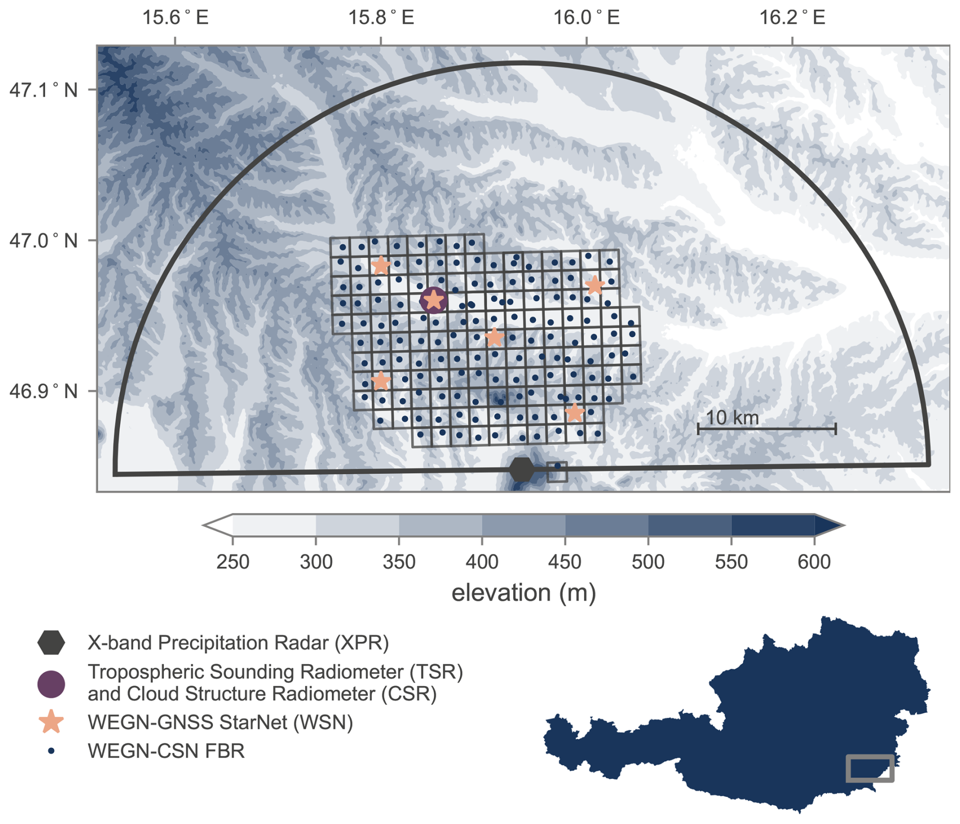
Figure 1 Sensor locations and horizontal coverage of the WegenerNet Climate Station Network (WEGN-CSN FBR) and the WegenerNet 3D Observing System in the Feldbach Region, which together form the WegenerNet 3D Open-Air Laboratory for Climate Change Research.

Fuchsberger et al. (2021)

Table 1 Sensor types and locations of the WegenerNet 3D Open-Air Laboratory (WEGN3D Open-Air Lab) infrastructure. The WEGN3D Open-Air Lab combines the 156 ground stations of the WegenerNet Climate Station Network Feldbach Region (WEGN-CSN FBR) and the WegenerNet 3D Observing System.

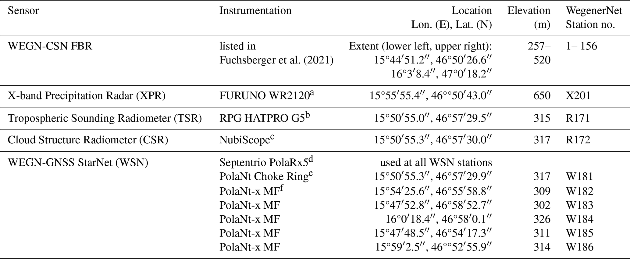
^a https://www.furuno.com/files/Brochure/456/upload/WR2120_en_1911.pdf (last access: 9 January 2026), ^b https://www.radiometer-physics.de/download/PDF/Radiometers/HATPRO/RPG_MWR_PRO-G5_TN 2022.pdf (last access: 9 January 2026), ^c http://nubiscope.eu/ (last access: 9 January 2026), ^d https://www.septentrio.com/en/products/gnss-receivers/gnss-reference-receivers/polarx-5 (last access: 9 January 2026), ^e https://www.septentrio.com/en/products/antennas/polant-chokering (last access: 9 January 2026), ^f https://www.septentrio.com/en/products/antennas/polant-x-mf (last access: 9 January 2026).

The XPR is located to the south of the climate station network on the Stradnerkogel, one of the highest elevations in the region. This allows for a clutter-free radar data collection over the entire 30 km radar sweep. The radar only scans towards the north, where the climate station network is located (see Fig. 1) with an azimuth range of −90 to 90°. This trade-off between coverage and scan duration means that a full volume scan of the half-hemisphere can be completed within 2.5 min. In addition to raw dual-polarization base data, moments, and estimates for precipitation rate and precipitation amount, the dual-polarization observations also allow the classification of hydrometeors (Zrnić et al., 2001; Straka et al., 2000; Evaristo et al., 2013).

The WSN GNSS stations are strategically distributed within the climate station network in a nested two-star configuration to maximize the spatial coverage and to provide different horizontal resolution for cross-comparisons. Primary output of the WSN are tropospheric path delay in zenith and slant direction, tropospheric gradients (e.g., Teke et al., 2011), and integrated water vapor (IWV, Bevis et al., 1992). Each WSN GNSS station is co-located with a climate station to provide high-quality surface meteorological observations for a robust IWV retrieval. In addition, WSN station W185 is equipped with a dedicated meteorological sensor in close proximity to the GNSS antenna due to its height above ground of approximately 12 m. Near real-time processing of the raw GNSS tracking data into tropospheric data variables is performed by the German Research Centre for Geosciences (GFZ), which processes such data for a large number of globally distributed GNSS stations (Ning et al., 2016; Wilgan et al., 2022).

The CSR continuously observes brightness temperatures in the 8 to 15 µm band. The high temperature contrast between clouds and clear sky allows the determination of cloud cover from an all-sky scan (e.g., Smith and Toumi, 2008). Combining the brightness temperature of detected cloud pixels with a temperature profile further enables the retrieval of cloud base heights and subsequently the generation of a 3D cloud structure (Brede et al., 2017).

The primary outputs of the TSR are all-sky scans and zenith observations of IWV, cloud liquid water path (LWP), and tropospheric path delay in addition to profiles of temperature and humidity. These quantities are the result of statistical retrieval algorithms based on observed microwave brightness temperatures (Crewell et al., 2001). These statistical retrievals are implemented using feed-forward neural networks (e.g., Jung et al., 1998) trained on reanalysis data for the specific sensor location. The numerical values of the network coefficients, offset, and scaling factors are provided by the instrument manufacturer. The TSR is also equipped with an infrared pyrometer extension whose pointing is coupled with the scanning parabola mirror of the microwave instrument. Consequently, the TSR also provides all-sky scans and zenith direction measurements of infrared brightness temperatures, albeit within the narrower 9.6 to 11.5 µm band.

Both radiometers are situated near the center of the climate station network at a designated radiometer site with the station identifiers R171 and R172. The radiometer site is located on top of a commercial building, approximately 30 m above ground in the Raab River valley, resulting in minimal viewing obstructions even at low elevations. The site is also co-located with the WSN station W181 which allows for cross-evaluation of selected data variables such as tropospheric path delay and IWV.

3 Data product overview

Each WEGN3D v1.0 data product is defined by a processing level, a product category, and a data product subcategory. Processing levels indicate the amount of processing steps involved in generating the data product and are discussed in detail in Sect. 3.1. Product categories specify the general theme of the data variables within the product, and product subcategories allow for refinement of the categorization by measurement domain and temporal resolution. For example, the data product WN3D_L1b_v1_MWR_SkyMaps contains data variables resulting from microwave radiometry (MWR) all-sky scans (sky maps) of the tropospheric sounding radiometer, while WN3D_L1b_v1_IRR_TimeSeries contains measurement time series derived from infrared radiometry (IRR) of the cloud structure radiometer. Level 2 data products are similarly named, for instance, WN3D_L2_BD_v1_Precipitation contains data variables related to precipitation in their highest temporal resolution, called basis data (BD).

Table 2 List of data products available as part of the WEGN3D v1.0, their processing level, product category, product subcategory, spatio-temporal domain, time resolution and key observables. The column “Key observables” lists selected measured or derived quantities, which target the primary science objectives of the WEGN3D Open-Air Lab. A detailed list of data variables can be found in Appendix A.

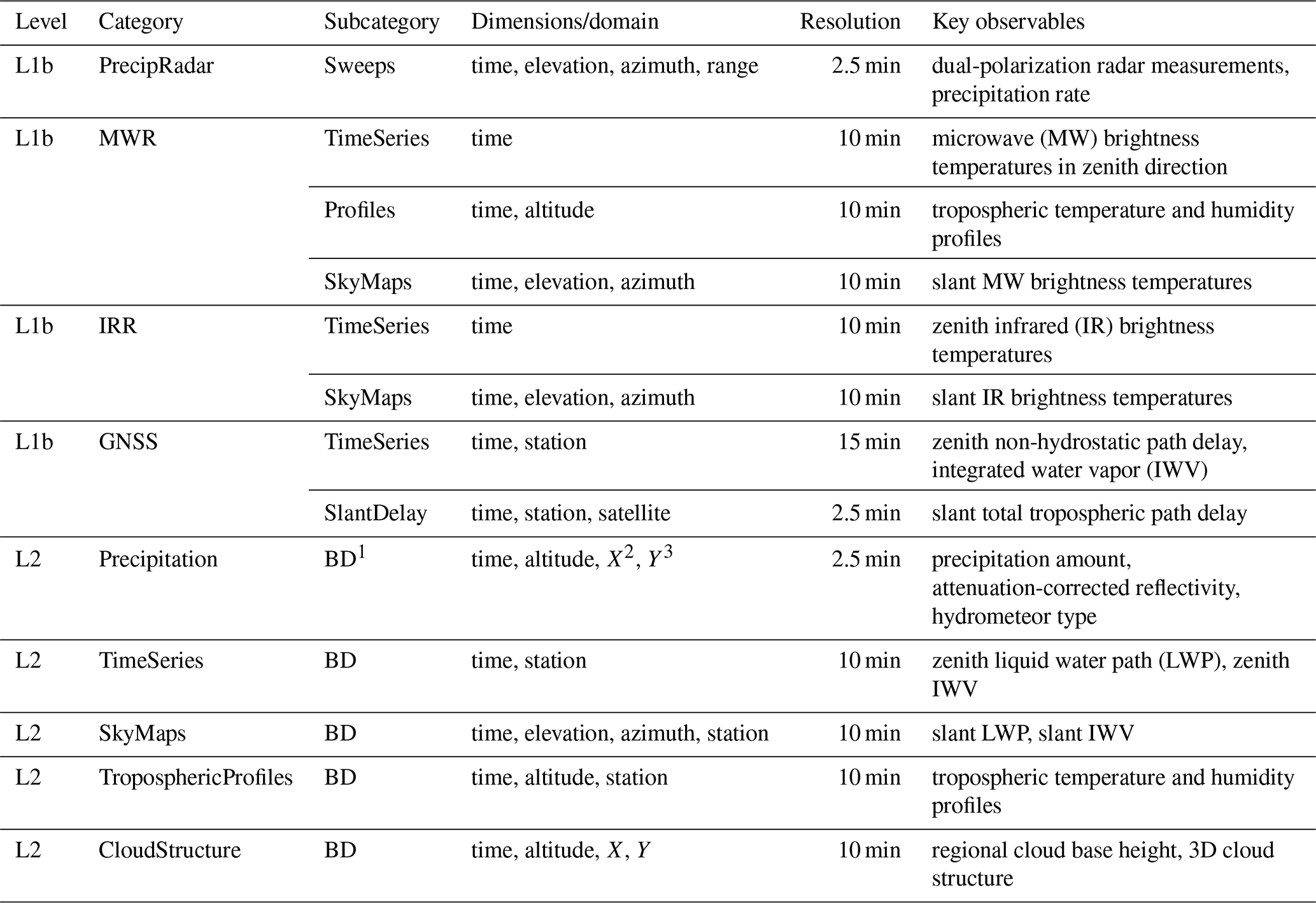
¹ Basis data, ² easting, ³ northing.

A complete list of all data products released in WEGN3D v1.0, can be found in Table 2.

In terms of observed physical variables, they can be divided into four thematic groups related to the essential climate variables precipitation, upper-air water vapor, clouds, and upper-air temperature as defined by the Global Climate Observing System (GCOS, Spence and Townshend, 1996; World Meteorological Organization (WMO) et al., 2022). In addition, data variables related to atmospheric stability including stability indices such as convective available potential energy (CAPE) and boundary layer depth are also included within the data products. A complete list of variables contained in the Level 1b and Level 2 data cubes, categorized by essential climate variable, is given in Appendix A.

3.1 Processing level definitions

The WegenerNet 3D Open-Air Lab data products are organized at the top level into a series of processing levels. These processing levels range from raw sensor data (Level 0), over consolidated and aggregated data (Level 1a/Level 1b) to geolocated and gap-filled atmospheric data cubes (Level 2).

Level 0 data (L0) are unchecked raw data in their native file formats, generated by the sensor software, data loggers, or are obtained from external sources. No post-processing steps are applied to L0 data, thus they are preserved in the state in which they are retrieved from the different sensors. Consequently, time resolution and reference frame definitions are not consolidated and can be expected to differ.

Level 1a data (L1a) are unchecked raw data in a consolidated storage format, that preserves native spatial and temporal resolutions. Measured quantities are renamed to common variable definitions and their units are adapted accordingly. No destructive processing (e.g., aggregation or averaging) is applied in the generation of L1a data, except for discarding incomplete or malformed input files or data records. As a result, L0 and L1a data have the same information content. L1a product files are temporarily stored in NetCDF format and follow the CF conventions (Hassell et al., 2017), version 1.7. Due to the considerable data volume, L0 and L1a data are made available upon request only.

Level 1b data (L1b) are resampled and/or aggregated to even timestamps in Coordinated Universal Time (UTC) at the product target resolution. L1b data products are grouped by sensor type and are given in (local) sensor reference frames. All data variable names and corresponding units are carried over from the L1a data. Additionally, the WegenerNet 3D Quality Control System (QCS3D) performs quality checks on the data, and attaches flags indicating degraded data points as supplemental metadata variables.

Level 2 data (L2) are gap-filled and geolocated datasets given in well-defined spatio-temporal reference frames. Degraded data, as indicated by the respective quality flags set by QCS3D, are discarded and the resulting gaps in space and time are filled by interpolation where possible. Interpolated data points are indicated by interpolation flags so they can be easily identified and removed if desired. L2 data are sensor agnostic and grouped by their spatio-temporal coverage or topical group, so no information about the underlying measurement system is required. They can be interpreted as the optimal observation of the respective physical variable from all available measurements. L2 data products are typically multi-sensor products, where either multiple sensors observing the same physical quantity are merged, or observations from different sensors are used to derive new target variables.

3.2 Data product coverage and resolution

The WEGN3D atmospheric data cubes are provided on grids that are a superset of the WEGN-CSN FBR Gridded Data Products version 8.0 (Fuchsberger and Kirchengast, 2023). The WEGN3D v1.0 base grid is defined in the UTM33N projection (EPSG code 32633, Nicolai and Simensen, 2008) with lower left cell coordinates of (539 800, 5 186 800 m), upper right cell coordinates of (602 600, 5 219 600 m), and a horizontal resolution of 200 m × 200 m. Height levels are defined relative to the mean sea level (AMSL), represented by the Austrian Geoid 2008 (Pail et al., 2009, 2008) and adequately cover the WEGN-3DO sensor resolutions. The detailed height levels used in the WEGN3D v1.0 atmospheric data cubes are listed in Table 3.

Table 3 Height level definitions along the vertical dimension of the WEGN3D v1.0 atmospheric data cubes.

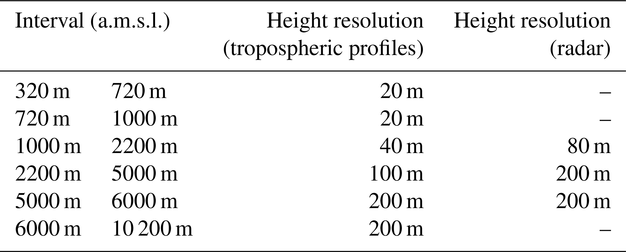
Radar-derived precipitation data products use a subset of these height levels in order to more accurately reflect the vertical resolution and information content of the underlying radar observations, while simultaneously reducing the data product storage size.

The temporal resolution of the L1b and L2 data products was chosen to be an integer multiple of the radar scan duration of 2.5 min to allow for easy aggregation into a common time series. Radiometer-derived datasets exhibit a temporal sampling of 10 min, which is the most common sampling among all data cubes. GNSS-derived L1b data are given as time series with a sampling of 15 min, which results from the GNSS processing chain currently employed at GFZ. However, since GNSS-derived L1b data are rather smooth in time due to the use of temporal constraints (e.g., Li et al., 2014), they are resampled to 10 min during the processing from L1b to L2 to be consistent with the other L2 products. The base sampling of 2.5 min also enables convenient comparisons through aggregation with the WEGN-CSN FBR L2 station time series and grid products (Fuchsberger et al., 2021; Fuchsberger and Kirchengast, 2023), which are given with a sampling of 5 min.

3.3 Data product versioning

Both WEGN3D Level 1b and Level 2 data products are expected to evolve over time, as their respective processing chains are optimized, improved quality checks are implemented, and new data variables are introduced. To ensure traceability for derived datasets and scientific use cases, each processing level is versioned according to the semantic versioning guidelines (https://semver.org, last access: 2 September 2024), albeit with adaptations tailored to data products. The primary deviation from the semantic versioning guidelines is that version numbers within WEGN3D datasets are restricted to major and minor version, with the possibility of adding descriptive labels for intermediate or experimental data product releases. This is primarily done to reduce complexity in the versioning scheme. Thus, all main data product releases that have been assigned a Digital Object Identifier carry a version number MAJOR.MINOR, which may be prefixed with a v for ease of identification, for example, v1.0. Special data releases, such as experimental processing chains or release candidates for evaluation and testing, are suffixed with a hyphen, followed by a descriptive identifier, as in v2.0-rc1.

As specified in the semantic versioning guidelines, how the version number is incremented depends on the nature of changes introduced into the processing chain. In general, small changes that do not change the meaning and content of output variables can be introduced during operational processing without a version increment. Historical data are not changed when such small housekeeping changes are introduced. To ensure traceability in this case, the software version used to create each data file is stored in its metadata via the corresponding Git commit hash.

The minor version of a dataset is incremented when changes unrelated to the data model are introduced. This means that the values of data variables change compared to the previous version while the data structure and metadata remains the same. This is typically the result of changes and improvements in the processing chain of existing data variables. A new minor version is expected to be a drop-in replacement for previous versions of the same major version release, and do not require the adaption of downstream software processing chains.

The major version of a dataset is incremented when backwards incompatible changes in a data product are introduced. Such changes may include different coordinate variable values, changes to variable or product names, or changes in variable units. A new major version is also expected to require software adaptions of downstream, user-implemented processing chains. Any minor or major version increment leads to a reprocessing of the whole time series to ensure a consistent data record based on the same processing chain.

4 Data processing and quality assurance

The WegenerNet 3D Processing System (WPS3D), is an extension of the WegenerNet Processing System (WPS, Fuchsberger et al., 2021), and forms the foundation for the generation of the WEGN3D v1.0 data cubes. In analogy to the WPS, WPS3D is split into modular application parts consisting of the Command Receive Archiving System (CRAS), which collects raw data from the distributed sensors, the 3D Quality Control System (QCS3D), which is responsible for quality checks and L1b generation, and the 3D Data Product Generator (DPG3D), which generates L2 geolocated data products.

4.1 WPS3D processing steps and data flow

The CRAS, which is shared with the WPS, retrieves raw data from the different WEGN-3DO sensors, and saves the sensor- and manufacturer-specific data files in the WegenerNet storage infrastructure as level 0 (L0) data. As per definition of the L0 data, no processing is applied in this step.

The WPS3D Quality Control System (QCS3D) for the WEGN-3DO data follows the same principle as the already well established QCS system for the WEGN-CSN data. The output of QCS3D are daily L1b NetCDF files conforming to CF-1.7 standards and are targeted at experienced users who want to analyze individual sensor data. Missing epochs are filled with Not-A-Number (NaN) values, thus the user can expect that the L1b time series is complete and evenly sampled. A set of eight QCS3D layers are applied to L1b data and if a predefined condition indicating degraded data is met, a quality flag represented by a bitmask is set accordingly. This quality flag is then added to each L1b data product as metadata with the naming scheme 〈variable_name〉_qcs_flag. A description of the individual QCS3D layer checks can be found in Table 4.

Table 4 Description of 3D Quality Control System layer checks to identify degraded measurement data.

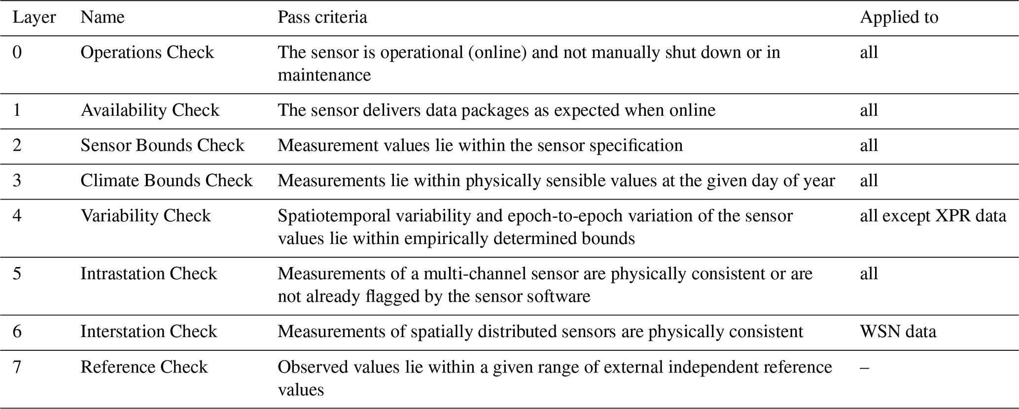
Layer 0 to Layer 3 are applied to the data simultaneously in a first step, whereas Layer 4 and higher are only applied to data points which pass the initial check. Due to the nature of the WEGN3D sensors, not all QCS3D layers can be applied to all sensors. For example, layer 6 (interstation check) can only be applied to WSN values because all other sensors and their output values are not directly comparable and are only located at a single station.

The WPS3D Data Product Generator (DPG3D) processes L1b data, taking into account quality flags assigned by the QCS3D. The general procedure is to drop degraded data, and fill resulting gaps by interpolation where reasonable. Interpolated values are indicated by a metadata variable following the naming scheme 〈variable_name〉_interp_flag. If resulting gaps exceed 24 h, values are replaced by either NaN or an appropriate integer fill value. L2 products are designed to be sensor agnostic and geolocated for easy comparison with other datasets, such as weather- and climate models.

An example of how a dataset is quality-checked by the QCS3D and then processed by the DPG3D, can be found in Fig. 2.

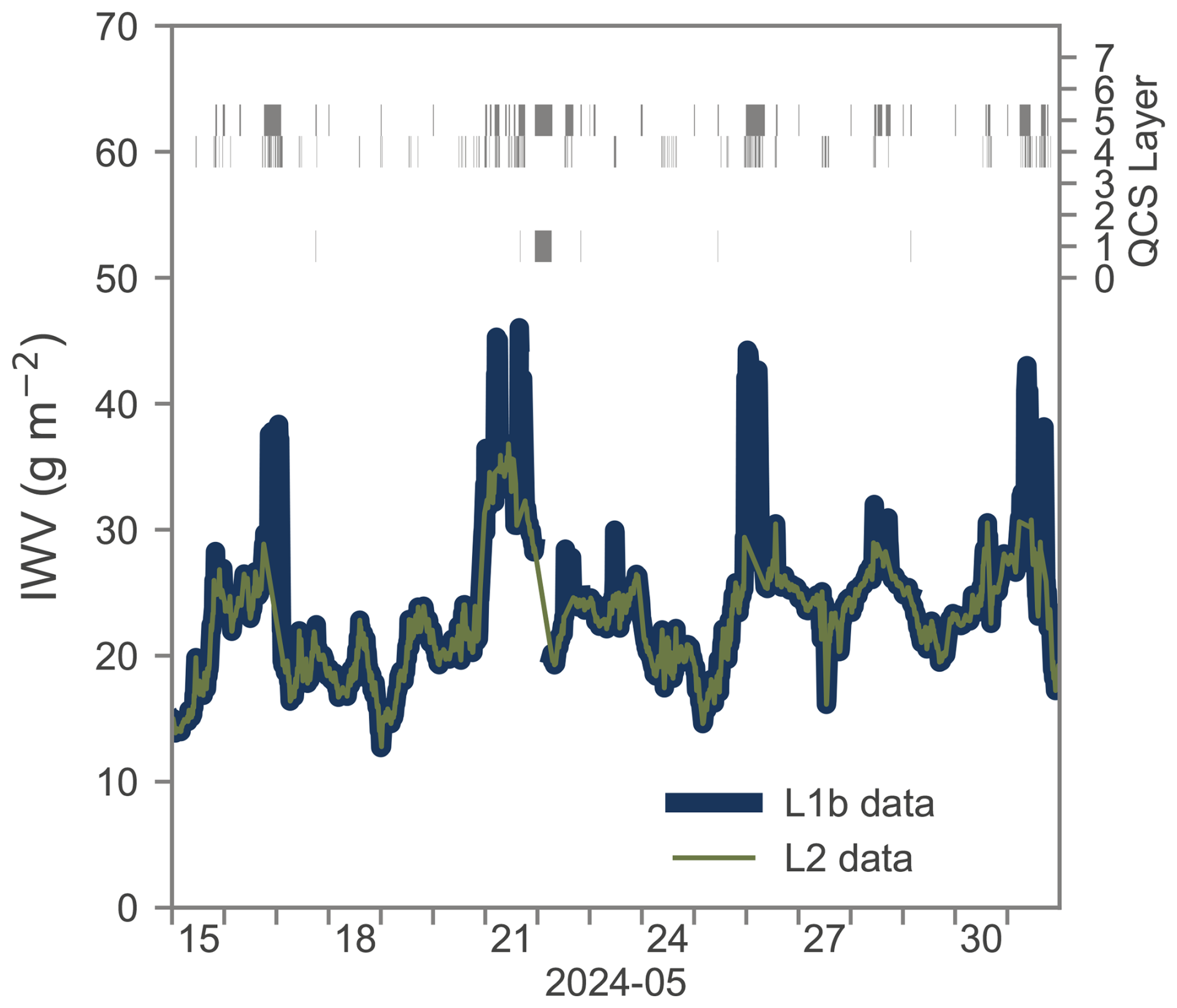
Figure 2 Comparison of L1b and L2 integrated water vapor (IWV) time series showcasing the QCS3D layer checks and their subsequent use in L2 processing to eliminate outliers and degraded data.

This example shows a time series of IWV in zenith direction as retrieved from microwave radiometry (MWR) by the TSR contained in the WN3D_L1b_v1_MWR_TimeSeries data product. As we can see, there are a number of spikes as well as periods with missing data which are flagged by the QCS3D. Spikes and jumps in the data are detected very well by QCS3D layer 4 (variability check), which compares the variability within a moving temporal window and the epoch-to-epoch variation with empirically determined upper and lower bounds. Exceedance of these thresholds results in the flagging of the corresponding epochs. QCS3D layer 5 (intrastation check) flags epochs where physically inconsistent observations occurred. For microwave radiometers this is typically the case during rainy conditions and when the radiometer membrane is covered by water (Wang et al., 2023; Ware et al., 2004), which results in drastic over- or underestimation of retrieved values. Checks for such events based on internal consistency and external rain gauge data are included in QCS3D layer 5, where periods during and after rainfall are flagged until the membrane can be considered dry again. DPG3D drops all data points where a single QCS3D layer detected degraded data and interpolates the resulting gaps, which results in a much smoother IWV time series without spurious spikes.

The full data processing flow from L0 data to L2 data products is schematically summarized in Fig. 3.

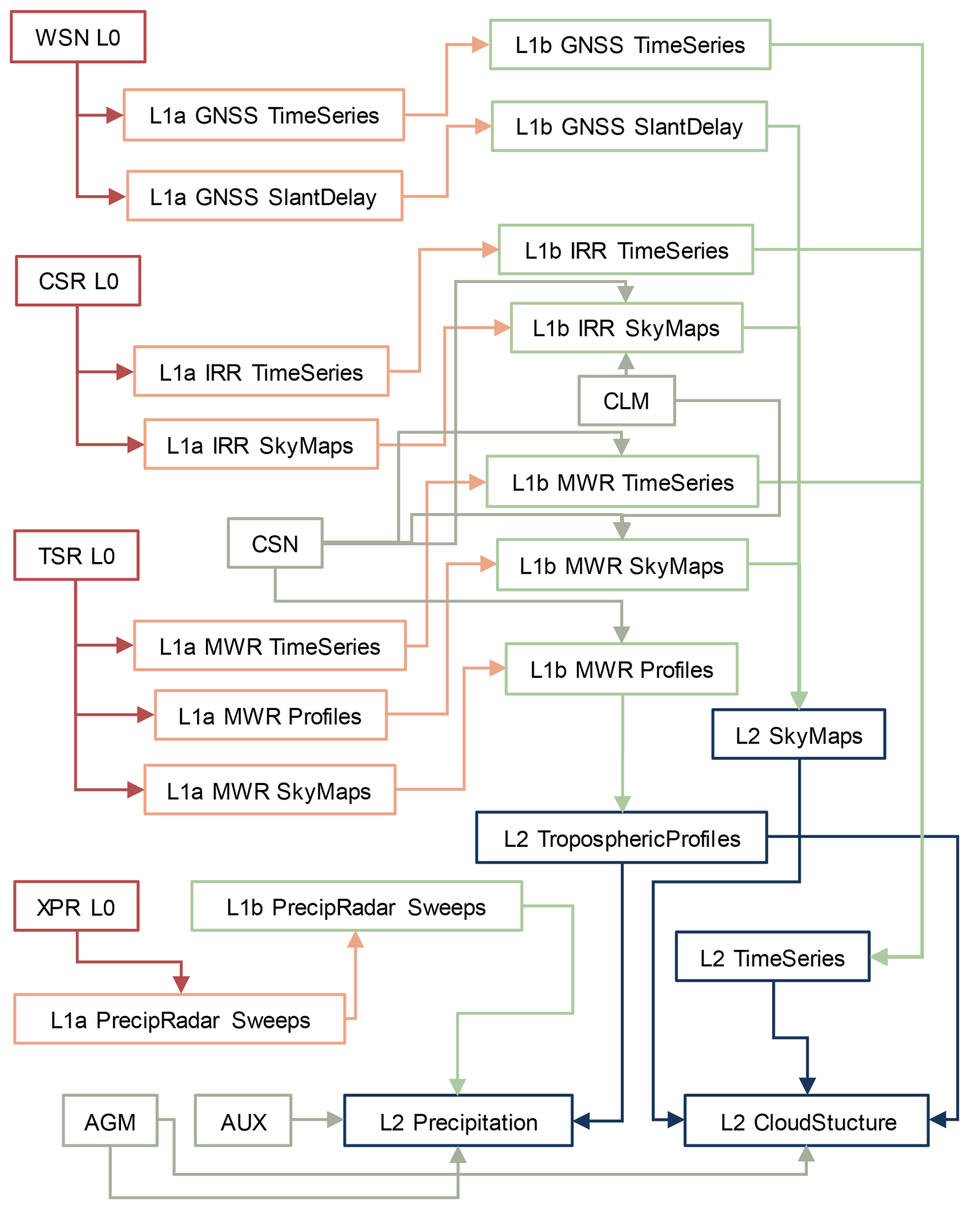
Figure 3 WegenerNet 3D Processing System data flow from X-band precipitation radar (XPR), cloud structure radiometer (CSR), tropospheric sounding radiometer (TSR), WEGN-GNSS StarNet (WSN) level 0 (L0) data, via L1a/L1b data, to level 2 (L2) data. The flowchart also shows where climate station network (CSN) data, auxiliary data (AUX), clutter maps (CLM) and geoid model (AGM) data are incorporated.

Throughout the processing steps, not only WEGN-3DO measurement data are used, but also meteorological measurements from the climate station network (CSN) and (static) auxiliary data. These auxiliary datasets include the Austrian Geoid Model 2008 (AGM, Pail et al., 2009, 2008) for the conversion between geometric height above the reference ellipsoid and height above the mean sea level (AMSL), clutter maps (CLM) to flag static obstructions in L1b sky maps, and classification model parameters for hydrometeor classification (AUX). CSN data are used in the computation of the sun position to flag potential sun intrusions in radiometer L1b sky maps. In general, the data processing flow from L0 data to L1b is sensor specific, that is, each sensor data stream is processed independently without using other instrument data. L2 data on the other hand are multi-sensor products in the sense that they either merge and consolidate different L1b data products (e.g., WN3D_L2_BD_v1_TimeSeries) or make use of other L2 data in their generation. That is, for example, the case for the WN3D_L2_BD_v1_Precipitation product where L2 tropospheric temperature profiles are used as supplementary data to assist in the hydrometeor classification.

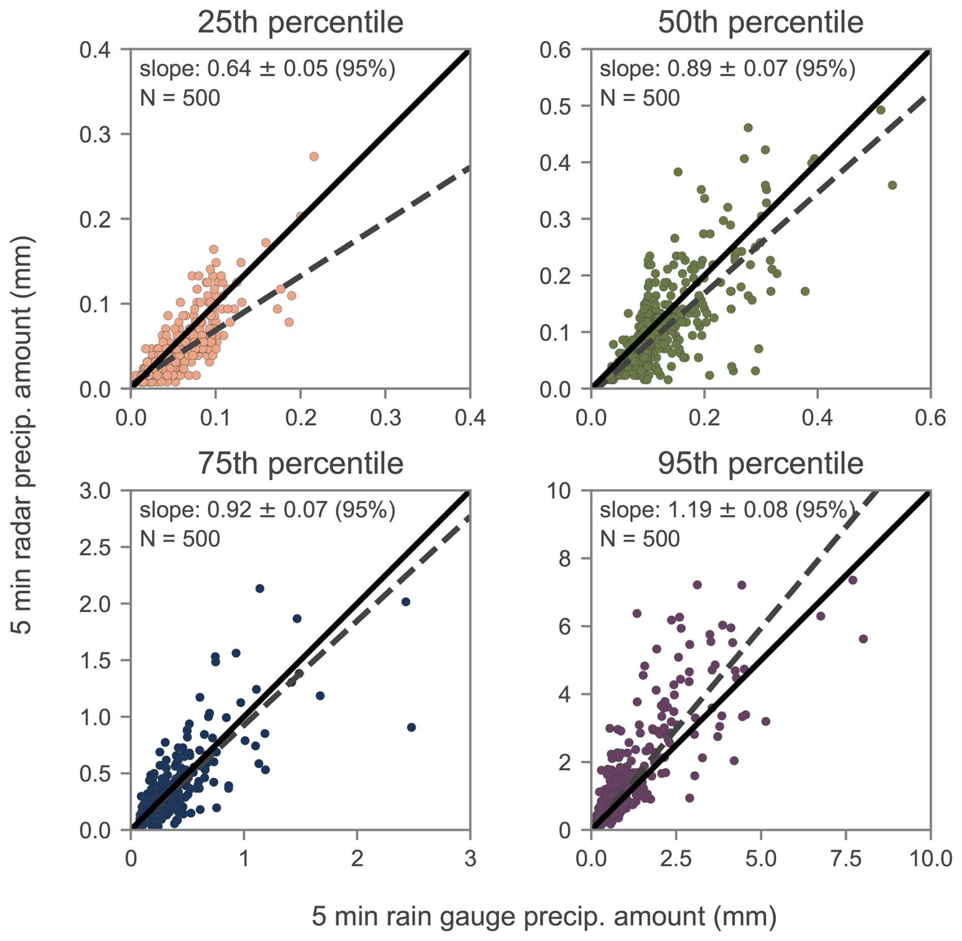
Figure 4 Event-based comparison of 5 min precipitation amount percentiles for gridded WEGN-CSN FBR L2 rain gauge data and time-aggregated WEGN3D v1.0 L2 precipitation fields at the lowest radar height level of 1 km a.m.s.l. (above mean sea level), subset to the spatial extent of the CSN grid. In this comparison, the 500 strongest events with respect to rainfall intensity were included.

4.2 Quality assurance outside of QCS3D

As stated in Table 4, QCS3D Layer 7 (reference check) is currently not used, as no external independent data source with sufficient accuracy, coverage, and resolution is available at the moment. Consequently, proper sensor maintenance, regular sensor calibration, and intersensor consistency checks are crucial to ensure a high level of data quality and consistency.

One cross-check for WEGN3D v1.0 data products is performed by comparing radar-derived precipitation amounts with those of the dense rain gauge network of the WEGN-CSN FBR. Our goal here is to see whether general under- or overestimation of the precipitation amount between the two independent measurement systems occurs.

Figure 4 shows the 25th, 50th, 75th, and 95th 5 min precipitation amount percentiles computed for the 500 strongest precipitation events with respect to rainfall intensity. The larger radar grid was subset to the spatial extent of the rain gauge network for a consistent comparison. Both 50th and 75th percentile show a good agreement between radar-derived precipitation amount and rain gauge measurements with a correlation close to 1, while for the 25th and 95th percentile we see under- and overestimation respectively. We attribute this to the higher spatial resolution of the radar-derived precipitation fields, which can resolve smaller-scale features compared to the rain gauge network with an interstation-distance of about 1.4 km and thus produce longer tails in the empirical distribution.

We perform absolute calibrations of the TSR twice a year according to the manufacturer's recommendations. Relative calibrations of the instrument are performed with each measurement cycle resulting in a 10 min relative calibration interval. The co-located WSN station W181 enables a direct comparison of quantities observed by both techniques, such as integrated water vapor (IWV). GNSS-derived water vapor can be considered homogeneous in time, as long as the processing chain and site instrumentation do not change (Van Malderen et al., 2020), and thus serves as an external stability check for the radiometer observations.

Figure 5 shows the comparison between WSN- and TSR-derived IWV. We can see that the radiometer observes higher IWV values compared to the WSN station W181 with an offset of 1.12 kg m⁻² and a drift of (0.16±0.02) kg m⁻² yr⁻¹ (95 % CI). These offset and drift values were estimated using the robust Theil–Sen estimator (Theil, 1992; Sen, 1968). The estimated radiometer trend (0.66±0.03) kg m⁻² yr⁻¹ (95 % CI) also stands out when compared to the other WSN stations, which exhibit positive IWV trends in the range of 0.23 to 0.53 kg m⁻² yr⁻¹ with a similar confidence interval. While this is negligible for studies of hydrometeorological extreme events, it will become relevant once the measurements' temporal coverage is sufficiently long for trend analysis and is currently under investigation. It is also evident that absolute calibrations do not substantially influence the GNSS-radiometer offset with monthly offset differences below 0.3 kg m⁻², which suggests a generally homogeneous measurement system.

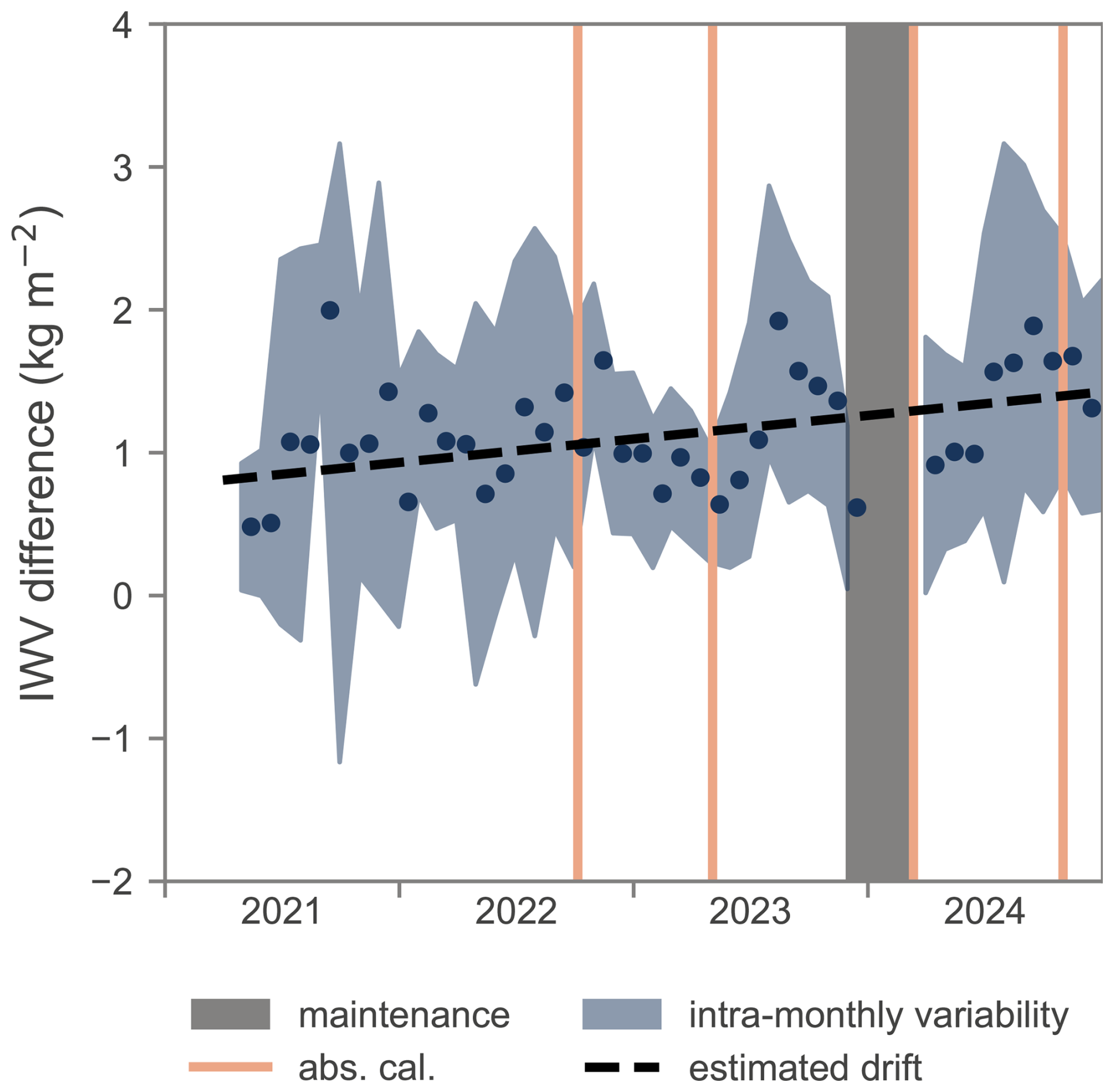
Figure 5 Comparison of month-to-month variation of radiometer-derived and GNSS-derived integrated water vapor (IWV) differences (dots) with the intra-monthly variability envelope. The four vertical lines indicate when absolute radiometer calibrations took place, while the shaded time span during winter 2023/2024 indicates instrument maintenance.

The co-located cloud structure radiometer (CSR) and tropospheric sounding radiometer with its infrared radiometer extension (TSR-IRR) allow a comparison of the observed infrared brightness temperatures (BRTs) and derived cloud base heights (CBH). It should be noted that these IR radiometers measure different bandwidths, namely in the 8 to 15 µm band (CSR) and in the 9.6 to 11.5 µm band (TSR-IRR), respectively, so a different response to the downwelling thermal radiation for very thin clouds can be expected. We therefore exclude BRTs and CBHs where the corresponding liquid water path retrieval is below 50 g m⁻² in comparisons between the two instruments. In Fig. 6a we can see that the TSR-IRR observes lower BRT indicated by a significant bias of ($-\mathrm{0.82}\pm \mathrm{0.15}$) K (95 % CI). Consequently, the derived CBHs are higher with a bias of (0.17±0.03) km (95 % CI) as shown in Fig. 6b. The CBH overestimation of the TSR-IRR compared to the CSR is accentuated for higher clouds, indicated by the significantly positive slope.

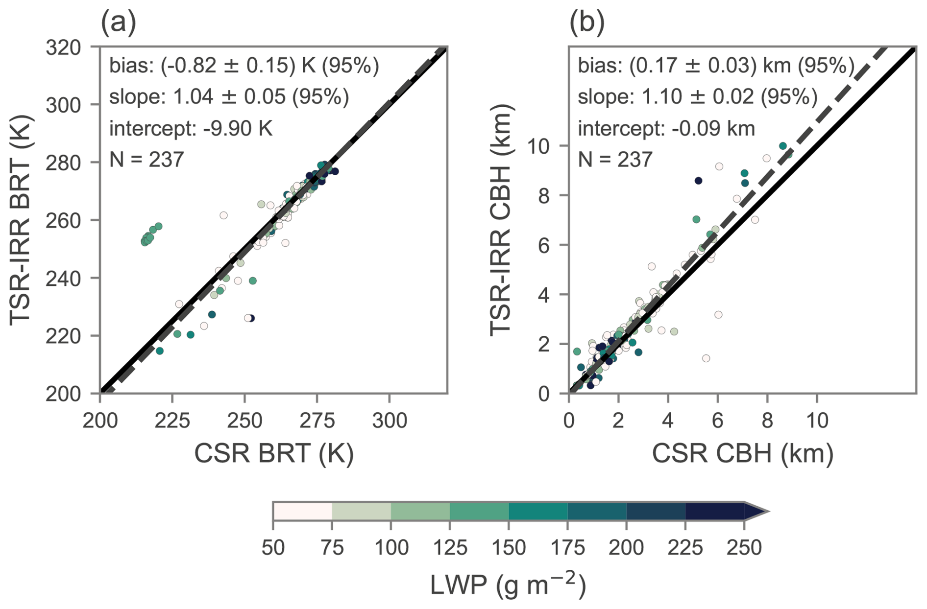
Figure 6 Comparison of hourly zenith infrared brightness temperatures (BRT) and cloud base height (CBH) averages between the cloud structure radiometer (CSR, 8 to 15 µm band) and the infrared extension of the tropospheric sounding radiometer (TSR-IRR, 9.6 to 11.5 µm band) sampled between September 2021 and April 2024: (a) scatter plot of infrared BRT and (b) scatter plot of derived CBH. Pairs are color coded by the corresponding hourly zenith liquid water path (LWP) averages to identify thin clouds. The color theme for LWP follows Thyng et al. (2016).

However, these characteristics are stable in time as both BRT differences and CBH differences exhibit insignificant temporal drifts of (0.07±0.25) K yr⁻¹ (95 % CI) and ($-\mathrm{6}\pm \mathrm{12}$) m yr⁻¹ (95 % CI) respectively.

These intersensor consistency checks are performed when significant changes to the processing chain are implemented, when a new data product release candidate is prepared, or when changes to the instrumentation are made, for example, sensor changes, maintenance and calibrations.

5 Example science use case

One of the many useful science applications of the WEGN3D Open-Air Lab is the observation-driven life cycle analysis of heavy precipitation events. We have selected such an exploratory analysis for an event of interest as an example case to demonstrate the science utility of the new dataset. In terms of typical meteorological conditions, the WegenerNet FBR is well suited for these studies because convective precipitation occurs frequently during the warm season (April to September, Schroeer et al., 2018; Haas et al., 2024), often accompanied by thunderstorms (Taszarek et al., 2019) and hail (Hulton and Schultz, 2024; Giordani et al., 2024). From mid-2020 to (including) 2024, we recorded 1522 precipitation events, of which 608 were classified as convective or a combination of stratiform and convective. 77 events exhibit rainfall intensities above 100 mm h⁻¹, and in 45 of these events, the radar-based hydrometeor classification detected hail.

The data variables within the WEGN3D v1.0 dataset can track key characteristics of precipitation events from formation to dissipation. To illustrate how selected L2 data products may be used to study these precipitation events without the need for extensive post-processing, we focus on a strong convective event that occurred on 15 September 2022. In this event we observed rainfall intensities exceeding 200 mm h⁻¹ within a very narrow rain band traversing the WEGN3D Open-Air Lab in east-southeast direction. Figures 7–9 showcase precipitation, water vapor, and cloud properties before, during, and after the event.

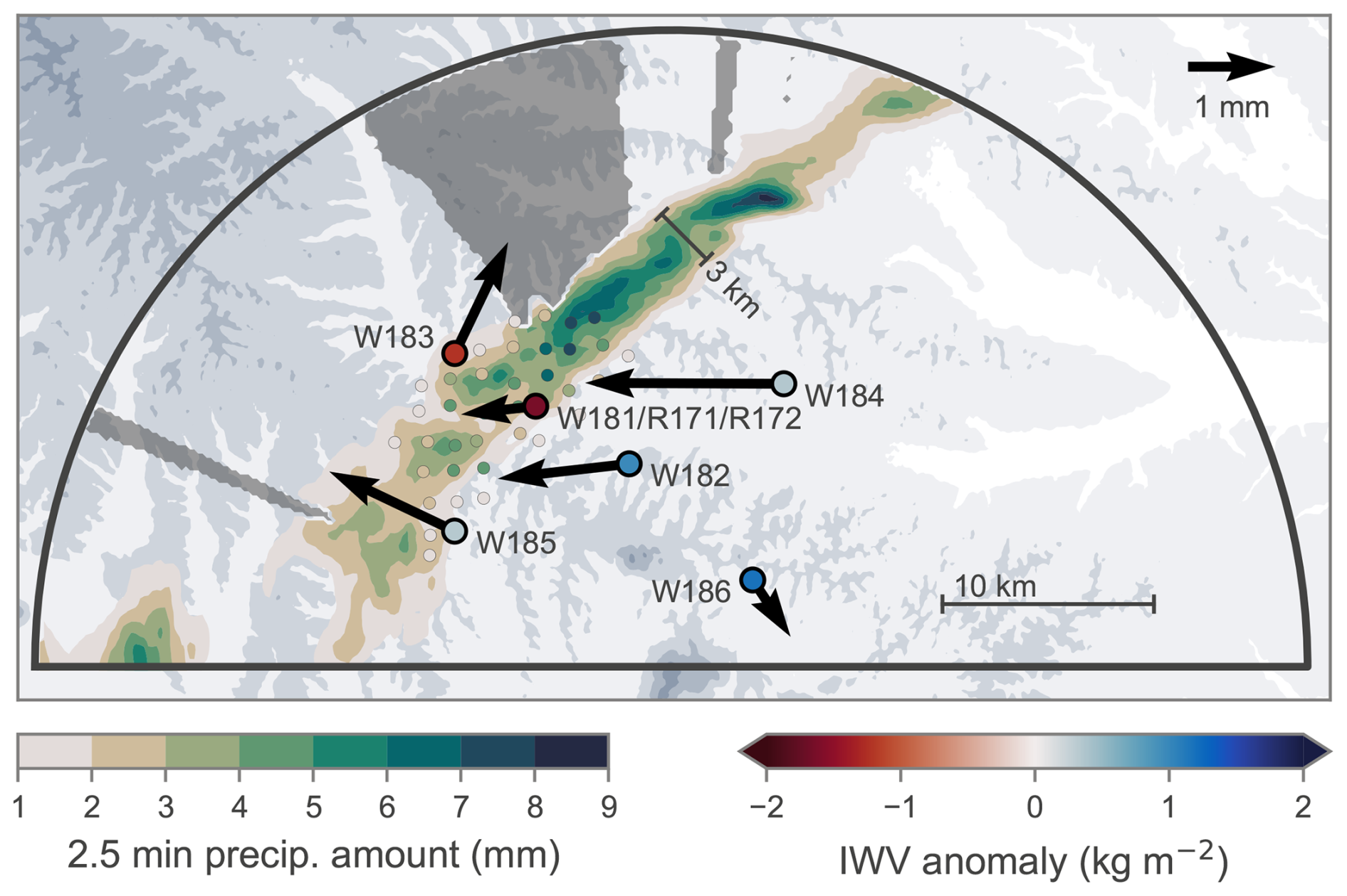
Figure 7 Snapshot of precipitation amount (radar-derived and rain gauge), regional integrated water vapor (IWV) anomaly, and GNSS-derived tropospheric gradients at the precipitation maximum (11:42:30 UTC) during a precipitation event on 15 September 2022. The arrows depict the estimated gradient direction and magnitude. The small circles show the 5 min rain gauge measurements of the climate station network, scaled to match the 2.5 min radar accumulation period (rain gauges with measured precipitation below 1 mm are omitted). Gray shaded areas indicate severely attenuated radar signals. Color schemes for precipitation amount and IWV follow Thyng et al. (2016).

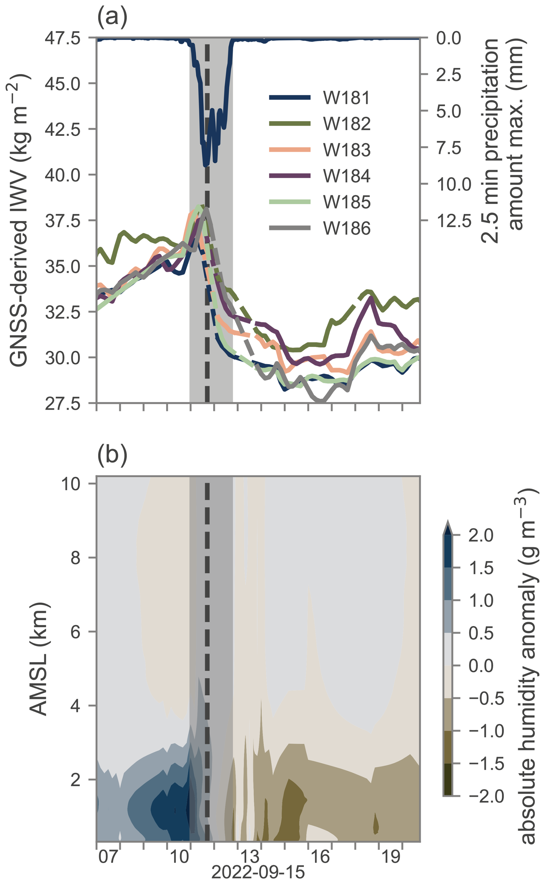
Figure 8 Temporal evolution of water vapor before, during, and after the precipitation event on 15 September 2022: (a) GNSS-derived integrated water vapor (IWV, dashed lines indicate interpolated data) and (b) radiometer-derived absolute humidity anomaly profiles. The shaded area depicts the event duration, while the dashed vertical line indicates the time of the precipitation maximum. The color scheme for the absolute humidity anomaly follows Thyng et al. (2016).

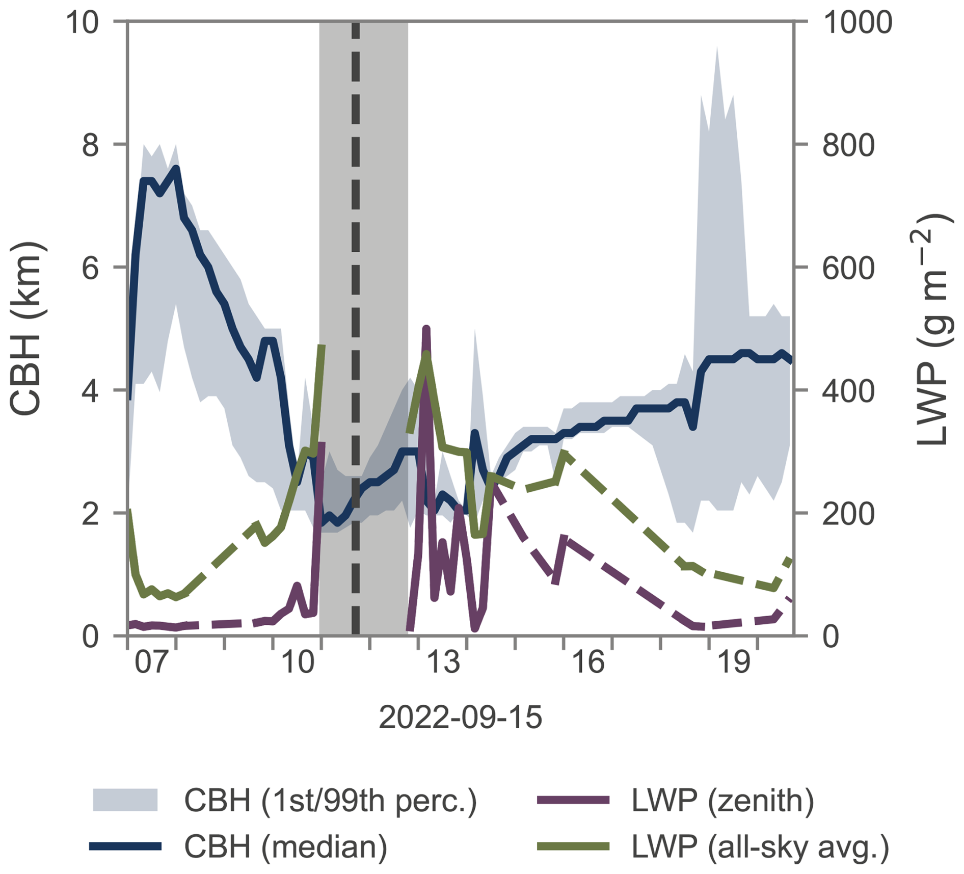
Figure 9 Temporal evolution of liquid water path (LWP, dashed lines indicate interpolated data) and cloud base height (CBH) before, during, and after the precipitation event on 15 September 2022. The shaded area depicts the event duration, while the dashed vertical line indicates the time of the precipitation maximum.

In Fig. 7 we can see the interaction between radar-derived precipitation amount, rain gauge measurements, GNSS-derived tropospheric gradients, and GNSS-derived IWV. Note that the rain gauge measurements exhibit a temporal resolution of 5 min compared to the 2.5 min radar resolution and thus cannot fully localize the fast-moving rain band. The spatial IWV anomaly follows the spatial structure of the rainfall, with lower IWV values in areas where rain has already started and higher IWV values in the travel direction of the rain band.

Tropospheric gradients are also related to convective precipitation (e.g., Brenot et al., 2013) as they indicate areas with atmospheric instability. The short baselines of the WEGN-GNSS StarNet in combination with the high-resolution precipitation fields will allow to study this behavior in more detail.

The temporal evolution of water vapor is shown in Fig. 8.

We can see an increase in IWV before the event, with a drop following the precipitation maximum (Fig. 8a). This is mirrored by the absolute humidity anomaly profiles shown in Fig. 8b, which exhibit a sharp increase below 2 km in the hours before the precipitation event, followed by strong negative anomalies afterwards.

The cloud parameter time series depicted in Fig. 9 show an increase in liquid water path (LWP) before the occurrence of precipitation, coupled with a decrease in the regional cloud base height (CBH). We can also observe the cloud structure becoming more consistent, as the range of the CBH becomes smaller. LWP fluctuates around approximately 100 g m⁻² in the hours after the precipitation event, before it decreases. The comparison of zenith LWP with the all-sky LWP weighted averages allows the distinction between local and regional cloud conditions.

6 Data availability

WEGN3D v1.0 L1b data (Kvas et al., 2024a, https://doi.org/10.25364/WEGC/WPS3D-L1B-10) and L2 data (Kvas et al., 2024b, https://doi.org/10.25364/WEGC/WPS3D-L2-10) are available under the Creative Commons Attribution 4.0 International (CC BY 4.0) license and are published on the WegenerNet Data Portal (https://wegenernet.org/portal/3ddownload/, last access: 9 January 2026). The WegenerNet Data Portal offers several methods to retrieve the data files, including an application programming interface (API) that allows the direct download of individual data product NetCDF files or subsets thereof (https://wegenernet.org/data-api/file/v1/api/, last access: 9 January 2026). Moreover, an alpha version of the Open Geospatial Consortium (OGC) Environmental Data Retrieval (EDR) API (https://wegenernet.org/data-api/ods/v0/api/, last access: 9 January 2026), which allows easy integration into existing services and applications due to its standardized nature, is also available. In addition, the WegenerNet Data Portal features web user interfaces for subsetting and bulk downloads for convenient manual data selection.

7 Conclusions

The first release of the WEGN3D Open-Air Lab atmospheric data cubes (WEGN3D v1.0 dataset) extends the already well established climate station network datasets (e.g., Fuchsberger et al., 2021) in the WegenerNet Feldbach Region with high-resolution atmospheric measurement data from the surface to the upper troposphere. The data cubes comprise essential atmospheric variables related to precipitation, cloud structure, atmospheric water vapor, upper-air temperature, and atmospheric stability at sub-kilometer scale and sub-hourly temporal resolution. The datasets are continually extended in time with the goal to provide a consistent long-term observational data collection. They are very well suited for the evaluation and validation of numerical weather prediction models, atmospheric reanalyses, high-resolution regional climate models, and remote sensing satellite data. They further allow for the study of weather phenomena in a changing climate using rich observational information that helps to unveil process knowledge, and can support the evaluation and development of retrieval algorithms and processing methods such as quantitative precipitation estimation from radar data.

The WEGN3D atmospheric data cubes are a living dataset that will improve over time through advancements in the processing chain and quality control system; thus we employ a strict versioning scheme to ensure traceability for users of the dataset. All data cubes are published in self describing data formats and are publicly accessible through application programming interfaces (APIs) in addition to web interfaces for manual subsetting and download at the WegenerNet Data Portal (https://wegenernet.org/portal/3ddownload/, last access: 10 June 2025).

Appendix A: Topical grouping of data variables

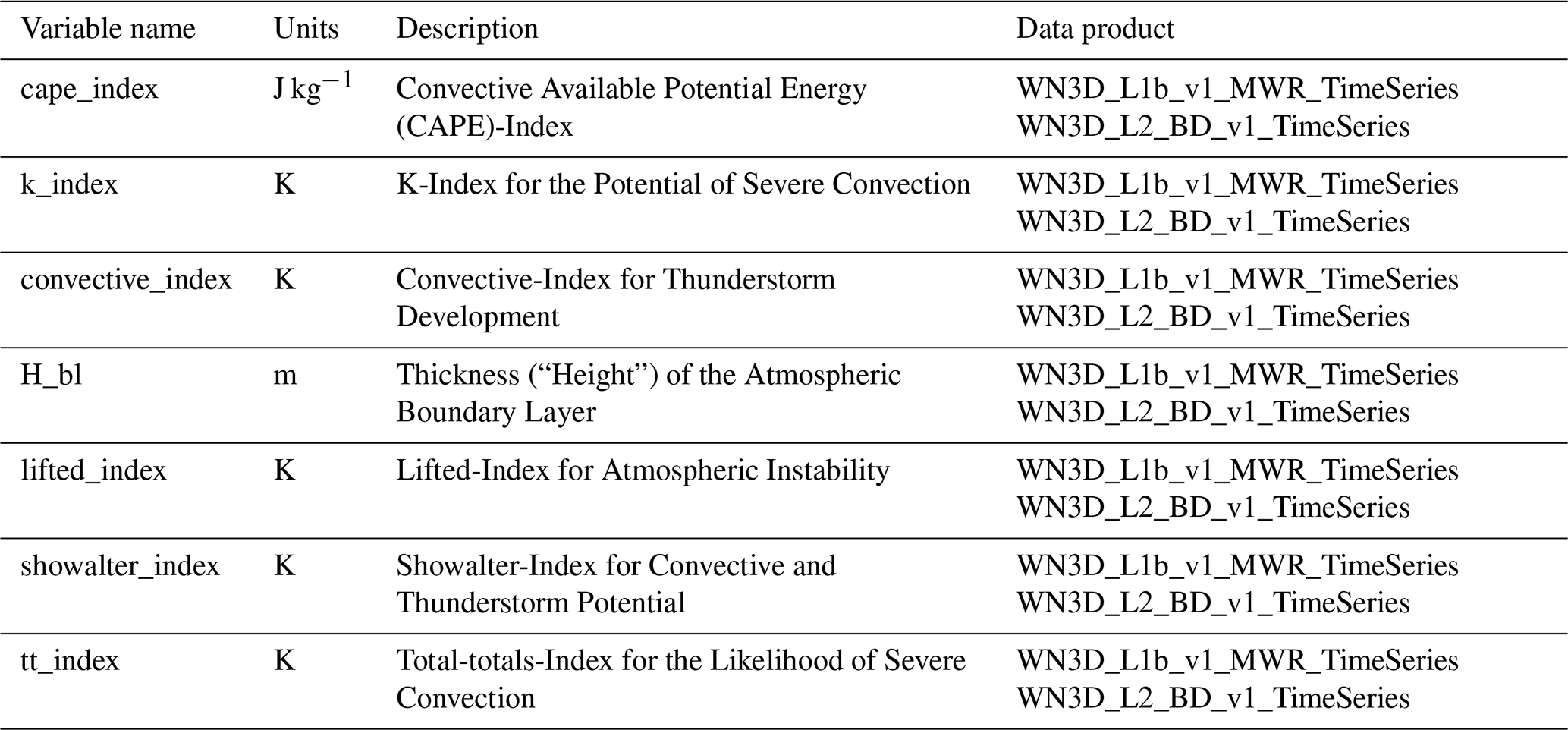
Tables A1 to A5 contain a topical grouping of all data variables contained within the WEGN3D v1.0 dataset. Data variables are grouped into the following essential climate variables (Bojinski et al., 2014) Precipitation (Table A1), Upper-Air Water Vapor (Table A2), Upper-Air Temperature (Table A3), and Clouds (Table A4). Additionally, the topical group Atmospheric Stability (Table A5) contains data variables related to vertical air motion and the atmospheric boundary layer. Note that data variables are listed once for each data product they are contained in and that data variables may be included in multiple topical groups.

Powell et al. (2016)

Table A1 List of data variables and their description in the topical group “Precipitation”.

Table A2 List of data variables and their description in the topical group “Upper-air Water Vapor”.

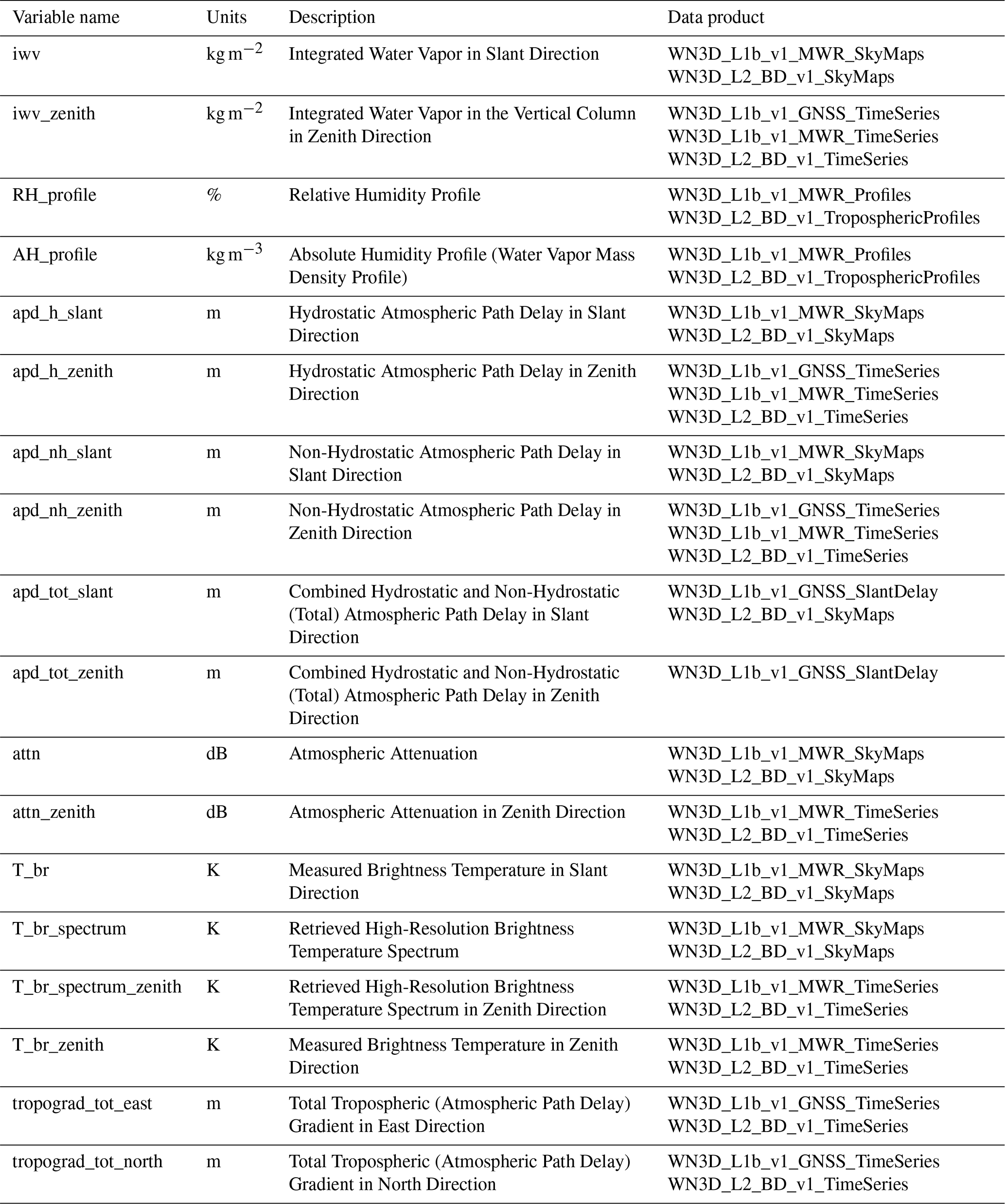
Table A3 List of data variables and their description in the topical group “Upper-air Temperature”.

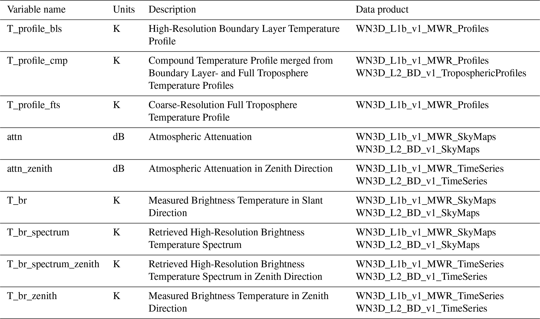
Table A4 List of data variables and their description in the topical group “Clouds”.

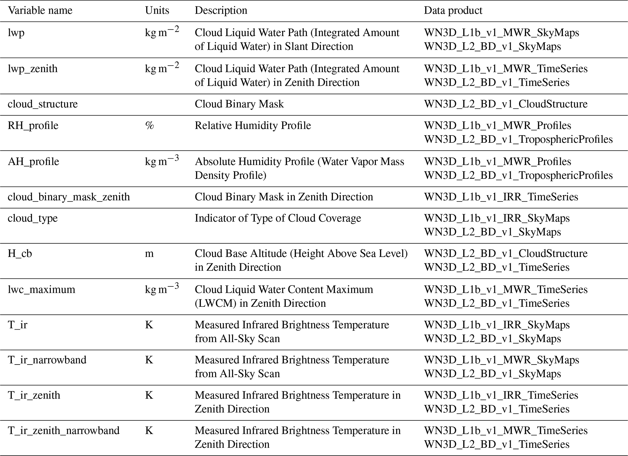
Table A5 List of data variables and their description in the topical group “Atmospheric Stability”.