Surface current variability in the East Australian Current from long-term high-frequency radar observations

The East Australian Current (EAC) exhibits significant variability across a wide range of spatial and temporal scales, from mesoscale eddies and meanders to seasonal, interannual, and long-term fluctuations in its intensity, pathway, and influence on the continental shelf circulation. Understanding and monitoring this variability is crucial, as the EAC plays an important role in controlling shelf dynamics, regional circulation, coastal weather, and global climate patterns. As such, two high-frequency (HF) coastal radar systems have been deployed on the eastern coast of Australia to measure surface currents upstream and downstream of the East Australian Current (EAC) separation point. The multiyear radar dataset (spanning 4–8 years) is presented here, and its use is demonstrated to assess the spatial and temporal variability in the EAC and the adjacent continental shelf circulation, ranging from seasonal to interannual scales. The dataset is gap-filled using a 2dVar approach (after rigorous comparison with the traditional unweighted least-squares (LS) fit method). Additionally, we explore the representation of the depth variability in the observations by comparing the data with surface Lagrangian drifter velocities (with and without depth drogues). The multiyear radar-derived surface current dataset, which was validated using short-term drifter and long-term current meter observations, revealed that the local upstream circulation is strongly dominated by the EAC's annual cycle, peaking in the austral summer. The analysis using 8 years of upstream data revealed the period of the EAC intensification at around 3–5 years. The interannual variability in the poleward transport downstream was driven by the intrinsic variability in the jet. This dataset which continues to be collected, complemented by numerical simulations and in situ measurements, will provide a comprehensive view of the EAC's variability and its impact on the broader regional circulation dynamics that can be used for a range of dynamical investigations. The datasets are freely available at https://doi.org/10.5281/zenodo.13984639 (Tran, 2024a).

1 Introduction

The southeastern Australian coastal zone is home to a diverse array of unique marine habitats and ecosystems and also offers substantial socioeconomic value through various maritime activities and industries. However, understanding and quantifying the complex dynamics that govern these regions poses a major scientific challenge (Roughan et al., 2015). One of the difficulties is that ocean motions exhibit intricate interactions across a vast range of spatial and temporal scales. This complexity is further amplified in shallow shelf regions, where the currents and circulation patterns exhibit significant variability driven by a wide spectrum of external forcing mechanisms. These give rise to intricate flow patterns (e.g., frontal eddies and filaments) and physical processes that are inherently difficult to observe and quantify through conventional means (Simpson and Sharples, 2012).

Owing to this challenge, considerable work has been invested to extend the capacity of the ocean observation network. In recent years, high-frequency (HF) coastal radar has become an important part of coastal ocean observing systems and is recognized as an efficient tool for studying and monitoring coastal regions (Roarty et al., 2019). HF radar is a remote-sensing technique that measures surface ocean currents and waves from the shore. The HF radar interprets surface currents by analyzing the backscattering of radar-emitted signals, known as “backscatter”. These backscatters are induced by the surface ocean ripples from long wind-generated waves (with wavelengths ranging from 3 to 30 m) in the ocean. Based on an analysis of the spatially and temporally varying radar signal, information on the sea surface wind, waves, and currents can be obtained (Paduan and Washburn, 2013). The advantage of the HF radar comes from its ability to continuously monitor surface currents and waves at high frequency across a wide area up to hundreds of kilometers offshore. This advantage of HF radar plays a crucial role in improving the observation capacity: it effectively bridges the gap between continuous and local measurements obtained via in situ methods (such as mooring observations) and the broader but less frequent satellite data. By combining radar measurements with other techniques, the HF radar data provide a comprehensive description of surface currents, from hourly to interannual variations.

By way of example, several studies using HF radar have occurred in recent years, such as the analysis of long-term variation in the Soya Warm Current (Ebuchi et al., 2009), seasonal shifts in the western United States coastal shelf circulation (García-Reyes and Largier, 2012), variability in the East Australian Current (Archer et al., 2017a), Florida current (Archer et al., 2017b), variability in the Gulf Stream (Muglia et al., 2022), and comparison studies between systems (Archer et al., 2018). Other applications include focusing on dynamic features, such as small eddies (Mantovanelli et al., 2017; Schaeffer et al., 2017); marine renewable energies; wind–wave interaction (Ardhuin et al., 2009; Dzwonkowski et al., 2009; Thiébaut and Sentchev, 2016; Schaeffer et al., 2020); and detecting rapid current variations, providing crucial data for navigation, search and rescue operations, and environmental monitoring (e.g., Klinger et al., 2017).

Off the eastern coast of Australia, the East Australian Current (EAC), a highly dynamic western boundary current of the subtropical South Pacific Gyre, plays an important role in the marine ecosystem and climate of the region (Fig. 1a). It redistributes heat, marine organisms, nutrients, and debris while also moderating weather patterns and climate dynamics by transporting warm subtropical waters poleward toward the temperate midlatitudes. On a local scale, the EAC significantly influences shelf dynamics in multiple ways (Schaeffer et al., 2014, 2017; Malan et al., 2023). Originating between 10 and 20° S, the EAC strengthens, meanders consistently, and flows southward along the coast, carrying an average transport of about 22 Sv. It eventually separates at around 30–32° S, transitioning into an eastward flow known as the Tasman Front, and a field of southward-propagating eddies extend poleward (Oke et al., 2019). According to the literature (Kerry and Roughan, 2020; Cetina-Heredia et al., 2014), the EAC intensifies and separates from the coast between 31 and 34° S and between 32 and 33.5° S 38 % of the time. The EAC remains attached to the coast from its origin around 18° S until about 32° S, where part of the jet separates from the coast, shedding eddies that flow eastward and form the EAC eastern extension and those that continue southward and form the EAC southern extension (Oke et al., 2019). The southern extension pathway of the EAC can be recognized from the multiyear mean circulation pattern in Fig. 1a, which shows that the poleward velocity at Newcastle is half as strong as the velocity at Coffs Harbour. The EAC, like other western boundary currents, plays a crucial role in the oceanic circulation system.

In this regard, the HF radar has been deployed as part of the effort to monitor the East Australian Current (EAC). HF radar was first deployed off Coffs Harbour, southeastern Australia, in March 2012 by Australia's Integrated Marine Observation System (IMOS; Table 1). Since then, HF radar observations have been used to advance our understanding of the regional dynamics and variability in the EAC (e.g., Archer et al., 2017a; Mantovanelli et al., 2017; Malan et al., 2023; Schaeffer et al., 2017, etc.). Flowing near the narrow continental shelf, the EAC interacts with coastal topography, enhancing uplift and upwelling processes that replenish nutrients and maintain high biological productivity (Roughan and Middleton, 2004). The proximity of the EAC to the shelf creates intricate structures such as frontal eddies and density fronts (Mantovanelli et al., 2017; Schaeffer et al., 2017; Bourg et al., 2024). These short-lived dynamic features are often associated with large horizontal and vertical velocities and, thus, strongly influence mass transport (D'Asaro et al., 2018). Along with the southward movement, consistent meandering of the EAC on and off the shelf causes a large volume of cross-shelf exchange (up to 3.5 Sv) (Malan et al., 2022), with higher variability downstream of the separation point related to eddy shedding and interactions (Malan et al., 2022). Furthermore, recent studies have shown that the EAC’s increased poleward penetration leads to an increase in eddy activity and more warm water being transported toward the south, thereby contributing to the Tasman Sea's warming trend and affecting broader climate patterns (Cetina-Heredia et al., 2014; Li et al., 2022). Indeed, these dynamic features induced by the EAC directly impact the circulation, biological production, marine ecosystems, and fisheries of the eastern Australian continental shelf.

HF radar measures the radial component of surface currents, and two or more stations are normally required to resolve a total current vector. The unweighted least-squares (LS) fit approach is the most commonly used method to combine radial observations into a current vector (Lipa and Barrick, 1983). This technique aims to minimize the error between radial velocities by applying a uniform weight coefficient to all observations. It has been implemented by the IMOS radar team to create the initial version of the radar surface current dataset (Cosoli and Grcic, 2019; Wyatt et al., 2018). Despite its simplicity, surface current velocities processed by the LS method are prone to inaccuracies due to reduced radial coverage, resulting in a decrease in the total surface currents (Fig. 1b). Additionally, the radar observations can be affected by several factors ranging from environmental interference (sea state conditions, ionospheric disturbance, etc.) to technical failures, leading to data loss and a reduction in data accuracy (Liu et al., 2014).

The 2D variational (2dVar) approach, proposed by Yaremchuk and Sentchev (2009), offers a method to obtain accurate current velocity maps over extended periods. This nonlocal, kinematic-constrained interpolation technique overcomes the limitations of the LS method by utilizing all observational points to produce continuous, gap-free datasets. This feature of the interpolation technique can help to overcome some limitations related to a lack of data, which frequently occurs in radar measurements. Unlike the LS method, which struggles with data gaps or discontinuities, the 2dVar approach provides a more comprehensive solution for ocean current mapping (Yaremchuk and Sentchev, 2009). The 2dVar method has been successfully utilized and has demonstrated outstanding performance with respect to reconstructing the radar-derived surface velocity in other datasets, e.g., Bodega Bay (Yaremchuk and Sentchev, 2009, 2011), the Iroise Sea (Thiébaut and Sentchev, 2016), and the Gulf of Tonkin (Tran et al., 2021). Here, we compare these two methods and their ability to handle incomplete or gappy data and to generate continuous current velocity maps to provide a comprehensive and gap-free dataset.

High-frequency (HF) radar systems, which detect signals scattered by surface waves, can only measure currents in the top layer of the ocean. The effective depth of these measurements can be identified by the properties of surface gravity waves using the following formula: $d=\mathit{\lambda }/\left(\mathrm{8}\mathit{\pi }\right)$ (Stewart and Joy, 1974). Factors such as surface stress, wave action, and stratification can alter the current profile in the upper water column, potentially creating discrepancies between different measurement methods and affecting the accuracy of velocity estimates derived from radar data. The measurements of vertical shear in the uppermost meter of the wind-influenced ocean surface are challenging to obtain, largely due to technical constraints of current instruments (Lodise et al., 2019). Various studies have attempted to validate HF radar measurements against other instruments, including drifters and acoustic Doppler current profilers (ADCPs) (e.g., Sentchev et al., 2017; Wyatt et al., 2018; Molcard et al., 2009; Rypina et al., 2014; Dumas et al., 2020; Capodici et al., 2019). However, a definitive conclusion regarding radar uncertainties remains elusive. This lack of consensus is primarily due to the challenges in comparing instruments that measure at different depths. To explore these issues, we compare the HF radar data with current velocity estimates from surface Lagrangian drifters that measure at different depths through the water column. By analyzing data from a selected group of these drifters, we aim to assess how vertical shear in the near-surface layer influences the uncertainty in HF radar measurements.

In this study, we describe the HF radar systems in detail (Sect. 2) and provide comprehensive metadata for the ongoing use of the data. In Sect. 3, we describe the data availability and the data quality control (QC). We undertake a rigorous comparison of two different methods to reconstruct the surface velocities (LS and 2dVar) and provide a gap-filled dataset. We validate the dataset using velocity estimates from drifters representing the water at three different depths (drogue and undrogued drifters) and current meter moorings, showing the depth of the HF radar observations. Using the gap-filling method, we construct and validate a novel multiyear radar dataset that is useful for studying the dynamics of the East Australian Current. In Sect. 5, we present new insights into the variability in the EAC system using the dataset and discuss the limitations of the HF radar observations.

2 The HF radar network along southeastern Australia

Along southeastern Australia, the HF radar systems are operated as part of the IMOS radar network, to enhance observations and understanding of the ocean around Australia. HF radar has been operational along the southeastern coast since 2012, acting as a supplementary observation platform to the other IMOS infrastructure such as moorings (Roughan et al., 2015). With respect to the EAC, the HF radar network currently consists of two radar sites: one located around Coffs Harbour (COF; ∼30° S) and the other around Newcastle (NEWC; ∼32° S). Both radar systems overlook the surface waters of the continental shelf off the eastern Australian coast and the EAC, allowing for the monitoring and assessment of intricate details of the EAC's behavior as well as its impact on the shelf environment.

The first system at Coffs Harbour (COF) in the north has two WEllen RAdar (WERA) standard-range radars that operate at a frequency of 13.5 MHz and a bandwidth of 100 kHz. Two WERA instruments have also been deployed at Red Rocks (RRK) and North Nambucca (NNB) to observe the upstream part of the EAC separation region (Fig. 1a). All of the metadata associated with the HF radar systems are shown in Table 1. This includes information on the bandwidth, azimuthal resolution, observation range, radial resolution, temporal resolution, data coverage, and relevant published literature. Also shown are changes to the configurations over time. The radar data are processed onto a rectangular grid with a horizontal resolution of 1.5 km using standard WERA software. The radial data are provided every 10 min and have an operational range of up to 150 km. The hourly radial data from two COF radar sites were merged by a five-point moving average (Wyatt et al., 2018). The radar wavelength, computed as $c/f$ (where c is speed of light and f is the radar operating frequency), is 22.2 m. The average depth of current measurement can be identified based on the relationship with the transmitted radio wavelength, $\mathit{\lambda }/\mathrm{8}\mathit{\pi }$ (Stewart and Joy, 1974), which is roughly 0.9 m.

In late 2017, the second HF radar system was deployed that observes the Hawkesbury Shelf region, located immediately downstream of the typical EAC separation zone off Newcastle (NEWC). Two SeaSonde radars have also been deployed at Seal Rocks (SEAL) and Red Head (RHED) (Fig. 1a), providing hourly data (Table 1). The system comprises two long-range radars, manufactured by CODAR Ocean Sensors (CODAR), operating at 5.3 MHz with a range of up to 200 km and a horizontal resolution of 5.8 km. The radar wavelength is 56.6 m, giving an average depth of 2.3 m. Shortly after its deployment, the NEWC radar was shut down for about a year due to radio interference. The system resumed operation in 2018, along with a significant reduction in transmitted power (even less than 1 W) and bandwidth (reduced from 26 to 14 kHz) (Cosoli, 2020). The development and implementation of a “listen-before-talk” mode (Cosoli, 2020) and an adjusted bandwidth mitigated the interference with local operations, but this also resulted in a reduced spatial resolution and observation range (from 200 to 100 km). All of the metadata and the changes to the system are shown in Table 1.

The CODAR and WERA systems have different ways of determining the signal direction. As the transmitted radio wave is reflected back to the radar from all directions, the WERA instrument uses the beam-forming method to determine the position of the signal. The beam-forming method requires the receiver antennas to be arranged in two separate arrays with a rectangular shape (transmitter array) and a linear or curvilinear array of receiver antennas composed of 16 elements with a maximum azimuthal spreading of 120° for the system in the COF region (Wyatt et al., 2018). The CODAR system, on the other hand, uses a three-element antenna, all of which are perpendicular to each other, in one receiver box, and it determines the direction of arrival signals using the direction-finding method (Cosoli and Grcic, 2019). At all four sites, the radar system has been routinely maintained and calibrated as part of the IMOS network following best practices.

Archer et al. (2017a)Schaeffer et al. (2017)Cosoli (2020)Bourg et al. (2024)Mantovanelli et al. (2017)Wyatt et al. (2018)

Table 1 Summary of the metadata for the two radar sites and their associated configurations and capability, including changes to the system.

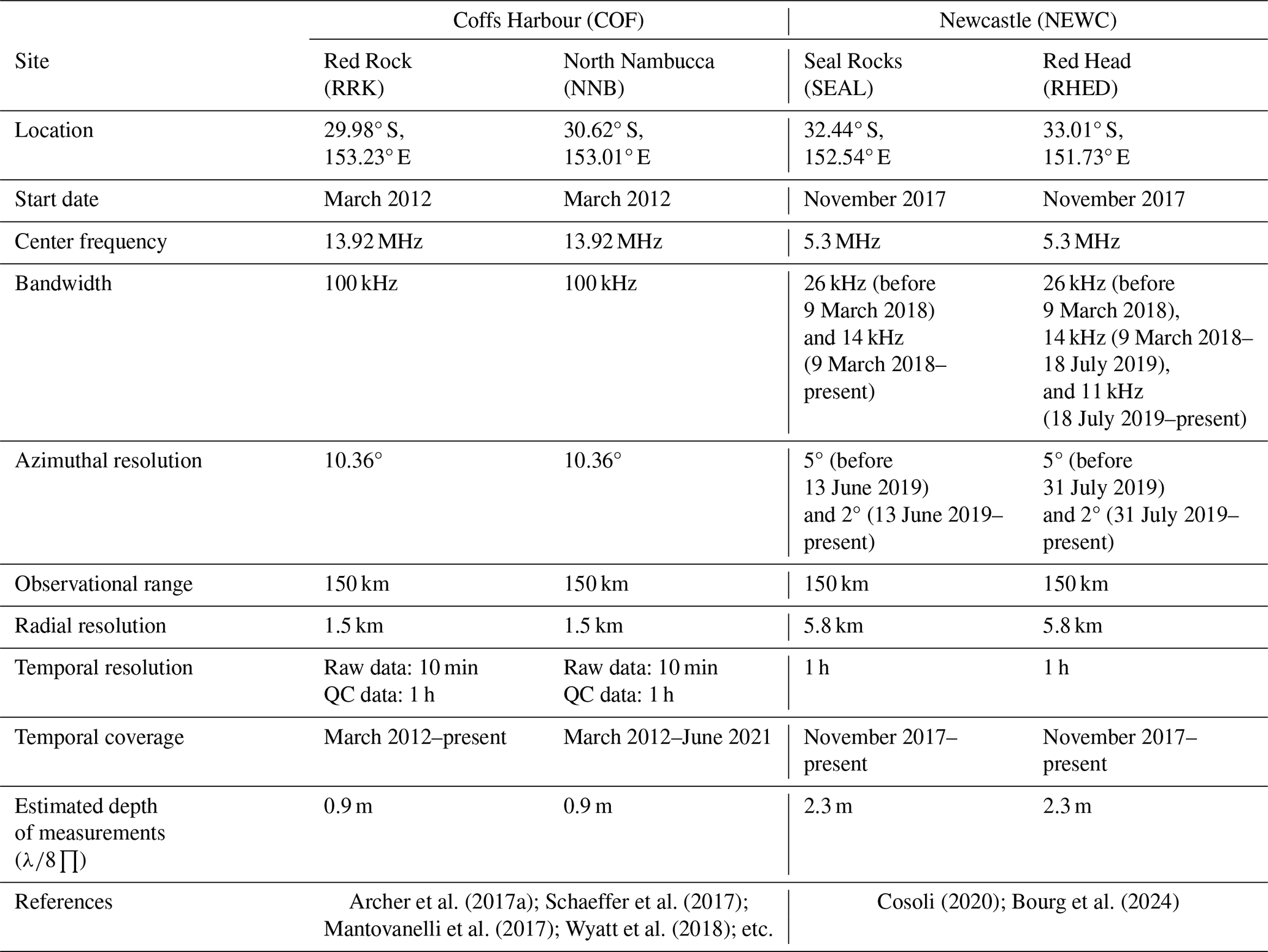
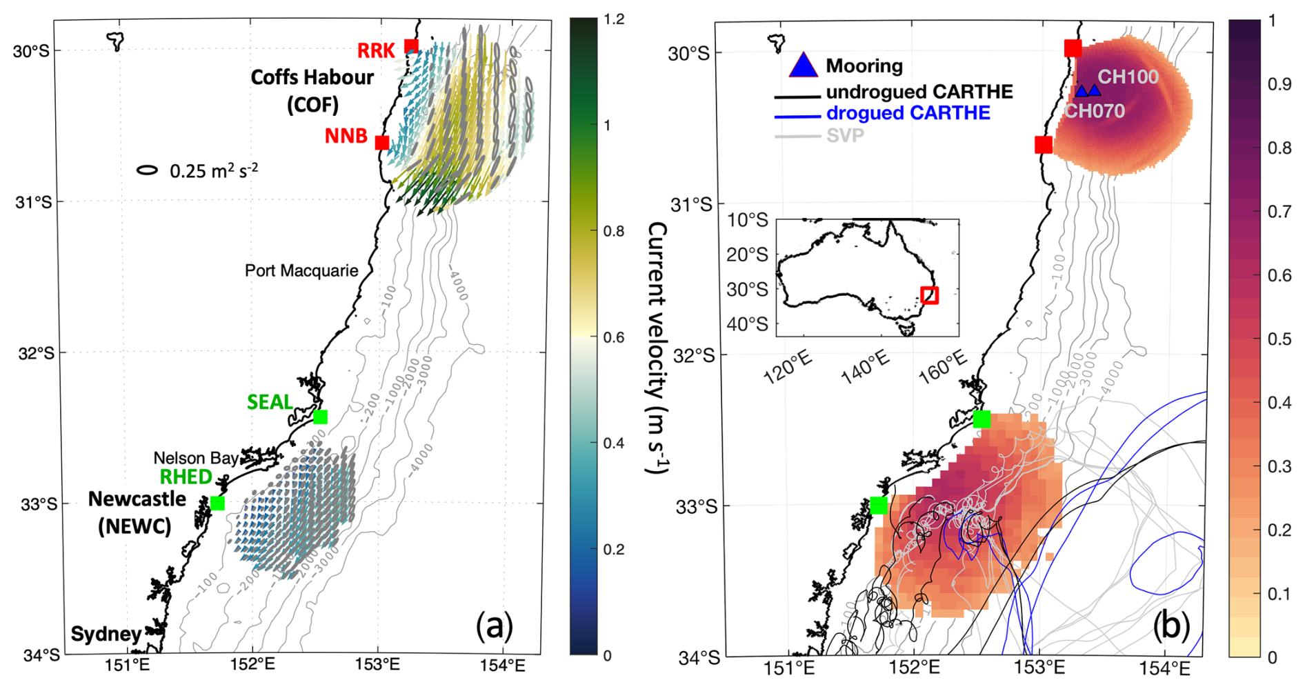
Figure 1 Maps showing the location of the radar sites along the eastern coast of Australia. (a) Temporal mean surface current vectors observed from the Coffs Harbour (COF; RRK + NNB) (2012–2021) and Newcastle (NEWC; SEAL + RHED) (2018–2023) radar sites. The ellipses denote the current velocity variance (plotted every two grid points). The color map depicts the mean velocity magnitude. (b) Maps of the mean spatial coverage (as a ratio from 0 to 1) were plotted separately for the two sites: COF (1 March 2012–1 January 2021) and NEWC (1 January 2018–1 January 2024). Data were averaged for a period of 8 years for COF and 4 years for NEWC. The metadata for each radar site can be found in Table 1. Also shown are the locations of the two subsurface current meter moorings at Coffs Harbour (CH070 and CH100) and the trajectories of the surface drifters used for validation of the NEWC system as described in Sect. 3.1.3.

3 Data and methods

3.1 Data quality control and availability

3.1.1 HF radar radial velocities

The radial data availability for each site from March 2012 to January 2024 is shown in Fig. 2. Since 2021, the Red Rocks (RRK) and North Nambucca (NNB) radars have experienced several hardware issues related to antennas, cables, hardware, and site computers. These issues affected radar operations, reducing the coverage of both radars. Consequently, both radar sites have been partially operational or nonoperational for the past 3 years. Radial data from all sites are freely available and accessible via the IMOS data server (https://thredds.aodn.org.au/thredds/catalog/IMOS/ACORN/catalog.html, last access: 1 October 2024). Inaccuracies in calculating the radial currents can arise from various factors, including radio wave interference from moving ships, misidentification of the Bragg peaks or the directional of arrival due to inadequate calibration of the antenna pattern, and additional uncertainties introduced during the vector-mapping process (Wyatt et al., 2018). In the real-time product, an IMOS standard quality control procedure is applied to remove the data outliers from the original radial data (FV00). A more comprehensive quality control (QC) procedure is then applied to the FV00 data to create a more accurate product, which is published to the AODN server after a delay of a few months and flagged as FV01 (as per Cosoli and Grcic, 2019). We refer the readers to Cosoli and Grcic (2019) for more information on the QC protocol. At the time of this study, the quality-controlled data are available for the COF region from 2012 to 2021; however, for the NEWC region, the quality-controlled data are available for the total current vectors, whereas they are only available for about 2 years, from May 2018 to October 2019, for the radials. Therefore, to acquire better data, further QC was applied to the FV00 radial data for the NEWC region. Here, we followed the method of Bourg et al. (2024), which is based on Cosoli and Grcic (2019), for removing outliers in the radial dataset. The outliers in the radial velocity were identified based on the absolute velocity exceeding 3 standard deviations across the entire time series as well as pixels with less than 30 % temporal coverage during a month. Then, the spatial and temporal gradients of velocity were examined to eliminate the data points with a probability of occurrence below 3 %. Finally, the gradient of absolute current speed for each grid cell over the whole dataset exceeding 3 standard deviations within a moving window of 30 points was considered a spike and removed. This procedure is iteratively repeated at every data grid cell to ensure quality across the entire dataset, leading to a cleaner and more robust dataset suitable for further analysis and interpretation.

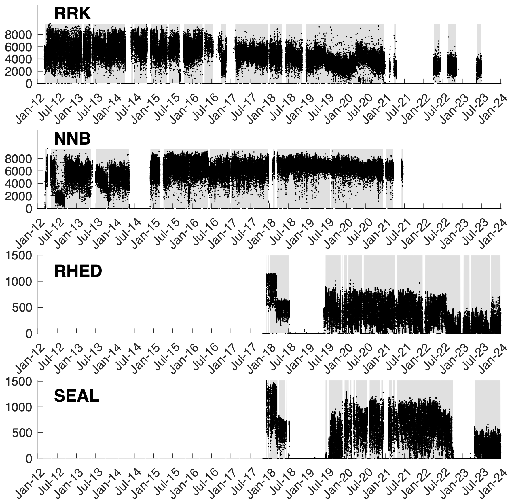
Figure 2 Temporal coverage of the data available at each radar site to date. Black points present the coverage of hourly radar data for each site. Gray shading represents the radar in operation, whereas the blank spaces show when the radar stopped working for more than 1 d.

3.1.2 Current meter mooring data

Two bottom-mounted acoustic Doppler current profilers (ADCPs) are located at the 70 m (CH070) and 100 m isobaths (CH100) across the shelf around 30° S (under COF radar coverage; Fig. 1a), in the middle of the COF domain providing current observations at high temporal resolution through the water column. Velocities were monitored with vertical bin sizes of 4 m and a sampling rate of 5 min. The data were quality-controlled using the IMOS Toolbox (https://github.com/aodn/imos-toolbox/releases, last access: 6 March 2025) before being averaged hourly, as described in Wood et al. (2016). The topmost bin of the velocities within the range from 9 to 11 m depth was used in this study. During the study period, mooring data were available for more than 90 % of the time (see Fig. A1 in the Appendix). For more information on the mooring data, readers are referred to Schaeffer et al. (2014) and Roughan et al. (2015).

3.1.3 Surface and subsurface drifters

Here, we use data from various drifter types, including the Consortium for Advanced Research on Transport of Hydrocarbon in the Environment (CARTHE) drifters, both with and without drogues, with drafts of 60 and 5 cm, respectively, and the Surface Velocity Program (SVP) drifters at 15 m depth. These drifters were released near the Newcastle (NEWC) HF radar during two separate campaigns conducted in November 2020 and October 2023. During the study period, 20 drifters deployed within the NEWC radar domain were collected, consisting of 7 surface CARTHE drifters and 13 subsurface SVP drifters (Lumpkin et al., 2017). The CARTHE drifters are donut-shaped, cost-effective, biodegradable instruments that aim to quantify the current transport and material dispersal (such as oil spills, pollutants, and marine debris) at the ocean surface. The flat design of the drifter is specifically tailored for tracking surface transport to a depth of 60 cm with the aid of a drogue. Their position is transmitted every 5 min through the Iridium satellite network. Along with the drogued CARTHE drifters, two CARTHE drifters without the drogues (drifting at about 5 cm) were also deployed to assess the effect of drifter slip velocity introduced by the wind and waves (Novelli et al., 2017).

The SVP drifter measures surface currents and other oceanographic parameters in the global oceans (Lumpkin et al., 2017). It is an important tool for studying ocean circulation patterns, understanding the role of currents in global climate, tracking pollutants, and monitoring marine ecosystems. During the years 2020 and 2023, 13 SVP drifters were deployed over the Hawkesbury Shelf (within the coverage of NEWC radar) to track the near-surface current and transport. Each SVP drifter was equipped with a holey-sock drogue centered at a depth of 15 m which helped to minimize the influence of wind and waves on the drifter's motion, allowing it to follow the ocean currents more accurately. The data were transmitted every hour. The availability of the drifter data is shown in Fig. A1.

In order to compare the drifter velocities with the radar-derived velocities, the drift velocities are computed using a finite-difference method along their trajectories at a regular time interval (1 h) to match the radar time resolution. The HF radar velocity in the closest cell to the drifter position is interpolated onto the drifter trajectories for comparison. The QC of the drifter to eliminate inaccurate GPS fixes was done as follows. Every drifter distance smaller than the GPS error (approximately 10 m) was removed from the dataset. Any drift speed exceeding 3 m s⁻¹, calculated using finite-differencing from the drifter data, was considered a spike and was filtered out. In addition, we applied a 6 h Gaussian filter window across the drifter speed to identify the trends following the initial spike removal. The discrepancies between the filtered and the raw data were assessed, allowing for the detection of abrupt changes by setting acceptable gradient thresholds. The data points were discarded if the drift speed surpassed the threshold higher than 1 standard deviation of the original drift speed.

3.1.4 Wind data

In this study, we use wind data from the high-resolution BARRA2 regional reanalysis dataset (Su, 2024), provided by the Bureau of Meteorology (BOM) in Australia. This choice is due to the limited availability of wind stations in our study region, which are mostly confined to coastal areas. The BARRA2 reanalysis data represent the second reanalysis version from the BOM, featuring an enhanced spatial resolution of 12 km and covering Australia and the surrounding regions. The data are available from 1979 to the present day and are provided on an hourly basis (Su, 2024).

3.2 Reconstruction of the surface current vectors

In principle, HF radar measures the surface currents using wavelengths that interact with surface gravity waves whose propagation is affected by currents at depths of 1 m to several meters (“Bragg scattering”). One radar can only measure the radial current velocity, which means the currents coming inward or outward of the radar along the radial beams. Therefore, obtaining a full picture of the ocean currents requires two or more radars with a common overlapping zone to complete a surface current map or the total currents.

While the IMOS radar team provides hourly current velocities interpolated using the LS approach, here we compare the IMOS data with the reconstructed data processed using the 2D variational (2dVar) interpolation approach (Yaremchuk and Sentchev, 2009), which is thought to produce a “best” velocity field v. The method is based on the maximum likelihood estimation of its Gaussian probability density function within a predefined oceanic domain Ω. The goal is to obtain the gridded velocity field v(x,y) at every time step t. With 2dVar, a cost function, J, is written in a quadratic form and consists of two arguments. The first term in Eq. (1) involves the minimization of the error between the unknown velocity v and the radar observations v_k. The error is scaled by the variance of the radar measurements at each point, σ²(v_k). The unknown velocities, v, are projected along each radial beam r_k with the bearing angle θ_r to derive a set of discrete data points at location $x_k,k=\mathrm{1},\mathrm{2},\mathrm{\dots }K$. In the second term, the algorithm enforces the pattern of the velocity field via regularizing the spatial derivatives of v, which are the divergence, $\mathrm{curl}v={\partial }_{x}v-{\partial }_{y}u$, and convergence of the velocity field, $\mathrm{div}v={\partial }_{x}u+{\partial }_{y}v$, within the domain bounded Ω. The Δ represents the Laplacian of divergence and vorticity of the velocity field. The smoothness parameters, W^d and W^c, in Eq. (1), are introduced at every grid point to facilitate the smoothness of the circulation pattern while limiting the generation of spurious small-scale variations in the reconstructed velocity field. Similarly, the last parameter, W^u, is introduced as an additional smoothness of the velocity field v, which was argued by Yaremchuk and Sentchev (2009) to enforce the coherence of the reconstructed velocity field. This approach maintains the extraction of important physical features in the flow field while reducing the number of artifacts from the interpolation. The weights W^u, W^d, and W^c have the meaning of inverse error variances of their respective fields, allowing control of their corresponding magnitudes in the reconstructed pattern (Yaremchuk and Sentchev, 2009). In this work, we performed a similar practice to that in Yaremchuk et al. (2016) for identifying the weight parameters of the 2dVar approach. The W^u was roughly estimated based on the following formula: W^u=0.05σ²l⁴, in which σ² represents the diagonal values of the noise covariance matrix from the radial data and l is the spatial resolution of the radial data. The equation represents the cutoff scale, which is approximately twice the spatial resolution of the radial data. After fixing the W^u value, we adjusted the value of W^c and W^d using the drifter data for NEWC and mooring data for COF radar until the optimal values were found. Surface velocities at the two sites that were constructed using the two methods are shown in Fig. 3. Compared with the surface current field generated by the LS approach (Fig. 3a, c), the spurious vectors lying in critical geometric dilution of precision (GDOP) regions are well reduced in the current field processed by the 2dVar method (Fig. 3b, d).

$$\begin{array}{}\text{(1)}& \begin{array}{rl}J& ={\displaystyle \frac{\mathrm{1}}{\mathrm{2}K}}\sum _{k=\mathrm{1}}^K{\mathit{\sigma }}^{-\mathrm{2}}\left(v_k\right)\left[\right({\widehat{P}}_{k}v)\cdot r_k-v_k{]}^{\mathrm{2}}\\ & +{\displaystyle \frac{\mathrm{1}}{\mathrm{2}A}}\underset{\mathrm{\Omega }}{\int }\left[W^d\right(\mathrm{\Delta }\mathrm{div}v{)}^{\mathrm{2}}+W^c(\mathrm{\Delta }\mathrm{curl}v{)}^{\mathrm{2}}\\ & +W^u\left(\mathrm{\Delta }v{)}^{\mathrm{2}}\right]\mathrm{d}\mathrm{\Omega }\end{array}\end{array}$$

Here, K is the number of radar observations, A is the area of the interpolation domain Ω, and ${\widehat{P}}_k$ is the projection of the reconstructed velocity v onto the radial beam at position x_k.

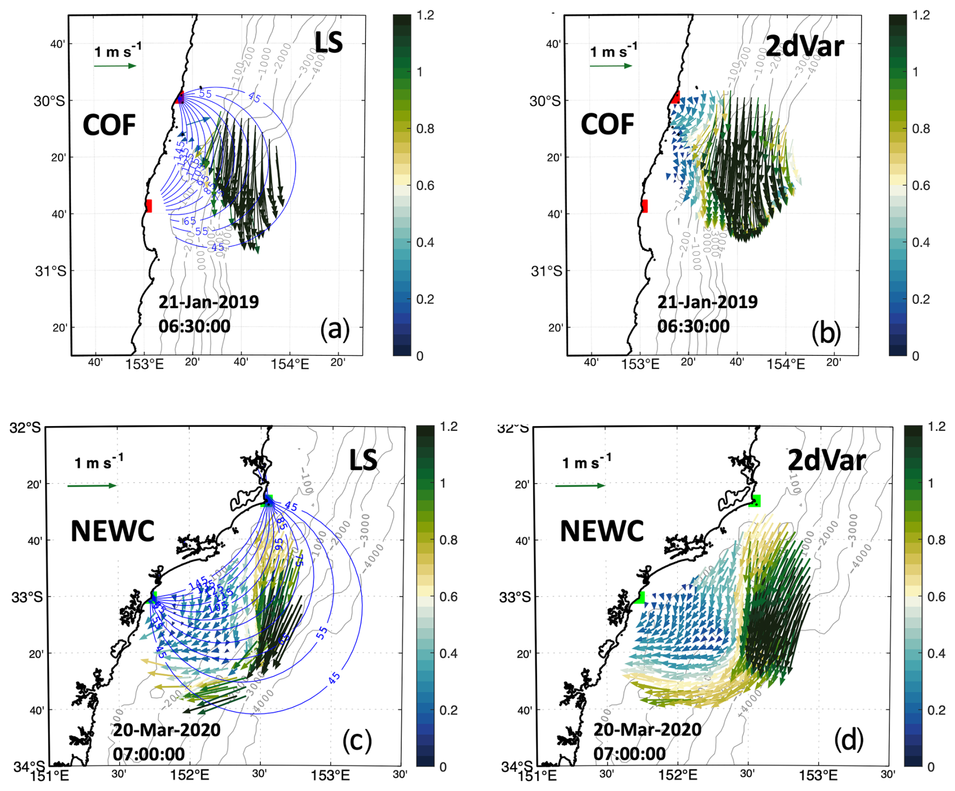
Figure 3 The snapshots of surface current fields reconstructed by the traditional unweighted least-squares (LS) fit (a, c) and by the 2dVar (b, d) methods for two radar sites. The vectors in COF are plotted every three grid points for visualization. The white band from the velocity color bar represents the speed threshold of 0.6 m s⁻¹. The blue contour shows the radial beams' intersecting angle (geometrical dilution of precision, GDOP). The current vectors are strictly between 45 and 145° of the GDOP.

3.3 Methods of analysis

3.3.1 Assessing the performance of the 2dVar approach

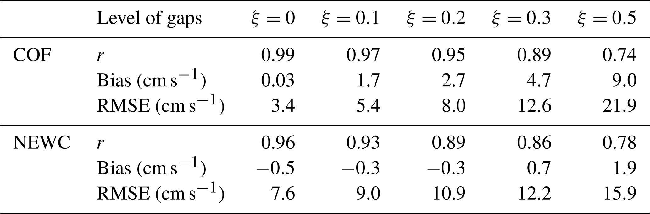
Using the 2dVar approach, we can fill the gaps in the reconstructed field, making it crucial to evaluate the performance of the method. For quantifying the accuracy of the 2dVar method, we employed cross-validation for comparison (e.g., Alvera-Azcárate et al., 2005). Some cross-validation points were chosen arbitrarily from 1160 radial current snapshots for NEWC radar and 1189 snapshots for COF radar with the best coverage. From each site, roughly 2 % of the total radial points were marked for validation, and these points were not used in the subsequent analysis. The remaining dataset was used to compute the total current vectors with the 2dVar method. These analyzed current vectors were then interpolated onto the locations corresponding to the cross-validation points, facilitating the evaluation of the accuracy of the analysis. Synthetic gaps were introduced into the original velocities covering 10 % (ξ=0.1) to 50 % (ξ=0.5) of the total grid. The total surface velocities after reprocessing with the 2dVar approach were projected onto the radial beam, $u_{\mathrm{r}}=u_{\mathrm{m}}\cos {\mathit{\theta }}_{\mathrm{r}}+v_{\mathrm{m}}\sin {\mathit{\theta }}_{\mathrm{r}}$. These points were then compared with the cross-validation points set aside. Details of the comparison between the reconstructed velocities with gaps and the original data are shown in Table 2.

In order to compare the radar-derived velocity with the in situ measurements from mooring and drifter data, we adopted some common statistical metrics used in previous studies (e.g., Liu et al., 2014). When comparing two scalar time series, the correlation coefficient (r) is a widely used statistical measure to quantify their agreement. This quantity is a statistical measure that quantifies the strength and direction of the linear relationship between two variables. Additionally, we used the mean bias error to qualify the misfit between the interpolated velocity X_m and the raw data $X_{\mathrm{m}}^{*}$.

$$\begin{array}{}\text{(2)}& \mathrm{Bias}=\langle |X_{\mathrm{m}}-X_{\mathrm{m}}^{*}|\rangle \end{array}$$

The angle brackets 〈…〉 represent the average over time. In practice, the root-mean-square error (RMSE) is also commonly used to measure the differences between predicted values and observed values, as it takes the mean error in the distance between two time series into account.

$$\begin{array}{}\text{(3)}& \mathrm{RMSE}=\sqrt{{\displaystyle \frac{\mathrm{1}}{N}}\sum _{t=\mathrm{1}}^N\left(X_{\mathrm{m}}\right(t)-X_{\mathrm{m}}(t){)}^{\mathrm{2}}}\end{array}$$

The last metric that we used for the comparison was the complex correlation between two time vectors (Kundu, 1976). The complex correlation coefficient (CC) provides a way to measure the full correlation between the two vectors, including both the amplitude correlation α and the phase angle displacement θ.

$$\begin{array}{}\text{(4)}& {\displaystyle }\mathit{\alpha }={\displaystyle \frac{\langle u_{\mathrm{o}}{u}_{\mathrm{m}}+v_{\mathrm{o}}{v}_{\mathrm{m}}\rangle +\langle u_{\mathrm{o}}{v}_{\mathrm{m}}+v_{\mathrm{o}}{u}_{\mathrm{m}}\rangle }{\sqrt{\langle u_{\mathrm{o}}^{\mathrm{2}}+v_{\mathrm{o}}^{\mathrm{2}}\rangle }\sqrt{\langle u_{\mathrm{m}}^{\mathrm{2}}+v_{\mathrm{m}}^{\mathrm{2}}\rangle }}}\text{(5)}& {\displaystyle }\mathit{\theta }=\arctan {\displaystyle \frac{\langle u_{\mathrm{o}}{v}_{\mathrm{m}}-v_{\mathrm{o}}{u}_{\mathrm{m}}\rangle }{\langle u_{\mathrm{o}}{u}_{\mathrm{m}}-v_{\mathrm{o}}{v}_{\mathrm{m}}\rangle }}\end{array}$$

Here, (u_o,v_o) and (u_m,v_m) represent the zonal and meridional components of the current from observations and HF radar, respectively.

3.3.2 EAC detection from HF radar

We used the COF radar data to detect the variability in the EAC following the algorithm of Archer et al. (2017a, b). This process is summarized as follows. To set up a coordinate system that moves along with the meandering jet stream instead of being fixed to geographic locations, we first need to identify the central core of the jet at each latitude. We do this by finding the location of the maximum southward velocity for each row of data going from south to north of the COF radar domain. Next, we calculate the general downstream direction that the jet core is traveling in at each of those central core points. Then, for each core point, we find all of the data points that lie along a line cutting perpendicularly across the jet core at that location. For each of these perpendicular points, we calculate its cross-stream distance away from the core. We also rotate its original east–west and north–south velocity components to make one component perpendicular to the core (the cross-stream component) and the other component along the core's downstream direction. Finally, we binned and re-gridded all of the data points using the cross-stream distance from the core as the cross-stream coordinate and using the latitude of the core point as the along-stream coordinate. This allows us to view the jet structure in a coordinate system that moves along with the meandering jet, rather than being tied to fixed geographic locations.

3.3.3 Time series analysis

Spectral analysis is employed to evaluate the intensity of diverse periodic signals within the data, ranging from tidal to interannual timescales. UTide tidal harmonic analysis was used to analyze the tidal currents (https://www.po.gso.uri.edu/~codiga/utide/utide.htm, last access: 1 October 2024). The UTide toolbox provides a robust algorithm for tidal harmonic analysis to extract tidal constituents from observed data, allowing one to handle data with gaps and outliers (Codiga, 2025). To evaluate the variability in low-frequency bands, we applied a fourth-order Butterworth low-pass filter to eliminate short-term fluctuations. In this study, the filtering was conducted with a 25 h cutoff frequency to remove tidal currents, a 30 d cutoff to filter out seasonal changes, and a 1-year cutoff to identify interannual variations in the radar-derived surface circulation. This allows us to isolate and study the different physical processes driving the ocean currents.

4 Results

4.1 Error analysis of the reconstructed velocities

4.1.1 Gap-filling performance using 2dVar

The RMSE discrepancy of the current fields reconstructed using the 2dVar method relative to the cross-validation points set aside is shown in Fig. 4. The accuracy of the resultant velocity field is related to the availability of the data, the accuracy of measurements, and the intersection of the radial beams (GDOP). It is shown that resultant velocity errors are within 5–7 cm s⁻¹ for the majority of the domain, while higher errors are found in the outer bound of the analysis domain (Fig. 4).Velocity errors were greater offshore, particularly near the SEAL radar site. This significant offshore discrepancy coincides with the highly energetic region of the EAC pathway (Fig. 3c, d). The surface currents in this region are also influenced by the energetic large-scale circulation, causing rapid changes in the circulation pattern (e.g., Fig. 4 in Malan et al., 2023). The large errors in the offshore region were likely due to multiple factors, including radar uncertainties, the location of the northern sites, and the complex dynamics of the region. The skill score for each of the synthetic-gap scenarios is shown in Table 2. For more than 20 % (ξ>0.2) of cutoff data in the domain, the reconstructed velocity map degrades quickly, with the mean error exceeding more than 50 % of the “true” velocity. For more than 30 % (ξ>0.3) of the data cutoff, the 2dVar struggles to reproduce the complex current fields, in which the finer-scale motions are lost, and the current field becomes smoother with an increasing number of gaps (not shown). Indeed, this result is quite similar to the experiment by Yaremchuk and Sentchev (2009) in Bodega Bay: the authors suggested that 80 %–90 % of observational points are required to acquire the most accurate velocity field.

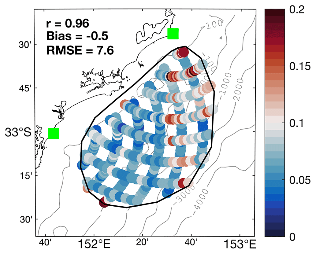
Figure 4 The RMSE discrepancy between the NEWC radial measurements and the 2dVar projection of the gap-filled velocity at the cross-validation points (in m s⁻¹). The black contour line delineates the boundary of the analysis domain, selected to encompass 80 % of the radar coverage.

Table 2 Comparison between the reconstructed data and the withheld data made at the cross-validation points. The radar velocities after reprocessing using the 2dVar approach were re-projected onto the radial beam. The ξ represents the level of gaps within the initial data, from 10 % (ξ=0.1) to 50 % (ξ=0.5).

4.1.2 Comparison with in situ and drifter velocity data

COF radar and mooring comparison

The COF radar data were compared with data from two current meter mooring stations (CH070 and CH100), while the data from NEWC were assessed with the drifter data (noting that there were no moorings at NEWC and no drifters at COF). The hourly radar-derived total velocities at COF from July 2012 to October 2020 were bi-linearly interpolated to the two mooring stations. Here, we compare two methods for reconstructing the total velocities (LS and 2dVar). The comparison between the radar-derived and topmost bin velocities of the moorings (approximately 9–11 m depth) was made using the common metrics, including complex correlation, phase difference, bias, and root-mean-square errors (Table 3), over about 8 years of data. We found that the HF radar velocities in the upstream region, which correspond to a depth of 0.9 m, showed a closer correlation with the in situ data collected at the CH100 site (∼0.89) compared with the CH070 site (∼0.73) and a larger cross-shore difference (∼0.20 m s⁻¹) (Table 3). Furthermore, the comparison of the v component (north–south, alongshore direction) from the mooring and the radar velocities from both methods (LS and 2dVar) also indicate a higher correlation than for the u component (east–west, cross-shelf direction) (Table 3). Applying a 25 h low-pass filter to both datasets, as was done in Wyatt et al. (2018), to remove the high-frequency variation, we found a slightly higher complex correlation α, ranging from 0.78 to 0.93, and the RMSE decreased to about 0.16 m s⁻¹. The θ values derived from both the LS and 2dVar methods were indeed similar, showing a more clockwise rotation of the subsurface mooring data compared with the surface radar-derived current vectors. A small discrepancy in angle of around 1° was found between the CH100 mooring location and the radar measurements, suggesting that the subsurface current vectors are nearly aligned with the surface radar vectors. The presence of the EAC likely unified the dynamics from the surface to deeper levels, which was shown to be present approximately 79 % of the time (Archer et al., 2017a). Despite a high correlation between the two data sources, a large discrepancy was particularly evident in the CH070 mooring data. The likely cause of this discrepancy can be attributed to the mooring's proximity to the coastline and the baseline between the two radar sites. The radar-derived velocity measurements at this location may have been compromised by interference from the antenna sidelobes or small-scale disturbances close to the coast, as suggested by Wyatt et al. (2018), leading to potential contamination or distortion of the u component.

NEWC radar and drifter comparison

Drifters were within the domain of the NEWC radar coverage for a total of 44 d (Fig. A1). In general, the examination of the NEWC radar-derived total velocities with the drifter velocities for two deployments (from 10 to 13 November 2020 and from 10 to 15 October 2023) showed that the radar-derived velocities compared well with drifter velocities. The comparison between the radar and drifter velocities was made within the time frame that the drifters were present inside the radar domain (Table 4). While the November 2020 deployment produced around 3 d of drifter data, the coastal drifter group provided significantly less, with only about 1 d of data (Fig. 5b, c). In October 2023, the drifters were released in the middle of the radar domain (not shown). In contrast, drifters (composed of the undrogued CARTHE and the SVP drifters) were deployed in two separate locations in November 2020: one group was close to the shore, whereas the other group was deployed about 20 km offshore. The time evolution of the drifter and the radar-derived current vectors indicated a reversal of CARTHE drifter vectors with respect to radar-derived current vectors (Fig. 5b, d), while a better agreement was found between the SVP drifters and the radar (Fig. 5c, e). In the first 12 h after release, the wind blew quite consistently in the west-southwest direction (Fig. 5a), while the current directions were north to northwest (Fig. 5b–d). The lack of a drogue in the CARTHE drifter increases its sensitivity to Stokes drift (Novelli et al., 2017), causing the offshore CARTHE to closely follow the wind direction (Fig. 5d). This behavior contrasts with that of the SVP drifter and radar-derived current vectors (Fig. 5e). Although it shows a high correlation (α ∼ 0.81–0.86; Table 4), the slip velocity caused by the wind may account for the observed discrepancy of approximately 10 cm s⁻¹ in the downwind direction between the radar and the undrogued CARTHE drifters, i.e., from 00:00 to 06:00 UTC on 10 November 2020 and from 06:00 to 18:00 UTC on 11 November 2020 (Fig. 5b, d).

The 2dVar method performed slightly better than the traditional LS method with respect to all common statistics as well as increasing the data coverage, with a complex correlation α of about 0.77 to 0.90 and an RMSE of about 7–9 cm s⁻¹ (Table 4). A positive bias speed was found across nearly all types of drifters, except for the nearshore group in the 2020 deployment, ranging from 2 to 4 cm s⁻¹ for the SVP drifters and from 7 to 8 cm s⁻¹ for the CARTHE drifters. This can be explained by the approximate 2 cm s⁻¹ underestimation of the radar-derived velocities due to the smoothing effects of spatial (∼13 km) and temporal (∼1 h) averaging, similar to the study of Rypina et al. (2014). The θ value, representing the rotation of the drifter and the radar vectors, showed a larger spreading angle of up to 5° between both methods (Table 4). This was more apparent for the drifter at the edge of the radar domain, such as for the nearshore-group drifter in 2020, and was possibly caused by the constraints of the 2dVar algorithm with respect to maintaining the consistency of the velocity map (Yaremchuk et al., 2016). Other than that, a more variable θ value was found across all of the drifters (Table 4), possibly due to a strong vertical shear between the radar velocity and different types of drifter velocity. The included radar velocities extrapolated by the 2dVar method slightly reduced the correlation α from 0.85 to 0.77; however, the RMSE increased to about 9–12 in the 2020 experiment and 12–15 cm s⁻¹ in the 2023 experiment. Rather than the increase in the noise level in the radar measurements, the increase in uncertainties in the 2023 experiment was possibly primarily due to the extra interpolation necessitated by the large decrease in the coverage of radial measurements, which was often lower than 80 % (ξ=0.22) and occasionally dropped to only about 10 % of the radar domain (not shown).

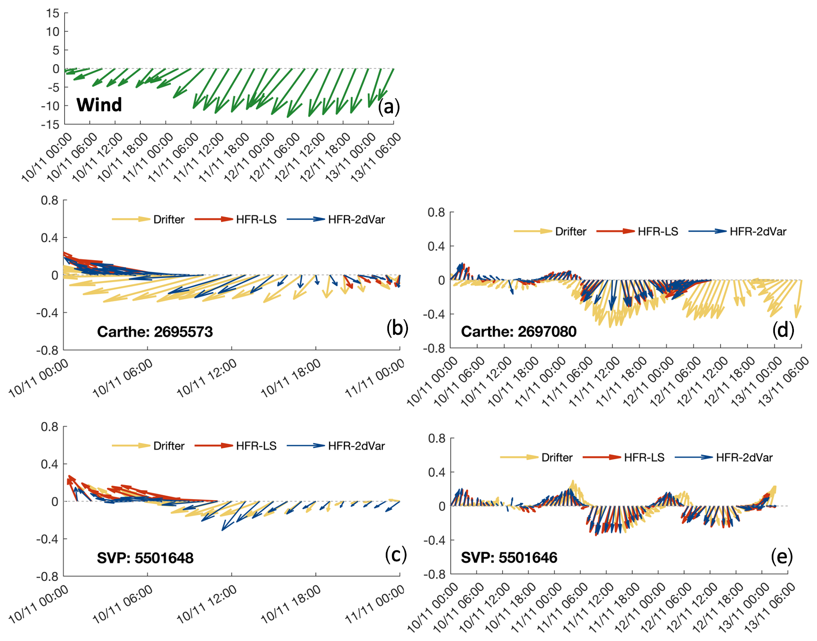
Figure 5 An example of wind averaged over the NEWC radar region, for the drifter deployment from 10 to 13 November 2020, is presented (a). The velocities of drifters deployed close to the shore (b, c) and in the middle region (d, e) are shown, superimposed by the radar-derived velocities extracted along the drifter trajectories using two reprocessing methods. The unit is meters per second (m s⁻¹).

Table 3 Comparison of the hourly radar-derived velocities processed with the two different gap-filling methods (LS or 2dVar) with moored velocity datasets at COF. The moorings are located above the 70 m isobath (CH070) and 100 m isobath (CH100) with currents measured at a depth of ∼9 m below the surface and data used from July 2012 to October 2020. The gap-filling method (LS or 2dVar) is indicated. N is the number of data points used in the comparison; α is the complex correlation; θ is the phase difference in degrees; and the bias and root-mean-square error (RMSE) values (m s⁻¹) in u, v, and total are shown.

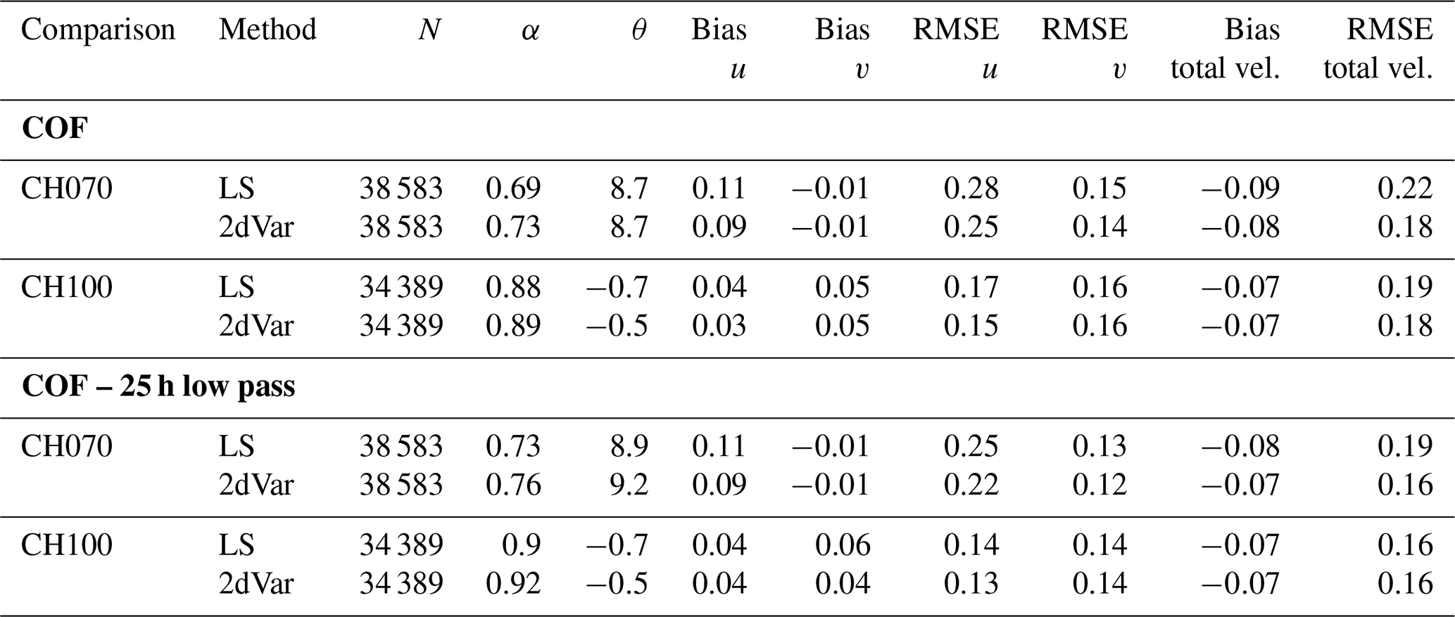
Note that for a phase difference θ>0, in situ vectors rotate counterclockwise to the HF radar vectors; for a Bias<0, in situ data are smaller than the HF radar measurement and vice versa.

Table 4 Comparison of the hourly radar-derived velocities processed with different methods with the drifter datasets from NEWC. The drifter velocities were taken from two different types of surface drifters: CARTHE with a drogue depth of 60 cm and SVP with a drogue depth of ∼ 15 m. An additional comparison with the undrogued CARTHE drifters (representing the top few centimeters of the water column) is shown. The lack of the drogue makes the drifter more susceptible to surface wind. The numbers in parentheses represent comparisons made with an extrapolation using the 2dVar gap-filling method. The bias and RMSE are in units of meters per second (m s⁻¹). The average level of gap, ξ, is shown for each drifter deployment.

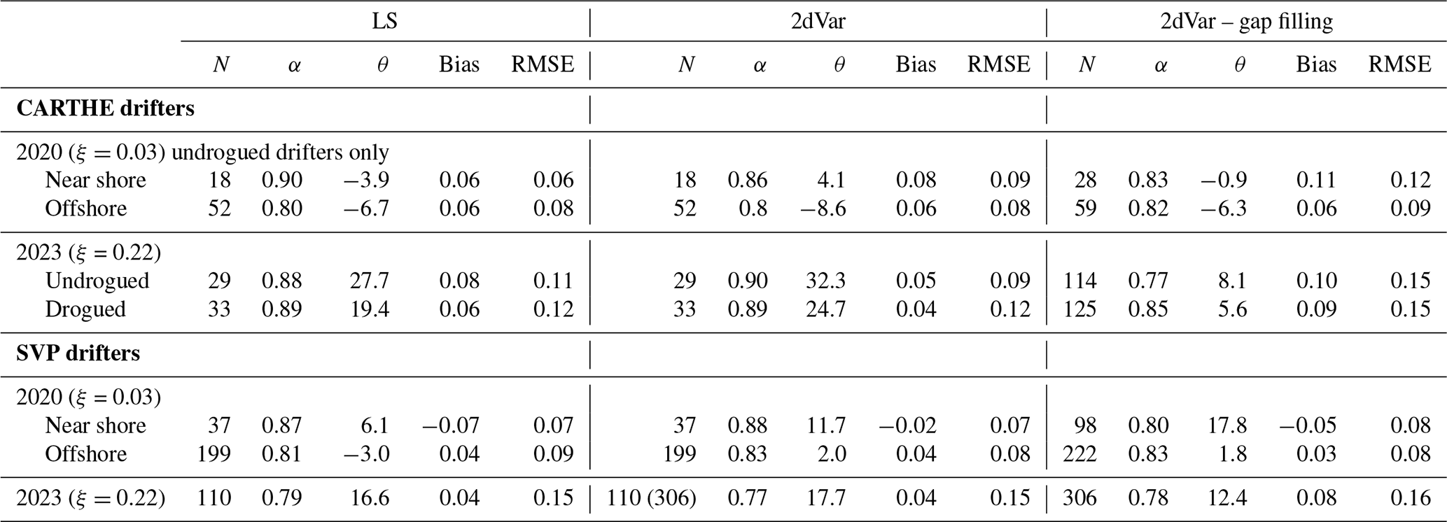
Note that for a phase difference θ>0, current meter velocities rotate counterclockwise to the HF radar vectors; for a Bias<0, current meter velocities are smaller than the HF radar measurements and vice versa.

4.2 Spectral analysis of the EAC jet and shelf velocities

For a better understanding of the surface circulation variability, we performed a spectral analysis of the surface current velocity time series. Three sets of approximately 2-year velocity time series were extracted at two locations (one co-located with the CH100 mooring point in the COF region near the EAC core and the other located offshore of the NEWC region) (33.00° S, 152.53° E). The core velocity of the EAC is identified using the jet-following method, as in Archer et al. (2017b). The length of the analysis period is selected to maximize the overlapping operating period between the two radar systems while also maintaining an acceptable data length. Figure 6 represents the velocity variance spectrum computed from the extracted surface velocity in the COF and NEWC regions.

Spectral analysis of the two datasets indicates similar patterns. The slope fittings across all scale bands for the core velocity, CH100, COF, and NEWC are approximately −1.54, −1.60, −1.59, and −1.55, respectively, which are quite similar to the energy-cascading theory of the Taylor scaling ($-\mathrm{5}/\mathrm{3}=-\mathrm{1.67}$) in the Kolmogorov spectrum (Fig. 6). Spectra derived from the mooring and radar velocity data (Fig. 6b) demonstrate that the EAC jet varies over multiple timescales – from short tidal and weather periods to durations of months. Weather and small-scale disturbances can trigger the EAC jet variability at a synoptic timescale, which is a relatively short period of 3–20 d. It has been shown that the EAC exhibits intrinsic variability driven by wind stress variations. Regional wind stress variations with periods shorter than 56 d enhance the EAC extension mean transport (Bull et al., 2017). Longer-period variations also occur, with cycles of around 65–100 and 25–40 d (Fig. 6a). These variability timescales are linked to the intrinsic variability in the jet meandering on and off the continental shelf region, as documented in previous studies (e.g., Bowen et al., 2005; Sloyan et al., 2016; Archer et al., 2017a).

As the EAC is an important driver of circulation in the region, both upstream and downstream shelf regions exhibit similar timescales, although the low-frequency peaks are shifted due to the modulation of the shallow waters. Distinct spectral peaks are observed at tidal frequencies, monthly to bi-monthly (25–60 d) and within the range of mesoscale bands from 70 to 200 d (Kerry and Roughan, 2020). The intra-annual peaks (>100 d) in both upstream and downstream regions are more pronounced in the shelf velocities (Fig. 6b, c) compared with the EAC jet velocities (Fig. 6a) and also present in the spectra derived from mooring data. The spectrum from the COF radar data indicates that the energy within the bands from 25 to 40 d is comparable to that of the intra-annual bands and is roughly 0.5 orders of magnitude greater than that in the downstream region at similar frequencies (Fig. 6b). The energy within these bands is broad and extends toward the synoptic bands, indicating that the variability in shelf waters at these timescales is likely driven by the energetic meandering of the EAC and its characteristic periods of eddy shedding (Archer et al., 2017a; Ribbat et al., 2020).

On the other hand, discrepancies between the mooring and the radar-derived velocities can be found in the synoptic range (3–20 d), where the radar data exhibit higher variability, approximately 0.5 orders of magnitude greater than the mooring data (Fig. 6b). This difference likely arises from the different depths of the observations: 10 m for CH100 mooring compared with 0.9 m for COF radar. Upon closer inspection, small and broad synoptic peaks (3–20 d) are evident in both the EAC variability and the shelf velocities, although they remain weak downstream. However, these synoptic signals are not as pronounced in the mooring velocity measurements. The enhanced synoptic variability in the radar data is likely due to local motions related to weather fluctuations and frontal eddies (Schaeffer et al., 2017). These smaller-scale instabilities are typically located inshore of the jet, resulting in a stronger energy level in the spectrum than the jet offshore.

In the high-frequency ranges, all spectra indicate the same level of energy with the semidiurnal peaks (M2 and S2) being smaller and narrower than the diurnal peaks (K1 and O1) (Fig. 6b, c). The semidiurnal peaks in the NEWC data are even smaller than in the COF region, suggesting the dominance of a diurnal tidal regime in this region (Fig. 6c). Within the diurnal bands, the near-inertial frequencies closely match the diurnal frequencies, especially at COF (23.6 h for COF and 22.0 h for NEWC). As a result, the diurnal energy can be affected by the inertial motions. The strong diurnal variability can also result from near-inertial period motions (at around 30° N and 30° S) close to the diurnal forcing driven by tides and land–sea breezes. This can also be influenced by the background vorticity or potentially amplified at the critical latitudes (Archer et al., 2017a).

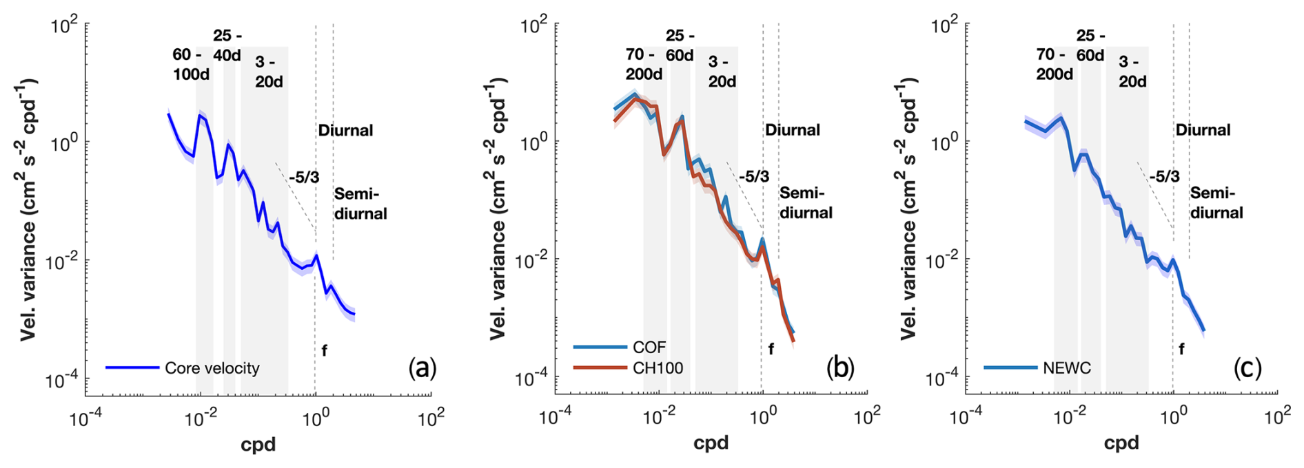
Figure 6 Spectral analysis of the hourly radar-derived current speeds during a 2-year period (1 January 2019 to 1 January 2021) of the EAC core velocity (a) and of a point at the CH100 mooring location (30.26° S, 153.39° E) in COF (b) and a point above the 200 m isobath off NEWC (33.00° S, 152.53° E) during the period from 1 September 2019 to 1 September 2021 (c). Inertial frequencies (f) of 23.6 and 22.1 h in COF and NEWC, respectively, are shown in the spectrum. The slope $-\mathrm{5}/\mathrm{3}$ represents the theory of energy cascading in the inertial range of the Kolmogorov turbulent spectrum. The 95 % uncertainties are shown by the blue and red shading.

4.3 Tidal variability

Hourly radar measurements can be used to examine tidal dynamics in the region. To further examine the capability of observing tidal currents from HF radar, the major tidal constituents (M2, S2, K1, and O1) are estimated from hourly COF radar and mooring data using the UTide toolbox (Codiga, 2025) during the year 2019, suggesting a general agreement with respect to the shape and size of the tidal ellipses (Fig. A3).

The tidal harmonic analysis is shown in Fig. 7. The spatial distribution of total velocity variance shows that tidal motions contribute a minor portion to surface current variability in both regions. This contribution is approximately 5 % in the offshore region of COF but is higher towards the shallow shelf in NEWC, with a contribution of around 15 %. The average tidal contribution to total surface variability is generally less than 10 %, as the shelf circulation is predominantly influenced by the EAC.

Regarding tidal magnitude, the upstream region's tidal regime is primarily governed by semidiurnal tides. The M2 tidal magnitude (about 0.04 m s⁻¹) is twice as large as the diurnal tides (K1 and O1, approximately 0.02 m s⁻¹), as shown in Fig. 7. Closer to the shore downstream, the diurnal tidal regime becomes more significant. The K1 tidal magnitude, derived from NEWC radar, is the most substantial among the four tidal constituents, with a value of roughly 0.06 m s⁻¹ (Fig. 7). Nonetheless, the overall tidal magnitude remains small, varying from 0.02 m s⁻¹ offshore to about 0.06 m s⁻¹ in shallow waters.

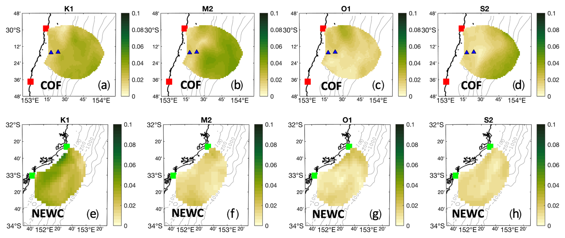
Figure 7 Magnitude of the major tidal ellipses derived from a 1-year period (from 1 January 2019 to 1 January 2020) of radar current velocities for four main tidal constituents: diurnal (K1 and O1) and semidiurnal (M2 and S2) tides.

4.4 Seasonal and spatial variability in the surface currents

Next, we examine how the shelf circulation responds to the seasonal cycle of the EAC. We begin our analysis by examining the current velocities upstream of the separation zone using COF radar data. To calculate the monthly mean surface currents at COF, we use an average of the data grid cells that cover a period of more than 5 years. Throughout the year, the monthly mean current vectors consistently point poleward, with notable variation in their magnitude (Fig. 8). The radar-derived current patterns indicate that the EAC strongly modulates the local circulation, with mean current velocities gradually increasing offshore. The oceanic jet follows the isobaths and is influenced by the underlying topography. This is shown by the jet boundary, visually identified by the −0.6 m s⁻¹ velocity line, which rarely extends inshore beyond the 200 m isobath (Fig. 8). The core of the EAC, indicated by the highest mean velocities, flows in a region above the 1500 and 2000 m depth contours, which is consistent with previous findings by Archer et al. (2018). The jet-funneling effect, as detailed by Oke and Middleton (2000), is apparent in the southern domain. The term refers to a narrowing and an increase in the jet intensity through the narrow shelf. It was shown by the higher mean velocity and the current variance ellipses that orient towards the shore in the south of the domain (Fig. 8). Corresponding to the variability in the EAC, the strongest monthly averaged currents are observed during the austral summer, whereas these currents are weaker during the austral winter. In November and February, the EAC strengthens, and the radar-derived currents show that the highest velocities reach approximately 1.4 m s⁻¹ at the core of the EAC with high variation (approximately 0.3 m s⁻¹). However, during June, the EAC footprint is minimal, resulting in much weaker mean currents (Fig. 8).

Compared with the upstream region, the NEWC data are more limited, as the dataset only spans 4 years. January and December are the 2 months with the lowest data availability of about 2 years (Fig. A2). Despite this limitation, it is evident that the surface currents quickly lose momentum and decrease in magnitude at the separation region (Fig. 9) compared with the upstream region. This results from the fact that the EAC typically separates around this latitude, bifurcating into the eastern and southward extensions (Oke et al., 2019). Past the separation point, the southward extension of the EAC broadens and shallows, becoming more barotropic and decreasing its poleward transport (Kerry and Roughan, 2020). Around 32.5° S, the EAC signature from the mean velocity field appears to turn eastward and veer away from the continental shelf, likely experiencing an “inertial overshooting” effect from the westward-bending shelf (Oke and Middleton, 2000). Based on the radar-derived data, we found that the current evolution downstream does not entirely follow the seasonality of the currents upstream and demonstrates a more complex variability. This can be shown by the maxima of current velocity flowing along the shelf that occurs during February (∼ 0.6 m s⁻¹), whereas the strong current patterns persist and shift more offshore during March and April (Fig. 9). On the other hand, the downstream average current speed decreases during November and December off NEWC (but increases at COF; Fig. 8). Given the differences between the monthly variability upstream and downstream, one may suggest that it is due to the difference in the average period of both data sources. However, it has been shown that the circulation downstream of the EAC is rather complex and closely related to the mesoscale circulation driven by the EAC eddy-shedding timescales (Kerry and Roughan, 2020).

The intra-annual change in the surface circulation was examined using the monthly averaged velocity (Fig. 10). The daily radar-derived velocities in both regions were averaged over the whole domain to assess the mean and standard deviation for each month of the year. Velocities were rotated by 18 and 30° for COF and NEWC data, respectively, to derive the alongshore and cross-shore components, based on the predominant orientation of current variance ellipses (Figs. 8 and 9). The monthly averaged velocities indicate a poleward mean transport (negative alongshore velocities) at both sites that is consistent throughout the year (Fig. 10). The COF radar-derived velocities show that the annual cycle of poleward transport exhibits peaks (at around 0.80 m s⁻¹) in the early and late summer (November and February) and that the lowest poleward transport value (about 0.25 m s⁻¹) occurs in the winter months (June and July). The range of monthly variation, approximately 0.4 m s⁻¹, is larger than the standard deviation and exceeds the average wintertime velocity (Fig. 10b). The monthly patterns reveal slight increases in alongshore velocity during autumn (April) and spring (August to October).

Off NEWC, there is a strong annual cycle in the alongshore direction, although the velocities are weaker, ranging from 0.4 to 0.1 m s⁻¹ from summer to winter, respectively (Fig. 10b). On the other hand, the cross-shore component in both regions does not show a seasonal pattern but, rather, varies significantly throughout the year. The increase in cross-shelf exchange upstream is driven by the meandering of the surface-intensified jet on and off the shelf (Malan et al., 2022); thus, the variability occurs in both magnitude and sign. The mean cross-shelf velocity downstream remains similar; however, the standard deviation is half as much as that found upstream (Fig. 10a).

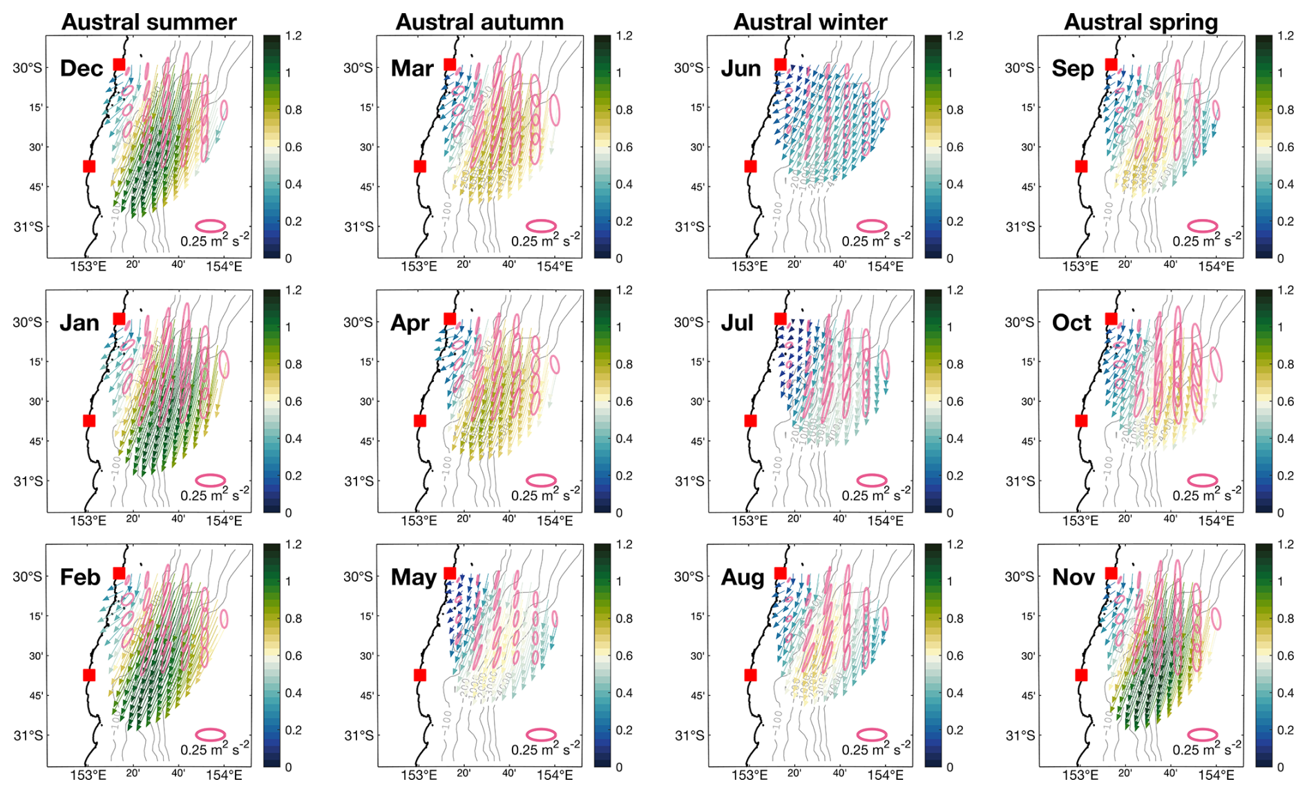
Figure 8 Maps showing the monthly mean radar-derived current vectors at Coffs Harbour (upstream) using hourly data from the COF radar from March 2012 to January 2021. The monthly mean current maps are organized by season in each column. The velocity is given in meters per second (m s⁻¹). The current velocity variances are illustrated by plotting ellipses at six grid point intervals for visualization. The bathymetry contours are plotted at the 100, 200, 1000, 2000, 3000, and 4000 m levels.

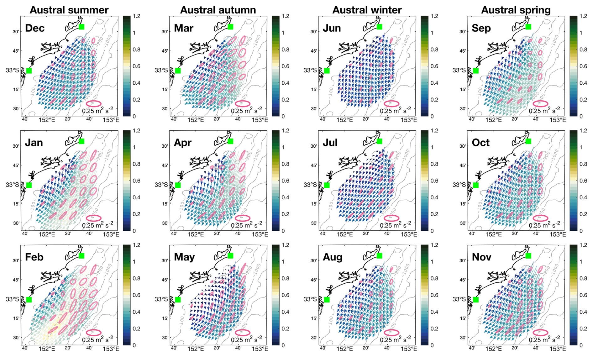
Figure 9 Maps showing the monthly mean radar-derived current vectors off Newcastle using hourly data from the NEWC radar from November 2017 to February 2024. The monthly mean current maps are organized by season in each column. The velocity is given in meters per second (m s⁻¹). The current velocity variances are illustrated by plotting ellipses at two grid point intervals for visualization. The bathymetry contours are plotted at the 100, 200, 1000, 2000, 3000, and 4000 m levels.

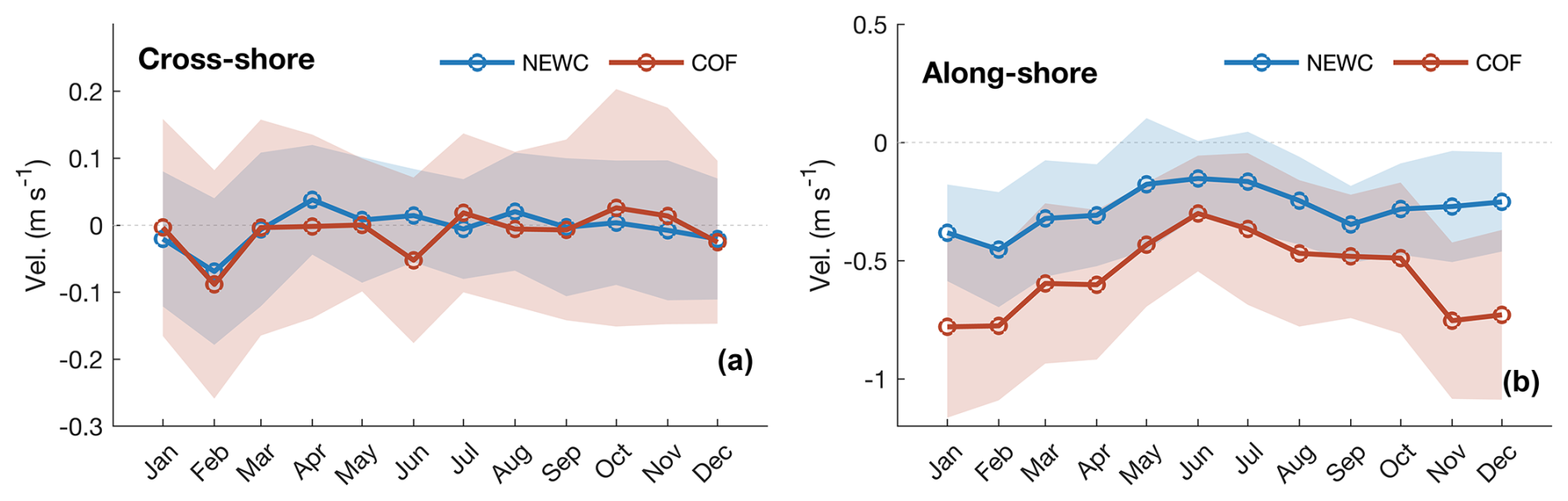
Figure 10 Domain-averaged monthly radar-derived (a) cross-shore and (b) alongshore velocity plotted as a function of the month for COF and NEWC, respectively. The velocity vectors are rotated 18° clockwise for COF and 30° clockwise for NEWC to obtain the cross-shore and alongshore velocities accordingly. A positive value of the alongshore (cross-shore) velocity represents the northward (offshore) transport and vice versa. The shaded area denotes the standard deviation of domain-averaged velocities.

4.5 Seasonal and intra-annual variability in the EAC jet

The EAC proper demonstrates a pronounced seasonal cycle in temperature and velocity, a subject that has been explored in previous studies (e.g., Godfrey et al., 1980; Ridgway and Godfrey, 1997). Moreover, Archer et al. (2017a), using the jet-following method and COF radar data from 2012 to 2016, revealed that the EAC magnitude and its associated variance follow a seasonal pattern, peaking during summer. Here, we extend the analysis and summarize the key findings of the EAC characteristics using a longer dataset of around 8 years. As the EAC consistently oscillates on and off the continental shelf, with the offshore extension of the jet core up to 90 km from the coastline (Archer et al., 2017a) and, thus, disappearing from the radar footprint, the jet-following method, used in Fig. 11, enables the detection and characterization of EAC signals within its coherent structure. The jet exhibits an asymmetric behavior. Indeed, on its eastern side, it can freely meander and shift laterally over the open ocean, but its western flank is constrained by the presence of the continental landmass, limiting how far it can veer in that direction. What can be seen from this analysis is the monthly fluctuation in the EAC's intensity, peaking during midsummer (January; mean speed of approximately 1.5 m s⁻¹) and reaching its lowest point in winter (June; mean speed of approximately 0.9 m s⁻¹), with an annual difference (0.6 m s⁻¹) of around 40 % of the mean velocity (1.35 m s⁻¹) (Fig. 11). The jet-following method identifies a stronger EAC in late winter (July and August; with velocities of around 1.2 ± 0.2 m s⁻¹), although this contrasts with the weaker jet speeds of approximately 0.6 ± 0.2 m s⁻¹ observed in the monthly mean surface velocity map (Fig. 8). From May to August, the EAC jet exhibits large variability during winter, and this variability is more pronounced on the right flank than on the left, as the jet is narrower in winter (Fig. 11). As shown by the extension of the jet cross-structure, the jet can be widened during the period from December to February when the EAC is strongest (approximately 60 km), but the widening jet can also be found during June when the EAC is weakest. The variability in the jet width over the year exhibits a range of variation of around 10 km (Fig. 11).

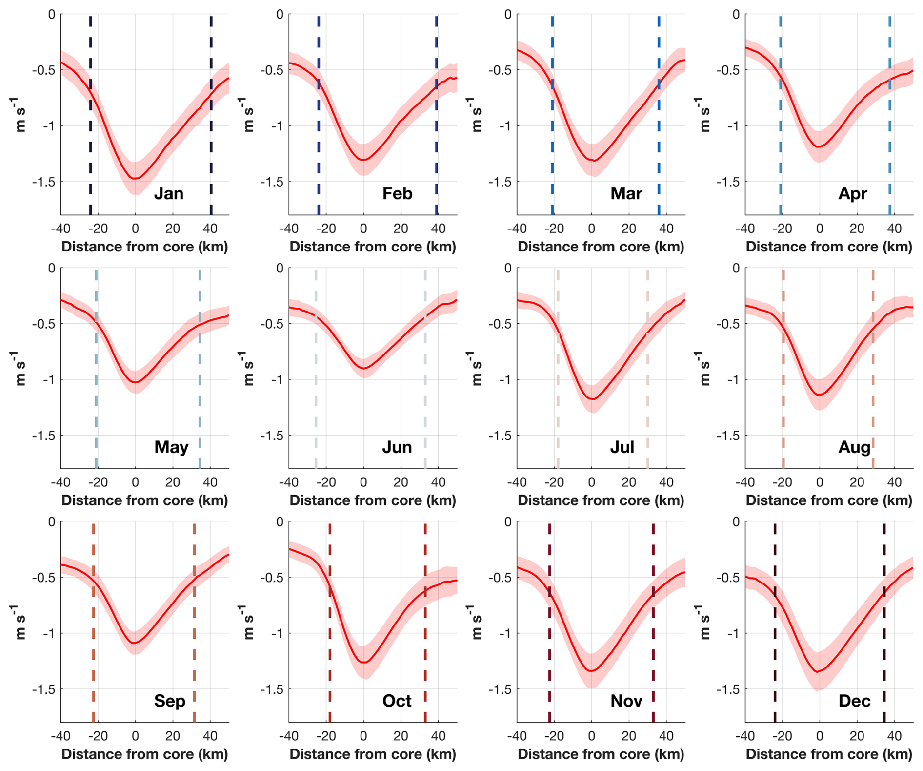
Figure 11 Annual cycle of the EAC cross-structure identified using the jet-following method (Archer et al., 2017b) based on 8 years of Coffs Harbour (COF) data. A positive value indicates the southward movement of the jet. The cross-structure of the jet is averaged from 30.2 to 30.6° S. Red lines represent the mean poleward magnitude of the EAC across the jet. Shaded areas represent 1 standard deviation from the mean speed. Dashed lines mark the boundary of the EAC, defined as points with a 50 % reduction compared with the core velocity.

4.6 Interannual variability in the EAC as observed from the radar

The poleward transport anomalies of the EAC in the COF radar data also show strong interannual variability (Fig. 12c). The lowest transport occurred in late-June to November 2017, which is consistent with the observations of a large and long-lived cyclonic eddy generated during that time of the year (Roughan et al., 2017). The data also suggest a shift in the jet core position from late 2019 to mid-2020, as demonstrated by the maximum core velocity moving toward the 1000 m isobath, which led to a significant increase in the average shelf velocity (Fig. 12a). This shift was followed by a reversal to its average position by late 2020 (Fig. 12c). A similar event appears to have occurred in January 2015, marked by an increase in along-shelf velocity, as shown by mooring and radar data (Fig. 12c).

The velocity time series from the CH100 mooring and data extracted at the same location from COF radar are shown for comparison (Fig. 12c). The estimated interannual variation contributions to total alongshore velocity variances from COF and CH100 mooring observations were nearly identical, about 12 % and 10 %, using the radar-derived velocity and CH100 mooring data, respectively. Results from the COF alongshore velocity and the mooring velocities show a significant change in the timescale of more than 4 years, which is shown by two phases of the increasing and decreasing of the EAC core velocity (Fig. 12a). The EAC signals observed from the CH100 mooring location became stronger during January 2015, with the velocity anomaly exceeding 0.25 m s⁻¹ (0.3 m s⁻¹ from the CH100 mooring), whereas it weakened during the following summer (Fig. 12c). From 2017 onward, another pattern of strengthening and weakening of the EAC is consistent with the mooring observations. Another weak period of the EAC can be seen from the CH100 mooring, occurring from January 2020 and lasting until January 2023; however, unfortunately, COF radar data were not available for this whole period (Fig. 12c). Despite the differences between the two datasets, the consensus on the EAC patterns reinforces our method's reliability for processing radar measurements over interannual and longer timescales.

Downstream of the EAC, the interannual variability accounts for about 14 % of total variability for both alongshore and cross-shore velocity (not shown). Although the mean alongshore velocity downstream is approximately half of the upstream mean velocity, it surprisingly exhibits interannual variations of up to 0.4 m⁻¹, comparable to the more energetic environment upstream (Fig. 12a). The interannual variability in the NEWC alongshore velocity exhibits a complex pattern. Maximum poleward transport through the NEWC region occurred from January to May 2022, coinciding with the weakened mean EAC intensity indicated by CH100 mooring data. Conversely, the southward velocity anomaly decreased in 2023 as the EAC intensified (Fig. 12c).

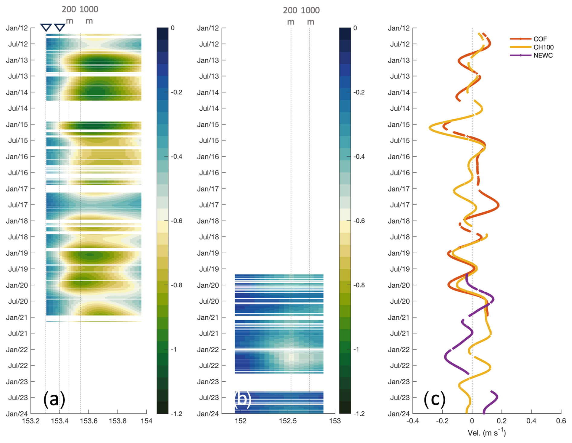
Figure 12 Hovmöller plot showing the interannual and intra-annual variability in the 1-year low-pass-filtered radar-derived alongshore velocity (in m s⁻¹) at (a) Coffs Harbour (COF) along a line normal to the shore from 30.26° S and at (b) Newcastle (NEWC) along a line normal to the shore from 33.06° S. The velocity vectors are rotated 18° clockwise for COF and 30° clockwise for NEWC to obtain the alongshore velocities. The triangles denote the CH070 and CH100 mooring locations, respectively. The dashed lines represent the 70, 100, 200, and 1000 m isobaths in panel (a) and the 200 and 1000 m isobaths in panel (b). Also shown is the alongshore velocity anomaly derived from COF radar extracted at the CH100 mooring location (red), from mooring data (orange), and from NEWC radar (purple) extracted at the same point as from the spectral analysis (33.00° S, 152.53° E). A negative (positive) velocity indicates the current's southward (northward) movement. All time series are smoothed by 1-year Butterworth low-pass filter.

5 Discussion

5.1 The gap-filled HF radar total surface currents

Obtaining continuous, gap-free surface current measurements from HF radar systems is challenging due to factors like radio interference and environmental noise. An advanced gap-filling approach, 2D variational (2dVar) data assimilation, was used to reprocess the surface current velocities from HF radar measurements. A rigorous comparison of radar observations in two distinct regions of study was done to assess the performance of the gap-filling method. Several studies, such as Molcard et al. (2009), have found that the RMSE ranges from 6 to 10 cm s⁻¹ between 45 MHz radar and Coastal Dynamics Experiment (CODE)-style drifters (drifting at ∼ 1 m). Kirincich et al. (2019) compared the 25 MHz HF radar on the island of Martha's Vineyard with a CODE drifter and found that the RMSE was within the range of 5 to 10 cm s⁻¹ in the center, whereas an error of up to 20 cm s⁻¹ was found at the outer edge of the radial coverage and a correlation of around 0.73 was established. Kalampokis et al. (2016) found an RMSE of 10 cm s⁻¹ and a correlation coefficient of 0.8–0.85. In another study, Capodici et al. (2019) found that the RMSE ranges from 8 to 18 cm s⁻¹ for the 9 MHz radar with SVP drifters. Thus, this suggests that the results of our study are encouraging. The comparison revealed that the velocities processed using the 2dVar approach demonstrated slightly better performance compared with the LS method (typically applied to IMOS data). The performance improvement shown by the comparison with the CH070 mooring data and the trajectories of the surface drifters (Tables 3 and 4), which mostly remained within the offshore limits of the radar domain, suggests that this improvement is probably due to the smoothing of outliers at the periphery of the radar domain, as evidenced in Fig. 3. The 2dVar approach incorporates additional constraints and spatial smoothing, which reduces the impact of erroneous or spurious measurements; this is particularly effective for measurements occurring at the edges of the radar coverage or within the area where the radials are limited for the LS to reconstruct the total velocity properly. To that extent, the 2dVar algorithm can reconstruct a more coherent and consistent representation of the flow dynamics, thereby enhancing the overall accuracy and reliability of the derived velocity estimates (Yaremchuk and Sentchev, 2011). Furthermore, gap-free current fields are especially important for applications like Lagrangian tracking of pollutants or debris, where gaps can lead to inaccurate trajectory calculations.

Typically, the very surface layer of the ocean (representing the top few centimeters to meters from the surface) is highly variable and related to the underlying ocean velocity, atmospheric forcing, boundary turbulent processes, and wave dynamics. The understanding of the dynamics of this layer would benefit the improved accuracy of determining the transport of material (e.g., oil slicks and buoyant organisms) at the ocean surface or, to some extent, influencing the air–sea momentum and heat fluxes (e.g., Janssen and Viterbo, 1996; Shimura et al., 2017, 2020). To assess this theory, the NEWC HF radar measurements, representing a depth of 2.3 m, were evaluated against data from undrogued drifters (sampling the top 0–5 cm of the water column), drogued drifters (sampling 0–60 cm), and SVP drifters (sampling ∼ 15 m). This multi-instrument approach allowed us to assess the HF radar performance across various depth ranges and investigate its ability to capture surface and near-surface current dynamics in the absence of long-term mooring data.

The CARTHE drifter velocity measurement characteristics were shown to be very similar to the radar-derived velocity, although they were substantially stronger than those recorded by the radar on average (Table 4). The large difference in the RMSE may be due to (1) the HF radar effectively measuring currents at a depth approximately 2 m deeper than the CARTHE drifter and (2) the fact that the radar-derived velocities were averaged over 13 km and 1 h. Notably, the CARTHE drifter behavior in the first few hours on 11 November 2020 indicated a large portion of the surface and subsurface difference, even under low-wind conditions (wind speed lower than 10 m s⁻¹) (Fig. 5a). Despite the high correlation, the bias and RMSE observed between the radar-derived velocities and the CARTHE drifter were surprisingly large compared with those with the SVP drifter, particularly for the drogued CARTHE, which was designed to minimize windage and Stokes drift. The discrepancies may arise from the difference in effective measurement depths, approximately 2.3 m for the 5.3 MHz long-range radar and 0–60 cm for the CARTHE drifter, leading to the notable bias between the dynamics of the very near surface and the lower layers.

A strong shear was found for CARTHE drifters close to the shore and lasted for a few hours. The mechanism for the shear between the very near surface and the radar depth remains unknown. During the deployment in 2020, the undrogued CARTHE drifters showed a discrepancy between the drifter and the radar-derived velocity of approximately 10 cm s⁻¹ in the downwind-direction drifters. The CARTHE drifter velocities were approximately 3 %–4 % of the typical wind velocity, which was higher than the slip velocity of 2 % in the laboratory for the undrogued CARTHE drifter (Novelli et al., 2017). A comparison between the HF radar and the undrogued CARTHE in Western Australia, as discussed in van der Mheen et al. (2020), resulted in the recommendation to incorporate a 3 % drift factor into the Lagrangian model to more accurately represent the near-surface transport using the HF radar. However, a more careful study with a higher number of similar drifters (about seven in this study) under similar conditions should be considered in the near future.

5.2 The EAC variability

Analysis of surface currents from the continuous, gap-filled HF radar current maps over the EAC reveals distinct annual cycles of the surface circulation over the East Australian Shelf. The along-shelf flow, largely influenced by the poleward-flowing East Australian Current, exhibits a pronounced seasonal signal with maximum southward velocities during the austral summer (December–February) and a weakened flow in winter (June–August). This seasonality is primarily modulated by the annual strengthening and relaxation cycle of the EAC western boundary current dynamics. In contrast, the cross-shelf circulation displays a rather complex annual cycle with substantial variations across both the upstream and downstream regions. This complex cross-shelf flow is primarily governed by the meandering behavior of the EAC, while the interplay between wind forcing, alongshore pressure gradients, and shelf–slope processes (such as upwelling and eddy shedding from the EAC) also contribute significantly to the cross-shelf flow variability. The ability to resolve these annual cycles in the along-shelf and cross-shelf flows significantly contributes to the study of nutrients, larval dispersal, and biological productivity across the East Australian Shelf ecosystem.

Although the mean surface current velocity observed by the NEWC (Newcastle) HF radar site is relatively small, only about 0.5 of the magnitude of measurements from the COF (Coffs Harbour) site further north, the interannual variability in the currents is quite comparable between the two locations (roughly 14 % of the total variability). Despite the weaker mean flow off Newcastle, the standard deviation of the current velocities is similar to that seen in the stronger EAC-influenced currents near the COF region (Fig. 12c). This suggests that, while the time-averaged currents are substantially different, the range of variability and energetic departures from the mean state are of similar magnitude at both sites. The high variability at NEWC implies that the region experiences significant current variability and energy inputs (Kerry and Roughan, 2020; Malan et al., 2022). The consistency in variability levels highlights the dynamic nature of the East Australian Shelf circulation, even under lower mean flow regimes. Resolving this variability is crucial for applications like particle tracking and dispersal modeling all along the shelf waters.

In addition, the 8-year COF radar dataset reveals interannual variability in the core position of the EAC from 2018 to 2020 (Fig. 12a). While the EAC core continuously meanders back and forth across the shelf, this interannual variability is related to the year-to-year fluctuations in the mean location and pathway of the EAC energetic poleward flow along the continental slope. Such changes in the EAC core position are influenced by an array of factors including interactions with large-scale circulation, long-term variation, and the atmospheric circulation systems (Bowen et al., 2005; Li et al., 2023). While the specific drivers are not explored further here, observing and understanding this interannual variability is crucial for monitoring and predicting the EAC behavior over longer multiyear timescales.

5.3 Limitations and recommendations

One major limitation is the spatiotemporal gaps that occur in the data due to factors like radio interference, environmental noise, or radial beam obstructions. This limitation comes from the fact that, although the 2dVar approach can resolve the spatial gaps, the temporal gaps remain, such as gaps due to hardware failure, as shown by the blank space in Fig. 2. These gaps can be problematic for applications that require continuous current fields. The large discontinuity in the radar data, COF (2014 and 2021–2023) and NEWC (July 2018–July 2019), also prohibits the co-analysis between upstream and downstream regions.

In theory, the NEWC long-range radar footprint is able to measure up to 250 km from the shore. However, the current limitation with respect to the operating transmitted power does not allow for observations more than 150 km from the shore. Moreover, in recent years, due to hardware defects producing noise and therefore limiting the data range, the offshore spatial extent has decreased compared with the start of the time series (Fig. 2). The analysis of various drifters at the NEWC radar in 2020 and 2023 showed an increase in RMSE discrepancies between radar-derived velocity and drift velocity, rising from 0.08–0.11 m s⁻¹ to approximately 0.15–0.16 m s⁻¹, which is shown in both the LS and 2dVar methods (Table 4). This larger RMSE discrepancy might be attributed to the fact that the drifters moved quickly toward the offshore region of the radar domain, which is associated with higher errors (Fig. 4). Considering the decrease in radar coverage in this period (Fig. 2), the error might be linked to contamination by instrumental noise, which affects the interpretation of radar data (Forget, 2015). It is worth noting that spikes had a more significant impact on radar observations; thus, it is also important to implement a more robust QC threshold to obtain a more precise dataset. Furthermore, the reduced radar spatial resolution due to the relatively coarse measurement footprint, especially for the NEWC radar, which acquired only 13 km spatial resolution due to the reduced bandwidth (Table 1), likely underestimates the effect of submesoscale features (O∼1–10 km). Such limitations reduce the capability to acquire a full picture of the EAC jet downstream.

Overall, our current limitations include the restricted spatial coverage and the potential for data inconsistencies between the two different HF radar systems employed. We have deployed two different HF radar systems, WERA (COF) and CODAR (NEWC), due to the availability of suitable land for deployment. Following an extensive comparative analysis using data from both Lagrangian drifters and stationary moorings, we have demonstrated that both HF radar systems perform well and are suitable for research requirements. However, the WERA system appears to deliver data with notably higher consistency across both temporal and spatial dimensions (Fig. 2). Consistency in data observations is critical for research and operational forecasting systems.

To enhance the effectiveness of the EAC coastal radar system, a key recommendation emerges from our research regarding the spatial gap in the coastal radar network along eastern Australia. The large gap between our two radar sites limits the ability to fully and comprehensively observe the EAC behavior along the coast. Extending our HF radar coverage into the EAC separation region, particularly into the region known as the “eddy avenue” of the East Australian Current (EAC), is crucial. This area is not only characterized by complex dynamics but also holds significant economic importance, i.e., Sydney, Australia's largest city and a major coastal economic center. It is known that the region is currently experiencing the effect of a warming climate. The intense poleward extension of the East Australian Current (EAC) brings more equatorial warm waters poleward (Li et al., 2022); however, the link with a warming of shelf waters is unknown (Malan et al., 2021). Moreover, integrating the extended HF radar data with advanced numerical modeling techniques would enhance the accuracy and reliability of our coastal regional forecasts. This improvement has been demonstrated by Kerry et al. (2018), highlighting the importance of a consistent data stream integrated into advanced numerical modeling frameworks.

6 Data availability

The radial velocities for each radar site are available from the Australian Ocean Data Network (AODN): https://thredds.aodn.org.au/thredds/catalog/IMOS/ACORN/catalog.html (Cosoli and Grcic, 2019). The hourly total surface current data files are structured following the IMOS data format. The reconstructed radar data are available from https://doi.org/10.5281/zenodo.13984639 (Tran, 2024a). The COF mooring data are available from the AODN Portal: https://thredds.aodn.org.au/thredds/catalog/IMOS/ANMN/NSW/catalog.html (Roughan et al., 2015). SVP drifter data are available from https://data.pmel.noaa.gov/generic/erddap/tabledap/gdp_hourly_velocities.html (Lumpkin et al., 2017). The reanalysis wind BARRA2 data are available from https://doi.org/10.25914/1x6g-2v48 (Su, 2024).

7 Code availability

The 2D variational (2dVar) interpolation approach for reprocessing HF radar data and the scripts for plotting the data are available at https://doi.org/10.5281/zenodo.13985075 (Tran, 2024b).

8 Summary

We have produced a gap-filled HF radar dataset from all available HF radar surface current datasets derived from two HF radar systems. The multiyear surface current fields, for COF radar (March 2012 to January 2021) and NEWC radar (November 2017 to January 2024), were generated by reprocessing data from two HF radar sites operating along the southeastern Australian continental shelf. The gap-filling method was tested and validated against data with synthetic gaps, and the 2dVar method was shown to perform well. The surface current representation of the HF radar was tested based on validation from three types of drifters and current meter moorings over a 4- to 8-year period. In addition, the robust performance of the advanced 2dVar approach demonstrates its effectiveness as a valuable tool for processing long-term coastal radar measurements, allowing for a more comprehensive investigation of the long-term trends and low-frequency modulations in the influential EAC system over extended future periods.

The data provide invaluable insights into the complex circulation patterns and dynamics of the East Australian Shelf region. Our results showed that the reconstructed dataset from coastal radar observations is able to capture the coupled variability between the deep-ocean EAC and the shelf circulation across scales (from tidal and seasonal to interannual) as well as mesoscale to submesoscale features. Despite some temporal gaps, this long, continuous dataset can shed light on the dynamics of the EAC and its effects on the regional circulation, such as shelf–slope interactions, upwelling patterns, frontal dynamics, and eddy-shedding events linked to the meandering EAC pathway. Overall, by bridging the observational gaps in HF radar data through advanced methods, this work has delivered a unique dataset for advancing our understanding of the complex EAC regime and its far-reaching impacts on the shelf environment, while also providing practical applications for various stakeholders in the region.

Appendix A

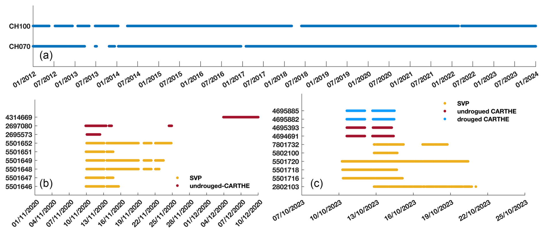
Figure A1 Mooring (a) and drifter (b, c) data are available for radar comparison from 1 February 2012 to 31 December 2023. The drifters, including the surface (drogued and undrogued CARTHE) and near-surface (SVP) types, were deployed in two periods: one in early November 2020 (b) and the other in early October 2023 (c). Only drifter data points that remained within the HF radar domain were used. The y axis displays the names of the observational instruments. Gaps denote missing data.

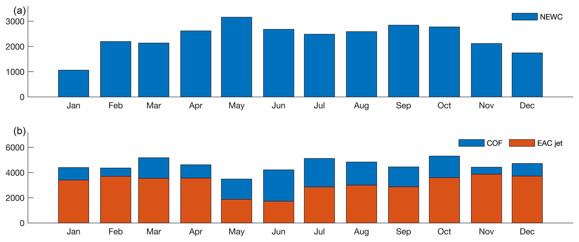
Figure A2 The number of hourly domain-averaged HF radar data available as a function of the month for each radar site: NEWC (a) and COF (b). The EAC jet bars (orange) represent the times that the jet was detected by the jet-following method from the COF data.

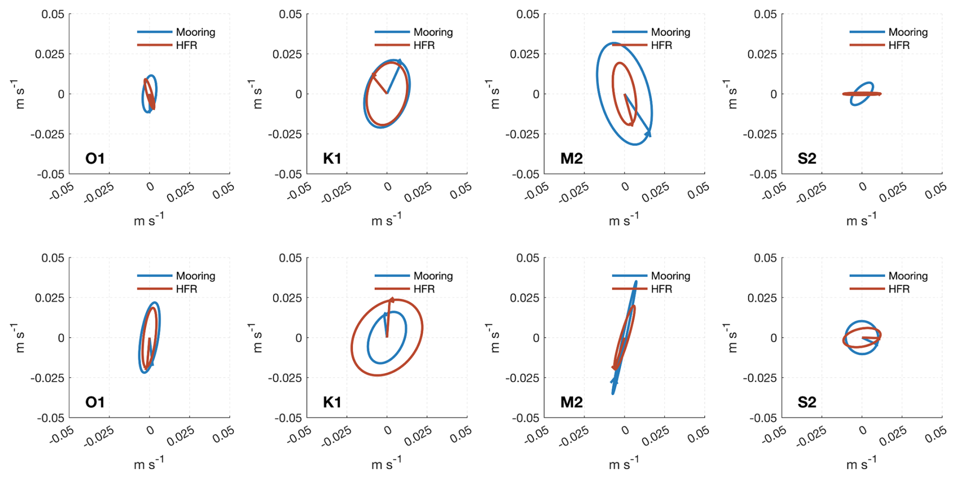
Figure A3 Tidal current ellipses extracted from the more than 1 year of mooring data and the HF radar-derived velocity at CH070 (15 November 2018 to 15 August 2020) and CH100 (from 15 February to 15 October 2019). The tidal phase (in UTC) is shown by corresponding lines.