SDUST2023VGGA: a global ocean vertical gradient of gravity anomaly model determined from multidirectional data from mean sea surface

Satellite altimetry is a vital tool for global ocean observation, providing critical insights into ocean gravity and its gradients. Over the past 6 years, satellite data from various space agencies have nearly tripled, facilitating the development of high-precision ocean gravity anomaly and ocean vertical gradient of gravity anomaly (VGGA) models. This study constructs a global ocean VGGA model named SDUST2023VGGA using multidirectional mean sea surface (MSS). To address computational limitations, the global ocean is divided into 72 sub-regions. In each sub-region, the DTU21 MSS model and the CNES-CLS22 mean dynamic topography (MDT) model are used to derive the geoid. To mitigate the influence of long-wavelength signals on the calculations, the study subtracts the long-wavelength geoid derived from the XGM2019e_2190 gravity field model from the (full-wavelength) geoid, resulting in a residual (short-wavelength) geoid. To ensure the accuracy of the VGGA calculations, a weighted least-squares method is employed using residual geoid data from a 17′×17′ area surrounding the computation point. This approach effectively accounts for the real ocean environment, thereby enhancing the precision of the calculation results. After combining the VGGA models for all sub-regions, the model's reliability is validated against the SIO V32.1 VGGA (named curv) model. The comparison between the SDUST2023VGGA and the SIO V32.1 model shows a residual mean is −0.08 Eötvös (E) and the RMS is 8.50 E, demonstrating high consistency on a global scale. Analysis of the differences reveals that the advanced data processing and modeling strategies employed in the DTU21 MSS model enable SDUST2023VGGA to maintain stable performance across varying ocean depths, unaffected by ocean dynamics. The effective use of multidirectional MSS allows for the detailed capture of ocean gravity field information embedded in the MSS model. Analysis across diverse ocean regions demonstrates that the SDUST2023VGGA model successfully reveals the internal structure and mass distribution of the seafloor. The SDUST2023VGGA model is freely available at https://doi.org/10.5281/zenodo.14177000 (Zhou et al., 2024).

1 Introduction

Gradients of gravity are the partial derivatives of the gravity vector components along the three axes of a Cartesian coordinate system. They describe spatial variations in the Earth's gravitational field, reflecting changes in both magnitude and direction. By enhancing high-frequency signals, gradients of gravity provide a detailed representation of subsurface density structures (Mortimer, 1977). This capability makes them valuable for accurately characterizing the spatial structure of field sources, understanding the Earth's internal structure, and identifying the location and depth of density variations (Romaides et al., 2001; Oruç, 2011; Panet et al., 2014). Consequently, gradients of gravity play a crucial role in geophysical exploration and ocean gravity field studies (Butler, 1984).

In recent years, the vertical gradient of gravity (VGG) has demonstrated significant potential across various disciplines, particularly in earthquake monitoring, underwater navigation, and ocean exploration. Fuchs et al. (2013) utilized gravity gradients from the Gravity field and Ocean Circulation Explorer (GOCE) satellite to detect substantial gravitational field changes resulting from the 2011 Tohoku earthquake in Japan, revealing that the observed gravity signal exceeded model predictions. This study highlighted the sensitivity and spatial correlation capabilities of gravity gradient technology in capturing seismic signals. Similarly, Wang et al. (2023) proposed a wavelet-transform-based regional matching method, advancing the application of gradients of gravity in underwater navigation and significantly improving matching accuracy. This work demonstrated the technology's practicality and precision. Furthermore, gradients of gravity inversion have proven to be a powerful tool in ocean exploration. Wan et al. (2023) combined satellite altimetry data with neural network techniques to predict global ocean depths, showcasing the broad applicability of gradients of gravity in oceanographic studies. Additionally, research by Kim and Wessel (2011) demonstrated that extracting short-wavelength information from satellite altimetry data effectively reveals the mass distribution of seafloor fracture zones and seamounts, providing new insights into geological structure analysis. These studies illustrate the diverse applications of gradients of gravity in earthquake monitoring, underwater navigation, bathymetry, and geological structure research.

As the application of gradients of gravity technology expands and gravity field theory evolves rapidly, gradients of gravity measurement techniques have seen continuous improvement (DiFrancesco et al., 2009; Stray et al., 2022; van der Meijde et al., 2015). However, measuring mobile gravity gradients remains costly, and achieving comprehensive global ocean coverage continues to be a challenge. The GOCE satellite, equipped with electrostatic accelerometer-based gravity gradiometers, provides global gravity data (Silvestrin et al., 2012; Rummel et al., 2011; Marks et al., 2013). Despite this, its resolution is limited in providing high-precision local gradients of gravity data (Novák et al., 2013).

In contrast, satellite altimetry technology has matured significantly and is now widely used to construct gravity potential models (Zingerle et al., 2020; Pavlis et al., 2012), mean sea surface (MSS) models (Andersen et al., 2023; Yuan et al., 2023), mean dynamic topography (MDT) models (Knudsen et al., 2021; Jousset et al., 2023, 2022), ocean gravity models (Sandwell and Smith, 2009; Sandwell et al., 2014; Garcia et al., 2014; Hwang et al., 1998; Hao et al., 2023; Zhu et al., 2022; Li et al., 2024), ocean gradient of gravity models (Bouman et al., 2011; Sandwell, 1992; Annan et al., 2024; Zhou et al., 2023), seafloor topography models (Smith and Sandwell, 1997; GEBCO Bathymetric Compilation Group, 2024; Hu et al., 2020), sea level studies (Schwatke et al., 2015; Vignudelli et al., 2019; Ablain et al., 2017), and monitoring changes in terrestrial lake water levels (Hwang et al., 2016; Sulistioadi et al., 2015). Among these, the MSS represents a relatively stable sea level. It is calculated by averaging instantaneous sea surface height measurements from satellite altimetry over a specific time period (Andersen and Knudsen, 2009). It is widely used to analyze ocean circulation, detect mesoscale eddies, assess sea level changes, determine geoid undulations, and identify crustal deformation. Additionally, the MSS has broad applications in geodesy, oceanography, geophysics, and climatology. In geodesy, it serves as a global reference for sea level, aiding in the study of geoid variations and helping to determine the precise locations of Earth's surface features and vertical crustal movements. In oceanography, the MSS is employed to study global ocean circulation, sea surface temperature, and changes in sea ice (Fu and Cheney, 1995; Vermeer and Rahmstorf, 2009; Skourup et al., 2017). In geophysics, it contributes to the analysis of the Earth's gravity field and seismic activity (Melini and Piersanti, 2006). In climatology, sea level data are fundamental for understanding the relationship between global sea level changes and climate change (Vermeer and Rahmstorf, 2009).

To fully extract the detailed ocean vertical gradient of gravity anomaly (VGGA) information embedded in the DTU21 MSS model, this study proposes a method for constructing a global VGGA model using multidirectional MSS data. Section 2 introduces the DTU21 MSS model and outlines the criteria for selecting additional datasets. Section 3 comprises two subsections: Sect. 3.1 outlines the strategy for partitioning the global ocean into sub-regions, describing how the ocean is divided based on geographic features and oceanographic dynamics, and Sect. 3.2 presents a newly developed method aimed at maximizing the extraction of ocean VGGA information from the DTU21 MSS model, thereby enhancing the effectiveness of gravity field data extraction. Section 4 evaluates the constructed model and assesses its reliability, and Sect. 5 discusses the factors influencing the model's construction results and key findings observed during the process. Section 7 presents the conclusions.

2 Research data

2.1 DTU21MSS

The DTU21 MSS model was developed by the National Space Institute of the Technical University of Denmark (DTU) (Andersen et al., 2023). The dataset is publicly available at https://data.dtu.dk/articles/dataset/DTU21_Mean_Sea_Surface/19383221 (last access: 8 January 2025). This model utilizes satellite altimetry data from multiple missions, including TOPEX/Poseidon, the Jason series, CryoSat-2, and SARAL/AltiKa, providing high-precision sea surface observations from 1 January 1993, to 31 December 2012.

To enhance the precision and resolution of the data, the DTU21 MSS model employs a new processing chain that incorporates advanced filtering and editing techniques. Compared to its predecessors, DTU15MSS and DTU18MSS, which were constructed using 1 Hz satellite altimetry data, DTU21 MSS is based on 2 Hz data, significantly improving its accuracy. The integration of satellite altimetry data with advanced retracking techniques and the application of the Parks–McClellan filtering algorithm during the development of the DTU21 MSS model enabled enhanced resolution in the 10–40 km wavelength range, significantly improving accuracy in polar and coastal regions.

The DTU21 MSS dataset is provided in a gridded format. By combining data from multiple satellite sources and utilizing advanced processing methods, the DTU21 model delivers high spatial resolution and precision on a global scale, making it a reliable resource for oceanographic and Earth science research.

2.2 CNES-CLS22 MDT

To extract geoid information from the MSS model, a MDT model is required. The CNES-CLS22 MDT, with a resolution of 7.5′×7.5′, was derived by integrating data from satellite altimetry; GRACE and GOCE gravity missions; and in situ oceanographic measurements, such as drifter velocities, high-frequency radar velocities, and salinity–temperature profiles (Jousset et al., 2023). The dataset is accessible at https://www.aviso.altimetry.fr/en/data/products/auxiliary-products/mdt/mdt-global-cnes-cls.html (last access: 8 January 2025).

Compared to its predecessor, CNES-CLS18 MDT, the CNES-CLS22 MDT demonstrates significant improvements in high-latitude regions. It offers broader coverage and eliminates artifacts, primarily due to the use of a new initial estimate that incorporates the CNES-CLS22 MSS and the GOCO06s geoid model. Additionally, optimal filtering techniques, such as Lagrangian filtering in coastal areas, were applied to further enhance accuracy.

The selection of the CNES-CLS22 MDT ensures minimal correlation with the DTU21 MSS (Knudsen et al., 2022, 2021), making it more effective for extracting detailed ocean gravity field information embedded in the MSS model. This choice enhances the credibility of the VGGA model developed in this study.

2.3 XGM2019e

A highly accurate Earth gravity field model is essential for applying the remove–restore method. In this study, the reference gravity field model XGM2019e_2190 was selected due to its widespread use in geoscience research and practical applications. The model is available from the International Center for Global Earth Models (ICGEM) at https://icgem.gfz-potsdam.de/home (last access: 8 January 2025) (Ince et al., 2019).

XGM2019e is a comprehensive global gravity field model, complete to degree and order 5399, offering a half-wavelength resolution of approximately 4 km. In this study, the XGM2019e_2190 model, truncated to degree and order 2190, is utilized. It is primarily based on the GOCO06s satellite gravity field model, supplemented by a 15 min terrestrial gravity dataset and a 1 min enhanced gravity dataset provided by the US National Geospatial-Intelligence Agency (Zingerle et al., 2020). The integration of satellite and ground-based gravity data ensures high precision in both large-scale and local gravity field representations, making XGM2019e suitable for detailed geophysical studies, including oceanography, tectonics, and geoid determination.

The model's high resolution and accuracy are critical for improving the reliability of the VGGA model developed in this study. Using XGM2019e_2190 in the remove–restore process, the long-wavelength components of the gravity field are efficiently removed, allowing for focused extraction of the high-frequency VGGA from the MSS model.

2.4 SIO V32.1

Given the significant challenges in obtaining in situ measurements of VGGAs over the oceans, this study utilized the SIO V32.1 dataset, derived from satellite altimetry data, to validate its results. The SIO V32.1 dataset is a high-precision, high-resolution global ocean dataset that includes models for the VGGA, gravity anomaly, and the north–south and east–west components of the deflection of the vertical (DOV) (Garcia et al., 2014). The latest version, V32.1, also incorporates an MSS model.

The SIO V32.1 dataset has been widely used in geophysical and oceanographic studies due to its ability to provide detailed gravity field information over oceanic regions, which is difficult to achieve using traditional measurement techniques. The combination of satellite altimetry data and advanced processing algorithms allows for high spatial resolution, making this dataset particularly useful for detecting fine-scale oceanic structures, including seamounts, fracture zones, and variations in seafloor topography. Using the SIO V32.1 dataset for cross-validation ensures the robustness and reliability of the VGGA model developed in this study.

2.5 GEBCO bathymetric model

To evaluate the performance of the SDUST2023VGGA model under different bathymetric conditions, this study employs the General Bathymetric Chart of the Oceans (GEBCO) bathymetric model. The first objective is to assess the performance of SDUST2023VGGA in various seafloor topographies. The second objective is to evaluate the correlation between the GEBCO model and SDUST2023VGGA, particularly examining whether VGGAs can explain seafloor topography. The GEBCO model is widely recognized in the field of geosciences for its detailed representation of the seafloor topography of the world's oceans and is available on the GEBCO project website (https://www.gebco.net/data_and_products/gridded_bathymetry_data/, last access: 8 January 2025).

The GEBCO bathymetric model combines ship-based bathymetric surveys and satellite-derived altimetric data. It provides a global, high-resolution depiction of seafloor depth. The current version, GEBCO2024, has a spatial resolution of 15 arcsec, which is approximately equivalent to 450 m at the Equator. This high resolution allows for the identification of various seafloor features, such as seamounts, trenches, and ridges, thereby supporting a wide range of geophysical and oceanographic studies.

3 Research methods

3.1 Global zoning strategy

To overcome computational limitations, a regionalized global modeling approach was adopted. The global ocean was divided into multiple sub-regions, each computed independently and then merged into a unified global model. Between 60° S and 60° N, each sub-region was defined as a 30°×30° grid. Beyond these latitudes, the grid size was adjusted to 30°×20° to account for the unique geographic characteristics of high-latitude regions. As shown in Fig. 1, sub-regions were systematically labeled: horizontally, they were labeled L1 to L12 starting from 0° longitude and moving eastward; vertically, they were labeled B1 to B6 starting from 80° S and moving northward.

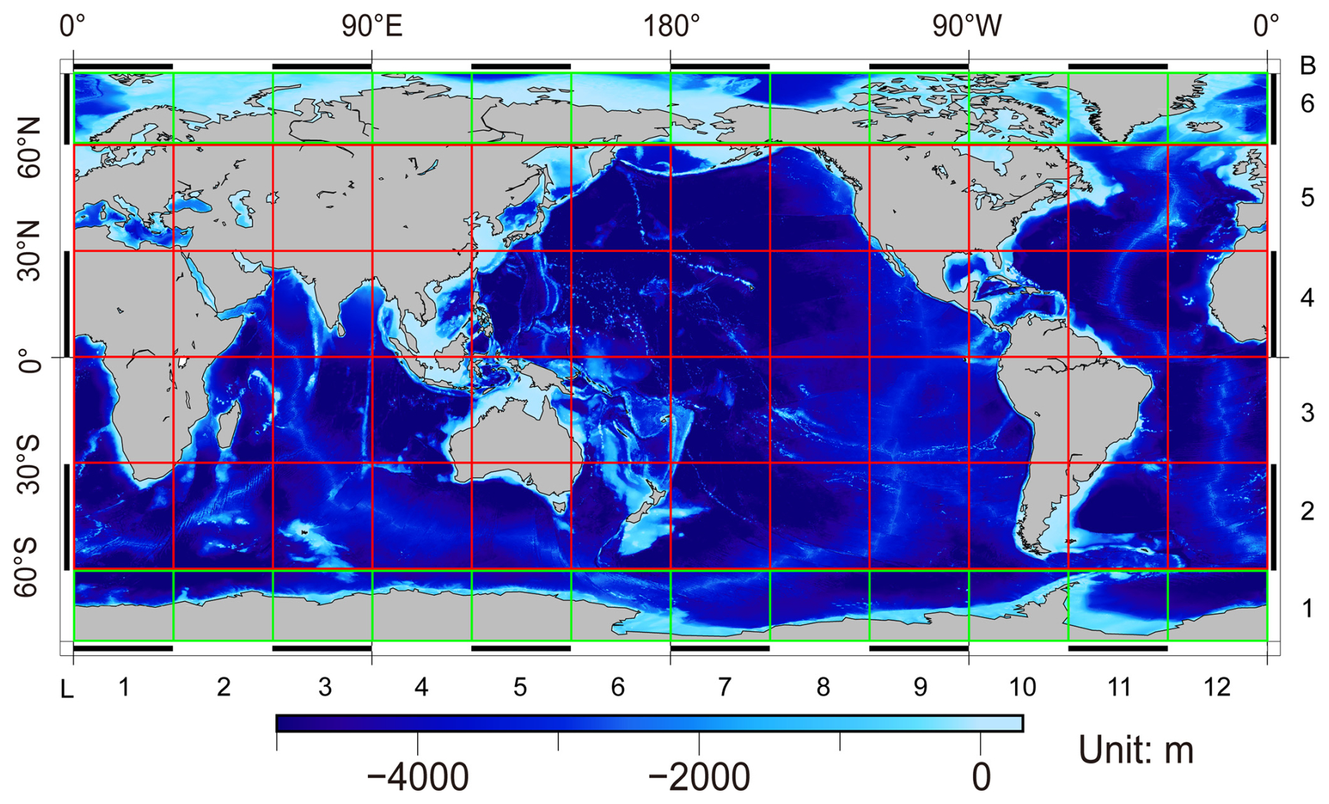
Figure 1 Global oceanic partition strategy using 30°×30° and 30°×20° grids based on the regionalized global modeling approach. Sub-regions are labeled as L1 to L12 (horizontal) and B1 to B6 (vertical) for identification.

To mitigate edge effects during derivative calculations, each sub-region was extended with an excluded margin. For standard 3°×30° sub-regions, the MSS and MDT models were expanded to a 32°×32° area to include these margins. After constructing the VGGA model for the extended region, the excluded margins were clipped, leaving the core 30°×30° sub-region, as illustrated in Fig. 2. This clipping strategy preserved critical boundary information during derivative calculations, effectively reducing edge effects and enhancing the accuracy of the final model. By temporarily extending sub-region boundaries where possible, the loss of important edge data was minimized, ensuring reliable results in VGGA computations. This approach significantly improves the model's precision, particularly at sub-region boundaries.

Figure 2 Clipping strategy to mitigate edge effects. The example illustrates a 30°×30° sub-region expanded to 32°×32° during computation. The excluded margins are clipped after processing, leaving the retained region for accurate results.

3.2 Model building

The VGG consists of two components: the vertical gradient of normal gravity and the VGGA. In this study, the VGGA is derived from the MSS model. Since the vertical gradient of normal gravity is a latitude-dependent function, the VGGA alone suffices to reveal Earth's internal structure. Therefore, only the VGGA was computed in this research, excluding the vertical gradient of normal gravity. The VGGA represents the difference between the gradient of actual gravity and normal gravity, emphasizing deviations caused by factors such as uneven mass distribution, topographical variations, and subsurface structures. These deviations provide valuable insights into geological formations and geophysical characteristics beneath the Earth's surface.

Assuming the disturbing potential, denoted as T, is at a point on the geoid, the gravity anomaly is computed using the fundamental equations of physical geodesy (Moritz, 1980; Hofmann-Wellenhof and Moritz, 2006):

$$\begin{array}{}\text{(1)}& \mathrm{\Delta }g=-{\displaystyle \frac{\partial T}{\partial h}}+{\displaystyle \frac{\mathrm{1}}{\mathit{\gamma }}}{\displaystyle \frac{\partial \mathit{\gamma }}{\partial h}}T,\end{array}$$

where Δg denotes the gravity anomaly, γ is the normal gravity at the point, and h is the orthometric height. For a spherical approximation of the ellipsoid, the following relationship holds:

$$\begin{array}{}\text{(2)}& {\displaystyle \frac{\partial }{\partial h}}\cong {\displaystyle \frac{\partial }{\partial r}}.\end{array}$$

According to Bruns' formula, γ can be replaced by G, leading to the following relationship outside the Earth:

$$\begin{array}{}\text{(3)}& \mathrm{\Delta }g=-{\displaystyle \frac{\partial T}{\partial r}}-{\displaystyle \frac{\mathrm{2}}{r}}T.\end{array}$$

By differentiating Eq. (3) and applying Laplace's equation (∇²U=0), the vertical derivative of the gravity anomaly can be expressed in terms of its horizontal derivatives. This results in the following formula for calculating the VGGA, which incorporates the geoid as well as its first and second horizontal derivatives:

$$\begin{array}{}\text{(4)}& {\displaystyle \frac{\partial \mathrm{\Delta }g}{\partial r}}={\displaystyle \frac{\mathrm{2}G}{R^{\mathrm{2}}}}N-{\displaystyle \frac{G}{R^{\mathrm{2}}}}\tan \mathit{\phi }{\displaystyle \frac{\partial N}{\partial \mathit{\phi }}}+{\displaystyle \frac{G}{R^{\mathrm{2}}}}{\displaystyle \frac{{\partial }^{\mathrm{2}}N}{\partial {\mathit{\phi }}^{\mathrm{2}}}}+{\displaystyle \frac{G}{R^{\mathrm{2}}{\cos }^{\mathrm{2}}\mathit{\phi }}}{\displaystyle \frac{{\partial }^{\mathrm{2}}N}{\partial {\mathit{\lambda }}^{\mathrm{2}}}},\end{array}$$

where N represents the geoid height, G is the mean gravity, φ is the geographic latitude, and λ is the geographic longitude.

This equation demonstrates how the VGGA is a direct function of the geoid height (N) as well as its first and second derivatives in the latitude (φ) and longitude (λ) directions. The coupling of horizontal and vertical derivatives is a direct consequence of Laplace's equation, ensuring that the short-wavelength components in the vertical direction are determined entirely by the horizontal variations of the geoid.

After establishing the regional partitioning strategy and deriving the method for calculating the VGGA, the CNES-CLS22 MDT model was interpolated onto the DTU21 MSS grid using cubic spline interpolation to increase the resolution. This increased the resolution to ${\mathrm{1}}^{\prime }\times {\mathrm{1}}^{\prime }$ and ensured consistency between the two datasets. The choice of cubic spline interpolation was based on its superior ability to provide smooth and continuous estimates, which is essential for accurately capturing the fine-scale geoid variations. This interpolation step enhances the spatial detail of the MDT, facilitating more precise geoid extraction. Subsequently, the interpolated MDT model was subtracted from the DTU21 MSS model to obtain the geoid, denoted by N:

$$\begin{array}{}\text{(5)}& N=\mathrm{MSS}-{\mathrm{MDT}}_{\mathrm{inter}}.\end{array}$$

Next, the remove–restore method was employed to isolate the short-wavelength residual geoid by subtracting the long-wavelength component, represented by the XGM2019e_2190 geoid, from the full-wavelength geoid. This process separates the geoid into its long- and short-wavelength components. By removing the long-wavelength signals, the short-wavelength residual geoid highlights local variations and finer details in the geoid (Hwang, 1999):

$$\begin{array}{}\text{(6)}& N_{\mathrm{res}}=N-N_{\mathrm{ref}},\end{array}$$

where N_res denotes the short-wavelength residual geoid, N represents the full-wavelength geoid, and N_ref represents the long-wavelength component derived from the XGM2019e_2190 geoid.

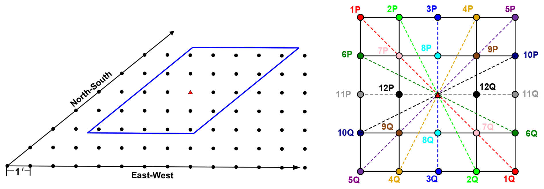
Figure 3 Illustration of the north–south and east–west components of the derivative of the residual geoid based on multidirectional MSS data, using a 5′×5′ window as an example. The red triangle represents the center point for calculation, and P–Q pairs indicate 12 possible combinations used for multidirectional gradient computation.

Through the remove–restore method, the gridded MSS data were used to derive the residual geoid, N_res. The long-wavelength signals, primarily influenced by the Earth's geopotential field, were removed from the MSS using a reference geoid model, leaving the residual geoid that captures shorter-wavelength features associated with local oceanographic and topographic variations. For each calculation point, the second-order derivatives of N_res were computed in multiple directions using a weighted least-squares method. This approach allowed for the extraction of detailed gravity field information by calculating the second-order partial derivatives in the north–south and east–west components. The weighted least-squares method ensured that the calculations accounted for the complexity of ocean topography, enhancing the accuracy and reliability of the derived gravity field information. The following equation was used for the calculation:

$$\begin{array}{}\text{(7)}& \begin{array}{rl}{\displaystyle \frac{{\partial }^{\mathrm{2}}{N}_{\mathrm{res},(kP,kQ)}}{\partial l^{\mathrm{2}}}}& ={\displaystyle \frac{{\partial }^{\mathrm{2}}{N}_{\mathrm{res},(kP,kQ)}}{\partial {\mathit{\phi }}^{\mathrm{2}}}}{\cos }^{\mathrm{2}}{a}_{kP,kQ}\\ & +\mathrm{2}{\displaystyle \frac{{\partial }^{\mathrm{2}}{N}_{\mathrm{res},(kP,kQ)}}{\partial \mathit{\phi }\partial \mathit{\lambda }}}\sin a_{kP,kQ}\cos a_{kP,kQ}\\ & +{\displaystyle \frac{{\partial }^{\mathrm{2}}{N}_{\mathrm{res},(kP,kQ)}}{\partial {\mathit{\lambda }}^{\mathrm{2}}}}{\sin }^{\mathrm{2}}{a}_{kP,kQ},\end{array}\end{array}$$

where k represents the number of equations, α is the geodetic azimuth between points P and Q, and l denotes the horizontal distance between these two points. A calculation window size of ${\mathrm{17}}^{\prime }\times {\mathrm{17}}^{\prime }$ was determined. For a given calculation window size of $i^{\prime }\times i^{\prime }$, the number of equations is calculated as $k=(i^{\mathrm{2}}-\mathrm{1})/\mathrm{2}$. For example, when i=5, 12 sets of second-order derivatives of N_res are obtained, resulting in 12 equations.

Figure 3 illustrates the calculation process using a ${\mathrm{5}}^{\prime }\times {\mathrm{5}}^{\prime }$ calculation window. In the actual computations, a larger ${\mathrm{17}}^{\prime }\times {\mathrm{17}}^{\prime }$ window was employed to ensure sufficient coverage and improve the accuracy of the gradient extraction.

The matrix form of Eq. (7) can be represented as

$$\begin{array}{}\text{(8)}& \mathit{V}=\mathbf{A}\mathit{X}-\mathbf{L},\end{array}$$

where V represents the residual vector and A denotes the coefficient matrix composed of the north–south and east–west second-order partial derivatives:

$$\begin{array}{}\text{(9)}& \begin{array}{rl}& \mathbf{A}=\\ & \left(\begin{array}{lll}{\cos }^{\mathrm{2}}{\mathit{\alpha }}_{\mathrm{1}P,\mathrm{1}Q}& \mathrm{2}\sin {\mathit{\alpha }}_{\mathrm{1}P,\mathrm{1}Q}\cos {\mathit{\alpha }}_{\mathrm{1}P,\mathrm{1}Q}& {\sin }^{\mathrm{2}}{\mathit{\alpha }}_{\mathrm{1}P,\mathrm{1}Q}\\ {\cos }^{\mathrm{2}}{\mathit{\alpha }}_{\mathrm{2}P,\mathrm{2}Q}& \mathrm{2}\sin {\mathit{\alpha }}_{\mathrm{2}P,\mathrm{2}Q}\cos {\mathit{\alpha }}_{\mathrm{2}P,\mathrm{2}Q}& {\sin }^{\mathrm{2}}{\mathit{\alpha }}_{\mathrm{2}P,\mathrm{2}Q}\\ {\cos }^{\mathrm{2}}{\mathit{\alpha }}_{\mathrm{3}P,\mathrm{3}Q}& \mathrm{2}\sin {\mathit{\alpha }}_{\mathrm{3}P,\mathrm{3}Q}\cos {\mathit{\alpha }}_{\mathrm{3}P,\mathrm{3}Q}& {\sin }^{\mathrm{2}}{\mathit{\alpha }}_{\mathrm{3}P,\mathrm{3}Q}\\ \mathrm{⋮}& \mathrm{⋮}& \mathrm{⋮}\\ {\cos }^{\mathrm{2}}{\mathit{\alpha }}_{(k-\mathrm{1})P,(k-\mathrm{1})Q}& \mathrm{2}\sin {\mathit{\alpha }}_{(k-\mathrm{1})P,(k-\mathrm{1})Q}\cos {\mathit{\alpha }}_{(k-\mathrm{1})P,(k-\mathrm{1})Q}& {\sin }^{\mathrm{2}}{\mathit{\alpha }}_{(k-\mathrm{1})P,(k-\mathrm{1})Q}\\ {\cos }^{\mathrm{2}}{\mathit{\alpha }}_{kP,kQ}& \mathrm{2}\sin {\mathit{\alpha }}_{kP,kQ}\cos {\mathit{\alpha }}_{kP,kQ}& {\sin }^{\mathrm{2}}{\mathit{\alpha }}_{kP,kQ}\end{array}\right).\end{array}\end{array}$$

X is a vector containing the second-order partial derivatives of the residual geoid in the north–south and east–west components. Once the residual vector V and the coefficient matrix A are established, the weighting matrix is applied to balance data contributions from different directions. The solution for X, corresponding to the second-order partial derivatives of the residual geoid, is determined by minimizing the cost function Ψ=V^TWV. The solution is given by

$$\begin{array}{}\text{(10)}& \mathit{X}={\left({\mathbf{A}}^T\mathbf{WA}\right)}^{-\mathrm{1}}\left(\mathbf{AW}\mathit{V}\right),\end{array}$$

where W is the weighting matrix, calculated using an inverse distance formula: $\mathbf{W}=\mathrm{diag}\left(\frac{\mathrm{1}}{l_{\mathrm{1}}^{\mathrm{2}}},\frac{\mathrm{1}}{l_{\mathrm{2}}^{\mathrm{2}}},\mathrm{\dots },\frac{\mathrm{1}}{l_n^{\mathrm{2}}}\right)$. This formula gives higher weights to closer points, thereby balancing data contributions and ensuring accuracy and reliability in the results.

After computing the residual VGGAs, they were combined with the long-wavelength component of the VGGA from the XGM2019e_2190 model as part of the remove–restore process. This step was crucial to mitigate the influence of long-wavelength signals, which could distort the calculation of finer, short-wavelength variations in the geoid. As a result, the resulting VGGA models accurately captured short-wavelength geoid variations while effectively excluding long-wavelength signals.

To address boundary effects, the edges of each sub-region were initially expanded. This expansion was necessary to suppress edge artifacts during calculations. Subsequently, the expanded regions were clipped to remove overlaps, ensuring that only the valid central area of each sub-region was retained. Once this step was completed, the VGGA models for each sub-region were prepared for comparison with existing models and for merging into a continuous global model.

In contrast to this study, which calculates the VGGA by deriving the second-order horizontal partial derivatives of the geoid, the VGGA model in SIO V32.1 curv is computed using the first-order derivatives of the DOV's north–south and east–west components (Muhammad et al., 2010; Sandwell and Smith, 1997, 2009). To evaluate and validate the accuracy of the proposed method, the VGGA model constructed in this study was compared with the SIO V32.1 curv.

Figure 4 Workflow for constructing the VGGA model using the DTU21 MSS, CNES-CLS22 MDT, and XGM2019e_2190.

Following the computation and validation of each sub-region, these sub-regions were merged to construct a continuous marine VGGA model spanning from 80° S to 80° N, designated as SDUST2023VGGA.

The workflow of the study is illustrated in Fig. 4.

4 Results and analysis

After establishing the regional partitioning strategy, the DTU21 MSS was utilized, and the CNES-CLS22 MDT was subtracted to derive the geoid height. The XGM2019e_2190 gravity field model was subsequently subtracted to obtain the residual geoid. A multidirectional approach was applied to the geoid height data to calculate the second-order partial derivatives, and the VGGA for each sub-region was derived using the weighted least-squares method. These sub-regional VGGA models were integrated to construct a global VGGA model for oceanic regions.

Due to the limited availability of direct global VGGA observations, the satellite-altimetry-based SIO V32.1 curv model served as a reference for comparison. The inversion statistics for each sub-region are presented in Table 1 presents the inversion statistics for each sub-region, highlighting discrepancies between the curv and VGGA models. The differences between the two models were analyzed to assess and validate the accuracy of the computational method used in this study.

Table 1 Statistical RMS differences obtained by subtracting the constructed SDUST2023VGGA model from the SIO V32.1 curv model (in E).

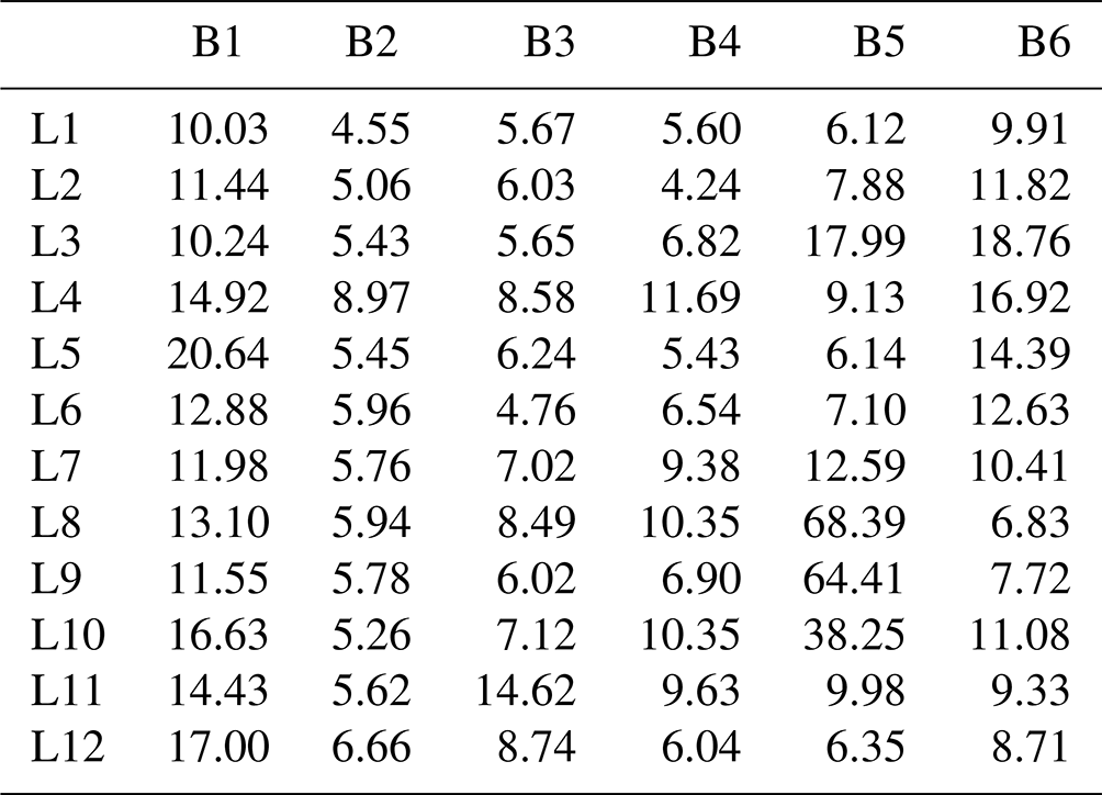
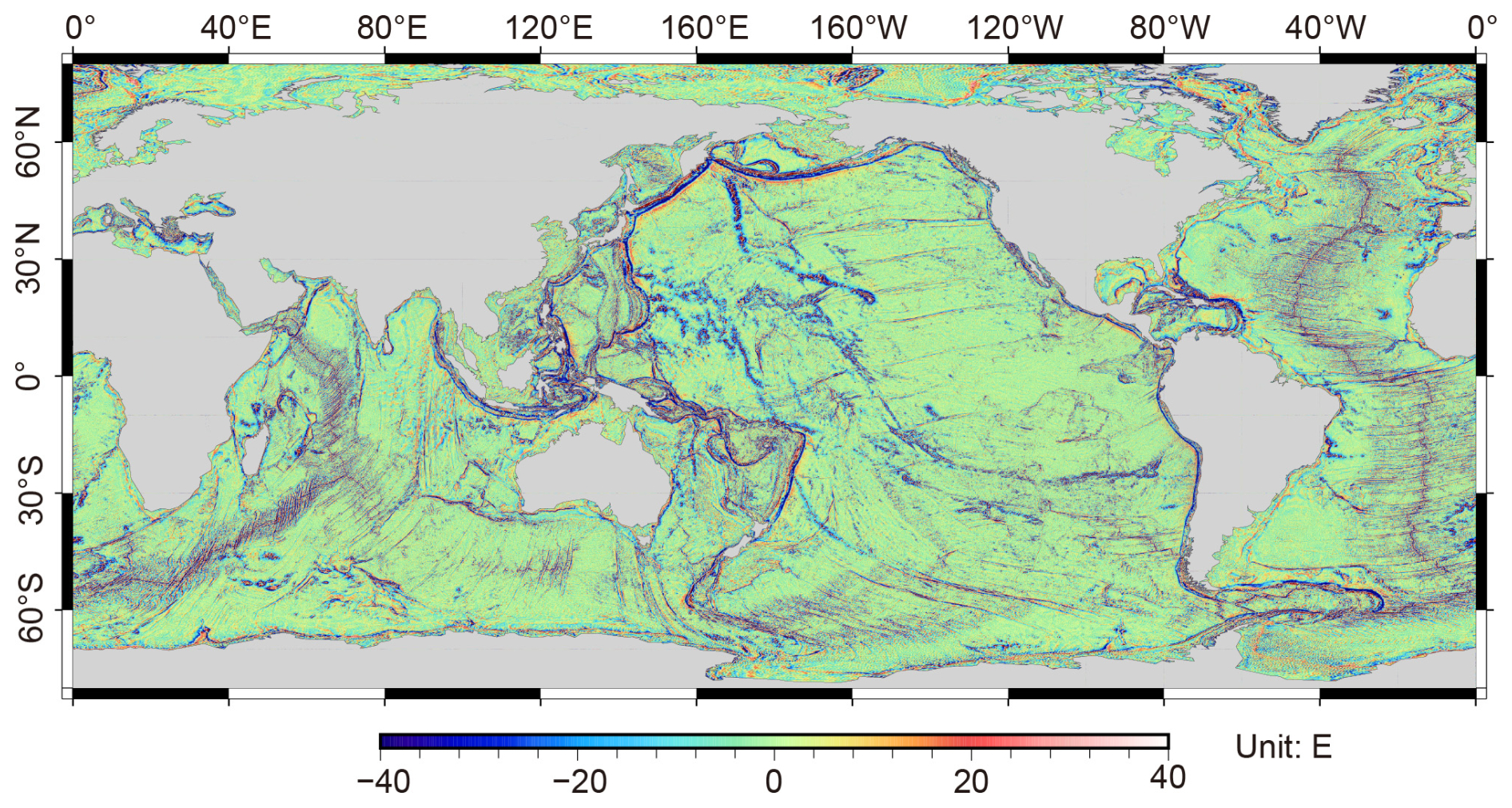
Figure 5 Global VGGA model SDUSTVGGA constructed from the DTU21 MSS.

The analysis of the RMS differences in Table 1 reveals significant variability along both longitudinal (L1 to L12) and latitudinal (B1 to B6) directions. Longitudinally, no clear trend is observed, indicating that VGGA discrepancies are influenced by diverse geographical and geophysical factors, such as seafloor topography and local tectonics. In the latitudinal direction, lower RMS values are evident in equatorial regions (B3 and B4), which likely benefit from high-quality satellite altimetry data. Conversely, sub-region B6 exhibits higher RMS values, particularly in L3, L4, and L5, reflecting the complex bathymetric features and tectonic activity characteristic of sub-polar regions.

Further analysis, in conjunction with the ocean depth model (Fig. 1), suggests that significant VGGA variations near the Equator are linked to deep ocean trenches, mid-ocean ridges, and other major geological structures that strongly influence the Earth's mass distribution. Longitudinally, sub-regions such as L1, L2, and L6 generally exhibit lower RMS differences across most latitude bands, suggesting more homogeneous geoid characteristics in these regions.

Upon completing the model construction for all sub-regions, the excess portions were trimmed to produce a continuous global VGGA model for oceanic regions, designated as SDUST2023VGGA (hereafter referred to as SDUSTVGGA). The final model spans longitudes from 0 to 360° and latitudes from 80° S to 80° N. Figure 5 illustrates the resulting global VGGA model.

Investigating Earth's tectonic activities and their impact on gravitational fields enhances our understanding of geophysical dynamics. Supported by the visualizations in Fig. 5, this study examines key tectonic features, including mid-ocean ridges, abyssal plains, subduction zones, and volcanically active regions. These features play pivotal roles in shaping the Earth's landscape and influencing the observed patterns of VGGAs. The discussions that follow analyze how these features contribute to gravity field variations and their implications for understanding underlying geodynamic processes.

Mid-ocean ridges, representing divergent boundaries in the global plate tectonic system, are prominent features. Notable examples include the Mid-Atlantic Ridge and the East Pacific Rise, both characterized by mantle upwelling, where magma rises and solidifies to form new oceanic crust. This process results in localized density reduction, creating a stark contrast with the surrounding older, cooler oceanic crust and leading to pronounced gravity field variations (Álvarez et al., 2018; Michael and Cornell, 1998; Escartín et al., 2009). For instance, the Mid-Atlantic Ridge, extending from Iceland (65° N, 18° W) to the South Atlantic (40° S, 10° W), appears as a linear high-gradient region on the gradient map, reflecting crustal changes due to mantle upwelling and expansion (Rao et al., 2004). Similarly, the East Pacific Rise, located in the eastern Pacific and trending southwestward from 55° S, 130° W, is characterized by significant volcanic activity and hydrothermal vents, contributing to crustal expansion and VGGAs (Yu et al., 2022).

Deep-sea plains, typically linked to plate subsidence, where the oceanic crust gradually sinks under its weight, result in relatively stable gradient. The Pacific abyssal plain, extending from approximately 30° N to 60° S and spanning longitudes from 150° W to 150° E, is characterized by a relatively thin crust and smooth, low-gradient regions on the map. This uniformity is influenced by low-density, fine-grained sediments, such as silt and clay, that cover the plain, minimizing variations in crustal density (Smith and Sandwell, 1997; Clift and Vannucchi, 2004). Similarly, the Atlantic abyssal plains, primarily distributed between 40° N and 60° S and from 30° W to 30° E, display low VGGA due to similar sedimentary characteristics, which dampen tectonic activity and stabilize the crust. The Indian Ocean abyssal plains, located between 30 and 60° S and spanning longitudes from 60 to 100° E, exhibit comparable low gradients, highlighting the effects of thick, fine-grained sediment deposits in maintaining crustal stability.

Subduction zones, where one tectonic plate is forced beneath another, are areas of dramatic changes in crustal density that generate distinct low VGGAs. For instance, the Mariana Trench, located at 11° N, 142° E, is the world's deepest oceanic trench, with the Challenger Deep reaching a depth of 10 994 m. The extreme pressure at these depths increases water density by nearly 5 %, significantly influencing gravity field variations. These effects are represented as dark-blue areas in Fig. 5, indicating low VGGAs (Han et al., 2018). Similarly, the Peru–Chile Trench, situated at approximately 23° S, 71° W, marks the subduction of the Nazca Plate beneath the South American Plate. This tectonic process generates significant seismic and volcanic activity, contributing to notable low VGGAs in the region (Álvarez et al., 2018).

Volcanically active zones, characterized by crustal uplift, fractures, and magma activity, show localized high VGGAs due to the presence of magma chambers and fault zones. For example, the Hawaiian volcanic chain, spanning from 18 to 29° N and 155 to 172° W, is a hotspot-driven volcanic chain with notable VGGAs caused by magma upwelling (Poland and Carbone, 2016). Similarly, the Galápagos volcanic chain, spanning from 0° N, 89° W to 1° N, 92° W, experiences significant volcanic activity driven by the Galápagos hotspot, with localized density variations contributing to high VGGAs (Vigouroux et al., 2008). The New Zealand Volcanic Arc, situated at the convergence of the Pacific and Indo-Australian plates (35 to 39° S, 175 to 179° E), displays similar high gradients associated with subsurface magma activity and crustal thickness variations. These regions exemplify how volcanic and tectonic dynamics interact to shape localized gravity anomaly patterns.

The SDUSTVGGA map reveals crucial density variations within the crust and mantle, providing an indispensable tool for identifying geological structures, exploring mineral resources, and assessing seismic and volcanic risks. The findings from this analysis emphasize the utility of VGGAs in elucidating tectonic and volcanic processes on a global scale.

Given the challenges in obtaining direct VGGA measurements, the reliability of the SDUSTVGGA model was assessed by comparison with the SIO V32.1 curv model. The differences between the SDUSTVGGA model and the SIO V32.1 curv model produced a residual model, illustrated in Fig. 6. The SIO V32.1 curv model, based on satellite altimetry data, serves as a robust reference for cross-validation.

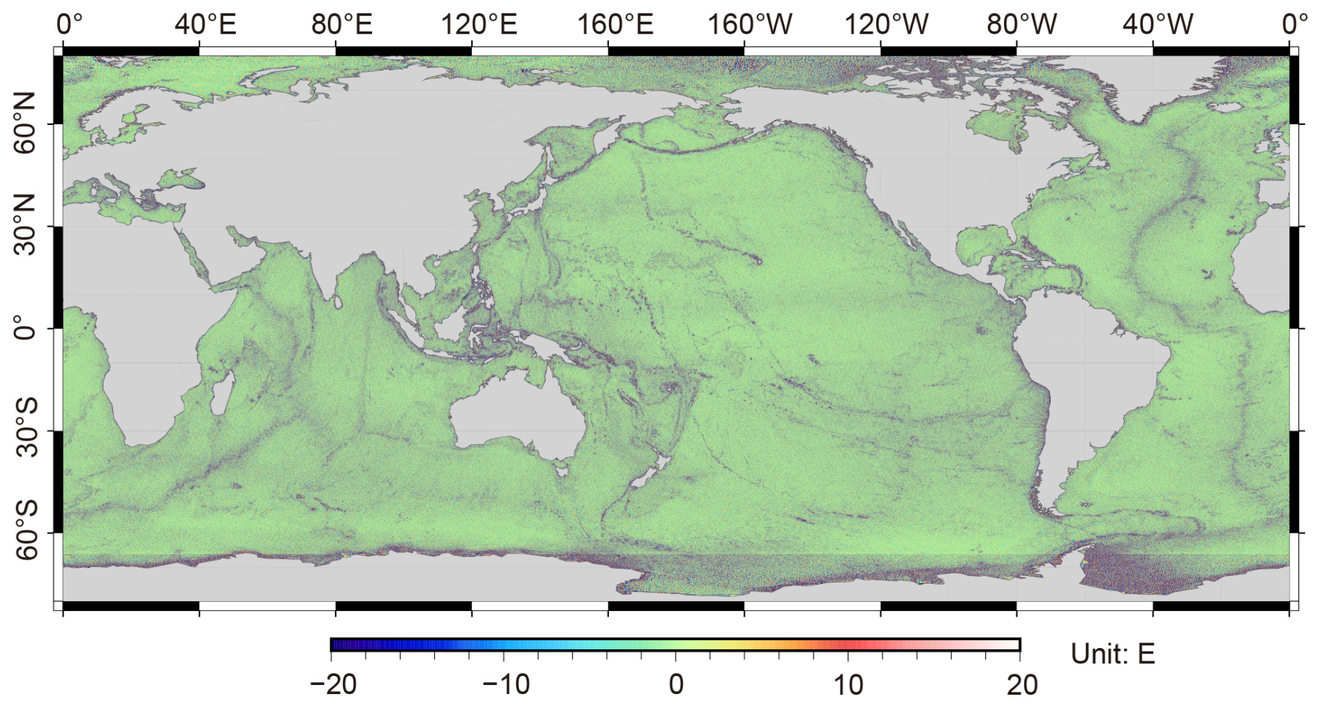
Figure 6 The spatial distribution of differences obtained by subtracting the SDUSTVGGA model from the SIO V32.1 curv model.

Figure 6 presents the global spatial distribution of differences between the SDUSTVGGA model and the SIO V32.1 curv model. In most regions, the two models demonstrate strong consistency, exhibiting generally low residuals across the oceans. This consistency is particularly evident in mid-latitudes and low latitudes, where satellite altimetry data tends to be more accurate and less affected by atmospheric or sea-ice interference. Furthermore, increased differences between the models are evident from 66 to 80° S, with a distinct seam appearing at 66° S. This seam likely arises from differences in data quality and processing methods applied to polar regions, underscoring the challenges in these areas.

To mitigate the impact of outliers and better assess data quality, a two-step filtering process was applied independently to the original data during the analysis of residual differences between the two models. Here, σ represents the standard deviation (SD), measuring the dispersion of data points from the mean. First, a 10-fold SD (10σ) filter was applied to the original data to exclude extreme outliers, which removed 0.07 % of the data. Following this, a stricter 3-fold SD (3σ) filter was applied, again to the original data that targeted moderate outliers and removed 1.41 % of the data. This hierarchical filtering approach refined the residuals by excluding outliers, facilitating a more detailed and accurate analysis of the model's accuracy and robustness. The statistical information and histogram of the residual differences are presented in Table 2 and Fig. 7, respectively.

Table 2 Statistical differences obtained by subtracting the SDUSTVGGA model from the SIO V32.1 curv model (in E).

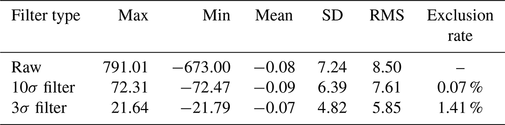
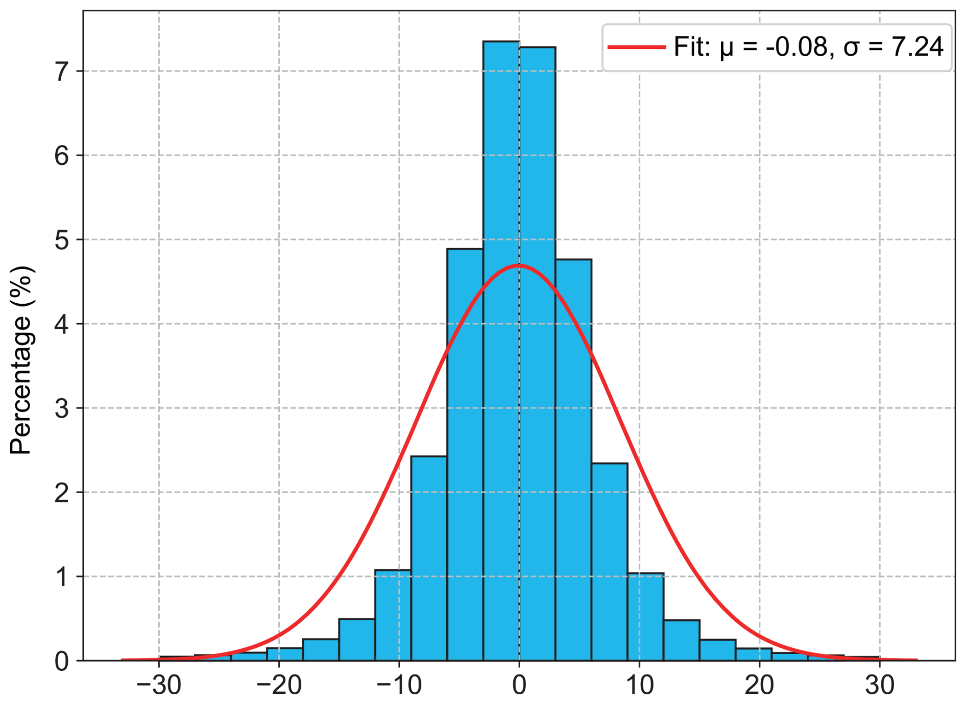
Figure 7 The histogram of differences obtained by subtracting the SDUSTVGGA model from the SIO V32.1 curv model, with fit parameters μ representing the mean and σ representing the SD.

Globally, the SDUSTVGGA model derived from multidirectional MSS data shows strong consistency with the SIO V32.1 curv model. Initial statistical analysis of the model differences revealed a maximum of 791.01 E and a minimum of −673.00 E, with a mean of −0.08 E, indicating an approximately symmetric distribution centered around zero. The SD was 7.24 E, and the RMS was 8.50 E, suggesting the presence of outliers, potentially resulting from satellite altimetry limitations in coastal areas and regions with complex seafloor topography.

To assess the impact of outliers on the statistical metrics, data points deviating by more than ±10 and ±3 times the SD from the mean were progressively removed, followed by a re-analysis of the remaining dataset. After excluding data points exceeding ±10 times the SD, the maximum and minimum values were reduced to 72.31 and −72.47 E, respectively, while the mean remained at −0.09 E. This indicates that extreme outliers significantly impacted the SD and RMS error; however, since these outliers represented only 0.07 % of the total data, their effect on the mean was minimal.

Further exclusion of data points deviating by more than ±3 times the SD (1.41 % of the data) reduced the maximum and minimum values to 21.64 and −21.79 E, with the mean shifting slightly to −0.07 E. This demonstrates that removing more outliers led to a continued decrease in the SD and RMS error, indicating reduced data dispersion and an improved fit. Nevertheless, the stability of the mean suggests that the core results were robust despite the presence of outliers. This stability implies that the underlying model retains its predictive capacity and reliability even when outliers are present, which is crucial for ensuring the robustness of the SDUSTVGGA model in diverse oceanic regions.

5 Discussion

5.1 Validation and analysis of model performance

Coastlines and islands can contaminate altimetry waveform data (Guo et al., 2010), which significantly affects the accuracy of altimetry measurements and, consequently, the inversion results of gradients of gravity anomaly. In deep-sea regions, complex ocean dynamics such as deep currents, internal waves, and eddies substantially impact sea surface morphology by causing undulations and localized changes in sea surface height (Khaki et al., 2015). Additionally, the satellite's orbital inclination affects its coverage of different latitudinal regions, potentially resulting in higher data quality at mid-latitudes and reduced coverage at the poles (Sandwell et al., 2006), thus influencing the quality of altimetry data. Furthermore, the slope of the seafloor topography plays a crucial role in the accuracy of altimetry data (Sandwell and Smith, 2014). Steeper slopes increase the complexity of sea surface morphology, resulting in more irregular altimetry waveforms and reduced data precision. Larger seafloor slopes increase the complexity of sea surface morphology, resulting in irregular signals in the altimetry waveforms. This reduces the precision of the data, thus affecting the reliability of the models constructed from these measurements.

To evaluate the impact of various factors on the inversion results, the residual model obtained in Sect. 4 was used. This model was calculated by subtracting the SDUSTVGGA model from the SIO V32.1 curv model. The analysis was conducted using the data without σ-based filtering to ensure that all data points, including potential outliers, were considered. The residuals were categorized into intervals based on offshore distance, sea depth, latitude, and seafloor topography slope to examine how these factors influenced the model construction results. The findings of this analysis are presented in Tables 3 through 6 and Fig. 8.

Table 3 Statistical summary of differences obtained by subtracting the SDUSTVGGA model from SIO V32.1 curv at different offshore distances (in E).

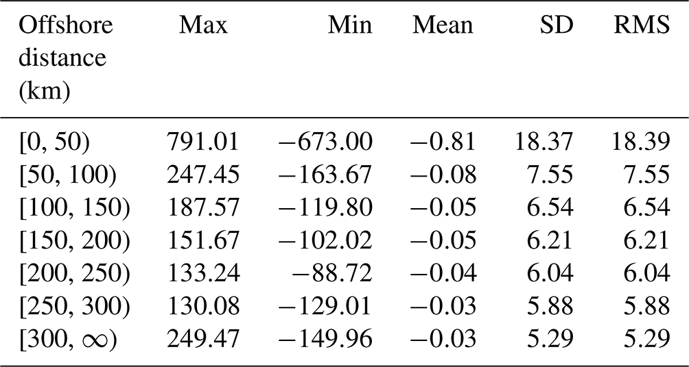
Table 4 Statistical summary of differences obtained by subtracting the SDUSTVGGA model from SIO V32.1 curv at different ocean depths (in E).

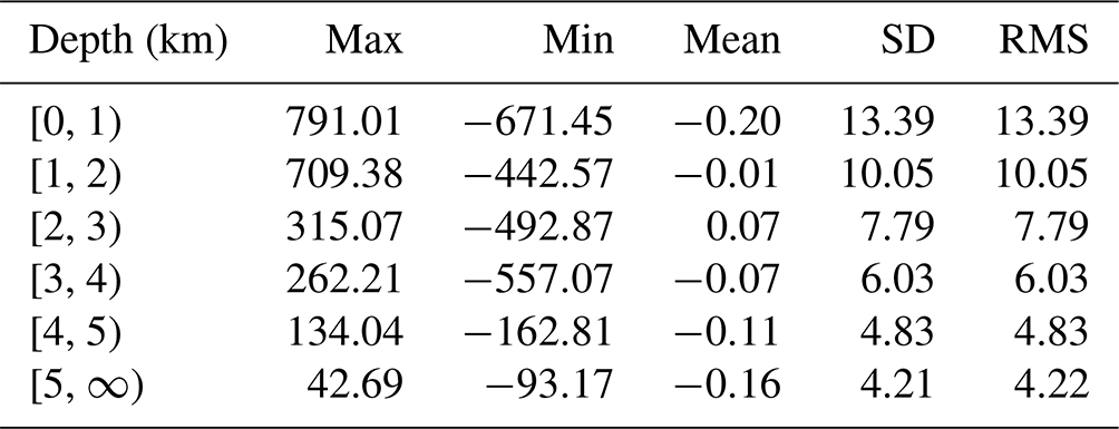
Table 5 Statistical summary of differences obtained by subtracting the SDUSTVGGA model from SIO V32.1 curv at different latitudes (in E).

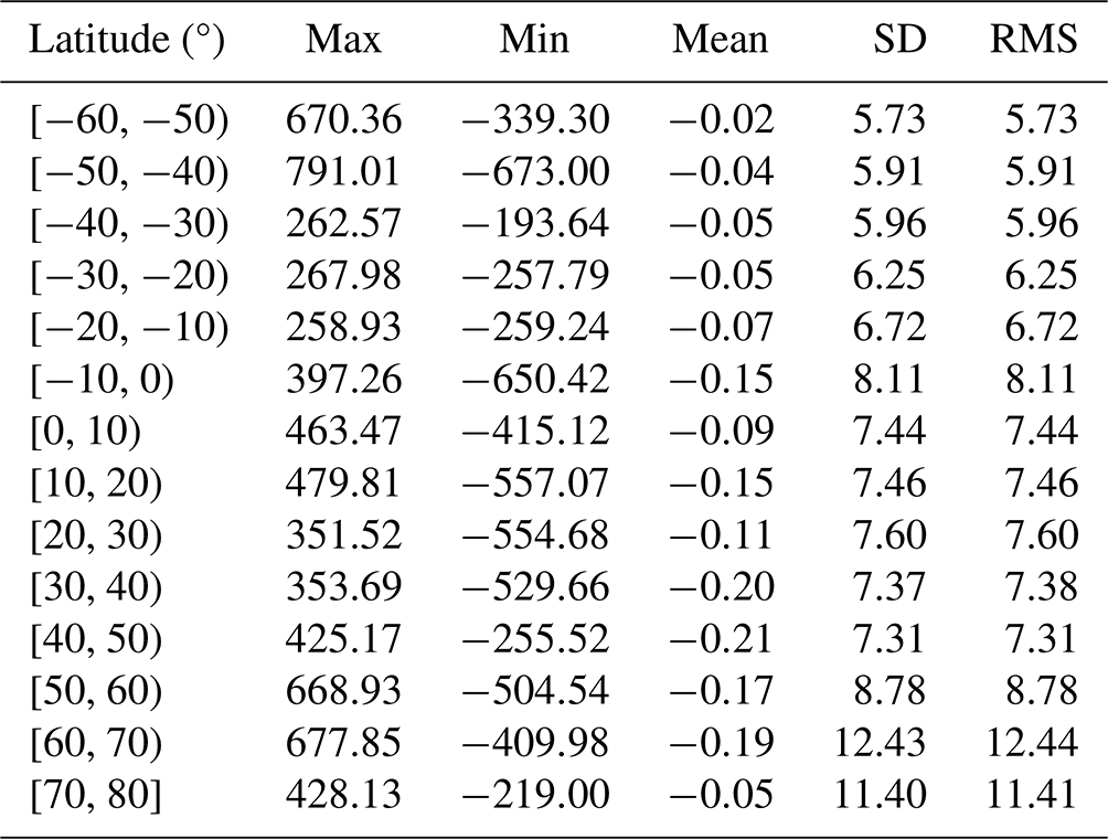
Table 6 Statistical summary of differences obtained by subtracting the SDUSTVGGA model from SIO V32.1 curv at different seafloor slopes (in E).

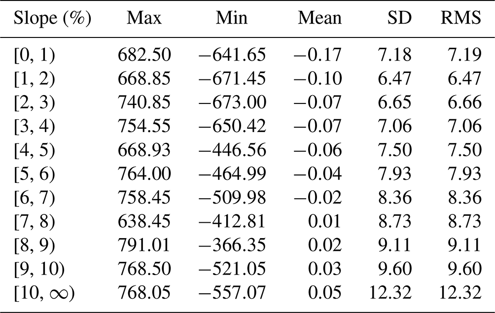
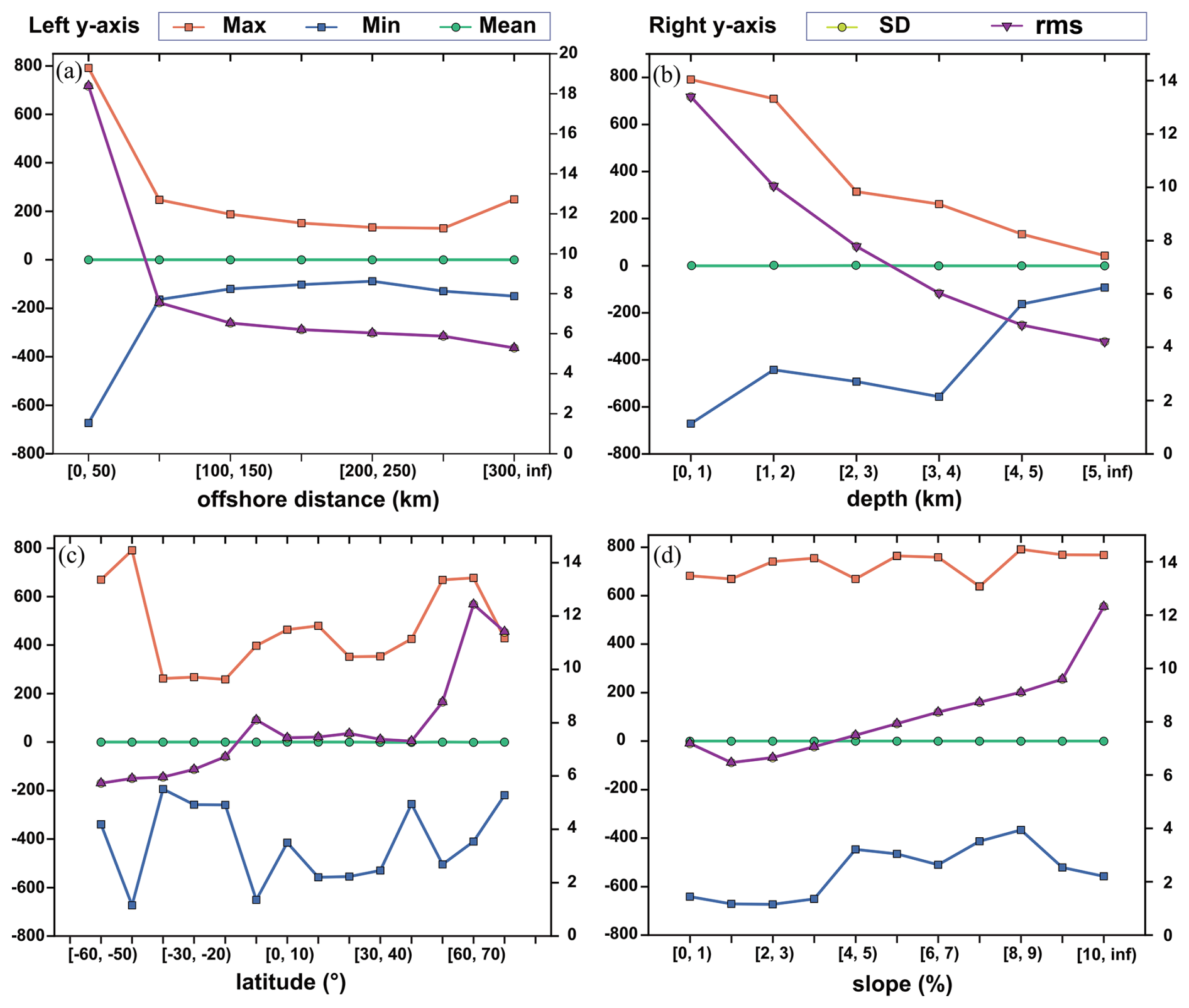
Figure 8 Residuals obtained by subtracting the SDUSTVGGA model from the SIO V32.1 curv model, categorized by (a) offshore distance (km), (b) seafloor slope (%), (c) sea depth (m), and (d) latitude (°). The left y axis represents the max, min, and mean residuals (in E), while the right y axis represents the SD and RMS of the residuals (in E). Note: SD and RMS curves overlap, appearing as a single line.

Table 3 illustrates the impact of offshore distance on the inversion results. As the distance from the coastline increases, the SD of the residual model consistently decreases. Notably, beyond 50 km from the coastline, the reduction in the SD becomes less pronounced. This is likely due to the reduced impact of shallow waters on satellite echo waveforms, which results in less pronounced improvements in data accuracy. In summary, regions closer to the coastline are associated with larger residuals, while deep-sea regions farther from the coast exhibit lower residuals.

Table 4 provides statistical data of residuals across different sea depth intervals. In shallow waters (0–1 km), the residuals show considerable fluctuation, including extreme maximum and minimum values, as well as higher SD and RMS errors. These fluctuations may result from rapid seafloor topography changes in shallow regions, which substantially impact the VGGA calculations. As depth increases, the residuals gradually become smaller and more concentrated, indicating that the model performs more stably and reliably in deep-water areas. This stability can be attributed to the relatively smooth seafloor topography in deeper waters, which introduces fewer interference factors. These results validate that the DTU21 MSS model not only effectively handles oceanic phenomena, such as eddies, but also demonstrates a high level of completeness and robustness in capturing sea surface variability across different ocean environments.

The analysis of Table 5 shows that in the latitude intervals of [−60, −50)°, [−50, −40)°, [−10, 0)°, [60, 70)°, and [70, 80]°, the model exhibits larger extreme values, with maxima reaching 670.36, 791.01, 397.26, 677.85, and 428.13 E, respectively. These high values indicate significant inconsistencies between models in these regions, especially in the high-latitude intervals such as [60, 70)° and [70, 80)°. The SD and RMS values are significantly higher in these intervals, at 12.43 and 11.40 E, respectively, further confirming the greater inconsistencies in high-latitude regions. In contrast, mid- and low-latitude regions exhibit smaller extreme value ranges and lower RMS values, indicating greater model consistency. These results suggest that in mid- and low-latitude regions, the differences between the two models are smaller, indicating overall higher reliability. Considering the orbital inclination of altimetry satellites and their measurement methods, these discrepancies can be attributed to the complexity of geological structures in high-latitude regions. Furthermore, areas near coastlines and shallow waters show greater model differences, increasing the discrepancies between models. The mean values across all latitude intervals approach zero, demonstrating strong global consistency between the two models. This supports the effectiveness of utilizing multidirectional MSS data for global VGGA inversion.

Table 6 examines the impact of seafloor slope on the residual VGGA model. The results show that the SD and RMS values also show an increasing trend with greater slopes. For instance, in regions with slopes less than 1 %, the RMS is relatively low at 7.19 E, indicating higher model stability and consistency. However, in areas where the slope exceeds 10 %, the RMS increases to 12.32 E, suggesting a decrease in model reliability. This observation indicates that as the seafloor becomes steeper, it introduces more sources of interference that challenge the reliability of the VGGA inversion. Additionally, in smoother seafloor regions with slopes under 1 %, the residuals may become more sensitive to noise or systematic errors in the input data, further explaining the slight increase in SD and RMS values observed in these low-slope regions.

To further validate the study's conclusions, five representative regions were selected for model difference analysis. The topographic information of these regions is presented in Fig. 9, providing a comprehensive understanding of the terrain characteristics that may influence model differences.

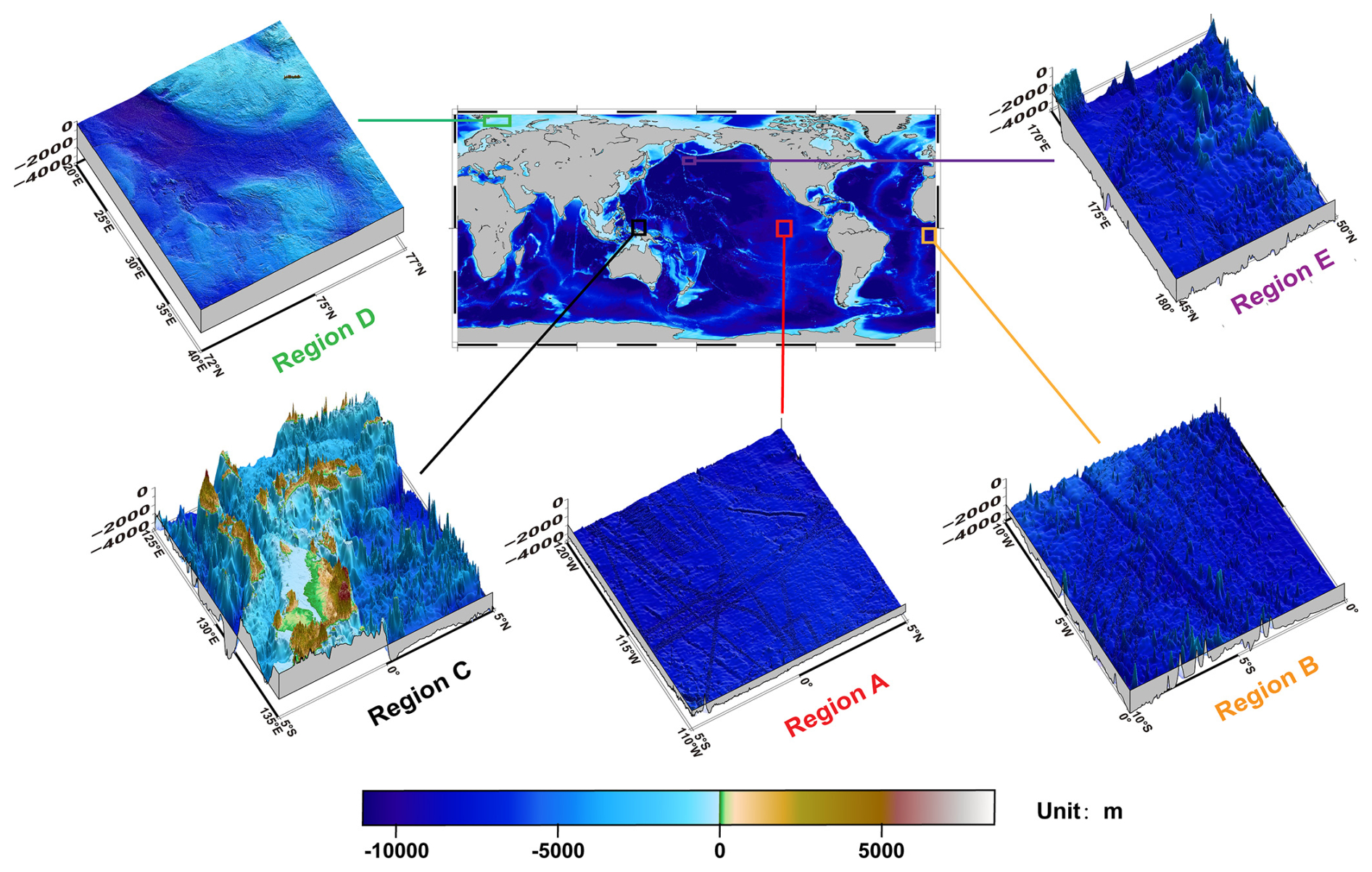
Figure 9 Topographic representation of five selected regions for model difference analysis: (A) the open deep-sea area of the South Pacific far from land, (B) the southeastern Atlantic region near the continental shelf with varied topography, (C) the area near the Indonesian Archipelago with complex seafloor topography, (D) the high-latitude North Atlantic region near the Arctic Circle, and (E) the western Pacific deep-sea region characterized by complex underwater terrain but well-covered by satellites.

The selected regions include the open deep-sea area of the South Pacific far from land (Region A), the southeastern Atlantic region near the continental shelf with varied topography (Region B), the area near the Indonesian Archipelago with complex seafloor topography (Region C), the high-latitude North Atlantic region near the Arctic Circle (Region D), and the western Pacific deep-sea region characterized by complex underwater terrain and good satellite coverage (Region E). A comparative analysis of these regions explored the effects of offshore distance, latitude, and sea depth on the accuracy of altimetry inversion, with statistics provided in Table 7 and modeling results shown in Fig. 10.

Table 7 Statistical comparison of differences obtained by subtracting the SDUSTVGGA model from the SIO V32.1 curv model in different regions (in E).

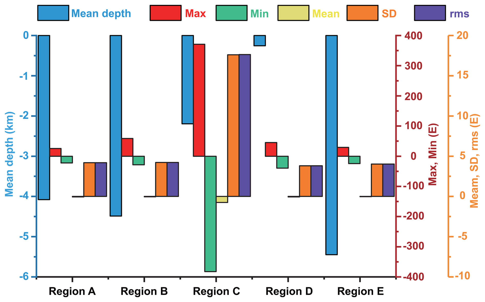
Figure 10 Comparison of differences between the SDUSTVGGA model and the SIO V32.1 curv model across selected regions. The regions include (A) a deep-sea area in the South Pacific, (B) a southeastern Atlantic region with varied topography, (C) the Indonesian Archipelago with complex seafloor features, (D) the high-latitude North Atlantic near the Arctic Circle, and (E) a western Pacific deep-sea area. The bars represent key metrics such as mean depth, maximum and minimum differences, mean, SD, and RMS of the residuals.

Region A in the South Pacific (5° S to 5° N, 120 to 110° W) is located in a remote, open deep-sea area far from any landmasses or islands. The seafloor topography in this region is predominantly flat, with no significant seamounts or trenches. These conditions create a stable environment for satellite altimetry data inversion, leading to minor residuals between the SDUSTVGGA and SIO V32.1 models. The low SD and RMS indicate strong consistency between the models in this region. This suggests that, in open ocean areas distant from land, the model performs with high accuracy and stability, likely due to the minimal interference from topographical variations and external factors.

In contrast, Region B in southeastern Atlantic (10 to 0° S, 10 to 0° W) features varying seafloor topography with an average depth of approximately −4487 m and is closer to the continental shelf. The seafloor topography is more complex than in Region A. As a result, the residual extremes between the SDUSTVGGA and SIO V32.1 curv models are significantly larger, with maximum and minimum differences of 58.73 and −28.32 E, respectively. This indicates that the increased complexity of the seafloor topography introduces greater challenges in the inversion process, resulting in larger discrepancies between the models. These results suggest that in regions with more intricate terrain, satellite altimetry data quality is affected by topographical complexity, resulting in increased uncertainty and decreased model consistency.

Compared to regions A and B, the significantly higher residuals in Region C (5 to 0° S, 125 to 135° E) indicate that the complexity of the seafloor topography, combined with the multipath effect, poses greater challenges for the DTU21 MSS model in low-latitude areas. The steep slopes and varied elevations associated with seamounts and deep trenches introduce greater variability in gravity anomaly signals, complicating the inversion process and decreasing model consistency. As a result, the large residual extremes observed between the SDUSTVGGA and SIO V32.1 models suggest that satellite altimetry data accuracy in this region is more susceptible to interference from local topographical features. These findings highlight that in low-latitude regions with highly complex terrain structures, the model performance is less reliable compared to relatively flat or less complex regions, as seen in regions A and B.

Region D in the North Atlantic near the Arctic Circle (72 to 77° N, 20 to 40° E) has a relatively smooth seafloor topography with an average shallow depth of approximately −256 m. Despite its high-latitude location, the region lacks significant topographical undulations or complex structures. These flat conditions result in smaller residuals between the SDUSTVGGA and SIO V32.1 models, with maximum and minimum differences of 45.18 and −39.44 E, respectively, and an SD and RMS of 3.81 E. The strong consistency between the models in this region is likely due to stable ocean currents in polar areas and comprehensive satellite coverage.

Region E in the western Pacific deep-sea area (45 to 50° N, 170 to 180° E) is characterized by an extremely deep average depth of about −5446 m. Although the seafloor topography here is relatively complex compared to Region B, Region E benefits from better satellite coverage due to its mid-latitude location. Consequently, the residuals between the SDUSTVGGA and SIO V32.1 models are relatively small, with maximum and minimum differences of 29.37 and −24.31 E, respectively. The SD and RMS are 4.02 E, indicating better model performance in this region compared to Region B.

The comparison of these five regions confirms that the DTU21 MSS model effectively manages complex ocean dynamics in deep-sea and high-latitude areas, including regions near polar ice caps, demonstrating its reliability across global oceanic environments. The results indicate that the consistency between the inversion results and the SIO V32.1 model is not directly correlated with sea depth or latitude. Instead, it is the seafloor topography, particularly in shallow-water regions and areas with complex underwater terrain, that leads to instability in satellite altimetry data, which directly affects the consistency between the two models.

5.2 Comparison with curv_SWOT and insights from GEBCO

This study conducted two exploratory experiments to evaluate the performance and potential applications of the SDUSTVGGA model. The first experiment involved a direct comparison with the curv_SWOT model, while the second experiment utilized GEBCO bathymetric data to explore potential correlations between VGGA and bathymetric features.

The curv_SWOT model, derived from the SWOT (Surface Water and Ocean Topography) satellite mission, represents a significant advancement in oceanographic research. The SWOT satellite provides high-resolution and wide-coverage observations, which are crucial for capturing fine-scale oceanic phenomena such as eddies and internal tides. However, the current dataset spans only 1 year, making it a snapshot of short-term oceanic conditions rather than a representation of long-term stable ocean gravity fields. As a result, the curv_SWOT data may contain signals influenced by transient oceanographic phenomena, which could affect its stability and representativeness as a VGGA reference model. The statistical differences between the SDUSTVGGA and curv_SWOT models are summarized in Table 8.

Table 8 Statistical differences obtained by subtracting the SDUSTVGGA model from the curv_SWOT model (in E).

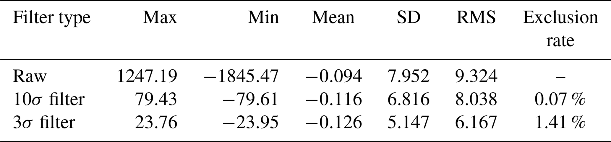
The results in Table 8 reveal significant differences between the SDUSTVGGA and curv_SWOT models. The unfiltered data exhibit a maximum difference of 1247.19 E and a minimum difference of −1845.47 E, with a SD of 7.952 E and a RMS of 9.324 E. These values are notably larger than those observed when comparing SDUSTVGGA with the SIO V32.1 curv model (Table 2), where the maximum and minimum differences were 791.01 and −673.00 E, respectively, with an SD of 7.24 E and an RMS of 8.50 E. This contrast suggests that the curv_SWOT model has a broader dynamic range and higher variability, likely due to its design for capturing fine-scale oceanic phenomena.

Filtering (10σ and 3σ) reduces the differences between the models, as shown in Table 8. However, the broader trends remain consistent with those observed in Table 2. Extreme outliers in the curv_SWOT data, likely associated with transient phenomena such as mesoscale eddies and internal waves, contribute significantly to the observed discrepancies. These transient signals, while valuable for short-term oceanographic studies, differ from the long-term trends captured by the SDUSTVGGA model.

The comparison with the SIO V32.1 curv model further highlights the importance of temporal and spatial characteristics in VGGA modeling. The SIO V32.1 curv model, derived from decades of satellite altimetry data, reflects averaged oceanographic conditions over a long time period. In contrast, the curv_SWOT model's sensitivity to short-term phenomena results in higher variability and a wider dynamic range. This observation explains why the SDUSTVGGA model aligns more closely with the SIO V32.1 curv model in terms of overall variability and dynamic range.

Given the limitations of the curv model and the lack of in situ VGGA measurements, this study further explores the potential of using bathymetric data from GEBCO as an alternative validation approach. However, the indirect and weak relationship between bathymetric features and VGGAs has led to relatively low correlation coefficients and R² values, limiting the strength of the conclusions drawn from this analysis. The analysis results, illustrated in Figs. 11 and 12, highlight these limitations by separately presenting the correlation analysis (Fig. 11) and model performance metrics (Fig. 12). Consequently, these results should be interpreted with caution as the experiment's limitations suggest that the current approach may not fully capture the model's accuracy.

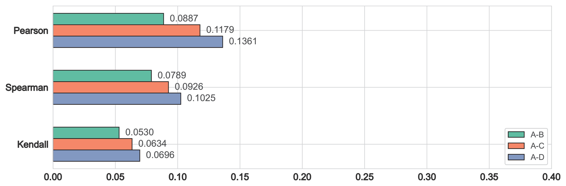
Figure 11 Correlation coefficients (Pearson, Spearman, and Kendall) between the GEBCO bathymetric model (A) and the curv_SWOT model (B), as well as between the GEBCO model (A) and the SIO V32.1 model (C) and the SDUSTVGGA model (D).

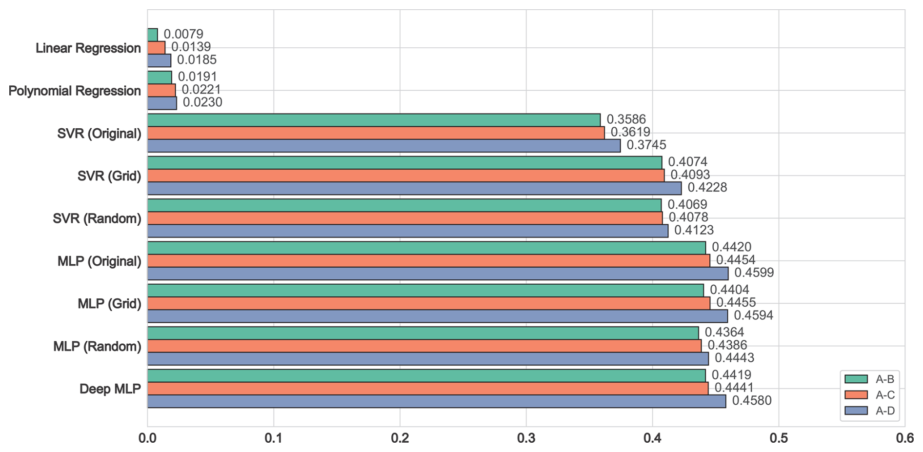
Figure 12 Performance comparisons for regression models applied to GEBCO (A) with curv_SWOT (B), SIO V32.1 (C), and SDUSTVGGA (D). R² values are shown for linear regression, polynomial regression, SVR, and MLP methods, where the MLP used three hidden layers (200, 200, 100 neurons) and deep MLP used seven hidden layers (512, 512, 256, 256, 128, 128, 64 neurons).

The correlation analysis revealed weak positive relationships between the VGGA data (curv_SWOT, SIO V32.1, SDUSTVGGA) and GEBCO bathymetric features. The Pearson correlation coefficients ranged from 0.0887 to 0.1361, with SDUSTVGGA showing the highest value. Similarly, the Spearman rank correlation coefficients and Kendall's τ values also indicated weak monotonic and ordinal associations, further supporting the limited capacity of these models to capture the complex relationships between geophysical processes and bathymetry. These weak correlations may be attributed to inherent differences between bathymetric data and VGGA models as well as potential measurement errors or the complexity of geophysical processes that are not easily captured by these models.

In terms of model performance, regression analysis was conducted using various methods to compare the predictive accuracy of GEBCO with each of the three models. Linear regression models exhibited poor performance, with R² values below 0.02, confirming the inadequacy of simple linear approaches in this context. Polynomial regression models showed slightly better performance, particularly for SDUSTVGGA (R²=0.3586), but still fell short of capturing the full complexity of the relationships.

Nonlinear regression approaches, particularly support vector regression (SVR), provided significantly better results. The original SVR configurations achieved R² values ranging from 0.3586 to 0.3745, with further improvements observed after hyperparameter optimization. The best-performing SVR model achieved an R² value of 0.4228 for SDUSTVGGA, highlighting the value of nonlinear modeling and parameter tuning.

Among the neural network models, the multi-layer perceptron (MLP) with three hidden layers demonstrated the highest performance. The original MLP configuration achieved R² values of up to 0.4599 for SDUSTVGGA, showcasing the ability of neural networks to capture complex nonlinear relationships. Hyperparameter optimization provided marginal improvements, with the MLP (grid) configuration achieving an R² value of 0.4594 for SDUSTVGGA. The deep MLP model, which introduced seven hidden layers, achieved comparable performance, suggesting that additional layers did not lead to overfitting in this case.

It is worth noting that the curv_SWOT model, derived from short-term satellite observations, showed slightly worse performance compared to the other models. This may be attributed to its sensitivity to transient oceanographic phenomena, which are not representative of long-term stable gravity fields. However, the SWOT satellite's high-resolution and wide-coverage capabilities remain valuable for capturing fine-scale oceanic dynamics. These results underscore the effectiveness of neural networks in modeling the relationships between bathymetric data and VGGA models. However, the limitations of using only VGGA data highlight the need for additional data sources or more sophisticated models to achieve more accurate predictions in future studies.

6 Data availability

The DTU21 Mean Sea Surface dataset (Andersen et al., 2023) used in this study is available at https://doi.org/10.11583/DTU.19383221.v1. The CNES-CLS22MDT model (Jousset et al., 2023) can be accessed at https://doi.org/10.22541/essoar.170158328.85804859/v1. The XGM2019e global gravity field model (Zingerle et al., 2020) is available at https://doi.org/10.5880/ICGEM.2019.007. The V32.1 altimetry waveforms dataset (Sandwell et al., 2014; Garcia et al., 2014) can be accessed at https://doi.org/10.1126/science.1258213. The GEBCO_2024 Grid bathymetric data (GEBCO Bathymetric Compilation Group, 2024) is available for download from https://doi.org/10.5285/1c44ce99-0a0d-5f4f-e063-7086abc0ea0f. For calculations in this study, we utilized the ICGEM service (Ince et al., 2019), accessible at https://icgem.gfz-potsdam.de/tom_longtime (ICGEM, 2025). The SDUST2023VGGA model, which includes global ocean VGGA in NetCDF format, is available on the Zenodo repository at https://doi.org/10.5281/zenodo.14177000 (Zhou et al., 2024).

7 Conclusions

This study introduces the SDUST2023VGGA, a global VGGA model derived from the DTU21 MSS model combined with multidirectional MSS data. The model provides a detailed view of VGGA variations over the global ocean and has been rigorously evaluated against the SIO V32.1 model to ensure its reliability. The results show a global residual mean of −0.08 E (Eötvös) and an RMS of 8.50 E, demonstrating the consistency and accuracy of the SDUST2023VGGA model on a global scale.

To construct the model, the global oceanic area was divided into multiple sub-regions to address computational limitations. The geoid was derived by subtracting the CNES-CLS22 MDT influence from DTU21 MSS data, and the remove–restore method was applied to eliminate long-wavelength signals. A weighted least-squares method was used to compute the residual VGGA, which was then combined with the long-wavelength signals to produce the final VGGA model for each sub-region. These sub-regional models were merged to form the SDUST2023VGGA model, covering the latitude range from 80° S to 80° N.

Validation against the SIO V32.1 model revealed strong global consistency. In open ocean basins with relatively flat terrain, the models showed close agreement, while regions near steep seafloor slopes, complex coastlines, and high latitudes displayed larger discrepancies. These differences highlight the challenges of processing altimetry data in complex regions and the influence of topography on VGGA modeling. Analysis of five selected sub-regions (A–E) confirmed that the model's consistency with SIO V32.1 is closely linked to topographical features, validating the robustness of the DTU21 MSS model in addressing complex oceanic and high-latitude conditions.

Two exploratory experiments were conducted to further assess the SDUST2023VGGA model. The first experiment compared the model with the curv_SWOT dataset, revealing significant differences due to the latter's sensitivity to transient oceanographic phenomena. The second experiment explored correlations between VGGA and GEBCO bathymetric data, showing weak relationships but improved performance when using nonlinear methods such as SVR and shallow MLP. These results highlight the challenges of using short-term datasets and indirect validation approaches, emphasizing the need for cautious interpretation.

The SDUST2023VGGA model offers a new approach to studying global VGGA, providing improved coverage and reduced uncertainties in long-wavelength geoid estimation. It shows potential for broad applications in geophysical and oceanographic research, particularly in capturing detailed gravity variations across diverse oceanic regions. The model is openly available, encouraging its use in scientific studies and supporting further validation and refinement.