High resolution continuous flow analysis impurity data from the Mount Brown South ice core, East Antarctica

The Mount Brown South ice core (MBS 69.111° S 86.312° E) is a new, high resolution ice core drilled in coastal East Antarctica. With mean annual accumulation estimated to be ∼ 30 cm ice equivalent throughout the length of the core (∼ 290 m), MBS represents a high resolution archive of ice core data spanning 1137 years (873–2008 CE), from an area previously underrepresented by high resolution ice core data.

Here, we present a high-resolution dataset of chemistry and impurities obtained via continuous flow analysis (CFA). The dataset consists of meltwater electrolytic conductivity, sodium (Na⁺), ammonium (NH${}_{\mathrm{4}}^{+}$), hydrogen peroxide (H₂O₂), and insoluble microparticle measurements. The data are presented in three datasets: as a 1 mm depth resolution record, 3 cm averaged record, and decadal average record. The 1 mm record represents an oversampling of the true resolution, as due to smoothing effects the actual resolution is closer to 3 cm for some species. Therefore, the 3 cm resolution dataset is considered to be the minimum true resolution given the system setup. We also describe the current Copenhagen CFA system, and provide a detailed assessment of data quality, precision, and functional resolution.

The 1 mm averaged, 3 cm averaged, and MBS2023 decadal averaged datasets are available at the Australian Antarctic Data Center: https://doi.org/10.26179/9tke-0s16 (Harlan et al., 2024).

1 Introduction

Ice cores represent some of the best archives available for reconstructing past atmospheric composition, in terms of atmospheric gases as well as atmospheric aerosols. While atmospheric gases are contained and preserved in air bubbles in the ice, aerosols can be preserved as soluble and/or insoluble compounds deposited by dry deposition onto the snow surface or with the snow as wet deposition, and incorporated into the ice matrix as the snow is compressed into ice (Legrand and Mayewski, 1997). The chemical compounds from such aerosols can be measured in the ice itself, either by the chemical composition of the ice (ionic species), or by measuring the insoluble particulate material in the ice.

Many of the aerosol impurities contained in ice cores reflect seasonal variability of aerosol species. However, reconstructing seasonal cycles requires sampling resolution high enough for the seasonal signal to be resolved. This can present measurement challenges, as discrete measurements of trace chemistry of ice samples can require intensive manual decontamination of sampling, which is time consuming and can be difficult to achieve under cold laboratory conditions. Decontamination is especially labor intensive when centimeter-scale measurements are required for ice cores that range from hundreds to thousands of meters in length. Continuous flow analysis (CFA) chemistry measurements, pioneered by Sigg et al. (1994), allow entire lengths of ice core to be sampled continuously in high resolution with very minimal sample decontamination required (Bigler et al., 2011; Kaufmann et al., 2008; Erhardt et al., 2022).

The new Mount Brown South ice core array (MBS), one of the few millennial length ice cores in coastal East Antarctica, represents an important new paleoclimate record from an under-represented region in Antarctica (Vance et al., 2016, 2024a). The full length of the MBS main core has been dated and the chronology (MBS2023, used here) is described in Vance et al. (2024a).

CFA chemistry and impurity datasets provide high-resolution continuous records that can be useful for reconstructing climatic variability of the region (Kjær et al., 2022; Erhardt et al., 2023). Additionally, CFA conductivity and microparticle records can provide useful in distinguishing potential volcanic eruption signals in the record (Abbott et al., 2024). Seasonally varying chemistry species, including sodium and hydrogen peroxide can be useful in annual layer counting and chronology refinement (Vance et al., 2024a). Discretely measured data from the upper (satellite-era) sections of the four MBS ice cores have been used to investigate an East Antarctic proxy for El Niño variability (Crockart et al., 2021), as well as to understand precipitation climatology effects on the water-isotope record for the coastal East Antarctic site (Jackson et al., 2023). We suggest that, among other uses, a high resolution CFA dataset from MBS is well suited to expand on studies of such large modes of climate variability.

Here we present the high-resolution, CFA record of chemistry and insoluble impurity measurements for the full length of the MBS Main ice core. The data set is presented alongside a description of the analytical system and methodology, as well as considerations about data quality and uncertainties in both the concentration and the depth/temporal resolution of the record.

1.1 Mount Brown South

Four ice cores were drilled during the 2017–2018 austral summer field season at the coastal East Antarctic Mount Brown South site (MBS1718-Main, -Alpha, -Bravo, and -Charlie). Here we present CFA data for the MBS1718-Main core only.

1.1.1 Ice core site

The Main core drill site lies at 69.111° S, 86.312° E, 2084 meters ASL (Fig. 1), adjacent to the boundary between Princess Elizabeth and Wilhelm II Land, approximately 62 km south of the Mount Brown nunatak, and located 12.6 km WSW of a short surface core drilled in December 1998 (known as “MBS99”, Smith et al. (2002); Foster et al. (2006)). The three MBS shallow cores (Alpha, Bravo, and Charlie), were drilled nearby (within 100 m of the main core site) to depths of 20.41, 20.225, and 25.86 m, respectively, but data from these cores are not included in this dataset.

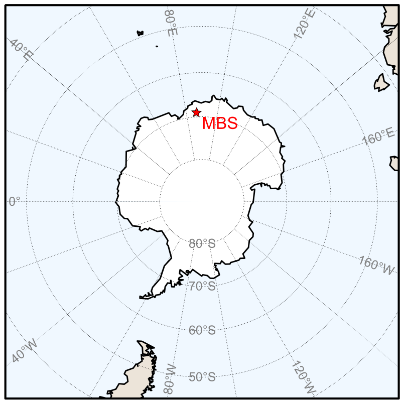
Figure 1 Map showing the location of the Mount Brown South site.

While the four cores drilled during the 2017–2018 season are named MBS1718, for simplicity, we refer to them here as simply MBS. The MBS site was selected based on six criteria as described in Vance et al. (2016) in order to (1) preserve a millennial-scale record in the 300 m archive; (2) undergo minimum snowmelt in summer; (3) preserve sub-annual resolution (minimum accumulation of 25 cm yr⁻¹ ice equivalent (IE)); (4) experience minimal surface reworking; (5) have undergone minimal ice advection at 300 m depth; and (6) add novel information to the existing network of East Antarctic ice cores. Average accumulation at the site is found to be 30 cm IE per year over the satellite era (1978 to 2017, based on annual layer depth counting of the shallow cores) (Crockart et al., 2021) and the site is characterized by wet deposition (Crockart et al., 2021; Vance et al., 2024a). Mean annual surface air temperature at the MBS site is −29.7 °C (based on the Modèle Atmosphérique Régional (MAR) regional climate model, Agosta et al., 2019), and the site is characterized by predominantly easterly prevailing winds (Vance et al., 2024a). Drill site characteristics for the MBS site are presented in Vance et al. (2024a) and detailed climatology of the site is well described by Jackson et al. (2023) and Crockart et al. (2021).

Vance et al. (2024a) presents the MBS2023 chronology, a combined depth-age scale for MBS-Main and MBS-Charlie. The main core covers 1137 years (873–2008 CE), while the three co-located surface cores (Alpha, Bravo, and Charlie) cover approximately the satellite era through to drilling year (2017–2018).

1.1.2 MBS chronology

An age scale has been developed for the MBS ice cores, described thoroughly in Vance et al. (2024a). The ice core dating and layer counting was based on a combination of stable water isotopes (Gkinis et al., 2024) and discrete chemistry measurements. Discrete trace ion measurements were performed using ion chromatography (IC) on ∼ 3 cm samples, using a Thermo-Fisher/Dionex ICS3000 ion chromatograph (for a more detailed description of the discrete impurity measurement methods, see Crockart et al. (2021) and references therein). Chronology development relied primarily the ratio of sulfate to chloride, and there was found to be significant variability in annual layer thickness throughout the length of the core. The chronology was determined by two independent layer counting efforts, one relying on volcanic matching, the other primarily relying on variable chemistry species. These two efforts were followed by careful consideration and joint determination of uncertain years (Vance et al., 2024a). Development of the MBS2023 chronology did not rely on the CFA impurity record, and the CFA dataset presented here is analytically independent from the discrete dataset and chronology presented in Vance et al. (2024b). We encourage direct users of the MBS CFA dataset to use the MBS2023 chronology (Vance et al., 2024b), or any subsequent updates thereafter.

1.1.3 Sample description

The MBS cores were drilled as part of a joint Australian-Danish collaboration. The MBS main core was drilled from a depth of 4.25 m (depth at the top of the borehole, accounting for the recessed floor of the drilling tent and drill trench) to 294.79 m depth using the Danish Hans Tausen ice core drill (9.8 cm core diameter). The ice was transported from the drill site to Hobart, where it was described (in terms of core quality, including breaks, cracks, and other damage to the core), logged, and imaged in the −18 °C freezer laboratories at the Institute for Marine and Antarctic Studies. There, it was sectioned lengthwise for analyses. An interior piece with 34 × 34 mm cross section area along the entire length of core was designated for CFA chemistry (Fig. 2). See Vance et al. (2024a) for a full description of the ice processing.

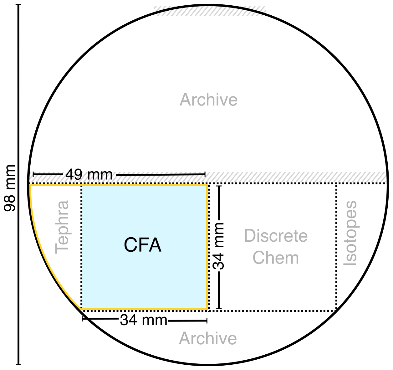
Figure 2 Schematic diagram showing the cross-section of the MBS main core, with sample sections shown. Dotted lines indicate cuts made with a bandsaw. Shaded area (hatched line) indicates surfaces planed for intermediate layer core scanning. Section shipped to Copenhagen shown outlined in yellow, with CFA stick shaded in blue.

The CFA section, still attached to the wedge-shaped outer edge piece designated for tephra sampling, was transported to Copenhagen, where the samples were prepared for CFA by removing said outer wedge at freezer facilities at the Physics for Ice, Climate and Earth (PICE) at the Niels Bohr Institute (NBI). To minimize potential contamination, the horizontal ends of each sample piece, including any breaks occurring within a sample, were carefully cleaned by scraping with a ceramic blade immediately prior to being placed in frames for melting on the Copenhagen CFA. Approximately 1–2 mm of ice was removed from each break in the ice in this cleaning process. All sample pieces were measured both before and after cleaning, and any ice removed in cleaning has been accounted for in the depth record.

1.2 Continuous flow analysis

CFA is particularly well suited for measuring trace chemical species and impurities at high resolution (millimeter to centimeter scale) for long ice cores (Sigg et al., 1994; Bigler et al., 2011; Erhardt et al., 2022). This allows for the production of seasonal-scale records of aerosol species spanning thousands of years at sites with sufficiently high accumulation. CFA is advantageous compared to discrete methods such as ion chromatography, as it provides the ability to analyze ice core samples at speeds of up to four centimeters per minute and with minimal time required for decontamination and sample changeover (Röthlisberger et al., 2000; Kaufmann et al., 2008; Erhardt et al., 2023).

The CFA process involves melting a vertical section of an ice core (typically from top to bottom) by placing it on a purpose-built heated plate (melthead) connected to a melt water extraction system. The melthead used in the Copenhagen CFA system is designed to prevent contamination, such that the external portion of the core section is diverted to waste and thus manual decontamination is only required along the horizontal surfaces at core breaks (Bigler et al., 2011). The inner decontaminated melt water is debubbled and subsequently diverted through a system of measurement instrumentation using a series of peristaltic pumps. Measurements are taken continuously, with data recorded each second (Kaufmann et al., 2008). The detectors used are chosen for their short response time and ability to detect the low impurity concentrations observed in polar ice (Sigg et al., 1994; Röthlisberger et al., 2000).

The modular nature of CFA allows it to be simplified for deployment to the field for in-situ measurements (Kjær et al., 2021). It may also be expanded for additional gas (Stowasser et al., 2012; Rhodes et al., 2013) and isotope (Gkinis et al., 2011; Jones et al., 2017) measurements in addition to chemistry and impurities (Bigler et al., 2011). The Copenhagen CFA setups used in the 2018 and 2019 MBS campaigns both build on the CFA setup described in Bigler et al. (2011) and Kjær et al. (2022). Both campaigns used the same system components, however, the entire CFA system was relocated to a new building between campaigns. The move resulted in some differences between the setups, which are detailed below.

The chemistry and impurity measurements from both campaigns include insoluble microparticles (dust > 1 µm), electrolytic conductivity, calcium (Ca²⁺), sodium (Na⁺), ammonium (NH${}_{\mathrm{4}}^{+}$), hydrogen peroxide (H₂O₂), and meltwater acidity. Additionally, sulfate (SO${}_{\mathrm{4}}^{\mathrm{2}-}$) was analysed in 2018. The acidity, sulfate, and calcium records, however, are not presented here, due to independent problems with the measurement systems for those species.

2 MBS continuous flow analysis

The basic setup of the Copenhagen CFA system is well described in Bigler et al. (2011) and Kjær et al. (2022), and is based on previous CFA systems such as Kaufmann et al. (2008) and Röthlisberger et al. (2000). The CFA measurements took place over two sampling campaigns. The dry-drilled section (∼ 5–95 m depth) of the main core, and the Charlie core (25.86 m) were analyzed in 2018. The remaining (wet-drilled) section of the main core (∼ 95–295 m depth) was analyzed in 2019 after the CFA laboratory was relocated to another building. Flow diagrams for the two systems used for the MBS CFA measurements can be seen in Fig. 3. Details of adaptations to the system made between the two campaigns are described below.

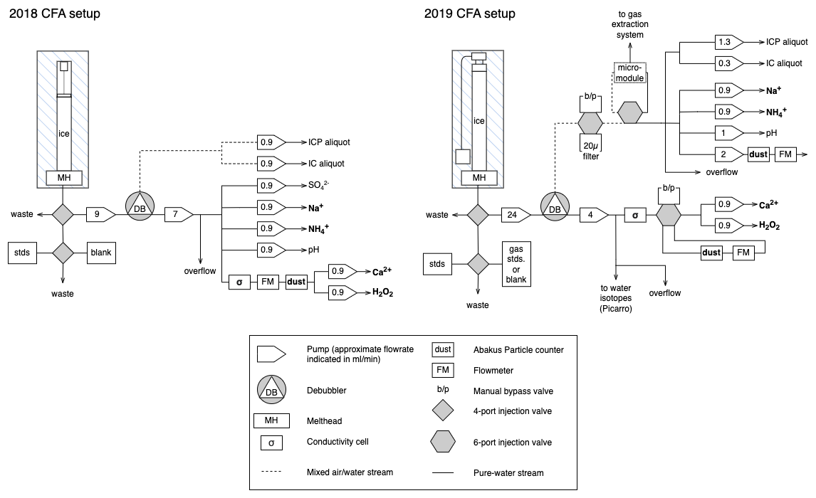
Figure 3 Schematic flow diagram of the CFA systems used for the 2018 and 2019 measurement campaigns at the Physics of Ice, Climate, and Earth in Copenhagen.

The CFA base functionalities are very similar between the two analytical campaigns: sticks of firn/ice are placed into polycarbonate frames for mounting above the melter system consisting of the heated melthead (Bigler et al., 2011) and above it a short ice alignment guide (∼ 20 cm), all held inside a freestanding freezer unit maintained at approximately −20 °C. The frames and alignment guide allow for each new stick of ice to be added to the system before the previous stick is fully melted. This allows for continuous melting of multiple (typically 5–10) meters of ice during each run similar to the CFA procedure described in Erhardt et al. (2023) and Kjær et al. (2022).

As the ice is melted, meltwater from the clean interior of the sample is pumped to the analytical systems using peristaltic pumps (ISMATEC), while water from the potentially contaminated outer ice is diverted to waste. Both setups employ the use of an enclosed debubbler consisting of a flat triangular cell to remove air bubbles from the sample stream (Bigler et al., 2011). Both systems utilize a commercially available conductivity meter to measure meltwater electrolytic conductivity, as well as an Abakus laser particle counter (LDS23/25bs; Klotz GmbH, Germany) coupled with a flowmeter to determine the number of insoluble particles larger than 1 µm mL⁻¹ of sample volume (Simonsen et al., 2018). Simple fluorescence or absorption spectroscopic methods are used to determine NH${}_{\mathrm{4}}^{+}$, Ca²⁺, H₂O₂, Na⁺, SO${}_{\mathrm{4}}^{\mathrm{2}-}$, and meltwater acidity, using instrumentation and methods specifically designed for CFA (Kaufmann et al., 2008; Sigg et al., 1994; Röthlisberger et al., 2000; Erhardt et al., 2022; Kjær et al., 2022, 2016). Reagents and buffers for analysis were prepared weekly or bi-weekly as required with respect to their rate of deterioration. Additionally, during both campaigns, aliquots were collected in vials for later analysis using ion chromatography (IC) and inductively coupled plasma mass spectrometry (ICP-MS), the results of which are not included in this dataset and will be released in a future publication.

2.1 Specifics for the 2018 CFA setup

The 2018 CFA measurements took place at the Center for Ice and Climate at the University of Copenhagen in the laboratory described also by Simonsen et al. (2019) (which at that point was located at Juliane Maries Vej Copenhagen) during October-November 2018.

An optical depth registration system (Waycon LLD-150-R5232-50H) was used for registration of the melt speed during the 2018 campaign, in a setup similar to that used in Dallmayr et al. (2016). While the laser distance meter allows for precise melt speed and sample length measurements (± 2 mm accuracy, and 0.5 mm resolution), it can be temperamental as vibrations from ambient activity (heavy footfalls or accidental knocking of the freezer enclosure) can disrupt measurements. Additionally, the ice is never a perfect fit to the frame and as it melts it changes from leaning on one side of the frame to the next causing some additional noise seen in the very precise laser measurement. Additionally, the space required for the laser system limits the length of the frames used in the freezer, thus limiting the sample stick length to 50 cm. For the campaign in 2018, 10 sample sticks (5 m) were melted continuously per run, book-ended by standards runs (see Sect. 4.3 and Table A1 in the Appendix).

A sulfate measurement system following the method used for NorthGRIP (Kaufmann et al., 2008; Erhardt et al., 2022) was trialed in the 2018 system, but due to a high limit of detection of the system, sulfate measurements were unsuccessful, and thus are not presented here. Discrete sulfate measurements of the full MBS record via ion chromatography can be found in Vance et al. (2024a).

2.2 Specifics for the 2019 CFA setup

In October–November 2019 the Physics of Ice, Climate, and Earth at the University of Copenhagen moved to a new address at Tagensvej 16. Due to the relocation the 2018 system was dismantled and rebuilt in the new location. During reassembly changes were made to the system, described herein.

A cable-driven rotary encoder (draw wire position transducer, SX80, WayCon; sensitivity: γ = 25 counts mm⁻¹, linearity: ± 0.15 %) was implemented for depth registration in 2019 similar to that described in Bigler et al. (2011). This encoder setup freed up more space in the freezer unit, allowing for melting of meter long sample sticks and thus the data from the 2019 campaign has fewer sample breaks per run as 5–10 samples (5–10 m) were melted continuously per run. Further, all chemistry lines were optimized in length to minimize dispersion and thus smoothing of the final record.

As part of the 2019 rebuild, a gas extraction system (3M, Liqui-Cel MM-0.75 × 1 Series) coupled to the mixed air-water stream from the top of the debubbler unit was added to the CFA. While the gas extraction system was not used for data collection during the MBS melting campaign, it was sporadically implemented for testing and refinement throughout the 2019 measurements. Further detail on the gas extraction system and its impact on measurement quality follows in Sect. 5.1 below.

2.3 Primary differences between 2018 and 2019 CFA setups

As described above, the two system setups used in the MBS CFA measurements are largely similar, using much of the same equipment and instrumentation. The primary differences, and their potential impact on measurements between the two setups are as follows.

• Depth registration system: The 2018 setup utilized a laser distance meter reflecting off of a weight placed on top of the ice, while the 2019 setup used a cable-driven rotary encoder attached to a weight resting on the top of the ice. Additionally, the two instruments result in different amounts of “downtime” in the system during ice stick frame changeover, with slightly more time required when changing frames with the rotary encoder system. While these factors might influence the resulting CFA depth scale, these offsets can be cross-checked with the lengths measured in the freezer during sample preparation. These differences are minimal, and likely within the scope of the measurement error of the instrumentation.

• Ice stick length: The ice core was cut into approximately one meter long pieces in the field, for shipping and storage. Due to differences in depth registration instrumentation (the laser distance meter takes up substantially more vertical height than the draw-wire encoder in the limited freezer height), for the 2018 melting the CFA sticks were cut into approximately half-meter long ice sticks, while the full ∼ 100 cm long sticks were used in 2019. The ∼ 50 cm ice sticks introduce additional breaks in the ice which may introduce more potential contamination than with the ∼ 100 cm ice sticks. However, the ∼ 50 cm ice sticks have the advantage of allowing increased certainty of absolute depths, as the lab-measured top depths are known every ∼ 50 cm.

• Melt rate: The ice melt rate was slightly different for the two setups. The impact of the melt rate on sample smoothing and resolution is discussed further in Sect. 4.1.

• Gas extraction system and stable water isotope measurement: The 2019 setup introduced both a gas extraction system and an in-line cavity ring-down spectrometer (Picarro L-2140i) for stable water isotope measurements. The gas extraction system is described in more detail in Sect. 5.1, and the stable water isotope measurements are described in Gkinis et al. (2024). As the gas extraction system required a higher sample volume, the pumped flow rates through the system was different between the two setups (see approximate flow rates in Fig. 3). This resulted in more overflow routed to waste per minute of melting in the 2018 setup than in the 2019 setup. Notably, the target flowrate through each individual measurement instrument is similar for both systems (e.g. ∼ 1 mL min⁻¹ for each chemistry line and ∼ 2 mL min⁻¹ for the conductivity and dust measurement lines; target flowrates for each analyte are presented in Fig. 3).

3 Data processing

3.1 Depth scale

Precise depth information is crucial for ice core data. The position-derived melt rate data collected during CFA campaigns is used to reconstruct the total length of ice melted, to which the recorded length of ice removed during preparation must be re-introduced at the appropriate depths. To account for the time when the encoder is removed during the frame changes, for both the laser and draw-wire encoder, the position data is used to identify the times just before and after each frame change period, and the average melt rate over the previous period of uninterrupted melting is used to reconstruct a continuous melt rate. The down-time that occurs during frame changeover is slightly longer for the draw-wire encoder than that of the laser encoder, as the draw-wire assembly that is attached to the encoder must be fully removed from the remaining ice and subsequently replaced once the new frame has been mounted.

The information recorded during sample preparation is used (including ice removed for decontamination at sample ends and breaks and poor-quality ice not analyzed), together with the position of each break as logged during melting, to create appropriately sized gaps in the depth scale corresponding to the missing ice. The depth scale is finalized by assigning the top of each CFA data run to the recorded top depth of the corresponding bag from the accepted field depth measurements. Manual decontamination of the cores can introduce slight (sub-millimeter) discrepancies due to mis-reading lengths on the standard ruler used in preparation as well as slight misjudgments and biases in identification of break positions during melting. These unavoidable inaccuracies are estimated to be on the scale of one or two millimeters at most.

In rare cases, measured lengths of the same stick varied from one measurement to another (for example, when measured in Hobart prior to shipping to Copenhagen). This was found to be due to slightly slanted cuts where one core meets the next, with one measurement taken from the long side and another taken from the short side. These discrepancies were found to amount to less than 0.01 % of the length of the record (Gkinis et al., 2024). Careful consultation of comprehensive line scan images of the core sections was used to correct for these errors and determine the most accurate core length across all measurements. This process required the depth scale for the entire Main core to be developed, taking into account small differences in field to lab core lengths as well as any small discrepancies in the IC (discrete chemistry) stick lengths. This is described in detail in Vance et al. (2024a). Any such differences were accounted for in the development of the CFA depth scale in the precise assignment of the top depths at approximately every meter. This top depth assignment was done to prevent any small discrepancies from propagating through the length of the core. Additional description of the depth scale procedures can be found in Gkinis et al. (2024).

3.2 Calibrations

The absorption and fluorescence spectrometric methods used for chemistry concentration measurements require calibration to convert from instrument signal voltage/light intensity to concentration. In order to properly calibrate these instruments, standard solutions with predetermined chemical concentrations are passed through the system before and after each sample run. A multi-element standard solution is used for a three step calibration of the Ca²⁺, Na⁺, and NH${}_{\mathrm{4}}^{+}$ measurements (Merck Certipur^® IC Multi-element Standard VII). A single component standard solution is used for a two step calibration of H₂O₂ (Sigma-Aldrich Hydrogen Peroxide Solution 30 wt % in H₂O). The multi-element standard solutions are prepared prior to each run, and the peroxide standards are prepared prior to each run from a first dilution prepared at the start of each measurement day. All standards are prepared using ultra-pure deionized water (Merck RiOs™ 16 Milli-Q^®). Standard recipes and resulting concentrations are presented in Table A1.

Calibrations are calculated from the standards, which were run at the beginning and end of each measurement run, as described in Kaufmann et al. (2008) and Erhardt et al. (2023). This allows for monitoring of system drift and provides ample standards data for each run, in case any issues arise during a standards run. Each standard solution is passed through the system in series and the resulting signal voltage was recorded both manually and by the LabVIEW software used to operate the system. For the fluorescence method (Ca²⁺, NH${}_{\mathrm{4}}^{+}$, and H₂O₂ measurements), the standard calibration is based on the linear relationship between concentration and fluorescence signal voltage. Sodium is a pseudo-absorption method, and calibration is based on a curve fit to the standard signal response (Kaufmann et al., 2008). Calibrations are computed using a semi-automated script written in MATLAB. The script isolates the signal voltage at each standard input concentration and calculates the appropriate calibration coefficients. The standards are well fitted, with the average r² value for the calibration curves for each analyte being greater than 0.99.

3.3 Signal delay time

Due to differing distances of each of the measurement instruments from the melter, there is a time delay between when the ice passes the melter and when the measurement takes place.

The time delay between the ice on melter and when the measurement is recorded down stream is calculated in two parts. Firstly, there is the elapsed time from when the sample parcel passes the melter to when it is divided into disparate melt streams for each analytical unit. The bulk melt delay time is measured during sample melting as the elapsed time from when the first sample ice passes the melter (recorded as observed by lab operator) and the initial peak response observed in the conductivity measurements. Conductivity is used as it is located closest to the melter (by tubing distance/mixing volume as well as time), and thus the first signal to respond. In both systems, the approximate total time offset between the sample ice reaching the melter and the response seen in the conductivity signal was approximately 40 s.

Secondly, there is a delay time individual to each species measured due to the internal dynamics of each analytical melt stream. These response delay calculations are computed based on each instrument response time during the standards runs. This additional delay time is measured as the time elapsed between when the signal increase is seen in the conductivity measurements and target species. We determined that additional delay time as time at which the derivative of the response curve of each standard reaches a maximum (approximating the midpoint of the signal response rise). The average delay time (from all standards runs used in calibration) is presented in Table 1.

Delay times vary for each species, but are similar between the two system setups (Table 1). Other choices for delay calculations could have been to use the start or end of the signal rise. However, due to smoothing, these points can be hard to reliably identify, whereas the maximum of the derivative of the increase is easily and systematically identified. However, we recognize that this can introduce a minor offset between methods that are highly smoothed in comparison to those that have faster response times.

Table 1 Average delay time in seconds for each analyte measured as elapsed time between conductivity signal response and analyte signal response, based on the maximum of the first derivative of the signal response measured during each standards run.

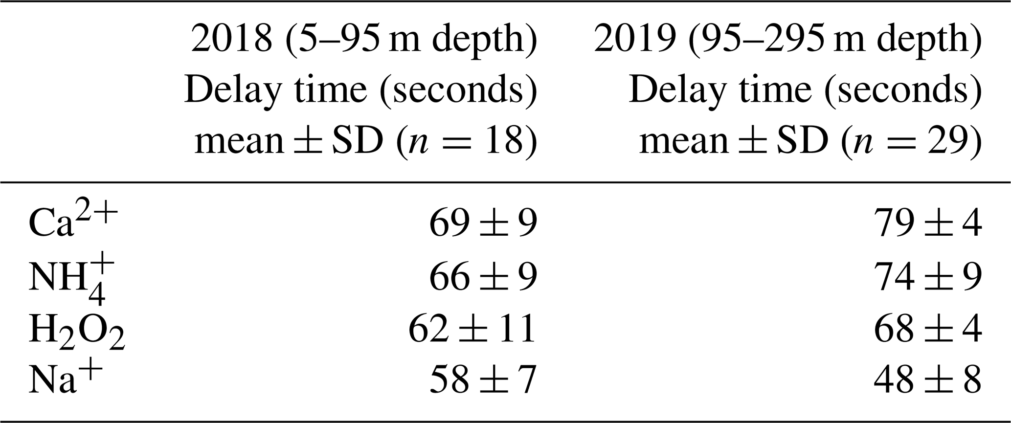
As the delay times can vary slightly from run to run, due to factors including tubing length, tubing wear, and fluctuations in melt speed, delay times for each species were measured and applied individually to each CFA run of 5–10 m of ice melted. Each delay time estimation was calculated based on the standards data collected either immediately prior to or following the run.

3.4 Calcium data

Expected concentrations of calcium at the MBS site are very low (median chemistry concentration from the discrete chemistry measurements is 0.142 ppb). Due to the nature of the system, and the limits of the ultrapure water system used to produce the standards, reagents, and baseline values for measurements produced here, this is significantly below the limit of detection we are reliably able to achieve using the Copenhagen CFA system (see Table 2). As the CFA Ca²⁺ data for MBS does not show any discernible seasonal cycles throughout the record, and the calibrated Ca²⁺ concentration values measured close to or below the LOD of our instrumentation, we consider these values too low to report.

Table 2 Sample data range, median, and LOD for all measured species, and standard deviation (SD) of lowest-concentration standard for each chemistry analyte.

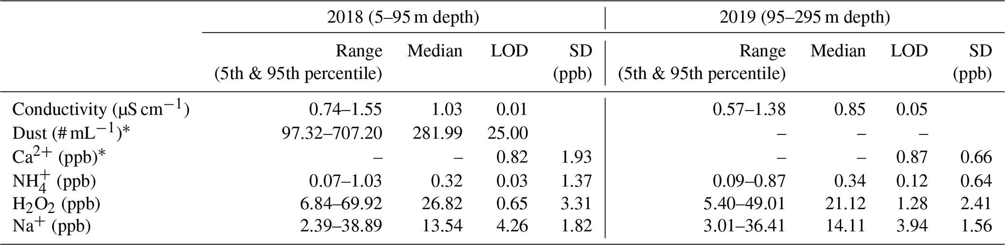
^*Dashes indicate data not included in the published dataset.

4 Data resolution and smoothing

4.1 Sampling resolution

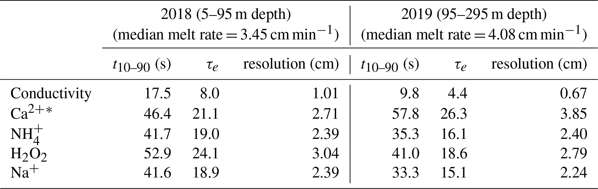
Data is registered at one second time steps, and thus the sampling resolution varies with melt rate. The melt rate of the CFA system is selected to optimize resolution, while accounting for density changes from firn to ice, however with the introduction of the gas extraction system in 2019, the melt rate was calibrated to produce optimal gas volumes for simultaneous measurement. The 2018 CFA setup operated with a target melt rate of ∼ 4.5 cm min⁻¹ throughout the upper 35 m depth, decreasing across 10 m to reach ∼ 3 cm min⁻¹ below 45 m depth (median actual melt rate 3.45 cm min⁻¹ across the full 2018 record). The 2019 campaign (∼ 95–295 m depth) had a target melt rate of 4 cm min⁻¹ (median actual melt rate 4.08 cm min⁻¹). These median melt rates produce a direct sampling resolution (independent of smoothing due to response time) of 0.58 and 0.68 mm, respectively.

4.2 Signal dispersion smoothing

The internal dynamics of the system (mixing volumes and flow conditions within tubing) lead to signal dispersion, as described by Breton et al. (2012). This gives a smoothing effect, wherein a discrete parcel of sample is measured in the CFA system as a dispersed signal spread across a short time period (on the order of a few seconds) spanning the expected signal response time for that parcel (Breton et al., 2012). This dispersion time is calculated as as an e-folding time based on the 10 %–90 % rise time in the signal response during the standards run. Based on the melt rate, it is possible to use this dispersion signal time to calculate the effective smoothing length (and thus a minimum realistic resolution) for each species (Table 3). Although the melt rate used in 2019 was faster than in 2018 (4.08 and 3.45 cm min⁻¹ respectively), the shorter response times (due to shorter tubing lengths used in the rebuilt system) resulted in a higher resolution in 2019.

It is worth noting that, as described by Breton et al. (2012), the signal peak under realized (dispersed) flow conditions occurs slightly before the expected signal response under idealized “plug flow” conditions. This effect is linked to the specific dynamics of each CFA system, and similar to Erhardt et al. (2022), we do not quantify this slight offset for the Copenhagen system, but note that it could lead to a slight systematic offset (on the order of a few millimeters) biased towards shallower sample depths.

Table 3 Response time as 10 %–90 % rise time (t_10–90) and e-folding time (τ_e) and resultant effective smoothing length based on melt rate (resolution). Values shown for each of the two system setups from 2018 and 2019 (and the depths measured during each campaign).

^* Data not included in the published dataset.

5 Uncertainties and limitations

5.1 Gas extraction system interference

During the 2019 CFA melting campaign, the introduction of a new gas extraction system was trialed. This system setup comprised a gas extraction line originating from the upper outlet of the debubbler, coupled to a micro-module which extracts dry air from the sample stream for gas analysis. These system trials influenced the internal pressure balance of the chemistry system tubing. This had a significant impact on the meltwater acidity (pH) measurements (Kjær et al., 2016), which suffered from back pressure changes influencing the sensitive dye to water ratios, making the pH record unusable. The gas extraction system also impacted the insoluble microparticle data collected by the ABAKUS laser particle counter.

While the specifics of the gas extraction system are beyond the scope of this data description, there is a visible signature in the microparticle record that only occurs when the gas extraction system was on-line with the chemistry CFA. The signature can be seen as a significantly elevated baseline in the microparticle record (measured from Milli-Q^® ultrapure water through the system), as well as an alteration in the amplitude of the dust signal. These changes correspond with the recorded valve switches of the gas system. Due to the nature of the system interference, we are not able to reliably correct for this interference. We therefore only present the insoluble microparticle data measured in 2018 before the gas system testing began. Due to additional concerns with data quality and contamination of the microparticle record in the deepest portion of the dry drilled section, we only present microparticle data down to 85 m depth.

5.2 Analytical precision

The limit of detection (LOD) varies for each detection channel. Sample concentration ranges, LOD, median, and standard deviation for each of the analytical detection channels are presented in Table 2. LOD is calculated as 3 times the standard deviation of the blank signal measured on ultrapure (Milli-Q®) water during the standards runs (Röthlisberger et al., 2000; Gfeller et al., 2014). The standard deviation (SD) of the lowest concentration standard (9.9 ppb for Ca²⁺, Na⁺, and NH${}_{\mathrm{4}}^{+}$ 60 ppb for H₂O₂) is also used as a measure of precision of the system. Frequency histograms for each measured species are presented in Fig. 4.

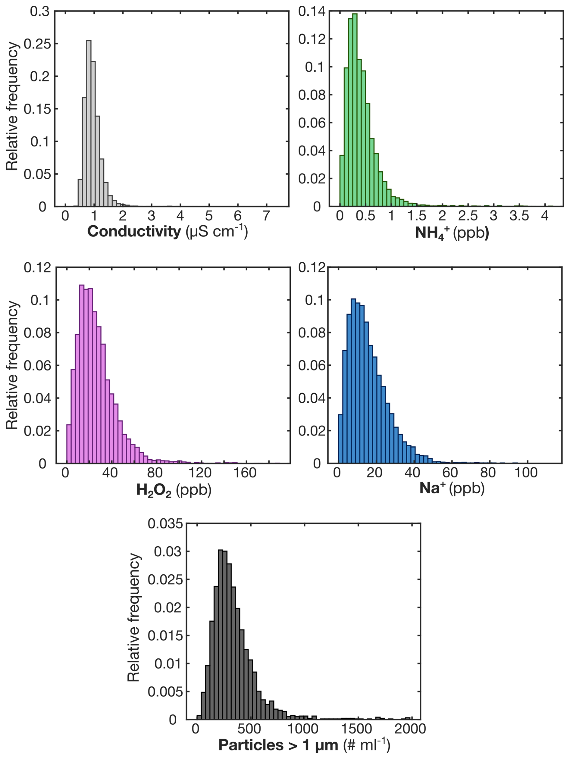
Figure 4 Relative frequency histograms demonstrating the variability of the impurity data (conductivity (µS cm⁻¹), peroxide (H₂O₂, ppb), sodium (Na⁺, ppb), ammonium (NH${}_{\mathrm{4}}^{+}$, ppb), and insoluble microparticles (dust, particles mL⁻¹ > 1 µm)). Histograms computed based on 3 cm averaged resolution dataset. See Fig. A1 in the Appendix for comparison of CFA and discrete sodium datasets.

5.3 Standards preparation

Measurement uncertainty for the wet chemistry analyses is driven primarily by uncertainty in standards preparation, due to instrument uncertainty of the microliter pipette (20–200 µL Socorex Acura manual^®) and bottle-top dispenser (Dispensette^® III 5–50 mL, Brand GmbH). This uncertainty is discussed in Gfeller et al. (2014), and as standards used here were prepared in a similar manner, the uncertainty estimate is less than 10 % (Gfeller et al., 2014; Erhardt et al., 2023).

5.4 Contamination and data cleaning

Despite careful decontamination of the ice samples prior to melting, some cleaning of the data is still necessary. Often, very short-duration, high concentration spikes can be seen in the data signal due to occasional air bubbles passing through the measurement cells in the instruments despite the use of debubbler and gas permeable membranes (Accurel^®) immediately prior to each detector. These particular signals are easily identified and removed from the record by a simple 10 s smoothing, or (as implemented here) by using a filter that applies a threshold cutoff to the differential of the signal (due to the characteristics of these features). The passage of air bubbles through the detectors results in a signal which is characterized by a significantly steeper increase (and subsequent decrease) in the signal voltage than anything produced by variability in the ice core sample. Because of this characteristic peak shape, we are able to define for the differential of the dataset, a threshold, values above which we use to define “bubble spikes” in the data, which can be safely removed from the dataset.

Contamination signals at core breaks, due to contamination from drill fluid (Estisol-140) or general laboratory contamination, are also relatively easily removed (Erhardt et al., 2022). This type of contamination is characterized by a steep increase in particle count followed by an exponential decay as the contaminated sample passes through the system. For this record, the data coinciding with signals deemed to be caused by this type of contamination have been manually removed from the dataset.

Due to the very low concentrations in Antarctic ice of all species measured and the sensitivity of instrumentation, some measurements fall very close to or below the limit of detection of the system. Data that fall below baseline values (measured from Milli-Q^® water run through the system before and after each run) have been removed from the dataset.

6 Data quality assessments

6.1 Conductivity peak matching

To verify data quality and depth scale accuracy, and to demonstrate the ability of the CFA record to correlate with signals identified in the discrete dataset, we investigated all conductivity peaks that fall above 3σ from a 90 cm moving mean of the conductivity record. The 90 cm window was chosen as on average it represents an approximation of 3 years, despite the known accumulation variability shown in the MBS cores. Using this method, we are able to identify 72>3σ conductivity peaks. Of these 72 peaks, 16 correspond with volcanic events reported in Vance et al. (2024a) to within one year age-at-depth uncertainty. Volcanoes identified in this method include Pinatubo (1991), Agung (1963), Tambora (1815), Mount Mélébingóy/Parker Peak (1640), Ruiz (1595), and Samalas (1257), in addition to a number of the unknown peaks identified in MBS (Table A2). This method identifies additional peaks above 3σ, however, these have not been matched to volcanoes identified in Vance et al. (2024a), and may be attributed to factors other than volcanic signals.

We attribute existence of peaks that are not identified in both datasets to the differences in the data types used (comparing conductivity to non-sea salt sulfate) as well as the method of peak identification. Because the peak identification method used here is based solely on bulk conductivity, it is likely that some peaks are related to sources of other soluble ions, in addition to volcanic sulfate. Vance et al. (2024a) use the non-sea salt sulfate, calculated from bulk sulfate following (Plummer et al., 2012), a more specific indicator of volcanic horizons than bulk conductivity, and therefore likely to be better able to distinguish more volcanic horizons. Additionally, Vance et al. (2024a) identified and matched volcanic events qualitatively based on assessment of the size, shape, and relative concentration of sulfate compared to existing Antarctic records (WAIS divide, Law Dome, and Roosevelt Island), while we use a simple cutoff threshold method (3σ above the moving mean), which is likely to miss lower-magnitude volcanic horizons that would be more easily identifiable by their shape rather than simply the maximum peak conductivity.

Due to the marginal location of the MBS site, volcanic signals stand out less from the background conductivity record (as a measure of bulk ions) than those of more inland sites (Winstrup et al., 2019). This is due to the proximity to the coastline and increased influence of oceanic sources of impurities leading to dilution of the signal (Plummer et al., 2012; Winstrup et al., 2019; Vance et al., 2024a). When a total ion budget is considered (based on discrete ions), peaks in the total ions can be seen that are not associated with elevated sulfate (see Fig. A2).

Jackson et al. (2023) use back-trajectory analysis through the satellite-era to demonstrate that meridional transport pathways are disproportionately represented during the extreme precipitation events that influence MBS accumulation. We hypothesize that this meridional transport pathway might also influence impurity transport to MBS. The greater background influx of impurities due to the coastal location is likely to inhibit the ability of the simple threshold cutoff method used here on the conductivity record to `see” all volcanic horizons able to be identified based on volcanic sulfate.

Accounting for the impact of the different methods used, we consider the ability of the CFA conductivity signal to identify half of the volcanic events found in the non-sea salt sulfate signal by Vance et al. (2024a) across the MBS record to be an external validation of the CFA depth scale and conductivity record described here.

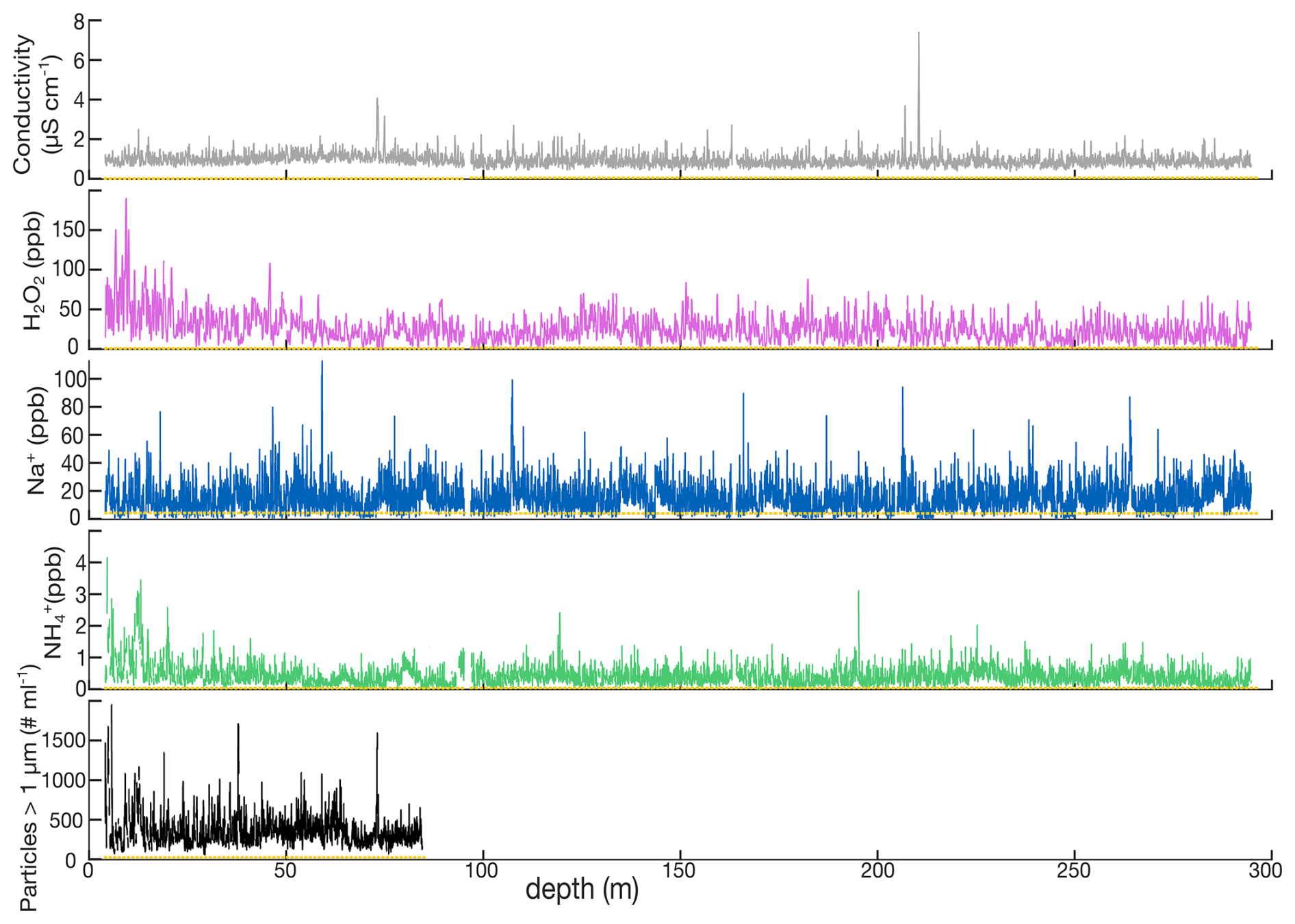
Figure 5 Overview of the full CFA record for MBS at 3 cm resolution. Data include electrolytic conductivity of meltwater (Conductivity, µS cm⁻¹), peroxide (H₂O₂, ppb), sodium (Na⁺, ppb), (d) ammonium (NH${}_{\mathrm{4}}^{+}$, ppb), and (e) insoluble microparticles (dust, particles mL⁻¹ > 1 µm). Dashed yellow line indicates LOD for each analyte (see Table 2). Gaps in the dataset indicate sections where ice was removed for decontamination, lost in processing, or where analytical issues resulted in poor data quality.

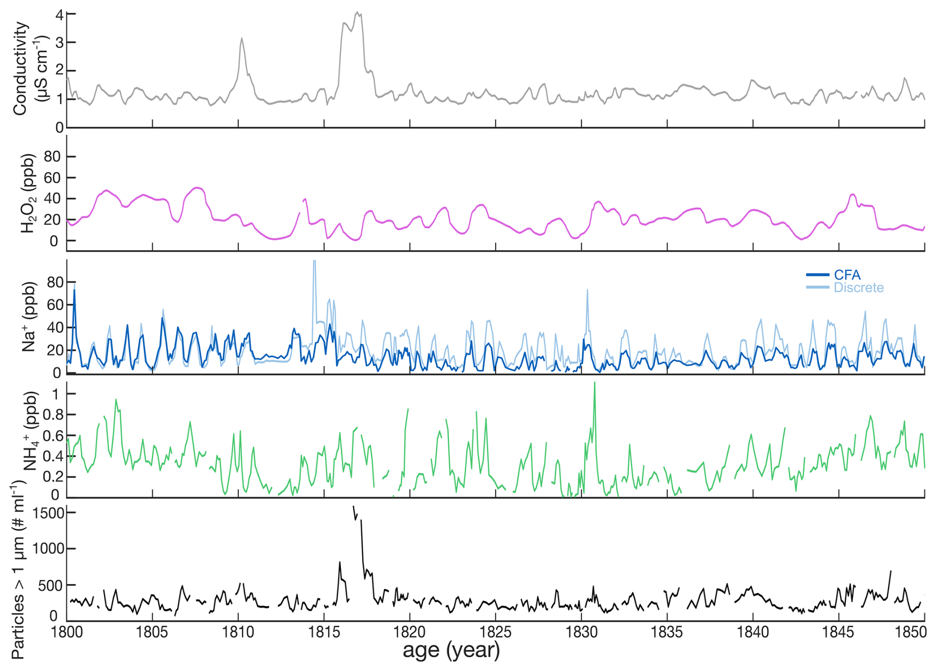
Figure 6 50 year subset of the 3 cm averaged resolution dataset, covering the period from 1800 to 1850 CE, plotted on the MBS2023 chronology (Vance et al., 2024b). Discrete sodium record shown alongside CFA data for comparison purposes. Data shown correspond with the depth range covering approximately 77.55–63.60 m depth of the data presented in Fig. 5. Note the peaks in both conductivity and insoluble microparticles (dust) corresponding with the influence of the 1815 Tambora eruption, one of the volcanic horizons utilized in the development of the MBS2023 chronology (see Fig. A2).

6.2 Comparison to discrete dataset

Because discrete measurements have been performed on the full MBS-Main core (Vance et al., 2024b), we are able to use the discrete record as a comparison dataset to investigate similarities and/or differences in the datasets. The only species measured directly with both methods is sodium, which we use here to cross-check the reliability of our methods and data quality. The published discrete datasets (Vance et al., 2024b) present the raw IC data with minimal data quality assessment beyond the satellite-era section (top ∼ 20 m) of the main core presented in Crockart et al. (2021). As such, there appear to be some outlier samples, likely due to lab contamination, however, a quality assessment of the discrete dataset is beyond the scope of this work. The discrete IC data were measured in micro-equivalents per liter (µeq L⁻¹), and have therefore been converted to ppb for comparison to the CFA dataset presented here. In order to produce a direct comparison of the two datasets, the data were resampled (using a simple linear interpolation method) to a common depth scale at 3 cm resolution.

On visual inspection, the two datasets appear to be very well correlated. The seasonal variability of the Na⁺ signal can be clearly identified and peaks can be easily matched between the two datasets. Slight deviations in magnitude can likely be attributed to the differences in measurement method used (ion chromatography vs. fluorescence detection). The CFA method for measuring sodium ions relies on complicated chemical reactions including a reaction column which must be regularly recharged (Kaufmann et al., 2008), and thus minimal drift in the signal is expected. While there are also slight discernible depth discrepancies between the two records, these discrepancies are minor (on the order of a few mm) and do not propagate significantly throughout the record. The discrete Na⁺ dataset is included for visual comparison in Fig. 6 as well as Fig. A1. It can be seen in the histogram comparison of the dataset that the measured concentration ranges are similar, however with a somewhat higher median concentration measured in the CFA dataset. To assess variability between the two datasets, we have compared the records using Pearson's correlation, and the two datasets show a significant, but moderate to weak correlation (r=0.4307, p>0.001).

While an inter-lab comparison across these two methods is helpful, it is important to note that issues such as contamination and measurement error are not inherently more likely in one method than the other. Discrepancies between the two datasets, therefore, do not necessarily indicate problems with the CFA dataset presented here. Regardless, the significance of the correlation between the datasets, both in the measured concentration ranges (Fig. A1) and the alignment with depth (Fig. 6), do provide validation and reassurance with regards to the quality of the measurements presented here.

7 Dataset description

We present the CFA records in three formats. First, we present the data at 1 mm resolution (full dataset averaged to 1 mm using the CFA depth registration). Although this is in reality an oversampling of the data with regards to the smoothing inherent in the system, we consider this the full dataset at a minimum resolution allowing reduction of instrument noise. While this over-samples the true resolution when accounting for signal smoothing, the 1 mm resolution dataset can be helpful in identifying extreme events in the dataset which may be artificially smoothed by the moving mean method used to produce the 3 cm averaged dataset.

We also present the data on 3 cm resolution (3 cm averaged), which is above the effective resolution of the instrument-smoothed data for the majority of the measured species. The 3 cm resolution dataset is lower resolution than the “true” smoothed resolution of most of the CFA analytes (all except for peroxide above ∼ 95 m and calcium below ∼ 95 m). However, we chose this resolution so as to provide a cohesive and user-friendly dataset with all species on the same depth scale, despite the fact that this under-represents the resolution of higher-resolution species like conductivity. Additionally, due to the large annual layer thickness throughout the full record (0.3 m IE yr⁻¹ mean accumulation) and minimal layer thinning expected at this site (for the 295 m core bottom depth with a bedrock depth of approximately 2000 m; Vance et al., 2016), data resolution of 3 cm is able to resolve sub-annual features throughout, as seen also in the 3 cm discrete samples (Crockart et al., 2021; Vance et al., 2024a). Figure 5 shows the full length of the CFA record on 3 cm resolution, while Fig. 6 highlights a 50-year subset of the data to demonstrate the resolution of the 3 cm averaged dataset, plotted on the MBS2023 chronology (Vance et al., 2024b). Finally, for ease of use in climate reconstruction application, we present the record as a decadal-scale (10-year) record. The decadal scale record is computed as a 10-year running mean. This is based on the MBS2023 chronology presented in Vance et al., 2024a), and any future changes in the MBS chronology will not be reflected in this dataset.

Due to the characteristics of accumulation/deposition at the MBS site, care should be taken with interpretation of sub-annual features produced from the 1 mm and 3 cm datasets. We refer readers to Jackson et al. (2023) for a discussion of the impacts of the intermittent precipitation and accumulation variability of the site, and Crockart et al. (2021) for satellite-era climatology and precipitation estimates.

The datasets presented here (Harlan et al., 2024) have been cleaned and corrected, both manually and through automated processes. Despite these extensive quality control methods, we cannot guarantee the absence of any spurious data or false signals arising from measurement error or lab contamination.

8 Data availability

The datasets described here (1 mm averaged, 3 cm averaged, and decadal averages on the MBS2023 age scale) are available for download from the Australian Antarctic Data Centre (AADC) https://doi.org/10.26179/9tke-0s16 (Harlan et al., 2024).

9 Code availability

The MATLAB script described here, used in calibration of the CFA dataset, is available as a Supplement with this manuscript.

10 Conclusions

Here we present a high-resolution chemistry and impurity record from the MBS ice core (MBS1718). We present records of electrolytic conductivity, insoluble microparticles (dust), calcium (Ca²⁺), ammonium (NH${}_{\mathrm{4}}^{+}$), sodium (Na⁺), and hydrogen peroxide (H₂O₂). Based on the chronology presented in Vance et al. (2024a), this record spans 1137 years (873–2009 CE). The data set described here represents the highest resolution chemistry record of the full length of the MBS ice core. We are pleased to make this dataset available for public use with considerations to the above comments on resolution and data quality, and the authors remain available for questions by end users.

Appendix A

Table A1 Recipes used in standard solutions. Standard (Std) concentrations used are shown in bold.

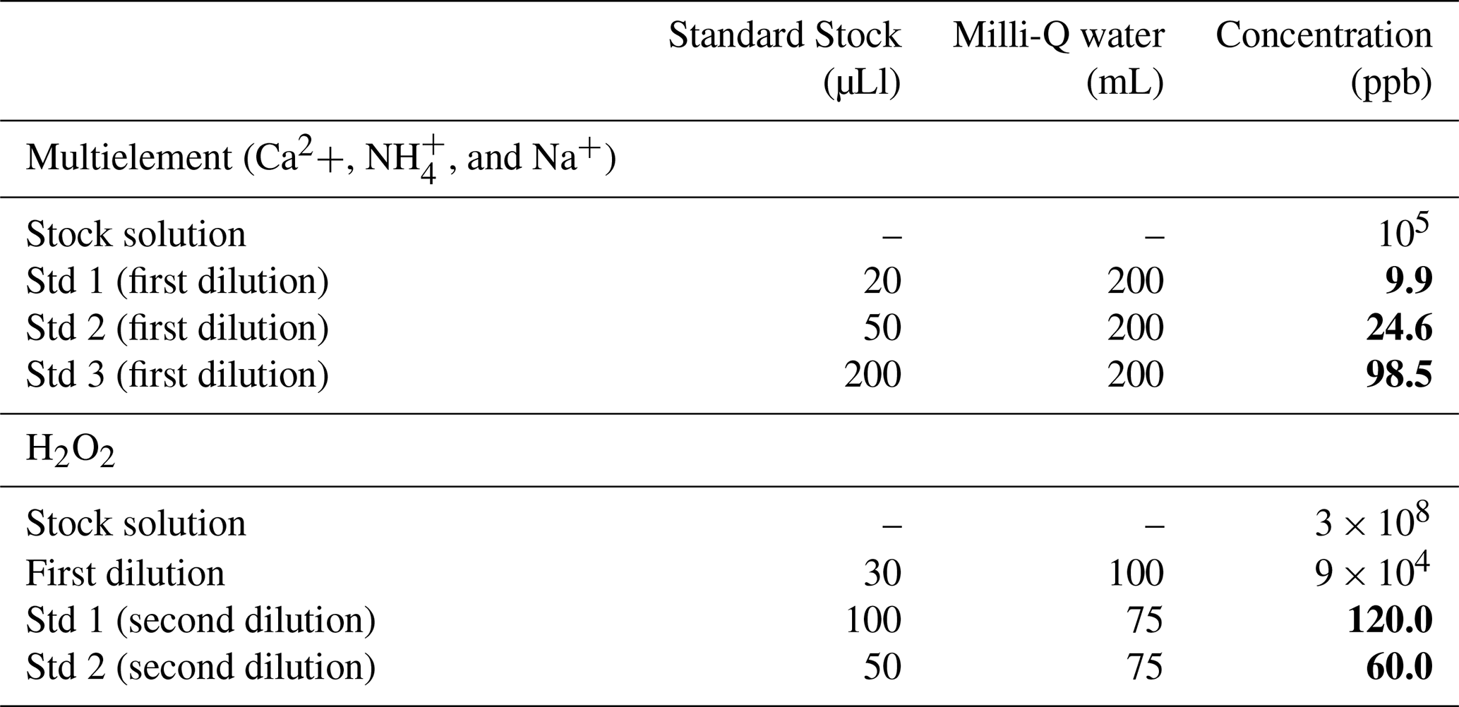
Table A2 Proposed eruption events seen in MBS from Vance et al. (2024a). Events matched with CFA conductivity peaks identified as more than 3σ above the 3 year mean. Vance et al. (2024a) depths identified using estimation of the non-sea-salt component of the sulfate from the discrete ion chromatography measurements performed at the Institute for Marine and Antarctic Studies in Hobart, Tasmania, Australia. Dates provided are the volcanic horizons used in development of the MBS2023 chronology (Vance et al., 2024b).

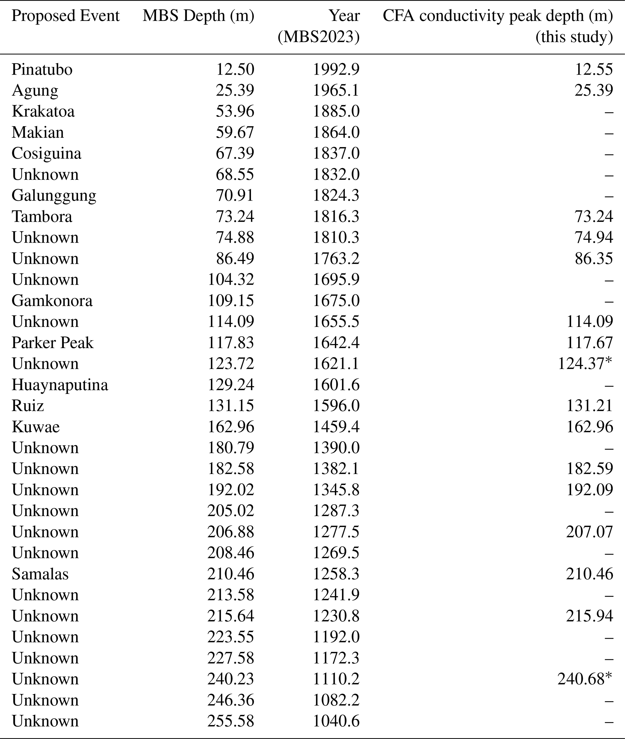
^* Conductivity peaks with depths close to identified eruption depths in MBS, but not within 30 cm (∼ 1 year).

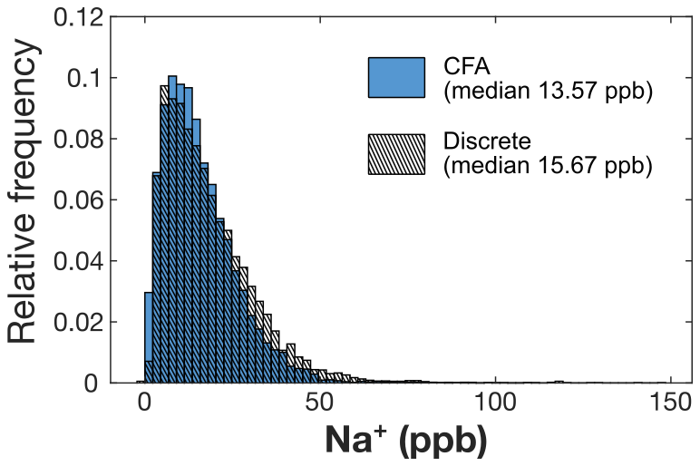
Figure A1 Relative frequency histograms and median value (in ppb) comparing the CFA (blue bars) and discrete (hatched bars) measurements of sodium (Na⁺, ppb). Histogram and median value calculated from 3 cm resolution data for the full record of both CFA and discrete datasets.

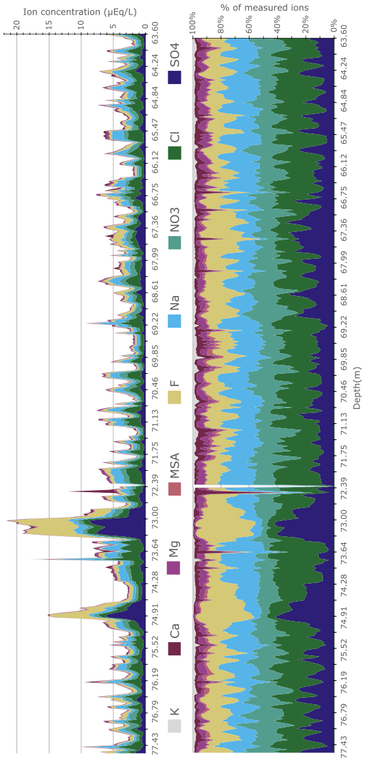
Figure A2 Total discrete measured ions in MBS-Main by depth, shown as concentration (µEq L⁻¹) and relative abundance (% of total ions measured). Ions measured by ion chromatography, from 3 cm resolution discrete samples Vance et al. (2024b). Depth range corresponds approximately to that shown in Fig. 6 in main text (approximately 1800–1850).