Generation of global 1 km daily land surface–air temperature difference and sensible heat flux products from 2000 to 2020

Accurate estimation of land surface sensible heat flux (H) is crucial for comprehending the dynamics of surface energy transfer and the cycles of water and carbon. Yet, existing H products mainly are meteorological reanalysis datasets with coarse spatial resolutions and high uncertainties. FLUXCOM is the sole remotely sensed product with its 0.0833° spatial and 8- temporal resolution spanning from 2001 to 2015, so there is still a need for accurate and high spatial resolution global product based on satellite data. To address these issues, we generated the first global high resolution (1 km) daily H product from 2000 to 2020 using long short-term memory (LSTM) deep learning models, incorporating data from the Global LAnd Surface Satellite (GLASS) product suite. Furthermore, considering that the difference between land surface temperature and air temperature (Ts-a) is a key driver of H, we introduce the first global accurate satellite-based Ts-a product. This product refines the uncertainty compared with obtaining Ts-a directly from existing products by subtracting air temperature from land surface temperature. Our model, distinct from previous models that estimate H per pixel through physically-based models requiring parameters that are not readily accessible, can conveniently derive global values and efficiently capture nonlinear interactions. Additionally, it accounts for the temporal variation of H. Validation against independent in-situ measurements yielded a root mean square error (RMSE), mean absolute error (MAE), and coefficient of determination (R²) of 25.54 W m⁻², 18.649 W m⁻², and 0.54 for H, and 1.46 K, 1.073 K, and 0.52 for Ts-a, respectively. The estimated H and Ts-a values are more accurate than current products such as MERRA2, ERA5-Land, ERA5, and FLUXCOM under most conditions. Additionally, the new H product offers more detailed spatial information in diverse landscapes. The estimated global average land surface H from 2000 to 2020 is 35.29±0.71 W m⁻². These high-resolution H and Ts-a products are invaluable for climatic researches and numerous other applications. The daily mean values for the first three days of each year can be freely downloaded from https://doi.org/10.5281/zenodo.14986255 (Liang et al., 2025a), and the complete product is freely available at https://www.glass.hku.hk/ (last access: 8 September 2025).

1 Introduction

Sensible heat flux (H) is the turbulent transfer of heat between the land surface and the atmosphere, primarily driven by temperature differences (T₀–T_a, also referred to Ts-a, where T₀ (K) represents the surface aerodynamic temperature and T_a (K) the air temperature) (Mito et al., 2012). As a major energy source for the lower atmosphere and a critical component of surface energy fluxes, H plays a vital role in land-atmosphere interactions, particularly in thermal exchanges between the land surface and the atmospheric boundary layer (Beamesderfer et al., 2023; Liao et al., 2019). The uneven distribution of H leads to alternating absorption or release of heat into the atmosphere, affecting monsoon circulation and local climate systems (Mito et al., 2012; Zhou and Huang, 2014; Zhou and Huang, 2010). Therefore, accurate estimation of H is essential for studying global energy flows and understanding the dynamic transfers of water, energy, and trace gases at the Earth's surface (Watts et al., 2000).

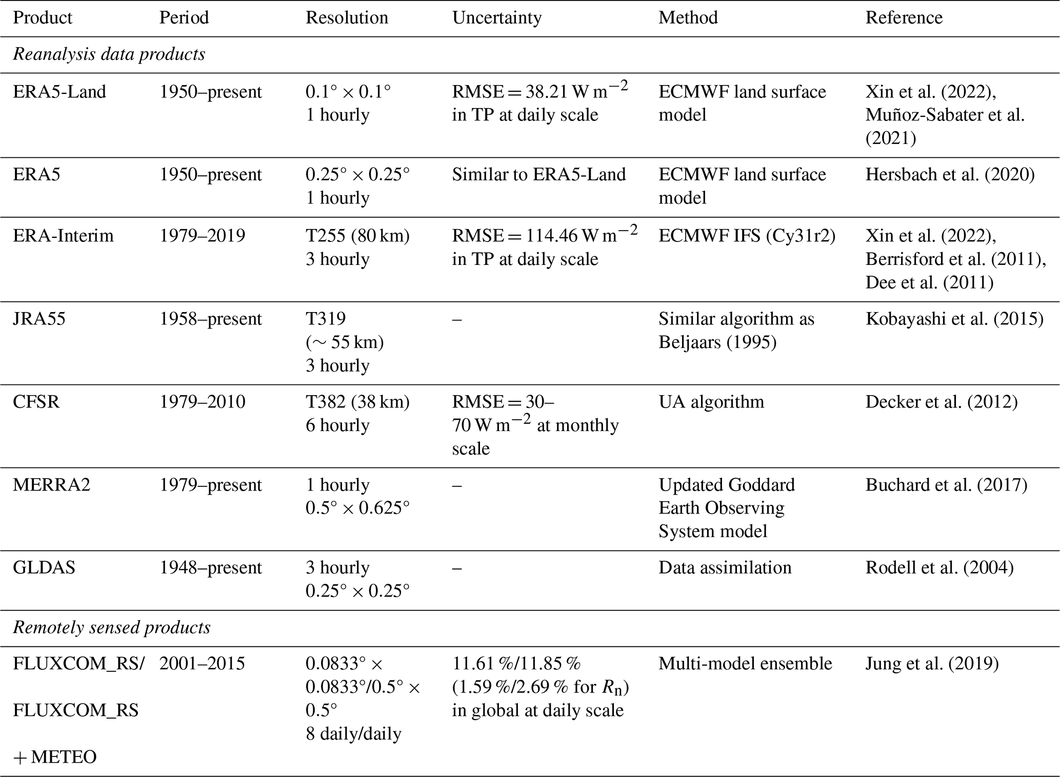
Currently, H can be derived from ground-based measurements or various products. Ground measurements, considered as “ground truth” values, are typically obtained using eddy covariance (EC) system (on the scale of hundreds of meters) and large aperture scintillometer (LAS, at the kilometer scale). The EC system measures instantaneous variations in vertical wind speed and scalar quantities (e.g. temperature, carbon dioxide concentration, and water vapor), determining H by calculating the covariance between these variables (Zhang, 2024). In contrast, LAS estimates H using the scintillation principle, measuring light signal disturbances caused by atmospheric turbulence (Liu et al., 2011). These instruments have shown reliable performance across scales from tens of meters to approximately 1 km, with reported differences of 2 %–3 % in EC and LAS measurements (Liu et al., 2011, 2018; Baldocchi et al., 2001). However, their practical applications are limited to areas with flat, uniform terrain and stable turbulent conditions, leading to shorter observation periods and sparse spatial coverage due to high maintenance costs (Mito et al., 2012). Another alternative for obtaining H is through existing products, including reanalysis products generated by merging available observations with land surface models and remotely sensed products derived from satellite data via machine learning techniques. Table 1 lists the mainstream products utilized for analysis and evaluation across various global applications, including the Interim Reanalysis (ERA-Interim) and its latest version ERA5 and ERA5-Land from the European Centre for Medium-Range Weather Forecast (ECMWF), the Japanese 55-year Reanalysis (JRA-55), Climate Forecast System Reanalysis (CFSR) from the National Centers for Environmental Prediction (NCEP), the Modern-Era Retrospective analysis for Research and Applications Version2 (MERRA2), The Global Land Data Assimilation System (GLDAS) and FLUXCOM. These products generally provide long temporal coverage but tend to have coarse spatial resolution and exhibit varying levels of uncertainty, as illustrated in Table 1. Notably, the uncertainty estimates were derived through different sources (including original documentation and associated publications), and should therefore be considered as approximate references rather than being directly comparable across products. For instance, FLUXCOM_RS as the most recent and only satellite product with the highest spatial resolution of 0.0833°, exhibits a reported global uncertainty of 11.61 % over an 8 d period from 2001 to 2015, thereby restricting its utility for local-level applications. Products that combine high precision with finer resolution are crucial, particularly for supporting studies in regions with complex land cover and climate features, such as the Tibetan Plateau (Yizhe et al., 2019) and urban areas with complex human activities (Kato and Yamaguchi, 2005).

Table 1 The mainstream global product information. Note that the uncertainty estimates, coming from different sources (e.g., documentation and publications), serve only as general references and should not be directly compared between products.

H estimation has traditionally relied on temperature-derived one-source and two-source models, incorporating ground-based observations of temperature and wind fields. One-source models, treating the land surface as “one-leaf”, have been extensively applied across various field crops at regional scales over the past decade (Hatfield et al., 1984; Seguin et al., 1982a, b). Two-source models attempt to mitigate this by distinguishing between soil (T_s) and canopy (T_c) temperatures, yet they frequently overlook the role of precipitation interception in influencing energy distribution and surface temperature dynamics (Anderson et al., 1997, 2007; Colaizzi et al., 2014; Kustas and Norman, 1999; Asdak et al., 1998). Both models face common challenges in calculating aerodynamic resistance (r_ah) due to the complexities of Monin–Obukhov similarity theory (Monin and Obukhov, 1954; Brutsaert, 2013), and in accurately representing T₀ under diverse conditions, leading to significant uncertainties. Despite attempts to use the more easily obtainable land surface temperature (LST) as a proxy for its linear correlation with T₀ (Chehbouni et al., 2001), LST-related errors account for over half of the inaccuracies in these models (Timmermans et al., 2007; Stewart et al., 1994). Furthermore, the uncertainty associated with LST usage could be up to four times higher than that of simulating all-wave net radiation (R_n) and ground heat flux (G) (Costa-Filho et al., 2021). Since Ts-a significantly influences H, its variability directly reflects in H fluctuations. Therefore, improving the accuracy of Ts-a estimation and minimizing related errors is crucial for developing a reliable, globally applicable method for H estimation.

Recent research has highlighted the significance of the Ts-a, examining its influencing factors and mechanisms of variation. Bartlett et al. (2006) found that downward shortwave radiation (DSR) is the primary factor affecting Ts-a, with an observed increase of 1.21 K for every additional 100 W m⁻² of DSR. The absorbed DSR warms the land surface, influences T_a, alters H and enhances surface evaporation (known as latent heat flux, hereinafter LE). In areas with dense vegetation, heightened evapotranspiration generally leads to evaporative cooling, which tends to reduce Ts-a (Prakash et al., 2018; Gordon et al., 2005). Furthermore, Feng and Zou (2019) reported that although albedo shows a weaker positive correlation with Ts-a compared to LST and T_a, the normalized difference vegetation index (NDVI) exhibits a stronger correlation with Ts-a than albedo or atmospheric water vapor. Additionally, factors such as terrain features (elevation and slope), snow cover, and precipitation have also been identified as influencers of Ts-a (Cermak and Bodri, 2016; Jiang et al., 2022; Sun et al., 2020). Collectively, these studies indicate that Ts-a is subject to a complex interplay of atmospheric and surface elements, complicating the attribution of its variability to any single factor (Feng and Zou, 2019). Moreover, most previous research has been carried out on regional scales, relying on in-situ measurements and reanalysis or remote sensing products (Liao et al., 2019), potentially leading to discrepancies in scale. Additionally, estimating Ts-a by subtracting T_a from LST, using the same or different products, can introduce significant uncertainties (Wang et al., 2020).

Traditional physically-based models for estimating H are typically developed for specific areas and land surface conditions, and often require parameters that are not easily accessible (e.g. aerodynamic resistance to heat transfer, r_ah). As a result, these models tend to produce large uncertainties when applied to other areas. Therefore, a convenient and widely applicable method for estimating global H values is still lacking. Different from physically-based model, data-derive machine learning (ML) methods has emerged as a formidable tool for enhancing the estimation of land surface parameters when adequate input data was adopted (Xu et al., 2022; Li et al., 2022b). Its superior performance and improved generalization capability position it as a potential solution for improving the accuracy and spatial resolution of Ts-a and H on a global scale. Considering the different characteristics of the target variables, we adopted two ML models tailored. Specifically, RF was used for Ts-a estimation due to the availability of dense in-situ measurements and its robust performance in such scenarios, whereas LSTM was applied for H estimation to better handle the limited data samples and capture temporal dependencies. Initially, we employed the RF method, utilizing pertinent parameters mentioned above to precisely estimate Ts-a, followed by an in-depth uncertainty analysis. Subsequently, a global H product for the period of 2000 to 2020 was generated using LSTM models, incorporating data from the Global LAnd Surface Satellite (GLASS) product suite and estimated Ts-a. The remainder of this paper is organized as follows: Data and methodologies are detailed in Sects. 2 and 3, validation results for Ts-a and H are examined in Sect. 4, and the study's discussions and conclusions are articulated in Sects. 5 and 7.

2 Dataset and pre-processing

This study utilized three distinct types of data: in-situ measurements, remotely sensed products, and reanalysis datasets. In-situ measurements were employed for both model development and independent validation. Remotely sensed products, including GMTED2010 DEM and GLASS product suite, supported the modeling and generation of new Ts-a and H products, while FLUXCOM was used for comparison with H estimates. Reanalysis datasets were used for comparative analysis with H and Ts-a estimates. Detailed descriptions of each dataset are provided in the subsequent sections.

2.1 In-situ measurements

In this study, data from 398 sites across eight observation networks were collected for the period 2000–2019. The spatial distribution of these sites is shown in Fig. 1a. The sites were globally distributed, with elevations ranging from −4 m to 4104 m a.s.l. (above sea level), and were predominantly located in the mid-to-low latitudes of the Northern Hemisphere. These sites represent diverse land cover types and ecosystem conditions within various climatic zones. In this study, the land covers were categorized into ten major classes based on the International Geosphere-Biosphere Programme (IGBP): Barren land with sparse vegetation 〈BSV〉, Cropland 〈CRO〉, Mosaic of crops and natural vegetation 〈CVM〉, Forest 〈FOR〉, Grassland 〈GRA〉, Ice and Snow 〈IAS〉, Savannas 〈SAV〉, Shrubland 〈SHR〉, Tundra 〈TUN〉 and Wetland 〈WET〉. All sites were used for studying the Ts-a, while 140 sites, marked with red triangle symbols in Fig. 1a, were specifically used for estimating H. The proportions of these sites across the ten land cover types and five elevation ranges for both Ts-a and H studies are presented in Fig. 1b and c. Furthermore, investigations by Li et al. (2022a), Jiang et al. (2023), and Yin et al. (2023) indicated that land cover types within a 5 km radius of most sites exhibited a high degree of similarity or equivalence. Consequently, these sites provide strong spatial representativeness and comprehensiveness.

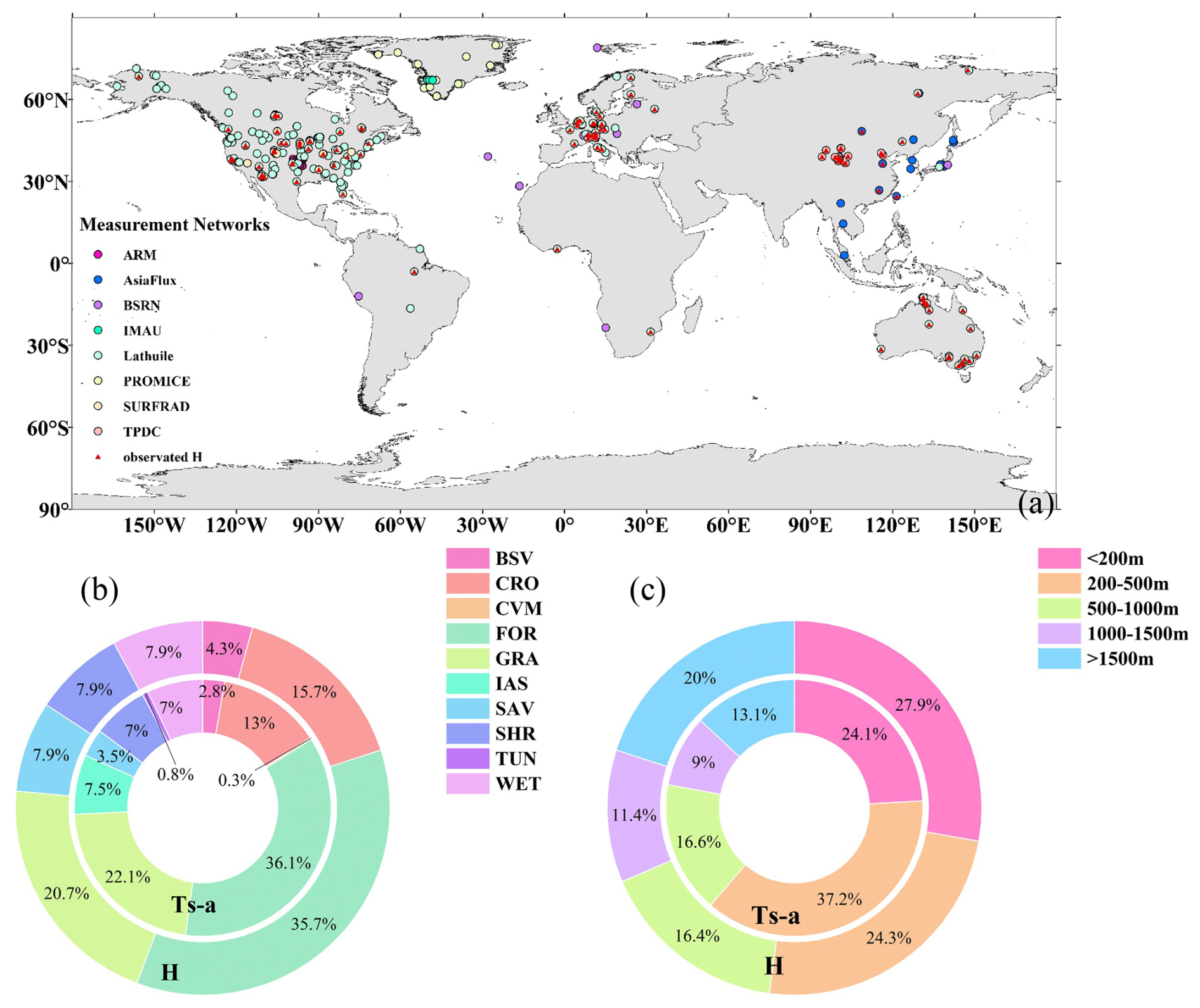
Figure 1 (a) Spatial distribution of 398 sites from eight measurement networks. The proportions of all sites for (b) ten land cover types; and (c) five elevation ranges.

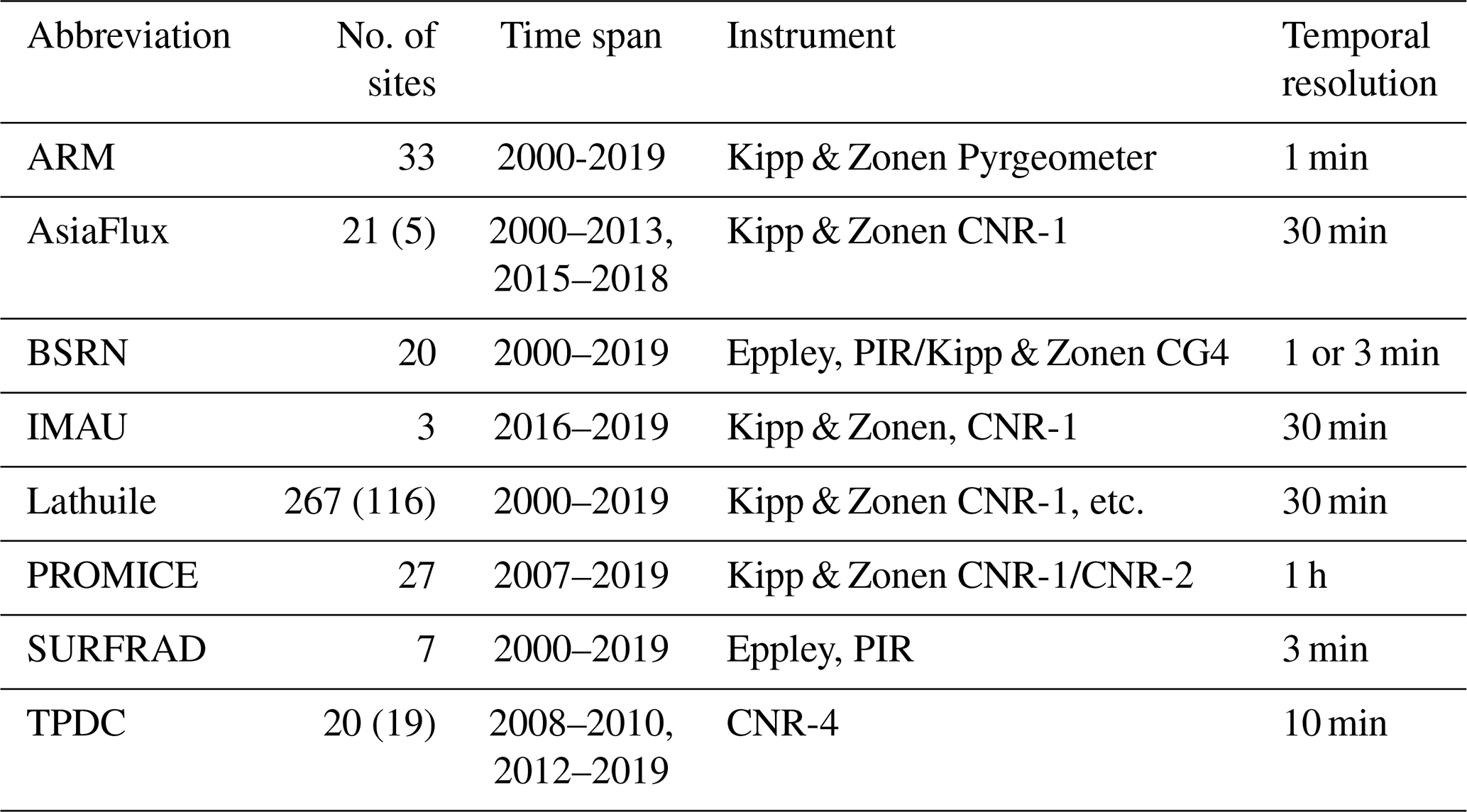
Table 2 provides detailed descriptions of the eight observation networks encompassing the 398 sites, including Atmospheric Radiation Measurement (ARM), AsiaFlux, Baseline Surface Radiation Network (BSRN), the Institute for Marine and Atmospheric Research (IMAU), Lathuile (including FLUXNET and AmeriFlux), PROMICE, SURFRAD and National Tibetan Plateau/Third Pole Environment Data Center (TPDC). Selection of sites was predicated on the availability of specific measurements: those with T_a, downward longwave radiation (DLW), and upward longwave radiation (ULW) were utilized for Ts-a calculation, whereas sites with LE, G, all four radiation components (DLW, ULW, DSR, and upward shortwave radiation 〈USR〉) or R_n were used for H estimation. As indicated in Table 2, measurement data varied in frequency and format across the sites, necessitating the conversion of all quality-controlled measurements to local time. Subsequently, different methodologies were employed to calculate daily Ts-a and H values. Ts-a was determined at an instantaneous scale using T_a, DLW, and ULW measurements according to Eq. (1). For sites recording data less frequently than hourly, Ts-a data were compiled into hourly averages, tolerating a maximum of 10 min of missing data per hour. These hourly values were then aggregated into daily means with no missing data. Conversely, daily H values were computed directly from days with over 75 % of valid observations, and subsequently adjusted for energy imbalance using the method proposed by Twine et al. (2000) (Eq. 2). R_n measurements were acquired directly from the sites or derived by summing the radiative components (Eq. 3). All calculated daily values underwent manual verification to eliminate any implausible figures. The equations below detail the procedures for calculating instantaneous Ts-a and adjusting daily H values:

$$\begin{array}{}\text{(1)}& \text{Ts-a}={\left({\displaystyle \frac{\mathrm{ULW}-(\mathrm{1}-\mathit{\epsilon })\times \mathrm{DLW}}{\mathit{\sigma }\times \mathit{\epsilon }}}\right)}^{\mathrm{1}/\mathrm{4}}-T_{\mathrm{a}}\end{array}$$

where ε represent the surface broadband emissivity and σ is the Stefan–Boltzmann constant ($\mathrm{5.67}\times {\mathrm{10}}^{-\mathrm{8}}$ W m⁻² K⁻⁴).

$$\begin{array}{}\text{(2)}& {\displaystyle }& {\displaystyle }{H}_{\mathrm{cor}}={\displaystyle \frac{R_{\mathrm{n}}-G}{H_{\mathrm{uncor}}+L{E}_{\mathrm{uncor}}}}\times H_{\mathrm{uncor}}\text{(3)}& {\displaystyle }& {\displaystyle }{R}_{\mathrm{n}}=\mathrm{DSR}-\mathrm{USR}+\mathrm{DLW}-\mathrm{ULW}\end{array}$$

where H_cor is corrected H; LE_uncor and H_uncor are uncorrected LE and H, respectively. It should be noted that this correction method relies on assumptions about the distribution of residual energy, which may still have uncertainties into the corrected flux values. These uncertainties and their potential impacts are further discussed in the Discussion section of this paper.

Table 2 The detailed information about eight observation networks.

Ultimately, a total of 649 689 daily Ts-a measurements and 216 542 daily H in-situ measurements were collected from 2000 to 2019 to estimate Ts-a and H on a global scale. Due to significant gaps in the daily in-situ measurements of H after stringent quality control, a distinct strategy was implemented to segregate the samples for H and Ts-a. For H, the methodology involved selecting monthly datasets with fewer than 10 % missing values for the training set, while the rest were allocated to an independent validation set for evaluating model performance. Linear interpolation was employed to impute missing values within the training set, ensuring the integrity of the monthly datasets. The final model was trained using 80 % of the months for training and the remaining 20 % for tuning the model parameters. This process yielded a training set encompassing 121 542 daily H samples and an independent validation set containing 97 982 samples. In contrast, the Ts-a analysis designated measurements from 2018 to 2019 as the independent validation set for model evaluation, with data from preceding years allocated to the training set. Specifically, for each site, 70 % of the samples from 2000 to 2017 were randomly selected for training, and the remaining 30 % were used for tuning the model parameters. These two approaches allow the validation set to assess the model's ability to predict “unseen” time periods and generalize to “unseen” sites (n=32 for Ts-a and 17 for H). As a result, the Ts-a training set included 564 918 daily samples, and the independent validation set comprised 84 771 daily Ts-a samples.

2.2 Remotely sensed data

2.2.1 GMTED2010 DEM

The Global Multi-resolution Terrain Elevation Data 2010 elevation dataset (GMTED2010, https://www.usgs.gov/coastal-changes-and-impacts/gmted2010, last access: 8 September 2025), developed by the United States Geological Survey (USGS), provides an advanced level of detail in global topographic data (Danielson and Gesch, 2011). It replaces Global 30 arcsec Elevation (GTOPO30) as the preferred choice for global and continental-scale applications. GMTED2010 is produced by combining multiple high-quality digital elevation model (DEM) datasets from various international institutions. This dataset offers seven raster elevation products across three spatial resolutions: 30, 15, and 7.5 arcsec. In this study, the 30 arcsec resolution product, which spans from 84° N to 90° S, was employed to derive terrain attributes such as elevation, slope, and aspect. Detailed methodologies for calculating slope and aspect are documented in the study of Liang et al. (2023).

2.2.2 GLASS product suite

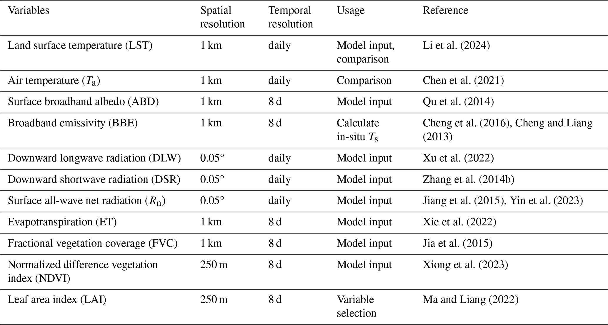
The GLASS product suite (https://www.glass.hku.hk/, last access: 8 September 2025) provides approximately 20 land surface variables with high spatial resolution (up to 250 m) and long-term temporal coverage, with many products extending from 1981 to the present. These products have gained widespread use in land surface studies, attributed to their data integrity (no missing data) and superior quality (Liang et al., 2021). The accuracy of GLASS products has been corroborated through numerous validations against in-situ measurements and other existing datasets (Yin et al., 2023; Xie et al., 2022; Yang et al., 2023). In this study, eleven GLASS products, covering the period from 2000 to 2020, were selected based on their documented impact on H variations (Zhuang et al., 2016; Trenberth et al., 2009). These products are predominantly sourced from Advanced Very High Resolution Radiometer (AVHRR) and Moderate Resolution Imaging Spectroradiometer (MODIS) observations, supplemented by other satellite and ancillary data. Comprehensive details on these eleven products are provided in Table 3. The BBE product was specifically used to acquire in-situ LST measurements, and the T_a and LST products were integrated to get GLASS Ts-a for comparison with the estimated daily Ts-a. Additionally, eight other products – surface broadband albedo (ABD), DLW, DSR, R_n, ET, FVC, NDVI and LAI – were employed to identify the optimal parameters for estimating H and to generate daily Ts-a and H estimates. Specifically, LST, DLW, DSR, NDVI were used as model inputs for Ts-a estimation, while the estimated Ts-a, in conjunction with ABD, DLW, FVC, R_n, and ET, facilitated the estimation of daily H. To maintain spatial consistency, the DSR, DLW, and R_n products, originally at a 0.05° spatial resolution, and the NDVI and LAI products, at 250 m resolution, were resampled to 1 km using the bilinear interpolation method. Subsequently, values from these products were extracted according to the in-situ measurement locations, and the 8 d composite datasets were linearly interpolated to daily values to maintain temporal alignment with the model inputs.

Table 3 Summary of eleven GLASS series products used in this study.

2.2.3 FLUXCOM

The FLUXCOM initiative (https://www.fluxcom.org/, last access: 8 September 2025) aims to improve the comprehension of the diverse sources and aspects of uncertainties in empirical upscaling, ultimately providing an ensemble of machine learning-based global flux products to the scientific community (Jung et al., 2019). It presents two product versions: one derived exclusively from MODIS satellite observations (FLUXCOM_RS) and another that integrates meteorological data from global climate forcing datasets (FLUXCOM_RS + METEO). The spatial resolution and temporal coverage of FLUXCOM_RS are constrained by its dependency on MODIS data. Moreover, both products omit unvegetated regions, including barren landscapes, permanent snow or ice, water bodies (such as Antarctica and Greenland), vast deserts (notably the Sahara), and much of the Tibetan Plateau. In this study, FLUXCOM_RS was chosen for its comparatively higher spatial resolution and marginally superior accuracy over FLUXCOM_RS + METEO. This version was utilized to assess the estimated H values derived from the LSTM model, with the annual data being interpolated to a 1 km spatial resolution for consistency.

2.3 Reanalysis data

In this study, we utilized three reanalysis datasets: ERA5, ERA5-Land, and MERRA2. The ERA5-Land was employed to evaluate the performance of the generated daily Ts-a, while all three reanalysis products were used to assess the accuracy of the generated daily H product. For the period from 2000 to 2020, all product values were initially resampled to a 1 km resolution using the bilinear interpolation method (downward fluxes considered positive). Below are detailed descriptions of these datasets:

(1) ERA5

ERA5 (https://www.ecmwf.int/en/forecasts/dataset/, last access: 8 September 2025) represents the latest iteration of the ERA reanalysis series (Hersbach et al., 2020). With its 1-hour intervals and 31 km spatial resolution, ERA5 provides enhanced spatiotemporal precision over its predecessor, the ECMWF Interim Re-Analysis (ERA-Interim). Its parameters have been widely validated and exhibit strong performance across diverse applications (Li et al., 2022a; Tarek et al., 2020; Liang et al., 2022). In this study, we converted the hourly H values from ERA5 to local time and aggregated them into daily values, which were then compared with estimated H values against in-situ measurements.

(2) ERA5-Land

The ERA5-Land (https://www.ecmwf.int/en/era5-land, last access: 8 September 2025) offers a higher spatiotemporal resolution of 1 h and 9 km. It is produced through high-resolution global numerical integrations of the ECMWF land surface model, using downscaled meteorological forcing from the ERA5 climate reanalysis. The uncertainties present in ERA5-Land are inherited from the ERA5 dataset (Muñoz-Sabater et al., 2021). In this study, we used the daily Ts-a and H values from ERA5-Land for comparison with our estimated Ts-a and H values. We converted all product values to local time and computed daily averages for comparison against in-situ measurements.

(3) MERRA2

The MERRA2 (https://gmao.gsfc.nasa.gov/reanalysis/MERRA-2/, last access: 8 September 2025) is the most recent atmospheric reanalysis from NASA Global Modeling and Assimilation Office (GMAO) at the modern satellite era. MERRA2 continues the climate record of its predecessor, MERRA, with enhancements from the updated Goddard Earth Observing System (GEOS) model and analysis program (Gelaro et al., 2017). It offers a spatial resolution of $\mathrm{1}/\mathrm{2}\mathit{°}\times \mathrm{2}/\mathrm{3}\mathit{°}$ on an hourly basis. In this study, we aggregated the hourly H data into daily values after converting them to local time.

3 Methods

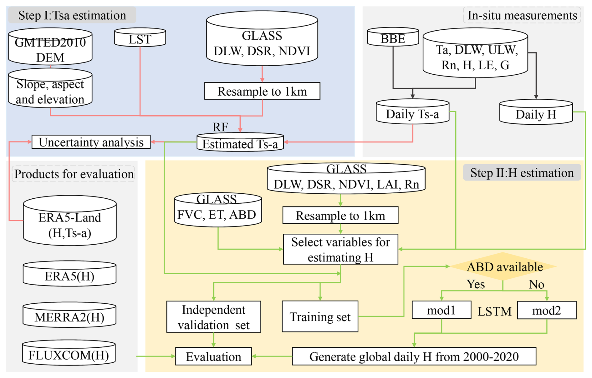
Figure 2 presents the flowchart of this study. Initially, four GLASS products (LST, DLW, DSR, and NDVI) along with GMTED2010 DEM data (including elevation, slope, and aspect) were used to estimate Ts-a through an RF model. Subsequent analysis involved in-situ Ts-a measurements and eight additional GLASS products (LAI, DSR, DLW, FVC, R_n, ABD, ET and NDVI) to identify the optimal variables for estimating H through two methods: Variance Inflation Factor (VIF) and Pearson Correlation Analysis (referred to as Pearson). Based on the analyses, five GLASS products (DLW, R_n, FVC, ET, and ABD) and the estimated Ts-a values were applied to derive H using LSTM models to account for the temporal variation of H. Considering the unavailability of ABD data during the polar night, two models were developed: mod1 for regions with ABD data and mod2 for those without, with the latter differing from mod1 only in the exclusion of ABD. The performance of all models was subsequently evaluated against in-situ measurements and other products, comparing the efficacy of H estimates across three different methods: RF, Deep Belief Network (DBN), and Transformer.

Figure 2 The flowchart of this study.

3.1 Model building of the daily Ts-a

Based on the previous studies mentioned in the Introduction section and multiple experiments, the Ts-a was estimated as:

$$\begin{array}{}\text{(4)}& T_{\mathrm{s}\text{–}\mathrm{a}}=f(\mathrm{LST},\mathrm{DLW},\mathrm{DSR},\mathrm{NDVI},\mathrm{elevation},\mathrm{slope},\mathrm{aspect},\mathrm{doy})\end{array}$$

where doy is the day of the year.

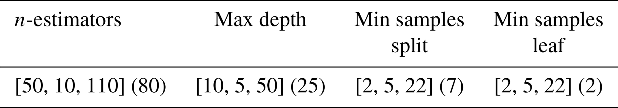
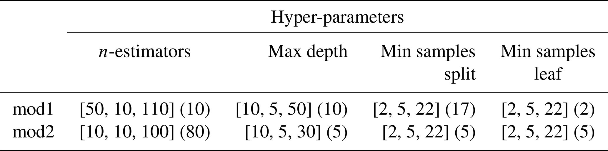
Afterwards, the Ts-a estimated model was built by using the RF method (Breiman, 1996). The RF is a widely used non-linear machine learning algorithm that constructs an ensemble of regression or classification trees. It has gained popularity in parameter prediction and estimation due to its high accuracy, ease of implementation, low computational cost, and fast processing speed (Babar et al., 2020; Liang et al., 2023; Li et al., 2022a; Jiang et al., 2023). In this study, RF regression was applied, with the final results determined by averaging the ensemble of regression output (Fig. 4a). To address common machine learning challenges such as under-fitting and over-fitting, several key hyper-parameters were fine-tuned, including the number of trees in the forest 〈n-estimators〉, the maximum depth of each tree 〈max depth〉, minimum number of samples required to split a node 〈min samples split〉, minimum number of samples per leaf 〈min samples leaf〉, and etc. (Babar et al., 2020). After plenty of experiments, we identified four hyper-parameters as critical for estimating Ts-a. To mitigate overfitting, we adopted a circular approach that minimizes the root mean-squared error (RMSE) between the training and parameter tuning in the RF model, in accordance with the methodology proposed by Li et al. (2022a). Consequently, the optimal hyper-parameters for the RF model were ascertained using these two strategies, and the results are presented in Table 4. This model is implemented on Scikit-learn toolbox (Pedregosa et al., 2012) on the Python platform within a Microsoft Windows 10 system with 32 GB of memory.

Table 4 Hyper-parameter settings used to identify optimal model for estimating Ts-a. The three values in brackets for each Hyper-parameter of every model represent the start, interval, and end values, respectively, the values in parentheses represent the value of the confirming hyper-parameter.

3.2 Model building of the daily H

3.2.1 Land surface parameters selectin

Previous studies indicate that H is influenced by a variety of land surface parameters (Nayak et al., 2022; Wulfmeyer et al., 2022). In this study, nine pertinent parameters were selected to determine the optimal variables for H estimation based on existed researches. These included three vegetation-related parameters (LAI, NDVI, and FVC) and six radiation-related parameters (Ts-a, DLW, R_n, ABD, DSR, and ET). Note that aerodynamic factors such as aerodynamic resistance, which is primarily derived from wind speed, were not included in this study. Preliminary experiments using wind speed from reanalysis datasets showed that its inclusion decreased model accuracy, likely due to the coarse spatial resolution and associated uncertainties of the data. The significant correlations among these parameters are well-established; for instance, DSR is frequently utilized to calculate R_n, while both NDVI and FVC are indices associated with LAI (Xiong et al., 2023; Jiang et al., 2015, 2023). To mitigate multicollinearity and select relevant predictors for estimating H, two statistical methods, VIF and Pearson, were employed.

VIF quantifies the degree of multicollinearity by assessing how much the variance of an estimated regression coefficient increases due to collinearity (Jiao et al., 2017; Rehman et al., 2024). As the VIF value rises, so does the degree of collinearity. A VIF value exceeding 10 typically indicates strong multicollinearity and suggests removal of the corresponding variable. The method for calculating the VIF is detailed in Eq. (5):

$$\begin{array}{}\text{(5)}& {\mathrm{VIF}}_i={\displaystyle \frac{\mathrm{1}}{\mathrm{1}-z_i^{\mathrm{2}}}}\end{array}$$

where $z_i^{\mathrm{2}}$ is the coefficient of determination when the ith independent variable is regressed against all other independent variables.

Pearson are used to measure the strength and direction of the linear relationship between two continuous variables (Pearson, 1896). This method is widely used in various fields to identify and quantify relationships between variables, understand data patterns and develop predictive models (Wei et al., 2022; Yan et al., 2023). The calculation method is presented below:

$$\begin{array}{}\text{(6)}& r={\displaystyle \frac{\sum _{i=\mathrm{1}}^n\left(M_i-\stackrel{\mathrm{‾}}{M}\right)\left(N_i-\stackrel{\mathrm{‾}}{N}\right)}{\sqrt{\sum _{i=\mathrm{1}}^n{\left(M_i-\stackrel{\mathrm{‾}}{M}\right)}^{\mathrm{2}}}\sqrt{\sum _{i=\mathrm{1}}^n{\left(N_i-\stackrel{\mathrm{‾}}{N}\right)}^{\mathrm{2}}}}}\end{array}$$

where M_i and N_i are single sample points of variables M and N, $\stackrel{\mathrm{‾}}{M}$ and $\stackrel{\mathrm{‾}}{N}$ are their means. The correlation coefficient r ranges from −1 to 1, with values closer to ±1 indicating stronger linear relationships.

Figure 3 presents the results of the multi-collinearity analysis conducted on nine land surface parameters using the two aforementioned methods. Note that the Ts-a values were obtained from in-situ measurements which considered as “true values”, while the other eight parameters were derived from the GLASS product suite. As depicted in Fig. 3a (orange bars), the VIF values for DSR, FVC, R_n, and NDVI surpass the threshold of 10, indicating the presence of multicollinearity. Given the functional relationships among FVC, NDVI, and LAI, coupled with the Pearson correlation outcomes shown in Fig. 3b, FVC was chosen due to its notably negative correlation (−0.12) in comparison to LAI (0.02) and NDVI (−0.05). Despite DSR exhibiting a higher Pearson coefficient than R_n, R_n was preferred for its applicability in nocturnal conditions and its enhanced predictive capability, potentially owing to R_n's reduced uncertainty relative to DSR, as evidenced in our experimental findings. Ultimately, six land surface parameters were selected, with none exhibiting multicollinearity issues, as illustrated in Fig. 3a (green bars).

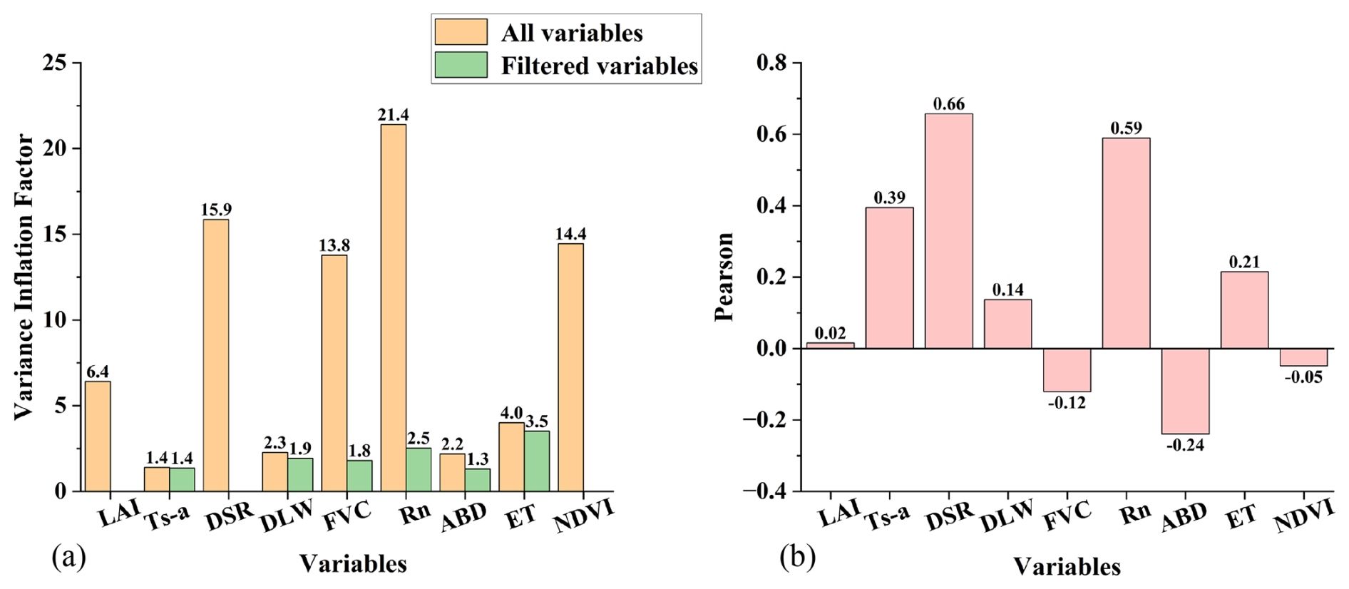
Figure 3 The results of the multi-collinearity analysis for nine land surface parameters using (a) the VIF method and (b) the Pearson method. The orange bars represent pre-filter variables, while the green bars represent post-filter variables.

3.2.2 Modeling building

According to the results presented in Sect. 3.2.1, six variables were used in estimating daily H. Furthermore, due to the unavailability of ABD data during the polar night, two models were developed: one for areas with ABD data (designated as mod1) and another for areas without ABD data (designated as mod2). Thus, the H estimation model is expressed mathematically as follows:

$$\begin{array}{}\text{(7)}& \begin{array}{rl}& H=\\ & \left\{\begin{array}{ll}f\left(T_{\mathrm{s}\text{–}\mathrm{a}},\mathrm{ABD},\mathrm{DLW},\mathrm{FVC},R_{\mathrm{n}},\mathrm{ET}\right),& \mathrm{areas}\mathrm{with}\mathrm{ABD}\\ f\left(T_{\mathrm{s}\text{–}\mathrm{a}},\mathrm{DLW},\mathrm{FVC},R_{\mathrm{n}},\mathrm{ET}\right),& \mathrm{areas}\mathrm{without}\mathrm{ABD}\end{array}\right..\end{array}\end{array}$$

Subsequently, the LSTM was used to constructed the daily H estimation model. As an advanced type of Recurrent Neural Network (RNN), LSTM effectively captures long-term dependencies by incorporating memory cells and gating mechanisms, which mitigate the vanishing gradient problem (Lyu et al., 2016; Xiong et al., 2023; Ma and Liang, 2022). In this study, both LSTM models shared the same architecture, consisting of one input layer, two LSTM layers with 400 and 250 neurons, and one regression layer (Fig. 4b). After extensive experimentation, the Adam optimizer was selected with a batch size of 16, a learning rate of 0.001, and a maximum of 100 epochs. The entire process was implemented in Python platform using the LSTM module from the Keras toolbox (https://github.com/keras-team/keras/, last access: 18 October 2025), on a Microsoft Windows 10 system with 32 GB of memory.

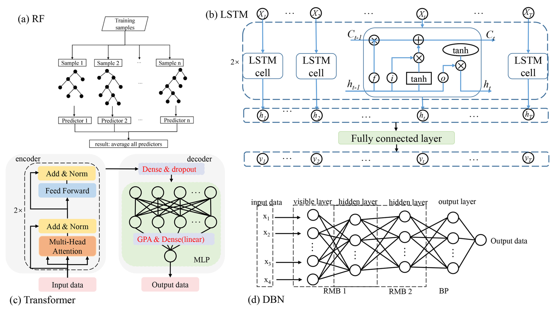
Figure 4 The structure diagram of (a) RF model, (b) LSTM, (c) Transformer model and (d) DBN model in this study. Add and Norm are the Residual Connection and Layer Normalization. GPA represents the global average-pooling operations.

3.3 Comparing daily H estimated model

Three methods were picked for their representativeness to compare with LSTM in estimating daily H, including RF, DBN and Transformer. The introduction to RF is provided in Sect. 3.1 and its optimal hyper-parameters setting is provided in Table 5. The details of the DBN and Transformer methods are described below, with their structures illustrated in Fig. 4c and d.

Table 5 Same as Table 3 but for estimating H.

(1) Deep Belief Network

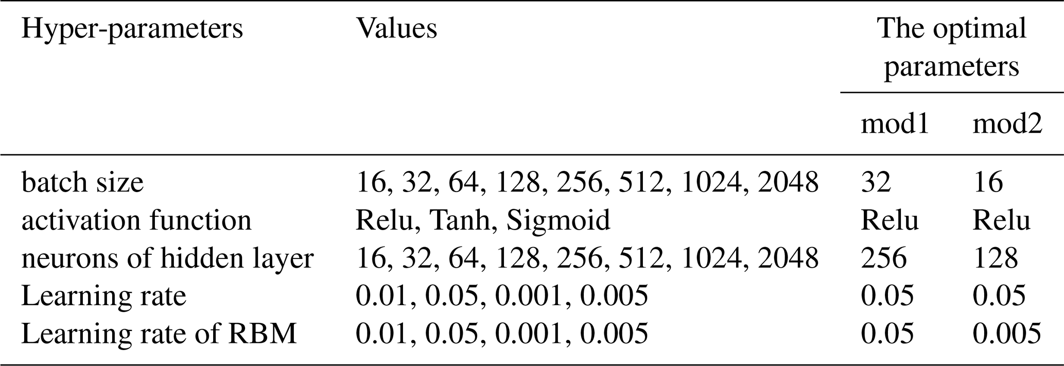
The DBN, a probabilistic generative model introduced by Hinton et al. (2006), has been widely applied in land surface parameter estimation (Zang et al., 2019; Li et al., 2017; Shen et al., 2020). It typically consists of multiple Restricted Boltzmann Machines (RBMs) and a backpropagation (BP) layer for classification or regression tasks as Fig. 4d shows. RBMs are pre-trained to capture input distributions and mitigate issues such as local optima and vanishing gradients (Hinton et al., 2006; Shen et al., 2018). In this study, the batch size, activation function, network structure, and learning rate were optimized. Following extensive experimentation, the DBN model was constructed with one RBM layer and one hidden layer, and the optimal hyper-parameter combination is provided in Table 6.

Table 6 The hyper-parameter setting for two models. The optimal parameter values for mod1 and mod2 are listed in the last two columns.

(2) Transformer

The Transformer, introduced by Ashish Vaswani et al. (2017), is a self-attention-based sequence-to-sequence model that efficiently captures long-term dependencies and enables parallel processing of input sequences, making it well suited for time series forecasting (Tay et al., 2020; Lim et al., 2021; Zhou et al., 2021). In this study, the model adopted a modified encoder-decoder architecture. The encoder included two Transformer blocks, each with a multi-head self-attention mechanism using 70 heads of size 10, followed by a feedforward network with 32 neurons. The decoder was implemented as a Multilayer Perceptron (MLP) to better suit the task. The model structure is shown in Fig. 4c.

3.4 Evaluation approaches

Three statistical measures were used to represent the validation accuracy: RMSE, Mean Absolute Error (MAE), and the coefficient of determination (R²).

$$\begin{array}{}\text{(8)}& {\displaystyle }& {\displaystyle }\mathrm{MAE}={\displaystyle \frac{\sum _{i=\mathrm{1}}^N\left|\left(Y_i-X_i\right)\right|}{N}}\text{(9)}& {\displaystyle }& {\displaystyle }\mathrm{RMSE}=\sqrt{{\displaystyle \frac{\mathrm{1}}{N}}\sum _{i=\mathrm{1}}^N{\left(X_i-Y_i\right)}^{\mathrm{2}}}\text{(10)}& {\displaystyle }& {\displaystyle }{R}^{\mathrm{2}}=\mathrm{1}-{\displaystyle \frac{\sum _{i=\mathrm{1}}^N{\left(X_i-Y_i\right)}^{\mathrm{2}}}{\sum _{i=\mathrm{1}}^N{\left(X_i-\stackrel{\mathrm{‾}}{X}\right)}^{\mathrm{2}}}}\end{array}$$

where Y_i and X_i are the estimation and the measurement values of the ith group of samples, and N represents the number of samples.

To further assess model robustness and spatial generalization, a five-fold leave-sites-out cross-validation (5-CV) was conducted for both H and Ts-a. In this procedure, all sites were split into five folds, and in each iteration, four folds were used for training while one fold was used for validation, ensuring that validation sites were excluded from the training set. The CV results complement the overall independent validation and “unseen” site evaluation, providing additional evidence of the model's ability to generalize across locations.

4 Results

4.1 Evaluation of estimated Ts-a

As described in Sect. 2.1, the measurement values from 2000 to 2017 were used for training, while data from the subsequent two years, 2018 and 2019, served as independent validation samples to assess the model's performance. Figure 5 presents the independent validation accuracy of the estimated Ts-a values using the RF model developed in this study, compared with those derived from GLASS and ERA5-Land. All three were evaluated using the same validation samples from 2018–2019 (n=83 284). For GLASS and ERA5-Land, the Ts-a values were calculated by subtracting T_a from LST.

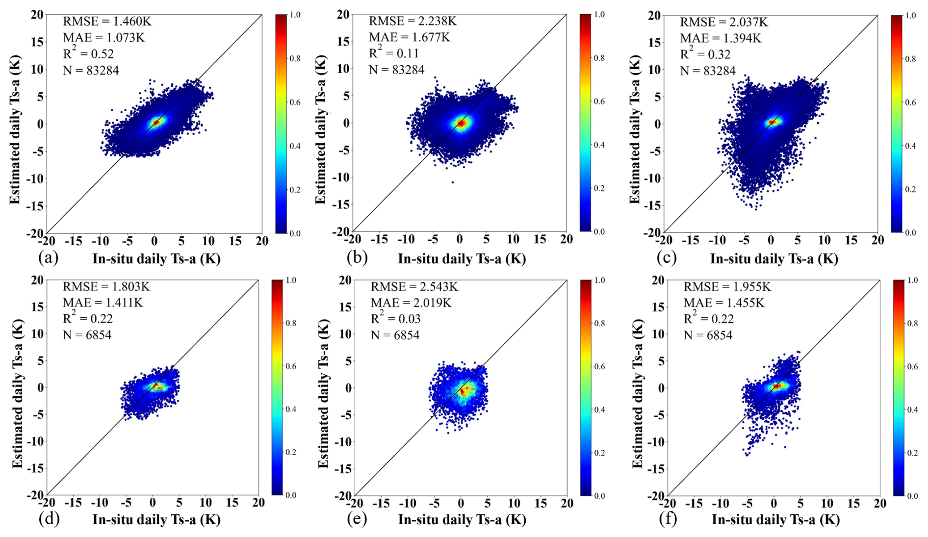
Figure 5 Comparison of the independent validation accuracy of Ts-a against in-situ measurements from 2018–2019: (a, d) estimated values using the RF model developed in this study; (b, e) from GLASS; and (c, f) from ERA5-Land. Panels (a)–(c) show results on the entire independent validation set, while panels (d)–(f) show results on the subset of “unseen” sites only.

As shown in Fig. 5a–c, the RF-estimated Ts-a over the entire validation set achieved an RMSE of 1.46 K, a MAE of 1.073 K, and an R² of 0.52, significantly outperforming GLASS and ERA5-Land, which yielded RMSEs of 2.238 and 2.037 K, MAEs of 1.667 and 1.394 K, and R² values of 0.11 and 0.32, respectively. Moreover, the estimated Ts-a values more closely align with the 1:1 line in the scatter plot, whereas GLASS shows a more dispersed distribution and ERA5-Land significantly underestimates values below 0 K. These results demonstrate that our model has strong capability for temporal extrapolation. To further examine spatial generalization, we tested the model on independent samples from “unseen” sites (Fig. 5d–f). A similar pattern is observed, with the RF model again outperforming the other two products, achieving an RMSE of 1.803 K, compared to 1.955 K for ERA5-Land and 2.543 K for GLASS. In addition, to assess model robustness, a 5-CV was conducted using all available samples. The CV results (RMSE = 1.73 K, MAE = 1.86 K, R²=0.30) are consistent with those obtained for the “unseen” sites and the temporal extrapolation tests, further confirming the strong generalization ability of the RF model. These discrepancies are likely attributable to differences in land cover types, further demonstrating the strong generalization capability of the proposed RF model in estimating Ts-a for both “future” time periods and “unseen” locations.

Building on the previously validated robustness and spatial generalization of the model, we further examined how its performance varies under different environmental conditions. Daily-scale validation accuracies of the estimated Ts-a model and two other products were evaluated using the entire independent validation set across five elevation ranges (0–200, 200–500, 500–1000, 1000–1500 and >1500 m), five NDVI ranges (0–0.2, 0.2–0.4, 0.4–0.6, 0.6–0.8 and 0.8–1), six slope ranges (0–2, 2–4, 4–6, 6–8, 8–10 and >10°) and nine land cover types (BSV, CRO, CVM, FOR, GRA, IAS, SAV, SHR and WET). These subgroup analyses focus on performance variability across different environments rather than additional “unseen” sites evaluation, providing insights into the conditions under which the model performs better or worse. The evaluation results are presented in Fig. 6.

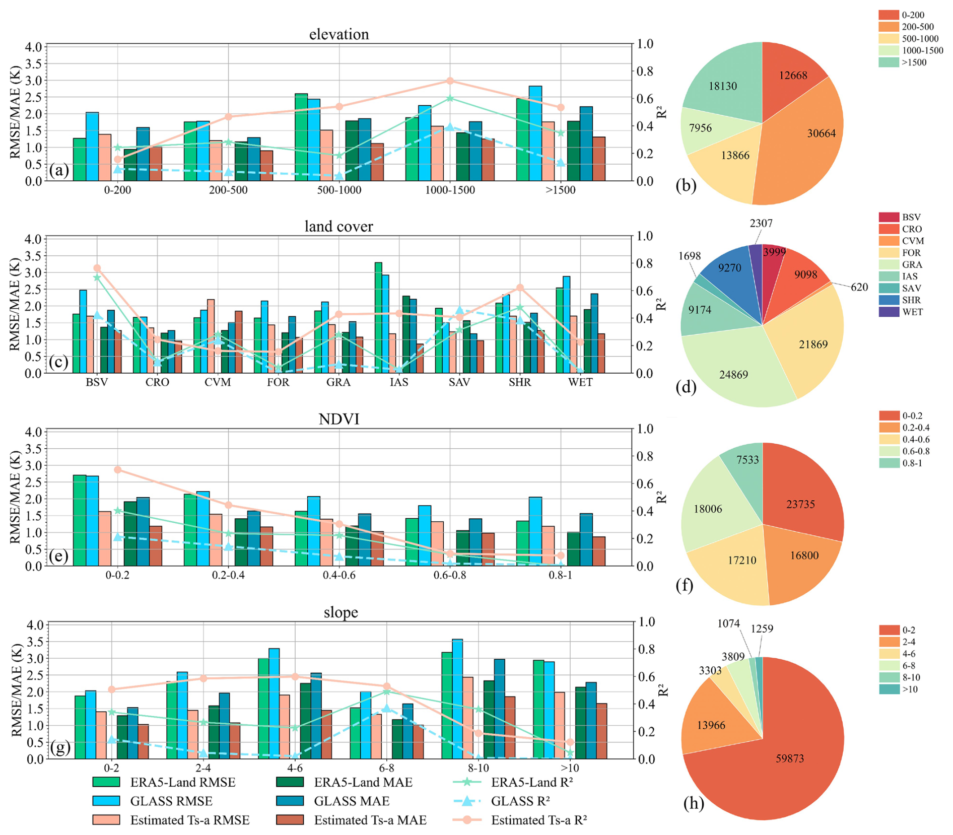
Figure 6 The validation accuracy of estimated Ts-a, ERA5-Land and GLASS across different conditions: (a) elevation within 0–200, 200–500, 500–1000, 1000–1500 and >1500 m, (b) land cover described in Fig. 1, (c) NDVI with an interval of 0.2 and (d) slope with an interval of 2°. The pie charts in (b), (d), (f) and (h) display the corresponding sample sizes for each condition.

Overall, the RF estimated model exhibited superior accuracy in various conditions, followed by ERA5-Land, aligning with findings from Fig. 5. In terms of terrain factors like elevation and slope (Fig. 6a and g), the RF model showed significant improvements, especially within the 500–1000 and >1500 m elevation ranges, and the 2–6 and >8° slope ranges, with RMSE improvements of approximately 1 K for elevation and between 0.7 and 1.4 K for slope. Regarding NDVI (Fig. 6e), a notable improvement was observed in the 0–0.2 range, with an RMSE of ∼1 K. These outcomes suggest that the RF model more accurately reflects Ts-a variations influenced by vegetation and terrain, which are key factors mentioned in the Introduction. Additionally, the performance across different land cover types was evaluated in Fig. 6c. The RF model performed well across all types, except for a site in CVM, which had an RMSE of approximately 2.2 K, an MAE of 1.8 K and R² of 0.16, slightly higher than GLASS and ERA5-Land by 0.3 and 0.5 K in RMSE, respectively. Among the eight land cover types evaluated, the RF model demonstrated exceptional performance, especially in areas with high albedo (IAS) and those subject to seasonal variations (WET). In these cases, ERA5-Land recorded an RMSE of approximately 3.3 K for IAS, while GLASS reported around 2.9 K, implying the need for caution when applying these products to studies of icy regions. Regarding the BSV, the accuracy of the RF model was on par with ERA5-Land and surpassed that of GLASS, suggesting that the RF model and ERA5-Land effectively incorporate critical information.

In summary, the accuracy of the RF model and the two comparison products varied significantly under different conditions, with the RF model consistently outperforming the others as indicated by the lowest RMSE and MAE in almost all cases. Consequently, the RF model was used to generate daily Ts-a values globally from 2000 to 2020 for the calculation of daily H.

4.2 Evaluation of model accuracy for H estimation

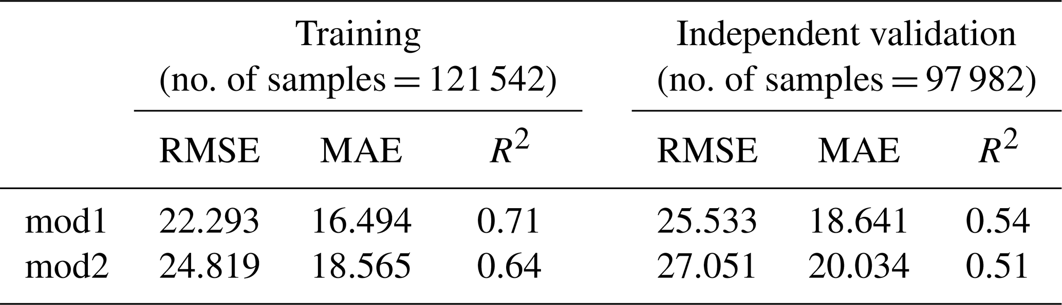
Table 7 presents the training and validation accuracy of estimated daily H from two LSTM models against in-situ measurements using the same samples. The independent validation results of two models were different but acceptable, with RMSEs of 25.533 and 27.051 W m⁻², MAEs of 18.641 and 20.034 W m⁻², and R² of 0.54 and 0.51. Compared to the training accuracy, the validation results showed a slight increase in RMSE (3.24 and 2.232 W m⁻²) and MAE (2.147 and 1.469 W m⁻²), but these differences were considered acceptable. Additionally, incorporating ABD into the model improved accuracy, reducing RMSE to 1.518 W m⁻² and MAE to 1.393 W m⁻², underscoring the significance of ABD. Overall, all models exhibited satisfactory performance, as evidenced by their comparable training and validation results.

Table 7 The training and independent validation accuracy of two LSTM models based on the same samples, both with and without the use of ABD data. Units of RMSE and Bias are W m⁻².

Due to the lack of ABD data during the polar night, two models were developed. In the final validation phase, the polar night results from model 1 were substituted with those from model 2, as depicted in Fig. 7a. The overall validation accuracy was deemed satisfactory, with an RMSE of 25.54 W m⁻², MAE of 18.649 W m⁻² and R² of 0.54. To evaluate the model's spatial generalization ability, independent validation samples were split into those from training sites and those from “unseen” sites. The corresponding accuracies are presented in Fig. 7b, where the pink scatter points represent samples from sites not included in the training process. The model performed reasonably well on the “unseen” sites, with an RMSE of 27.53 W m⁻², a MAE of 20 W m⁻² and an R² of 0.43. These results are only slightly lower than those obtained for the sites included in the training set, which yielded an RMSE of 25.16 W m⁻², MAE of 18.43 W m⁻² and R² of 0.56. In addition, a 5-CV was conducted across all samples to further assess model robustness. The CV results (RMSE = 27.9 W m⁻², MAE = 20.44 W m⁻², R²=0.49) are comparable to those obtained for the “unseen” sites, indicating that the model maintains stable performance across different data subsets. To provide a comprehensive view of site-level performance, the RMSE was calculated for each validation site, including both training sites (at previously “unseen” times) and “unseen” sites. The spatial distribution of these RMSE values is illustrated in Fig. 8. It was observed that the LSTM model exhibited the highest level of robustness on a global scale, with 80 % of the sites (107 sites) reporting an RMSE below 30 W m⁻² (indicated in red and orange in Fig. 8). Nonetheless, some sites (eight sites) displayed suboptimal performance with RMSE values exceeding 40 W m⁻².

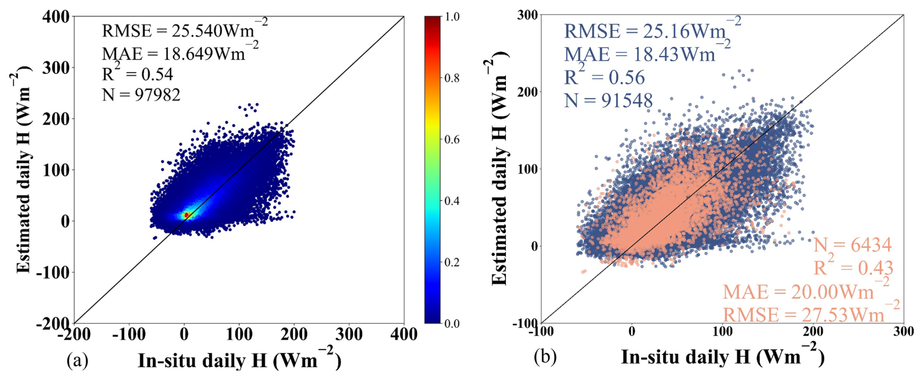
Figure 7 The accuracy of the estimated H based on (a) all independent in-situ validation samples, (b) samples from sites used in training (blue scatter points) and from “unseen” sites (pink scatter points). The values were obtained by replacing the results for areas with missing ABD in mod1 with those from mod2.

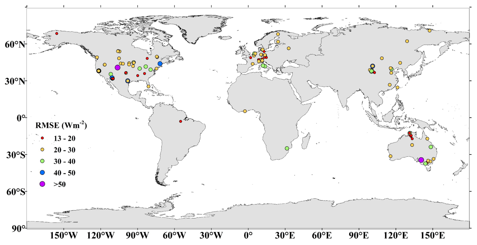
Figure 8 The spatial distribution of the validation accuracy of all sites (represented by RMSE).

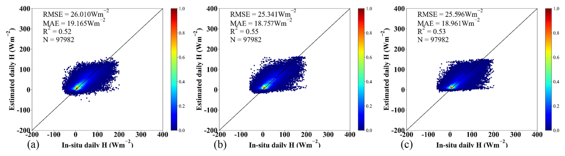
Figure 9 Validation accuracy against in-situ measurements using the common validation samples as LSTM for (a) DBN, (b) RF and (c) Transformer methods.

Afterwards, three different methods were employed to estimate H for a comparative analysis with the accuracy of the LSTM models. The independent validation results, based on the full set of samples shown in Fig. 7a are presented in Fig. 9. All comparisons were conducted using this full independent validation set to provide a comprehensive evaluation of the LSTM model against other methods, as the robustness and spatial generalization of the model have already been demonstrated in the previous analyses. The three methods produced closely aligned results, with RMSE values ranging from 25.341 to 26.01 W m⁻², MAE values between 18.757 and 19.165 W m⁻², and R² values from 0.52 to 0.55, compared to the LSTM model's RMSE of 25.54 W m⁻², MAE of 18.649 W m⁻² and R² of 0.54 (as shown in Fig. 7). However, all models exhibited varying degrees of underestimation for high values and overestimation for low values. While this issue was particularly pronounced in the Transformer and RF methods, the DBN and LSTM models demonstrated relatively better performance, albeit with similar tendencies. Remarkably, the LSTM model surpassed the DBN model, achieving improvements of 0.47 W m⁻² in RMSE and 0.516 W m⁻² in MAE. To further clarify the performance of these models, we examined each site and randomly selected three sites to illustrate the temporal variations in the values of H based on these four methods and in-situ measurements, compared against validation samples. As shown in Fig. 10, the LSTM model effectively captures the temporal variation of H in relation to in-situ measurements, while the other three models exhibit relatively poorer performance on certain days. A notable mismatch is observed in the RF, DBN, and Transformer models around the 268th day of 2012 at Lath_AU-Dry (Fig. 10a), with RF displaying only a single value and the other two methods showing underestimation on those days. Furthermore, RF and DBN exhibit opposing trends comparing to in-situ measurements during the 152nd and 218th days of 2011 at Lath_US-SRC (Fig. 10c). The variations of the four models at Lath_US-Dia (Fig. 10b) generally coincide with in-situ measurements, but RF shows slight overestimation around the 248th day of 2011 and DBN underestimates before the 196th day of 2012. Therefore, the LSTM model demonstrated superior performance, effectively mitigating the challenges of overestimating low values and underestimating high values in this study, likely due to its incorporation of time series information.

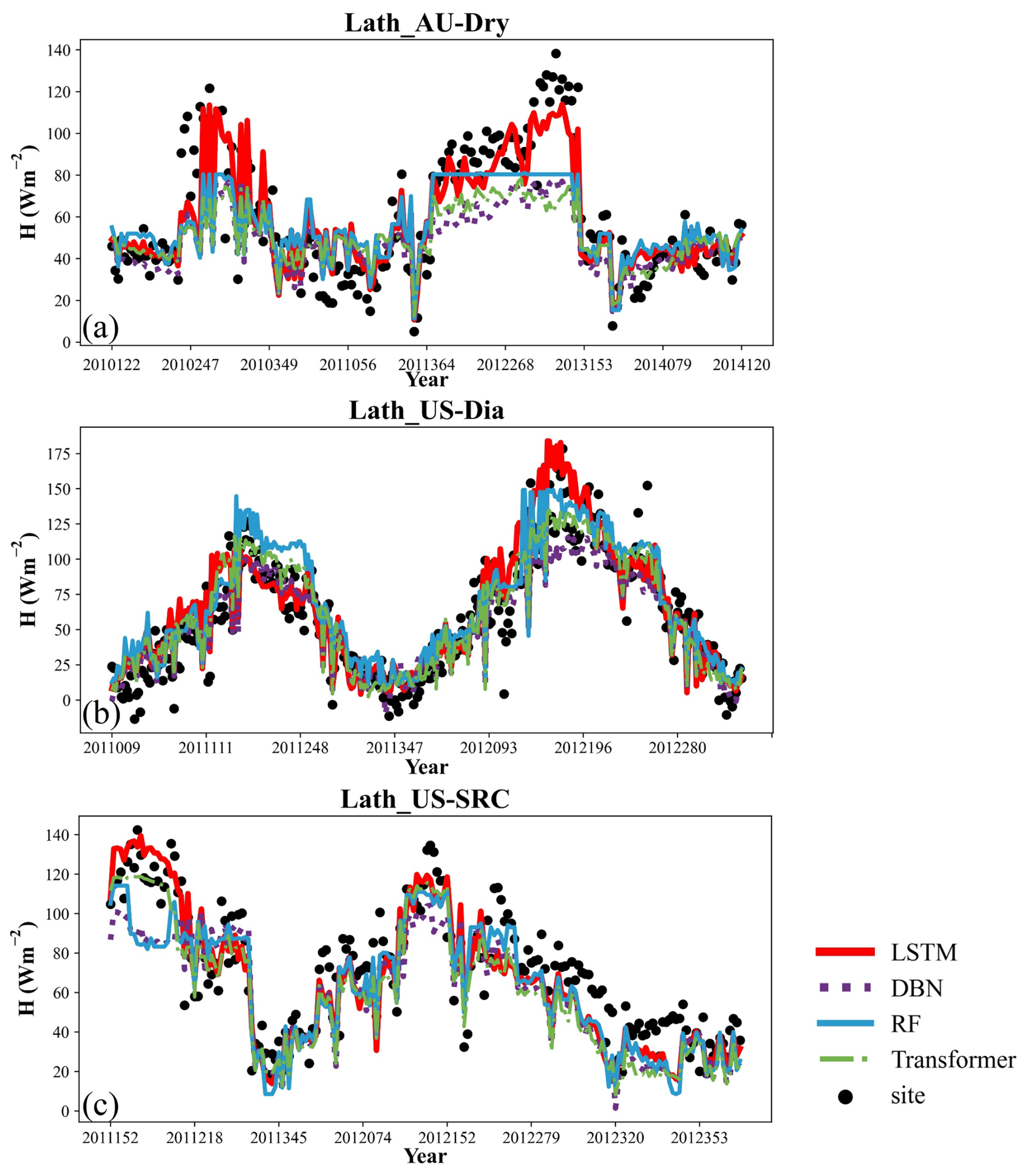
Figure 10 Temporal variations in the values of H based on the LSTM (red solid line), DBN (purple dotted line), RF (blue solid line), Transformer (green dash-dot line) and in-situ measurements (black dot) using the validation samples at (a) Lath_AU-Dry, (b) Lath_US-Dia and (c) Lath_US-SRC. Note that the time given on the abscissa is not continuous in (a)–(c).

In summary, the LSTM models employed for estimating daily H, which integrate the estimated Ts-a and other GLASS products, have shown satisfactory accuracy. Consequently, this method is deemed appropriate for global 1 km resolution mapping of daily H, establishing it as a viable and dependable approach for these applications.

4.3 Daily H product generation

In this study, daily H estimates were generated globally for the period 2000–2020 by integrating two LSTM models. Specifically, mod2 was applied under polar night conditions when ABD data were unavailable. To assess the accuracy of the estimated H, we examined its spatial and temporal variations and compared the daily estimated H values with other existing products, as outlined below.

Figure 11 Variation of monthly H in latitude zones (10°) and months zones from 2000–2020.

4.3.1 The spatial and temporal variation of H

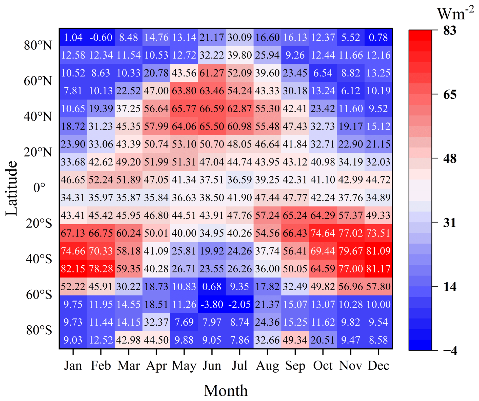
Figure 11 presents the results of calculating monthly average values across different latitude zones with a 10° range for all years. It reveals that the variation in H demonstrates distinct seasonal patterns, with higher values observed during the summer months in both hemispheres. This trend aligns with Ts-a variations, highlighting the impact of solar radiation on surface properties, which in turn affects the energy balance and flux dynamics (Jiang et al., 2022). Specifically, high H values are found in three regions: between 30–60° N from May to August, 20–50° S from January to March, and 10–50° S from October to December, peaking in January (82.15 W m⁻²) at 40–50° S. Conversely, winter months at higher latitudes exhibit low values, with the lowest recorded in June (−3.8 W m⁻²) at 60–70° S. Generally, H values in polar regions remain below 15 W m⁻², occasionally dropping below 0 W m⁻². Nevertheless, in March, April, and September, H values surpass 40 W m⁻² around 80° S. The scarcity of observation sites in polar regions might increase uncertainty in our models, particularly in the South Pole region (>70° S), thus caution is advised when using H values.

To better illustrate the spatial and temporal variations in global H during 2000–2020, Fig. 12 displays the anomaly values of land surface H across latitude zones (1°) for each day. There is a clear annual pattern influenced by the sun's position evident across these years. The position of the sun directly influences the distribution of DSR, which in turn affects Ts-a, and ultimately altering the distribution of H. Additionally, a distinct cyclic trend is noticeable in both latitudinal and temporal variations, reflecting seasonal changes across latitudinal zones and underscoring dynamic shifts in H distribution over time. These shifts may result from a combination of regional climatic changes, land surface properties, and interactions with atmospheric processes. These findings underscore the importance of long-term satellite-based remote sensing for capturing spatiotemporal variations in land-atmosphere energy exchanges. Such observations are essential for understanding the mechanisms behind energy flux dynamics and their sensitivity to environmental and climatic changes.

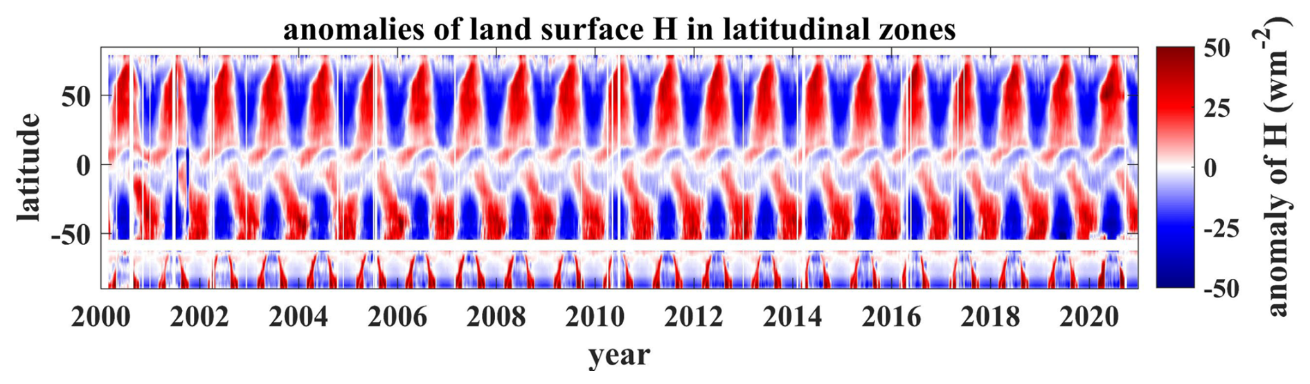
Figure 12 The anomalies of land surface H in latitude zones (1°) at daily scales from 2000–2020.

In summary, the spatial and temporal variations observed in the estimated H data align with theoretical expectations, yet they necessitate further validation. To this end, we conducted a comparison of the estimated H with other existing products to provide a more thorough evaluation.

4.3.2 Inter-comparison with other products

Three reanalysis products (MERRA2, ERA5 and ERA5-Land) and one remotely sensed-based product (FLUXCOM) were further compared. Figure 13a1–a5 illustrates the spatial distributions of these four products and the estimated H on the 121st day of 2010 at a global scale. The spatial distribution of the estimated H is logical and closely resembles that of MERRA2, ERA5-Land, and ERA5, while FLUXCOM exhibits relatively lower values compared to the other products. Additionally, we provide a further comparison of the estimated H values with other products in the Tibetan Plateau region, characterized by its complex terrain, as shown in Fig. 13b1–b5, corresponding to the black box in Fig. 13a1–a5. The spatial distribution of the three reanalysis products is noticeably smoother than that of the estimated H, and FLUXCOM lacks most data in this region. The estimated H effectively captures the intricate details of the rugged terrain, thanks to its higher spatial resolution, a detail that is not as prominently reflected in the other four products (Fig. 13c1–c5). This comparison highlights the importance of high-resolution H products for accurately depicting complex landscapes.

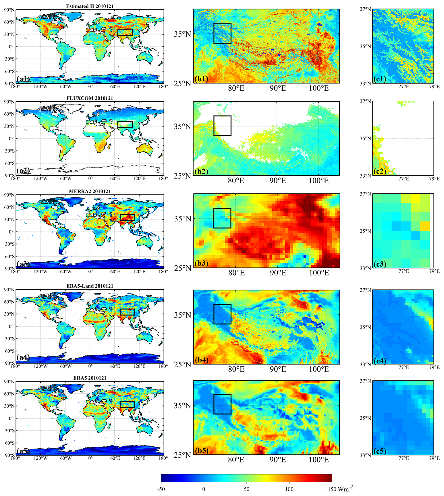
Figure 13 (a1)–(a5) display the daily values on the 121th day of 2010 for the estimated H, FLUXCOM, MERRA2, ERA5-Land and ERA5. The black box in (a1)–(a5) represents the location of (b1)–(b5) and (c1)–(c5) is the location of black box in (b1)–(b5).

Figure 13 reveals significant discrepancies in the estimated H values in certain areas compared to other products, motivating further evaluation using in-situ measurements. All subsequent results are based on the full independent validation set, as the model's robustness and spatial generalization have already been established in Sect. 4.2. To ensure spatial consistency, all products were interpolated to a resolution of 1 km. FLUXCOM_RS was evaluated separately, as it is the sole publicly available global remote sensing product that offers an 8 d temporal resolution spanning from 2001 to 2015, whereas the reanalysis products feature higher temporal resolutions (hourly) and encompass a broader timeframe (1950 to the present).

Reanalysis products

Figure 14 illustrates the performance of the estimated H values comparison to three reanalysis products (MERRA2, ERA5 and ERA5-Land), utilizing 97 045 independent validation samples. The independent validation results show that the estimated H values outperformed those of the three reanalysis products, achieving the lowest RMSE of 26.587 W m⁻² and MAE of 19.191 W m⁻². Remarkably, the estimated H exhibited significantly lower uncertainty compared to the other products, with reductions in RMSE of 9.351, 5.497 and 4.573 W m⁻² and in MAE of 6.996, 4.342 and 3.562 W m⁻² for MERRA2, ERA5-Land and ERA5, respectively. Moreover, the estimated H demonstrated enhanced accuracy for values approaching zero, in contrast to the significant uncertainty observed in the reanalysis products for small H values, potentially indicative of winter conditions (highlighted by the red circles in the Fig. 14b–d). These findings suggest that caution is advised when employing MERRA2, ERA5, and ERA5-Land for small absolute H values.

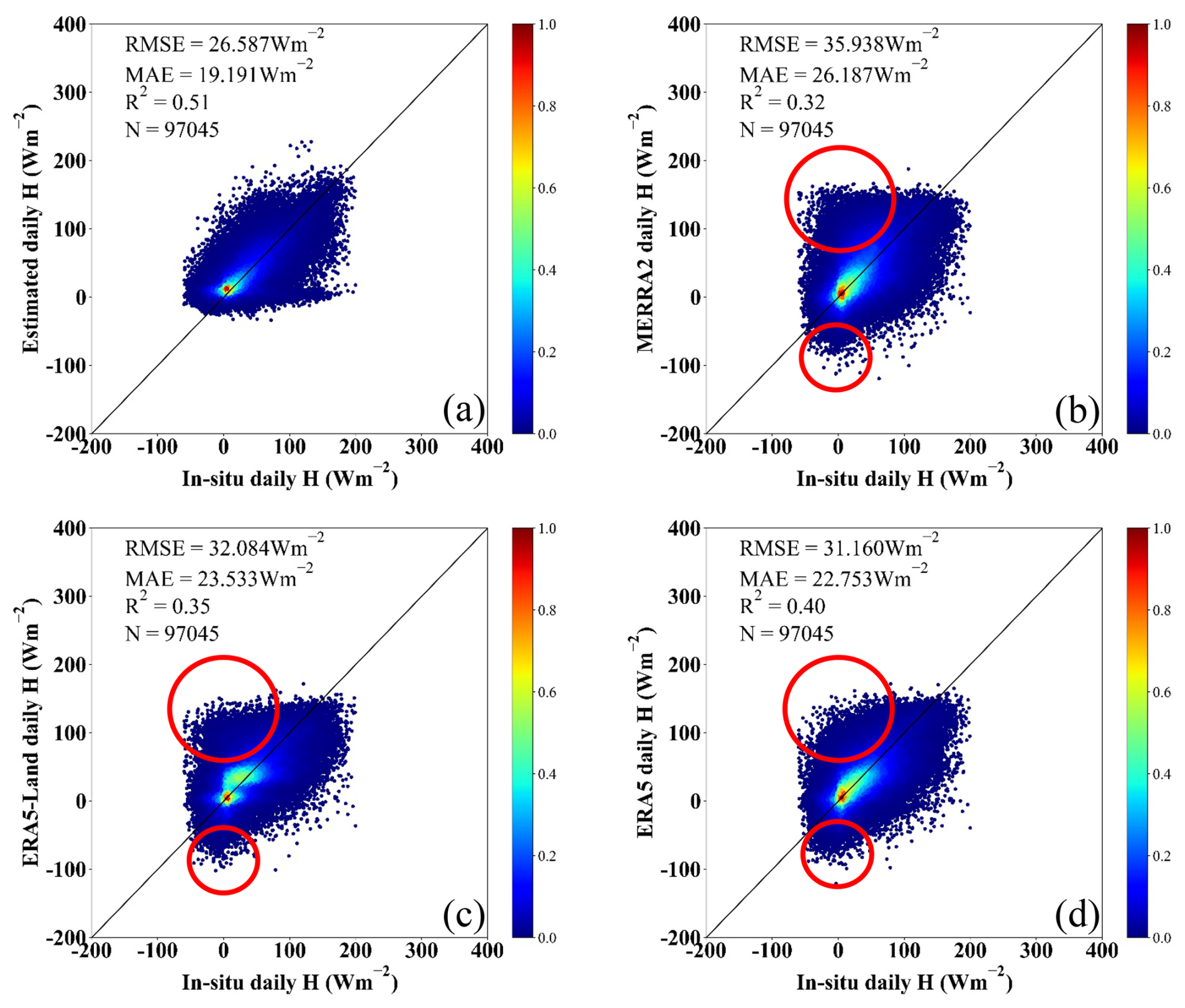
Figure 14 Comparison of the validation accuracy against in-situ measurements by using common samples in H from (a) the estimated H in this study, (b) MERRA2, (c) ERA5-Land and (d) ERA5.

Additionally, to provide a more comprehensive evaluation, we compared the performance of the estimated daily H using validation samples against three other products across seven land cover types. The comparison results, depicted in Fig. 15a–c, include RMSEs, MAEs, and R² values, while Fig. 15d provides the sample sizes for each land cover category. These results demonstrate that the accuracy of the estimated H varies by land cover type, with RMSEs ranging from 23.87 to 32.39 W m⁻², MAEs from 17.66 to 23.21 W m⁻², and R² from 0.31 to 0.58. Overall, the estimated daily H outperformed the three other datasets, followed by ERA5 (with RMSEs between 19.05 and 42.12 W m⁻² and MAEs between 14.61 and 31.58 W m⁻²), ERA5-Land (with RMSEs between 20.19 and 48.46 W m⁻² and MAEs between 15.72 and 36.34 W m⁻²) and MERRA2 (with RMSEs between 28.11 and 54.42 W m⁻² and MAEs between 21.47 and 39.46 W m⁻²). Specifically, the estimated daily H exhibited superior performance for land cover types such as WET (27.38 W m⁻² in RMSE and 19.71 W m⁻² in MAE), SHR (25.29 W m⁻² in RMSE and 18.72 W m⁻² in MAE), GRA (23.87 W m⁻² in RMSE and 17.66 W m⁻² in MAE), FOR (27.86 W m⁻² in RMSE and 19.78 W m⁻² in MAE), and CRO (26.37 W m⁻² in RMSE and 19.51 W m⁻² in MAE), with the RMSE and MAE values significantly lower than those of ERA5, ERA5-Land and MERRA. However, the estimated daily H showed marginally lower performance for SAV and BSV, with all datasets yielding relatively similar RMSEs (ranging from 25.29 to 29.7 W m⁻²) and MAEs (from 18.72 to 22.15 W m⁻²). This indicates that the estimation methods produce comparable results for these specific land cover types.

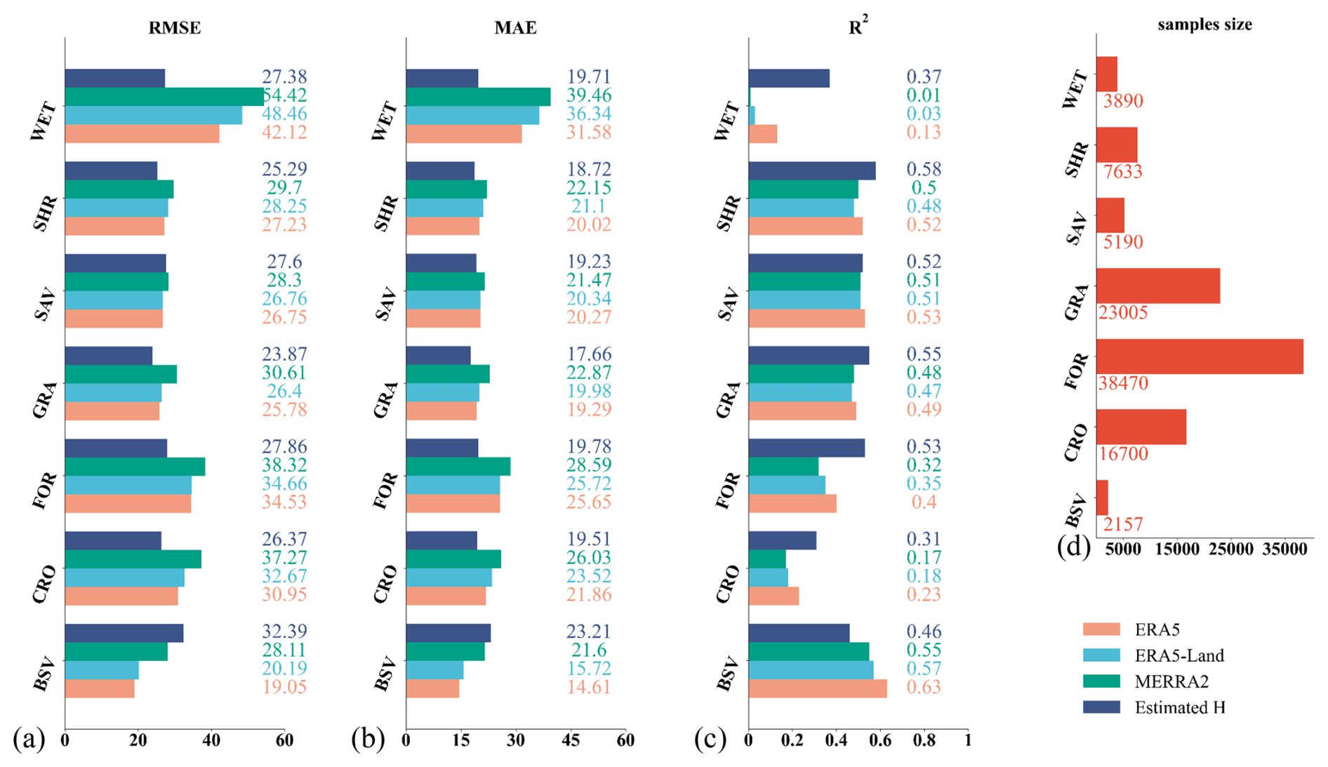
Figure 15 The (a) RMSE, (b) Bias, (c) R² of LSTM model with ERA5, ERA5-Land and MERRA2 in various land cover types. The corresponding sample size in different land cover provided in (d).

To further assess the performance across different regions, we compared the daily H estimates with other datasets using in-situ measurements across six continents, as illustrated in Fig. 16a1–a6. The comparison reveals that the estimated H achieved commendable performance in North America, Europe, Asia, and Australia, with RMSEs of 26.55, 27.15, 25.87, and 26.63 W m⁻², respectively. Notably, the RMSEs associated with the estimated H decreased significantly comparing with other three products, ranging from 5.14 to 10.21 W m⁻² in North America, 4.36 to 6.02 W m⁻² in Europe, 7.04 to 21.5 W m⁻² in Asia, and 2.42 to 8.48 W m⁻² in Australia. Conversely, the estimated H exhibited weaker performance in South America and Africa, where the validation was constrained to a limited number of sites – specifically, one site (N=548) in South America and two sites (N=1048) in Africa, as shown in Figs. 8 and 16a7. In South America, the estimated H reported an RMSE of 19.12 W m⁻², with ERA5 outperforming other datasets by achieving the lowest RMSE of 12.09 W m⁻². In Africa, the difference in RMSE between the estimated H and MERRA2 was minimal, at merely 3.03 W m⁻², whereas the greatest discrepancy was noted with ERA5-Land, which exhibited a difference of 6.53 W m⁻².

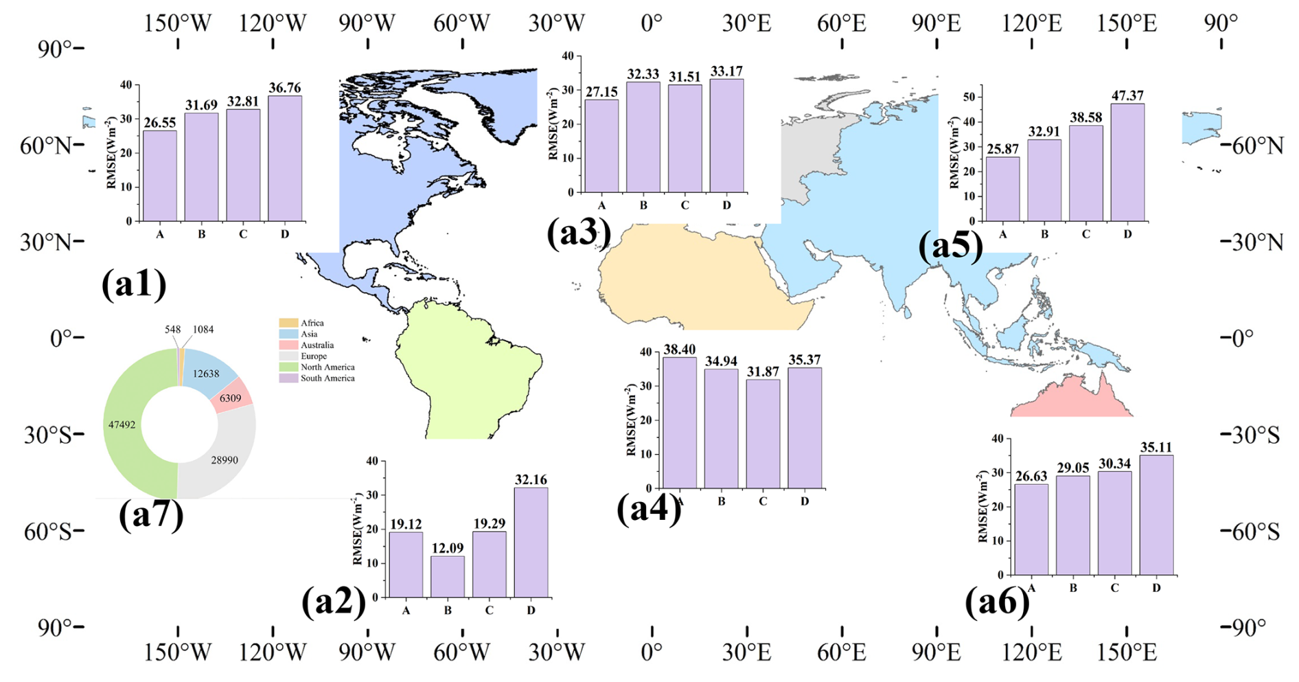
Figure 16 The RMSE values for four datasets across six continents: (a1) North America, (a2) South America, (a3) Europe, (a4) Africa, (a5) Asia, and (a6) Australia. A–D represent the estimated H, ERA5, ERA5-Land, and MERRA2, respectively. (a7) shows the corresponding sample sizes for each continent.

FLUXCOM

The H estimates derived from LSTM were compared with the sole publicly remotely sensed-based product, FLUXCOM, through independent validation samples spanning 2001 to 2015 (as shown in Fig. 17). The accuracy of the H estimates surpassed that of FLUXCOM, as evidenced by lower RMSE and MAE values of 24.5 and 18.14 W m⁻², respectively, in comparison to FLUXCOM's RMSE and MAE of 29.21 and 21.82 W m⁻² (Fig. 17a1 and b1). Furthermore, the majority of sites with estimated H exhibited RMSE values below 30 W m⁻², predominantly located in Eastern Asia, European, Eastern American, and the Northern and Southeastern regions of Australia, as depicted in Fig. 17a2 and b2. In contrast, the spatial distribution of FLUXCOM demonstrated significant variability across continents, with RMSE values ranging from 10 to approximately 40 W m⁻² even within the same continent or adjacent regions.

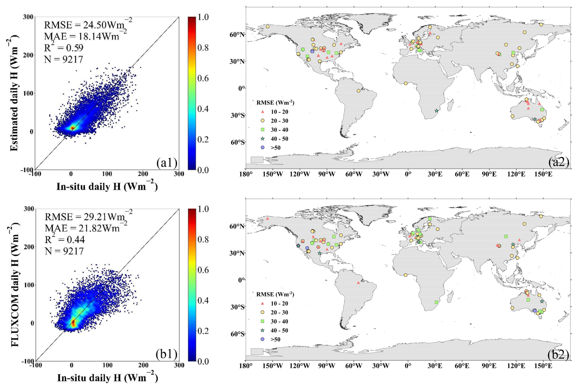
Figure 17 The overall validation accuracy against in-situ measurements by using common samples from (a1) the estimated H in this study and (b1) FLUXCOM_RS. (a2) and (b2) show their corresponding spatial distribution of site overall validation accuracy (represented by RMSE).

Based on the preceding results, the estimated H exhibits superior performance compared to FLUXCOM. To ensure a more thorough evaluation, we further assessed the validation accuracy of both products across various months, land-cover types, and elevation ranges, utilizing the same samples depicted in Fig. 18. Here, we present the RMSE values, which have been determined to accurately reflect the performance in each scenario following an extensive evaluation. Overall, the accuracy of both products exhibited variability under different conditions, yet the estimated H consistently surpassed FLUXCOM in all scenarios. Figure 18a reveals a distinct seasonal variation in accuracy, characterized by reduced RMSE values in the winter months and increased values during the summer. A similar trend was observed for R_n, which informed the derivation of H in this study (Yin et al., 2023). This seasonal fluctuation is likely due to seasonal differences in cloud cover and water vapor content, which influence radiation estimates and thus affect the H estimates. The disparity in RMSE values between the two products ranged from 1.86 to 7.5 W m⁻², with the most significant differences noted in May and June. For different land-cover types (Fig. 18b), the estimated H demonstrated stable performance, with RMSE values ranging from 24 to 30 W m⁻², indicating that the LSTM method effectively captured the features of each land cover type. In terms of accuracy for CRO and GRA, both products were comparable, with a nominal RMSE disparity of approximately 1.5 W m⁻². However, both products demonstrated relatively weaker performance in SHR, with RMSEs of 29.78 W m⁻² for the estimated H and 34.94 W m⁻² for FLUXCOM. Notably, the estimated H achieved significant improvements in WET and FOR, with RMSE improvements of 7.67 and 6 W m⁻², respectively. The comparison of accuracy across five elevation ranges is depicted in Fig. 18c. With increasing elevation, the accuracy of both products diminished. In regions exceeding 1500 m in elevation, the RMSE values reached 30.38 W m⁻² for the estimated H and 35.09 W m⁻² for FLUXCOM. Conversely, at elevations below 1500 m, the estimated H maintained a more consistent performance, with RMSE values spanning from 23.11 to 25.25 W m⁻², in contrast to the RMSE values of FLUXCOM, which varied from 26.17 to 32.05 W m⁻².

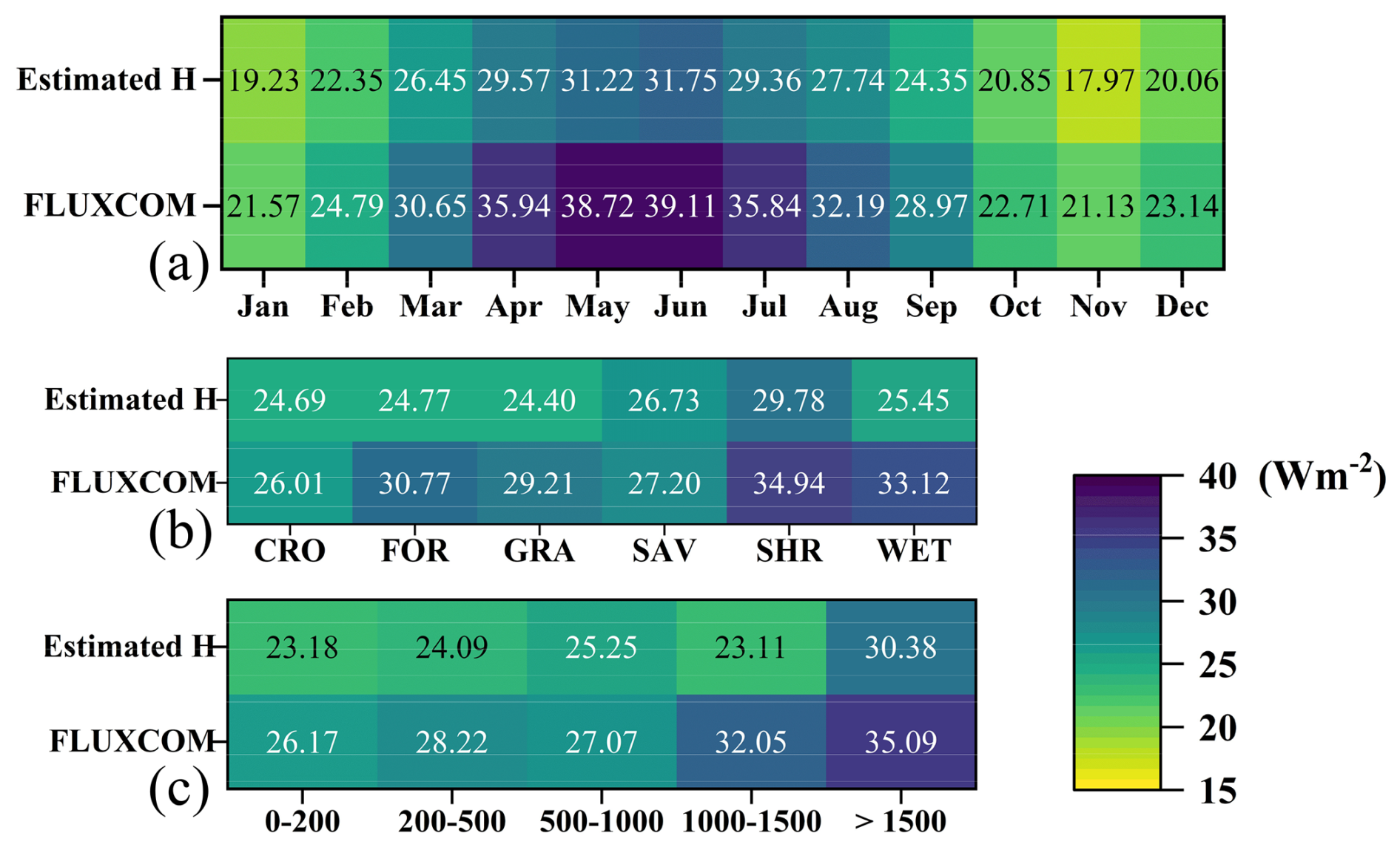
Figure 18 Comparison of the validation accuracy (represented by RMSE) in H under three conditions: (a) twelve months, (b) land-cover types and (c) elevation ranges (200, 200–500, 500–1000, 1000–1500, and >1500 m).

Overall, the daily H estimates over a 1 km resolution from 2000 to 2020, derived through the application of LSTM models based on calculated Ts-a, exhibit significant potential for broad application. This potential arises from their commendable accuracy and their proficiency in capturing surface characteristics, as compared to other existing products.

5 Discussion

Global H products encounter limitations, including coarse spatial resolution and significant uncertainties. Given that Ts-a is a crucial factor in deriving H, this study employs it to obtain H. Nevertheless, the accuracy of Ts-a calculations frequently suffers when derived from existing datasets by subtracting T_a from the LST. To overcome this limitation, we employed the RF method to estimate daily Ts-a on a global scale from 2000 to 2020, incorporating atmospheric and surface factors. Subsequently, we utilized two LSTM models to generate global daily estimates of H for the same period, based on the RF-estimated Ts-a and additional GLASS products. The performance of both RF and LSTM models is comprehensively assessed in Sect. 4, including benchmarking against various datasets and methodologies under diverse conditions. For contextual comparison, we determined the global average land surface H to be 35.29±0.71 W m⁻² over the 2000–2020 period. This value is higher than the 27 W m⁻² based on global land data from 2000 to 2004 reported by Trenberth et al. (2009), and also exceeds the 32 W m⁻² estimated by Jung et al. (2019), which excluded barren regions, deserts, permanent snow or ice, and water bodies for the period 2000–2013. It is more consistent with the 36–40 W m⁻² range reported by Siemann et al. (2018) for global land areas between 1984 and 2007. These figures are provided for general context, as differences in spatial coverage and temporal periods across studies limit direct comparability. Despite these advancements, certain aspects still require discussion, as outlined below.

5.1 Key derivers and variable importance in Ts-a estimation

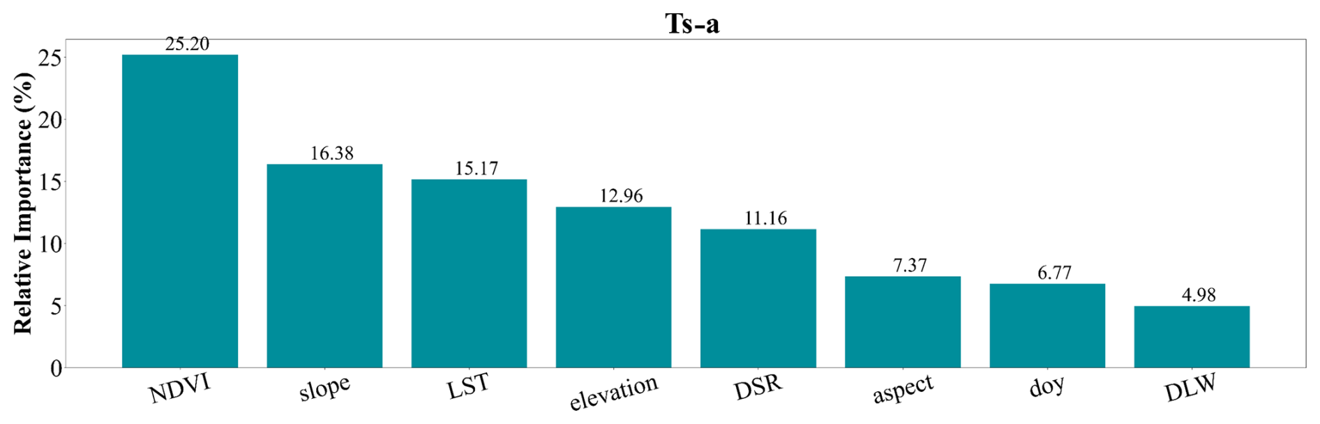
Existing research indicates that Ts-a is affected by a blend of atmospheric and surface factors (Feng and Zou, 2019). Theoretically, when the spatial resolution of terrain is finer than 5 km, it can modify the distribution of DSR and DLW reaching the land surface (Wang et al., 2004; Liang et al., 2024a), which in turn influences the distribution of LST. Variations in LST, driven by differences in terrain characteristics and land cover types, can warm the atmosphere, altering atmospheric conditions and consequently affecting radiation variation. In this study, we utilized terrain, vegetation, and radiation-related variables to estimate daily Ts-a on a global scale. The relative importance of each variable within the RF model was quantified and ranked, with the findings detailed in Fig. 19. Among the variables analyzed, the NDVI, as a key vegetation parameter, exhibited the highest relative importance score of 25.2 %. This underscores its pivotal role in estimating Ts-a. Subsequent contributors included slope, LST, elevation, and DSR, with respective importance scores of 16.38 %, 15.17 %, 12.96 %, and 11.16 %. These findings suggest that both terrain and radiation-related variables are integral to accurately estimating Ts-a. Notably, slope and elevation were more critical than the other terrain-related variable, aspect, which accounted for 7.37 %. Although flux towers are generally installed on relatively flat terrain to ensure measurement accuracy, the surrounding complex terrain within and beyond the flux footprint can still influence local surface energy and temperature dynamics near the flux towers. Similarly, LST and DSR proved to be more impactful than DLW, which held a contribution of 4.98 %. In addition, the doy ranked as the second least important variable in our analysis. Although it does not represent a direct physical environmental variable, our experiments demonstrated that it serves as a simple yet informative seasonal indicator that helps the RF model capture temporal variations effectively.

Figure 19 The relative importance (%) of each variable in RF model.

5.2 The application of accurate Ts-a

Ts-a is pivotal in influencing various land processes, boundary layer dynamics, weather forecasting, climate studies, and atmospheric profile retrievals. Its critical role extends to understanding atmospheric circulation, weather patterns, agricultural productivity, and ecological systems (Ghent et al., 2015; Zhang et al., 2014a). Previous studies have highlighted Ts-a's significant influence on summer precipitation in the middle and lower Yangtze River (Liu et al., 2009; Zhou and Huang, 2006), and its application in assessing soil desertification (Ai and Guo, 2003). Moreover, Ts-a is instrumental in reflecting various crop development stages, such as seed germination, seedling emergence, and photosynthesis, and affects soil microbial activity and the prevalence of crop diseases and pests (Gu et al., 2012). Additionally, it serves as a crucial parameter in process-based Earth system models, indicating the intensity of land–atmosphere interactions, energy fluxes, and driving key ecological and biophysical processes (Lensky et al., 2018; Qiang et al., 2011). The estimation of Ts-a in this study further facilitates the accurate derivation of T_a values. We estimated daily T_a globally by subtracting the estimated Ts-a from the GLASS LST product. For validation, we compared our T_a estimates with those from GLASS T_a using the same set of validation samples (no. of samples = 84 771). As depicted in Fig. 20, the estimation T_a achieved an RMSE of 2.621 K, a MAE of 1.971 K, and an R² of 0.95, demonstrating competitive accuracy compared to GLASS T_a (RMSE = 2.307 K, MAE = 1.692 K, R²=0.96). These results underscore the critical role of Ts-a in a wide range of environmental and agricultural applications, highlighting its significant potential for global T_a estimation and further validating the accuracy of the Ts-a model.

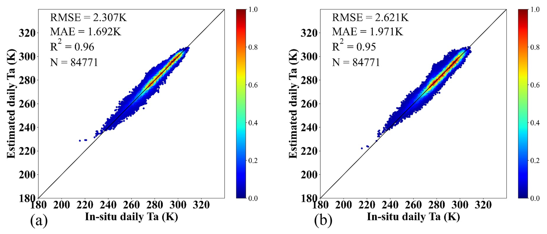
Figure 20 The direct validation result of T_a estimated by (a) GLASS T_a and (b) derived from GLASS LST and the estimated Ts-a against in-situ measurements.

5.3 Impact of Ts-a data sources on H estimation using a physical model

We investigated whether the estimated daily Ts-a could enhance the accuracy of daily H values obtained from the physical model mentioned in the Introduction, compared to other data sources typically employed in existing research. To evaluate the uncertainty introduced by varying Ts-a data sources, we calculated daily H using the temperature-derived method in Eq. (10):

$$\begin{array}{}\text{(11)}& {\displaystyle }& {\displaystyle }H=\mathit{\rho }{C}_{\mathrm{p}}\left(T_{\mathrm{0}}-T_{\mathrm{a}}\right)/r_{\mathrm{ah}}\text{(12)}& {\displaystyle }& {\displaystyle }{r}_{\mathrm{ah}}={\displaystyle \frac{\mathrm{1}}{k{u}^{*}}}\left[\ln \left({\displaystyle \frac{\left(z_{\mathrm{m}}-d\right)}{z_{\mathrm{om}}}}\right)-\mathrm{\Psi }\left(h\right)+\ln \left({\displaystyle \frac{z_{\mathrm{om}}}{z_{\mathrm{oh}}}}\right)\right]\end{array}$$

Where ρ (kg m⁻³) is the air density, C_p (J kg⁻¹ K⁻¹) is the specific heat capacity of air at constant pressure (1013), r_ah is the aerodynamic resistance to heat transfer, z_om (m) is roughness length for momentum transport, k is the von Karman's constant (0.41), u^* is friction velocity, d is zero plane displacement height, z_m (m) is the reference height, z_oh is the roughness length for heat and related to the aerodynamic parameter KB⁻¹ and z_om (KB${}^{-\mathrm{1}}=\ln (z_{\mathrm{om}}/z_{\mathrm{oh}})$), Ψ (h) represent the stability correction functions for heat, T₀–T_a represents the Ts-a and data were obtained from GLASS with 1 km resolution, estimated 1 km Ts-a using a RF model, and in-situ measurements.

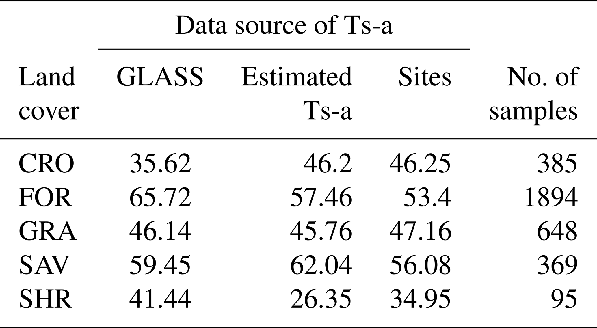
Table 8 presents the results of daily H calculated from physical model by using different data sources. A total of 3391 independent validation samples were acquired. Note that the uncertainty associated with r_ah and ρC_p were not addressed in this study. Overall, using GLASS and estimated Ts-a resulted in uncertainties of 13.5 % and 5.3 %, respectively, with RMSEs of 58.28 and 54.08 W m⁻², compared to Ts-a from in-situ measurements (RMSE = 51.35 W m⁻²). Additionally, the uncertainty varied across different land cover types, as shown in Table 8. Utilizing Ts-a from GLASS and estimated Ts-a, uncertainty ranged from 6.01 % to 23.1 %, with the highest and lowest uncertainties observed in GLASS for FOR and SAV, yielding RMSEs of 65.72 and 59.45 W m⁻², respectively. However, for certain land cover types such as CRO and GRA, lower RMSEs were noted when employing Ts-a from GLASS and estimated Ts-a compared to in-situ measurements, specifically. Specially, the RMSEs were 35.62 and 46.2 W m⁻² for CRO, and 46.14 and 45.76 W m⁻² for GRA. Moreover, across all five land cover types, RMSE values consistently exceeded 35 W m⁻² when utilizing different Ts-a data sources. This could be due to the fact that the uncertainty of parameterized method in getting r_ah was not accounted for. Therefore, accurately estimating r_ah is curial in physical model and the machine learning method used in this study effectively mitigates this issue after our experiments.

Table 8 The RMSE values of daily H calculated from physical model across five land cover types using the Ts-a obtained from GLASS, Estimated Ts-a and in-situ measurements.

5.4 Uncertainty analysis of in-situ measurements due to energy balance closure correction

As the H in-situ measurements used as ground truth values in this study have undergone energy balance closure (EBC) correction, their reliability warrants thorough discussion. In this study, we adopted the widely used method proposed by Twine et al. (2000), which redistributes the residual energy between sensible and latent heat fluxes in proportion to their original magnitudes. Although this approach has been implemented in many large-scale studies and provides a practical solution when additional constraints are lacking, recent research has underscored its limitations. Notably, Mauder et al. (2024) highlighted that EBC remains a persistent issue in FLUXNET data, with a global average energy balance ratio of approximately 0.82, and identified unresolved processes such as mesoscale secondary circulations and unmeasured energy storage terms as major contributors to the energy gap. These uncertainties are particularly relevant for H, and their effects can propagate into downstream analyses and model training. Although the Twine method does not resolve these underlying physical mechanisms, it remains a necessary and pragmatic compromise for enabling the use of flux tower data in surface energy balance studies.

6 Data availability

The daily mean values for the first three days of each year can be freely downloaded from https://doi.org/10.5281/zenodo.14986255 (Liang et al., 2025a), and the complete products are now publicly available at https://www.glass.hku.hk/ (last access: 18 October 2025).

7 Conclusions

To address the shortage of high-resolution and accurate data on daily land surface H, we employed LSTM deep learning model to produce a global daily H dataset at a resolution of 1 km for the years 2000–2020. Moreover, we introduced RF-based refined Ts-a values to enhance the accuracy of H by recognizing that Ts-a is a crucial driver of H and that significant uncertainty arises from the method of subtracting T_a from the LST. Validation against ground measurements demonstrated that this process for obtaining H is more effective than other methods and products. It successfully addressed the underestimation of high H values and the overestimation of low H values, potentially due to the incorporation of time series information. When compared to the sole satellite-based H product, FLUXCOM, this method achieved the lowest RMSE of 24.5 W m⁻² and MAE of 18.14 W m⁻², while FLUXCOM exhibited an RMSE of 29.21 W m⁻² and MAE of 21.82 W m⁻². Several conclusions can be drawn based on the results of this study: (1) H variation exhibits clear seasonal patterns akin to those of Ts-a. (2) Terrain significantly influences Ts-a estimation, with slope being the most crucial terrain-related factor. (3) The uncertainty in the physical model for estimating H was 13.5 % when using GLASS Ts-a and was reduced to 5.3 % with estimated Ts-a.

Overall, the daily H estimates derived from the LSTM method have demonstrated accuracy following extensive validation across diverse conditions and various products. However, significant uncertainties persist in the South Pole region (latitude greater than 70° S) due to data scarcity, and efforts are being made to enhance the performance in these areas. Future research should further evaluate the uncertainty of the products due to sub-pixel spatial variability and even possibly generate the high-resolution (∼30 m) H and Ts-a products using high-resolution satellite information products (Liang et al., 2024b, 2025b).