Reconstructing sea level rise from global 945 tide gauges since 1900

Tide gauges record sea level changes along coastlines. They are widely used to determine the twentieth century global mean sea level (GMSL) rise. However, a major issue in tide gauge data is the presence of various, substantial, and sometimes persistent data gaps, which hinder our understanding of sea level rise, especially at regional and local scales. Whilst the GMSL reconstructions have been provided by several influential studies, reconstructions at the exact sites of tide gauges are rarely available. Here, we present sea level reconstructions at global 945 tide gauges, covering the period from 1900 to 2022. Our approach relies on a data assimilation technique that integrates various physical sea level observations and predictions, including sea level simulations from 35 climate models. A prominent feature in our reconstruction is that it provides an ensemble of 35 reconstructions at each site of tide gauge, providing continuous and refined sea level time series. This ensemble reconstruction allows for direct statistical assessments, e.g., average, median, spread, and percentile. The average of reconstructed sea level across 945 tide gauges reveals a GMSL rate of 1.75 ± 0.05 mm yr⁻¹ over 1900–2020, and shows strong agreement with other GMSL reconstructions for both the curves of time series and overall trends. At local scale, our reconstructions are comparable to an independent reconstruction. Despite some rate differences at certain locations, the reconstructed sea level trends closely follow the raw records when they are available, emphasizing the importance of the observations at tide gauges. Our sea level reconstructions offer a valuable resource for improving global and regional sea level projections, validating climate model performance, and informing coastal adaptation strategies through understanding the sea level rise over the past century. The reconstructed sea level is available at https://doi.org/10.5281/zenodo.15385035 (Mu, 2025).

1 Introduction

Tide gauges sample relative sea level changes along coasts. The longest records date back to the early nineteenth century (Fig. 1a), according to the data collected by the Permanent Service for Mean Sea Level (PSMSL) website (https://psmsl.org/, last access: 21 December 2024; Holgate et al., 2013). Records of tide gauges are widely applied to geoscientific investigations. Extensive applications include estimating long-term sea level rise and acceleration (Douglas, 1991; Holgate, 2007; Woodworth et al., 2009); determining vertical land motion in combination with satellite altimetry (Woppelmann and Marcos, 2016; Zhou et al., 2022; Oelsmann et al., 2024); investigating the oceanic response to atmospheric loading (Ponte, 2006; Piecuch and Ponte, 2015; Zhu et al., 2024); assessing wind-driven variability along coasts (Thompson et al., 2014; Little, 2023); evaluating extreme sea level events across various time scales (Calafat et al., 2022a; Moftakhari et al., 2024); examining interaction with climate variability (Kenigson et al., 2018; Royston et al., 2022); and identifying the contributing sources to sea level rise (Frederikse et al., 2016; Wang et al., 2021; Calafat et al., 2022b; Mu et al., 2024a; Li et al., 2025). These studies highlight the essential role of tide gauges in advancing our understanding sea level changes in response to climate change.

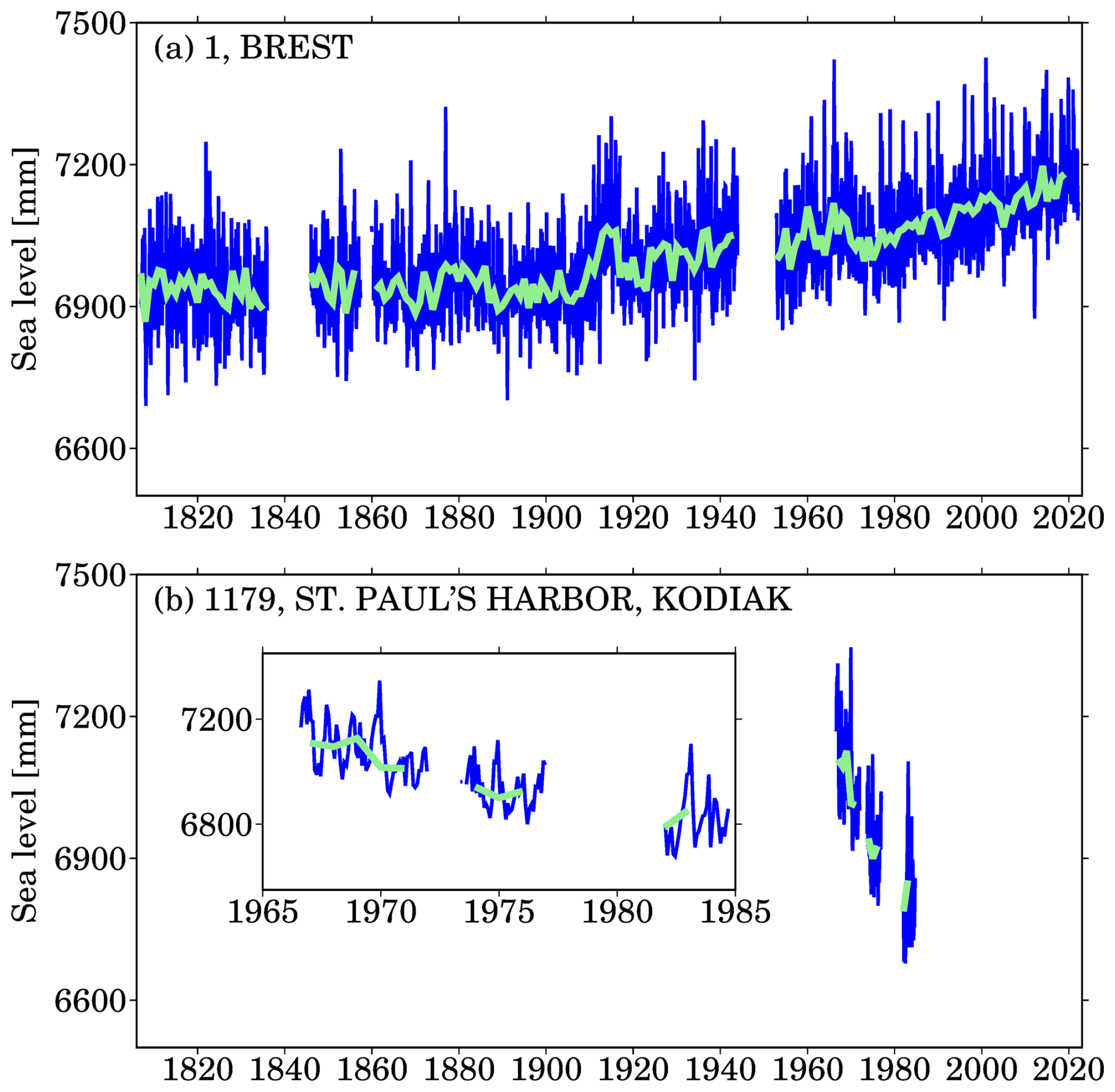
Figure 1 Examples of tide gauges from PSMSL; (a) Brest, ID 1, France; (b) St Paul's Harbor, Kodiak, ID 1179, USA; blue lines are monthly records and the light green lines are annual records.

However, a notorious issue in the records of tide gauges is the data gaps (Piecuch et al., 2017). Typical gaps are characterized by substantial discontinuity, e.g., a blank over more than decades, or only a few years, (see Fig. 1b). These data gaps may result from the site maintenance issues, instrument destruction, and complete submergence by high sea level owing to strong climate variability, such as the 1997/1998 El Niño event. Regardless of their causes, such data gaps impede applications of tide gauges in long-term sea level related studies. To address this challenge, various sea level reconstruction approaches are proposed to fill the data gaps in the tide gauge records. Classic reconstruction approaches involve empirical orthogonal function (EOF) reconstruction (Chambers et al., 2000; Church et al., 2004), and data assimilation technique (Hay et al., 2013; Calafat et al., 2022b; Mu et al., 2024b). Other strategies include station stacking (Jevrejeva et al., 2014), spatial and temporal interpolation or extrapolation using neural networks (Wenzel and Schröter, 2010) and Bayesian inference (Choblet et al., 2014; Piecuch et al., 2017).

The EOF reconstruction has been widely applied to sea level reconstruction. This approach extracts basic functions from satellite altimetry (Church et al., 2004; Church and White, 2011) or model simulations (Berge-Nguyen et al., 2008). The dominant modes (i.e., basic functions) are then combined with tide gauges to determine the amplitudes of those modes in least-square manners (Ray and Douglas, 2011). The prominent advantage of EOF reconstruction is that it produces sea level reconstruction fields with near-global coverage (matching satellite altimetry or model domains) with extension to the whole period of tide gauge records. Since the observational fields from satellite altimetry are usually removed with trends and seasonal cycles, traditional EOF reconstruction is only able to resolve the variability in sea level (Chambers et al., 2000), but not to capture the long-term trends. To address this issue, Church et al. (2004) proposed the EOF0 mode (i.e., values of ones are filled in this mode) and added it to the basic functions extracted from satellite altimetry. The resulting reconstruction retrieves the long-term trends in global sea level rise. A theoretical exploration on EOF reconstruction, especially the EOF0 component, was presented by Calafat et al. (2014). They found that, by nature, the EOF reconstruction is a weighting scheme for tide gauges. It is also should be noted that the EOF reconstruction recovers sea level changes at the predefined grids (e.g., the satellite altimetry product grids or an ocean model grid), it does not produce direct estimates at the sites of tide gauges.

A variant approach of EOF reconstruction is the cyclostationary EOF (CSEOF) reconstruction, which was developed by Hamlington et al. (2011). In contrast to the stationary basic functions from EOF, CSEOF acquires non-stationary basic functions that better describe annual cycles and some major climate variability such as the El Niño–Southern Oscillation (ENSO) (Hamlington et al., 2015). Therefore, the CSEOF reconstruction is capable of recovering non-stationary spatial variability due to ENSO, in addition to sea level rise.

Data assimilation provides another powerful framework for sea level reconstruction (Hay et al., 2013, 2015). In contrast to EOF or CSEOF methods, which are mathematically driven, data assimilation relies on physically oriented basic functions, filling the data gaps with physically meaningful interpolation/extrapolation (Mu et al., 2024a). These basic functions either describe redistributions of water mass exchange between land and oceans (Tamisiea, 2011) or represent changes in sea level due to steric effect and circulations (Gregory et al., 2019; Huang et al., 2025). The data assimilation technique was first proposed by Hay et al. (2013) in a simulation study and later applied to reconstruct the twentieth century sea level rise with 622 tide gauges. Mu et al. (2024b) modified this approach with a focus on a regional case (China coast). Their GMSL reconstruction aligns with other GMSL reconstructions. Calafat et al. (2022b) developed a different type of data assimilation to reconstruct sea level rise in the Mediterranean Sea since 1960, along with its contributing sources. Beyond reconstruction, data assimilation technique also permits for inferring ocean mass increase (Mu et al., 2024a) and sterodynamic sea level changes (Calafat et al., 2022b). The data assimilation approach can be applied to either tide gauges, emphasizing individual, local changes, or to a two-dimension field, such as satellite altimetry, resolving spatial variability (Dangendorf et al., 2024).

The spatial or temporal interpolation/extrapolation approach is implemented through several techniques. Wenzel and Schröter (2010, 2014) presented sea level reconstruction with neural networks. Their method was constructed through training neural networks with data from satellite altimetry or a reconstructed field by EOF reconstruction. A notable feature of their approach is that it is applied to monthly records rather than annual records, which thus allows the recovery of high-frequency variability. Piecuch et al. (2017) introduced a Bayesian algorithm for sea level reconstruction, and its fully Bayesian version accounts for uncertainty in model parameters. Both these studies focus on temporal interpolation/extrapolation, highlighting sea level changes at tide gauges. A distinct version of the Bayesian inference for sea level reconstruction is the trans-dimensional regression (Hawkins et al., 2019), which performs spatial interpolation/extrapolation of rates of sea level rise, rather than sea level time series. This method parameterizes Earth's surface using various structures associated with prescribed probability density functions, and generates either spatially continuous grids or specific coastal grids covering global coast (e.g., Oelsmann et al., 2024).

A conceptually straight method for sea level reconstruction is virtual station stacking (Jevrejeva et al., 2014), which merges the two closest tide gauges into a single “virtual” station and iterates this process until the virtual station converges to a final, unique station over the globe or for a given region (e.g., Pacific). Readers can see the Fig. 5 from Grinsted et al. (2007) for a direct illustration. This method creates the longest records for sea level reconstruction that dates back to 1807, and also allows for examination for regional sea level rise and acceleration (Jevrejeva et al., 2014). However, the station stacking method only permits regional or global sea level reconstruction, it does not reconstruct sea level time series at sites of tide gauges, because this method does not create interpolations or extrapolations.

To date, several notable publications (e.g., Church and White 2011; Ray and Douglas, 2011; Jevrejeva et al., 2014; Hay et al., 2015; Dangendorf et al., 2019; Frederikse et al., 2020) have already released their GMSL reconstructions to the community. These GMSL curves have been extensively applied to a range of sea level and climate studies, generating profound influence. Treu et al. (2024) released a regional sea level reconstruction whose grid covers global coast. However, this reconstruction was not performed at the exact sites of tide gauge. It involves projection from tide gauges onto satellite altimetry grids (Dangendorf et al., 2019), and spatial interpolations/extrapolations. In this study, we improve the data assimilation method (Hay et al., 2015; Mu et al., 2024a), and use it to reconstruct annual sea level changes at the exact sites of global 945 tide gauge from 1900 to 2022. Furthermore, instead of a single reconstruction time series, we offer an ensemble of reconstructions that include 35 complete time series for each tide gauges. The resulting complete records will provide valuable inputs for regional assessments of the twentieth century sea level rise, especially at regional and local scales.

2 Methods and data

2.1 Sea level reconstruction using data assimilation

In this subsection, we outline the implementation of the data assimilation approach. We begin by introducing the basic concept to facilitate understanding, followed by a detailed description of the computational procedures. The data assimilation approach consists of two fundamental stages. In the first stage, observation equations are constructed using raw records of tide gauge. In the second stage, physically oriented processes are prescribed to represent the relative sea level rise at tide gauges (Frederikse et al., 2020; Calafat et al., 2022b). These processes involve three major mechanisms. The first one is the sea level changes resulting from the ocean circulations and steric effect, which is also referred to as sterodynamic sea level (SDSL) changes (Gregory et al., 2019). We utilize outputs from the Coupled Model Intercomparison Project Phase 6 (CMIP6) climate models to represent SDSL changes at tide gauges (see Sect. 2.4). However, due to model configurations, SDSL does not account for global mean ocean mass changes (Griffies et al., 2016). To account for changes in ocean mass, we further introduce the second process that depicts the water mass exchange between oceans and land, including mass loss from the Greenland, Antarctica, and global mountain glacier, and changes in terrestrial water storage (Gregory et al., 2013). These contributions redistribute over oceans and form unique geometries under the gravity, rotation, and deformation (GRD) effect (Mitrovica et al., 2011; Coulson et al., 2022). Those oceanic geometries are termed sea level fingerprint (SLF; Coulson et al., 2022). We also introduce a random process to account for model deficiencies at local scale, because climate models tend to underestimate the sea level changes (Meyssicnac et al., 2017). The final mechanism reflects the ongoing effect from glacial isostatic adjustment (GIA) (Peltier et al., 2015), which influences the relative sea level measured by tide gauges. The three processes constitute the relative sea level rise along coast, and they have global physical origins. We therefore express the increment in sea level at tide gauges (Δ𝒮ℒ) in mathematical form:

$$\begin{array}{}\text{(1)}& \mathrm{\Delta }\mathcal{S}\mathcal{L}=\stackrel{•}{\mathcal{S}\mathcal{L}}(t{)}_{\mathrm{SLF}}\mathrm{\Delta }t+\stackrel{•}{\mathcal{S}\mathcal{L}}(t{)}_{\mathrm{SDSL}}\mathrm{\Delta }t+\stackrel{•}{\mathcal{S}\mathcal{L}}(t{)}_{\mathrm{GIA}}\mathrm{\Delta }t\end{array}$$

where ${\stackrel{•}{\mathcal{S}\mathcal{L}}}_{\mathrm{GIA}}$ is the rate of GIA relative sea level; $\stackrel{•}{\mathcal{S}\mathcal{L}}(t{)}_{\mathrm{SDSL}}$is the rate of SDSL; $\stackrel{•}{\mathcal{S}\mathcal{L}}(t{)}_{\mathrm{SLF}}$ is the rate of SLF, representing ocean mass increase.

Although the CMIP6 climate models provide SDSL estimates, they may not accurately capture local variations at tide gauge sites. To better address these local changes, we introduce a random process. Therefore, the $\stackrel{•}{\mathcal{S}\mathcal{L}}(t{)}_{\mathrm{SDSL}}$ includes two parts:

$$\begin{array}{}\text{(2)}& \stackrel{•}{\mathcal{S}\mathcal{L}}(t{)}_{\mathrm{SDSL}}=\stackrel{•}{\mathcal{S}\mathcal{L}}(t{)}_{\mathrm{Random}}+\stackrel{•}{\mathcal{S}\mathcal{L}}(t{)}_{\mathrm{Model}}\end{array}$$

Where $\stackrel{•}{\mathcal{S}\mathcal{L}}(t{)}_{\mathrm{Model}}$ is the SDSL output simulated by CMIP6 climate models, while $\stackrel{•}{\mathcal{S}\mathcal{L}}(t{)}_{\mathrm{Random}}$ is unknown variable, and will be estimated by our data assimilation framework.

Combining Eqs. (1) and (2), at a given tide gauge, its sea level at time t+1 (𝒮ℒ^t+1) can be evolved from sea level at timet(𝒮ℒ^t):

$$\begin{array}{}\text{(3)}& \begin{array}{rl}\mathcal{S}{\mathcal{L}}^{t+\mathrm{1}}& =\mathcal{S}{\mathcal{L}}^t+\stackrel{•}{\mathcal{S}\mathcal{L}}(t{)}_{\mathrm{SLF}}\mathrm{\Delta }t+\stackrel{•}{\mathcal{S}\mathcal{L}}(t{)}_{\mathrm{Random}}\mathrm{\Delta }t\\ & +\stackrel{•}{\mathcal{S}\mathcal{L}}(t{)}_{\mathrm{Model}}\mathrm{\Delta }t+\stackrel{•}{\mathcal{S}\mathcal{L}}(t{)}_{\mathrm{GIA}}\mathrm{\Delta }t\end{array}\end{array}$$

Equation (3) essentially describes how sea level rise evolves over time, or defines how sea level rise transitions from time t into time t+1. This equation contains two roles: the first one involves known variables, i.e., $\stackrel{•}{\mathcal{S}\mathcal{L}}(t{)}_{\mathrm{GIA}}$ and $\stackrel{•}{\mathcal{S}\mathcal{L}}(t{)}_{\mathrm{Model}}$, which act as the “model driven” role; the second one involves variables to be estimated through data assimilation, i.e., 𝒮ℒ(t), $\stackrel{•}{\mathcal{S}\mathcal{L}}(t{)}_{\mathrm{Random}}$, and the amplitude of $\stackrel{•}{\mathcal{S}\mathcal{L}}(t{)}_{\mathrm{SLF}}$. We stress that ${\stackrel{•}{\mathcal{S}\mathcal{L}}}_{\mathrm{SLF}}$is the overall trend of sea level fingerprint since 1900, and it is different from $\stackrel{•}{\mathcal{S}\mathcal{L}}(t{)}_{\mathrm{SLF}}$, which represents the rate of sea level fingerprint at time step t, their mathematical relation is:

$$\begin{array}{}\text{(4)}& \stackrel{•}{\mathcal{S}\mathcal{L}}(t{)}_{\mathrm{SLF}}=\mathit{\alpha }(t)\times {\stackrel{•}{\mathcal{S}\mathcal{L}}}_{\mathrm{SLF}}\end{array}$$

where αis the amplitude of ${\stackrel{•}{\mathcal{S}\mathcal{L}}}_{\mathrm{SLF}}$ at time step t. This equation implies that that their amplitudes is time variable, but the spatial pattern is fixed.

We use X^t to represent the state vector. At every time step t, the observation equation is defined as:

$$\begin{array}{}\text{(5)}& {\mathit{Z}}^t={\mathbf{H}}^t{\mathit{X}}^t+\mathit{\epsilon }\end{array}$$

where Z^t is the observational vector containing sea level records from the selected tide gauges (Sect. 2.3) at time t. Its dimension is time variable, and equals to the available number (m) of tide gauges (Fig. 2). ε denotes observational noise, and H^t is the mapping matrix, consisting of two parts:

$$\begin{array}{}\text{(6)}& {\mathbf{H}}^t=\left[\begin{array}{cc}{\mathbf{H}}_{\mathrm{TG}}^t& H_{\mathrm{other}}^t\end{array}\right]\end{array}$$

where $H_{\mathrm{other}}^t={\mathrm{0}}_{m\times (n+\mathrm{1})}$, n is the total number of tide gauges selected (for example, 945 tide gauges selected by this paper, see Sect. 2.3); ${\mathbf{H}}_{\mathrm{TG}}^t$ is sparse matrix, for each row, the ith element is one if the ith tide gauge record is available, otherwise, it is zero; the dimension of ${\mathbf{H}}_{\mathrm{TG}}^t$ is m×n.

In our data assimilation, the state vector X^t contains:

$$\begin{array}{}\text{(7)}& {\mathit{X}}^t=\left[\begin{array}{c}\mathcal{S}{\mathcal{L}}_{\mathrm{1}}^t\\ \mathrm{⋮}\\ \mathcal{S}{\mathcal{L}}_n^t\\ {\stackrel{•}{\mathcal{S}\mathcal{L}}}_{\mathrm{Random},\mathrm{1}}^t\\ \mathrm{⋮}\\ {\stackrel{•}{\mathcal{S}\mathcal{L}}}_{\mathrm{Random},n}^t\\ {\mathit{\alpha }}^t\end{array}\right]\end{array}$$

where $\mathcal{S}{\mathcal{L}}_i^t$ represents sea level at ith tide gauge at time t; ${\stackrel{•}{\mathcal{S}\mathcal{L}}}_{\mathrm{Random},i}^t$represents rate of random sea level processes at ith tide gauge; α^t is the amplitude of sea level fingerprint at time t. In the filter, the state transition matrix Φ transforms the state vector into next time step:

$$\begin{array}{}\text{(8)}& X_{\mathrm{f}}^{t+\mathrm{1}}=\mathrm{\Phi }{X}_{\mathrm{a}}^t+\stackrel{•}{\mathcal{S}\mathcal{L}}(t{)}_{\mathrm{Model}}\mathrm{\Delta }t+\stackrel{•}{\mathcal{S}\mathcal{L}}(t{)}_{\mathrm{GIA}}\mathrm{\Delta }t+w\end{array}$$

where w represents the model noise, subscript f denotes the “forecast” state, while subscript a denotes “analysis” solution. The computation of $\stackrel{•}{\mathcal{S}\mathcal{L}}(t{)}_{\mathrm{Model}}$ is detailed in the next subsection. $\stackrel{•}{\mathcal{S}\mathcal{L}}(t{)}_{\mathrm{Model}}$ and $\stackrel{•}{\mathcal{S}\mathcal{L}}(t{)}_{\mathrm{GIA}}$ serve as a driven role in our data assimilation framework and are not part of the state vector. The state transition matrix Φ is constructed as follows:

$$\begin{array}{}\text{(9)}& \mathrm{\Phi }=\left[\begin{array}{ccc}{I}_{n\times n}& I_{n\times n}& y_{\mathrm{SLF}}\\ {\mathrm{0}}_{n\times n}& I_{n\times n}& {\mathrm{0}}_{n\times \mathrm{1}}\\ {\mathrm{0}}_{\mathrm{1}\times n}& {\mathrm{0}}_{\mathrm{1}\times n}& \mathrm{1}\end{array}\right]\end{array}$$

where y_SLFcontains ${\stackrel{•}{\mathcal{S}\mathcal{L}}}_{\mathrm{SLF}}$ at tide gauges, and its dimension is n×1.

Equations (5) and (8) constitute the primary formulism of our data assimilation scheme:

$$\begin{array}{}\text{(10)}& \begin{array}{l}{\mathit{Z}}^t={\mathbf{H}}^t{\mathit{X}}^t+\mathit{\epsilon },\mathit{\epsilon }\sim N(\mathrm{0},R)\\ X_{\mathrm{f}}^{t+\mathrm{1}}=\mathrm{\Phi }{X}_{\mathrm{a}}^t+\stackrel{•}{\mathcal{S}\mathcal{L}}(t{)}_{\mathrm{Model}}\mathrm{\Delta }t\\ +\stackrel{•}{\mathcal{S}\mathcal{L}}(t{)}_{\mathrm{GIA}}\mathrm{\Delta }t+w,w\sim N(\mathrm{0},\mathit{Q})\end{array}\end{array}$$

where R denotes observation noise, and Q represents the covariance matrix of the state vector variables. The covariance structure is given by:

$$\begin{array}{}\text{(11)}& Q=\left[\begin{array}{cc}{V}_{\mathrm{TG}}& \mathrm{0}\\ \mathrm{0}& {\mathit{\sigma }}^{\mathrm{2}}{I}_{(n+\mathrm{1})\times (n+\mathrm{1})}\end{array}\right]\end{array}$$

where $I_{(n+\mathrm{1})\times (n+\mathrm{1})}$ is the identity matrix, implying that there are no correlations among random processes at tide gauges, because we assume random processes sea level and the sea level fingerprint are independent. σ² is a parameter that defines how much ${\stackrel{•}{\mathcal{S}\mathcal{L}}}_{\mathrm{Random},i}^t$ and α(t) can vary over time, in our practice, we set their value to be 1 mm yr⁻¹; V_TG defines correlation between tide gauges, and it is computed using the distance between tide gauges:

$$\begin{array}{}\text{(12)}& V_{\mathrm{TG}}={\mathit{\sigma }}_{\mathrm{TG}}^{\mathrm{2}}\left(e^{\left(-\frac{D}{\mathit{\tau }}\right)}-\mathrm{0.4}\right)\end{array}$$

where ${\mathit{\sigma }}_{\mathrm{TG}}^{\mathrm{2}}$is the variance of detrended tide gauges; τ is the decorrelation length scale, which is assumed to be 500 km; and D is the distance between tide gauges. Correlation is only considered for pairs with D≤300 km, otherwise, tide gauges are treated as uncorrelated.

The data assimilation can be solved recursively using following equations:

$$\begin{array}{}\text{(13)}& \begin{array}{l}{v}_t={\mathit{Z}}^t-{\mathbf{H}}^t{\mathit{X}}^t,F_t={\mathbf{H}}^t{P}_t{\mathbf{H}}^{t\prime }+R\\ X_{\mathrm{a}}^t={\mathit{X}}^t+P_t{\mathbf{H}}^{t\prime }{F}_t^{-\mathrm{1}}{v}^t,P_{\mathrm{aa}}^t=P_{\mathrm{f}}^t-P_{\mathrm{f}}^t{\mathbf{H}}^{t\prime }{F}_t^{-\mathrm{1}}{\mathbf{H}}^t{P}_{\mathrm{f}}^t\\ X_{\mathrm{f}}^{t+\mathrm{1}}=\mathrm{\Phi }{X}_{\mathrm{f}}^t+K_t{v}_t,P_{\mathrm{f}}^{t+\mathrm{1}}=\mathrm{\Phi }{P}_{\mathrm{f}}^t(\mathrm{\Phi }-K_t{\mathbf{H}}^t{)}^{\prime }+Q\end{array}\end{array}$$

where $K_t=\mathrm{\Phi }{P}_{\mathrm{f}}^t{\mathbf{H}}^{t\prime }{F}_t^{-\mathrm{1}}$ is the Kalman gain matrix, and v_t is the innovation with variance F_t (Didova et al., 2016).

In the smoother (i.e., the backward loop) process, the Kalman smoother comprises the equations:

$$\begin{array}{}\text{(14)}& \begin{array}{l}{r}_{t-\mathrm{1}}={\mathbf{H}}^{t\prime }{F}_t^{-\mathrm{1}}{v}_t+L_{t\prime }{r}_t,N_{t-\mathrm{1}}={\mathbf{H}}^{t\prime }{F}_t^{-\mathrm{1}}{\mathbf{H}}^t+L_{t\prime }{N}_t{L}_t\\ {\stackrel{⌢}{X}}^t={\mathit{X}}^t+P_t{r}_{t-\mathrm{1}},V_t=P_t-P_t{N}_{t-\mathrm{1}}{P}_t\end{array}\end{array}$$

where $L_t=\mathrm{\Phi }-K_t{\mathbf{H}}^t$, and ${\stackrel{⌢}{X}}^t$ represents the smoothed state vector.

2.2 Instantaneous rate of SDSL changes

The instantaneous rate of SDSL changes $\stackrel{•}{\mathcal{S}\mathcal{L}}(t{)}_{\mathrm{Model}}$ acts as drivers in our data assimilation framework. Two essential computational steps are employed to determine $\stackrel{•}{\mathcal{S}\mathcal{L}}(t{)}_{\mathrm{Model}}$. First, we extract the low-frequency variations x(t) from a given SDSL time series simulated by CMIP6 climate models. Second, we estimate the instantaneous rate by computing the first-order temporal derivative of x(t).

Given a raw time series y(t) with unit of millimetre, we apply Hodrick-Prescott (HP) filtering (Kim et al., 2009) to extract its low-frequency variation:

$$\begin{array}{}\text{(15)}& x^{\mathrm{HP}}={\left(I+\mathrm{2}\mathit{\lambda }{T}^{\prime }T\right)}^{-\mathrm{1}}y\end{array}$$

where T is Toeplitz matrix:

$$\begin{array}{}\text{(16)}& \mathbf{T}=\left[\begin{array}{ccccccc}\mathrm{1}& -\mathrm{2}& \mathrm{1}& & & & \\ & \mathrm{1}& -\mathrm{2}& \mathrm{1}& & & \\ & & \mathrm{\ddots }& \mathrm{\ddots }& \mathrm{\ddots }& & \\ & & & \mathrm{1}& -\mathrm{2}& \mathrm{1}& \\ & & & & \mathrm{1}& -\mathrm{2}& \mathrm{1}\end{array}\right]\end{array}$$

Based on the x^HP, we estimate the instantaneous rate $\stackrel{•}{\mathcal{S}\mathcal{L}}(t{)}_{\mathrm{Model}}$ by taking the first-order temporal derivative. Since climate model historical outputs cover the period 1900–2014, the instantaneous rate is only available for this period. For the extension period of 2015–2022, we assume that the instantaneous rates remain the same rate as the year of 2014, and construct a complete time series for 1900–2022.

In HP filtering, the smoothed time series are affected by the parameter lambda. To illustrate this effect, we select the SDSL time series from the ACCESS-CM2 model interpolated at tide gauge Den Helder (PSMSL ID 23) and Buenos Aires (PSMSL ID 157), then perform the HP filter with lambda = 1, 10, 100, and 1000, respectively (Fig. 2). We can observe that a large lambda produces a refined curve that suffers from less high-frequency variability or better represents the low-frequency variability. In our practice, we adopt the value of 10, as it shows smaller peak-to-peak variations. This choice is empirically determined. This smooth curve is then used to compute the instantaneous SDSL rates that drive the data assimilation.

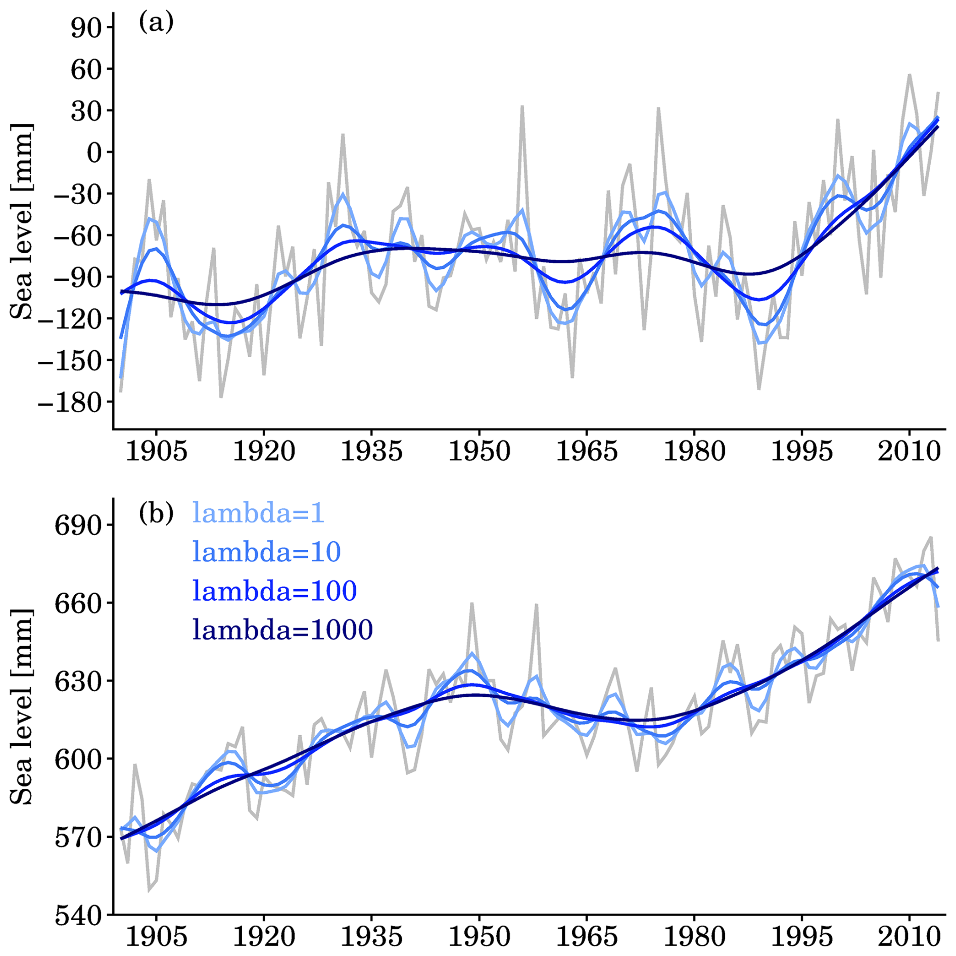
Figure 2 The effect of lambda on the smoothed time series by HP filter. Gray lines are raw SDSL time series from ACCESS-CM2 model (see Table 1) at tide gauges (a) Den Helder (PSMSL ID 23) and (b) Buenos Aires (PSMSL ID 157).

2.3 Tide gauges

We consider annual records of tide gauges collected by the PSMSL website (https://psmsl.org/, last access: 21 December 2024; Holgate et al., 2013). The PSMSL database stored more than 1500 tide gauges that are distributed along the global coastline (Fig. 3; data access on 26 November 2024). However, many tide gauge records exhibit substantial data gaps, suspicious anomalies, or abrupt jumps (e.g., Piecuch et al., 2017; Oelsmann et al., 2024). Previous studies (Church and White, 2011; Ray and Douglas, 2011; Jevrejeva et al., 2014; Hay et al., 2015; Wang et al., 2024; Mu et al., 2024a) have applied various selection criteria to identify reliable tide gauges based on specific research objectives.

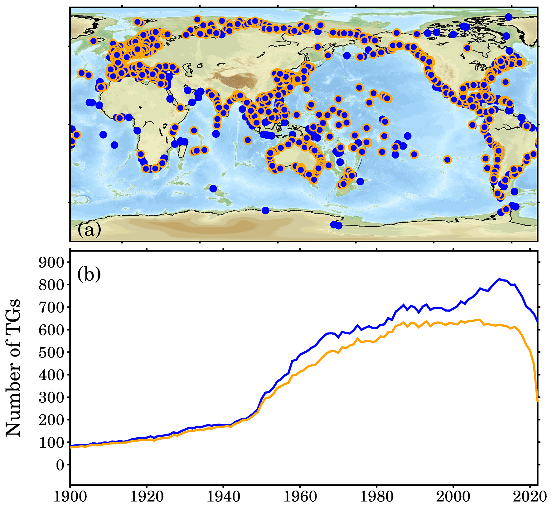
Figure 3 Tide gauges from the PSMSL (access on 25 January 2025). (a) Distribution of all tide gauges, and those marked with orange circles are selected in this study. (b) The available numbers of tide gauges: the blue line represents all available tide gauges, while the orange line includes only the selected subset. The apparent decline toward the end of the record is primarily due to delays in data updates.

In this study, we adopt a single primary criterion: tide gauges must have at least 20 years of data within the period 1900–2022. We do not exclude records with large jumps or high rates, as their impact on global sea level reconstruction is negligible. After applying this criterion, 945 tide gauges are retained. Figure 3b shows the number of available records for every year over 1900–2022. The orange line represents the records selected by this study. Notably, most pre-1950 records are included, although their number is relatively small – fewer than 300 in total and fewer than 100 during 1900–1910. Over 1900–2022, these 945 tide gauges could potentially provide 116 235 (945 × 123) data records. However, due to data gaps, only 45 682 records are available, including anomalous records, accounting for only 39.3 % completeness over all. Note that the completeness is time variable (see Fig. 3b), it is even worse before 1950.

2.4 Climate models

Table 1 35 CMIP6 models.

In our assimilation framework, we have adopted the SDSL changes estimated by the CMIP6 climate models (Griffies et al., 2016). The SDSL changes describe fluctuations that are attributable to ocean dynamics. This diagnostic field is expected to have a zero global mean (Gregory et al., 2019). Therefore, it does not capture the component of GMSL changes contributed by the ocean mass increase due to polar ice melting and terrestrial water storage variations. Totally, we include 35 CMIP6 climate models that provide both monthly gridded SDSL fields and the global mean thermosteric sea level changes (Table 1 and Fig. 4). We first remove the global mean of original gridded fields, if they are not zero, and then add the global mean thermosteric sea level time series back to the gridded fields. Most of the global mean thermosteric sea level time series from CMIP6 climate models appear to have positive trends. However, there are two of them showing negative trends, contradicting the observations (e.g., Frederikse et al., 2020). Despite this inconsistency with observations, we retain these two models, because they contribute to the diversity in CMIP6 models.

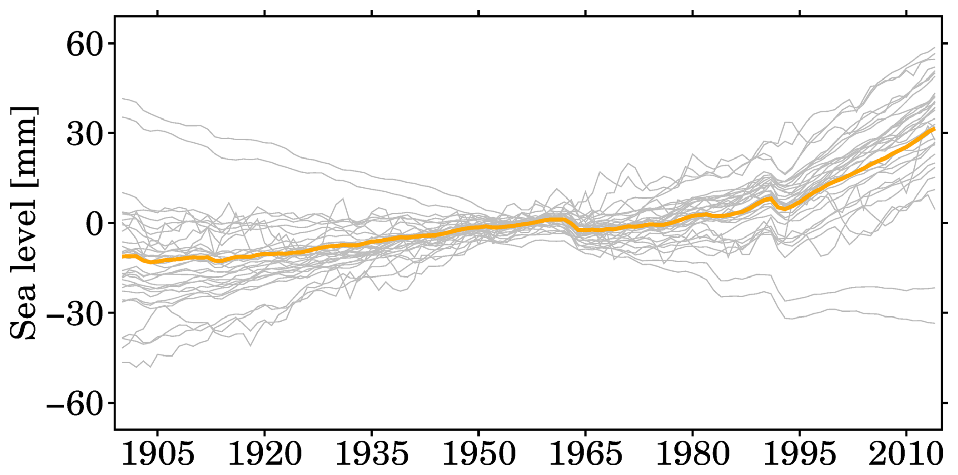
Figure 4 Global mean thermosteric sea level rise from CMIP6 climate models. Gray lines indicate individual results from 35 climate models, and orange line indicates their ensemble mean.

2.5 Sea level fingerprints

Water mass exchanges between land and oceans involve four major processes: (1) the mass loss or gain in global glaciers; (2) the mass loss from the Greenland Ice Sheet; (3) the mass loss from the Antarctica Ice Sheet; and (4) variations in terrestrial water storage, driven by both internal nature variability and external anthropogenic forcing. When additional waters from these sources enters the ocean, it inevitably contributes to global sea level rise. However, this rise is not spatially uniform. Instead, it exhibits a distinct spatial pattern due to the combined effects of GRD (Farrell and Clark, 1976; Mitrovica et al., 2011; Adhikari et al., 2016). The resulting spatial pattern is known as the SLF, which characterizes the Earth's response to surface mass loading redistribution. Given the centennial timescale considered in this study, we focus solely on the Earth's elastic response. We adopt the total SLF provided by Frederikse et al. (2020), which represent the integrated contributions from the four global land-based mass redistribution processes (Fig. 5). These individual SLF processes are gridded into 0.5° grid, covering the period from 1900 to 2018. We use this dataset to estimate the overall long-term SLF trend.

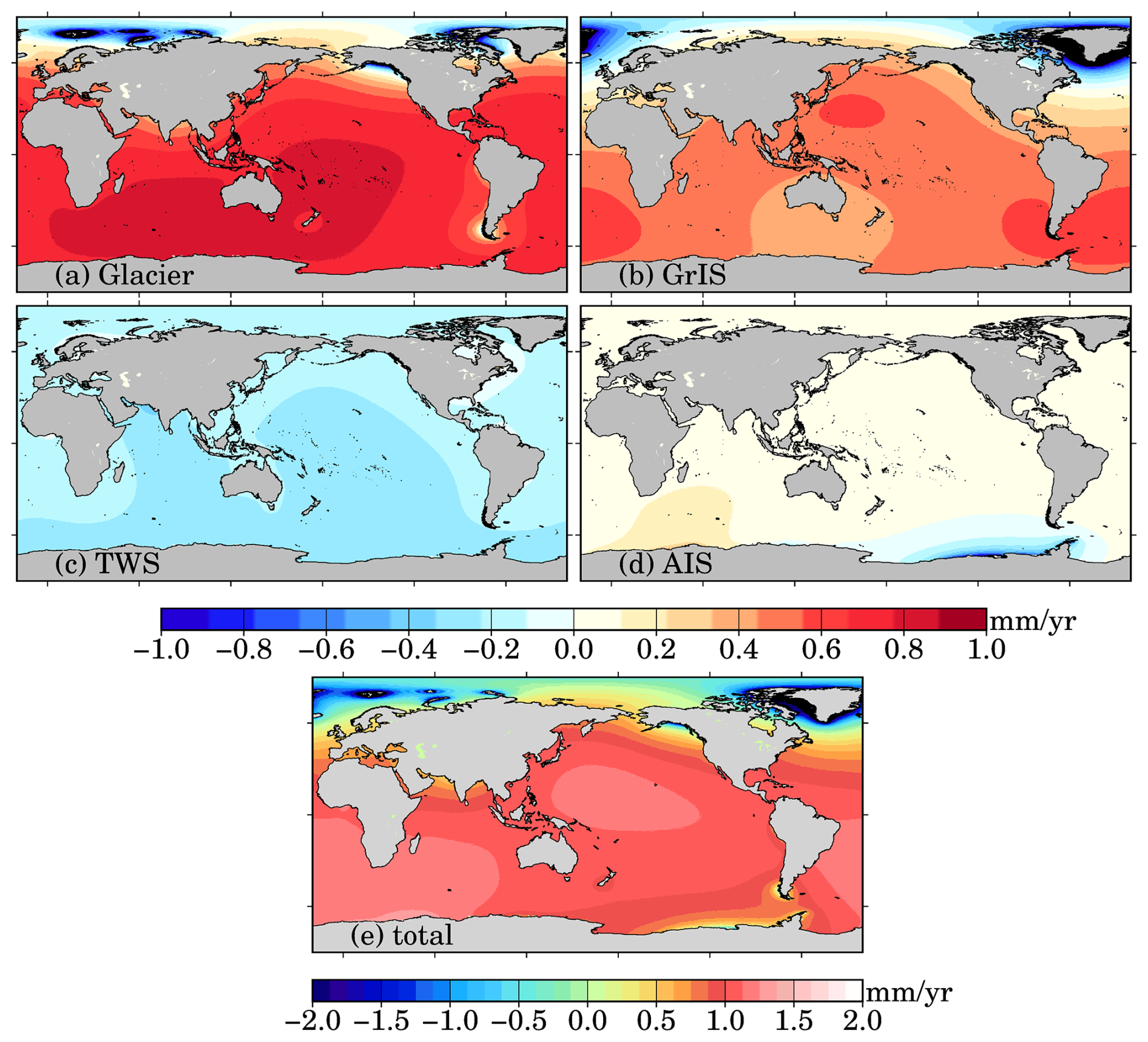
Figure 5 Sea level fingerprints caused by (a) global mountain glacier, (b) Greenland Ice Sheet, (c) terrestrial water storage variations, (d) Antarctic Ice Sheet, (e) the total sea level fingerprints.

2.6 Glacial isostatic adjustment

The data assimilation technique in this study also requires relative sea level rise contributed from GIA effect. We use model outputs from ICE-6G-C model (Peltier et al., 2015). Figure 6 shows the spatial pattern of the relative sea level rise from the ICE-6G-C model. The GIA-induced relative sea level is assumed to be purely linear changes for the period from 1900 to 2022, as the GIA-induced relative sea level is mainly an ongoing response to the tremendous ice melting since the Last Glacial Maximum (Calark et al., 2009). In addition, GIA effect also induces an uplift change, i.e., vertical land motion (Hamlington et al., 2016; Woppelmann and Marcos, 2016; Santamaría-Gómez et al., 2017). The GIA-induced relative sea level rates at all 945 tide gauges are also included in our data files (Mu, 2025).

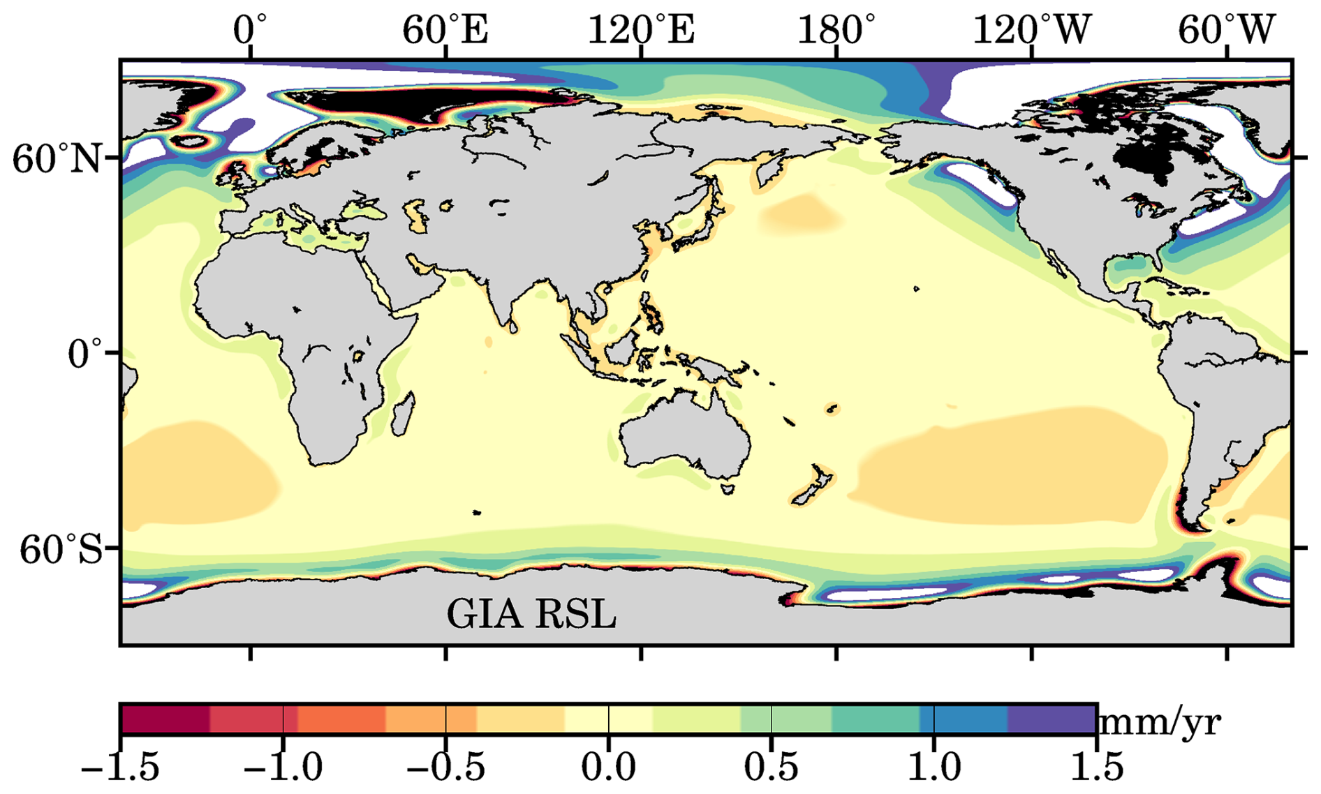
Figure 6 Rate of relative sea level predicted by the model ICE-6G_C (Peltier et al., 2015).

2.7 Sea level reconstructions from previous studies

In this study, our sea level reconstructions are evaluated against publicly available GMSL reconstructions that have been widely used in sea level studies. These community-accessible GMSL reconstructions are based on various approaches and incorporate different considerations of tide gauges (Table 2). By comparing this study [M2025] to these reconstructions, we show our major advantage, i.e., complete and publicly available time series at the exact sites of tide gauges, which motivates this paper.

Both Church and White (2011) [C2011] and Ray and Douglas (2011) [R2011] employed the classic EOF reconstruction technique. R2011 considered the smallest number of tide gauges with annual records and resolved the datums for tide gauges. Jevrejeva et al. (2014) [J2014] reconstructed the longest records for GMSL with the largest numbers of tide gauges using the station stacking method. Hay et al. (2015) [H2015] initiated the data assimilation approach by incorporating 622 tide gauges. Their work inspires this study. These four reconstructions delivered fundamental time series for GMSL, but not for local stations.

There are correlations among the reconstructions by Dangendorf et al. (2019) [D2019], Frederikse et al. (2020) [F2020], Dangendorf et al. (2024) [D2024], Treu et al. (2024) [T2024], and M2025. Figure 7 illustrates their dependency or genetic relation. The hybrid reconstruction by D2019 combined the data assimilation and EOF techniques to capture both long-term trends and interannual variability. Note that D2019 inherited the outputs of the data assimilation by H2015, and T2024 adopted low-frequency changes from D2019. F2020 used the station stacking method to compute the GMSL for 1900–2018, and more importantly, F2020 diagnosed the sea level budget for global mean and basin mean, with consideration of SLF described in Sect. 2.5. The SLF computed by F2020 is incorporated by D2024 and M2025. Both D2024 and M2025 improved the data assimilation approach based on H2015. Specifically, [D2024] developed a novel data assimilation approach that resolves spatial variability in sea level changes. This study introduces the random process to improve the performance of CMIP6 models at local scale (see Sect. 3.4).

Table 2 Overview of sea level reconstruction studies.

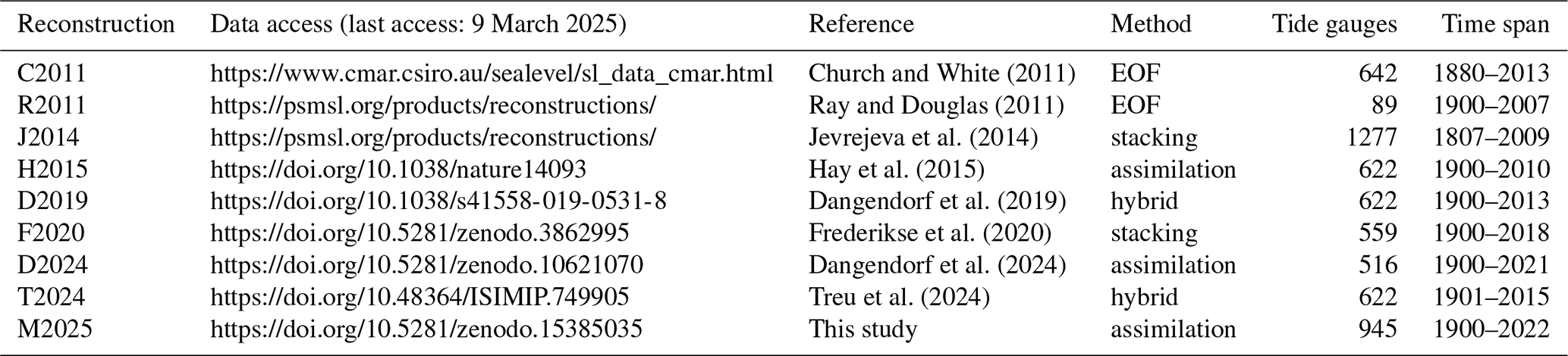
A particular comparison should be highlighted between T2024 and M2025. Table 3 summarizes main features (pros and cons) in T2024 and M2025The key feature of T2024 is that they synthesized sea level rise at local scale by integrating several different datasets. Their low-frequency relative sea level changes (mainly reflecting sea level trends) are extracted from the combination of D2019 and Oelsmann et al. (2024). The former provides the geocentric sea level, and the latter releases the vertical land motion. The difference between those two variables defines the relative sea level, which is also reconstructed by M2025.

Table 3 Comparisons of sea level reconstruction by T2024 and M2025.

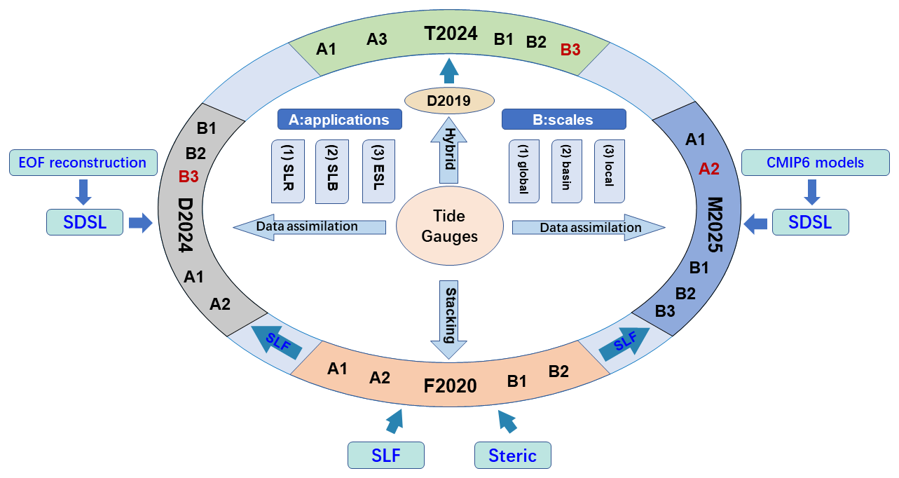
Figure 7 Relation among the reconstructions by D2019, F2020, D2024, T2024, and M2025. A (applications) and B (scales) indicate their suitable investigations at various spatial scales, for example, A1 means the reconstruction can be used for the sea level rise, and B2 means it can be suitable for basin scale. Colour red (e.g., A2 or B3) means there are limitations. SLR = sea level rise; SLB = sea level budget; ESL = extreme sea level.

T2024 adopted an irregular grid covering global coast. If the sea level reconstruction by D2019 is not available at locations of this grid, T2024 interpolated or extrapolated the sea level based on D2019 grid. In addition, the reconstruction by D2019 employed projection from the locations of tide gauges onto the satellite altimetry grid, which means D2019 does not directly cover the sites of tide gauges. We therefore must stress that the sea level reconstruction by T2024 is not built on the exact sites of tide gauges, which is a major difference from M2025. An apparent advantage in T2024 is that they include high frequency variability in the reconstructed sea level time series. They released monthly reconstructions for 1901–1978, and hourly reconstructions for 1979–2015. However, our reconstructions do not contain high frequency sea level variability, which is a major limitation (see Sect. 4).

For application purpose, we further summarize their suitability for the study of sea level rise. First, all the reconstructions shown in Table 2 allow for quantifying the GMSL rise over the twentieth century. Both F2020 and D2024 enable community to investigate sea level budget at global and basin scale. D2024, T2024, and M2025 released sea levels along coasts, but only M2025 builds reconstructions at the sites of tide gauges. D2024 and T2024 involve either extrapolations or locations merging; therefore, investigation of local sea level rise should be interpreted with cautions.

2.8 Satellite altimetry

We use monthly sea level time series provided by Archiving, Validation and Interpretation of Satellite Oceanographic (AVISO) service (https://www.aviso.altimetry.fr/en/home.html, last access: 9 March 2025). This product is spatially gridded into a 0.25° × 0.25° grid, which combines measurements from TOPEX/Poseidon, Jason-1/2/3, HY-2, Sentinel-3A, and Cryosat-2. Various geophysical corrections (e.g., Yuan et al., 2021), e.g., wet troposphere correction, and atmospheric loading correction, have been applied to the AVISO grids. In addition to the gridded monthly products, AVISO also releases weekly GMSL time series that have been corrected for GIA effect. The time series are available at https://data.aviso.altimetry.fr/aviso-gateway/data/indicators/msl/ (last access: 9 March 2025). The weekly data are averaged to annual time series. Both the AVISO gridded product and its GMSL time series are compared to our sea level reconstructions.

2.9 Ocean reanalysis

To quantify the performance of CMIP6 climate models at local scale, we consider the SDSL time series from Ocean Reanalysis System 5 (ORAS5; Zuo et al., 2019). The ORAS5 dataset is produced by European Centre for Medium-Range Weather Forecasts and funded by the Copernicus Climate Change Service. This reanalysis combines model data with observations from across the world into a globally consistent dataset with accounting for the laws of physics. The ORAS5 data is forced by either global atmospheric reanalysis (for the consolidated product) or operational analysis (for the operational product) and is also constrained by observational data of sea surface temperature, sea surface salinity, sea-ice concentration, global-mean-sea-level trends and climatological variations of the ocean mass. We employ the consolidated product spanning period 1958–2014.

2.10 Validation methodology

Our sea level reconstructions are validated through comparing with sea level observations and other sea level reconstructions. The validation process includes comparisons at global and local scales. At global scale, sea level reconstructions are commonly compared to the sea level rise observed by satellite altimetry, because it provides robust evidence for the GMSL rise. At selected locations, our reconstructions are compared to AVISO sea level products. We use the AVISO time series to implement the comparison over 1993–2022, which means a limited period for comparison. To validate our sea level reconstructions over the twentieth century, we compare them with other sea level reconstructions. Several reconstructed GMSL time series are publicly available (Table 2), those sea level reconstructions are considered for the validation at global scale. Sea level reconstructions are valuable at local scale, but they are less available. T2024 addressed this issue, and their sea level reconstruction offers an independent estimate for validating our sea level reconstruction. We average their monthly and hourly reconstructions into yearly time series, consistent with our reconstructions. However, as mentioned in Sect. 2.7, T2024 reconstruction was performed on a coastal grid by interpolating or extrapolating the reconstruction by D2019, they do not directly provide time series at the exact sites of tide gauges. To implement the comparison, we select the nearest grid point from T2024 for each tide gauge site considered in this study.

3 Results

In this section, we present the main results, beginning with several examples of sea level reconstruction at different tide gauges that illustrate the diversity in reconstructions. They are followed by comparisons between our reconstructions and other estimates, including observations from satellite altimetry and other sea level reconstructions. Those comparisons serve to verify our reconstruction at global and local scales, and elaborate the merits and limitations in our reconstructions. The final subsection is dedicated to addressing the statistical assessments, e.g., spread, median, or a particular percentile.

3.1 Examples of sea level reconstruction

Figure 8 plots reconstructed sea level time series at four selected tide gauges. These examples highlight the presence of substantial data gaps over 1900–2022. For instance, Daugavgriva, station ID 37, ceased to record sea level since 1940 (Fig. 8a). Dunkerque, station ID 468, started to observe sea level since around 1950 (Fig. 8c), but it is also associated with a data gap from 1980 to 2000. Sokcho, station ID 1365, only covered a short time duration (Fig. 8d). Our sea level reconstructions fill in those gaps, regardless of their duration. More importantly, our reconstructions are physical interpolations/extrapolations, because they accommodate simulated sea level from climate models and predicted sea level owing to water exchange between land and oceans (i.e., the GRD effect).

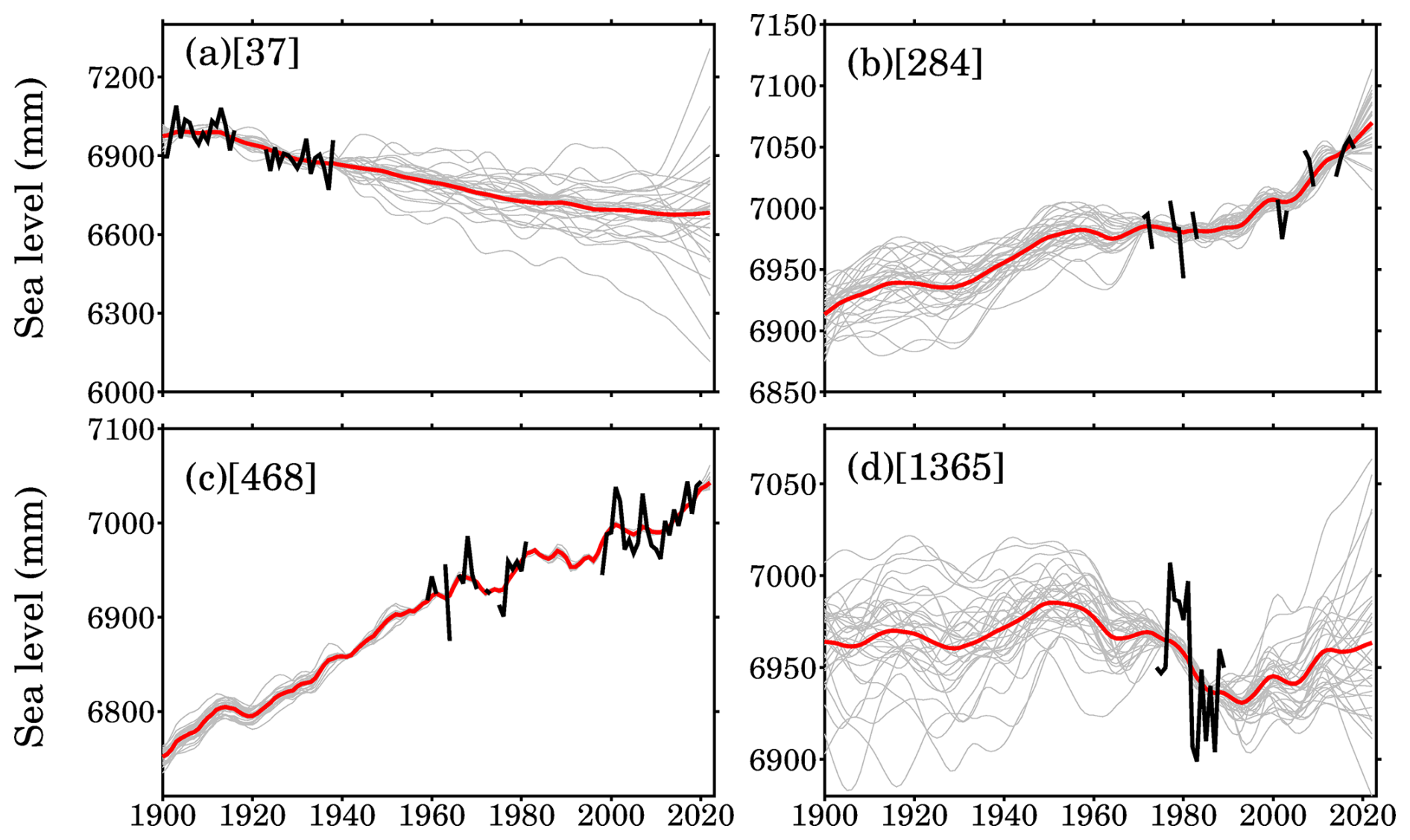
Figure 8 Examples of sea level reconstructions at selected tide gauges. (a) Daugavgriva, PSMSL ID 37; (b) Durban, PSMSL ID 284; (c) Dunkerque, PSMSL ID 468; (d) Sokcho, PSMSL ID 1365. Black lines are raw records from PSMSL; gray lines are individual reconstructions derived with 35 climate models using our assimilation framework at the same locations of tide gauges; red lines represent the ensemble mean.

Two notable features emerge from our sea level reconstructions. First, the 35 reconstructed sea level time series are characterized by smooth and refined curves with reduced year-to-year fluctuations compared to the raw tide gauge records (Fig. 8). Second, the 35 reconstructed time series converge when raw records are available, underscoring the strong influence of sea level observations on constraining the reconstructions. In contrast, in the absence of observations (i.e., during data gaps), the reconstructions exhibit a wider range of behaviours, reflecting the inherent spread among climate model simulations at local scales. In some cases, such as Fig. 6a, the spread in the reconstructed sea level at the final time step (year 2022) can approach 1 m. The average of all 35 reconstructed curves, i.e., the red lines shown in Fig. 8, suggests smoother and more refined sea level changes at tide gauges. This feature is expected, because the average tends to reduce variations across the ensemble.

3.2 Comparison with other estimates

3.2.1 Comparison with satellite altimetry

We first compare our reconstructions with observations from satellite altimetry (Fig. 9a). The average of the 35 GMSL reconstructions based on all 945 tide gauges yields a long-term trend of 3.52 mm yr⁻¹ over 1993–2022, highly consistent with the trend (3.56 mm yr⁻¹) of the GMSL observed by satellite altimetry. However, this apparent consistency should be interpreted with caution, as it may involve differences in definitions of GMSL, inherent uncertainties, and coincidental agreement. First, although both our sea level reconstructions and satellite observations are corrected for GIA effect, they represent fundamentally different quantities: our reconstruction reflects relative sea level at tide gauge locations, while satellite altimetry measures absolute sea level over the global oceans. Secondly, our reconstructions represent very limited samples of changes in sea level along coastal zone, it does not include any changes in the ocean interior, although it does cover high latitudes, where are not observed by satellite altimetry.

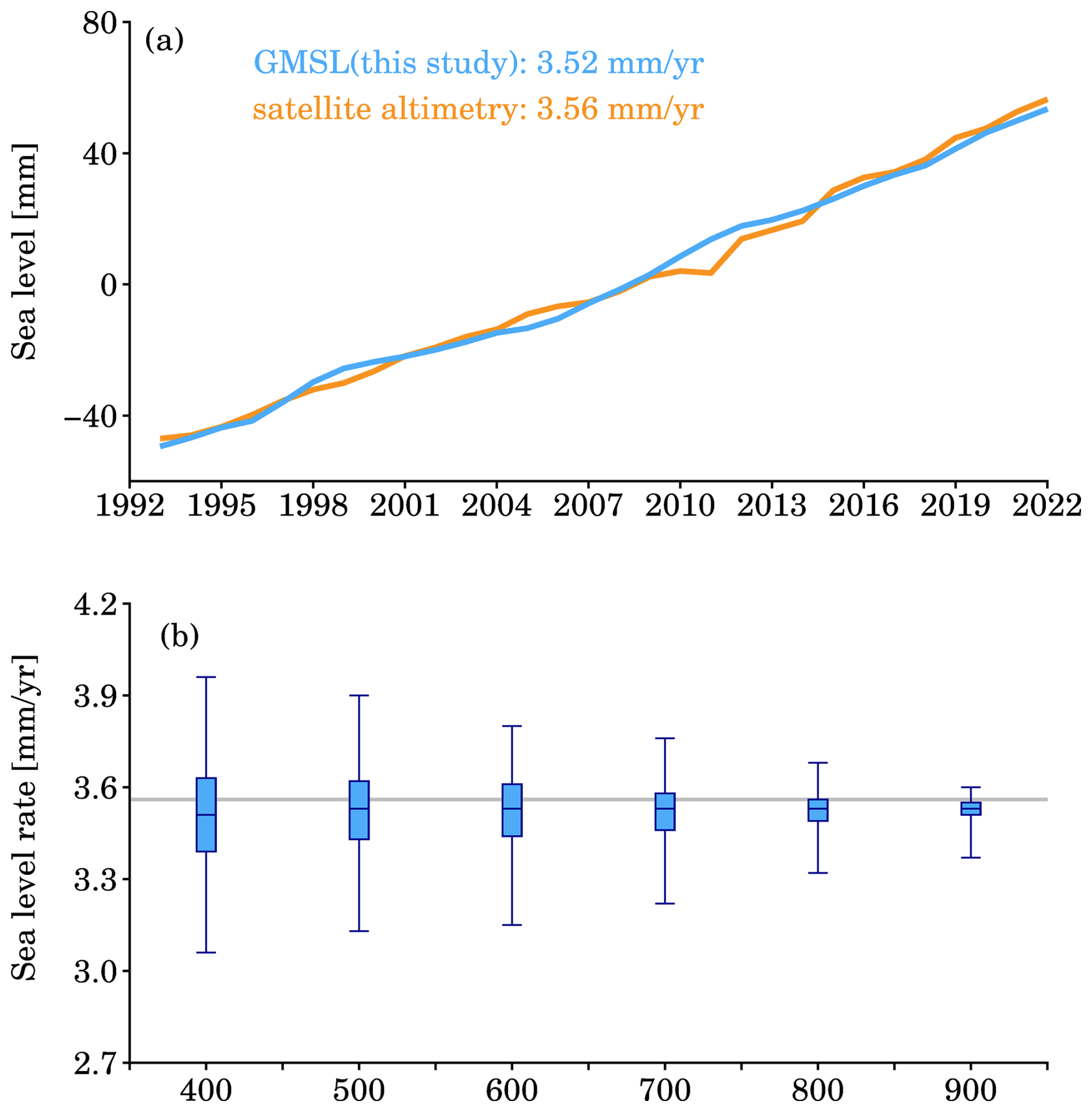
Figure 9 Global mean sea level (GMSL) and its rate over 1993–2022. (a) Blue line is the average of 945 tide gauges, and orange line is provided by AVISO (section 2.8); (b) boxplots show ensemble mean rates using different numbers of tide gauges, gray line indicates the GMSL trend from AVISO.

The samples (numbers and distributions) of tide gauges indeed affect the average sea level rates. To evaluate this effect, we extract a subset from the reconstructed sea level at total tide gauges. The ensemble of subsets ranges from 400 to 900 with a 100 interval. For each subset, we randomly repeat the spatial resample for 1000 times, then compute the median (50th percentile), maximum (100th percentile), minimum (0th percentile), and quartiles (25th percentile and 75th percentile). The resulting statistics (Fig. 9b) indicate that a small subset has a wide range between the maximum and minimum. For example, for the subset of 400, the maximum rate is 3.96 mm yr⁻¹, and the minimum rate is 3.06 mm yr⁻¹, yielding a 0.9 mm yr⁻¹ total range. This range is reduced to 0.23 mm yr⁻¹ for the subset of 900. We also note that the median is very close to the GMSL rate from satellite altimetry, regardless the number of subsets.

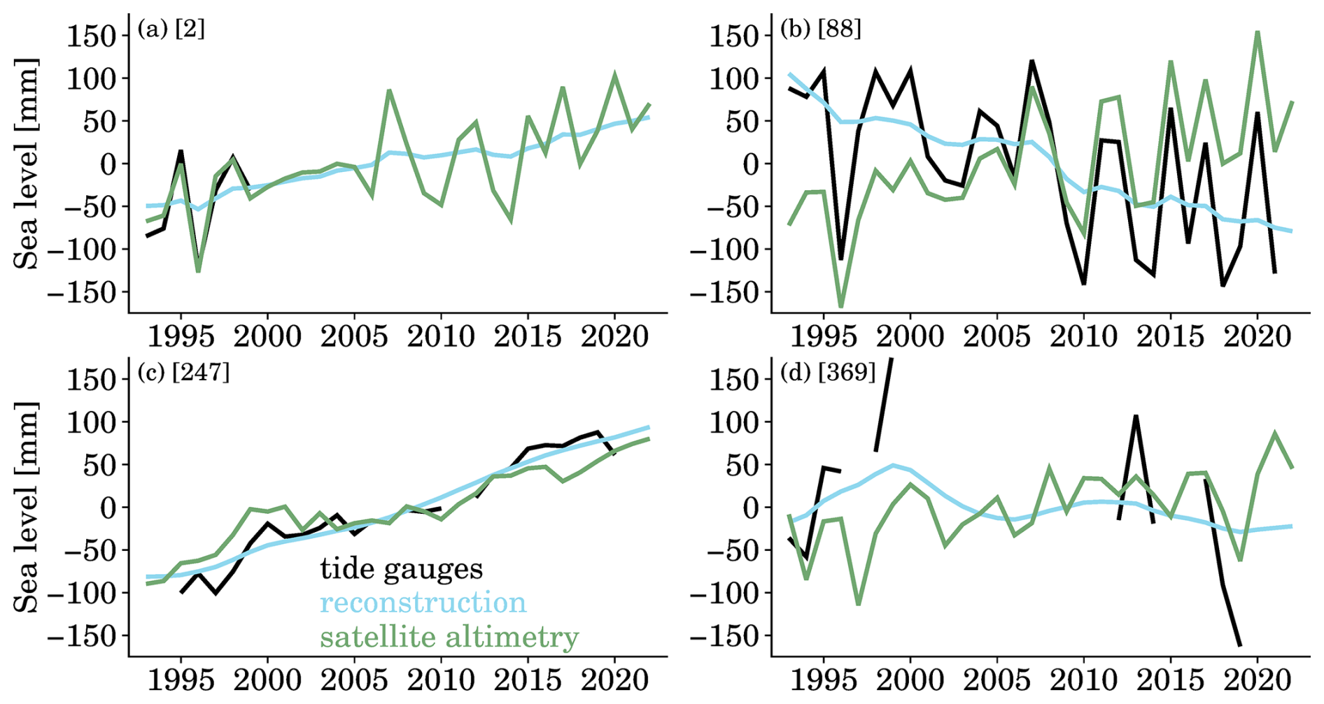
Figure 10 Sea level time series at selected tide gauges. (a) Swinoujscie, PSMSL ID 2; (b) Ratan, PSMSL ID 88; (c) Port Lyttelton, PSMSL ID 247; (d) Garden Reach, PSMSL ID 369. Black lines are raw records from PSMSL, green lines are observed by satellite altimetry, and the blue lines are the average time series reconstructed by this study.

Our sea level reconstructions are also compared against observations from satellite altimetry at some locations. Figure 10 shows the comparisons at four selected tide gauges. The blue lines in Fig. 8 are the average of 35 sea level reconstructions. Since satellite altimetry products usually do not provide direct estimates at the sites of tide gauges, we consider the nearest grid point from AVISO grids within 50 km. At some locations (e.g., Fig. 10a and b), tide gauges exhibit very similar variability to the satellite altimetry, although their trends might be apparently different. The difference in sea level trends could be attributed to several factors. For instance, a major reason is related to the local vertical land motion (Woppelmann and Marcos, 2016), because tide gauges observe relative sea level changes, but the satellite altimetry monitors the absolute sea level changes, variations in local vertical land motion would cause difference in those two observations. Other factors could be related to errors in observations, and local forcing (e.g., Woodworth et al., 2019; Piecuch et al., 2019). We note that, at some sites of tide gauges, our sea level reconstructions agree with the observations from satellite altimetry, even if the records of tide gauges are not available (Fig. 10a and d). However, this agreement is built on the average of reconstructions, there could be larger discrepancies in individual reconstruction (for instance, see Fig. 8).

3.2.2 Comparison with other sea level reconstructions

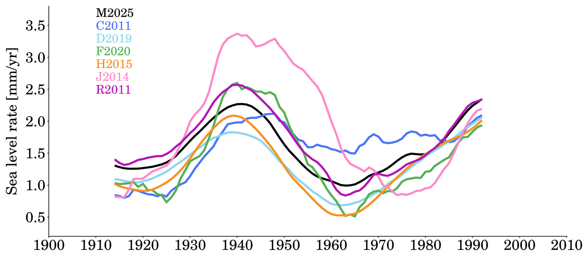
We compare our reconstructions to other sea level reconstructions for the GMSL curves (Fig. 11). When determining the GMSL rate, we consider the period 1900–2007, because this period is commonly covered by all reconstructions. Overall, our reconstructed GMSL curve aligns with other reconstructed GMSL curves, representing a new, independent estimate of GMSL rise. Those curves generate GMSL rates ranging from 1.31 to 1.98 mm yr⁻¹. The highest rate is determined by J2014 who employed a station stacking method. The lowest rate is identified by H2015 who proposed the data assimilation approach. Our curve yields a rate of 1.60 mm yr⁻¹, very close to the rate of 1.62 mm yr⁻¹ by C2011.

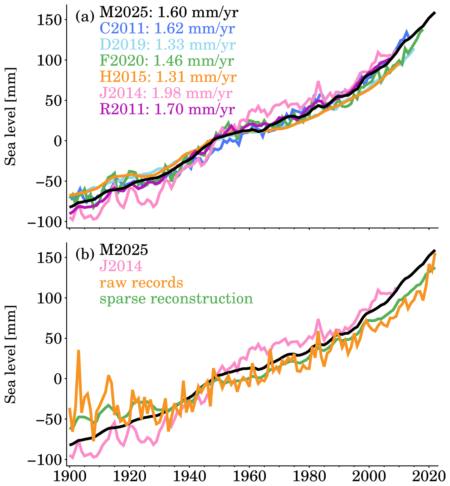
Figure 11 Global mean sea level rise since 1900. (a) compares different sea level reconstructions from this study [M2025], Church and White (2011) [C2011], Ray and Douglas (2011) [R2011], Jevrejeva et al. (2014) [J2014], Dangendorf et al. (2019) [D2019], and Frederikse et al. (2020) [F2020], the rates are estimated for 1900–2007, as this period is covered by all reconstructions. (b) “raw records” is the GMSL that is recomputed with raw records from the tide gauges selected by this paper, “sparse reconstruction” is the GMSL that uses the reconstructed sea level when raw records are available (i.e., with data gaps).

The discrepancies among these reconstructions can be largely attributed to the methodology, but the selection and distribution of tide gauges also plays an important role. For instance, while both C2011 and R2011 employed the classic EOF reconstruction method, they yielded substantially different estimates of GMSL rise (Fig. 11a). This discrepancy primarily stems from the fact that R2011 incorporated only 89 tide gauges, whereas C2011 utilized more than 500 tide gauges (Table 2). The spatial coverage of tide gauges strongly influences the resulting reconstruction, as also demonstrated by our resampling experiment (Fig. 11b) and Hamlington and Thompson (2015). In addition, there is a subtle difference in the GMSL curves shown in Fig. 11b, and this difference concerns the definitions of relative or absolute GMSL (Dangendorf et al., 2017). Some GMSL curves, e.g., C2011 and J2014 represent absolute GMSL rise, at least in theory, because they corrected the tide gauges for vertical land motion, but only accounting for the changes induced by GIA, not the total changes. Other GMSL curves, e.g., H2015 and M2025, reflect relative GMSL rise, as they accounted for the relative sea level rise associated with GIA (see Eq. 1). We can assess the difference between relative GMSL and absolute GMSL using our reconstructed sea levels, or by an alternative approach. To obtain the absolute GMSL, we should account for the vertical land motion associated with GIA, which means absolute GMSL = tide gauges + vertical land motion (GIA); on the other hand, the relative GMSL is derived by “tide gauges – relative sea level (GIA)”. Hence, we only need to compare the vertical land motion (GIA) to −1 × relative sea level (GIA). These two components are computed using the ICE-6G_C model (Peltier et al., 2015), their average at 945 tide gauges are estimated to be 0.23 and −0.38 mm yr⁻¹, yielding a 0.15 mm yr⁻¹ rate difference between our relative GMSL and absolute GMSL.

It is noteworthy that the reconstruction by J2014 shows the largest interannual variability (Fig. 11). We suspect that these fluctuations are caused by direct average from raw records. To test this hypothesis, we construct two additional GMSL time series: one based on the raw tide gauge records, and another based on our reconstruction, restricted to periods when raw records are available (Fig. 11b). The resulting GMSL curves with raw records exhibit large interannual variability, similar to the result of J2014, confirming our conjecture. Interestingly, Fig. 9b also suggests a lower GMSL rise during the early twentieth century (1900–1930) compared to our full reconstruction and that of J2014. This discrepancy may be linked to data gaps (when comparing raw records with our reconstruction) and the smaller number of tide gauges used (when comparing with J2014).

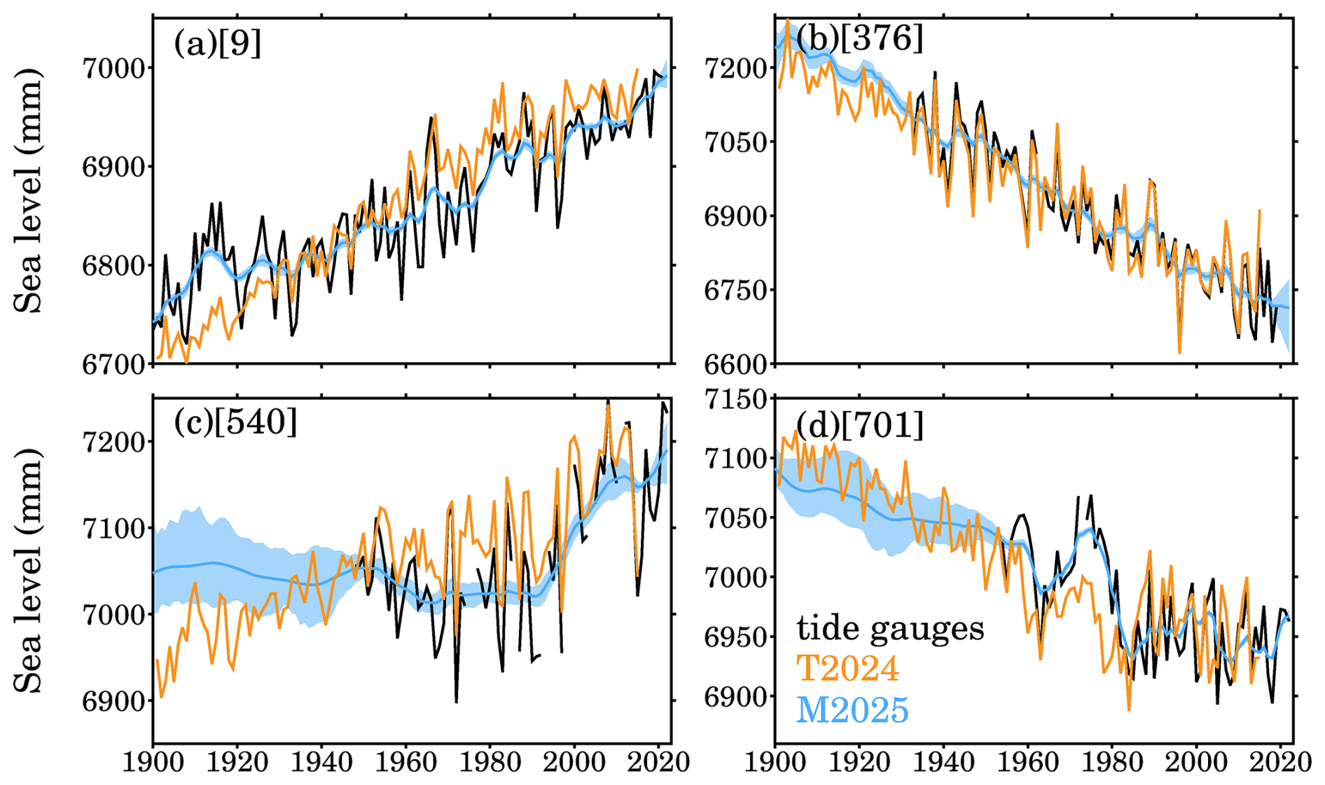
Figure 12 Comparisons of sea level reconstruction at selected tide gauges. (a) Maassluis, PSMSL ID 9; (b) Rauma, PSMSL ID 376; (c) Apra Harbor, PSMSL ID 540; (d) Kainan, PSMSL ID 701. Black lines are raw records from PSMSL, orange lines are reconstructed by Treu et al. (2024) [T2024], blue lines are the medians reconstructed by this study [M2025], and the light blue shading indicates the uncertainty bounded by 10th percentile and 90th percentile.

Our sea level reconstructions at tide gauges are compared to the time series reconstructed by T2024. Figure 12 shows the comparisons at four selected tide gauges. It is clearly noted that the sea level reconstructions by T2024 are associated with high-frequency variations (year-to-year fluctuations), which are also suggested by the raw records, those fluctuations are even highly consistent at some tide gauges, e.g., ID 376 (Fig. 12b). However, there are also apparent discrepancies in low frequency changes, e.g., tide gauges ID 9 and ID 701. Those discrepancies probably originate from the covariance difference between tide gauges and satellite altimetry, as the latter's covariance is used to determine the sea level reconstruction. On the other hand, our sea level reconstructions closely align with the raw records, because in our data assimilation, those raw records are employed to constrain the sea level reconstructions, or in other words, our sea level reconstructions always follow the raw records, underscoring the importance of the observed evidence for sea level rise. From Fig. 12, we observe evident difference between the sea level reconstruction by T2024 and our sea level reconstructions, especially when the raw tide gauges are not available, e.g., Fig. 12c. In those situations, the sea level reconstructions are essentially extrapolated given the reconstruction methods or information, our extrapolations are mainly based on the sea level physics (model simulations and predictions, see Sect. 2 and Table 3), while T2024 relies on the covariance from satellite altimetry.

Figure 13 Sea level rate at tide gauges for 1901–2015. (a) This study, average rate of 35 sea level reconstruction; (b) T2024; (c) difference between this study and T2024; (d) 95th percentile rate of 35 sea level reconstruction; (e) 5th percentile rate of 35 sea level reconstruction; (f) difference between 95th percentile rate and 5th percentile rate.

Different reconstructions may indicate diverse sea level trends. We compute the sea level rates at all tide gauges for 1901–2015 (Fig. 13), and evaluate the rate difference between our sea level reconstruction and the reconstruction by T2024. Note that our sea level rates are computed from the average of the ensemble of sea level reconstructions. The rate comparison suggests that our sea level reconstruction is associated with high spatial variability, for instance, along the Arctic coast, South America coast, and around the Pacific Oceans, on the other hand, the sea level reconstruction by T2024 is characterized with a rather smoothed pattern, especially around the Europe coast (excluding the Baltic Sea), Asia east coast and Australia coast. Indeed, the rate differences are evident along the Arctic coast, the South America coast. We identity a rate of 9.25 mm yr⁻¹ for the maximum difference, and a rate of −7.78 mm yr⁻¹ for the minimum difference. Despite the spatial difference, on average, our sea level rates are surprisingly consistent with the sea level rates by T2024, two datasets generate average rates of 1.22 and 1.20 mm yr⁻¹, respectively, associated with standard deviations of 2.42 and 2.08 mm yr⁻¹, respectively.

Another advantage in our sea level reconstructions is that, unlike the reconstruction by T2024 who provided only a single time series, we provide an ensemble of sea level reconstructions that include 35 time series at each tide gauge (see Fig. 8). We can compute either the average (red lines in Fig. 8) or the median (blue lines in Fig. 12) using those 35 complete time series, and use the average or median to represent the robust sea level reconstruction at tide gauges. We find that at most tide gauges, the average and the median are almost identical (Fig. 13a and e). In addition, the ensemble of our sea level reconstructions permits for the computation of a particular percentile, for example, the 90th and 10th percentiles, and those two percentiles can form boundaries for uncertainties (see the light blue shading in Fig. 12). In the following subsection, we illustrate how to assess the sea level rate using the ensemble of our sea level reconstructions.

3.3 Statistical assessments

In this subsection, we present statistical assessments for sea level rise using our reconstructed time series. Given the ensemble of 35 sea level reconstructions (see Fig. 8 for examples), we can compute average, spread, median, or a particular percentile for both sea level rates and sea level curves. For instance, Fig. 8c shows 35 sea level reconstructions at tide gauge Durban, PSMSL ID 284. For each sea level reconstruction (or curve), we can compute a linear rate (or acceleration) over a period of interest. Figure 14 plots 35 sea level rate over 1900–2022 at tide gauge Durban for all sea level reconstructions. Those 35 rates range from 0.70 mm yr⁻¹ (minimum, or 0th percentile) to 1.38 mm yr⁻¹ (maximum, or 100th percentile), with a median rate of 0.95 mm yr⁻¹, which is very close to the average rate of 0.97 mm yr⁻¹, as shown in Fig. 14. There are two ways to estimate the uncertainty for the rate. We can compute the spread (i.e., standard deviation) using those 35 rates, or alternatively, we can compute percentiles (e.g., 10th and 90th) to form boundaries for the rate uncertainty (see Fig. 14). At most tide gauges, we report that the rate differences are generally small (< 0.1 mm yr⁻¹, see Fig. 13) between the median and the average, although several tide gauges are identified to have high value of rate differences (> 5 mm yr⁻¹), because they have large abrupt jumps (see Sect. 4) that affects the sea level reconstructions.

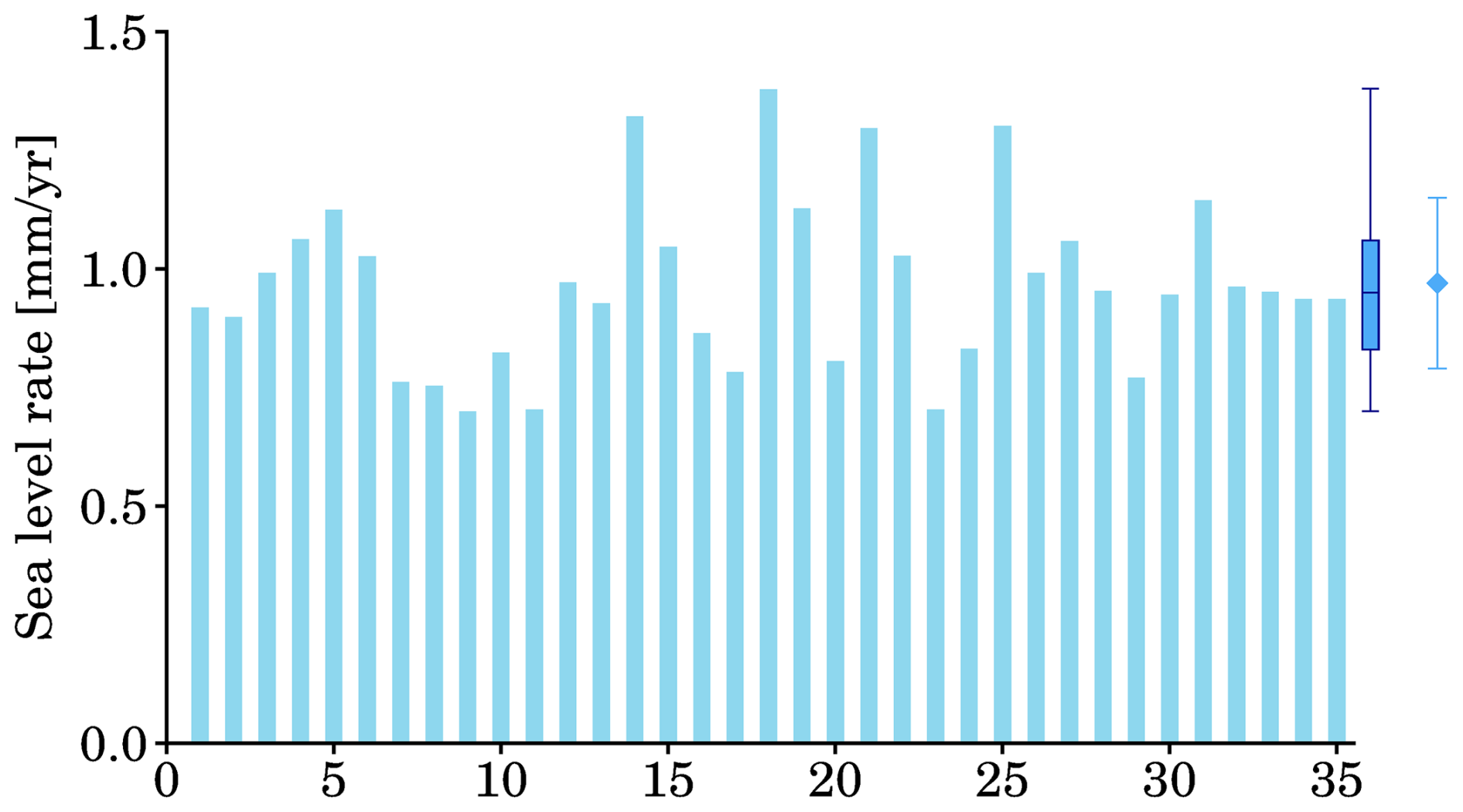
Figure 14 Sea level rate over 1900–2022 at tide gauge Durban, PSMSL ID 284. The 35 thin rectangles represent sea level rates estimated from our 35 sea level reconstructions with climate models (see model index in Table 1), the 35 curves are shown in Fig. 6b; the boxplot on the right side indicates the 0th, 25th, 50th (median), 75th, and 100th percentiles, the diamond on the right side indicates the average rate and the error bar indicates the spread (i.e., standard deviation), the median rate is almost identical to the average rate.

The rate spreads at tide gauges are demonstrated to be time-variable. We explore the rate spreads for two periods, 1900–2020 and 1900–1950 (Fig. 15). Over these two periods, large spreads (> 0.8 mm yr⁻¹) are mainly shown along Arctic coast, which are primarily attributed to the diversity in the SDSL changes. We also note that the spreads over 1900–1950 are larger than the spreads over 1900–2020, a major reason is that sea level rate estimates are more variable over short periods, resulting in large spreads. Small spreads (< 0.4 mm yr⁻¹) are observed along the coast of India, North America, and Europe. Those small spreads are either caused by similar sea level reconstructions or small trends in sea level rise. In the former cases, raw records are available at most time points, leading to very similar reconstructions (see Fig. 12a), as our sea level reconstructions closely follow raw records.

Figure 15 Spread in sea level rate at tide gauges. (a) 1900–2020; (b) 1900–1950.

We stress that the spread shown in Figs. 14 and 15 only reflect the degree of inherent consistency among the reconstructed sea levels, or model/reconstruction diversity. It is very likely that the spread underestimates the true uncertainty, because it does not include uncertainties due to, e.g., measurements error, GIA modelling error. For example, Church et al. (2004) assumed a 4 mm measurements error for monthly records of tide gauges. They consistently applied this 4 mm error to all tide gauges, hence, resulting in a homogeneous spatial pattern, despite the fact that errors in tide gauges vary sites by sites. Users can further account for this error when they determine the sea level trends from our sea level reconstruction. Studies have shown that the choices of mantle viscosity and lithosphere thickness affect the outputs of GIA models, even under the same ice history (Hay et al., 2013, 2015). However, at the moment, only limited GIA models are available to us, we therefore omit the evaluation of GIA uncertainty.

3.4 Assessments of the random process

To assess the improvement by the random process, we compare the original SDSL from CMIP6 climate models and the SDSL estimated by our data assimilation to ocean reanalysis ORAS5. The estimated SDSL consists of the original SDSL plus the random process. Note that original global mean of ORAS5 should be removed, as it does not properly represent the real global mean of SDSL. After this removal, we add the CMIP6 global mean (shown in Fig. 3) to ORAS5; this means we have 35 ORAS5 SDSL, which are compared to either 35 original SDSL from CMIP6 climate model or 35 estimated SDSL. The comparison is implemented using pair-to-pair sea level rates at tide gauges. On average (Fig. 16), the correlations among the SDSL rates are very low. It is −0.05 between original CMIP6 SDSL and ORAS5 SDSL, and it is improved to be 0.14 between the estimated SDSL and ORAS5 SDSL. Despite this weak correlation, it should prove the useful help from the introduction of the random process.

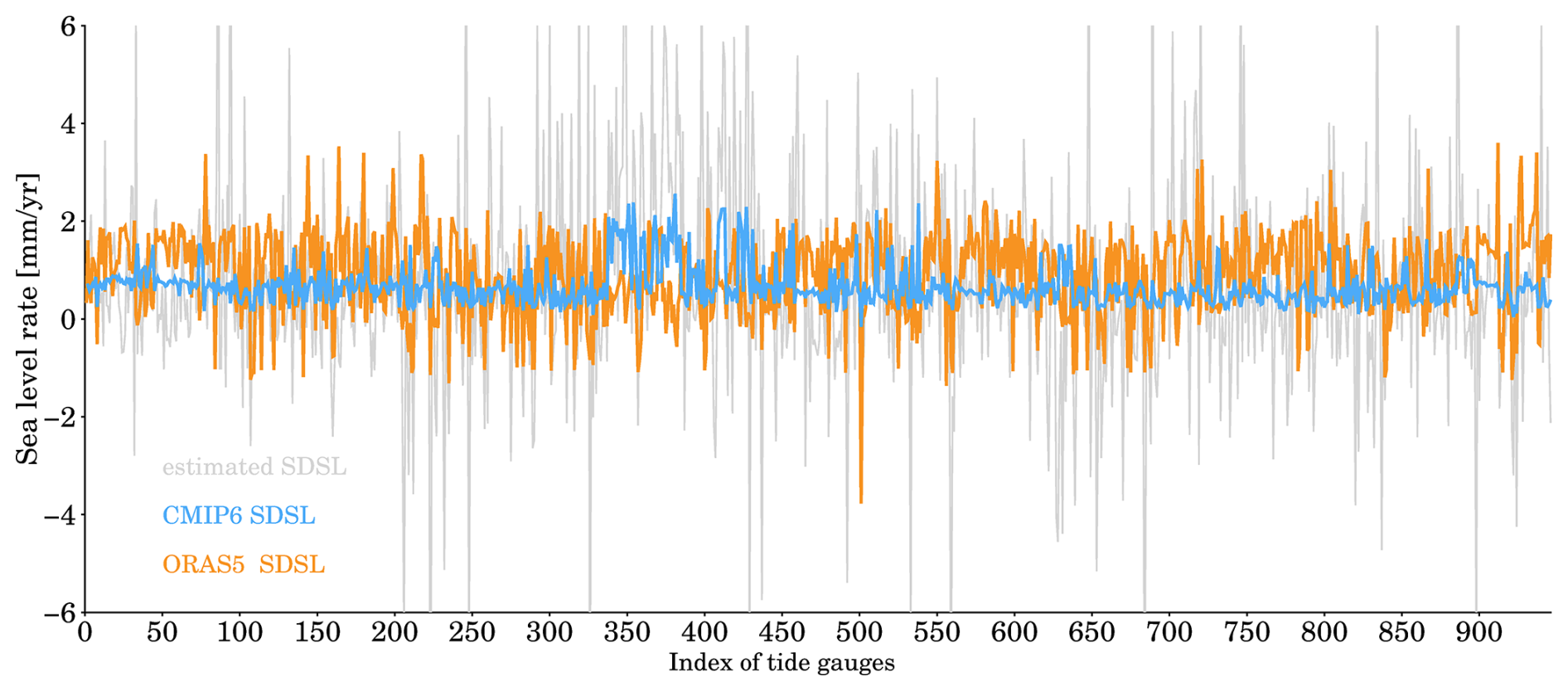
Figure 16 Sterodynamic sea level (SDSL) rates at 945 tide gauges. Blue line is the raw SDSL from CMIP6 (mean of 35 models), orange line is from ORAS5, and gray line is estimated by our data assimilation (i.e., raw CMIP6 SDSL + random process).

We assess the agreements for individual CMIP6 model. We find that some CMIP6 models show correlations with larger values if we use their original SDSL. The strongest correlation (0.51) is produced by model NorESM2-MM (No. 33 shown in Table 1), followed by BCC-ESM1 (0.31), CanESM5-1 (0.43), CMCC-CM2-HR4 (0.34), CMCC-ESM2 (0.39), EC-Earth3-Veg (0.35), HadGEM3-GC31-LL (0.39). However, introducing the random process reduces the correlations. In the meanwhile, we find that 21 CMIP6 climate models have correlations weaker than the average if their original SDSL changes are used. This analysis suggest that the random process can improve the SDSL estimates for the majority of CMIP6 models, but also compromise the SDSL behaviour for some models.

We observe that our estimated SDSL have very large rates at many tide gauges. Our explanation is that these tide gauges are associated with data gaps, even substantial ones in some sites. Over the period with gaps, the random process tends to spread, as there are no constraints from observations. The spreads in the random process and the original CMIP6 SDSL essentially form the uncertainty range. We should point out that there are also spreads in the estimated SLFs, but these spreads are relatively smaller. Hence, the total spreads are mainly caused by the spreads in the random process and the original CMIP6 SDSL.

We note that, at many tide gauges, our estimated SDSL have very large rates, larger than ORAS5 and CMIP6. We suspect that both ORAS5 and CMIP6 (tend to) underestimate the sea level rise at tide gauges. To prove this conjecture, we compare two reconstructions to tide gauges, see Fig. 17. The first reconstruction is the average of our sea level reconstruction (by data assimilation), and the second reconstruction is computed using the sea level fingerprints + ORAS5 SDSL + GIA (relative sea level). To estimate robust trends for tide gauges, we only consider tide gauges have valid records > 40 years over 1958–2014, this gives us 350 tide gauges. We can see that our reconstruction closely aligns with the tide gauges, their standard deviations are consistent (3.4 mm yr⁻¹ VS 3.3 mm yr⁻¹); but the reconstruction with ORAS5 underestimates the sea level rise (with a standard deviation of 2.4 mm yr⁻¹), confirming our conjecture.

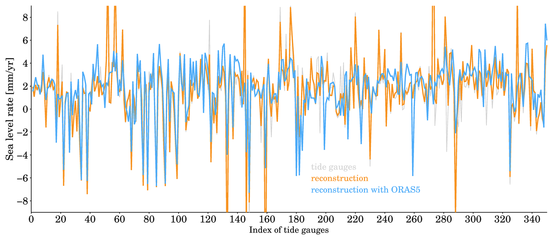
Figure 17 Sea level rates at selected tide gauges. We select tide gauges that have valid records > 40 years over 1958–2014, so their linear trends can be robustly estimated. Orange line is our sea level reconstruction by the data assimilation, and blue line is reconstructed with the combination of ORAS5 SDSL and our estimated SLFs. The 350 tide gauges yield a standard deviation of 3.4 mm yr⁻¹, our reconstruction shows a standard deviation of 3.3 mm yr⁻¹, and the reconstruction with ORAS5 shows a standard deviation of 2.4 mm yr⁻¹.

4 Caveats

Our sea level reconstructions offer complete sea level time series, however, it should be used with caution. They do not purely reflect sea level signals associated with the mechanisms defined in Sect. 2.1, but also possibly contain some changes due to other geophysical processes or anthropogenic activities. It is well known that earthquakes cause abrupt jumps in the records of tide gauges (e.g., Oelsmann et al., 2024). For instance, the tide gauge Ofunato II (PSMSL ID 1364, located in Japan), recorded an abrupt uplift in sea level since 2011, amounting to about 680 mm (Fig. 18). This sudden jump was clearly not caused by SDSL or SLF changes, but actually triggered by the Tohoku-Oki 2011 earthquake (Ozawa et al., 2011; Simons et al., 2011), which resulted in dramatic co-seismic displacement (downward) that consequentially elevated the relative sea level. We also discover an evident decrease in sea level after that jump, which is also not directly attributable to SDSL or SLF mechanisms, but mostly induced by post-seismic uplift, or viscoelastic relaxation (Han et al., 2019) that could persist for years or even decades. There are some similar cases at other tide gauges that experienced uplift or subsidence due to earthquakes. During the process of tide gauges selection, we retain all gauges to maximize spatial coverage. Moreover, the impact of anomalous records is localized and does not significantly affect other stations, although those abnormal records do affect our reconstruction at their tide gauges before and after the sudden jumps. Users should particularly pay attention to those jumps, and inspect the raw records before employing our reconstructions.

A simple approach to identifying the anomalous records is to differentiate the time series from tide gauges. For instance, if the difference between two consecutive time points are larger than 250 mm (Church et al., 2004), then, the records can be treated as anomalies. A more reliable way is to visually inspect the records for all tide gauges. The judgment costs experiences. Among the 945 tide gauges, 13 of them are flagged with issues, based on our own experiences. There PSMSL IDs are: [131; 331; 409; 610; 617; 635; 662; 686; 752; 1061; 1345; 1346; 1364]. We find that excluding these time gauges reduces the GMSL rate from 1.60 to 1.52 mm yr⁻¹ over 1900–2007, indicating a minor effect.

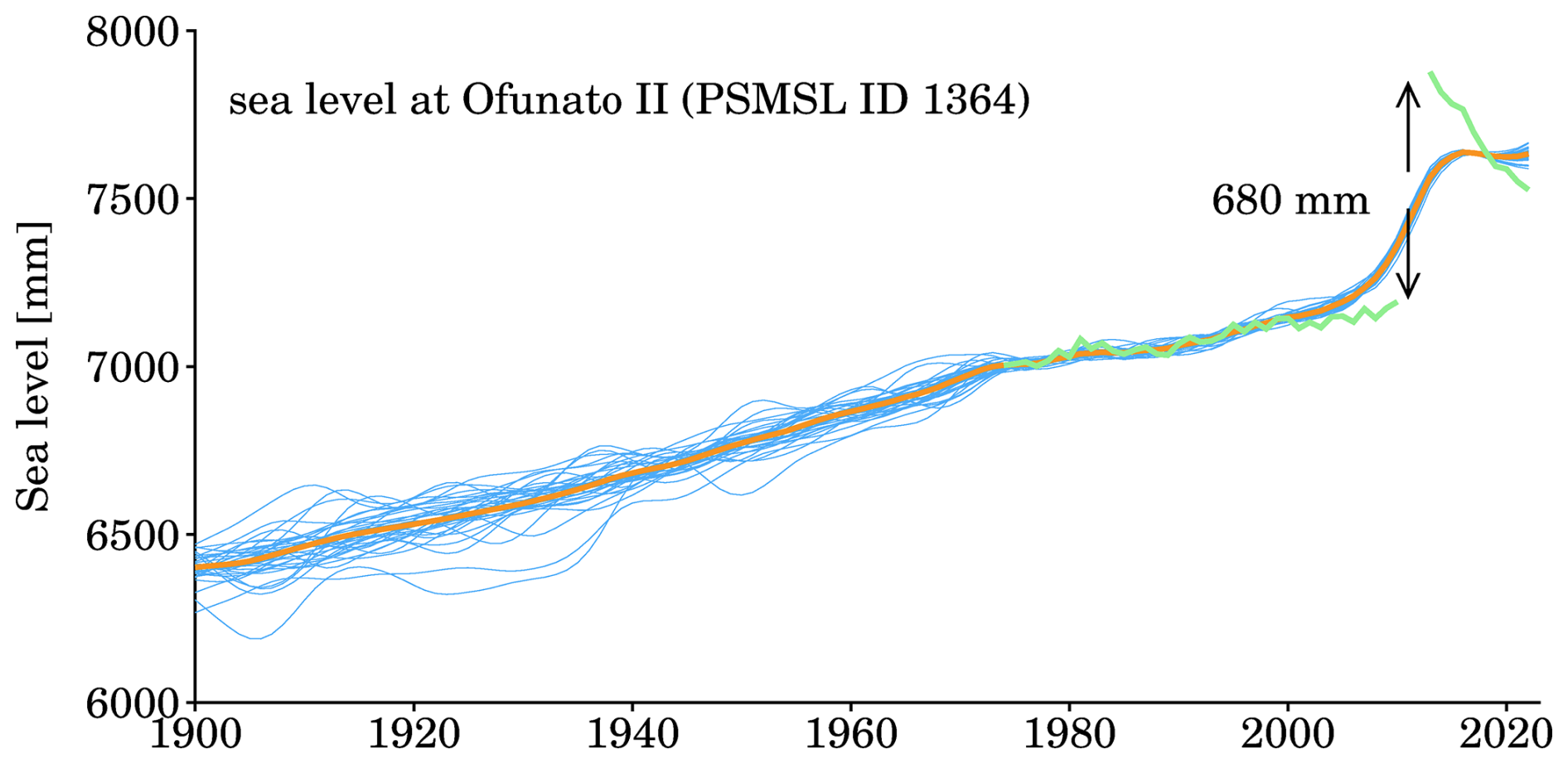
Figure 18 Sea level at tide gauge Ofunato II, PSMSL ID 1364, Japan. Green line is the raw records, which were broken by the 2011 Tohoku-Oki earthquake (Ozawa et al., 2011). This earthquake caused a sudden jump of 680 mm sea level, followed by a rapid decline, which is probably not a sea level signal, but could be mostly attributed to Earth viscoelastic relaxation (e.g., Han et al., 2019). Blue lines are the ensemble of sea level reconstructions, and the orange line is their average. Since the jump is not removed, anomalous jumps are also manifest in our sea level reconstructions.

Our sea level reconstructions are focused on the refined sea level trends, because the data assimilation approach is informed with yearly rates only. The refined trends indeed benefit the study of low-frequency sea level rise, unfortunately, they do not reflect any year-to-year variability as shown in the reconstructions by T2024 (see Fig. 12), and they are probably not suitable for determining trends over a short period. Although the long-term trend and short-term trend may not have an exact diacritical point, we recommend that sea level rates should be estimated over a period larger than 30 years (e.g., Frederikse et al., 2020; Wang et al., 2024). Sea level rates estimated over periods shorter than 30 years should be interpreted cautiously, and their uncertainty might be greatly larger than the spread advised by our sea level reconstructions.

Figure 19 plots the GMSL rate using a 30-year running window. The curve of our GMSL rates fall between other curves, except for the beginning period (1915–1928) and the ending period (1980–1993); over these two periods, our curve lies at the upper bound. The curve of J2014 is apparently distinct from other curves, especially since 1930, this distinction is directly connected with the selection of tide gauges, which is an important factor that affects reconstruction. This can be further confirmed by the difference between C2011 and R2011, especially over 1950–1980; both studies employed the EOF reconstruction, but they used very different distributions of tide gauges, R2011 used only 89 tide gauges, the lowest number for sea level reconstruction considered in this study. We stress that the reconstruction methods also matter, which is demonstrated by the difference between C2015 and D2019, as they considered very similar distribution of tide gauges, D2019 adopted the trends from C2015, but D2019 reconstructed interannual variability with the EOF reconstruction. This difference also implies that the interannual variability has some noticeable effect on the 30-year running rates. A very similar comparison is suggested by Wang et al. (2024), see their Fig. 6.

Figure 19 Global mean sea level rate computed with a 30-year running window.

5 Code and data availability

The released data “SLRv2.nc” from our assimilation framework in this study can be accessed at: https://doi.org/10.5281/zenodo.15385035 (Mu, 2025). It contains the following variables:

• ID: it is a variable with dimension 945 × 1, which contains the ID assigned by PSMSL.

• lon: it is a variable with dimension 945 × 1, which contains the longitude of each tide gauge.

• lat: it is a variable with dimension 945 × 1, which contains the latitude of each tide gauge.

• -year: it is a variable with dimension 123 × 1, the year from 1900 to 2022.

• sea_level: it is a variable with dimension 945 × 123 × 35, which contains the sea level reconstructions at all tide gauges over 1900–2022 for all 35 CMIP6 models.

• RSL: it is a variable with dimension 945 × 1, which contains the GIA relative sea level rates at all tide gauges.

• raw_records: it is a variable with dimension 945 × 123, which contains the annual records from PSMSL. Note that the missing values are denoted by “NaN”.

• average: it is a variable with dimension 945 × 123, which contains the average of sea level reconstructions at all tide gauges over 1900–2022.

• spread: it is a variable with dimension 945 × 123, which contains the ensemble spread (standard deviation) across models at all tide gauges over 1900–2022.

• GMSL: it is variable with dimension 123 × 1, which contains the global average time series of our sea level reconstructions at 945 tide gauges. Note that GIA RSL effect is removed.

• GMSL_spread: it is variable with dimension 123 × 1, which contains the spread of GMSL.

Our data assimilation was run with an open software SSpace (Villegas and Pedregal, 2018), which can be downloaded from: https://doi.org/10.18637/jss.v087.i05. The scripts are only available upon request to Dapeng Mu (mdp321@126.com).

6 Conclusions

In this paper, we reconstructed sea level rise at global 945 tide gauges for 1900–2022 with a data assimilation approach (Hay et al., 2013; Mu et al., 2024a). This approach accommodates sea level simulations from climate models and sea level predictions with the GRD effects (Frederikse et al., 2016), therefore, the resulting sea level reconstructions are physical interpolations and extrapolations. More importantly, by incorporating outputs from 35 climate models, the sea level reconstructions provide refined, continuous time series at tide gauges, and allow for direct uncertainty assessments that reflect reconstruction diversity or probability.

Global comparisons suggest that our sea level reconstructions align with observations and other reconstructions, demonstrating that our sea level reconstructions contribute to the ensemble of reconstructed GMSL curves that are available to the community. In addition to exploring GMSL rise and acceleration, our GMSL time series can serve to validate other reconstructions, and estimate uncertainties. Local comparison with an independent reconstruction by T2024 indicates that our sea level reconstructions closely follow the raw records of tide gauges, signifying that our reconstructions emphasize the importance of the observed evidence. Despite some trend differences from the reconstruction by T2024, our reconstructions are expected to support efforts to understand global sea level rise and its interplay with climate change.