Deep convection life cycle characteristics: a database from the GoAmazon experiment

The Observations and Modeling of the Green Ocean Amazon (GoAmazon2014/5) experiment provided a comprehensive suite of cloud–aerosol–precipitation observations with both in situ and remote-sensing instruments. In this study, we apply a tracking methodology to volumetric radar data, creating a refined database focused on deep convective systems with a full life cycle, incorporating lightning data. This refined deep convection database is shown to be a robust sample of the complete dataset in terms of convective system morphology. The analysis reveals significant seasonal and diurnal variations in convective morphology and intensity, with most intense systems occurring during the dry-season–wet-season transition. The filtered dataset offers a robust sample for future studies on Amazonian convection. The database is available at https://doi.org/10.5281/zenodo.13732692 (Lopes, 2024).

1 Introduction

Due to its large territorial extent that includes pristine forest, agricultural regions, and a large urban zone with an industrial center, the Amazon tropical rainforest serves as a natural test bed for studies on cloud–aerosol–precipitation and land–atmosphere interactions. This complex ecosystem is one of the main centers of convection regulating the climate (Nobre et al., 2009; Artaxo et al., 2022) and the South American monsoon system (SAMS) (Zhou and Lau, 1998; Jones and Carvalho, 2002). Several convection patterns are present in the region, mainly modulated by the Hadley circulation and the corresponding position of the Intertropical Convergence Zone (ITCZ), which determines the Amazonian wet (austral summer) and dry (austral winter) seasons.

Several field experiments have been conducted in the region in order to study different aspects of cloud–aerosol–precipitation interactions in the Amazon. The Amazon Boundary Layer Experiment campaigns ABLE 2A (Harriss et al., 1988) and 2B (Harriss et al., 1990) focused on the chemistry and dynamics of the lower atmosphere in the dry and wet seasons, respectively. The Large-Scale Biosphere–Atmosphere Experiment in Amazonia (LBA) program (Silva Dias et al., 2002) was responsible for numerous field experiments during late 1990s and early 2000s, including the first major mesoscale atmospheric campaign as part of the Tropical Rainfall Measuring Mission (TRMM) validation campaigns and the CHUVA (Cloud Processes of the Main Precipitation Systems in Brazil) project, a contribution to cloud-resolving modeling and to the Global Precipitation Measurement (GPM) mission (Machado et al., 2014a). The Observations and Modeling of the Green Ocean Amazon (GoAmazon2014/5; Martin et al., 2017) campaign was the first long-term experiment to analyze the effects of the Manaus pollution plume at different experimental sites around Manaus, and it included two intensive operation periods (IOPs) during the wet and dry season. Unlike previous experiments, an operational weather radar, operated by Sistema de Proteção da Amazônia (SIPAM – System for the Protection of the Amazon), was available during GoAmazon, and it enabled coverage of all experimental sites with cloud remote-sensing data at great temporal and spatial resolutions. The main goal of the GoAmazon experiment was to analyze cloud–aerosol–precipitation interactions between the forest and the Manaus metropolitan region, specifically the transformation of air plumes from the pristine forest to the Manaus pollution plumes and their subsequent eastern propagation. The goal of the CHUVA-Manaus experiment was to characterize the convection regimes in the region using remote sensing, with the installation of an X-band radar during the experiment and the establishment of partnerships with CENSIPAM (Centro Gestor e Operacional do Sistema de Proteção da Amazônia – Manager and Operational Center of the System for the Protection of the Amazon) for surface radar data and NASA–JAXA (National Aeronautics and Space Administration–Japan Aerospace Exploration Agency) for satellite radar data from TRMM and GPM.

A few studies, such as Giangrande et al. (2017), Machado et al. (2018), Giangrande et al. (2020), and Biscaro et al. (2021), have provided insight into the convection characteristics during GoAmazon. Each of them use different definitions of cloud features employing different sources of remote-sensing data, and they even diverge with respect to their definition of the wet and dry seasons, thereby making it difficult for other studies to follow a homogeneous methodology of convection measurements, especially those that analyze cloud–aerosol–precipitation interactions. For this reason, this study aims to create a comprehensive database and methodology for convective systems based on radar data that can be used in future studies utilizing GoAmazon data.

2 Materials and methods

2.1 Data

Data sources for this study are the GoAmazon (Martin et al., 2017) and CHUVA-Manaus (Machado et al., 2014b) field experiments that occurred between January 2014 and December 2015 around Manaus, Amazonas. The main site of these experiments, named T3, was located in Manacapuru, Amazonas, Brazil (3.213° S, 60.598° W), about 70 km west of Manaus. A wide range of cloud, precipitation, aerosol, and atmospheric instruments were installed at the site, as part of the ARM (Atmospheric Radiation Measurement) mobile facility AMF1 that took measurements during most of the experiment. Some additional instruments and other sites (shown in Fig. 1 of Martin et al., 2017) took measurements during two intensive operation periods (IOPs), with IOP1 being between 1 February and 31 March 2014 (wet season) and IOP2 being between 15 August and 15 October 2014 (dry season). More details about the campaigns can be found in Martin et al. (2016, 2017).

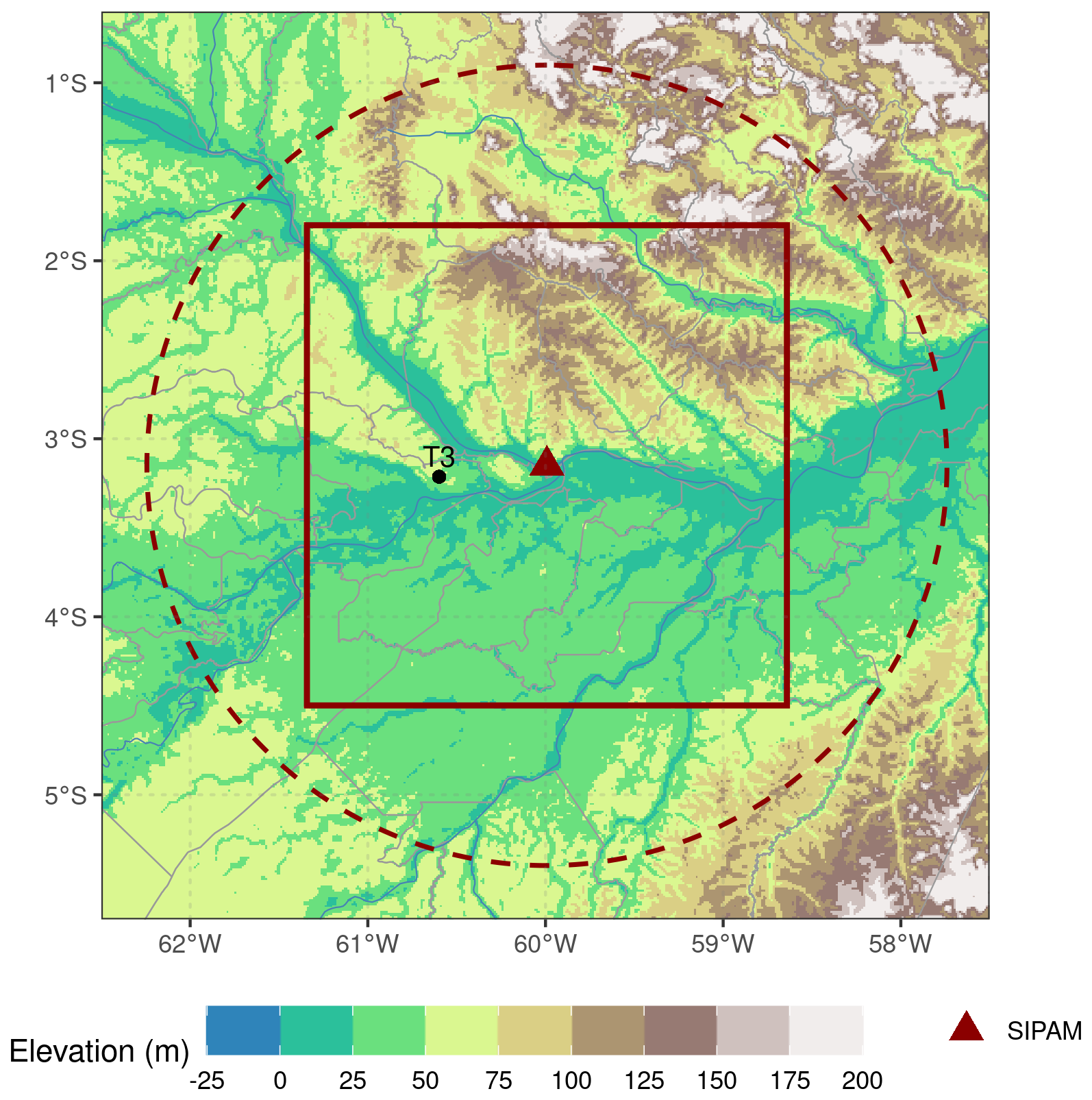
Figure 1 Amazonian region used in this study, showing the SIPAM radar location (red triangle), the 250 km originally calculated coverage (dashed red lines), the 150 km × 150 km bounding box (red square) used in the study, and the T3 site location in Manacapuru where surface data (not shown in this study) were collected.

In order to create the convective system database, radar volumes from the SIPAM (Sistema de Proteção da Amazônia – System for the Protection of the Amazon) single-polarization S-band radar located in Manaus (3.149° S, 59.991° W, 102.4 m altitude, Fig. 1) were selected during the period of the GoAmazon experiment (1 January 2014 to 31 December 2015). These volumes consist of CAPPIs (constant-altitude plan position indicators) with a bias correction calculated by Schumacher and Funk (2018); Biscaro (2016). Table 1 shows the data settings, including the bias values applied throughout the period.

(Schumacher and Funk, 2018)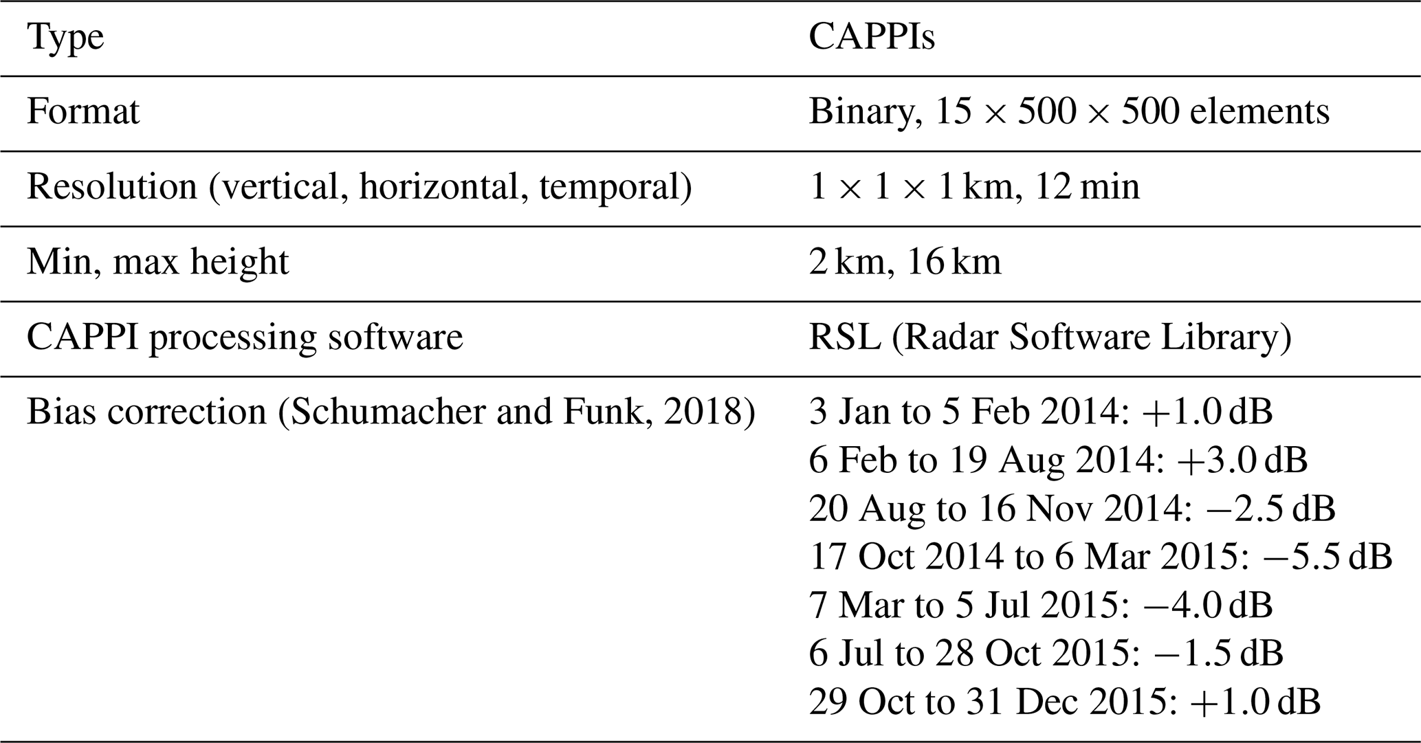

Table 1 SIPAM radar data settings processed by CPTEC-INPE.

Given the coarse characteristics of this radar and its scan strategy, such as varying numbers of elevation sweeps and antenna vibrations between volumes, the radar data used in this study consist of quality-controlled, bias-corrected CAPPIs, gridded onto a 1×1 km horizontal resolution, following previous studies using the same source of data (e.g., Gupta et al., 2024). Following the approach of Saraiva et al. (2016), we restricted our analysis to a 150×150 km box centered on the radar location. This domain allows for consistent and reliable detection of convective structures while also minimizing the effects of beam broadening, ground clutter, and incomplete vertical sampling at farther ranges.

A second data source was employed to calculate parameters related to lightning activity in the convective systems. The Vaisala Global Lightning Detection Network (GLD360; Demetriades et al., 2010) measures cloud-to-ground return strokes in the VLF (very low frequency) range using triangulation techniques, magnetic direction finding (MDF), and time of arrival (TOA), as well as lightning recognition algorithms. Limitations of this network include the detection efficiency in Brazil, which is 70 % in average (Naccarato et al., 2010) but can be significantly lower in areas with deficient coverage such as northern Brazil, including the Amazon region, as well as the definition of a measured stroke as a single or multiple real return strokes (Murphy and Nag, 2015). Stroke data were accumulated over 12 min using the same time stamps as the radar data and were selected within the cluster polygons delimited by the tracking algorithm.

2.2 Tracking methodology

The convective system database was created with the TATHU (Tracking and Analysis of Thunderstorms) software package (Uba et al., 2022) applied to the radar data described in the previous section. The software is a free, open-source Python package available at Uba (2025a), and it addresses convective system tracking as a multi-target tracking problem (Makris and Prieur, 2014). The main modules are observation, detection, description, tracking, and forecast (not used in this study). The algorithm detects agglomerates of pixels – hereafter referred to as clusters of storm cells – in an input field at a single time step according to the (one or more) threshold(s) and extracts their statistics, such as size (in pixels) and mean and maximum values of the input field. From subsequent time steps, based on spatial overlap, it tracks and names (via a universal unique identifier – uuid) the convective systems that occurred in the period and their status during the described life cycle, with status being “spontaneous generation” (new cluster), “continuity” (growing or decaying cluster), “split” (when a single cluster separates into two or more clusters after a time step), or “merge” (when two or more clusters merge into a single cluster after a time step). The identification of a split or a merge depends mainly on the cluster's propagation between subsequent time steps, where discrepancies can occur in situations such as clusters generating within the same relative overlap area of other propagating clusters. This split/merge problem is common to several tracking algorithms that use area overlap strategies, such as SCIT (Storm Cell Identification and Tracking Algorithm; Johnson et al., 1998) and TITAN (Thunderstorm Identification, Tracking, Analysis, and Nowcasting; Dixon and Wiener, 1993).

Table 2 TATHU parameters (original names in parentheses) and values chosen for the generation of the systems (raw) and systems_filtered (filtered) datasets.

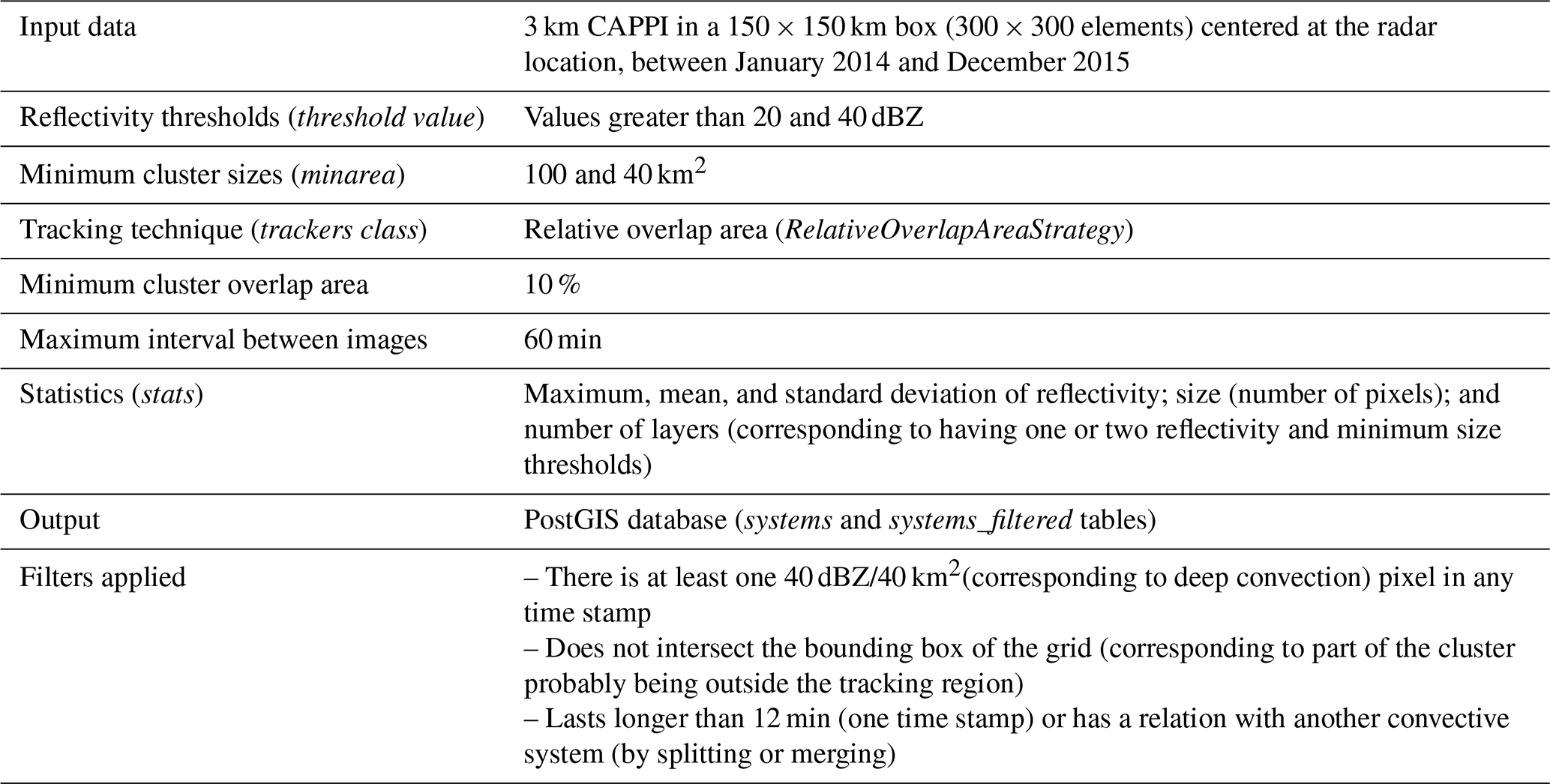
Table 2 shows the TATHU settings used in this study. Based on several considerations, we selected SIPAM radar reflectivity greater than 20 dBZ at the 3 km CAPPI field as the input field to the TATHU tracking algorithm. First, this altitude lies above the typical cloud base in the region (Fisch et al., 2004; Souza et al., 2023) and coincides with the level at which maximum reflectivity is frequently observed in convective precipitation cores below freezing layer. Second, lower elevations near the radar are significantly affected by ground clutter and beam blockage (Giangrande et al., 2016; Schumacher and Funk, 2018), compromising the reliability of reflectivity data closer to the surface. Additionally, the SIPAM radar's relatively coarse resolution limits the ability to resolve vertical structures accurately, particularly storm tilts. However, in the tropical environment of the Amazon, vertical wind shear is generally weak, reducing the likelihood of significant storm tilt or vertical displacement of convective cores. These factors together support the use of a horizontal 3 km CAPPI as a consistent and suitable input for identifying and tracking convective systems in this study. Other tracking algorithms consider composite reflectivity (e.g., Heikenfeld et al., 2019; Sokolowsky et al., 2024) instead of 2D reflectivity fields to offer a more comprehensive depiction of the 3D structure of convective systems. However, considering the context of our study and the nature of this dataset (exposed above), the 3D structure of the convective systems should be captured. A comprehensive study of the implications with respect to the reflectivity thresholds for tracking convective systems in CAPPI fields can be found in Leal et al. (2022) but is not within the scope of this study. Moreover, our approach is methodologically consistent with previous studies that have successfully employed single-level CAPPI fields to characterize convective systems in the Amazon (e.g., Laurent and Laurent, 2002; Albrecht et al., 2011; Leal et al., 2022; Gupta et al., 2024). These studies have provided valuable insights into storm morphology, evolution, and vertical structure using similar techniques. Adopting a comparable methodology ensures continuity and comparability with the existing body of literature on Amazonian convection.

The relative overlap area strategy considers two subsequent clusters in time as the same convective system when there is at least a 10 % overlap between their areas (i.e., polygons). The maximum interval between images considers a data gap sufficient to ensure the continuity of the convective systems, but it can result in different convective systems being tracked as the same system if they are in the overlap area, considering that the average life cycle of tropical convection is less than 60 min. Within the main statistics, clusters with a number of threshold layers equal to 0 (with only the 20 dBZ reflectivity threshold) or 1 (with both the 20 and 40 dBZ reflectivity thresholds) can be used to separate systems with or without deep convective cores.

For better illustration of the terminology of the TATHU tracking system applied to SIPAM 3 km CAPPI fields, Fig. 2 shows a schematic of these definitions: a cluster is a contiguous region (polygon) of pixels within the 3 km CAPPI reflectivity field that exceeds the 20 dBZ reflectivity threshold identified at a single time step; a convective system is a time-continuous sequence of clusters that are linked across radar volumes based on spatial overlap. A cluster can have one or several cores that exceed the 40 dBZ reflectivity threshold, an estimation of deep convection, but these cores are considered to be part of a single cluster during the description and tracking of the convective systems.

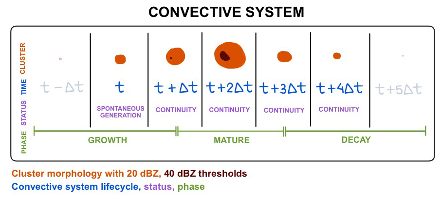
Figure 2 Illustrative deep convective system as observed by TATHU: cluster morphology with 20 dBZ (orange) and 40 dBZ (dark red) thresholds in five valid subsequent time stamps with the TATHU status (spontaneous generation or continuity) and different phases (growth, mature, and decay) of a full life cycle.

Output data were stored in a PostGIS database, a database management system (DBMS) with geospatial support that allows for the storage of large volumes of data in a tabular format, including geolocated geometries. The database was converted to GeoJSON datasets in order to make it easily available in Lopes (2024).

Two datasets were defined based on the TATHU tracking. The original – hereafter referred to as the raw dataset – contains all of the convective systems observed in the period, regardless of duration, size, or status during the life cycle. In contrast, the filtered dataset contains only the convective systems that met the filtering criteria described in Table 2. The second threshold criteria (40 dBZ in a 40 km² minimum area) is used here as a definition of deep convective cores present during the life cycle. Clusters intersecting the borders of the grid had their associated convective systems discarded to exclude systems without a full life cycle within the study area. Systems with only one time step were also discarded. We created this filtered dataset to provide a subset of deep convective systems with a full life cycle, an important criteria for several convection studies.

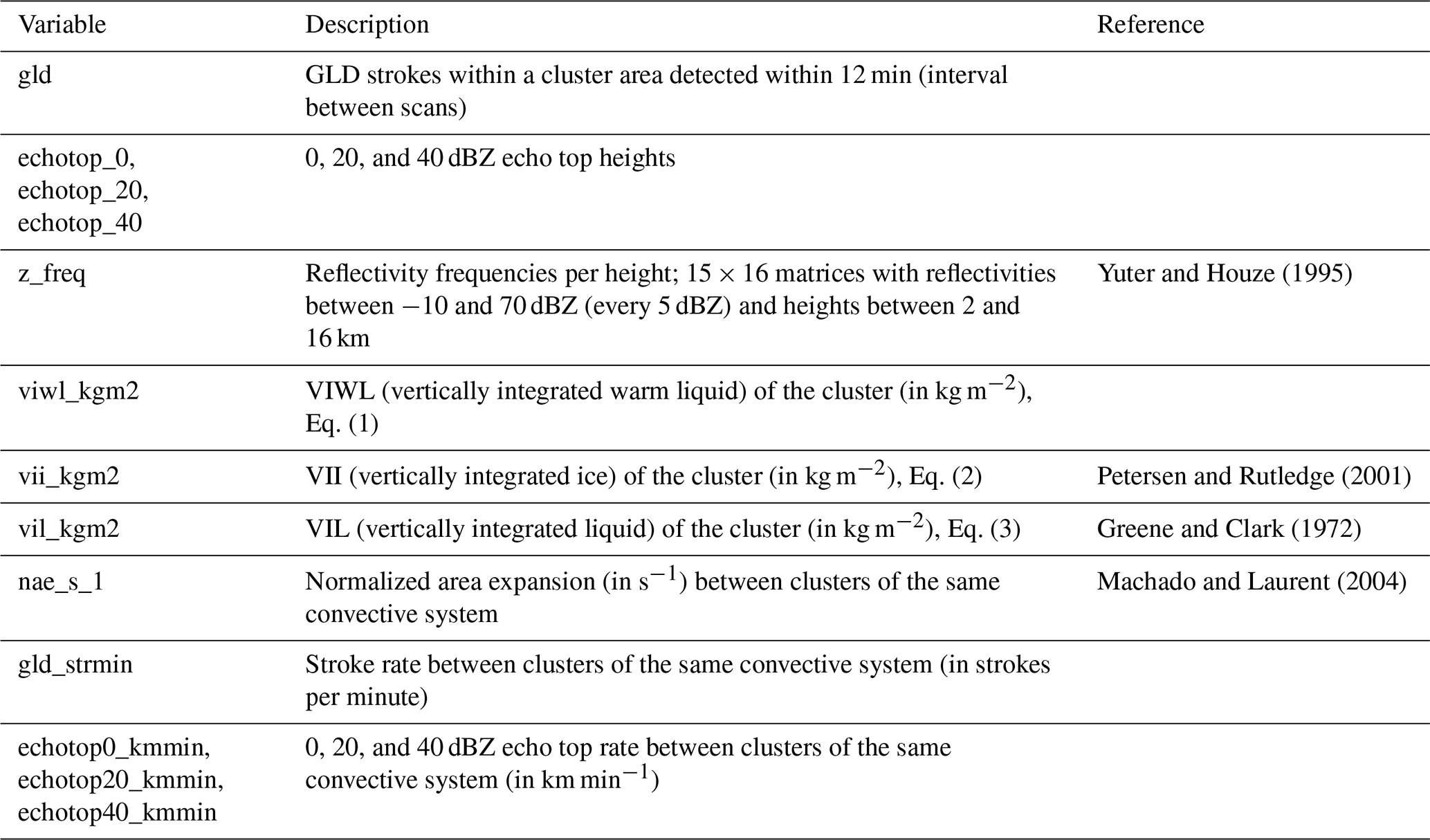
The original systems dataset contains 91 609 convective systems and 322 896 clusters, while the filtered systems_filtered dataset contains 5976 convective systems (6.5 % of the original dataset) and 40 394 clusters (12.5 % of the original dataset). Using the filtered dataset with the additional lightning data, several other parameters were calculated for each cluster (Table 3) related to storm morphology. The following equations were applied for VIWL (vertically integrated warm liquid), VII (vertically integrated ice), and VIL (vertically integrated liquid), respectively:

$$\begin{array}{}\text{(1)}& {\displaystyle }& {\displaystyle }\mathrm{VIWL}=\sum _{i=\mathrm{2}\mathrm{km}}^{\mathrm{5}\mathrm{km}}\mathrm{3.44}\times {\mathrm{10}}^{-\mathrm{6}}{\left({\displaystyle \frac{Z_i+Z_{i+\mathrm{1}}}{\mathrm{2}}}\right)}^{\frac{\mathrm{4}}{\mathrm{7}}},\text{(2)}& {\displaystyle }& {\displaystyle }\mathrm{VII}=\sum _{i=\mathrm{7}\mathrm{km}}^{\mathrm{16}\mathrm{km}}\mathit{\pi }{\mathit{\rho }}_i{N}_o^{\frac{\mathrm{3}}{\mathrm{7}}}{\left[{\displaystyle \frac{\mathrm{5.28}\times {\mathrm{10}}^{-\mathrm{18}}}{\mathrm{720}}}\left({\displaystyle \frac{Z_i+Z_{i+\mathrm{1}}}{\mathrm{2}}}\right)\right]}^{\frac{\mathrm{4}}{\mathrm{7}}},\text{(3)}& {\displaystyle }& {\displaystyle }\mathrm{VIL}=\sum _{i=\mathrm{2}\mathrm{km}}^{\mathrm{16}\mathrm{km}}\mathrm{3.44}\times {\mathrm{10}}^{-\mathrm{6}}{\left({\displaystyle \frac{Z_i+Z_{i+\mathrm{1}}}{\mathrm{2}}}\right)}^{\frac{\mathrm{4}}{\mathrm{7}}}.\end{array}$$

Yuter and Houze (1995)Petersen and Rutledge (2001)Greene and Clark (1972)Machado and Laurent (2004)

Table 3 Clusters' additional parameters calculated on the filtered dataset.

3 Results

3.1 Raw and filtered dataset characteristics

This subsection compares the physical characteristics between the raw and filtered datasets in order to define what type of convective system each dataset represents. Figure 3 shows the size – represented by area (in km²) – distribution of clusters and the maximum size of convective systems. Both distributions have a maximum frequency in the smallest (1000 km²) area. The maximum area of the raw systems is 6 times larger (60 000 km² vs. 10 000 km²) and the distribution drops faster in the filtered systems. These characteristics show the filtering effect around the border of the 150 km bounding box (Fig. 1), which excluded very large clusters. A 200×200 point cluster with a 40 000 km² area, for example, can be considered too large because it occupies two-thirds of the grid and probably intercepts the border of the bounding box in a given time stamp.

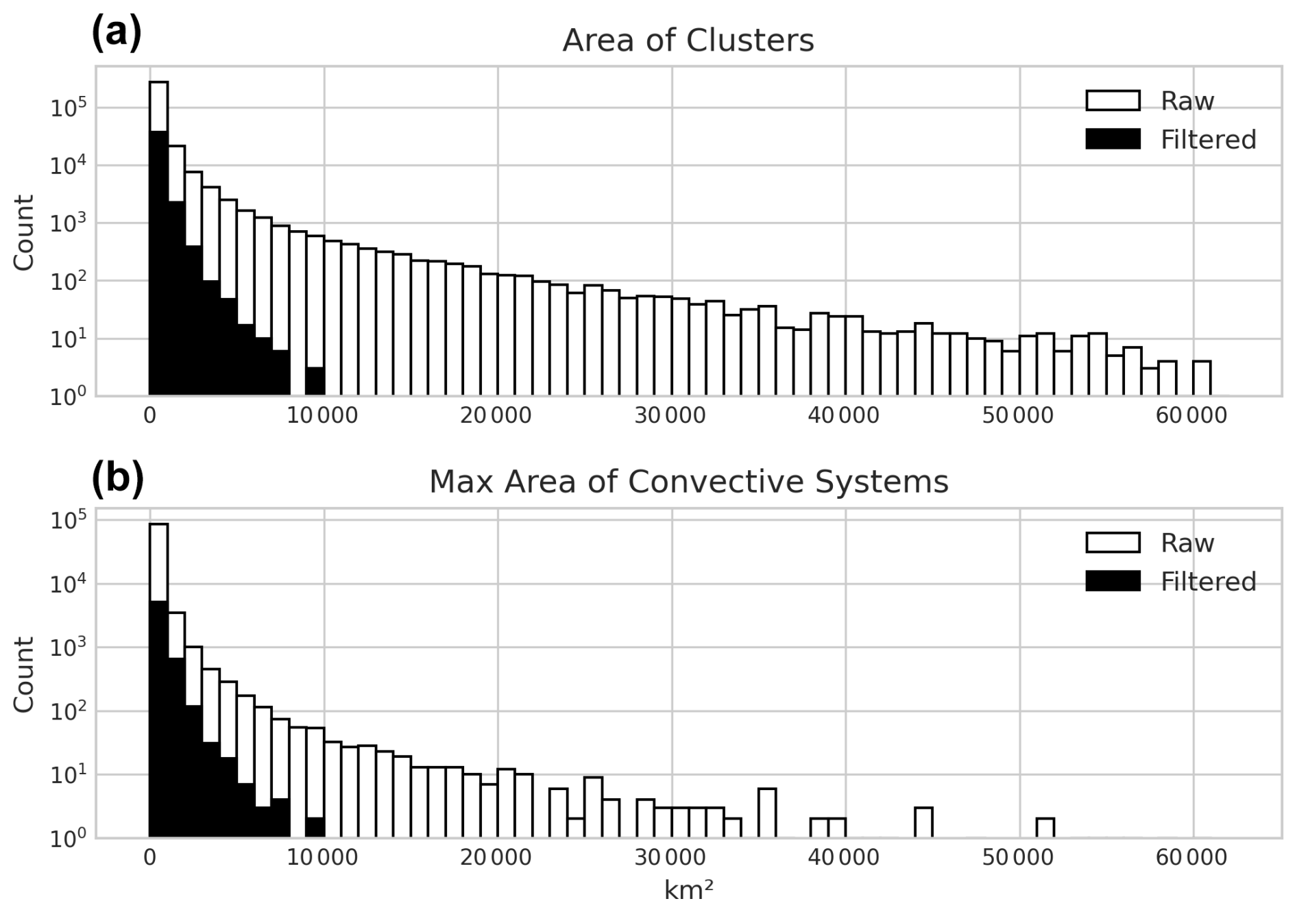
Figure 3 Distribution of clusters' area (a) and convective systems' max area (b) for the raw (white) and filtered (black) datasets.

Figure 4 shows the mean and maximum cluster reflectivity distributions for the raw (Fig. 4a) and filtered (Fig. 4b) datasets. On raw data, the distributions show no significant frequency peaks, with the mean reflectivity distributed mainly (frequency above 20 %) between 20 and 40 dBZ and the maximum reflectivity between 35 and 50 dBZ (frequency above 15 %). Conversely, on the filtered data, peaks (above 35 %) can be found between 25 and 40 dBZ and between 50 and 55 dBZ of mean and maximum reflectivity, respectively. These differences between the distributions represent the filtering effect on the type of the selected clusters. The filters ended up selecting more intense clusters (larger mean and maximum reflectivity) and excluded mainly those that did not exceed 40 dBZ – observe that the clusters with maximum reflectivity below 40 dBZ are significantly less frequent (below 5 %) compared to the raw data ones.

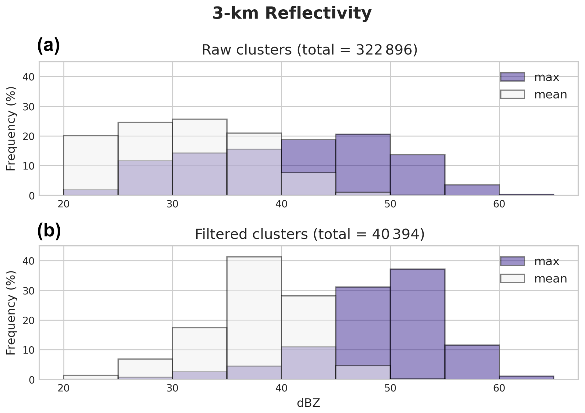
Figure 4 Distribution of clusters' max (purple) and mean (white) reflectivity for raw (a) and filtered (b) datasets.

Table 4 shows some characteristics of the convective systems of the raw and filtered datasets using the cluster classifications on each time step. On both datasets, the percentage of spontaneously generated convective systems was similar (above 70 %); on the raw data, not all of these systems had their full life cycle covered, whereas on the filtered data, all of the systems had their full life cycle covered (as one of the filtering criteria is to exclude convective systems that leave the radar coverage area). A total of 53 % of the filtered convective systems split or merged during their life cycle, compared to 37 % of the raw systems; an important point here is that 31 % of the raw systems and only 2 % of the filtered systems lasted only one time step (12 min) (not shown), meaning that raw convective systems did not last long enough to go through a split or merge. The majority (80 %) of the filtered and half (49 %) of the raw convective systems were considered with their full life cycle (last time step was “continuity”), which is also explained by the high percentage of raw systems with only one time step (i.e., only “spontaneous generation” status). The 20 % of filtered convective systems without a full life cycle are within the not spontaneously generated systems – products of a split or a merge with other systems.

Table 4 Frequency of spontaneously generated (did not generate from splits or the first steps of algorithm rounds) convective systems (CSs), split and/or merged CSs, and full-life-cycle (last time step in continuity) CSs for the raw and filtered datasets.

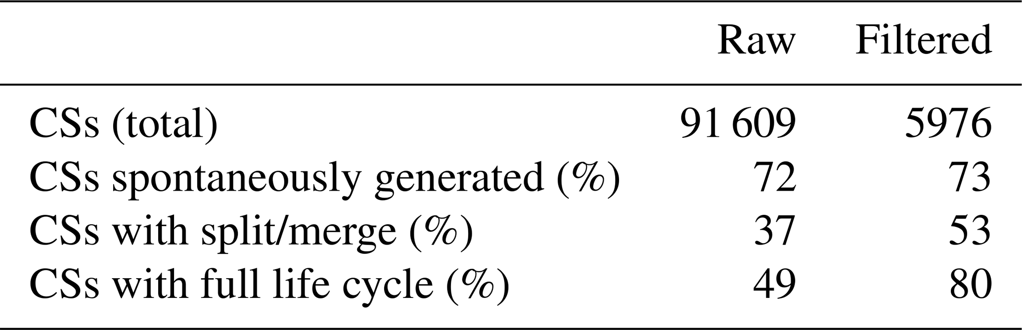
Table 5 shows the distribution of convective system durations for the raw and filtered datasets. The majority of the raw (40 %) and filtered (47 %) systems lasted up to 1 h, indicating the predominance of isolated convective systems (Giangrande et al., 2023; Viscardi et al., 2024; Gupta et al., 2024). Only 10 % of the raw systems lasted between 1 and 3 h, compared to 36 % of filtered systems. The majority of convective systems were short-lived, with 40 % of the raw and 47 % of the filtered systems lasting up to 1 h, highlighting the prevalence of isolated convective systems. A notable difference is observed in the 1–3 h range, where only 10 % of the raw systems persisted, compared to 36 % in the filtered dataset. For long-duration systems, nearly twice as many raw systems (631) lasted longer than 6 h compared to those in the 5–6 h range (318). In contrast, the filtered dataset shows fewer systems exceeding 6 h (18) than those lasting between 5 and 6 h (27), indicating a stronger effect of the area filtering on prolonged convective systems.

Table 5 Frequency of spontaneously generated (did not generate from splits or the first steps of algorithm rounds) CSs, split and/or merged CSs, and full-life-cycle (last time step in continuity) CSs for the raw and filtered data tables.

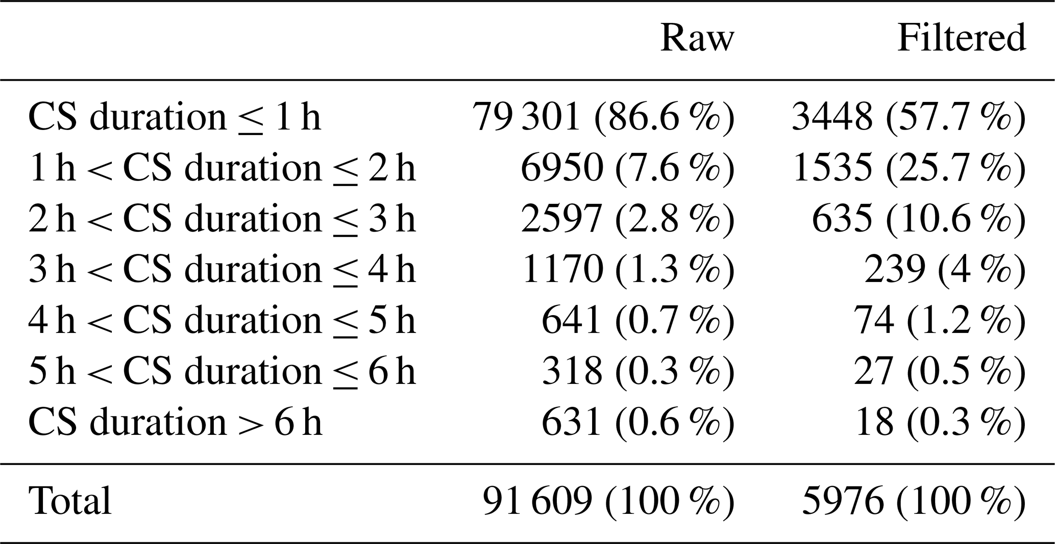
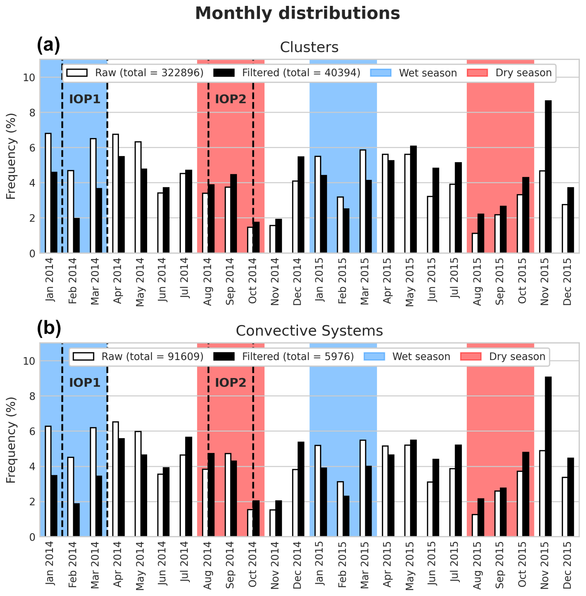
Figure 5 Monthly relative frequency distribution of clusters (a) and convective systems (b) for the raw (white) and filtered (black) datasets. The blue and red areas delimit wet and dry seasons, respectively, and dashed lines delimit IOP1 and IOP2.

Table 6 Distribution of convective system (CS) durations for the raw and filtered datasets separated by IOP1 and IOP2.

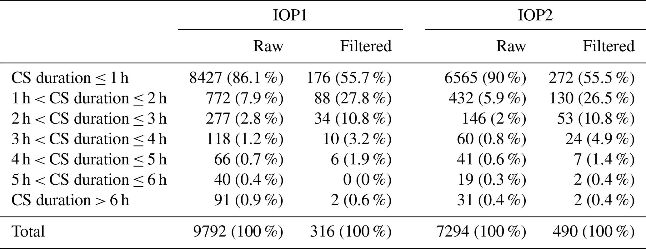
Figure 5 shows the monthly distribution of the raw and filtered clusters and convective systems. Seasons and intensive operation periods (IOPs) were defined according to Machado et al. (2018): dry season between August and October, dry-season–wet-season transition between November and December, wet season between January and March, IOP1 between February 1 and March 31 2014, and IOP2 between 5 August and 15 October 2014. In general, a larger frequency of clusters and convective systems occurred in the wet and transition (wet-to-dry and dry-to-wet) seasons, with a peak in the filtered clusters/systems in November 2015 (almost 2 times more than the raw clusters/systems). The proportion between raw and filtered systems changes over the months, with a larger frequency of raw clusters and convective systems in the wet seasons and the opposite in the dry seasons. This difference can be explained by the filtering of very large clusters cited previously, which are more common in the wet season. Considering the climatological characteristics of each season, it is expected that more clusters/convective systems would occur during the wet season than during the dry season, which was the case for both the raw and filtered data.

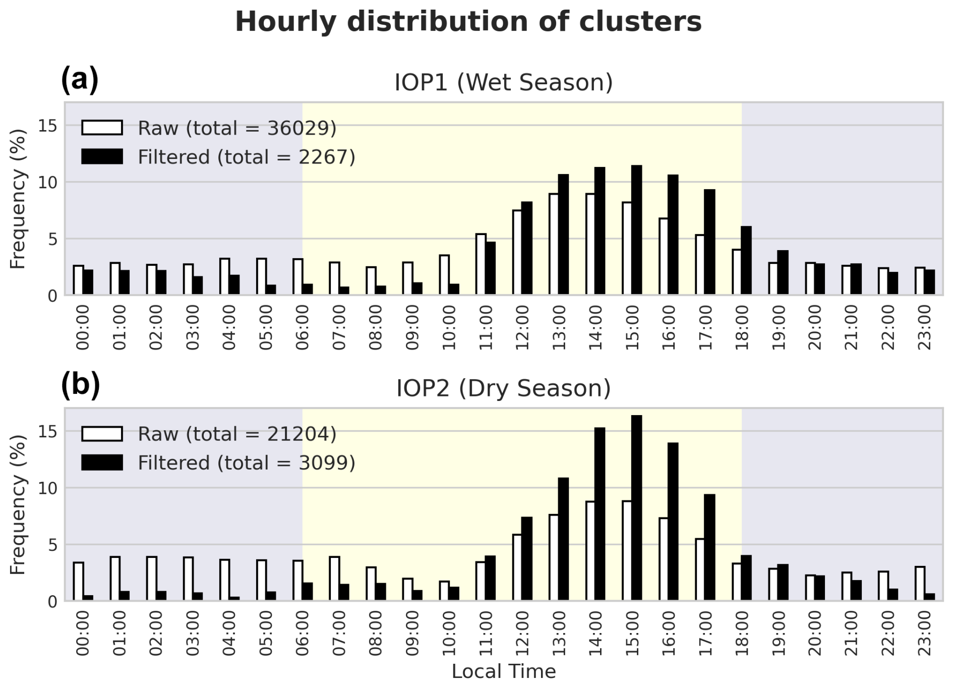
Figure 6 Hourly relative distribution of clusters for the raw (white) and filtered (black) datasets separated by IOP1 (a) and IOP2 (b). The blue and yellow areas delimit diurnal and nocturnal periods, respectively.

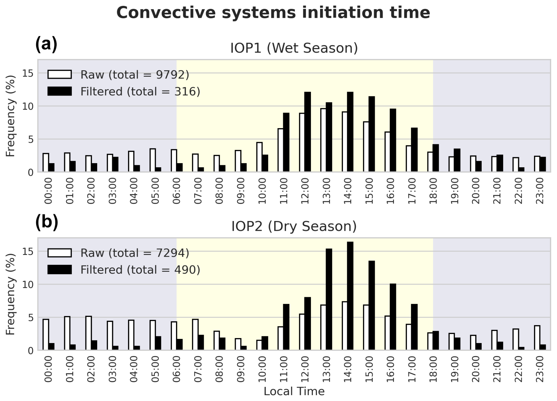
Figure 7 Hourly relative distribution of convective system initiation time for the raw (white) and filtered (black) datasets separated by IOP1 (a) and IOP2 (b). The blue and yellow areas delimit diurnal and nocturnal periods, respectively.

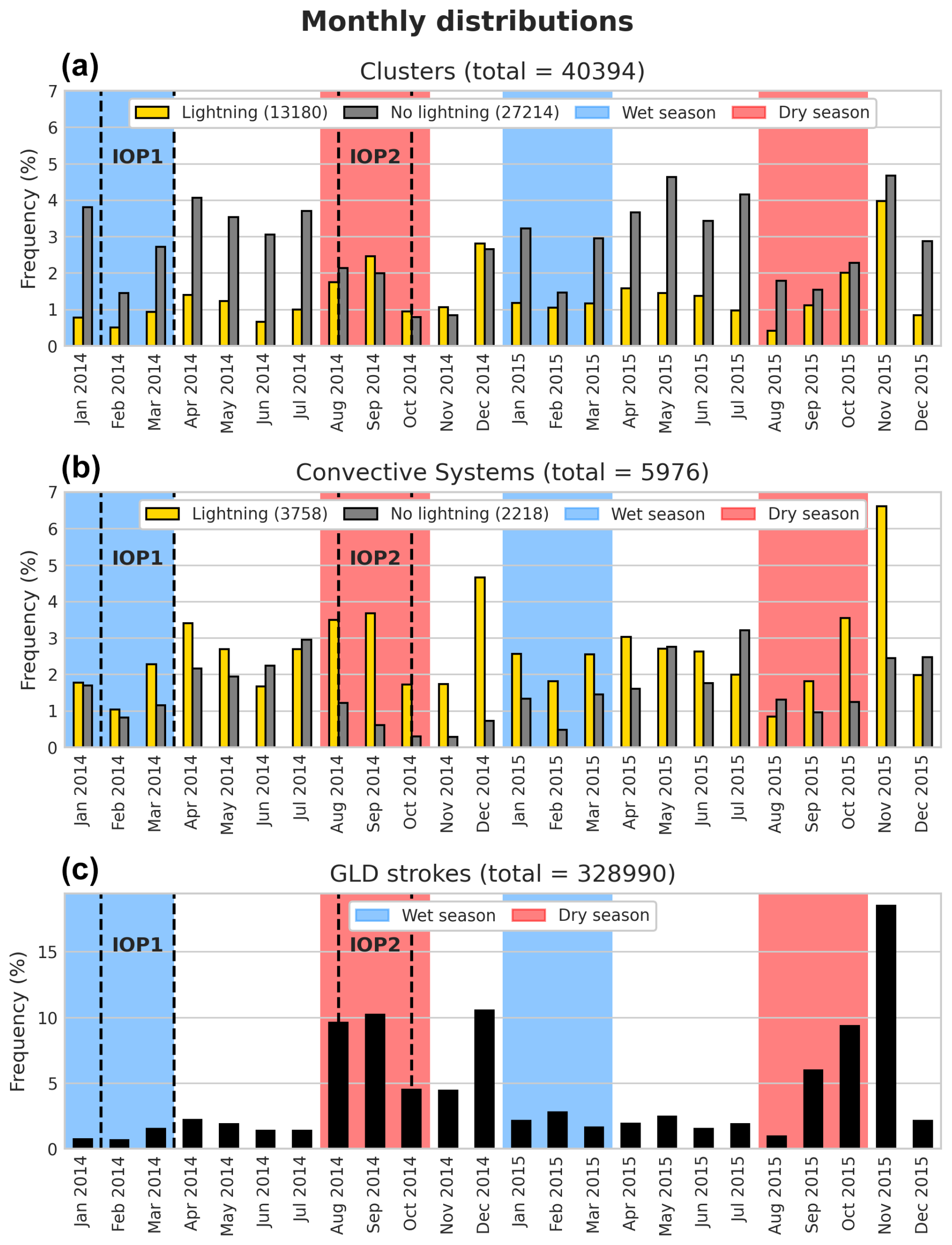
Figure 8 Monthly relative distribution of clusters (a), convective systems (b), and GLD strokes (c) for filtered datasets separated by lightning (yellow bars) or no lightning (gray bars) occurrence. The blue and red areas delimit wet and dry seasons, respectively, and dashed lines delimit IOP1 and IOP2.

Table 6 presents the duration of the raw and filtered convective systems by IOP. The distribution of system durations is generally consistent across seasons, with similar proportions observed between the raw and filtered datasets. In contrast to Table 5, where less than half of the raw systems lasted up to 1 h, seasonal distributions show that more than 80 % of the raw systems and 50 % of filtered systems persisted for no more than 1 h, indicating the predominance of isolated convective systems. Additionally, 97 % of raw and 94 % of filtered systems had durations of 3 h or less.

Figure 6 shows the hourly distribution of the raw and filtered clusters by IOP. Comparing the raw and filtered clusters, in all seasons, there is a larger frequency of raw clusters during the late-night/dawn period and a larger frequency of filtered clusters during late-morning/afternoon period. In the dry season (IOP2), filtered clusters are more frequent (above 15 %) between 14:00 and 15:00 LT (local time) compared to the raw clusters (below 10 %), while the raw clusters are 5 % more frequent than the filtered clusters between 23:00 and 07:00 LT. These differences between the raw and filtered clusters indicate a more diurnal characteristic of the filtered clusters, while the raw clusters are more nocturnal, probably represented by the very large and long-lasting (above 6 h) clusters described previously.

Figure 7 shows the hourly distribution of the raw and filtered convective system initiation (defined here as the first time stamp) by IOP. Comparing the raw and filtered systems, in both seasons, there is a larger frequency of raw systems initiating at dawn, whereas a larger frequency of filtered systems initiate during the morning/afternoon. This difference is even greater (almost 10 %) in the dry season. Comparing the seasons, in both the dry and wet seasons, the initiation peak occurs only at 14:00 LT. Specifically regarding the filtered systems, the 14:00 LT peak during the wet season is not highlighted in IOP1, with another peak at 12:00 LT.

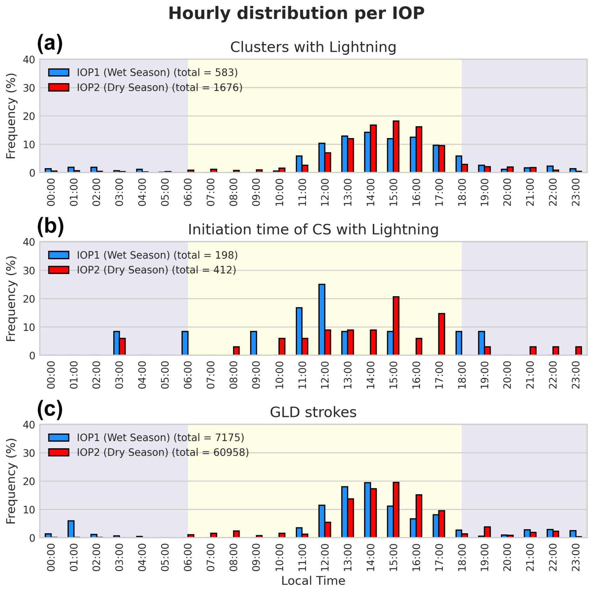
Figure 9 Hourly relative distribution of clusters with lightning (a), initiation time of clusters with lightning (b), and GLD strokes (c) for filtered dataset during IOP1 (blue) and IOP2 (red). The blue and yellow areas delimit diurnal and nocturnal periods, respectively.

When comparing the physical characteristics of the raw and filtered datasets, the filters significantly decrease the sampling size but define a specific subset of convective systems: in general, they have areas of up to 10 000 km², a maximum reflectivity mainly above 50 dBZ, a full life cycle (growth, mature, and decay phases), and last up to 3 h. The raw dataset includes these same systems as well as diverse convective types, such as mesoscale (considering the areas above 50 000 km²), both short-lived (12 min duration) and long-lived (duration above 6 h), and stratiform (reflectivity below 30 dBZ) systems. Both datasets are useful for further convection studies, but they should be chosen carefully depending on the study objectives. If the convection phase is important, for example, the filtered dataset would be more appropriate, whereas some studies might benefit from convection patterns in the Amazon region that can be extracted from the raw dataset.

3.2 Characteristics specific to the filtered systems

Starting with the monthly distribution, Fig. 8 shows the clusters and convective systems separated by lightning activity as well as the distribution of GLD strokes. More than double the clusters (27 214 vs. 13 180) had no electrical activity, while more convective systems (3758 vs. 2218) showed lightning, which means that, in general, the convective systems with lightning consist of only a few clusters with lightning. A larger frequency of clusters and systems without lightning occurs between wet and dry seasons, while peaks in cluster and system frequency occur in the dry-season–wet-season transition, comparable with the peak stroke frequency. These findings are similar to what has been found in previous work such as Albrecht et al. (2011, 2016).

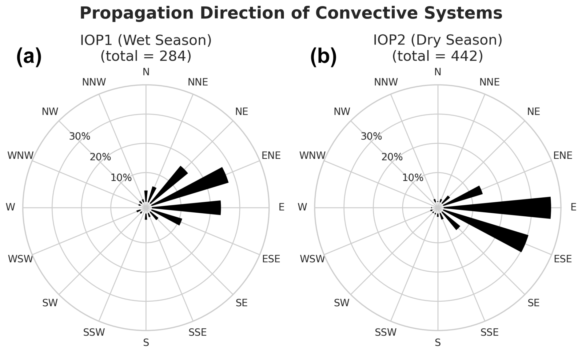
Figure 10 Convective systems' relative propagation direction distribution in the filtered dataset separated by IOP1 (a) and IOP2 (b). The direction was defined by the distance between the first and last centroids of the convective system.

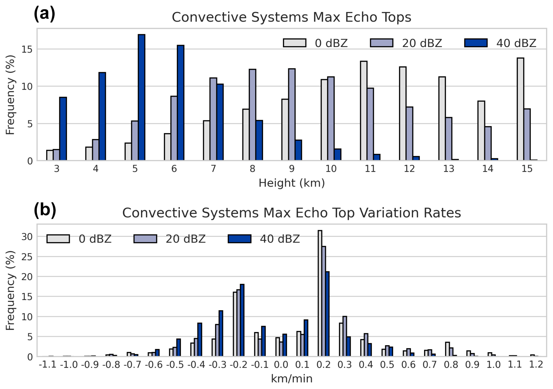
Figure 11 Convective systems' 0 (gray bars), 20 (light-blue bars), and 40 dBZ (dark-blue bars) max echo tops (a) and max echo top variation rates (b).

Separating the analysis into systems with and without lightning, Fig. 9 shows the hourly distribution of clusters and the initiation (first time stamp) of convective systems with lightning and GLD strokes by IOP. All variables are more frequent during the late-morning/afternoon period, with significant differences between IOPs. In IOP2, the cluster and stroke peaks occur at 15:00 LT, which is also the preferential time for convective system initiation. In IOP1, the cluster and stroke peaks occur around the same time, but system initiation occurs preferentially earlier, at 12:00 LT. The low number of systems (198 in IOP1 and 412 in IOP2) influenced the frequency distribution, but the results were similar to their corresponding seasons (not shown). Convective systems without lightning are more frequent during the late-morning/afternoon period (not shown). The initiation frequency peaks in the dry and wet seasons occur at 15:00 LT, whereas during the dry-season–wet-season transition, the distribution is more dispersed, with approximately equal peaks at 12:00, 13:00, and 16:00 LT.

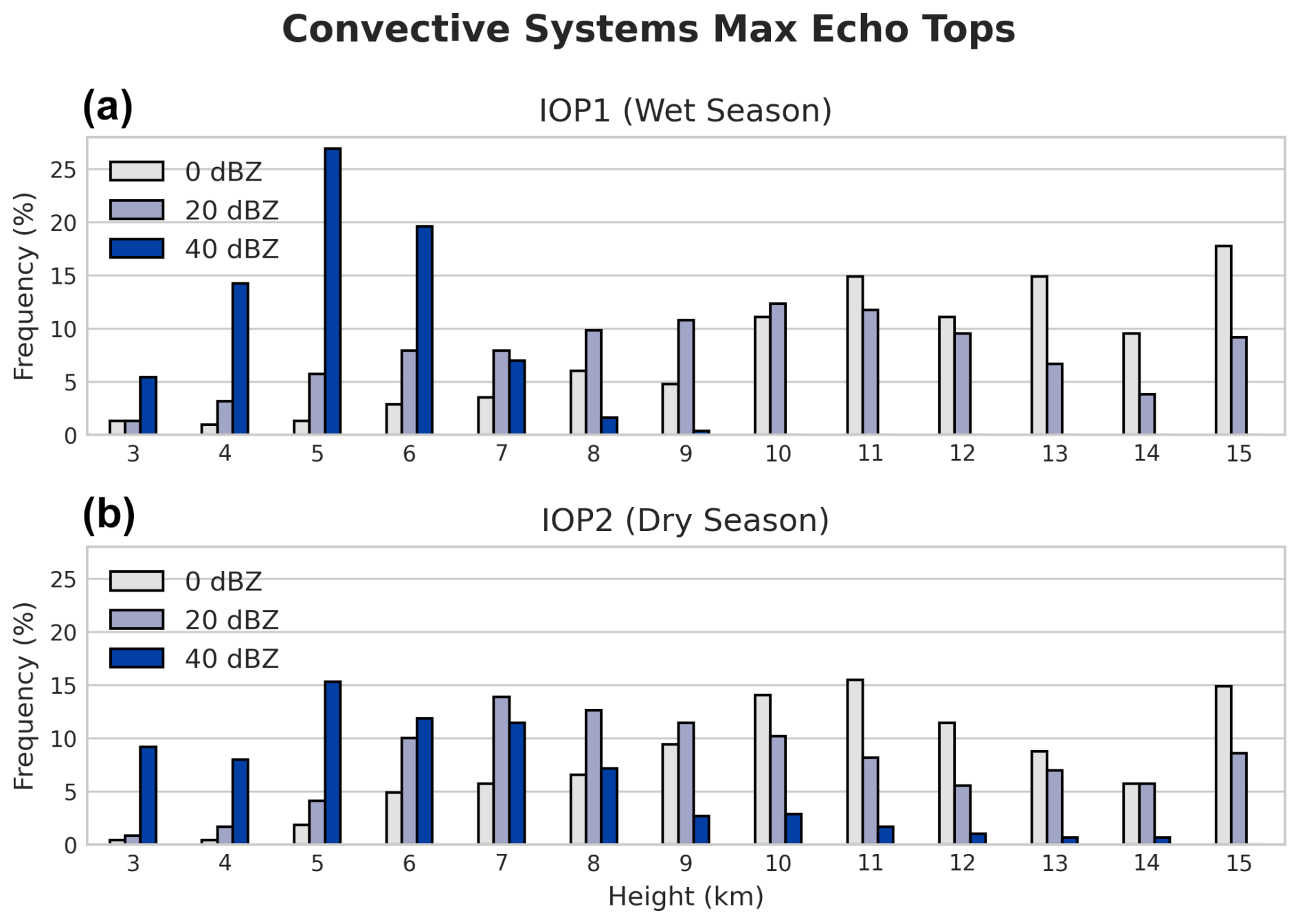
Figure 12 Convective systems' 0 (gray bars), 20 (light-blue bars), and 40 dBZ (dark-blue bars) max echo tops separated by IOP1 (a) and IOP2 (b).

In order to analyze the propagation direction of the convective systems, Fig. 10 shows the frequency distribution of the propagation direction by IOP. The predominant direction of the convective systems is from the east, consistent with the main dynamic forcing in the Amazon, which is a moisture flux from the tropical Atlantic due to the easterlies that is influenced by the position of the Intertropical Convergence Zone (ITCZ) (Silva Dias and Carvalho, 2016). Comparing the IOPs, in the wet season, about 25 % of systems propagated from the east and east-northeast, whereas in the dry season, more than 30 % of systems propagated from the east and east-southeast. This direction shift from east-northeast to east-southeast is related to the shift in the position of the ITCZ and cold-front propagation over the South American continent, which affect the zonal wind regime in the Amazonian region (Rickenbach et al., 2002). These results are also consistent with Gupta et al. (2024), who focused on isolated convective systems near the Manacapuru (T3) site.

In order to analyze the intensity of the convective systems, Fig. 11 shows the frequency distribution of the maximum heights and variation rates (considering the 12 min interval between radar scans) of the 0, 20, and 40 dBZ echoes, associated with cloud-top height, precipitable-hydrometeor height, and intense-precipitation height, respectively. The maximum cloud-top heights are more frequent above 10 km, with peaks at 11 km (dry season) and 15 km (wet season). The maximum precipitable-hydrometeor height was more frequent between 7 and 11 km. The maximum intense-precipitation height was also more frequent between 4 and 7 km, with peaks at 5 km (in both the dry and wet seasons). These high tops, complemented by a maximum precipitation height more frequently between 7 and 11 km and a maximum intense-precipitation height more frequently between 4 and 7 km, show how these systems were predominantly deep at their most intense moments. The variation rates (Fig. 11b) were similar between the echoes, with frequency peaks at −0.2 and 0.2 km min⁻¹, indicating significant fluctuations in the echo tops throughout their life cycle.

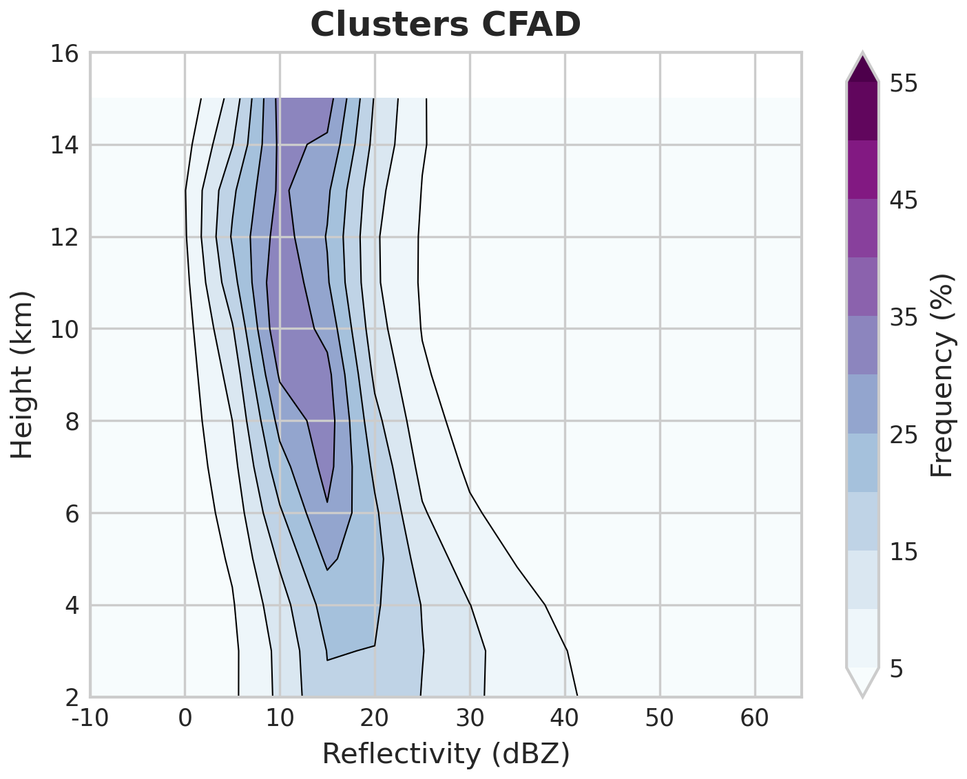
Figure 13 Mean contoured frequency by altitude diagram (CFAD) of clusters' reflectivity with 5 dBZ bins.

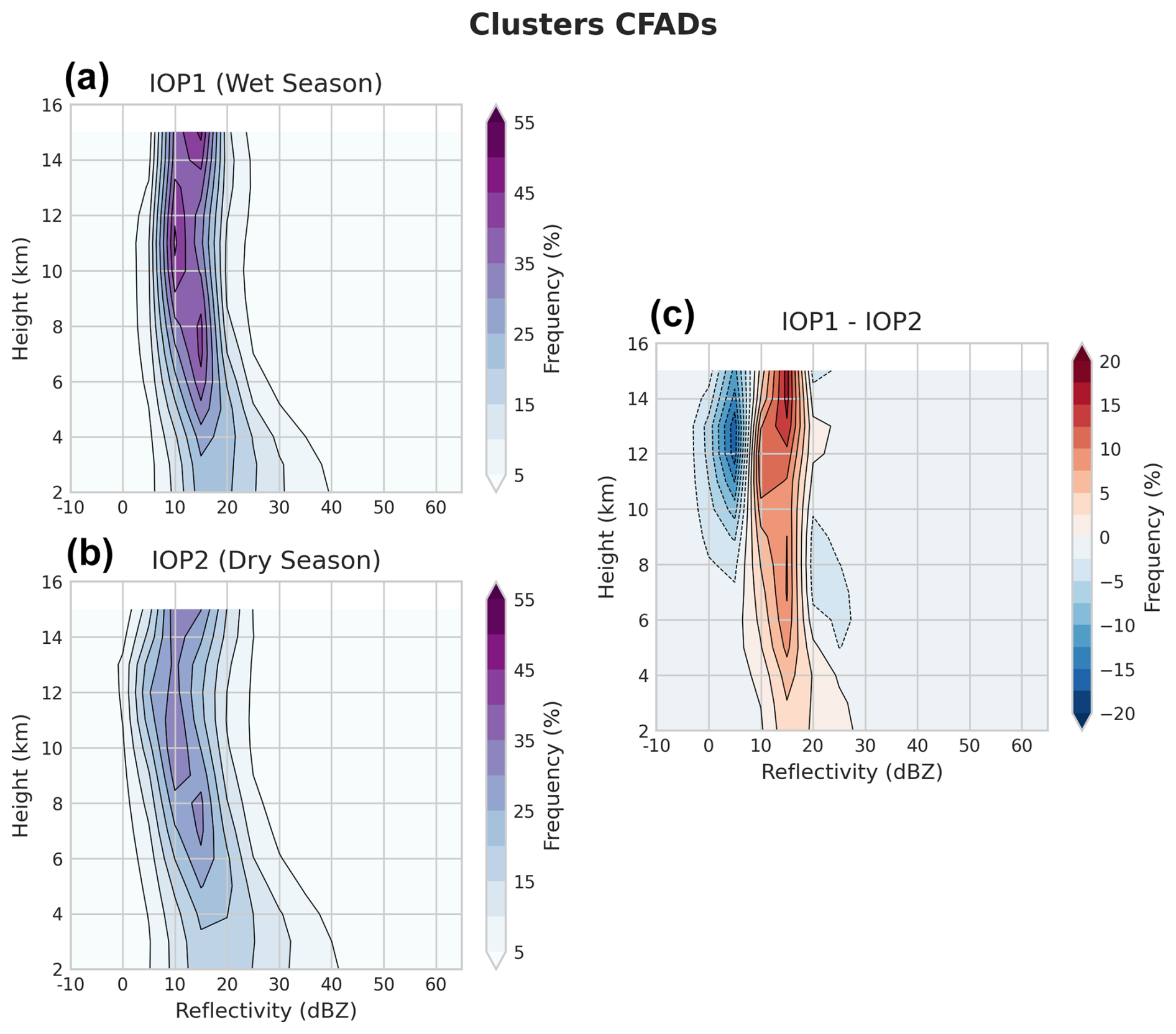
Figure 14 Mean contoured frequency by altitude diagram (CFAD) of clusters' reflectivity with 5 dBZ bins separated by IOP1 (a) and IOP2 (b); the IOP1 − IOP2 anomaly (c) is also shown.

Figure 12 shows the frequency distribution of the maximum echo tops of 0, 20, and 40 dBZ by IOP. As in the complete time series, the maximum top heights are more frequent above 10 km, with peaks at 11 km (IOP2) and 15 km (IOP1). The maximum precipitable height was also more frequent between 7 and 11 km. The maximum intense precipitation height was also more frequently located between 4 and 7 km, with peaks at 5 km.

In order to analyze the clusters' vertical profiles, Fig. 13 shows the frequency diagram by altitude of the cluster reflectivity of the complete time series. The most frequent profile is of a small reflectivity variation with height: 25 dBZ at the surface to 10 dBZ at 15 km height (i.e., a −1 dBZ km⁻¹ variation). Less frequent (between 5 % and 10 %) profiles have very low (5 to 10 dBZ) or high (40 dBZ) reflectivity at the surface and up to 25 dBZ at 15 km height, with a minimum of 0 dBZ at 12 km height.

Figure 14 shows the clusters' frequency by altitude diagrams by IOP as well the difference between them. Considering the largest frequencies, the profiles are similar between the IOPs (and with the complete time series profile), but the IOP1 profile (wet season) is more intense (up to 20 %) than IOP2 profile (dry season), especially between 10 and 20 dBZ.

4 Data availability

The systems and systems_filtered datasets are available at https://doi.org/10.5281/zenodo.13732692 (Lopes, 2024). SIPAM radar data are available at https://ftp.cptec.inpe.br/chuva/goamazon/experimental/level_0/eq_radar/esp_band_s/st_sipam/ (Biscaro, 2016).

5 Code availability

The TATHU software package is available at https://doi.org/10.5281/zenodo.17298147 (Uba, 2025a). The code developed to create the datasets with TATHU is available at https://doi.org/10.5281/zenodo.17297271 (Uba, 2025b).

6 Conclusions

A database of convective systems that occurred during the GoAmazon experiment was created to provide a comprehensive convection data collection for future GoAmazon studies. The systems and systems_filtered datasets cover the main convective characteristics (including morphology and intensity) and electrical activity. The filtered dataset is shown to be an acceptable sample of the complete dataset, selecting deep convective systems with a full life cycle within the research area. Convection seasonality is also well represented, with more intense convective systems between the dry season and the dry-season–wet-season transition and less intense systems in the wet season, typically occurring during the late-morning/early-afternoon period. The preeminent propagation direction of these systems is connected with the easterlies, with a transition from slightly north to slightly south associated with the ITCZ position.

It is important to consider the limitations in the convection description when using these data for future research. As the SIPAM radar's main role is to serve as an operational weather radar instrument, its settings are not optimal for convection research: low spatial (1 km) and temporal (12 min) resolution (considering it is a weather radar), beam blockage during the experiment (Giangrande et al., 2016; Tian et al., 2021), and radar software setting changes during the experiment. Another limitation is in the tracking itself, especially when dealing with system splitting/merging (which occurs in a significant portion of the convective system database), which can be more complex in large, mesoscale systems. Even with these limitations, the database is an important source of convection characteristics for cloud–aerosol–precipitation research.