A seamless global daily 5 km soil moisture product from 1982 to 2021 using AVHRR satellite data and an attention-based deep learning model

Soil moisture (SM) data records longer than 30 years are critical for climate change research and various applications. However, only a few such long-term global SM datasets exist, and they often suffer from large biases, low spatial resolution, or spatiotemporal incompleteness. Here, we generated a consistent and seamless global surface SM product (0–5 cm) spanning 1982–2021 using a deep learning (DL) model. The model was trained with the GLASS-MODIS SM product and was designed to integrate four decades of Advanced Very High Resolution Radiometer (AVHRR)-derived albedo and land surface temperature, the land component of the fifth generation of European ReAnalysis (ERA5-Land) SM, and terrain and soil texture datasets as input features. Considering the temporal autocorrelation of SM, we explored two types of DL models that are adept at processing sequential data, including three long short-term memory (LSTM)-based models, i.e., the basic LSTM, bidirectional LSTM (Bi-LSTM), and attention-based LSTM (AtLSTM), and a transformer model. We also compared the performance of the DL models with the tree-based eXtreme Gradient Boosting (XGBoost) model, known for its high efficiency and accuracy. Our results show that all four DL models outperformed the benchmark XGBoost model, with the AtLSTM model achieving the highest accuracy on the test set, particularly at high SM levels ($>\mathrm{0.4}{\mathrm{m}}^{\mathrm{3}}{\mathrm{m}}^{-\mathrm{3}}$). These results suggest that under some challenging conditions, utilizing temporal information and adding an attention module can effectively enhance the estimation accuracy of SM. Subsequent analysis of attention weights revealed that the AtLSTM model could automatically learn the necessary temporal information from adjacent positions in the sequence, which is critical for accurate SM estimation. The best-performing AtLSTM model was then adopted to produce a four-decade seamless global SM dataset at 5 km spatial resolution, denoted as the GLASS-AVHRR SM product. Validation of the GLASS-AVHRR SM product using 45 independent International Soil Moisture Network (ISMN) stations prior to 2000 yielded a median correlation coefficient (R) of 0.73 and an unbiased root mean square error (ubRMSE) of 0.041 m³ m⁻³. When validated against SM datasets from three post-2000 field-scale COsmic-ray Soil Moisture Observing System (COSMOS) networks, the median R values ranged from 0.63 to 0.79, and the median ubRMSE values ranged from 0.044 to 0.065 m³ m⁻³. Further validation across 22 upscaled 9 km Soil Moisture Active Passive (SMAP) core validation sites indicated that it could well capture the temporal variations in measured SM and remained unaffected by the large wet biases present in the input ERA5-Land SM product. Moreover, characterized by complete spatial coverage and low biases, this four-decade, 5 km GLASS-AVHRR SM product exhibited high spatial and temporal consistency with the 1 km GLASS-MODIS SM product and contained much richer spatial details than both the long-term ERA5-Land SM product (0.1°) and European Space Agency Climate Change Initiative combined SM product (0.25°). The annual average GLASS-AVHRR SM dataset from 1982 to 2021 is available at https://doi.org/10.5281/zenodo.14198201 (Zhang et al., 2024b), and the complete product can be freely downloaded from https://glass.hku.hk/archive/SM/AVHRR/ (last access: 18 September 2025).

1 Introduction

Soil moisture (SM) is an essential climate-sensitive variable that exhibits high spatial and temporal variability. It can be measured directly by in situ sensors or indirectly through model simulations or remote sensing techniques (Liang and Wang, 2020). Accurate knowledge of the spatial and temporal distribution of SM can benefit applications across various Earth system domains, including climate, hydrology, and agriculture (Dorigo et al., 2017; Peng et al., 2021a). While local- to regional-scale hydrological and agricultural applications like watershed runoff modeling, evapotranspiration estimation, and crop yield prediction demand SM products with high spatial resolution (≤1 km) (Hssaine et al., 2018; Schoener and Stone, 2019; Zhuo et al., 2019), continental- to global-scale climate-change-related applications, such as SM trend analyses and drought monitoring, generally require long-term data availability (>30 years), in addition to moderate spatial resolution and high accuracy (Cheng et al., 2015; Grillakis, 2019).

Long-term point-scale SM can be measured directly by in situ sensors; thus, great efforts have been devoted worldwide to deploying and maintaining a series of operational SM networks. In situ SM datasets from some networks were shared by data organizations, which were then processed and released in a harmonized format to the public by the International Soil Moisture Network (ISMN) data repository (Dorigo et al., 2021). Still, these networks are too sparse and unevenly distributed in space, and each covers a different observation period, hindering their use in large-scale applications. Currently, large-scale SM products are typically obtained through model simulations or remote sensing techniques. Driven by long-term forcing variables, land surface models or data assimilation systems can simulate decades of spatiotemporally continuous SM products at the global scale, with an increasingly finer spatial resolution. Several commonly used SM products include those generated by the Modern-Era Retrospective analysis for Research and Applications version 2 (MERRA-2) at 0.5° from 1980 to the present (Gelaro et al., 2017), the Global Land Data Assimilation System version 2 (GLDAS-2) at 1°$/$0.25° from 1948 to the present (Rodell et al., 2004), and the land component of the fifth generation of European ReAnalysis (ERA5-Land) at 0.1° from 1950 to the present (Muñoz-Sabater et al., 2021). Recently, models that focus on the dynamic simulation of evapotranspiration and SM, such as the fourth generation of the Global Land Evaporation Amsterdam Model (GLEAM4) (0.1°, 1980–2023) and the Simple Terrestrial Hydrosphere model version 2 (SiTHv2) (0.1°, 1982–2020), have also provided long-term global SM products by integrating multi-source satellite data and hydrometeorological variables (Miralles et al., 2025; Zhang et al., 2024a). Yet, these SM products may suffer from large uncertainties arising from defective forcing data, imperfect model parameterization, and the uneven spatial distribution of input meteorological observations, particularly the limited observational coverage in tropical regions (Ling et al., 2021; Zhang et al., 2024a).

Alternatively, microwave remote sensing techniques have been utilized for SM retrieval since the 1970s (Schmugge et al., 1974). Various global SM products have been developed from a range of active or passive microwave sensors, such as the advanced scatterometer aboard the Meteorological Operational satellites (Bartalis et al., 2007), the microwave radiation imager on Fengyun-3 satellites (Kang et al., 2021), and the L-band radiometers on the Soil Moisture and Ocean Salinity (SMOS) and Soil Moisture Active Passive (SMAP) satellites (Chan et al., 2018; Entekhabi et al., 2010; Kerr et al., 2012; Li et al., 2022c, b; Wigneron et al., 2021). However, the temporal coverage of these single-sensor SM products is typically short, as constrained by the operational lifespan of the satellites. In this context, the European Space Agency (ESA) Climate Change Initiative (CCI) program released a long-term global SM product spanning the period since 1978, which merged multiple active and passive microwave SM products retrieved from different satellite instruments (Dorigo et al., 2017). Despite being the longest satellite SM dataset currently available, the ESA CCI combined SM product has a relatively low spatial resolution (0.25°) and incomplete spatial coverage, which may restrict its usage in certain applications. According to Zheng et al. (2023), the percentage of missing data in the ESA CCI combined SM product ranges from 21.8 % to 94.41 % at the daily scale during the period from 2000 to 2020.

In contrast, optical and thermal remote sensing techniques are characterized by long observation period, rich spectral bands, and high spatial resolution, but their relatively low sensitivity to SM poses challenges in deriving the long-term global SM product solely from optical and thermal satellite observations. Over the past few decades, optical and thermal datasets have been extensively employed to downscale the coarse-scale microwave or model-simulated SM products. Most of these downscaling studies empirically or physically relate vegetation and temperature parameters to SM conditions based on the universal triangle concept (Gillies and Carlson, 1995; Merlin et al., 2012; Piles et al., 2011). For a detailed review of the strengths and limitations of various SM downscaling algorithms, refer to Sabaghy et al. (2018). In recent years, machine learning models have gradually gained popularity in SM estimation and the downscaling of coarse-scale SM products, such as the SMAP, ERA5-Land, and ESA CCI SM products (Cheng et al., 2023; Guevara et al., 2021; Karthikeyan and Mishra, 2021; Zhang et al., 2023; Zheng et al., 2023), due to their flexibility to integrate multi-source datasets and ability to implicitly learn the non-linear relationships between SM and its influencing factors. However, the above-mentioned downscaling studies primarily concentrated on enhancing the spatial resolution of SM products, typically through integrating the fine-scale Moderate Resolution Imaging Spectroradiometer (MODIS) datasets, and there is still a lack of focus on developing long-term SM products or utilizing the four-decade Advanced Very High Resolution Radiometer (AVHRR) observations for long-term SM estimation.

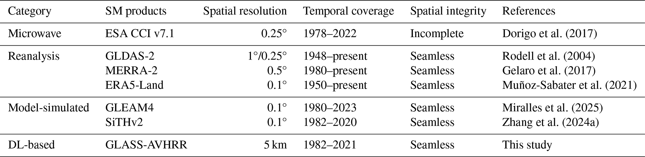
Compared with conventional machine learning models, deep learning (DL) models can automatically extract relevant features from raw datasets and learn complex non-linear relationships between variables, without the need for careful feature engineering (LeCun et al., 2015). Recently, significant progress has been made in applying DL techniques to a range of environmental remote sensing research areas, including land cover mapping (Huang et al., 2018), data fusion and downscaling (Wang et al., 2021), and environmental parameter retrieval (Ma and Liang, 2022; Yuan et al., 2020). In terms of SM retrieval, Fang et al. (2017) first utilized a long short-term memory (LSTM) model to predict spatiotemporally continuous SM over the continental United States, with atmospheric forcings, modeled SM, and static attributes employed as input features and the SMAP SM product serving as the training target. Since then, various DL models have been used in SM estimation (Gao et al., 2022; Sungmin and Orth, 2021), downscaling (Xu et al., 2022; Zhao et al., 2022), forecasting (Fang and Shen, 2020; Li et al., 2022a), and gap-filling (Zhang et al., 2022; Zhou et al., 2023) studies. Among them, the most frequently used DL models were the LSTM-based models designed to capture temporal information from sequential data and the convolutional neural network (CNN)-based models constructed to extract spatial patterns from grid data, alongside several other models such as the deep neural network and deep belief network. In those studies, input features might include brightness temperature, surface reflectance, meteorological forcings, terrain and soil properties, land cover, precipitation, and land surface temperature (LST), depending on the types of models they aimed to simulate, such as radiative transfer models, downscaling models, or land surface models, while the training target varied from point-scale in situ SM to coarse-scale microwave or simulated SM. Despite the diversity of data sources, research areas, and neural networks, all of those DL models achieved satisfactory performance, demonstrating their good fitting and generalization capabilities, as well as great potential for generating global SM products. Validation of those DL models against the ISMN in situ SM dataset showed that the average correlation coefficient (R) ranged from 0.672 to 0.715 and that the unbiased root mean square error (ubRMSE) ranged from 0.041 to 0.061 m³ m⁻³ (Gao et al., 2022; Xu et al., 2022; Zhang et al., 2022). Nevertheless, there is still a lack of research that utilizes DL models to generate long-term global SM data records, as evident from Table 1. Moreover, while transformer has demonstrated effectiveness in domains like runoff modeling, drought forecasting, and crop mapping (Amanambu et al., 2022; Xu et al., 2020; Yin et al., 2022), its application in SM estimation remains scarce.

Table 1 Main characteristics of currently available long-term (>30 years) global SM products.

In this context, we aim to develop a long-term global SM estimation framework based on DL using mainly the long-archived AVHRR satellite observations. Specifically, the AVHRR albedo and LST products from the Global LAnd Surface Satellite (GLASS) product suite, the ERA5-Land reanalysis SM product, and auxiliary terrain and soil texture datasets are used as inputs, and the global 1 km GLASS-MODIS SM product (2000–2020) generated by Zhang et al. (2023) is used as the target to train different types of DL models. In particular, three LSTM-based models, i.e., the basic LSTM, bidirectional LSTM (Bi-LSTM), and attention-based LSTM (AtLSTM), along with a transformer model, all of which are adept at processing sequential data, are explored. Then, the best-performing model is employed to generate a four-decade (1982–2021) spatiotemporally continuous global surface SM dataset (0–5 cm) at 5 km resolution, denoted as the GLASS-AVHRR SM product. The specific objectives of this study are:

1. To develop a DL-based global SM estimation model by integrating multi-source datasets and leveraging their complementary strengths in order to derive a seamless and reliable long-term global SM product;

2. To compare the performance of different DL models, i.e., the basic LSTM, Bi-LSTM, AtLSTM, and transformer, with the benchmark eXtreme Gradient Boosting (XGBoost) model and to investigate the effect of input sequence length on model accuracy;

3. To fully evaluate the accuracy and spatiotemporal consistency of the derived long-term GLASS-AVHRR SM product through validation against in situ SM datasets across different spatial scales and intercomparison with other long-term global SM products.

2 Datasets

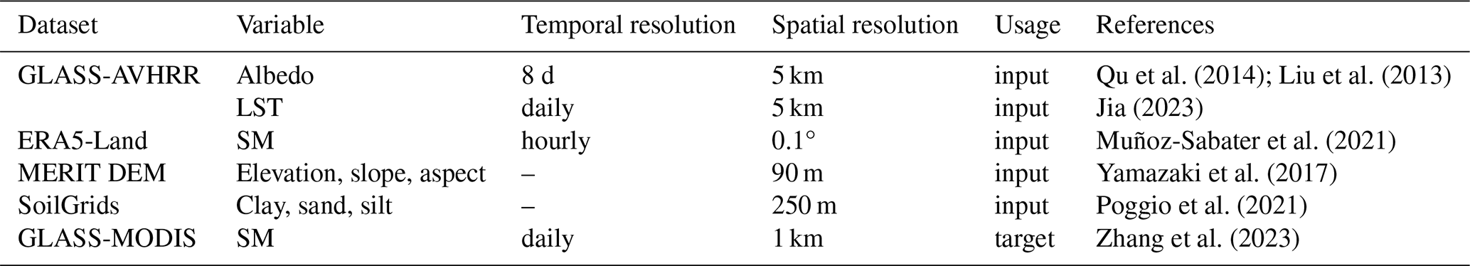
The multi-source datasets used in this study to develop the long-term SM estimation model are summarized in Table 2. The input variables were extracted from the GLASS-AVHRR albedo and LST products, the ERA5-Land reanalysis SM product, the Multi-Error-Removed Improved-Terrain (MERIT) digital elevation model (DEM), and the SoilGrids datasets, while the target variable was obtained from the GLASS-MODIS SM product. These input features are widely used in machine-learning-based and DL-based SM estimation studies. This section also introduces the ISMN, COsmic-ray Soil Moisture Observing System (COSMOS), and SMAP core validation sites (CVSs) in situ SM datasets used for validation, alongside the long-term ESA CCI SM product used for intercomparison.

Table 2 Summary of the multi-source datasets used to develop the long-term SM product.

2.1 GLASS-AVHRR albedo and LST products

As part of the GLASS product suite, the GLASS-AVHRR albedo and LST products were generated mainly from the long-archived AVHRR satellite observations dating back to the 1980s and are characterized by long-term temporal coverage, spatial continuity, and high accuracy (Liang et al., 2021). In particular, the GLASS-AVHRR albedo product was retrieved through a direct estimation algorithm (Qu et al., 2014) and a spatiotemporal filtering algorithm (Liu et al., 2013). The latest version (V5) of the GLASS-AVHRR albedo product at 5 km spatial resolution can be downloaded from http://www.glass.umd.edu/Albedo/MIX/ (last access: 18 September 2025). Here, the black-sky visible, near-infrared, and shortwave albedo were extracted and used as input variables, with the original 8 d temporal resolution interpolated to daily using linear interpolation to align with the training target. Meanwhile, the global all-sky GLASS-AVHRR LST product was estimated using a surface-energy-balance-based algorithm (Jia, 2023; Jia et al., 2024), which will be released soon. The daily mean LST at 5 km resolution was also used here as an input variable.

2.2 ERA5-Land SM product

ERA5-Land is a state-of-the-art long-term reanalysis dataset that includes multiple variables related to water and energy cycles spanning from 1950 to the present (Muñoz-Sabater et al., 2021). It offers seamless global coverage with an hourly temporal resolution and 0.1° spatial resolution. Previous validation studies show that although it typically exhibited high temporal correlations with in situ SM datasets, it often suffered from large biases (Gao et al., 2022; Xing et al., 2023; Zheng et al., 2022). Here, the first-layer (0–7 cm) ERA5-Land SM product was downloaded from https://cds.climate.copernicus.eu/ (last access: 18 September 2025). The daily mean SM was then calculated and up-sampled to 5 km through bilinear interpolation before being used as an input variable for the model to provide SM background information. Moreover, the ERA5-Land SM product was validated against in situ SM datasets and intercompared with the generated GLASS-AVHRR SM product.

2.3 Terrain and soil texture datasets

Topography and soil properties are the main factors that affect the spatial distribution of SM at fine scales. Here, we used the MERIT DEM (http://hydro.iis.u-tokyo.ac.jp/~yamadai/MERIT_DEM/, last access: 18 September 2025), a high-accuracy DEM generated by integrating multiple spaceborne DEMs (Yamazaki et al., 2017). This dataset covers 90° N–60° S over land at a resolution of 90 m and shows significant improvement in flat regions compared to previous spaceborne DEMs. After downloading the MERIT DEM, it was then used to derive elevation, slope, and aspect. Meanwhile, we also used the 250 m SoilGrids product (https://www.isric.org/explore/soilgrids, last access: 18 September 2025), a high-resolution soil property dataset generated from global soil profiles and environmental variables using machine learning models (Poggio et al., 2021). Specifically, the mean sand, silt, and clay content of the top soil layer (0–5 cm) were extracted from the SoilGrids product. All of these terrain and soil texture variables were resampled to 5 km before being used as inputs to the SM estimation model.

2.4 GLASS-MODIS SM product

The training target used in this study was the global 1 km spatiotemporally continuous GLASS-MODIS surface SM product (0–5 cm), which was generated using an XGBoost machine learning model that integrated the GLASS-MODIS albedo, LST, and leaf area index (LAI) products with multi-source datasets. In situ SM from the representative ISMN stations distributed globally was utilized by the XGBoost model as the training target (Zhang et al., 2023). This product exhibits high spatial and temporal consistency with both the ESA CCI and SMAP/Sentinel-1 L2 Radiometer/Radar SM products while maintaining a more complete spatial coverage. The daily GLASS-MODIS SM product from 2000 to 2020 is freely available at https://glass.hku.hk/archive/SM/MODIS/ (last access: 18 September 2025). Here, we derived training samples from the 5 km resampled GLASS-MODIS SM product rather than directly using in situ SM as the training target, as the global SM product could provide a much richer and representative training set than the sparse ISMN SM dataset.

2.5 In situ SM datasets

After generating the GLASS-AVHRR SM product using the developed DL model, three types of in situ SM datasets at different spatial scales were adopted to evaluate its accuracy and consistency. The characteristics of these in situ SM datasets are listed in Table 3, and the spatial distribution of the corresponding SM stations is shown in Fig. A1. The first type is the point-scale ISMN SM dataset (Dorigo et al., 2021), providing a valuable reference for validating gridded SM products, despite the relatively poor spatial representativeness of some SM stations. There were 1672 ISMN stations available for validation during Period I (2000–2018). Among them, 715 spatially representative stations were selected using the triple collocation method, as described in detail in Zhang et al. (2023). Although SM datasets from these representative stations were previously used as the target to train the GLASS-MODIS SM estimation model, making them only partially independent, they can be used here to assess the consistency between the GLASS-AVHRR and GLASS-MODIS SM products. Moreover, the 45 fully independent ISMN stations from Period II (1982–1999) can be used to evaluate the accuracy of the GLASS-AVHRR SM product during the earlier years. The daily mean SM was calculated by averaging the hourly SM measurements at the top soil layer (0–5 cm) obtained from https://ismn.earth/ (last access: 18 September 2025), considering only those flagged as “G” for good quality.

Table 3 Characteristics of three types of in situ SM datasets used in this study at different spatial scales.

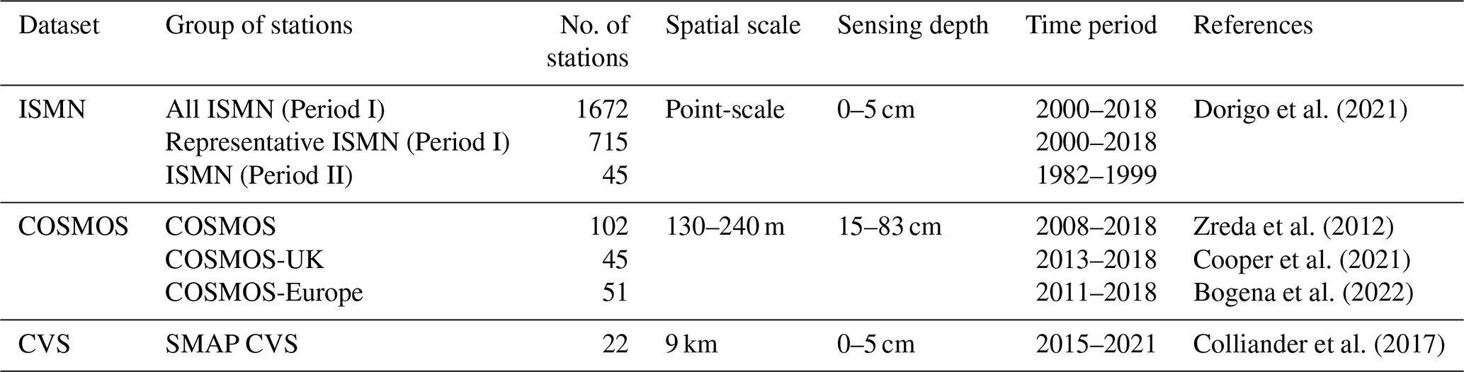
The second type is the COsmic-ray Soil Moisture Observing System (COSMOS) SM dataset, which includes area-averaged SM measurements at the field scale from three COSMOS networks: COSMOS (Zreda et al., 2012), COSMOS-UK (Cooper et al., 2021), and COSMOS-Europe (Bogena et al., 2022). The COSMOS sensors detect low-energy cosmic-ray neutrons above the ground, which can be converted to SM within a footprint radius of 130–240 m and a penetration depth of up to 83 cm, depending on factors such as air humidity, SM, and vegetation (Köhli et al., 2015). Although data from the COSMOS and COSMOS-UK networks had been integrated into the ISMN database, they were excluded from the training dataset of the GLASS-MODIS SM estimation model because their observation depths exceeded the 5 cm threshold. Recently, data from the COSMOS-Europe network have been released and can be accessed at https://doi.org/10.34731/x9s3-kr48. Collectively, these post-2000 SM datasets can serve as an independent source for validating the GLASS-AVHRR SM product at an intermediate scale. After filtering based on the quality flags and aligning with the GLASS-AVHRR SM product, there were 102 COSMOS, 45 COSMOS-UK, and 51 COSMOS-Europe stations available for validation. The distribution of sensing depths for each station across the three COSMOS networks is presented in Fig. A2. While COSMOS sensors measure SM at relatively deeper layers, they have been used to validate microwave and modeled surface SM products and show good correlations with them (Montzka et al., 2017; Peng et al., 2021b).

The third type is the SMAP/in situ core validation site (CVS) match-up dataset, which contains the upscaled in situ SM measurements derived from multiple quality-controlled stations that have been aligned with the SMAP SM products (Colliander et al., 2017). A total of 22 globally distributed CVSs were matched with the SMAP-Sentinel L2 SM product gridded at 9 km resolution (SMAPL2SMSP9 km). This independent 9 km SMAP CVS in situ dataset can be used to validate the GLASS-AVHRR SM product with reduced impact of scale difference. It covers the period from 2015 to the present and can be downloaded from https://nsidc.org/data/nsidc-0712/versions/1 (last access: 18 September 2025).

2.6 ESA CCI SM product

The European Space Agency (ESA) launched the Climate Change Initiative (CCI) SM project to develop the ESA CCI SM dataset, a global daily multi-decadal dataset aimed at supporting climate research (Dorigo et al., 2017). This dataset merged multiple microwave SM products into active-only, passive-only, and combined active–passive products, respectively. Here, we used the ESA CCI SM v7.1 combined product at a resolution of 0.25° (https://climate.esa.int/en/projects/soil-moisture/data/, last access: 18 September 2025), which covers the period 1978–2021. Despite being the most widely used long-term satellite SM product, it suffers from spatial incompleteness due to the lack of satellite observations in the earlier years, the observation gaps in satellite orbits, and the physical limitations of microwave observations for SM retrieval over densely vegetated areas (Dorigo et al., 2017). In this study, the spatial consistency between the ESA CCI combined SM product and our GLASS-AVHRR product was investigated.

3 Methods

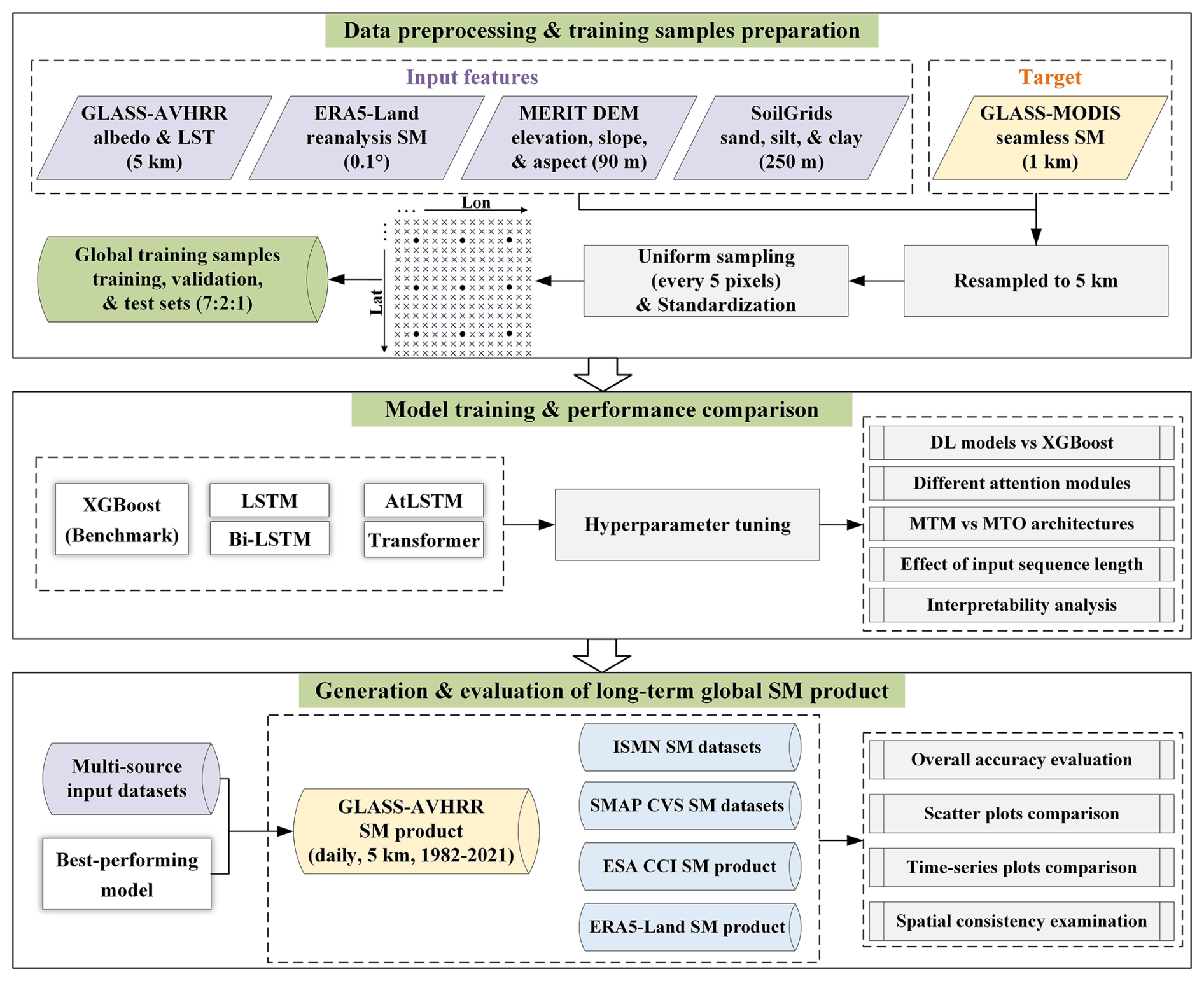
Figure 1 shows the flowchart of the proposed long-term global GLASS-AVHRR SM estimation framework, which consists of three main parts: data preprocessing and training sample preparation, model training and performance comparison, and generation and evaluation of the GLASS-AVHRR SM product.

Figure 1 Flowchart of the proposed long-term global GLASS-AVHRR SM estimation framework.

3.1 Training samples

The global GLASS-MODIS SM product resampled at 5 km was used as the training target of the long-term SM estimation model, from which a large number of representative and evenly distributed training samples could be obtained. Considering that the size of training samples would be too large if all the pixels were included, these samples were selected at 25 km (5 pixels) intervals along both the longitude and latitude, and a total of 135 360 pixels were chosen after excluding those with a large proportion of missing values. Based on the geographic coordinates of these pixels, the values corresponding to each input feature as well as the target SM for the years 2005, 2010, and 2015 were extracted, which collectively formed the time-series training samples. While the three years were selected to represent different periods within the available time span (2000–2020), this selection may introduce some uncertainty, as climate and environmental conditions can vary annually, and extreme weather or climate events in certain years may affect the representativeness of variables such as LST and SM. Nevertheless, this approach was adopted to control the sample size while ensuring the representativeness of samples across different years. These samples were then randomly divided into training, validation, and test datasets at a ratio of $\mathrm{7}:\mathrm{2}:\mathrm{1}$ based on their locations, ensuring spatial independence, with distances between any two samples exceeding 25 km, thereby minimizing the influence of spatial autocorrelation. While the training and validation datasets were used to train and tune the hyperparameters of the models, the accuracy of the models was evaluated on the test dataset. Figure 2 clearly illustrates the process of constructing time-series input samples for the DL models. Note that the input features need to be scaled before training a DL model, which helps to speed up the convergence process, avoids bias towards larger-scale features, and improves the model stability. Here, each input feature was standardized by subtracting the mean and then dividing by the standard deviation, whereas for the target SM, no further processing is needed because it is, by definition, scaled.

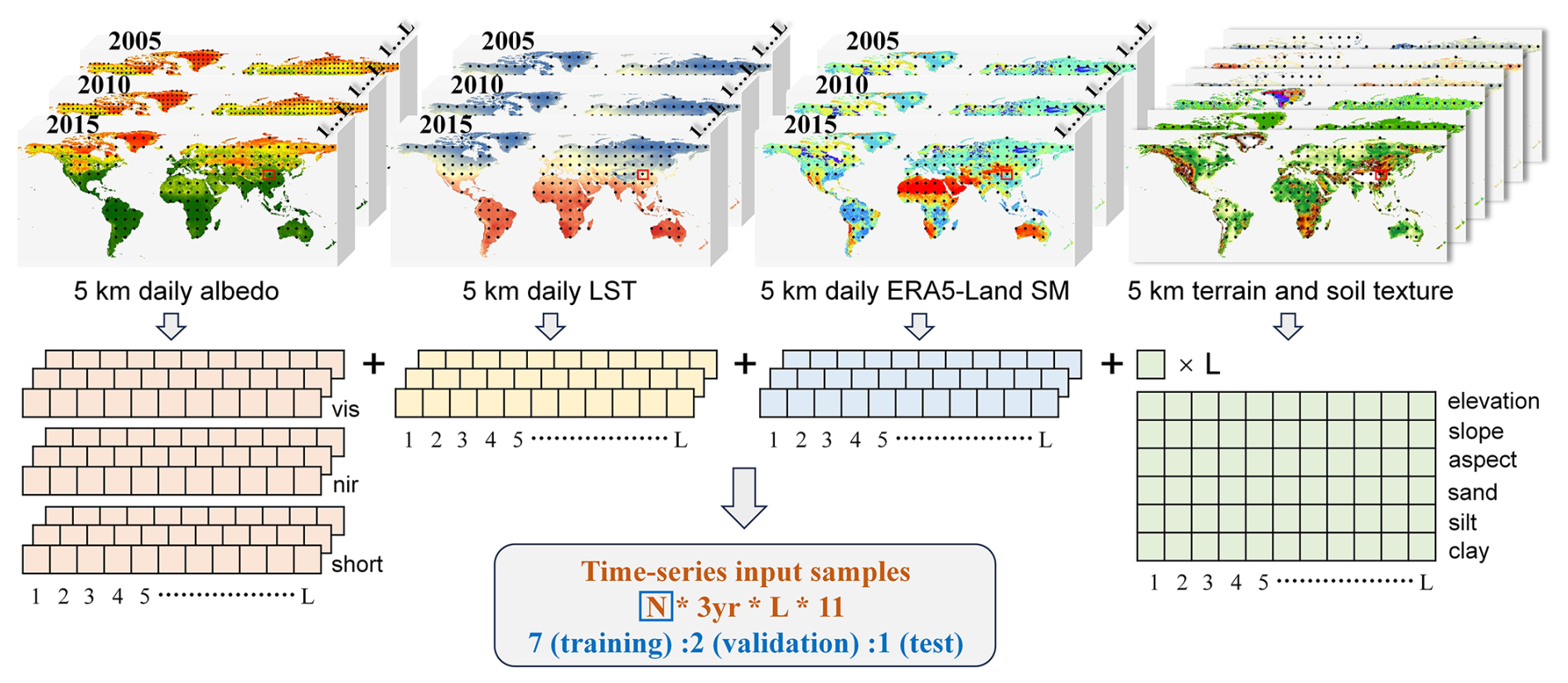
Figure 2 Schematic diagram illustrating the construction of time-series input samples for the DL models. N denotes the total number of samples, and L represents the sequence length, a hyperparameter that needs to be tuned.

3.2 Benchmark model

When generating the global 1 km GLASS-MODIS SM product, an XGBoost model was employed to integrate the multi-source datasets because of its good performance and high training and predicting speed. Here, we used the XGBoost model as a benchmark and compared its performance with the DL models (LSTM-based and transformer) to analyze whether the DL models exhibit an advantage over this widely used machine learning model in SM estimation. The XGBoost model (Chen and Guestrin, 2016) is a type of gradient boosting model, in which multiple trees are iteratively constructed through correcting the prediction residuals of the preceding trees. A schematic diagram of the XGBoost model is shown in Fig. 3e, where predictions from multiple trees are combined to make the final SM prediction. The key hyperparameters were configured as follows: n_estimators=1000, learning_rate=0.1, and max_depth=8. The time-series training samples constructed above were put together to train the XGBoost model, and the overall accuracy achieved by the XGBoost model on the test dataset was then compared with that of the DL models as a benchmark.

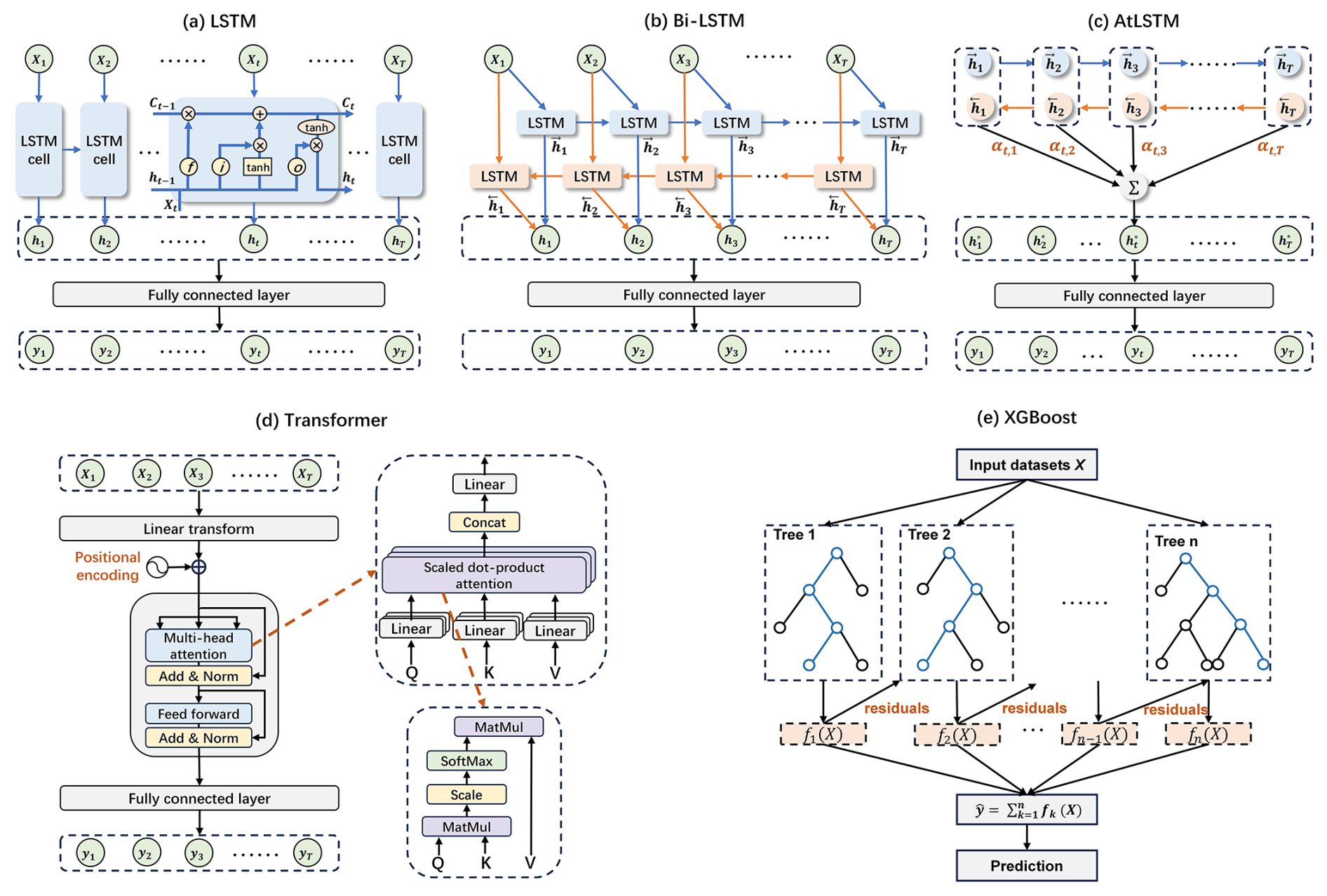
Figure 3 Schematic diagrams of the five models used in this study: (a) LSTM, (b) Bi-LSTM, (c) AtLSTM, (d) transformer, and (e) XGBoost. In subplots (a–d), x_t, y_t, and h_t represent the input datasets, SM prediction, and hidden state output by the models at time step t, respectively.

3.3 Models based on long short-term memory

The LSTM network (Hochreiter and Schmidhuber, 1997) is a special type of recurrent neural network (RNN) designed to solve the problems of gradient vanishing and exploding when training long sequences. The basic LSTM network introduces the memory cell, which is a special type of hidden state that shares the same shape as the hidden state but is designed to record long-term information. Each recurrent unit within the LSTM has three distinct gates, i.e., the forget gate, input gate, and output gate, as illustrated in Fig. 3a. The formulas used to calculate the three gates (f_t, i_t, o_t), cell state (c_t), and hidden state (h_t) are given below:

$$\begin{array}{}\text{(1)}& {\displaystyle }& {\displaystyle }{f}_t=\mathit{\sigma }(W_f.[h_{t-\mathrm{1}},x_t]+b_f),\text{(2)}& {\displaystyle }& {\displaystyle }{i}_t=\mathit{\sigma }(W_i.[h_{t-\mathrm{1}},x_t]+b_i),\text{(3)}& {\displaystyle }& {\displaystyle }{o}_t=\mathit{\sigma }(W_o.[h_{t-\mathrm{1}},x_t]+b_o),\text{(4)}& {\displaystyle }& {\displaystyle }{c}_t=f_t\ast c_{t-\mathrm{1}}+i_t\ast \tanh (W_c.[h_{t-\mathrm{1}},x_t]+b_c),\text{(5)}& {\displaystyle }& {\displaystyle }{h}_t=o_t\ast \tanh \left(c_t\right),\end{array}$$

where x_t represents the input datasets at time step t and h_t−1 is the hidden state at the previous time step; f_t, i_t, and o_t are all calculated as linear functions of x_t and h_t−1 with different weights and biases and are then rescaled using a non-linear sigmoid (σ) function. The σ function acts as the gating function for the three gates, with an output ranging between 0 and 1, thereby determining which portion of the information passes through the gates. Both the σ and tanh functions add non-linearity to the LSTM network. The bidirectional LSTM (Bi-LSTM) extends the LSTM network by incorporating both forward and backward LSTM units within a single layer, allowing the model to capture contextual information from both directions before concatenating their outputs. As displayed in Fig. 3b, the Bi-LSTM model can learn bidirectional (preceding and following) information at each time step.

The LSTM network has different architectures, including many-to-one (MTO) and many-to-many (MTM). In research areas like crop mapping and runoff prediction, the MTO architecture is primarily adopted, which uses inputs from multiple time steps to output estimates for a single time step. Alternatively, we adopted the MTM architecture, which takes time-series inputs and outputs SM estimates for all time steps simultaneously by feeding the hidden states from all time steps into a fully connected layer. We also conducted an experiment to compare the estimation accuracy of these two architectures.

In addition to the basic LSTM and Bi-LSTM networks introduced above, an attention module was added to the Bi-LSTM network, referred to as the AtLSTM network, to explore if the estimation accuracy of SM could be further improved. The AtLSTM network was constructed based on Bahdanau et al. (2014) and Xu et al. (2020) and adapted here for the MTM architecture. As illustrated in Fig. 3c, the attention module generates the attention weights (α), which are then multiplied with the hidden states (h) to get the weighted hidden states (h^∗). α and h^∗ can be calculated as follows:

$$\begin{array}{}\text{(6)}& {\displaystyle }& {\displaystyle }{e}_t=W_a.h_t+b_a,\text{(7)}& {\displaystyle }& {\displaystyle }{\mathit{\alpha }}_{t,i}=\text{softmax}\left(e_{t,i}\right)={\displaystyle \frac{\exp \left(e_{t,i}\right)}{{\sum }_{j=\mathrm{1}}^T\exp \left(e_{t,j}\right)}},\text{(8)}& {\displaystyle }& {\displaystyle }{h}_t^{\ast }=\sum _{i=\mathrm{1}}^T{\mathit{\alpha }}_{t,i}\ast h_i,\end{array}$$

where W_a and b_a denote the learnable parameters that map the hidden states h into a weight matrix e and T is the sequence length of the input features. The weight matrix (with the shape of T×T) is then rescaled by a softmax function to obtain the attention weights for each hidden state, which range between 0 and 1 and sum to 1. The weighted hidden states h^∗ are then fed into a fully connected layer to estimate the target variable. Intuitively, higher attention weights indicate that the corresponding hidden states have a greater influence on the estimation of SM at a specific time step.

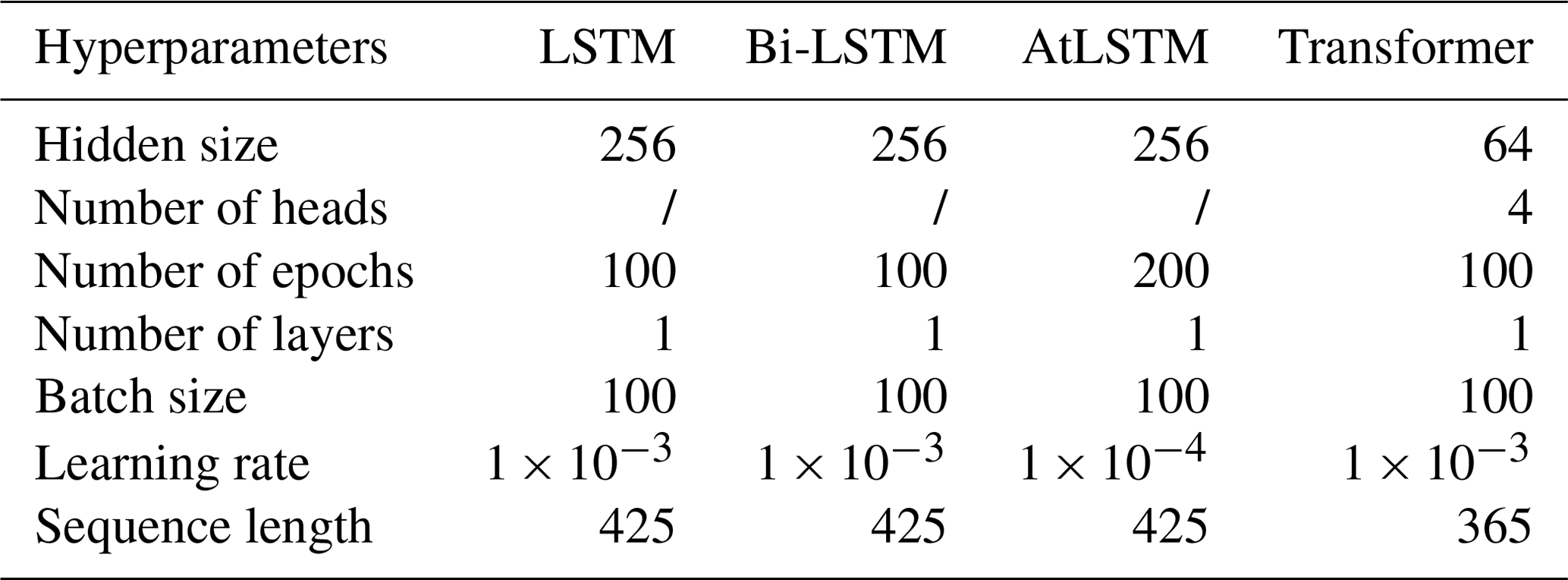
In this study, the LSTM-based models were implemented using the open-source PyTorch 2.0 framework. The mean square error (MSE) was used as the loss function, and the Adam optimizer was adopted to update the learnable parameters of the models. Several key hyperparameters were tuned, including the hidden size, number of epochs, and learning rate (Zhang et al., 2021). For each model, the hidden size was determined after testing values of 64, 128, 256, and 512; the number of epochs, after testing 20, 50, 100, and 200; and the learning rate, after testing 0.1, 0.01, 0.001, and 0.0001. The final settings of the major hyperparameters for the three LSTM-based models are listed in Table 4.

Table 4 Key hyperparameters configured for the DL models used in this study.

3.4 Transformer

The transformer network is a DL architecture based entirely on attention mechanisms, dropping the recurrent structure to avoid the constraint of sequential calculation. After being proposed by Vaswani et al. (2017), transformer soon become the state-of-the-art model for natural language processing and has also been applied successfully to areas like computer vision (Dosovitskiy et al., 2020) and time-series analysis (Wen et al., 2022). Its core component is the multi-head self-attention layers, which can relate any two positions in a sequence. More specifically, multi-head attention involves applying the attention function to multiple sets of key, value, and query vectors in parallel, thus enabling the model to focus on different parts of the input sequence simultaneously. Unlike the attention function used in the AtLSTM model (Eqs. 6–7), transformer uses the scaled dot-product attention α, which can be calculated as follows:

$$\begin{array}{}\text{(9)}& \mathit{\alpha }(Q,K,V)=\text{softmax}\left({\displaystyle \frac{Q{K}^T}{\sqrt{d_k}}}\right)V,\end{array}$$

where Q, K, and V refer to the query, key, and value vectors, respectively, which are derived by multiplying the embedded input sequence with the corresponding learnable projection matrix, and d_k is the dimension of the key and query vectors. Additionally, with the help of a positional encoding function, the transformer network can retain some ordinal information for elements in the input sequence. A detailed description of transformer and the multi-head self-attention mechanism can be found in Vaswani et al. (2017). Compared with recurrent or convolutional neural networks, the transformer network can efficiently parallelize much larger amounts of computation and capture long-range dependencies in the input sequence more easily. Here, we used only the encoder portion of the original transformer network to map the input features into hidden representations, which were then fed into a fully connected layer to output the time-series SM estimates (Fig. 3d). The same training samples, optimizer, and loss function used for the LSTM-based models were employed to train the transformer network, with the settings of its hyperparameters also listed in Table 4. Notably, the number of heads is a unique hyperparameter of transformer that refers to the number of parallel self-attention layers of the encoder.

3.5 Evaluation of the models and GLASS-AVHRR SM product

After training the benchmark XGBoost model and the four DL models described above using the same training samples distributed worldwide, their performances on the test set were then compared from multiple perspectives, including comparisons between the DL models and XGBoost model, between the DL models with different attention mechanisms, and between the DL models with MTM or MTO architectures. Moreover, the effect of the input sequence length on model accuracy was investigated using the LSTM-based models, and a preliminary interpretability analysis was performed through visualizing the attention weights of both the AtLSTM and transformer models. Then, the best-performing model, along with the multi-source input datasets, was employed to generate the global daily GLASS-AVHRR SM product at 5 km resolution from 1982 to 2021. To fully assess the derived long-term SM product, different SM datasets and evaluation strategies were combined, including overall accuracy evaluation, scatter plot analysis, time-series plot comparison, and spatial consistency examination. Specifically, the accuracy of this product was first evaluated against the point-scale ISMN, field-scale COSMOS, and upscaled 9 km SMAP CVS in situ SM datasets, respectively. Then, the GLASS-AVHRR SM product was intercompared with the GLASS-MODIS SM product and two widely used long-term global SM products, namely, ERA5-Land and ESA CCI, to investigate their spatial consistency.

4 Results

4.1 Comparison of model performance

Table 5 lists the performance metrics achieved by the benchmark tree-based XGBoost model and four DL models on the training set, validation set, and two types of test sets, respectively. The XGBoost model achieved similar overall accuracy across the training, validation, and test sets, with a coefficient of determination (R²) of 0.984 and RMSE of 0.012 m³ m⁻³ on the training set and an R² of 0.982 and RMSE of 0.013 m³ m⁻³ on both the validation and test sets, indicating a low tendency for overfitting. The fairly high overall accuracy of the benchmark XGBoost model may be attributed to the large number of training samples, specifically 135 360 pixels per day over 3 years, evenly distributed across the globe on a daily basis. To evaluate the impact of sample size on model performance, we conducted an experiment by reducing the number of training samples. When the sample size was reduced by a factor of 100, the accuracy of the XGBoost model dropped considerably, with an R² of 0.96 and RMSE of 0.017 m³ m⁻³ on the test set. This highlights the importance of having sufficient samples to achieve high accuracy with XGBoost and indicates the advantage of using the GLASS-MODIS SM product as the training target, which can provide much richer samples than the sparse in situ ISMN SM dataset. Meanwhile, Table 5 also shows that the accuracy of the XGBoost model decreases drastically on the test set with SM observations exceeding 0.4 m³ m⁻³, yielding an R² of 0.413 and RMSE of 0.022 m³ m⁻³, likely due to the relatively smaller portion of samples at high SM levels.

Table 5 Performance metrics of the benchmark XGBoost model and four DL models on the training set, validation set, and two types of test sets.

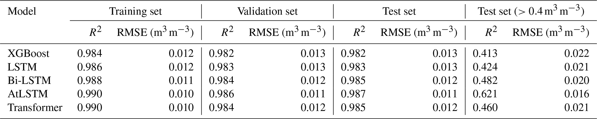
In comparison, the LSTM model developed using time-series training samples performed slightly better than the XGBoost model, with the R² on the test set increasing to 0.983, and when the Bi-LSTM model was employed, the overall accuracy on the test set was further improved, with the R² increasing to 0.985 and RMSE decreasing to 0.012 m³ m⁻³. Although the increase in the overall accuracy might not be significant, the Bi-LSTM model exhibited significant improvement over the XGBoost model at high SM levels, achieving an R² of 0.482 and RMSE of 0.020 m³ m⁻³ on the test set for observations exceeding 0.4 m³ m⁻³. As also can be seen from the density scatter plots in Fig. 4, the majority of samples had SM values below 0.4 m³ m⁻³ (indicated by the red dots), where all models achieved high prediction accuracy. However, on the relatively infrequent samples with high SM values, where the XGBoost model tended to yield lower estimates, both the LSTM and Bi-LSTM models provided more accurate estimates. Given the temporal autocorrelation of SM, these results suggest that learning both forward and backward temporal information from the time-series training samples enhances the ability of DL models to estimate SM more accurately, especially at high SM levels with sparser samples.

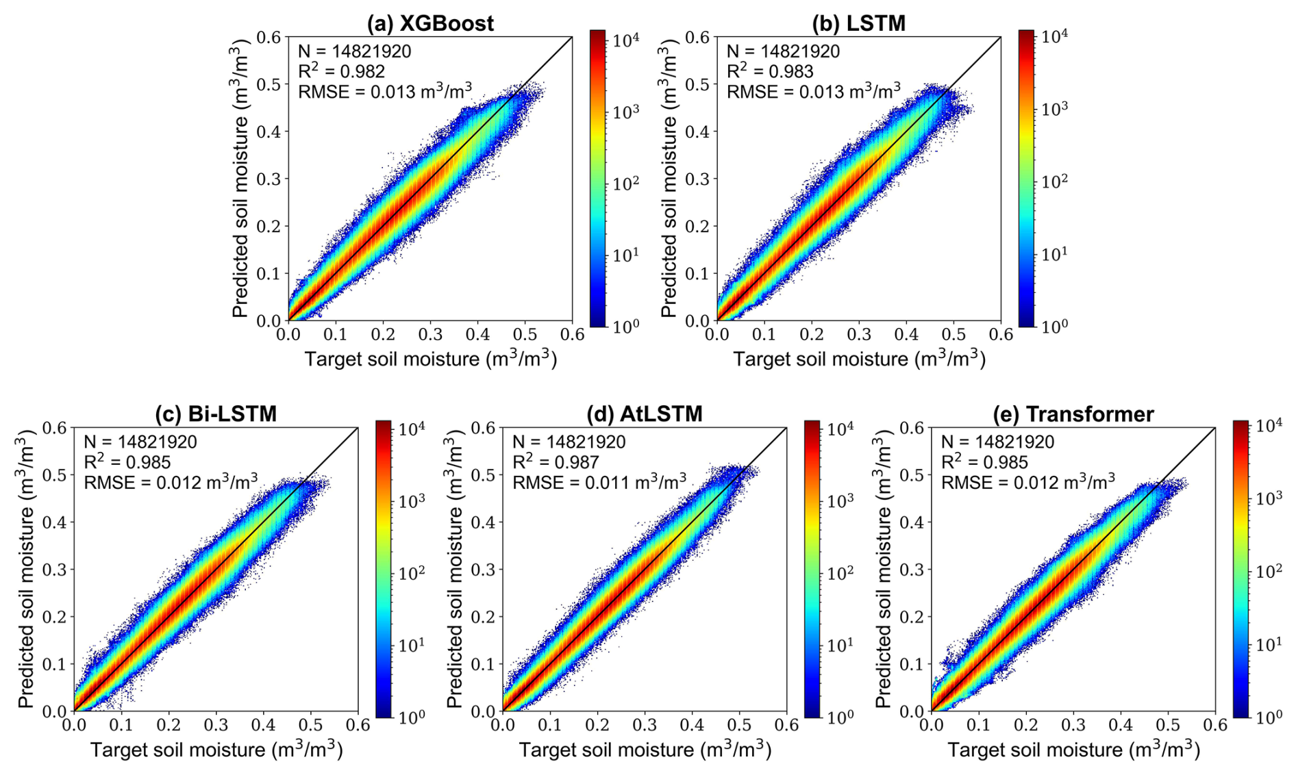
Figure 4 Scatter plots between target SM and predicted SM for the (a) XGBoost, (b) LSTM, (c) Bi-LSTM, (d) AtLSTM, and (e) transformer models on the test set. The colors of the dots indicate different probability densities, and the black line represents the 1:1 line.

Then, after adding the attention module into the Bi-LSTM model, the derived AtLSTM model achieved the best performance, with an R² of 0.987 and RMSE of 0.011 m³ m⁻³ on the test set. In contrast, despite the fact that the transformer model also incorporated an attention module, its accuracy was slightly lower than that of the AtLSTM model on the test set and significantly lower on samples with high SM levels ($>\mathrm{0.4}{\mathrm{m}}^{\mathrm{3}}{\mathrm{m}}^{-\mathrm{3}}$) in our experiments. As mentioned above, the main advantage of the transformer model is its ability to capture long-range dependencies and handle long sequences effectively. However, soil moisture often exhibits high temporal variability, meaning it can change rapidly due to factors such as rainfall and evaporation. In this context, short-term adjacent temporal information can be critical for accurate SM estimation. The slightly better performance of the AtLSTM model compared with the transformer model may be attributed to its superior ability to capture these short-term adjacent dependencies, which are critical for modeling the nuances in rapidly changing SM levels. This will be further investigated through the analysis of attentional weights below. Additionally, a feature importance analysis was conducted for the best-performing AtLSTM model, as shown in Fig. A3. Specifically, the gradients of the model's output with respect to each input feature were computed on the test set, and the absolute values of these gradients were then averaged across all samples and time steps. Input features with larger average gradients are considered to exert a more significant influence on the model's predictions. The results indicate that elevation, black-sky visible albedo, ERA5-Land reanalysis SM, and slope are the most influential features for the AtLSTM model. In particular, although elevation is a static variable, it plays a critical role in shaping the spatial distribution of SM by influencing precipitation, temperature, vegetation type, and evaporation processes. Its impact on the spatial variability of SM tends to be more stable and consistent over time. In contrast, the contributions of dynamic input features such as ERA5-Land SM may fluctuate across time and space and can be diminished by inherent uncertainties and biases in the input data. Moreover, their importance may be influenced by correlations with other input features. To further investigate the importance of multi-source datasets for the performance of the AtLSTM model, we conducted ablation experiments by individually removing the ERA5-Land SM and the GLASS-AVHRR albedo and LST products from the input datasets. The results show that the AtLSTM model's accuracy on the test set decreased significantly, with R² dropping to 0.954 and 0.968 and RMSE increasing to 0.020 and 0.018 m³ m⁻³, respectively. These results demonstrate that by integrating multi-source datasets and leveraging their complementary strengths, the AtLSTM model can achieve substantially improved accuracy in long-term SM estimation.

While the numerical differences in overall accuracy among all these models may not seem remarkable, a more intuitive comparison can be drawn from their density scatter plots. As shown in Fig. 4, on the majority of samples, both the best-performing AtLSTM model and benchmark XGBoost model can achieve high prediction accuracy, resulting in a relatively small difference in their overall performance on the test set. However, there remains a small portion of samples that are more challenging to predict, on which the SM estimates from the AtLSTM model are much closer to the 1:1 line compared with the XGBoost model. Furthermore, the AtLSTM model significantly improves upon the tendency of the XGBoost model to produce lower estimates at high SM levels, achieving an R² of 0.621 and RMSE of 0.016 m³ m⁻³ on the test set for observations exceeding 0.4 m³ m⁻³. Overall, while both the XGBoost model and the four DL models can achieve high SM estimation accuracy, the AtLSTM model yields the highest accuracy among them and performs well across different SM levels, with a low tendency for overfitting. This suggests that utilizing bidirectional temporal information from the input sequence and adding an attention module are both effective in further improving the estimation accuracy of SM.

As mentioned in Sect. 3.3, we chose to use the MTM architecture when developing the DL models to output time-series SM estimates at once. Here, to compare the accuracy of the MTM architecture with the more commonly used MTO architecture, as well as to investigate the effect of input sequence length on model accuracy, we calculated performance metrics for the LSTM models utilizing these two different architectures under varying lengths of input sequences. Specifically, both types of models were trained using input features from a given date (e.g., the first day of 2015) and n days (0–29) prior to that date, respectively, and the accuracy of the models was then evaluated on the test set for that given date. To reduce the training time, the number of epochs for these LSTM models was set to 20. It can be seen from the R² and RMSE curves in Fig. 5a that as the length of the input sequence increased, the accuracy of the LSTM model with the MTO architecture also increased, and then the accuracy leveled off at a sequence length of about 10 d. This indicates that while accounting for temporal information can be beneficial for current SM estimation, only the most recent input sequences have a remarkable effect on the model's accuracy. In comparison, the LSTM model with the MTM architecture, which can output a sequence of SM estimates simultaneously, achieved similar accuracy to that of the MTO architecture, and its R² and RMSE curves stabilized at a sequence length of about 5 d. This demonstrates the feasibility of adopting the MTM architecture in the LSTM model, which not only considerably reduces the production time but also maintains the estimation accuracy.

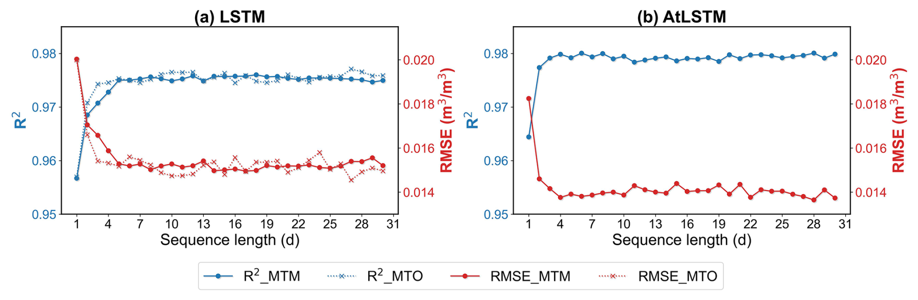
Figure 5 Performance metrics of (a) the LSTM models with two different types of architectures (MTO and MTM) and (b) the AtLSTM model with the MTM architecture, trained using varying lengths of input sequences on the test set. The blue and red curves represent the R² and RMSE curves, respectively.

Moreover, we also investigated the effect of the input sequence length on the overall accuracy of the AtLSTM model with the MTM architecture, and the performance metrics were calculated here based on SM estimates over the entire time series instead of on a given date. To reduce the training time and account for the smaller learning rate used for the AtLSTM model (Table 4), the number of epochs was set to 50. As displayed in Fig. 5b, the overall accuracy of the AtLSTM model increased sharply as the length of the input sequence increased, and then the accuracy plateaued at a sequence length of about 4 d. The more rapid stabilization of the AtLSTM model's accuracy may be attributed to the incorporation of the Bi-LSTM module in the model, which can utilize both forward and backward temporal information. In addition, it seems that when the input sequence is long enough, the model can automatically learn the necessary temporal information to accurately estimate SM at each position in the sequence. However, it should be noted that at the beginning or end of the sequence, the model's accuracy tends to decrease, as only forward or backward information can be utilized, which is a common issue encountered by the LSTM-based models with the MTM architecture. Therefore, to facilitate the production process, the sequence length of the LSTM-based models was finally set to 425 d, and both the first 30 and last 30 values were discarded (a rather sufficient number) after the model output the time-series SM estimates so that an entire year's SM estimates could be obtained in a single run. Note that, during both the training and production phases, the first and last 30 d of each 425 d sequence were padded with actual data from adjacent years to ensure consistency.

Although data-driven DL models are commonly perceived as “black boxes”, there are many techniques that can be employed to increase the interpretability of DL models. In the case of attention-based deep neural networks, this can be achieved by analyzing the distribution of attention weights. In a long sequence, perhaps only a portion of the information is critical to the model prediction at a given time step, and the attention mechanism enables the model to focus on these critical positions. In particular, the attention module of the AtLSTM model can dynamically adjust the weights of the hidden states output by the model at each time step. Figure 6a illustrates the distribution of the averaged attention weights calculated using the best-performing AtLSTM model on the test set (40 608 samples). To show more detail, only the attention weights of 30 consecutive days selected from the entire sequence (425 d) are displayed here, and attention weights less than 0.0001 are masked out. It is observed that, for the hidden state at each time step in the sequence (vertical axis), the largest attention weight was located approximately 3 d around that time step (horizontal axis). This indicates that when the attention module of the AtLSTM model learns to readjust the hidden states, it primarily utilizes the temporal information from adjacent positions in the sequence.

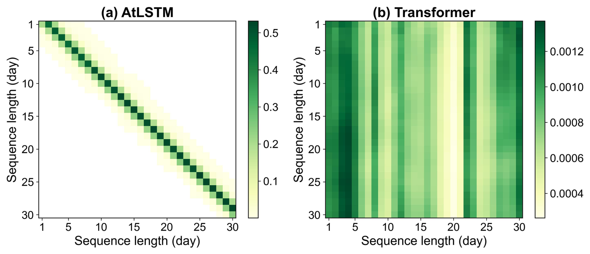
Figure 6 Heatmaps of the averaged attention weights calculated using the (a) AtLSTM and (b) transformer model on the test set (40 608 samples). Only the attention weights of 30 consecutive days selected from the entire sequence are displayed here for illustration.

In contrast, as a core component of the transformer model, the multi-head self-attention layers can capture various aspects of relationships between different positions within a sequence, and the attention weights generated by these layers are then directly applied to the embedded input sequence. Figure 6b shows, as a comparison, the distribution of attention weights calculated by averaging the outputs from the four attention heads of the transformer model. The attention weight heatmap of the transformer model is quite different from that of the AtLSTM model, with the weight at each position being much smaller and dispersed. This is likely because the self-attention module can relate any two positions in the sequence, and inputs from more distant positions may contribute more to the model output at the current time step. In addition, for each time step in the sequence (vertical axis), there were some common positions (horizontal axis) with larger weights that were more important for model prediction. Despite the distinct attention mechanisms employed by these two DL models, both of them achieved high SM estimation accuracy. Given that SM is temporally autocorrelated and highly variable over time, the slightly better performance of the AtLSTM compared to the transformer model may be attributed to the fact that it extracts temporal information mainly from adjacent positions in the sequence, rather than from more distant ones, for SM estimation.

4.2 Validation of the GLASS-AVHRR SM product

After generating the GLASS-AVHRR SM product using the best-performing AtLSTM model with the MTM architecture, permanent snow and ice as well as water bodies were masked out with the help of the MODIS land cover type product (MCD12C1) (Friedl and Sulla-Menashe, 2022). The derived SM product was then evaluated against three types of in situ SM datasets at different spatial scales. The first type is the point-scale ISMN SM dataset, which is distributed globally and covers a wide range of land cover types. There were 1672 ISMN stations and 715 spatially representative stations available for validation during Period I (2000–2018). The distribution of validation metrics achieved by the GLASS-AVHRR SM product on these partially independent ISMN stations during Period I, grouped by all stations and representative stations, is presented in Fig. 7, alongside those of the GLASS-MODIS and ERA5-Land SM products for comparison. The GLASS-AVHRR SM product achieved comparable performance to that of the GLASS-MODIS SM product across all ISMN stations and representative stations during Period I. In addition, both GLASS SM products performed significantly better at the representative stations. This demonstrates the high level of consistency in accuracy between the two GLASS SM products. Note that the validation metrics for the GLASS-MODIS product were derived using a site-independent cross-validation method, which was designed to accurately reflect the product's performance over unknown areas. Given the consistency in the distribution of validation metrics between the GLASS-AVHRR and GLASS-MODIS SM products, the accuracy achieved by the GLASS-AVHRR product at these partially independent stations should also approach its true accuracy. In contrast, although the ERA5-Land SM product achieved a similar distribution of R to the two GLASS SM products across all ISMN stations and representative stations, it exhibited much larger biases and ubRMSE values.

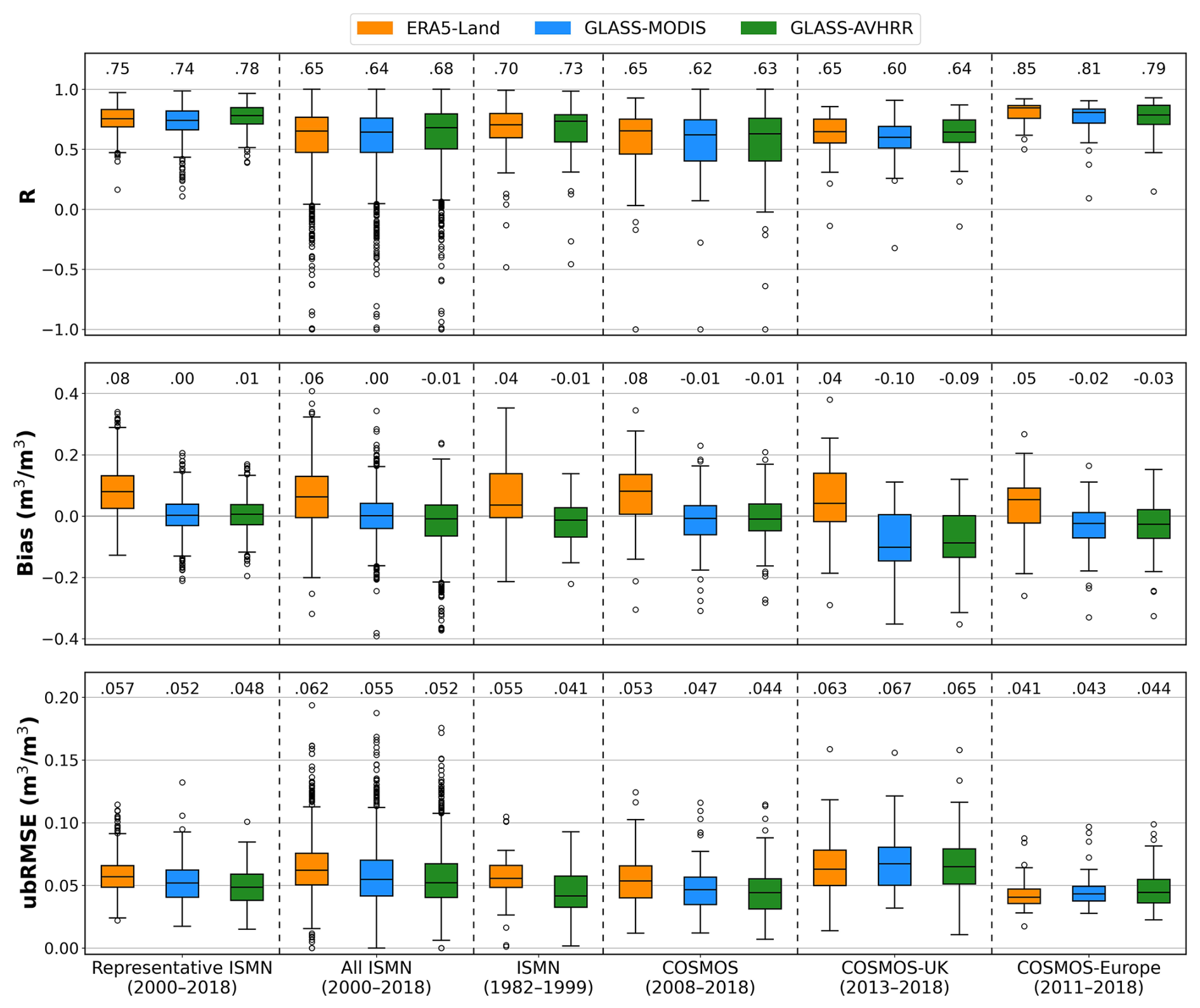
Figure 7 Boxplots of R, bias, and ubRMSE for the GLASS-AVHRR SM product across different groups of ISMN stations and three field-scale COSMOS networks, in comparison with the GLASS-MODIS and ERA5-Land SM products. The number above each box represents the median value of the metrics across all stations within each network.

To conduct a more independent evaluation of the GLASS-AVHRR SM product, the ISMN SM dataset from Period II (1982–1999) was also collected. After excluding stations that overlapped with the 715 representative stations from Period I, only 45 independent stations remained for evaluation during Period II. The observations at these stations were also quite limited; hence, the validation metrics derived from them may not provide a comprehensive assessment. Nevertheless, it can be seen from Fig. 7 that the GLASS-AVHRR product achieved rather high accuracy at these stations, with a median R of 0.73 and a median ubRMSE of 0.041 m³ m⁻³. Likewise, while the ERA5-Land SM product exhibited a similar distribution of R to the GLASS-AVHRR product at these stations, it achieved much larger biases and ubRMSE values. The second type of in situ SM dataset comprises field-scale measurements from three COSMOS networks, i.e., COSMOS, COSMOS-UK, and COSMOS-Europe, which can provide an independent evaluation of the GLASS-AVHRR SM product at an intermediate scale. As shown in Fig. 7, the GLASS-AVHRR, GLASS-MODIS, and ERA5-Land SM products all achieved good performance across the three COSMOS networks. The two GLASS SM products showed comparable overall accuracy across these networks, although some site-specific discrepancies were observed, which are likely due to differences in the satellite remote sensing inputs and spatial resolution. Yet, their accuracies varied considerably across these networks, with the median R ranging from 0.63 to 0.79 and the median ubRMSE ranging from 0.044 to 0.065 m³ m⁻³ for the GLASS-AVHRR product. This variability may be attributed to the different footprint radii of COSMOS sensors, which result in varying degree of spatial representativeness and spatial mismatches with gridded SM products. These factors can introduce uncertainty into the validation results, particularly affecting the bias and ubRMSE metrics. The biases of the GLASS-AVHRR SM product on the COSMOS-UK network were much larger than those on the other two COSMOS networks, with the median bias reaching $-\mathrm{0.09}{\mathrm{m}}^{\mathrm{3}}{\mathrm{m}}^{-\mathrm{3}}$. This is likely due to the greater sensing depth of the COSMOS-UK network, which has a median depth of 30 cm, compared to 21 and 22 cm for the COSMOS and COSMOS-Europe networks, respectively (Fig. A2). Moreover, both the GLASS-AVHRR and ERA5-Land SM products exhibited larger ubRMSE values on the COSMOS-UK network. This may be related to the increased uncertainty of COSMOS measurements in organic soils or humid regions, which are prevalent in the UK, as also reported by Zheng et al. (2024). Meanwhile, although the first-layer (0–7 cm) ERA5-Land SM product was used here for evaluation, it still exhibited large wet biases across these COSMOS networks, further suggesting its extensive overestimation issue.

Despite the high accuracy achieved when validating the GLASS-AVHRR SM product using both the point-scale ISMN and field-scale COSMOS in situ SM datasets, the validation results were inevitably affected by the scale differences between these datasets. Therefore, the upscaled 9 km SMAP CVS in situ SM dataset from 22 different locations was also utilized to validate the GLASS-AVHRR SM product from 2015 to 2021 as a complement. Specifically, the mean SM values of the 5 km GLASS-AVHRR SM product within a 2×2 window corresponding to each 9 km SMAP CVS grid were first calculated, and then the validation metrics for the GLASS-AVHRR SM product were estimated at each CVS, as listed in Table 6. As a comparison, validation metrics for the ERA5-Land SM product (∼9 km horizontal resolution) were also calculated at each CVS and are presented in the table.

Table 6 Validation metrics for the GLASS-AVHRR and ERA5-Land SM products at 22 upscaled 9 km SMAP core validation sites, with the best-performing metrics highlighted in bold.

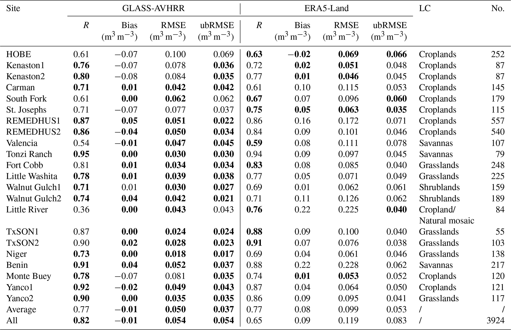
At most of the CVSs, the GLASS-AVHRR SM product achieved similar R values to the ERA5-Land SM product, except at the Little River site, where the R value for the GLASS-AVHRR product was significantly lower. This is probably because the land cover type at this site is “Cropland or Natural mosaic”, making the upscaled in situ SM measurements less representative and the validation results at this site less reliable. Meanwhile, while the GLASS-AVHRR SM product exhibited notable dry biases only at a few CVSs, the ERA5-Land SM product showed large wet biases at most of the CVSs, as also reported in detail by Lal et al. (2022). The varying degrees of bias in these two SM products can be more intuitively observed through their scatter plots against the upscaled in situ SM at each CVS (Fig. 8). As one of the main inputs for generating the GLASS-AVHRR SM product, the ERA5-Land reanalysis SM exhibited notable wet biases at almost all CVSs, especially at REMEDHUS1, Little River, and Benin, which were largely corrected by the GLASS-AVHRR product, with the data points on the scatter plots being much closer to the 1:1 line. This can be attributed to the use of the GLASS-MODIS SM product as the training target, although it may have also contributed to the slight dry bias in the GLASS-AVHRR SM product, given that optical and thermal satellite SM estimates typically represent a shallower depth than in situ SM datasets. In addition, at the CVS where the ERA5-Land product exhibited a large wet bias, the RMSE and ubRMSE values of the GLASS-AVHRR product were often much lower than those of the ERA5-Land product. The average R and ubRMSE values achieved by the GLASS-AVHRR SM product at 22 CVSs were 0.77 and 0.037 m³ m⁻³, respectively, similar to those reported for the 9 km SMAP-Sentinel L2 SM product, which were 0.79 and 0.035 m³ m⁻³, respectively (Das et al., 2020). When combining all the CVS in situ SM measurements, an overall R of 0.82 and ubRMSE of 0.054 m³ m⁻³ were obtained by the GLASS-AVHRR SM product, showing significant improvement over the ERA5-Land SM product, which had values of 0.65 and 0.083 m³ m⁻³, respectively. This is also evident from the more concentrated scatter points of the GLASS-AVHRR SM product displayed in Fig. 8.

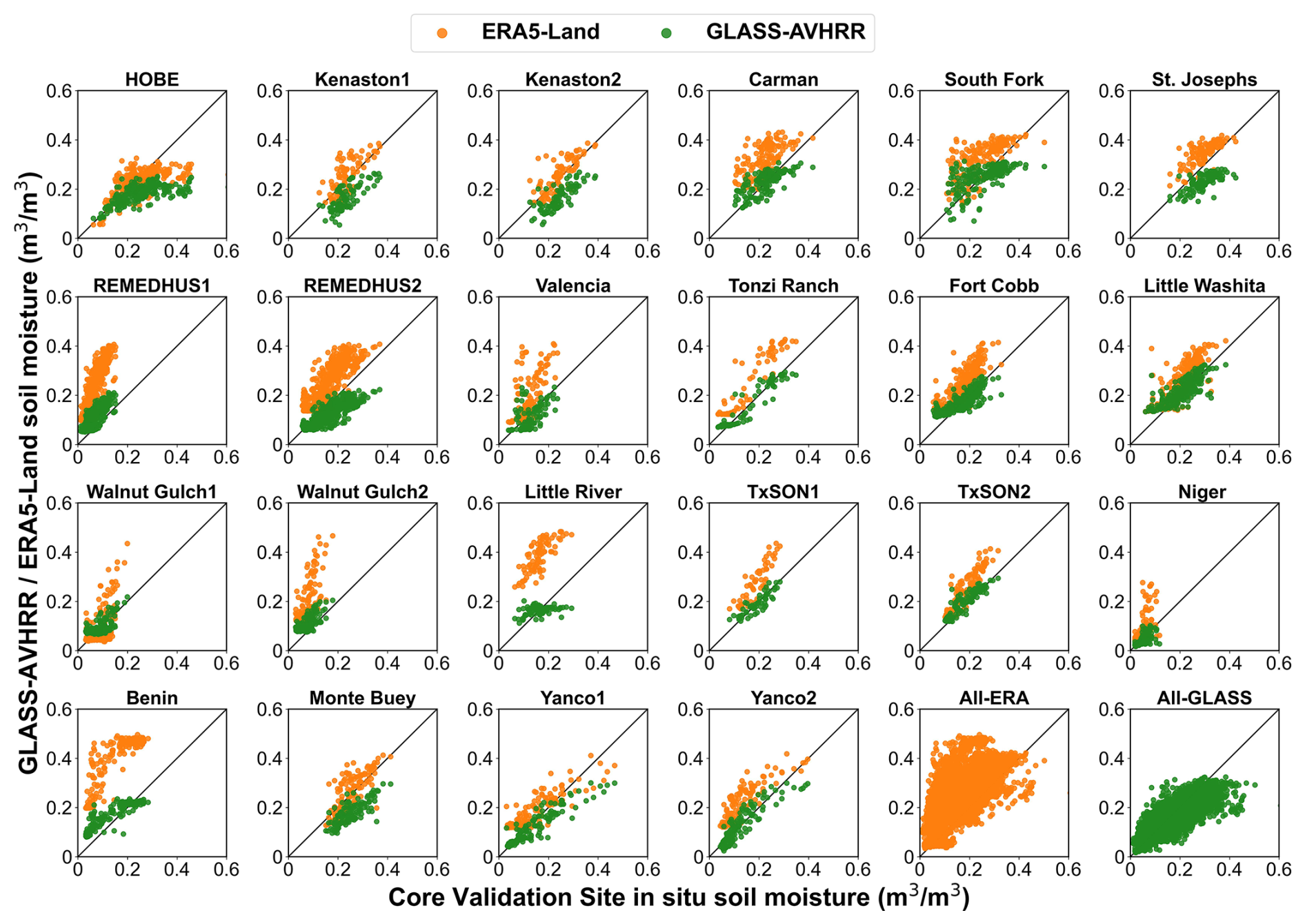
Figure 8 Scatter plots between the upscaled in situ SM and the corresponding estimated SM from the GLASS-AVHRR or ERA5-Land product at each SMAP core validation site.

To intuitively examine the ability of the GLASS-AVHRR SM product to capture temporal variations in measured SM and its temporal consistency with the GLASS-MODIS product, time-series curves for the GLASS-AVHRR (aggregated at 10 km), GLASS-MODIS (aggregated at 9 km), and in situ SM (upscaled at 9 km) at six CVSs with different land cover types were plotted, with the ERA5-Land SM product (∼9 km horizontal resolution) also included for reference (Fig. 9). Through extending the GLASS-MODIS SM product from 2000 back to 1982, the GLASS-AVHRR SM product attained complete temporal coverage from 1982 to 2021, and a high degree of temporal consistency between these two products could be observed from the time-series plots. Despite the fact that the ERA5-Land SM product also had long-term temporal coverage, it exhibited large wet biases when compared with the upscaled in situ SM at all six CVSs, whereas both the GLASS-MODIS and GLASS-AVHRR SM products aligned more closely with the dynamic ranges of measured SM. As mentioned above, the GLASS-AVHRR SM product exhibited notable dry biases at a few CVSs. However, as can be seen from the time-series curves at REMEDHUS2 (Fig. 9a) and Yanco1 (Fig. 9f), suspicious abrupt rises in measured SM, as well as temporary spikes in SM (possibly caused by irrigation), might also have partially contributed to these dry biases. Overall, the GLASS-AVHRR SM product could well capture the temporal variations in measured SM at these CVSs, except for the Little River site (Fig. 9d), where the land cover type is “Cropland or Natural mosaic”. Measured SM at this site did not show a clear seasonal pattern as at the other sites, and there was less consistency between the two GLASS SM products, likely due to the stronger spatial heterogeneity of this site. In addition, at the Walnut Gulch1 site (Fig. 9c), where the dominant land cover type is “Shrublands”, while the GLASS-AVHRR product captured high SM values well, it slightly overestimated when the measured SM approached zero.

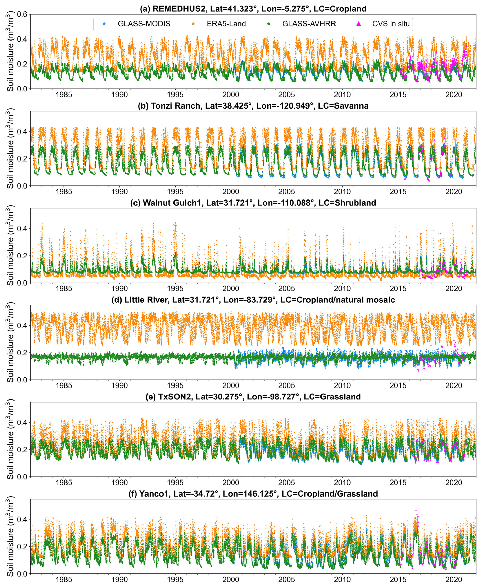
Figure 9 Time-series plots of the GLASS-AVHRR (aggregated at 10 km), GLASS-MODIS (aggregated at 9 km), ERA5-Land (∼9 km horizontal resolution), and in situ SM (upscaled at 9 km) at six CVSs with different land cover types for the period 1982–2021.

4.3 Spatial consistency with global SM products

To further investigate the spatial consistency between the GLASS-AVHRR and GLASS-MODIS SM products, as well as with two widely used long-term global SM products, mean SM maps of the GLASS-AVHRR, GLASS-MODIS, ESA CCI, and ERA5-Land products were plotted for January and July of 2016 (Fig. 10). It can be seen that the GLASS-AVHRR SM product had the most complete spatial coverage among these products, after masking out permanent snow and ice and water bodies (Fig. 10g and h). Despite the spatiotemporal continuity of the ERA5-Land reanalysis SM product, it yielded negative SM values close to 0 in parts of northern Africa, especially in July, which were masked out here (Fig. 10c and d). The ESA CCI combined SM product exhibited substantial spatial gaps above 30° N in January, in addition to the persistent absence of valid estimates in some densely vegetated regions (e.g., the Congo River and Amazon River basins), due to the attenuation of microwave signals in these areas (Fig. 10a and b) (Dorigo et al., 2017). Meanwhile, because of the lack of GLASS-MODIS albedo products at high latitudes during the cold season, GLASS-MODIS SM estimates were unavailable at high latitudes (above 60° N) in January (Fig. 10e). Nevertheless, this does not affect the complete spatial coverage of the GLASS-AVHRR SM product, although it should still be used with caution in areas covered by seasonal snow and ice. In this regard, the performance of the GLASS-AVHRR SM product during the winter season (December–February) was evaluated using ISMN stations located above 30° N latitude, retaining only those with more than 100 matched records. The product achieved a median R value of 0.69 at 374 representative ISMN stations during Period I (2000–2018) and 0.63 at 19 stations during Period II (1982–1999). Therefore, despite its relatively lower accuracy in winter, the GLASS-AVHRR SM product still can provide valuable estimates and serve as a useful complement to the ESA CCI SM product.

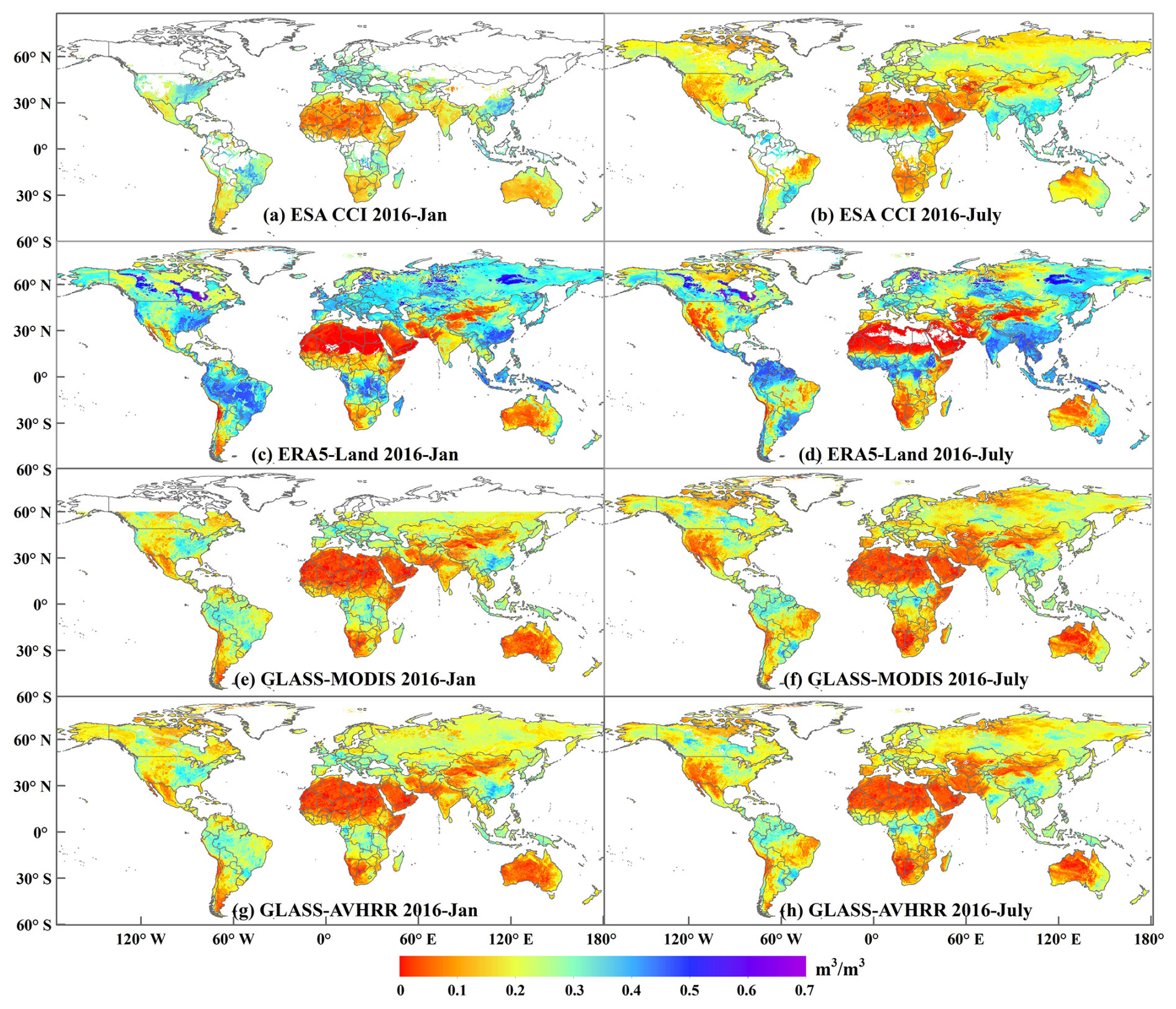
Figure 10 Mean global SM maps of the (a, b) 0.25° ESA CCI combined, (c, d) 0.1° ERA5-Land, (e, f) 1 km GLASS-MODIS, and (g, h) 5 km GLASS-AVHRR SM product in January and July of 2016. Permanent snow and ice as well as water bodies have been masked out using the MODIS land cover product (MCD12C1), while SM values at northern high latitudes in January should be interpreted with caution due to the widespread presence of permafrost, snow, and ice.

In terms of the spatial distribution patterns of SM, the GLASS-AVHRR and GLASS-MODIS SM products showed a high degree of consistency, which further demonstrates the effectiveness of the developed DL model. In general, both GLASS SM products were slightly drier than the ESA CCI combined SM product, probably because optical and thermal satellite SM estimates typically represent a shallower depth compared to microwave SM products. In contrast, the ERA5-Land SM product was much wetter than the other three SM products, especially in regions with high SM levels. While the three satellite SM products generally ranged between 0 and 0.5 m³ m⁻³, the ERA5-Land reanalysis SM product showed a range of 0–0.7 m³ m⁻³, indicating a clear tendency for overestimation. Although varying degrees of biases existed among the four global SM products, similar spatial patterns could be observed in all of them, characterized by higher SM values in the eastern United States, northern South America, central Africa, and southern Asia and lower SM values in the western United States, the Middle East, northern and southern Africa, and Australia. Moreover, July was slightly drier than January for all four SM products, particularly in regions such as the western United States, eastern South America, and central Asia.

Figure 11 presents a zoomed-in comparison between the four SM products across the Tibetan Plateau in July 2016. The Tibetan Plateau, located in central Asia, is the highest and most extensive plateau in the world, with an average elevation exceeding 4000 m. Its climate is extreme and varied, featuring significant seasonal and interannual variations. The unique topographic and climatic characteristics of the Tibetan Plateau make it one of the hotspots for global climate change research. As can be observed from Fig. 11, all of the SM products show similar spatial distribution patterns: lower SM levels in the western and northern parts of the plateau, where rainfall is scarce and vegetation is sparse, and higher SM levels in the eastern and southern regions, where rainfall is more abundant and vegetation is denser. The GLASS-AVHRR SM product also exhibited high spatial consistency with the GLASS-MODIS SM product over the Tibetan Plateau, indicating that the adopted DL model effectively learned spatial features from the target SM product without introducing significant biases. Compared to the other three products, the ERA5-land SM product was much wetter in the southern part of the plateau, and the large positive bias in the ERA5-land reanalysis SM over the Tibetan Plateau was also reported in a previous study (Xing et al., 2021). Notably, there were many small patches with abrupt SM changes in the ERA5-land product (Fig. 11c), which were markedly improved in both the GLASS-AVHRR and GLASS-MODIS SM products. Moreover, compared to the ERA5-land and ESA CCI SM products at coarser resolutions, the GLASS-AVHRR SM product contained much richer spatial details and could well capture the distribution patterns of topography and vegetation.

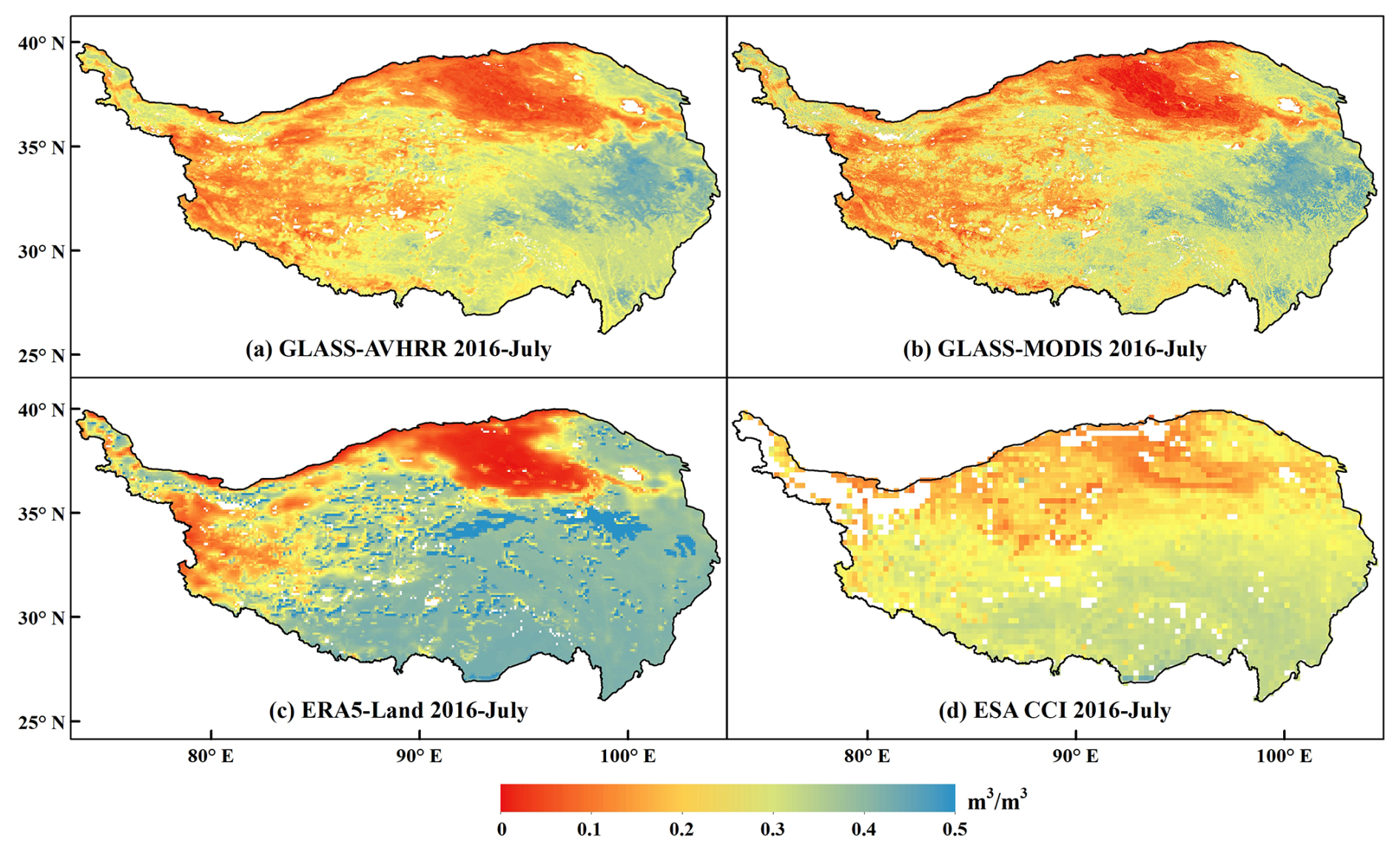
Figure 11 Zoomed-in comparison of the (a) 5 km GLASS-AVHRR, (b) 1 km GLASS-MODIS, (c) 0.1° ERA5-Land, and (d) 0.25° ESA CCI combined SM products across the Tibetan Plateau in July 2016. Permanent snow and ice as well as water bodies have been masked out using the MODIS land cover product (MCD12C1).

5 Discussion

This study aimed to develop a long-term global SM estimation framework using DL models to derive a temporally consistent SM product with reliable accuracy over the last four decades. Therefore, we mainly explored two types of widely used DL models that are adept at processing sequential data: the LSTM-based models and transformer. While LSTM has been utilized to retrieve SM since 2017 (Fang et al., 2017), the state-of-the-art transformer model is still rarely used for SM estimation. Specifically, the accuracy of these DL models was compared from multiple perspectives, such as comparisons between the DL models and the benchmark tree-based XGBoost model, between models with different attention mechanisms, or between models with different application architectures. The results showed that the attention-based LSTM (AtLSTM) model achieved the best performance on the test set and that the MTM architecture could output a sequence of SM estimates simultaneously while maintaining similar accuracy to that of the MTO architecture. Note that transformer was reported to outperform the LSTM-based models in several hydrological applications due to its ability to better handle long sequences and relate any two positions in the sequence (Amanambu et al., 2022; Yin et al., 2022). Meanwhile, according to Xu et al. (2021), transformer achieved similar accuracy to the AtLSTM model in multi-temporal crop mapping tasks. However, Zeng et al. (2023) found that a simple linear model can outperform transformer in long-term time-series forecasting tasks and ascribed this to the temporal information loss associated with the self-attention mechanism. Therefore, the superiority of transformer for time-series forecasting or estimating remains a topic of ongoing debate (Amanambu et al., 2022; Xu et al., 2021; Yin et al., 2022; Zeng et al., 2023). In our study, the accuracy of the transformer model was slightly lower than that of the AtLSTM model, particularly for samples with high SM levels ($>\mathrm{0.4}{\mathrm{m}}^{\mathrm{3}}{\mathrm{m}}^{-\mathrm{3}}$). Given the high temporal variability of SM and the relatively short temporal length of SM memory, which typically ranges from 5 to 40 d and diminishes with increasing time lags (Orth and Seneviratne, 2012), this result may be attributed to the superior ability of the AtLSTM model to capture short-term adjacent dependencies. Yet, additional experiments with diverse training datasets are necessary to confirm the general applicability of this result.

We also investigated the effect of input sequence length on model accuracy, and it was found that the overall accuracy of the AtLSTM model with the MTM architecture leveled off at a sequence length of about 4 d. Subsequent analysis of the distribution of attention weights indicated that the model could automatically learn the necessary temporal information from adjacent positions in the sequence to accurately estimate SM. Despite the fact that the overall accuracy of the LSTM-based models with the MTM architecture would converge as long as the length of the input sequence is sufficiently long, the models' accuracy is typically lower at the beginning or end of the sequence, and the affected estimates need to be identified and removed. In contrast, most of the current LSTM or transformer application architecture is MTO, and the accuracy remains unaffected at both ends of the sequence. However, it is still necessary to identify the optimal sequence length during the training process to improve model efficiency, as the amount of input data would increase substantially with increasing sequence length. Here, we mainly explored the ability of the LSTM-based models and transformer to capture temporal information from time-series input datasets for SM estimation. Future research could consider incorporating spatial patterns by combining the AtLSTM or transformer models with CNNs or adapting the network of transformer to improve its applicability for time-series estimating tasks. Moreover, different input features and data sources can be integrated to investigate whether the estimation accuracy of SM can be further improved.

To examine the accuracy and consistency of the generated four-decade global daily GLASS-AVHRR SM product, different strategies were combined to fully evaluate it, including the validation against in situ SM datasets from point-scale ISMN stations, field-scale COSMOS networks, and upscaled 9 km SMAP CVSs, separately, as well as the intercomparison with two widely used long-term global SM products. However, the evaluation of the GLASS-AVHRR SM product is still subject to certain limitations. The ISMN in situ SM dataset prior to 2000 is relatively scarce, with only 45 independent stations available for evaluation during this period, and a large-scale difference exists between this point-scale SM dataset and the 5 km GLASS-AVHRR SM product. The COSMOS sensors generally have varying footprint radii and sensing depths, and their measurements tend to exhibit higher uncertainties in organic soils or humid regions, which can lead to spatial and vertical representativeness issues. Additionally, there is only a limited number of upscaled SMAP CVSs, and the data collected may also contain errors caused by varying degrees of spatial representativeness.

Although the validation results demonstrated that the GLASS-AVHRR SM product achieved high accuracy across different spatial scales, its performance was inevitably influenced by the GLASS-MODIS SM product, which served as the training target for the SM estimation model. Meanwhile, as a data-driven product, the quality of the GLASS-AVHRR SM product largely depends on the selected input features, their accuracy and consistency, and the representativeness of the training data. Potential uncertainties may arise from biases or errors in the satellite and reanalysis inputs. In particular, the reduced model accuracy observed in the high SM range is likely due to the inherent imbalance in the numerical distribution of SM samples and increased uncertainty in the accuracy of input features under wet surface conditions. In terms of feature selection, due to constraints such as record length, spatiotemporal completeness, and accuracy requirements, some informative but less consistently available variables may have been excluded, further contributing to the uncertainties in the final SM product. Moreover, as the ERA5-Land reanalysis SM was used as one of the input features, the generated product cannot be considered entirely independent. Future research could explore developing a fully independent, long-term, and seamless global SM product with sufficiently reliable accuracy.

Nevertheless, intercomparison with the long-term ERA5-Land and ESA CCI combined SM products showed that the derived GLASS-AVHRR SM product achieved the most complete spatial coverage, contained much richer spatial details, and remained unaffected by the large wet biases present in the input ERA5-Land SM product. While cumulative distribution function (CDF)-based methods can also be used for bias correction, they typically adjust statistical distributions locally, which limits their spatial generalization capability, particularly in regions lacking in situ SM data. In addition, they often overlook the temporal dependencies and non-linear dynamics inherent in SM time series. Therefore, both the proposed DL-based SM estimation framework and the derived long-term global SM product present clear value. It should be noted that the ESA CCI combined SM product was generated by synthesizing SM products retrieved from multiple microwave sensors using different algorithms. This approach was necessary because no single microwave sensor covered the sufficiently long time period (>30 years) required for a climate data record, but it also inevitably led to variations in the product's accuracy over time and space (Dorigo et al., 2012). In contrast, the GLASS-AVHRR SM product was estimated using mainly the seamless GLASS-AVHRR albedo and LST products retrieved from the long-archived AVHRR satellite observations spanning four decades, which ensured its spatial and temporal completeness and consistency. Moreover, although microwave sensors are more sensitive to SM, their signals are significantly attenuated in densely vegetated areas, resulting in persistent data gaps in the ESA CCI product. Although the GLASS-AVHRR SM product is less accurate in these regions (with a median R of 0.57 at 20 COSMOS forest stations), it can provide a valuable complement to microwave SM products. In future research, greater efforts should be devoted to both the development and validation of long-term SM climate data records, and it is also crucial to assess the long-term trends in these SM datasets.

6 Data availability

The seamless global 5 km SM product (GLASS-AVHRR SM) at daily scale from 1982 to 2021 is freely accessible at https://glass.hku.hk/archive/SM/AVHRR/ (last access: 18 September 2025). Additionally, the annual average GLASS-AVHRR SM dataset was generated, which can be downloaded from https://doi.org/10.5281/zenodo.14198201 (Zhang et al., 2024b). Note that this product represents the volumetric water content in the uppermost soil layer (0–5 cm), with areas of permanent snow and ice and water bodies masked. A scale factor of 1000 was applied, with missing values filled with −9999.

7 Conclusions

A four-decade (1982–2021) seamless global surface SM product (0–5 cm) at 5 km resolution was derived here, denoted as the GLASS-AVHRR SM product. This product was estimated using mainly the long-archived AVHRR satellite observations and multi-source datasets based on DL. Specifically, a large number of evenly distributed training samples extracted from the global 1 km daily GLASS-MODIS SM product were used as the target to train three LSTM-based models (LSTM, Bi-LSTM, and AtLSTM) and a transformer model, with an XGBoost model employed as the benchmark. After identifying the AtLSTM as the best-performing model, it was ultimately adopted to generate the long-term GLASS-AVHRR SM product, which was then fully evaluated for reliability and consistency. The main results are summarized as follows:

1. Evaluation of the models on the test set showed that all four DL models outperformed the benchmark XGBoost model, particularly at high SM levels ($>\mathrm{0.4}{\mathrm{m}}^{\mathrm{3}}{\mathrm{m}}^{-\mathrm{3}}$). Notably, the AtLSTM model achieved the best performance, with an R² of 0.987 and RMSE of 0.011 m³ m⁻³, and its SM estimates were much closer to the 1:1 line than those from the other models. These results indicate that utilizing bidirectional temporal information from the input sequence as well as adding an attention module are both effective in improving the accuracy in estimating SM. Meanwhile, The MTM architecture adopted in this study achieved similar accuracy to that of the MTO architecture while being able to output a sequence of SM estimates simultaneously and considerably reduce the production time.

2. The AtLSTM model with the MTM architecture was then employed to investigate the effect of input sequence length on model accuracy, and it was found that the overall accuracy of the model leveled off at a sequence length of about 4 d. Further analysis of the attention weights revealed that the AtLSTM model with the MTM architecture could automatically learn the necessary information from adjacent positions in the sequence to accurately estimate SM at each position. In contrast, the temporal information learned by the self-attention module of the transformer model was more dispersedly distributed, and the slightly lower accuracy of the transformer model than the AtLSTM model might be attributed to the typically high temporal variability of SM and the fact that short-term adjacent temporal information played a more critical role in the accurate estimation of SM.

3. The derived GLASS-AVHRR SM product was first evaluated using 45 independent point-scale ISMN stations prior to 2000, resulting in a median R of 0.73 and ubRMSE of 0.041 m³ m⁻³. Then, the product was validated against SM datasets from three post-2000 field-scale COSMOS networks, with median R values ranging from 0.63 to 0.79 and median ubRMSE values between 0.044 and 0.065 m³ m⁻³. Validation of the GLASS-AVHRR SM product at 22 upscaled 9 km SMAP CVSs yielded an overall R of 0.82 and ubRMSE of 0.054 m³ m⁻³. Whereas the ERA5-Land SM product had large wet biases at most of the CVSs, the GLASS-AVHRR SM product basically corrected these biases. Moreover, the time-series plots at six CVSs further demonstrated that the GLASS-AVHRR SM product could well capture the temporal variations in measured SM and showed a high degree of temporal consistency with the GLASS-MODIS SM product.

4. Finally, the GLASS-AVHRR SM product was intercompared with two widely used long-term global SM products to investigate their spatial consistency. With the most complete spatial coverage, the GLASS-AVHRR SM product was slightly drier than the ESA CCI combined SM product, possibly due to the shallower depth it represents, whereas the ERA5-Land SM product exhibited a clear tendency for overestimation. Although similar spatial patterns of SM could be observed in all of these products, the GLASS-AVHRR SM product contained much richer spatial details than the two long-term SM products at coarser resolutions.

Our study demonstrates the feasibility of utilizing the attention-based DL model and AVHRR satellite observations to generate a long-term global SM product. The derived GLASS-AVHRR SM product has the advantages of long-term coverage, spatial and temporal integrity, reliable accuracy, and consistency. As a reliable extension of the GLASS-MODIS SM product and a valuable complement to microwave SM products, this four-decade global SM product will be beneficial for a range of large-scale climate-change-related research. Future studies could combine other DL models or integrate different data sources to further improve the quality of the long-term SM product.

Appendix A: Supplementary figures

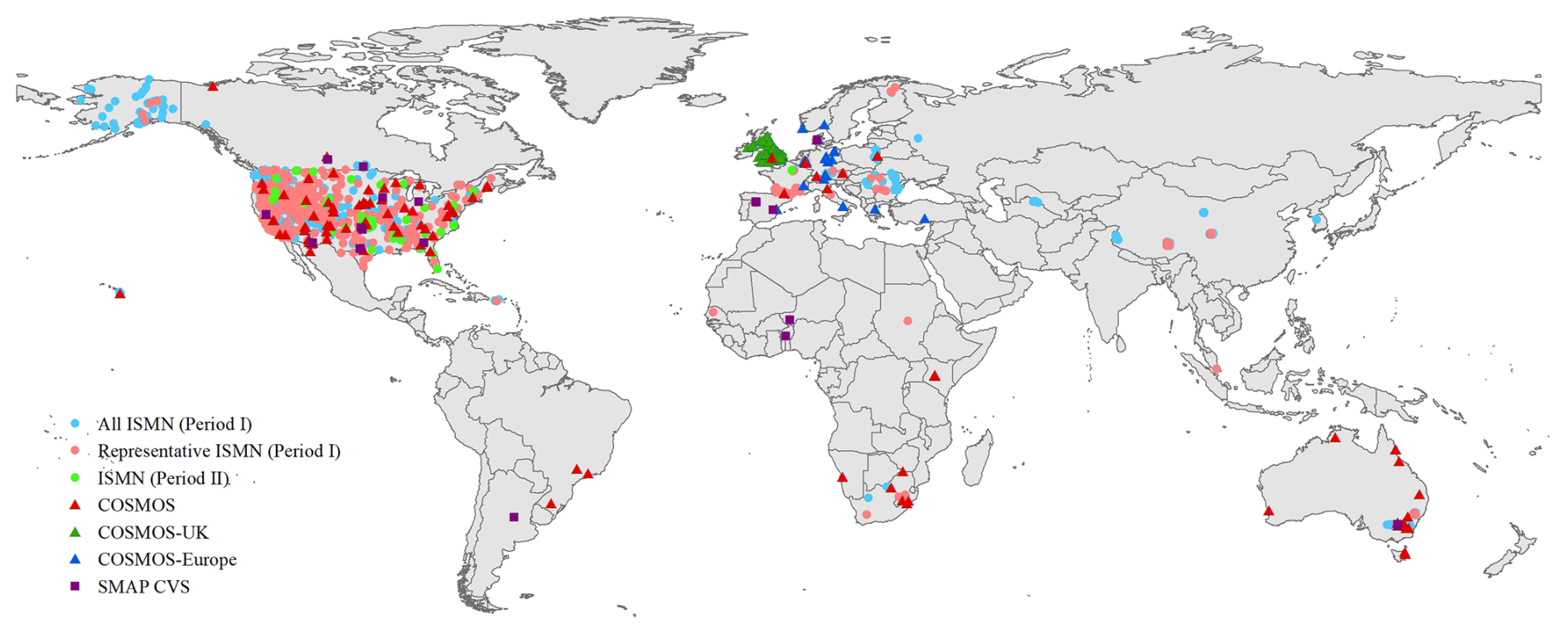
Figure A1 The spatial distribution of SM stations for each in situ SM dataset used in this study. Period I refers to 2000–2018, and Period II refers to 1982–1999.

Figure A2 Boxplots of sensing depths across the three COSMOS networks used for validation.

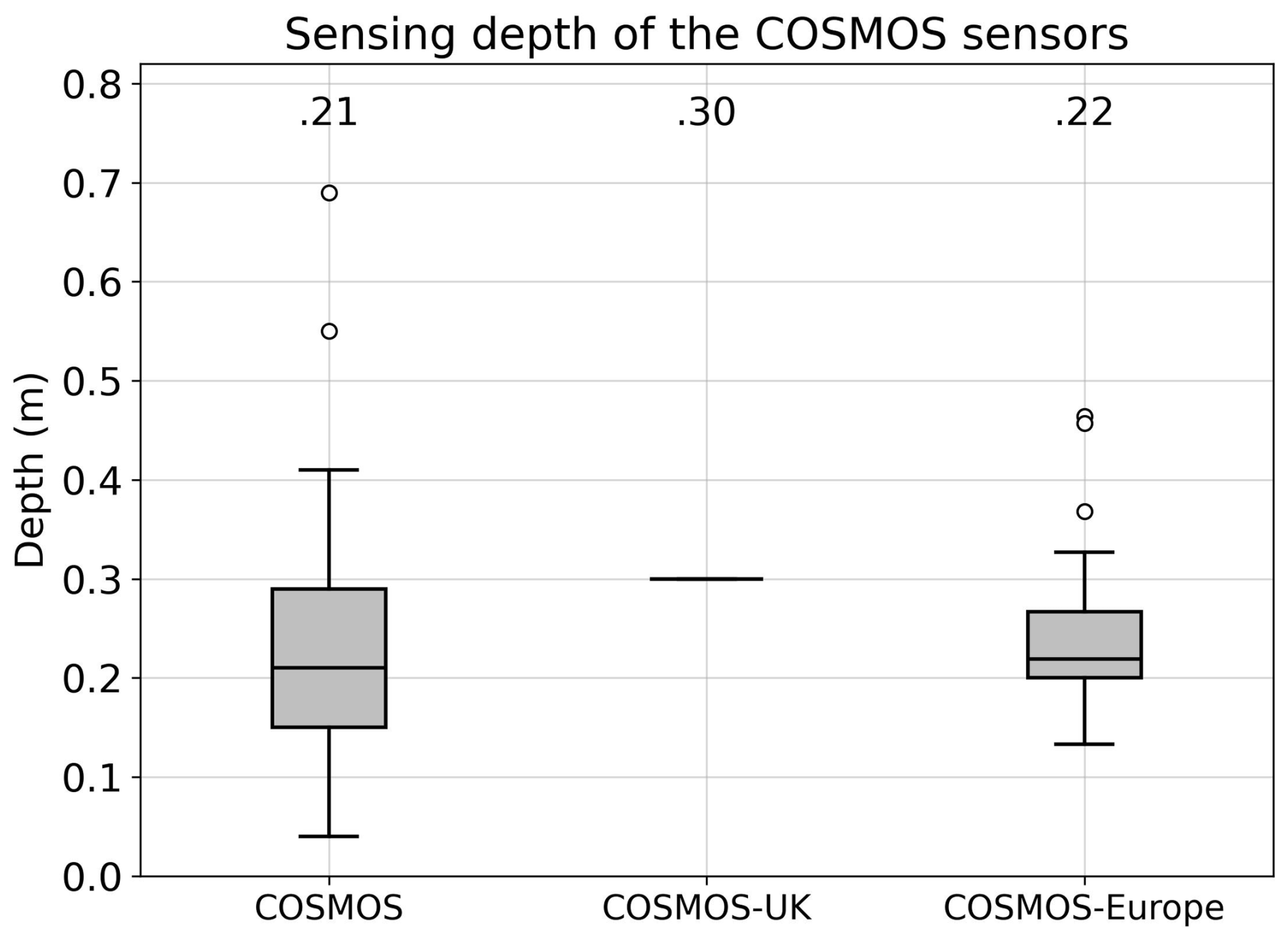
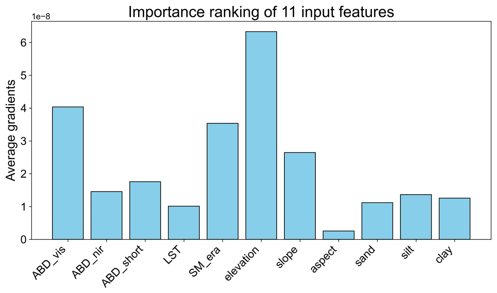
Figure A3 Importance ranking of 11 input features for the At-LSTM model based on gradient analysis.