Global-PCG-10: a 10 m global map of plastic-covered greenhouses derived from Sentinel-2 in 2020

Plastic-covered greenhouse (PCG) is widely used in agricultural production due to its temperature control, water conservation, and wind protection characteristics, significantly enhancing crop yields and economic benefits. However, its long-term and extensive use can lead to environmental issues, such as the accumulation of local toxic gases and the degradation of soil physicochemical properties. Therefore, obtaining a comprehensive distribution of PCGs is essential. To monitor PCGs on a large scale, this study developed a novel approach for producing the first global 10 m PCG dataset (Global-PCG-10) with high-quality. Firstly, the globe was divided into multiple 5° grids, and grids for classification were organized based on global cropland layer. Then, multi-temporal Sentinel-2 data and initial labels of PCGs were obtained through Google Earth Engine (GEE) to create a training set for deep learning. Next, initial labels were optimized with the active learning strategy combined with the deep learning model, APC-Net. Finally, the PCG classification results were predicted, spatially analyzed, and compared with publicly released land use and land cover (LULC) datasets. Experimental results indicate that the proposed Global-PCG-10 dataset (Niu et al., 2024) has a high overall accuracy of 98.04 % ± 0.12 %. The global area of PCGs is 14 259.85 km², and 69.24 % of PCGs are located in Asia, covering around 9874.51 km². China has the largest PCG area of 8224.90 km², accounting for 57.67 % of the globe and 83.29 % of Asia. Comparisons with other LULC datasets revealed that PCGs, which should be classified as cropland, are often misclassified as bareland, impervious surfaces, ice/snow, etc.

1 Introduction

With the rapid development of modern plastic industry, agricultural plastic-covered greenhouses (PCGs) have been spreading widely around the globe. According to statistics, the total PCG area of the world has reached to 1.3 million ha (Tong et al., 2024), accounting for 8 ‰ of the global cropland (global cropland data source from: https://www.fao.org/faostat/en/#data/RL, last access: 23 September 2025). One important reason for the widespread of PCGs is the role in the increase of both crop yield and quality. Local climatic conditions could be greatly improved for crops with an increased accumulated temperature and a decreased water evapotranspiration, which is significant especially for regions with adverse climatic situations (Liu and Xin, 2023; Lu et al., 2018). In addition, the globe witnesses a speedy growth of PCGs recently. Countries that have a large area of PCGs mainly include China, Spain, Italy, Vietnam, etc. (Feng et al., 2022a; Jiménez-Lao et al., 2020; Veettil et al., 2023; Wu et al., 2016).

Although PCGs play a key role in modern agriculture for the improvement of crop yield and quality, the demerits of PCGs could not be neglected. Firstly, PCGs increase both the cropping and land use intensity. Due to the improvement of hydrothermal conditions, the crops could now be harvested twice or three times within one year, leading to the overexploitation of soil nutrients and underground water resources. Along with the cropping intensity, the usage of chemical fertilizers and pesticides has also been increased, which would lead to the widespread of soil contamination. Therefore, the existence of PCGs could be viewed as an important indicator of agricultural non-point source pollution. Secondly, PCGs have changed the pattern of water evapotranspiration, which hinders the circulation of water and may cause the microclimate anomaly. Finally, PCGs contribute more greenhouse gas emissions than other farmlands (Niu et al., 2023b; Wang et al., 2022).

Therefore, it is of great significance to acquire the accurate spatial distribution of PCGs worldwide to understand where and how much PCGs are located and constructed globally. Due to the large-scale coverage and cost-effectiveness, Earth Observation technology especially satellite remote sensing has been widely used for PCG classification. Commonly used satellites consist of Landsat-5/7/8, IKONOS, QuickBird, WorldView-1/2/3 and ESA's Sentinel-2, which all belong to multispectral satellites (Hao et al., 2019; Ou and Wang, 2022). In addition to the aforementioned multispectral data, some researchers have used free RGB remote sensing imagery from Google Earth for PCG classification (Niu et al., 2023a; Zhang et al., 2021b). There are three main kinds of classification methods used for PCG mapping: spectral based methods, machine learning based methods, and deep learning-based methods.

Spectral based methods tried to construct a spectral index which is sensitive to plastic greenhouses. The differences of PCGs and the background could be enlarged by these spectral indexes, where a threshold is used to extract PCGs (Aguilar et al., 2022; Zhao et al., 2004). The merit of spectral index is the unnecessary for training samples, while the demerit is the uncertainty in obtaining the suitable threshold in large-scale regions. This is because the best threshold for PCG extraction may be different in different regions, which is influenced by the spectral variations of both PCGs and the background (González-Yebra et al., 2018; Lu et al., 2014). Aguilar et al. (2016) and Yang et al. (2017) independently developed greenhouse indices, the Moment Distance Index (MDI) and the Plastic Greenhouse Index (PGI), using Landsat satellite data. Similarly, Zhang et al. (2022a) derived the Advanced Plastic Greenhouse Index (APGI) from Sentinel-2 imagery through band calculations.

In terms of machine learning based methods, decision tree, support vector machine (SVM) and random forest (RF) are commonly used supervised classifiers for PCG mapping. Compared with spectral index, the merit of machine learning is its robustness. However, its drawback is the reliance on labeled samples, where the quantity, quality and diversity of these samples significantly affect classification performance (Qiu et al., 2022, 2024; Zhang et al., 2024a). Additionally, “salt-and-pepper effect” is unneglectable in machine learning classifications (Du et al., 2022). Recently, Google Earth Engine (GEE) provides a popular remote sensing cloud platform, which integrates the aforementioned machine learning methods and provides vast volume of multi-source, multi-temporal remote sensing data, along with powerful cloud computing service (Feng et al., 2024; Li et al., 2023; Zhang et al., 2022c). This significantly enhances efficiency in large-scale mapping applications such as global LULC mapping, global wetland mapping, etc. Zhang et al. (2020, 2021a, 2022b, 2024c, d) used GEE to develop a comprehensive technical workflow for generating multiple global land cover data products, including a global impervious surface dataset, a global 30 m LULC dataset, etc. With regard to PCG classification, Ou et al. (2021) generated a 30-year PCG distribution map in Shandong Province, China, using Landsat series satellite data and the RF classifier on the GEE cloud platform. Similarly, by utilizing multi-year Landsat series satellite data and RF classifier on GEE, Gao et al. (2022) produced a 20-year greenhouse distribution map for the Guanzhong Plain area in Shaanxi Province, China. Besides, in our previous study, we utilized RF together with a partition modeling strategy to generate the first publicly released 30 m national PCG map of China with an overall accuracy of 87 % (Feng et al., 2021). Furthermore, we also tackled the long-neglected issue of the confusion between PCGs and plastic-mulched farmlands (PMFs) by introducing multi-temporal observations (i.e., film-on and film-off) to exclude PMFs from PCGs (Feng et al., 2022b).

In recent years, deep learning has achieved remarkable success in the fields of computer vision (CV) and natural language processing (NLP). Unlike classical machine learning methods, which can only capture the shallow features of input data, deep learning has a deeper neural network structure and can effectively learn images' semantic features, leading to a better robustness and generalization ability (Chen et al., 2022; Niu et al., 2022; Zhang et al., 2023). However, the performance of deep learning models heavily depends on the quantity and quality of training samples, which calls for a huge workload for sample labeling. The deep learning model has also been applied to PCG and PMF classification. For instance Zhou et al. (2024) developed a general framework for extracting PCGs, integrating prior knowledge with deep learning models. Li et al. (2022), Liu et al. (2023), and Chen et al. (2021) employed Google Earth imagery as their data source, selecting specific regions within Shandong of China or other smaller areas as study sites, and built deep learning models for PCG extraction. Additionally, Ma et al. (2021) and Chen et al. (2023) applied high-resolution remote sensing imagery (1 m resolution) and an object detection model to extract PCGs across China, however, these datasets have not been released publicly. In our previous study, we have proposed a dilated and non-local convolutional neural network (DNCNN) for the accurate delineation of PCGs in several key regions from China, Saudi Arabia, Turkey and Spain and achieved a high OA of about 90 % (Feng et al., 2021; Niu et al., 2023a). In May 2024, the University of Copenhagen released the first publicly accessible global dataset for large-scale PCG mapping (Tong et al., 2024), which was derived from PlanetScope commercial satellite imagery with a spatial resolution of 3 m and a deep learning model, UNet. While the dataset demonstrates good precision and coverage, acquiring such high-resolution, globally covered commercial satellite data remains prohibitively expensive for most researchers. Therefore, how to use open access satellite data such as Sentinel-2 and Landsat to generate a global PCG map still remains a challenging task.

To address this issue, this study utilizes Sentinel-2 satellite image, one of the most influential open-source remote sensing datasets globally, for PCG extraction. The temporal consistency and continuous, all-weather Earth observation capabilities of Sentinel-2 data effectively mitigate the temporal inconsistency found in commercial high-resolution datasets. Meanwhile, Sentinel-2 offers the highest resolution open-source remote sensing data, making it well-suited for PCG classification tasks. With such high data quality that is widely preferred by researchers, many existing data products are derived from Sentinel-2, allowing our Global-PCG-10 dataset to integrate with these data products seamlessly. For data organization, we have designed a global grid system to facilitate PCG data indexing and accessibility for researchers. However, Sentinel-2 satellite image is not perfect. Unlike high-resolution data, the 10 m resolution Sentinel-2 data contains a significant number of mixed pixels, which poses challenges for accurate extraction of PCGs. To address this issue, we utilize multi-temporal Sentinel-2 data to enhance the differentiation between PCGs and other confused land covers such as PMFs and bareland. Moreover, we have designed a framework that integrates active learning into deep learning model, improving the robustness of the latter when dealing with large-scale PCG mapping tasks.

Overall, we proposed a novel framework to generate the firstly publicly released 10 m global PCG map in 2020 derived from Sentinel-2. We also analyzed the spatial pattern of PCGs around the globe together with the driving force behind. Furthermore, we validated the accuracy of Global-PCG-10 and compared with other studies to further show its merits and demerits.

2 Dataset

2.1 Cropland layer

It should be noted that almost all of the PCGs lie in the cropland, where other land covers such as forest, water bodies and grassland witness no PCGs. Therefore, we resort to the global cropland layer to eliminate the classification errors (i.e., mainly false positives) in the regions that have a very low probability of PCGs. Nonetheless, there still might be PCGs that lie outside of the cropland layer. To tackle this issue, firstly, we divided the globe into a total of 2592 grids with a size of 5°×5° in the WGS84 projection, while retaining those grids that contained cropland cover. These retained grids extend, which is larger than the initial cropland, were designated as the first-level classification unit for data organization (i.e., blue grids in Fig. 1). Each 5°×5° grid was further divided into 25 grids of 1°×1°, which served as the second-level classification unit. Ultimately, we retained the grids that contained PCG predictions in the second-level classification units (i.e., orange grids in Fig. 1). In specific, we compared a series of open-access global LULC maps and selected GLC_FCS30D (Zhang et al., 2024c) as cropland layer due to its good performance.

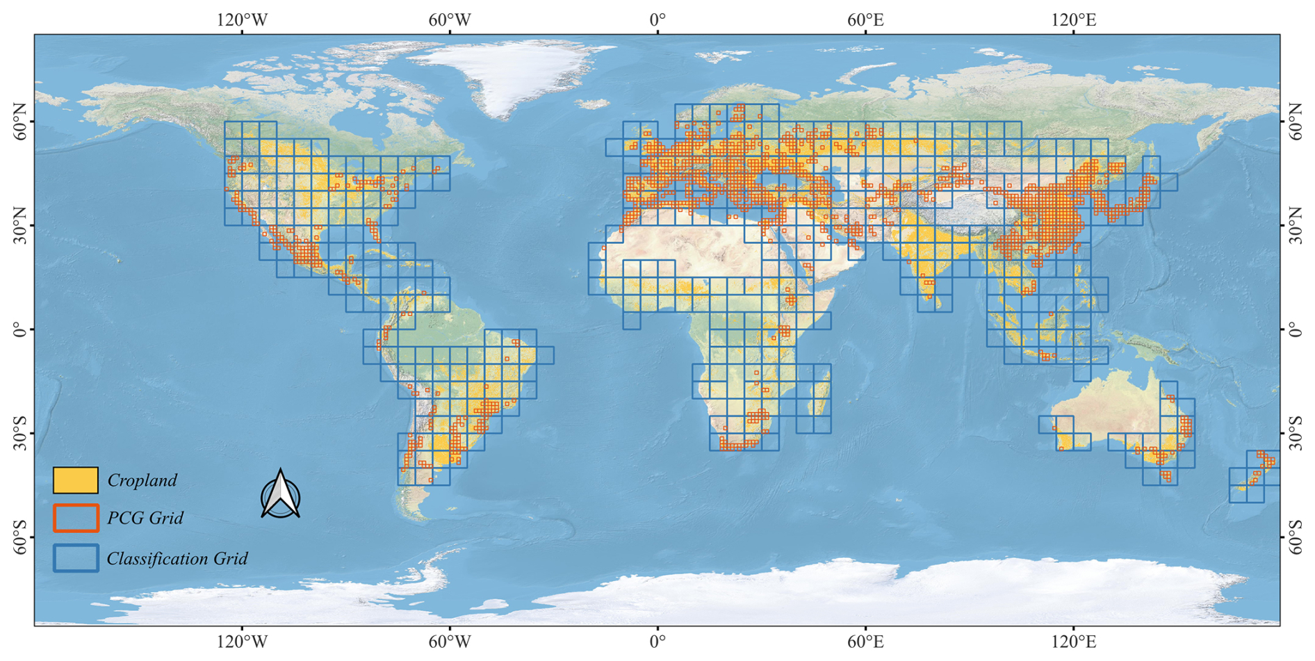
Figure 1 Spatial distribution of Cropland, PCG grid and classification grid. (Note: the yellow pixels indicate the cropland layer, which sources from the GLC_FCS30D cropland category (Zhang et al., 2024c), the orange grids stand for 1° grids that contain PCG classification results, and the blue grids represent the original 5° grids used for PCG classification.)

2.2 Satellite datasets

Sentinel-2 multispectral images were used in this study. As the important part of ESA's Copernicus Programme, Sentinel-2 aims to provide global Earth Observation data at a fine scale with 10 m captured by MultiSpectral Instrument (MSI) with a total of 13 bands and a swath width of 290 km. Sentinel-2 is a satellite constellation initially composed of Sentinel-2A and Sentinel-2B, which operate in the same sun-synchronous orbit but are phased 180° apart to ensure a high revisit frequency. In addition, Sentinel-2C, the third satellite in the constellation, was successfully launched in March 2024. It serves as a replacement unit to ensure data continuity and system redundancy throughout the mission duration. Several reg-edge bands that are very sensitive to vegetation have been designed in Sentinel-2, which could capture a more detailed conditions of vegetated regions than other satellites such as Landsat and MODIS.

In addition, Sentinel-2 has two major merits over Landsat for PCG mapping around the globe. Firstly, Sentinel-2 has a finer spatial resolution of 10 m. When compared with Landsat data at 30 m resolution, PCGs on Sentinel-2 images show a rather neat and tidy boundaries. Besides, Sentinel-2 witness much less mixed pixels than Landsat due to the increase of spatial resolution. Secondly, the revisit time of Sentinel-2 is 5 d at the equator while 2–3 d at mid-latitudes, which is much shorter than the 16 d of Landsat. The frequent revisit of Sentinel-2 is very important for large-scale PCG mapping performance, since it increases the possibility to composite could-free images, especially for those cloudy and rainy regions around the world.

3 Method

Figure 2 depicts the overall workflow of this study, which consists of three stages.

1. Stage-1: generating initial PCG labels via random forest classifier and the GEE cloud platform, which aims to release human labor in PCG label annotation;

2. Stage-2: producing accurate PCG classification results through a deep learning model combined with an active learning strategy, which adopts a coarse-to-fine procedure to generate high-quality PCG maps;

3. Stage-3: finalizing global PCG mapping and conducting spatial analysis.

Figure 2 Schematic flowchart to produce the Global-PCG-10 dataset.

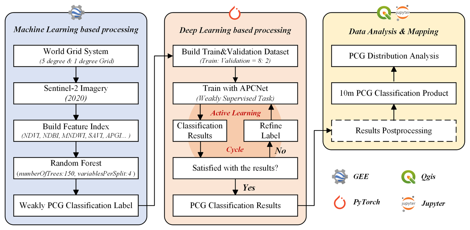
Specifically, firstly, both PCG and non-PCG samples were labeled on GEE platform in the format of point. The locations of samples were acquired from both visual inspection on very high resolution images on Google Earth and our previous field survey records. Multi-temporal and cloudless Sentinel-2 images in 2020 were composited by GEE, from which a multi-dimensional feature space for PCG classification was constructed, including spectral indices (i.e., NDVI, MNDWI, etc.), texture features and recently published plastic greenhouse indexes (i.e., APGI, PGHI, etc.). The RF classifier was then used to generate initial labels. Afterwards, the label dataset was split into training and validation sets in 8:2, and the APC-Net model was built using the PyTorch framework. The initial and weak labels were refined through the active learning strategy with the APC-Net model, continuously improving the PCG classification performance. Finally, post-processing was applied to the PCG classification results to eliminate isolated noises and then followed by spatial analysis and mapping.

3.1 Stage-1: PCG weak label generation

In the field of large-scale remote sensing classification, the quantity and quality of labels are very important. However, if using only human annotation, it would be time-consuming to acquire enough samples for global PCG classification. To tackle this issue, we first employed GEE and random forest to generation the initial PCG classification maps, from which samples (i.e., denoted as weak samples) are refined to train a deep semantic segmentation model.

The weakly labeled samples used in this study were generated through the RF classifier on GEE platform and sourced from regions with large amount of PCGs. And prior to training the deep learning model, we implemented multiple strategies to ensure the accuracy and reliability of initial PCG labels, as detailed below.

1. Collection of high-confidence samples: to construct the training samples required for GEE-based Random Forest (RF)classification, we conducted field surveys in key greenhouse-intensive regions in China (e.g., Weifang in Shandong, Kunming in Yunnan, and Lishu in Jilin). During the surveys, we also consulted local farmers to confirm the locations and types of PCG. Considering that PCG typically remain in use for around 10 years or more with relatively high stability (Ou et al., 2021), we performed systematic manual visual interpretation of historical high-resolution imagery from Google Earth in multiple global regions to obtain high-confidence samples. For areas outside China, we additionally referred to published literature, meta-analyses and online sources for auxiliary identification. All samples were further verified using Sentinel-2 imagery to ensure their actual presence in the year 2020. We also refined PCG and non-PCG labels based on the RF classification results within each grid to enhance overall labeling accuracy.

2. Quality assessment and selection of RF classification results: based on the collected samples, we trained a RF model with GEE, using a split between training and validation sets. A confusion matrix was constructed to evaluate the classification accuracy, where the validation set was excluded from the training process and used solely for accuracy assessment. Only those classification maps with an overall accuracy (OA) greater than 95 % and a user accuracy (UA) for the PCG class above 90 % were selected as candidate label maps for training the deep learning model.

3. Final screening of training labels for the deep learning model: all candidate label maps were undergone further visual inspection. Each 512×512 pixels image patch was visually checked to ensure high annotation quality, and only the regions with the most reliable classification results were retained for deep learning model training. This process ensured that the final training labels used in the deep learning model were of high reliability.

Figure 3 shows several examples from six typical regions, including Weifang, China (Asia); Almeria, Spain (Europe); Uruapan, Mexico (North America); Campinas, Argentina (South America); Agadir, Morocco (Africa); and Coffs, Australia (Oceania). However, the “salt-and-pepper effect” still exists in RF classification results in Fig. 3. This is also the reason why we introduce the second stage (i.e., deep learning and active learning) to refine PCG maps. Notably, misclassifications are in areas with highly reflective surfaces, such as factory rooftops, beaches, deserts, and bareland.

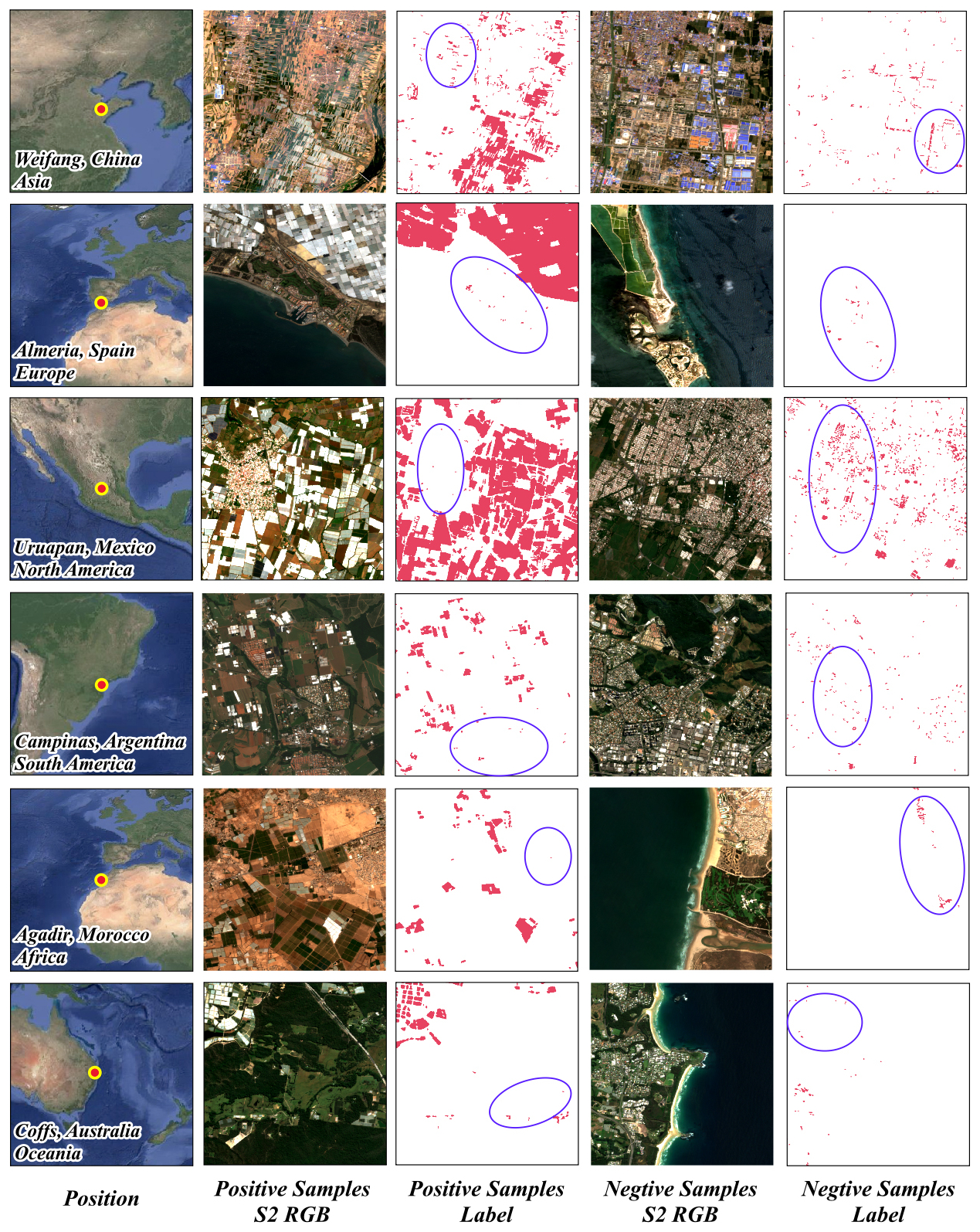
Figure 3 Reference samples and their position in the world. (Note: blue circle represents the “salt and pepper effect” in the reference samples. The size of the reference samples is 512×512 pixels, and the base map of the “position” column is from © Google Earth imagery 2025)

3.1.1 Multi-temporal Sentinel-2 imagery collection

The Sentinel-2 images were loaded through ee.ImageCollection( ) function on GEE, and generated cloud-free images for selected time periods by image property “CLOUDY_PIXEL_PERCENTAGE”, which could minimize the impact of cloud cover. Meanwhile, a total of seven bands (B1, B2, B3, B4, B8, B11, B12) from Sentinel-2 data are loaded for feature extraction and RF classifier.

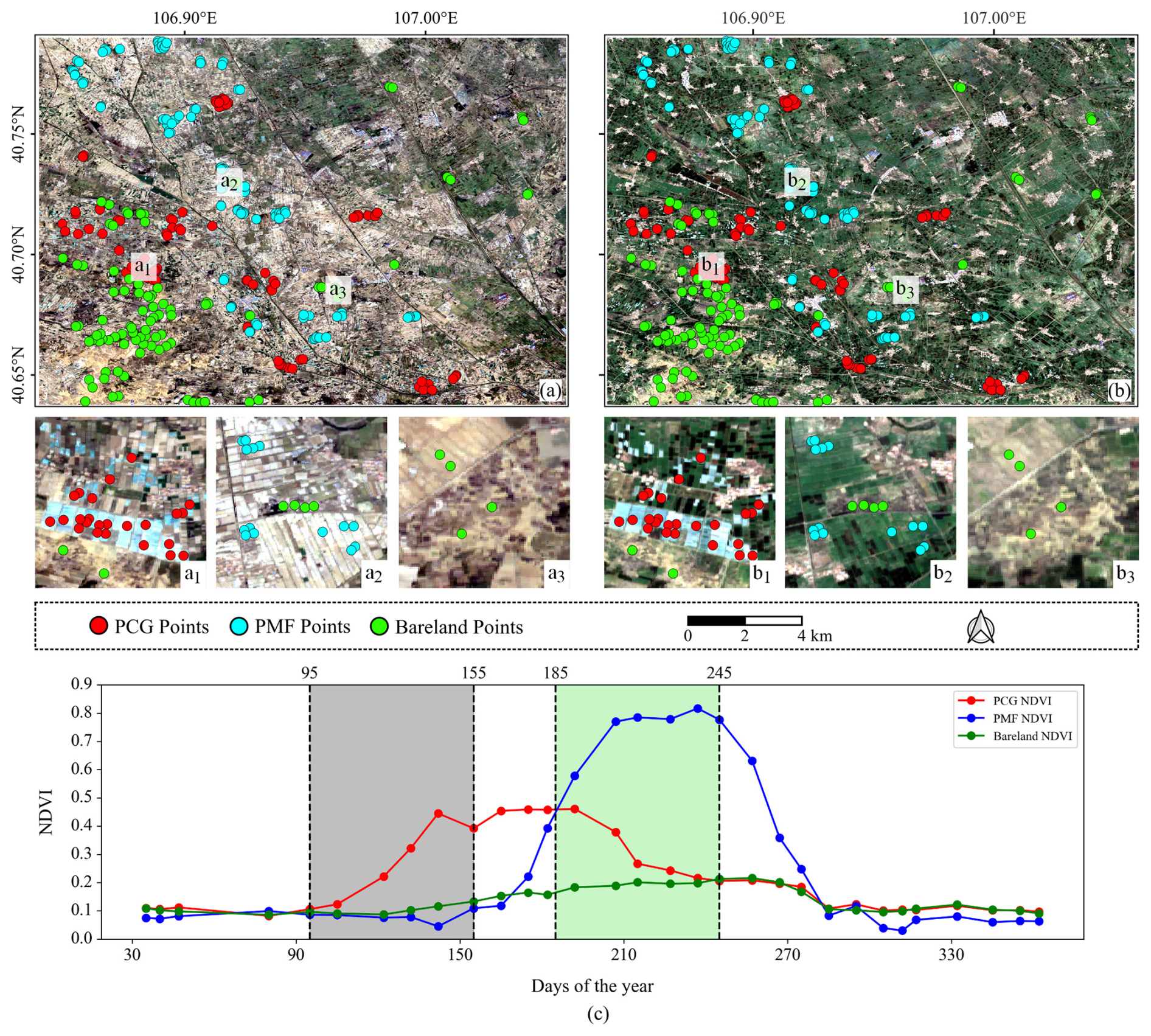
Figure 4 Multi-temporal NDVI profile of bareland, PCGs and PMFs in a representative sub-region of Gansu Province, China. (a) Sentinel-2's spring true color image. (b) Sentinel-2's summer true color image. (c) Time-series NDVI value trend of bareland, PCGs and PMFs.

Based on our previous research (Feng et al., 2022a), using Sentinel-2 satellite data for PCG extraction often encounters confusion with PMFs and bareland. This is mainly due to the spectral similarities among PCGs, PMFs and bareland. To address this issue, we introduced multi-temporal observations to enhance inter-class separability. Here, as an example, we selected 100 sample points for PCGs, PMFs and bareland in part of Gansu province, Northwest China (Fig. 4), which belongs to the single-cropping region. From the NDVI time-series spectral curves in 2020 (Fig. 4c), it is observed that both spring (highlighted in grey) and summer (highlighted in green) witness the differences between PCGs, PMFs and bareland. As a result, we selected multi-spectral Sentinel-2 images in spring (April–June) and summer (July–September) periods as input data in this study area. By incorporating multi-temporal data, we can mitigate the effect of feature confusion in single time-phase images, and get more precise PCG classification results. Meanwhile, Ou et al. (2021) adopted a similar approach by utilizing phenological characteristics to extract PCGs in double-cropping regions.

3.1.2 Feature extraction

The role of feature extraction is to transform remote sensing data from the original pixel space to the feature space, in which the difference and separability of PCG and non-PCG would be further enlarged. Specifically, a multi-dimensional and robust feature space is constructed considering the integration of spectral features and texture features.

1. Spectral features: according to our previous study (Feng et al., 2022a) and other relevant researches (Ou et al., 2021; Zhang et al., 2022a), we mainly consider the following spectral indices, including Normalized Difference Vegetation Index (NDVI) (Huang et al., 2021), Soil Adjusted Vegetation Index (SAVI) (Huete, 1988), Normalized Difference Built-up Index (NDBI) (Zha et al., 2003) and Modified Normalized Difference Water Index (MNDWI) (Xu, 2006). Moreover, several recently published PCG indexes are also included, consisting of PMLI (Lu et al., 2014), APGI (Zhang et al., 2022a), PGHI (Ji et al., 2020), PGI (Yang et al., 2017), and RPGI (Yang et al., 2017).

2. Textual features: it should be noted that PCGs have very distinct geometrical and textual characteristics, manifesting a rather regular rectangular appearance. Therefore, the inclusion of textual features could assist in the separation of PCG from non-PCG. Specifically, we consider the six widely used textural features that derived from grey-level co-occurrence matrix (GLCM), including mean (MEA), standard deviation (STD), homogeneity (HOM), dissimilarity (DIS), entropy (ENT) and angular second moment (ASM).

3.1.3 Random Forest

Random Forest (RF) is utilized as the PCG classification model to generate the initial samples. RF belongs to an ensemble learning method while the base classifier is decision tree. The final output of RF is determined by the majority vote from all the decision trees involved. RF modeling involves two random selection steps. Firstly, the training samples of each base decision tree is randomly selected through bootstrapping. Secondly, the features used to split each node of the decision tree is also randomly selected. These two random processes effectively increase the robustness of RF on multi-dimensional data, and enable RF to cope with collinearity where the latter is an unavoidable issue in remote sensing data. Due to its simplicity and robustness, RF has been widely adopted in remote sensing applications such as urban vegetation mapping, water extraction, crop classification and achieves promising performance (Mei et al., 2024; Sui et al., 2022; Zhang et al., 2024a). In this study, the RF classifier was configured using the ee.Classifier.smileRandomForest( ) function in GEE, the parameters set as follows: numberOfTrees was set to 150, and variablesPerSplit was set to 4.

3.2 Stage-2: coarse-to-fine PCG classification via deep learning

3.2.1 APC-Net model

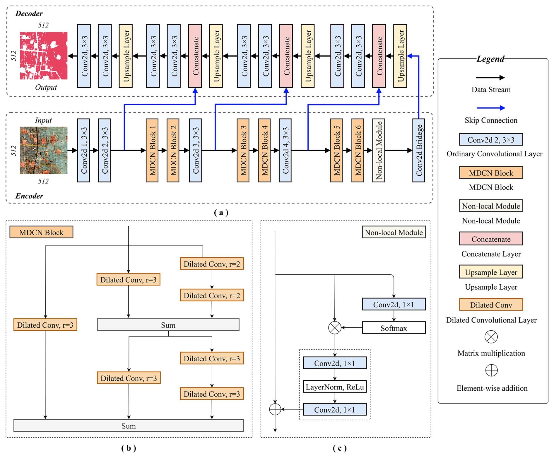
This study utilized our previously proposed deep semantic segmentation model, APC-Net (Niu et al., 2023a), as the core model to generate the final PCG classification map in a coarse-to-fine manner. APC-Net effectively integrates local and global features through multi-scale feature learning, thereby enhancing its classification capability under complex global terrain conditions.

Specifically, APC-Net consists of two main components, an encoder and a decoder (see Fig. 5a). The encoder, which is the core of the network, takes a 512×512 pixels remote sensing image patch as input and extracts highly representative features through a multi-layer structure. This not only enhances intra-class consistency but also improves inter-class separability. The encoder includes convolutional layers, an MDCN (Multi-scale Dilated Convolutional Network) module and a non-local module. The MDCN module (Fig. 5b) integrates multi-scale dilated convolutions to effectively capture multi-scale local features, addressing scale variation issues that are common in PCG classification. The non-local module (Fig. 5c) focuses on capturing global contextual information, thereby improving the model's capability for overall scene understanding. The decoder is responsible for restoring spatial information from the downsampled feature maps generated by the encoder and producing the final segmentation map. It employs bilinear interpolation for upsampling and skip connections to fuse encoder features, further refining the representation. The final PCG classification output maintains the same spatial resolution (512×512 pixels) as the input image.

Figure 5 Overview of proposed APC-Net model.

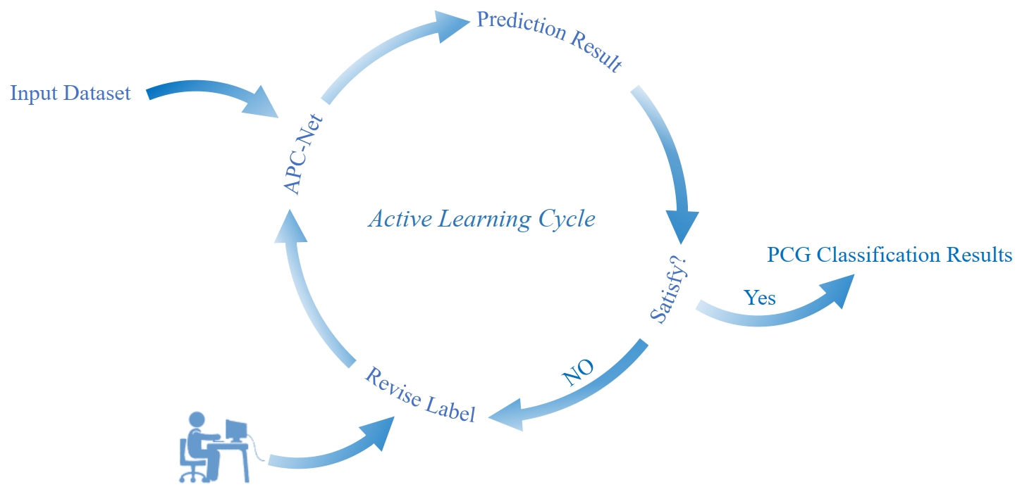
3.2.2 Active learning strategy

In this study, the active learning strategy is employed to optimize initial labels by refining and reorganizing via human intervention. It aims to reduce the false-positive rate hence to improve the classification accuracy. It works as follows. First, the APC-Net model is trained on the initial weak labels (Input Dataset in Fig. 6), which are generated from the RF classifier, and saving the best model weights. Then, these weights are applied to predict the results of the input dataset, producing a set of updated labels. Subsequently, the classification performance is evaluated according to both accuracy evaluation and visual inspection. If the results do not meet the expected standard, initial labels with significant updates are selected to form a new input training dataset. The process is repeated until satisfactory results are achieved, or until performance stabilizes with no further improvements.

Figure 6 Active learning strategy utilized.

The active learning process was conducted for up to five iterations. Each iteration involved complete model training and evaluation using a validation set, with a focus on Overall Accuracy (OA) and mean Intersection over Union (mIoU). To determine whether to proceed with further iterations, we applied a quantitative stopping criterion: if the improvements in both OA or mIoU between two consecutive iterations were less than 1 %, the process was considered to have reached stability and was terminated. For each iteration, candidate samples requiring human intervention were selected based on patch-level disagreement between the model predictions and the initial weak labels. Specifically, a 512×512 pixels image patch was flagged for review if the Patch-level IoU between the predicted label and the initial label was below 0.6. This threshold was determined empirically and reflects a significant discrepancy between model and label, potentially indicating labeling errors or ambiguous regions. Human annotators then manually reviewed these flagged patches. If inconsistencies were confirmed, the incorrect labels were corrected and incorporated into the next round of training. This iterative optimization enabled the model to learn from the most informative and problematic samples, effectively improving both label quality and model performance. When the model achieves an Overall Accuracy (OA) above 90 % and a mean Intersection over Union (mIoU) above 0.6 on the validation set, we consider it to have met the expected classification standard. However, these metrics are only used as reference thresholds for acceptable performance; the final quality of the classification results still requires further evaluation through visual interpretation.

In summary, this Patch-level, IoU-based sample selection and iterative human–machine collaboration ensured that only the most reliable and meaningful corrections were introduced into the training dataset, thereby refining the PCG classification results and reducing the noise introduced by the initial weak labels.

3.2.3 Training details

In this section, we provide a detailed description of the model training process, including the design of the hybrid loss function, the choice of optimizer and the configuration of model hyperparameters. Specifically, this study combines Cross Entropy Loss (CE Loss) and Dice Loss to create a hybrid loss function for the PCG semantic segmentation task. In this hybrid loss function, CE loss primarily measures the discrepancy between labels and model predictions, while Dice loss mitigate the issue of class imbalance, ensuring robust model performance even dealing with underrepresented categories.

$$\begin{array}{}\text{(1)}& {\displaystyle }& {\displaystyle }\mathrm{CE}\mathrm{Loss}=-{\displaystyle \frac{\mathrm{1}}{N}}\sum _{i=\mathrm{1}}^{N}y,\log \left(p_i\right)+\left(\mathrm{1}-y_i\right)\log \left(\mathrm{1}-p_i\right)\text{(2)}& {\displaystyle }& {\displaystyle }\mathrm{Dice}\mathrm{loss}=\mathrm{1}-{\displaystyle \frac{\mathrm{2}\sum _{i=\mathrm{1}}^N{y}_i{p}_i+\mathit{\epsilon }}{\sum _{i=\mathrm{1}}^N{y}_i^{\mathrm{2}}+\sum _{i=\mathrm{1}}^N{P}_i^{\mathrm{2}}+\mathit{\epsilon }}}\end{array}$$

where N denotes the number of samples, y_i is the true label of the ith sample, p_i is the corresponding predicted probability, and ε is a very small constant in case of a division by zero error.

A hybrid loss function is designed by combining the merits of CE loss and Dice loss for semantic segmentation. The formula as follows, where α represents the weight ratio between the two loss terms, equals to 0.2.

$$\begin{array}{}\text{(3)}& \mathrm{Hybrid}\mathrm{Loss}=\mathit{\alpha }\times \mathrm{CE}\mathrm{Loss}+(\mathrm{1}-\mathit{\alpha })\times \mathrm{Dice}\mathrm{Loss}\end{array}$$

The APC-Net model was implemented using the PyTorch 1.12.1 framework and trained on a GPU of NVIDIA GeForce RTX 3090 (24 GB), with an Intel Core i7-12700KF CPU@5.00 GHz and Ubuntu 20.04 operating system. The widely used Adam optimizer was applied with an initial learning rate of $\mathrm{1}\times {\mathrm{10}}^{-\mathrm{4}}$, followed by a step decay schedule. The model was trained for 200 epochs with a batch size of 8, and early stopping was applied with a patience of 10 epochs based on validation loss to prevent overfitting.

To construct the training and validation datasets, we collected a total of 18 532 samples, each with a resolution of 512×512 pixels. Specifically, 10 230 samples were collected from China, and 8302 from other regions. Given that PCG areas in China account for more than two-thirds of the global total, we divided the dataset into two geographic subsets (China and non-China) to mitigate overfitting and allow the model to learn region-specific features. Each subset was randomly split into training and validation sets using an 8:2 ratio, resulting in 14 825 training samples and 3707 validation samples in total.

To enhance the global representativeness of the model, PCG sample collection covered major agricultural regions across six continents, including Asia, Europe, North America, South America, Africa, and Oceania. Two separate regional models were trained using the respective subsets, and their predictions were finally combined to produce the Global-PCG-10 dataset, a global 10 m resolution PCG classification product.

3.3 Accuracy assessment

We adopt both qualitative and quantitative accuracy assessment to justify the classification performance of Global-PCG-10. The former is to compare Global-PCG-10 with remote sensing images to check the obvious classification errors, while the latter is to calculate a series of accuracy metrics including overall accuracy (OA), recall, precision, F₁-score, etc. Actually, OA is derived from the confusion matrix that are calculated in the test dataset, whose formulas are as follows.

$$\begin{array}{}\text{(4)}& \mathrm{OA}={\displaystyle \frac{\mathrm{1}}{N}}\sum _{i=\mathrm{1}}^r{x}_{ii}\end{array}$$

where N denotes the total number of samples, r represents the number of classes, and x_ii refers to the diagonal elements of the confusion matrix.

Considering that PCG mapping belongs to a binary classification problem, therefore, the widely used metrics in binary classification such a recall, precision and F₁-score would also be a good choice to justify the performance of Global-PCG-10. These metrics have also been used by Fu et al. (2021), where the three metrics are used for the accuracy evaluation of China's marine aquaculture mapping results.

$$\begin{array}{}\text{(5)}& {\displaystyle }& {\displaystyle }\mathrm{precision}={\displaystyle \frac{\mathrm{TP}}{\mathrm{TP}+\mathrm{FP}}}\text{(6)}& {\displaystyle }& {\displaystyle }\mathrm{recall}={\displaystyle \frac{\mathrm{TP}}{\mathrm{TP}+\mathrm{FN}}}\text{(7)}& {\displaystyle }& {\displaystyle }{F}_{\mathrm{1}}={\displaystyle \frac{\mathrm{2}\times \mathrm{precision}\times \mathrm{recall}}{\mathrm{precision}+\mathrm{recall}}}\end{array}$$

where TP represents true positives, i.e., the number of correctly classified PCG pixels, FN denotes false negatives, i.e., the number of PCG pixels misclassified into non-PCG, while FP stands for false positives, i.e., the number of non-PCG pixels misclassified into PCG. In general, recall and precision are contradictory to each other. A high recall also brings in a high FP, which would lead to low prevision. On the other hand, F₁-score is an integrated index that takes into consideration of both recall and precision. F₁-score has a value between 0 and 1, where a higher F₁-score means a better classification performance.

4 Results and discussion

4.1 Spatial pattern of Global-PCG-10

Figure 7 illustrates the global distribution of PCGs in the mapping unit of 0.1° grid instead of using per-pixel PCG classification results. This is because the predicted PCGs cover only a small fraction of the entire globe. If we put the per-pixel results on map, PCGs would be overwhelmed by background regions. To tackle this issue, we change the mapping unit from per-pixel (i.e., 10 m) to 0.1° grid through zonal analysis, which could enhance the visual effect of PCGs spatial distribution globally.

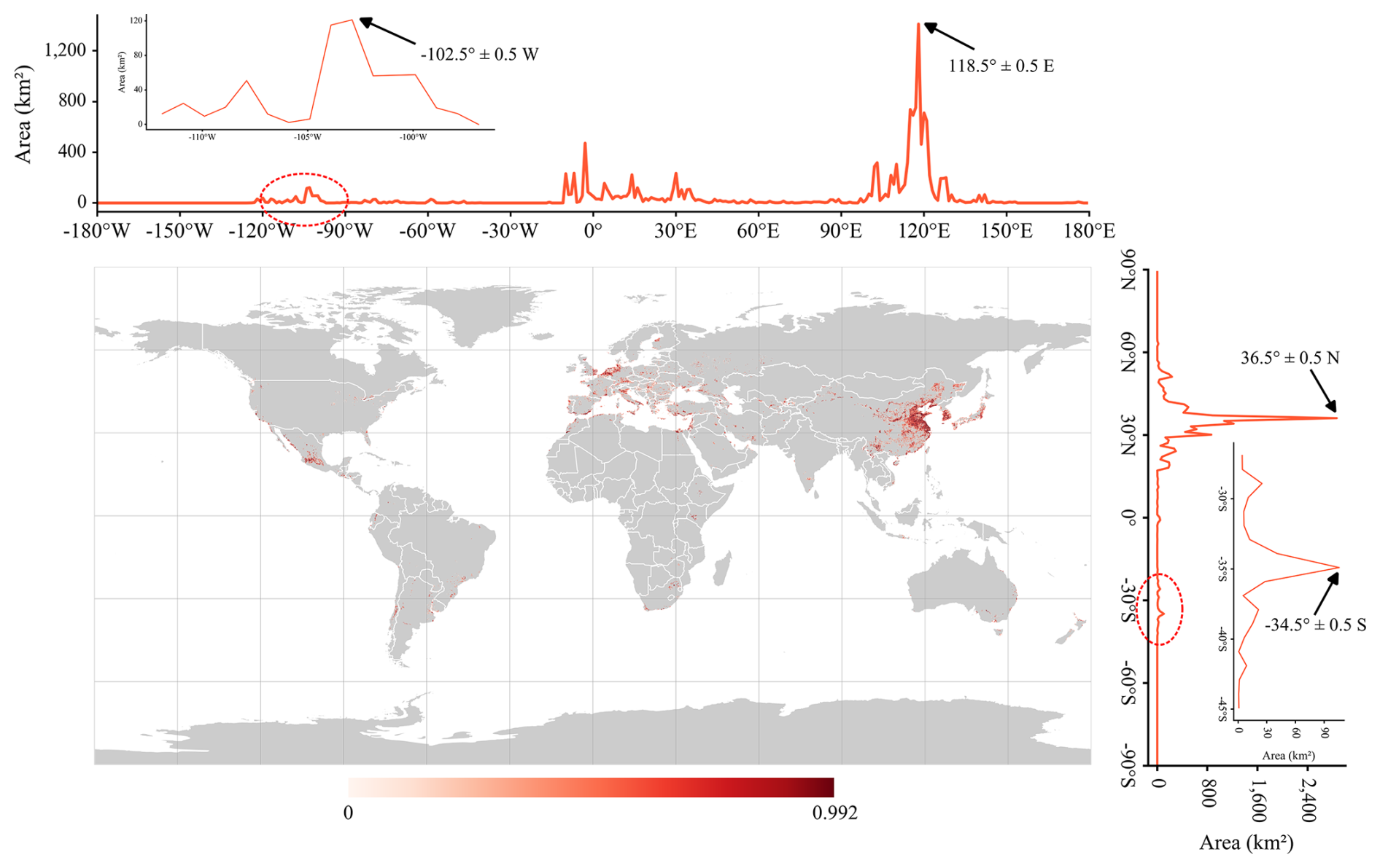
Figure 7 Global PCG spatial distribution in 2020. The spatial resolution of the map is 0.1°.

As depicted in Fig. 7, the global PCGs mainly locate in East Asia and Mediterranean regions. Specifically, in East Asia, China has the largest area of PCGs, where most PCGs are clustered in North China Plain (Eastern China), Liaohe Plain (Northeastern China), Sichuan Basin and intermountain basin of Yunnan Province (Southwestern China). In Mediterranean region, PCGs are mainly distributed along the coasts in Iberian Peninsula, Apennine Peninsula, Balkan Peninsula and Nile Delta. The widespread presence of PCGs in these regions, where are characterized by both a well-developed and a long history of farming, can be attributed to two key factors. First, the use of PCGs allows for the expansion of both acreage and production of high-quality vegetables, fruits, flowers, and other cash crops. This is particularly beneficial in China, where it could effectively increase income of local farmers. Second, most of these PCGs are located in plains or basins, close to urban areas, and have relatively abundant water resources. These geographic advantages provide favorable conditions for irrigation and product marketing, which could help to ensure the efficiency and output of facility-based agriculture.

Meanwhile, Fig. 7 also witnesses several regions with nearly no PCGs, including North America, Northern Eurasia, Sub-Saharan Africa and Oceania. Two reasons may account for this. On one hand, in North America, the agricultural mode is large farms facilitated with advanced agricultural machinery and less workers. Considering that PCGs are rather labor intensive and not easy for machinery to work, therefore, they are not widespread in both United States and Canada. On the other hand, in areas like South America, sub-Saharan Africa, Northern Eurasia and Oceania, the lower level of agricultural development and limited infrastructure hinder the adoption and growth of PCGs. Additionally, in China and along the Mediterranean coast region, profit-driven small holders are the majority. Under this circumstance, together with policy incentive, farmers choose to build PCGs to produce cash crops, leading to the prevalence of PCGs in these regions.

In addition, we calculate the PCG area along both longitude and latitude in an interval of 1° and depict the area histogram in Fig. 7. It indicates that the global PCGs mainly locate in the Northern Hemisphere, especially between 30 and 40° N with a peak at about 36° N, which accounts for 65.84 % of the total PCG area. Meanwhile, these regions just correspond to North China Plain and Mediterranean region. From the perspective of longitude, most PCGs are clustered in the Eastern Hemisphere, while the Western Hemisphere only witnesses a high PCG density on the west side of the Mexican Plateau, the west side of the Chilean Cordillera, and the La Plata Plain (river inlets) of Argentina.

Moreover, we calculate both the total area of PCGs (Fig. 8a) and the ratio of PCG area to cropland area in each country (Fig. 8b). The former reflects the production scale of PCGs while the latter stands for the proportion or importance of PCGs in local agricultural activities. As shown in Fig. 8a, the total area of global PCGs reached to 14 259.85 km² in 2020, while Asia has the largest PCG area of 9874.51 km², accounting for 69.24 % of the total global PCGs. Europe ranks the second with a PCG area of 2530.56 km² and a PCG ratio of 17.75 %. North America, Africa, South America and Oceania witness a decent PCG area of 819.12, 668.82, 213.92 and 152.91 km², respectively. From the perspective of country, China ranks the first with a PCG area of 8224.90 km². Meanwhile, China accounts for 83.29 % of PCGs in Asia and 57.67 % in the globe. Spain ranks the second in the world and the first in Europe with a PCG area of 803.26 km². Other countries with a PCG area over 500 km² include Mexico, Italy and South Korea. On the contrary, countries in Sub-Saharan Africa, Central Asia and other countries like Mongolia, Russia, United States and Canada, have very few PCGs.

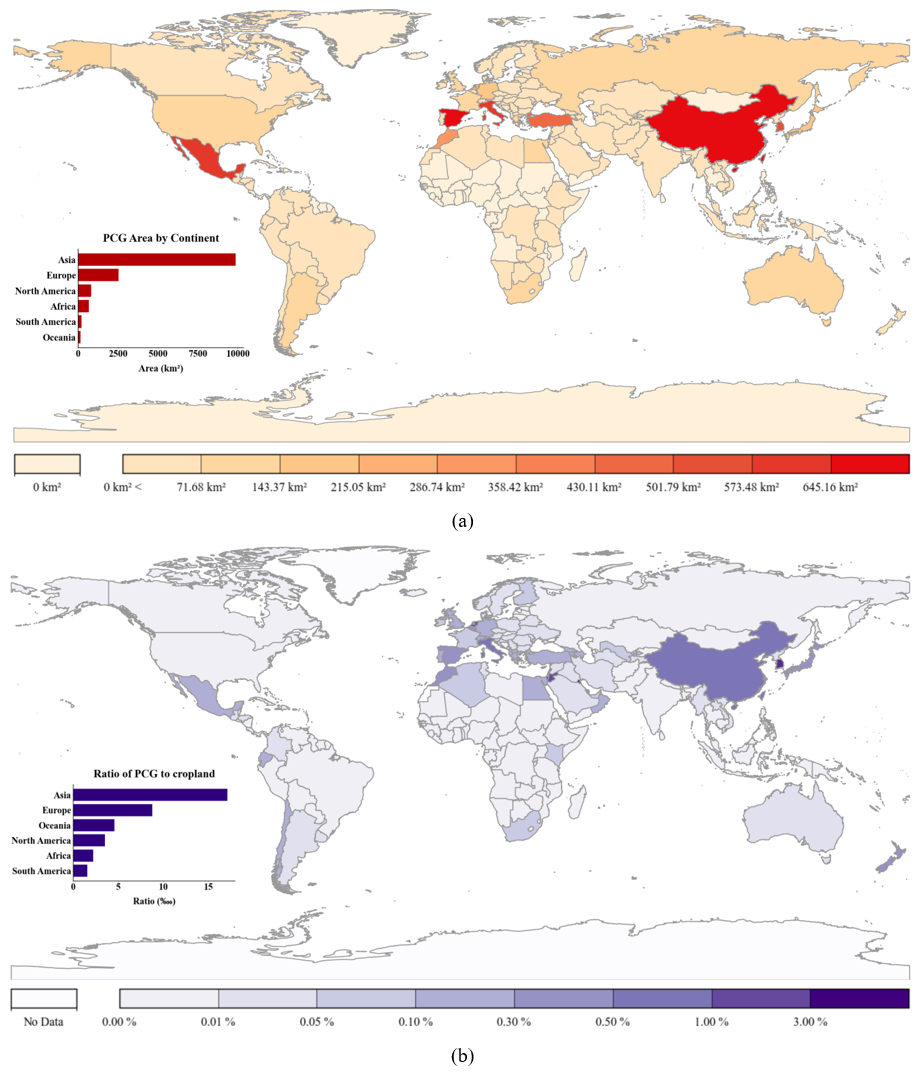
Figure 8 PCG area statistic mapping in 2020. (a) Area of PCGs. (b) Ratio of PCGs to cropland.

Figure 8b illustrates the ratio of PCG area to cropland. It indicates that although China has the largest PCG region, its PCG ratio (0.64 %) is relatively lower. The country with the highest PCG ratio is Kuwait (5.23 %). Other Mediterranean countries such as Italy and Turkey also have a relatively higher PCG ratio. In Eastern Asia, South Korea has a high PCG ratio although they have small PCG regions, which manifests the important role of PCGs in these countries. The main reason is that these countries are mostly situated in mountainous, hilly or Gobi terrain conditions, leading to a limited amount of usable cropland. In such conditions, PCGs, as a form of intensive facility-based agriculture, can overcome the limitations of the local natural climate. It also effectively optimizes the structure of the local agriculture industry, increases the diversity of agricultural products, and reduces reliance on imported fruits, vegetables, and other cash crops.

4.2 Reliability of Global-PCG-10

This section would analyze and justify the reliability of Global-PCG-10 from both visual inspection and accuracy assessment results. Here, we present both the remote sensing images and the corresponding Global-PCG-10 maps from several typical regions across the world, including Shouguang of China, Lam Dong of Vietnam in Asia; Almeria of Spain, Ragasu of Italy in Europe; Outlet of Morocco, Damous of Algeria in Africa; Samis of the US, Zapotitan of Mexico in North America; Lisandro of Argentina, Bom Repouso of Brazil in South America; Robinvale of Australia, Manngatepere of New Zealand in Oceania. As shown in Fig. 9, our classification results are excellent in regions with a high density of greenhouses, with virtually no noticeable omission of PCGs. Furthermore, no significant false-positive errors were observed, even in areas with a sparse distribution of PCGs (e.g., the United States, Brazil, etc.). Additionally, Global-PCG-10 demonstrates reliable recognition of PCGs in various global climate zones, including humid climates, Mediterranean climates, and others.

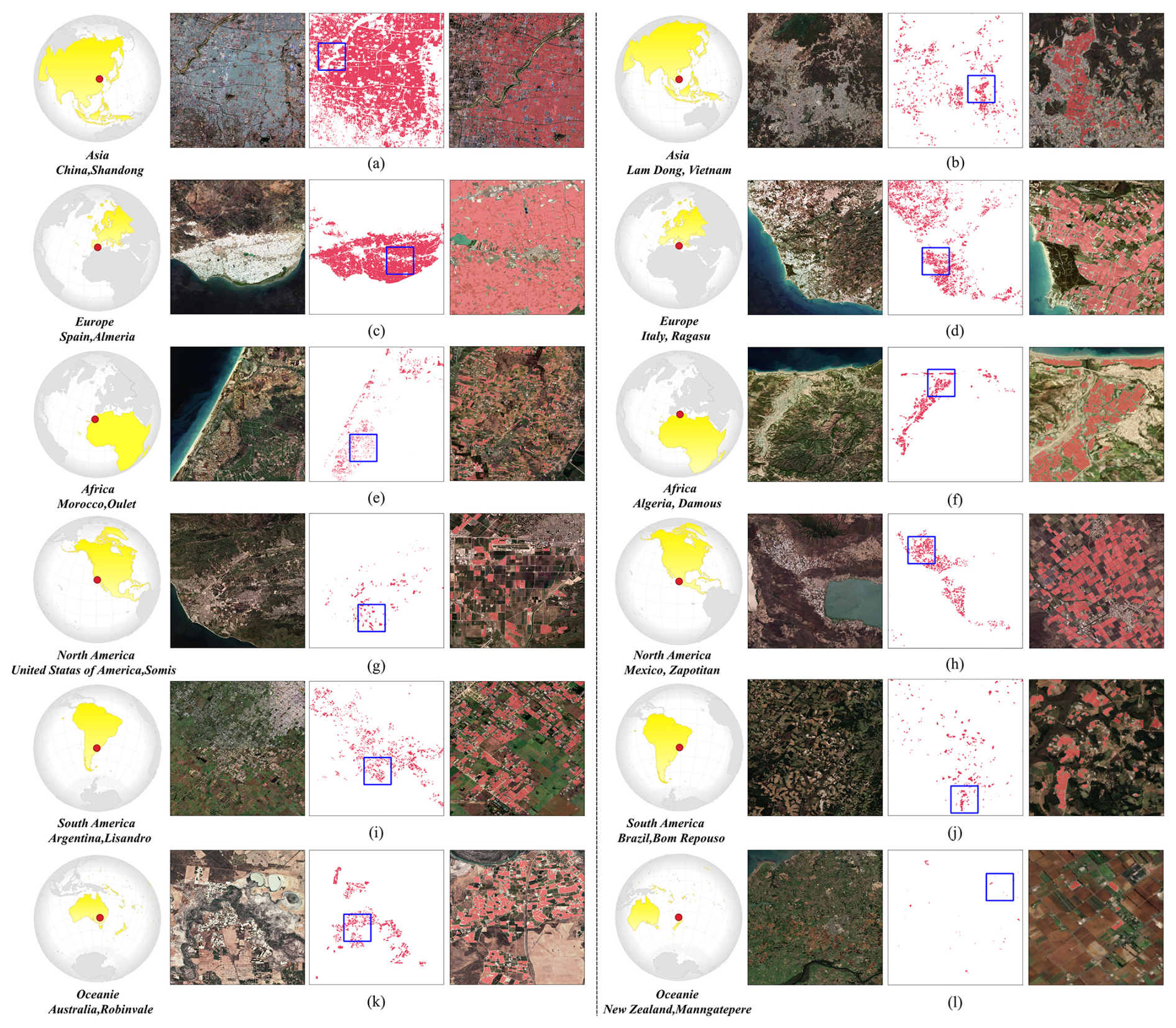
Figure 9 Details of the Global-PCG-10 map. (Note: taking (a) as an example, from left to right is the location in the world, RGB Sentinel-2 image, Global-PCG-10 map and detailed fused mapping result of the blue rectangle region.)

Details of Global-PCG-10 illustrate that we have achieved a very good PCG map with accurate and neat boundaries under the spatial resolution of 10 m. The confusion between PCGs and non-PCGs is not obvious and the speckle noises in the background have been greatly suppressed. Two reasons may account for this. First, the utilization of multi-temporal Sentinel-2 satellite image could reduce the misclassification and “salt and pepper effect” caused by PMFs, bareland, and other land cover classes. Second, the PCG classification framework, which integrates active learning strategy into the deep learning model, enables a coarse-to-fine classification process.

To further quantitatively evaluate the reliability of the Global-PCG-10 dataset, we constructed a dedicated test sample set. The spatial distribution of test samples is shown in Fig. 10.

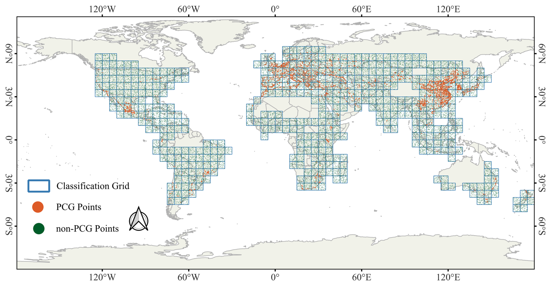
Figure 10 Spatial distribution of global test samples.

The dataset includes two categories, PCG and non-PCG. Based on previous research practices (Olofsson et al., 2013, 2014; Tian et al., 2025; Wang et al., 2023), we followed the stratified random sampling strategy recommended by Olofsson et al. (2014), in which samples were drawn in proportion to the mapped area of each class within the actual mapping region. However, since the global coverage of PCG is less than 1 %, strictly proportional sampling would result in too few PCG samples to support a statistically robust accuracy assessment. To address this issue, and consistent with the approaches adopted in the above studies, we moderately increased the proportion of PCG samples in the test set to approximately 10 %. This adjustment could enhance the evaluation capability for this minority class.

As shown in Table 1, the total number of test samples is 46 000, with 6000 PCG samples and 40 000 non-PCG samples. To ensure the validity, we applied separate sampling strategies for each category. As for PCG, test samples were derived from the global 3 m PCG dataset in 2019 developed by Tong et al. (2024), and manually verified through Google Earth visual interpretation. Since the Global-PCG-10 dataset is for the year 2020, and considering that PCGs typically have long lifespans and stable structures, the 2019 dataset by Tong provides a reliable reference. Additionally, we performed a second round of verification using historical Google Earth imagery in around 2020 to confirm their existence and status, minimizing sampling bias from prior knowledge. And for non-PCG, due to the large quantity required, manual sampling was impractical. We thus randomly sampled non-PCG from the GLC_FCS30D dataset to ensure independence and randomness. All samples were also verified through visual interpretation of historical Google Earth imagery in around 2020 to ensure label correctness.

Table 1 Confusion matrix.

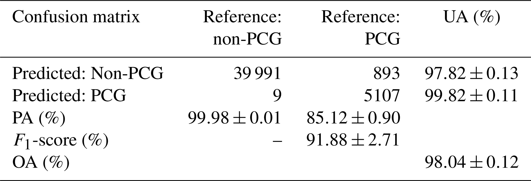
Note: PA, Producer's Accuracy; UA, User's Accuracy; OA, Overall Accuracy.

Based on this test dataset, Global-PCG-10 achieved a PA of 85.12 % ± 0.90 %, a UA of 99.82 % ± 0.11 %, an F₁-score of 91.88 % ± 2.71 % and an overall accuracy of 98.04 % ± 0.12 % (Table 1). In the revised confusion matrix, the bias for non-PCG has been effectively reduced. However, PCG still exhibits a gap between precision and recall, characterized by a high precision but a low recall. This may be caused by missed detections of small PCG patches. Unlike PlanetScope, Sentinel-2 has lower spatial resolution with 10 m, and small PCG often spans only a few mixed pixels, making it difficult to extract meaningful spectral features for accurate PCG classification. The high precision, on the other hand, is likely due to post-processing applied to the initial classification results. Among these steps, the Sieve Filter method played a key role by removing small, erroneous regions through multi-level filtering, thereby improving the quality of PCG predictions and enhancing precision. Specifically, we used the gdal.SieveFilter( ) function from the GDAL library (invoked in the Python environment) to perform the filtering. An 8-connected neighborhood was adopted, and a set of hierarchical thresholds for the minimum number of connected pixels (10/20/50) was applied. This multi-level threshold setting was designed to accommodate variations in noise distribution and mapping requirements across different regions.

In Table 1, the relatively high number of false negatives (FN = 893) can be attributed to the following factors.

1. Omission of small-scale PCG targets. Due to the 10 m spatial resolution of Sentinel-2 imagery, which is significantly lower than that of high-resolution platforms like PlanetScope, small PCG often occupies only a few to a dozen pixels and are easily affected by mixed pixel issues. This makes it difficult for the model to extract reliable spectral features and leads to missed detections.

2. Limitations in spatiotemporal coverage of imagery. The Sentinel-2 data used in this study were organized by 1° grid tiles. Due to cloud contamination and observation scheduling constraints, it is sometimes challenging to obtain cloud-free imagery for both time periods (spring and summer), which reduces the model's ability to detect PCG in certain regions.

3. Post-classification filtering effects. To reduce false positives, we applied a strict post-processing procedure to the initial classification results when generating the Global-PCG-10 dataset. Specifically, a multi-stage Sieve Filter was used to remove small patches and isolated noise, which effectively suppressed misclassifications and significantly improved the precision (UA) for the PCG class.

Additionally, based on the test samples and a systematic comparison with the 3 m resolution PCG data provided by Tong et al. (2024), we identified two main types of omission errors in the current Global-PCG-10 dataset during the PCG extraction process, as detailed below.

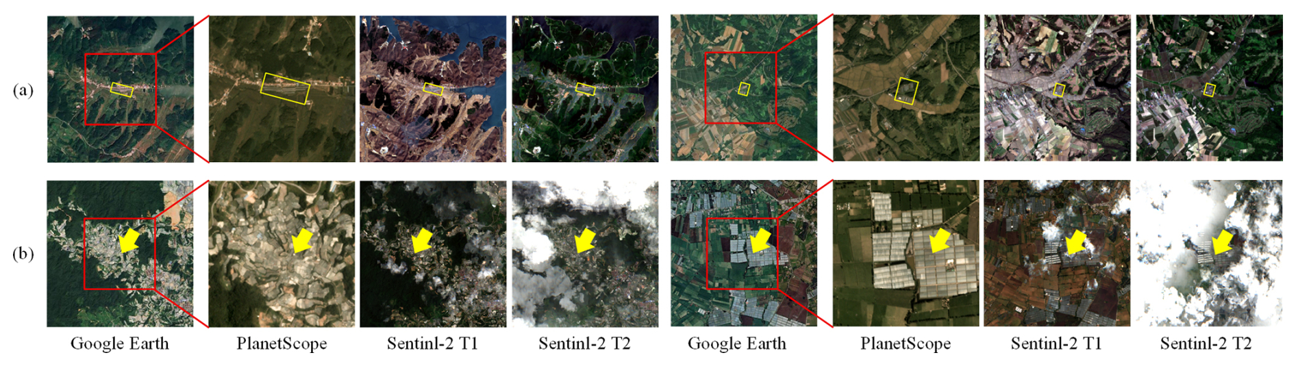
Figure 11 Bad case analysis. (Note: from left to right, the image shows the © Google Earth imagery from 2020, 3 m spatial resolution PlanetScope imagery from 2019 and Sentinel-2 imagery from spring and summer, respectively.)

As shown in Fig. 11a, due to the relatively coarse spatial resolution (10 m) of Sentinel-2 imagery compared to higher resolution sources such as PlanetScope or Google Earth (3 m or finer), small-scale PCG targets often occupy only a few to a dozen pixels. These pixels are usually mixed pixels that contain spectral information from multiple surrounding land cover types. As a result, the model finds it difficult to extract PCG's distinct spectral and texture features, which impairs its ability to accurately detect small and visually inconspicuous PCG. For instance, in the area shown in Fig. 11a, the PCG can be roughly identified in the high-resolution image, with some observable texture patterns. However, in the corresponding Sentinel-2 image at 10 m resolution, the PCG contours are blurred and lack clear geometric and textural features, leading to missed detections.

Meanwhile, the Global-PCG-10 dataset is derived using multi-temporal Sentinel-2 imagery from spring and summer, organized by 1° grid tiles. However, due to cloud contamination and limited observation opportunities, it is challenging to obtain cloud-free images for both seasons in some regions (Fig. 11b). This could limit the model's ability to extract consistent temporal features, thereby increasing the likelihood of omission errors. Figure 11b presents a typical case, although the overall cloud coverage is relatively low, even thin clouds can affect surface reflectance values and interfere with the model's classification performance.

In summary, misclassification errors in PCG classification primarily arise from two aspects: (1) the presence of mixed pixels in medium-resolution imagery when detecting small-scale PCG, which weakens the model's ability to learn effective spectral and textural representations; and (2) limitations in the spatial and temporal availability of remote sensing data, particularly due to cloud cover and long revisit intervals, which may result in missing key seasonal observations and reduce classification accuracy.

4.3 Comparison with other studies

4.3.1 Comparison with global LULC dataset

As a distinct land cover category, PCGs should belong to cropland. However, to the best of our knowledge, PCG has not been fully considered in previously released global LULC datasets. Therefore, in this section, we compare our Global-PCG-10 with other released global LULC datasets. To ensure temporal consistency, we only selected LULC datasets containing 2020 data products comparison, including Dynamic World (Brown et al., 2022), ESA World Cover (Zanaga et al., 2021), ESRI Land Cover (Karra et al., 2021), FROM-GLC30 (Yu et al., 2022), and GLC_FCS30D (Zhang et al., 2024c). Among these, Dynamic World, ESA World Cover, and ESRI Land Cover have a spatial resolution of 10 m, while FROM-GLC30 and GLC_FCS30D have a spatial resolution of 30 m. Since the classification system of each dataset is different, this study is based on the land cover types of the selected typical regions and uses GLC_FCS30 as a reference. And the land cover types are unified into the following nine categories: Cropland, Shrubland, Grassland, Bareland, Wetland, Impervious surface, Forest, Water Body and Ice/snow.

As shown in Fig. 12, the left part presents the Sentinel-2 true color images of typical regions along with their corresponding Global-PCG-10 maps, while the right part displays the mapping results from various LULC datasets. It is quite clear that these LULC datasets have low classification performance in PCG regions. Specifically, Dynamic World erroneously classifies PCGs as impervious surfaces (Fig. 12a, b, f and g), Ice/snow (Fig. 12c, d, f and h), and bareland (Fig. 12i). ESA World Cover misclassifies PCGs as impervious surfaces (Fig. 12d and h) and bareland (Fig. 12a, e and i). ESRI Land Cover misclassifies PCGs as impervious surfaces (Fig. 12b, f and i), bareland (Fig. 12d), and grassland (Fig. 12h). FROM-GLC30 misclassifies them as impervious surfaces (Fig. 12a, f, i and j) and grassland (Fig. 12a, b, i and j). GLC_FCS30D similarly misclassifies PCGs as impervious surfaces (Fig. 12d, f and h).

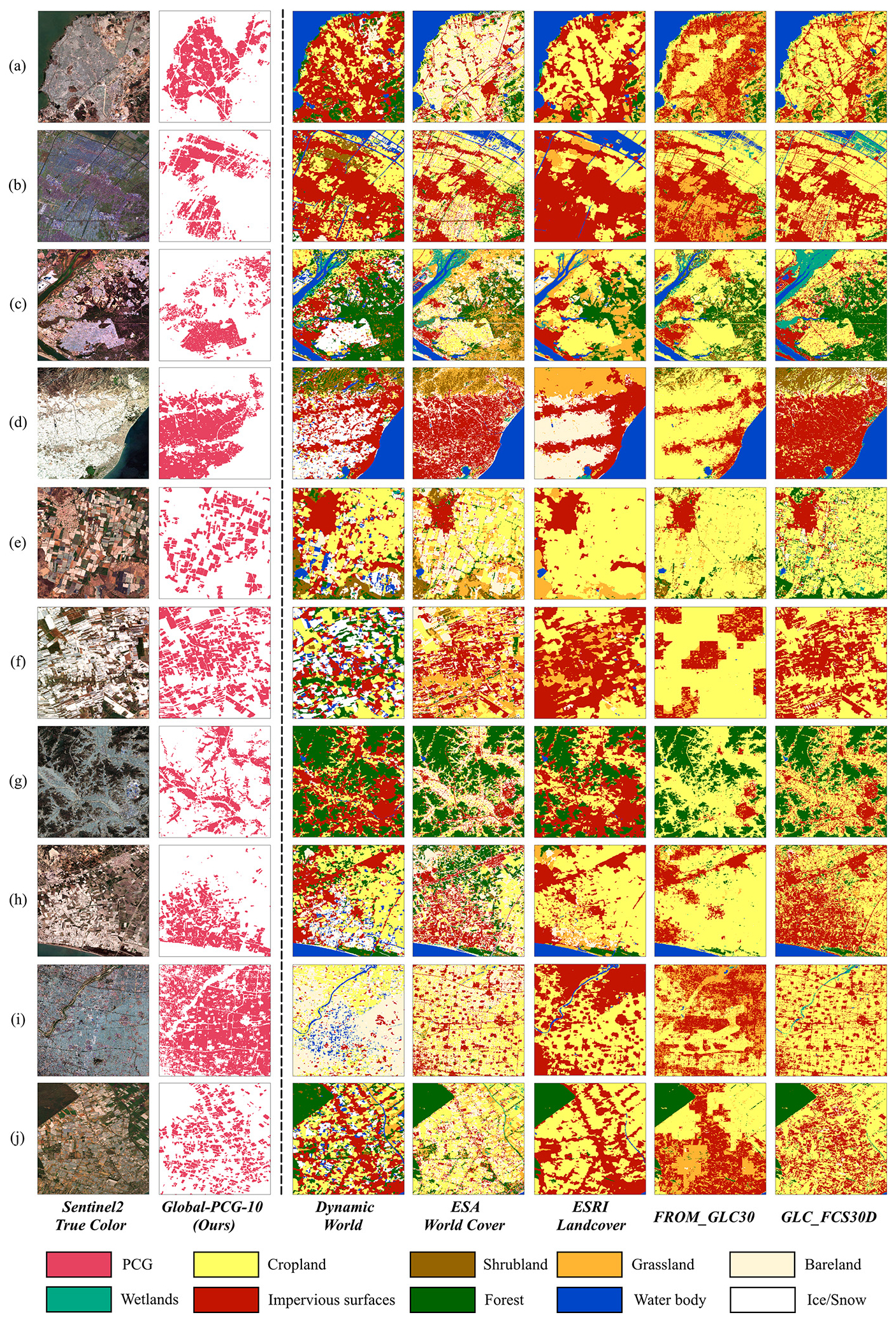
Figure 12 Comparison of Global-PCG-10 with other global LULC products.

Above all, PCGs are commonly misclassified into four categories: impervious surfaces, bareland, grassland, and Ice/snow. Specifically, impervious surfaces and bareland, such as white-roofed factories, villages, and photovoltaic panels, may share similar spectral or texture features with PCGs, leading to obvious misclassification. Additionally, the phenology of crops grown within greenhouses can also affect the spectral features of PCGs, making them resemble grassland at certain times and leading to misclassification. Besides, the reflectance of PCGs in some regions is similar to that of clouds and snow, which might explain why PCGs are sometimes misclassified into these categories.

Meanwhile, Fig. 12 also indicates some LULC datasets exhibit good performance in classifying PCGs into cropland. For instance, Fig. 12b and c of ESA World Cover, Fig. 12a, c and e of ESRI Land Cover, Fig. 12d, e and h of FROM-GLC30, and Fig. 12a–c, e, g and i of GLC_FCS30D. The classification results successfully identify PCGs as cropland with greater precision in these cases.

4.3.2 Comparison with other PCG dataset

Research on large-scale extraction of PCGs includes several excellent efforts. Our previous study released the first 30 m national-scale PCG dataset of China in 2019 (Feng et al., 2022a), and in May 2024, the University of Copenhagen published a global 3 m PCG dataset also in 2019, both of which are open access. Additionally, Wuhan University conducted PCG mapping in 2016 using high-resolution satellite data and deep learning techniques (Chen et al., 2023; Ma et al., 2021), and the Chinese Academy of Sciences conducted a nearly 20-year extraction and spatial analysis of PCGs in China using Landsat 5/8 data on GEE cloud platform (Liu and Xin, 2023; Ou et al., 2019). However, these two studies' datasets have not been publicly released. Therefore, this study conducts a comparison with the 3 m PCG dataset from the University of Copenhagen from both qualitative and quantitative perspectives.

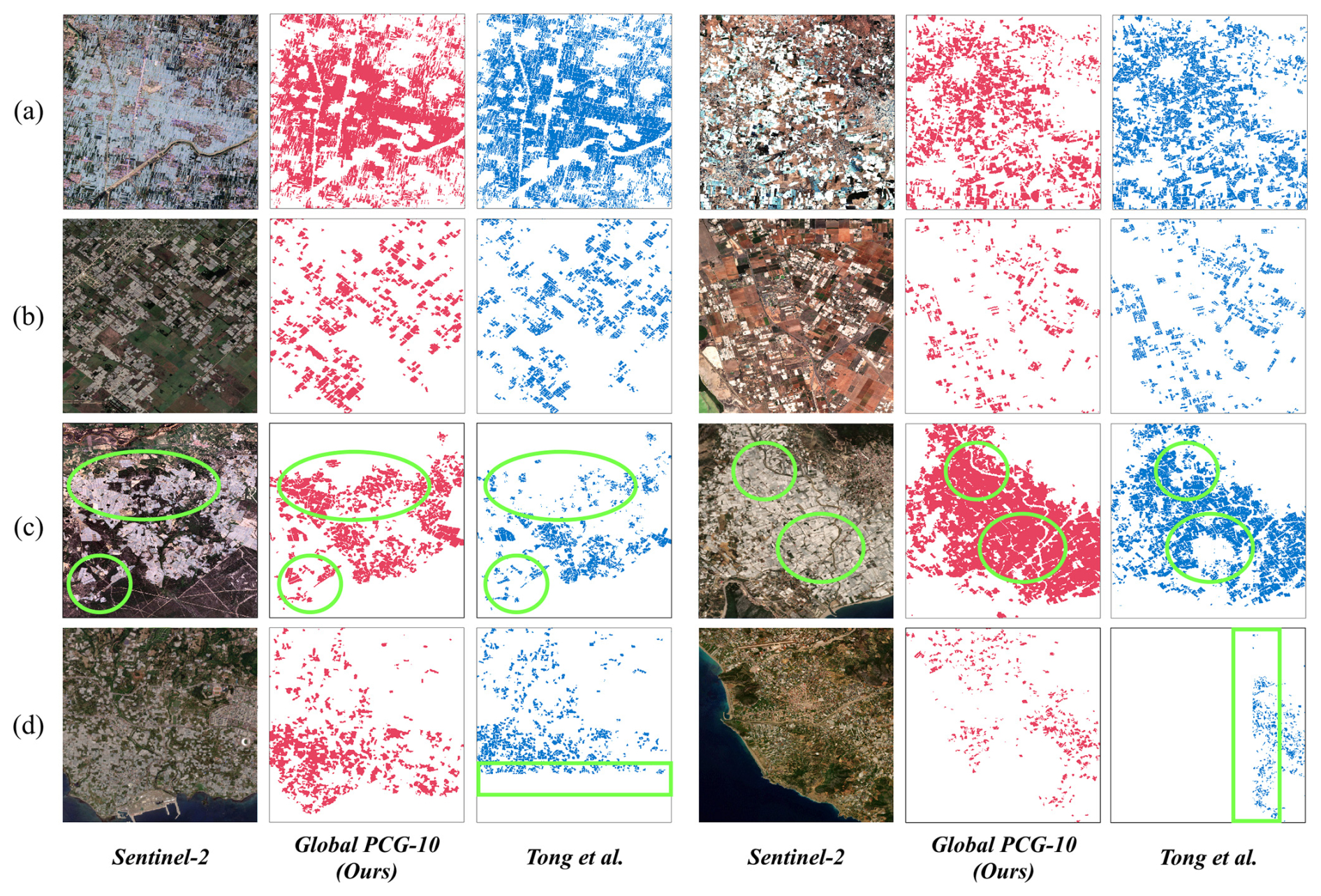
Figure 13 Comparison with other PCG dataset. (Note: light red depicts our Global PCG-10, light blue represents Tong et al. (2024) and green circles/rectangles mark the differences.)

Figure 13a and b illustrates the mapping results in regions with different PCG densities. In Fig. 13a, it shows both datasets exhibit very similar spatial patterns in densely distributed PCG regions. Figure 13b demonstrates that Global-PCG-10 can still accurately capture the greenhouse layout even in areas with sparse PCG distribution, performing on par with Tong et al. (2024) acquired from 3 m commercial satellites. Figure 13c highlights the case where Global-PCG-10 accurately detected greenhouses while Tong et al. (2024) missed. Figure 13d also shows a case of missed detection by Tong's dataset, but unlike Fig. 13c, the missed detection in Fig. 13d is more likely due to missing of satellite image. The rectangle indicates that the data is split into two parts by an “invisible” line. Such situation is commonly caused by improper data organization or gaps of source satellite data. On the contrary, we used Sentinel-2 satellite data, with its dual constellation providing a 5 d revisit cycle, which ensures minimal gaps in remote sensing imagery, thereby delivering high-quality data support for PCG mapping globally.

To provide a more objective and fair comparison, we followed the methodology proposed by Huang et al. (2022) and conducted a quantitative consistency analysis between the two datasets in terms of global PCG spatial distribution. Specifically, we selected four representative 1°×1° grid regions with varying PCG densities. Each of these grids was further subdivided into multiple 0.01°×0.01° sub-grid units. Within each sub-grid, we calculated the proportion of PCG pixels relative to the total number of pixels for both datasets (i.e., PCG area ratio, ranging from 0 to 1). Using these continuous ratio-based data, we applied linear regression analysis to calculate the coefficient of determination (R²), thereby quantifying the spatial distribution consistency between the two datasets across different regions. Unlike methods that rely on discrete classification labels, this approach leverages continuous area proportions, making it more suitable for evaluating agreement between remote sensing datasets with differing spatial resolutions. As shown in Fig. 14a–d, the experimental results indicate that, in high-density PCG regions, our 10 m resolution PCG dataset demonstrates a high degree of spatial consistency with the 3 m reference dataset.

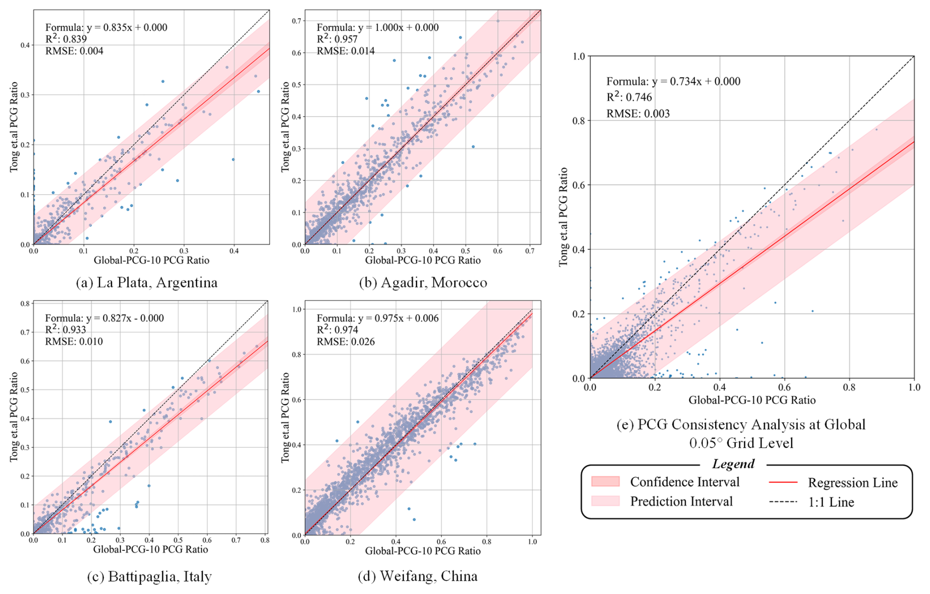
Figure 14 The consistency performance across the four representative regions and between the dataset by Tong et al. (2024) and Global-PCG-10 in representative regions.

To further evaluate spatial consistency at the global scale, we applied a standard regression-based consistency analysis across the entire globe, with reference to the analytical approach and spatial resolution (i.e., 0.05° grid) used by Huang et al. (2022). The coefficient of determination (R²) was again employed as the primary evaluation metric. As shown in Fig. 14e, the comparison based on a 0.05° grid reveals strong agreement in the global spatial distribution of PCG between the dataset published by Tong et al. (2024) and the Global-PCG-10 dataset. The regression analysis yields an R² of 0.746, a root mean square error (RMSE) of 0.003, and a regression equation of $y=\mathrm{0.734}x+\mathrm{0.000}$. These results indicate a moderate to strong spatial correlation between the two datasets, further validating the effectiveness of the Global-PCG-10 dataset in capturing the global distribution pattern of PCG.

As illustrated in Fig. 14, the Global-PCG-10 dataset exhibits strong agreement with the reference data in typical regions (Fig. 14a–d), whereas a moderate overestimation trend is observed at the global scale. This discrepancy may be attributed to the spatial resolution limitations of Sentinel-2 imagery. As a medium-resolution satellite (10 m), Sentinel-2 is more susceptible to intra-class spectral variability and inter-class spectral confusion. In sparely distributed greenhouse areas, non-PCG features such as bare soil, inter-greenhouse roads, or adjacent agricultural structures may exhibit spectral signatures similar to plastic-covered greenhouses, leading to misclassification and systematic overestimation of PCG coverage. Moreover, within the same spatial aggregation unit (e.g., a 0.05° grid cell), Sentinel-2 offers fewer pixels compared to PlanetScope (3 m), making PCG area statistics more sensitive to per-pixel classification errors. Consequently, in typical regions with more homogeneous greenhouse patterns, clearer boundaries, the classification results are more stable and consistent. In contrast, at the global scale, the combined effects of landscape heterogeneity and resolution-induced error propagation contribute to reduced agreement.

4.4 Application potential and limitations of the dataset

As described above, Global-PCG-10 is a global-scale dataset of PCG derived from open-access Sentinel-2 imagery. By leveraging freely available satellite data, the dataset significantly reduces production costs while providing a standardized and well-structured data format that can be easily integrated with other open-source remote sensing products.

As the first global PCG dataset with 10 m spatial resolution, Global-PCG-10 has strong application potential in various domains.

1. In agricultural monitoring and statistics, the dataset reveals the spatial distribution pattern of global protected agriculture, offering valuable support for agricultural structure optimization, farmland use monitoring and irrigation estimation.

2. In agro-environmental assessments, it provides high-resolution spatial information on protected agriculture, supporting efforts by governments and international organizations to conduct agricultural censuses, develop regional agricultural strategies and implement climate-adaptive agricultural policies.

3. In open-source land use/land cover (LULC) applications, PCG are often underrepresented in current global LULC products. This dataset helps fill that gap by explicitly including PCG as a key cropland subtype.

Despite its usefulness, Global-PCG-10 still has several limitations that need to be addressed in future work. Firstly, due to the 10 m resolution of Sentinel-2 imagery, it remains difficult to detect small-scale or scattered PCG units, especially in regions dominated by smallholder agriculture. This may lead to omission errors. In the future, we plan to integrate higher-resolution remote sensing data to develop regional PCG datasets with finer spatial detail. Secondly, the classification task in this study focused primarily on the overall category of PCG, without further distinguishing among its subtypes. In future research, we plan to explore fine-grained classification methods for agricultural greenhouses (AG), including the differentiation of daylight greenhouses, conventional plastic greenhouses and small arch sheds, in order to further enhance the accuracy and practical applicability of PCG dataset. Thirdly, as the dataset only contains PCG in 2020, it does not capture dynamic PCG changes such as recent expansion or degradation regions. We plan to extend this work to develop a global time-series dataset of greenhouses, enabling long-term monitoring and trend analysis. Besides, the current pipeline for PCG mapping, which combines deep learning and active learning, still relies on a semi-automated weak-label updating strategy and does not yet support full end-to-end automation. In the future, we aim to explore end-to-end weak-label learning frameworks to build a more efficient and automated data processing system.

5 Code and data availability

The code for generating the initial labels of PCGs is publicly available via the following link on Google Earth Engine: https://github.com/MrSuperNiu/Greenhouse_Classification_GEE (last access: 23 September 2025). It consists of feature extraction, RF classification, etc. Additionally, the code of APC-Net is accessible through the following link: https://github.com/MrSuperNiu/APCNet (last access: 23 September 2025), Niu et al. (2024).

The Global-PCG-10 dataset is stored on figshare, and can be downloaded here: https://doi.org/10.6084/m9.figshare.27731148, Niu et al. (2024). The dataset contains 245 5°×5° grids, and each of them is named using the grid's “id” attribute. Within each 5°×5° grid file, there are 1°×1° TIF files, named in the format gridID_subgridID_PCG_Result.tif. Here, gridID represents the “id” of the 5°×5° grid containing the 1°×1° subgrid, and subgridID represents the “id” of the 1°×1° grid. The 5°×5° grids and 1°×1° grids, corresponding to the Classification Grid and PCG Grid in Fig. 1, are saved in SHP format within the Global-PCG-10 dataset to facilitate users in indexing the corresponding PCG classification *.tif files. Additionally, the cropland and PCG area statistic data are contained in the Excel file, ”SATA_Cropland&PCG.xlsx”. Please refer to the attached supplementary document “Supplementary File.docx” for more detailed data organization information.

6 Conclusions

As an important representative of facility agriculture, PCGs play a crucial role in enhancing crop yields and increasing local agricultural income through their ability to retain soil moisture and temperature. This study constructed the first global PCG dataset with a high spatial resolution of 10 m based on deep learning and active learning. Specifically, we first divided the globe into 2592 grids with a size of 5°×5° and retained those containing cropland as classification units. Then, we obtained pre-processed multi-temporal Sentinel-2 data through GEE and used random forest to generate initial labels to build the training dataset. Next, we developed a classification workflow that integrates the active-learning and deep learning to optimize weak labels, enhance model robustness, and reduce false positives. Subsequently, we used the trained deep learning model to predict the global distribution of PCGs, generating the Global-PCG-10 dataset. Finally, we analyzed the spatial distribution patterns and driving forces of global PCGs, compared the proposed dataset with other open-source datasets.

Experimental results show that the global PCG area is approximately 14 259.85 km² in 2020. PCGs are mainly distributed between 30 and 40° N, accounting for about 65.84 % of the total area. Asia holds the most extensive area of PCGs, covering approximately 9874.5 km², accounting for 69.24 % of the global total. China, not only has the largest area of PCGs in Asia but also ranks first worldwide, with a PCG area of 8224.90 km², making up 57.67 % of the global and 83.29 % of the Asia. We validated the Global-PCG-10 dataset using 40 500 randomly sampled points, which indicates that the overall accuracy is satisfactory of 98.04 % ± 0.12 %.

Additionally, we compared the Global-PCG-10 dataset with several open-source global LULC datasets. The findings reveal that PCGs, which should be classified as cropland, are often misclassified as bareland, impervious surfaces, Ice/snow, and grassland in those LULC datasets, which could negatively impact the estimation of global cropland areas. Compared to other publicly available PCG datasets, Global-PCG-10 demonstrates excellent accuracy in the distribution of PCGs. Besides, it offers a better data organization for relevant researchers. In future research, we will continue generating time-series global PCG maps from multi-source remote sensing data.