Daily 1 km seamless Antarctic sea ice albedo product from 2012 to 2021 based on VIIRS data

Sea ice albedo is a critical parameter for quantifying the energy budget in the Antarctic region. High spatiotemporal resolution sea ice albedo product is essential for Antarctic climate and environmental research. In this study, based on Visible Infrared Imaging Radiometer Suite (VIIRS) reflectance data, we use the Multiband Reflectance Iteration (MBRI) algorithm to calculate sea ice albedo. This algorithm fully utilizes multi-band observations from single-angle/date observed information to correct the anisotropy of the sea ice surface. Additionally, spatiotemporal information is utilized to reconstruct albedo under cloudy-sky conditions, while correcting for cloud radiative forcing effects. A new daily seamless Antarctic sea ice albedo product with a 1 km resolution is then generated for the period 2012 to 2021. Monte Carlo simulations show that the average retrieval uncertainty of this product is 0.022, with higher uncertainty in backward observations. MBRI albedo product was validated using in situ measurements from Automatic Weather Stations (AWS). The results show that the bias is 0.02, with a root mean square error (RMSE) of 0.071. After upscaling to 25 km resolution and applying a 5 d temporal aggregation, the RMSE decreased to below 0.055. Compared to existing albedo products, the MBRI product exhibits improved spatial continuity due to the reconstruction of cloudy-sky pixels. Statistical analysis shows that albedo under cloudy-sky conditions is higher than under clear-sky conditions (mean difference: 0.035–0.064). The MBRI albedo product can be used to estimate sea ice albedo feedback, energy balance analysis and sea ice monitoring. The latest version of our albedo (version 2) and uncertainty datasets are available at https://doi.org/10.5281/zenodo.11216156 (Ma et al., 2024) and https://doi.org/10.5281/zenodo.15067607 (Ma et al., 2025), respectively.

1 Introduction

Antarctic sea ice plays a crucial role in climate change, with its albedo serving as a key parameter regulating the radiation energy budget of the earth-atmosphere system (Brandt et al., 2005; Xiong et al., 2002). The high albedo of sea ice is sensitive to environmental disturbances. Variations in sea ice properties, surface snow cover, and weather events can lead to significant fluctuations in its surface albedo (Laine, 2008). The melting of sea ice leads to a decrease in its surface albedo, which in turn promotes more ice melting and a further reduction in albedo, a phenomenon known as the sea ice albedo feedback mechanism (Holland and Bitz, 2003; Riihelä et al., 2021). This positive feedback ?amplifies even minor albedo changes, potentially triggering significant fluctuations in surface energy balance across polar regions. Notably, previous research indicates that despite global warming and Arctic sea ice loss, the Antarctic sea ice extent showed a slightly increasing trend from 1979 to 2016, and a subsequent decline since the end of 2016 (Comiso et al., 2017; Eayrs et al., 2021; Yuan et al., 2017; Zhang et al., 2022). However, the trend in Antarctic sea ice albedo in recent years remains unclear. Consequently, accurate estimation of Antarctic sea ice albedo and its dynamic changes is essential for improving climate model accuracy and advancing global climate change research.

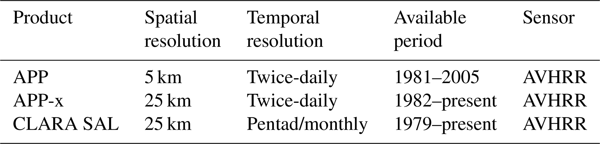
Early research estimated sea ice albedo through parameterization schemes. These schemes established empirical functions relating sea ice albedo to environmental parameters such as ice surface temperature, snow depth, and ice thickness, thus providing albedo values for different states of ice melt (Lynch et al., 1995; Parkinson and Washington, 1979; Ross and Walsh, 1987; Schramm et al., 1997). At present, satellite remote sensing is widely used for capturing key sea ice parameters on a large scale. Numerous studies utilize satellite data to calculate the sea ice albedo in the Arctic region and have published several products (Cheng et al., 2023; Key et al., 2001; Liang et al., 2013; Lindsay and Rothrock, 1994; Niehaus et al., 2024; Qu et al., 2016; Riihelä et al., 2013; Stroeve et al., 2005). However, products related to the Antarctic sea ice albedo are limited. The currently available long-time Antarctic sea ice albedo products are developed based on Advanced Very High-resolution Radiometer (AVHRR) data (Table 1), including the AVHRR Polar Pathfinder (APP) albedo product (Key et al., 2001), the APP-extended (APP-x) albedo product (Key et al., 2016; Wang and Key, 2005), and the Satellite Application Facility on Climate Monitoring (CM-SAF) cLouds, Albedo and RAdiation (CLARA) surface albedo (SAL) product (Karlsson et al., 2023b).

Table 1 Currently available broadband albedo products for Antarctic sea ice.

Although these products have been widely employed in Antarctic climate models and made significant progress, they require further improvements. First, they rely on narrow-to-broadband conversion of reflectance under a Lambertian surface assumption, which ignores the anisotropy of the sea ice surface (Karlsson et al., 2023a; Key et al., 2016; Zhou et al., 2023). However, the sea ice surface cannot be simply considered as Lambertian, as dry snow and ice surfaces have strong directional effects of forward scattering. Second, they only use the AVHRR channel 1 (0.55–0.90 µm) and channel 2 (0.725–1.10 µm) reflectance data in the process of narrow-to-broadband conversion, not covering the full shortwave range (Stroeve et al., 2005). Finally, the majority of Antarctic sea ice is seasonal ice and experiences frequent snowfall (Campagne et al., 2016; Winkelmann et al., 2012). As a result, these products may not be able to accurately depict the sea ice anisotropy and dynamic changes due to their relatively coarse spatiotemporal resolutions.

The Multiband Reflectance Iteration (MBRI) algorithm was proposed by our previous work (Cheng et al., 2023) to generate a daily 500 m Arctic sea ice albedo product. This algorithm takes full consideration of the inherent heterogeneity and anisotropy of the sea-ice physical and optical properties for the accurate calculations of Arctic sea-ice albedo from the Moderate Resolution Imaging Spectroradiometer (MODIS). However, the MODIS level-2 surface reflectance data does not cover the Antarctic marine regions. Then, this study used multi-band Visible Infrared Imaging Radiometer Suite (VIIRS) reflectance data with high quality and global coverage to generate Antarctic sea ice albedo product. We improve the MBRI algorithm, facilitating its applicability for VIIRS reflectance bands for sea ice albedo retrieval. The cloud-induced impacts on sea ice albedo are also corrected. Then we generate the first 1 km, seamless, daily Antarctic sea ice albedo product from 2012 to 2021 (hereafter referred to as the MBRI albedo product). Additionally, we performed an uncertainty analysis and a comprehensive accuracy assessment using in situ measurements and existing products.

This paper is organized as follows. Section 2 introduces the datasets used for the generation and validation of the proposed MBRI albedo product. Section 3 describes the methodology and processing steps. Section 4 presents the uncertainty analysis and validation results. Last, Sects. 5, 6 and 7 provide the discussion, data availability and key conclusions of this work, respectively.

2 Data

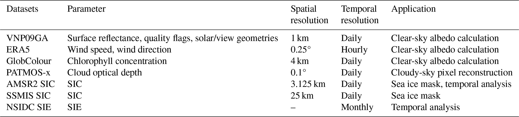
The generation of the MBRI albedo product utilized multiple satellite and reanalysis products. The data sources employed for clear-sky pixel albedo retrieval include: the VIIRS/NPP Surface Reflectance Daily L2G Global 1 km and 500 m SIN Grid (VNP09GA) product; the European Centre for Medium-Range Weather Forecasts (ECMWF) Reanalysis v.5 (ERA5) wind products; and the Global Ocean Colour (GlobColour) chlorophyll concentration product. Sea ice albedo under cloudy-sky was reconstructed based on the Pathfinder Atmospheres–Extended (PATMOS-x) cloud optical depth dataset. Sea ice pixels were identified using the Advanced Microwave Scanning Radiometer 2 (AMSR2) and Special Sensor Microwave Imager/Sounder (SSMIS) sea ice concentration (SIC) datasets. In addition, the MBRI albedo product were comprehensively assessed based on seven ground sites from the Baseline Surface Radiation Network (BSRN), the Institute for Marine and Atmospheric Research Utrecht (IMAU), and Alfred Wegener Institute (AWI) networks. Furthermore, the MBRI albedo product was compared with the APP-x and CLARA Edition 3 (CLARA-A3) products.

2.1 Satellite and reanalysis data

VNP09GA product is the primary source data for calculating Antarctic sea ice albedo under clear-sky conditions. Provided by the Level-1 and Atmosphere Archive & Distribution System Distributed Active Archive Center (LAADS DAAC), the VNP09GA product is available at https://ladsweb.modaps.eosdis.nasa.gov/missions-and-measurements/products/VNP09GA (last access: 21 September 2025, Vermote et al., 2023). Its M-band data provides daily 1 km surface reflectance in the shortwave spectrum. The product spans from 19 January 2012, to the present, and it adopts the Sinusoidal projection, gridded according the MODIS Sinusoidal Tile Grid.

The 10 m u-component (eastward) and v-component (northward) wind products from the ERA5 are used for the clear-sky albedo calculations. Compared to previous versions, ERA5 exhibits significant improvements in both spatial and temporal resolution, as well as overall accuracy (Dee et al., 2011; Hersbach et al., 2020). Hourly ERA5 data is available at https://doi.org/10.24381/cds.adbb2d47 (Hersbach et al., 2023).

The GlobColour project, initiated by the European Space Agency (ESA) and available at https://hermes.acri.fr/ (last access: 21 September 2025), provides a continuous dataset of merged L3 Ocean Colour products (Maritorena et al., 2010). We used the GlobColour chlorophyll concentration to participate in the calculation of clear-sky albedo.

The PATMOS-x cloud optical depth data was used to reconstruct the sea ice albedo for pixels missing due to cloud coverage. The PATMOS-x is provided by the National Oceanic and Atmospheric Administration (NOAA) and available at https://www.ncei.noaa.gov/metadata/geoportal/rest/metadata/item/gov.noaa.ncdc:C00926/html (last access: 21 September 2025, Foster et al., 2021). Compared to previous versions, PATMOS-x version 6.0 (Pv6.0) is more stable, with less inter-satellite variability, and provides a more consistent polar cloud detection, phase distribution, and cloud-top height distribution (Foster et al., 2023; Heidinger et al., 2014).

To identify the sea ice pixels, the AMSR2 SIC dataset (3.125 km resolution, provided by the University of Bremen) was used (Spreen et al., 2008). Additionally, the 25 km resolution SSMIS SIC dataset was selected to fill gaps in the AMSR2 SIC data (DiGirolamo et al., 2022). The two SIC datasets are available at https://seaice.unibremen.de/sea-ice-concentration/amsre-amsr2/ (last access: 21 September 2025) and https://nsidc.org/data/nsidc-0051/versions/2 (last access: 21 September 2025), respectively. Sea ice extent (SIE) data from the National Snow and Ice Data Center (NSIDC) (Fetterer et al., 2017), available at https://doi.org/10.7265/N5K072F8, was also employed to conduct a temporal analysis of the proposed albedo dataset.

Table 2 summarizes the information of satellite and reanalysis products used to generate MBRI albedo product in this study.

Table 2 Basic information of satellite and reanalysis products used to generate MBRI albedo product.

2.2 Comparative data

2.2.1 Existing Antarctic sea ice albedo products

This study uses two Antarctic sea ice albedo datasets as comparative data. One is APP-x, a thematic climate data record that contains 19 variables of the surface, cloud properties, and radiative fluxes (Key et al., 2016). APP-x albedo is generated based on AVHRR data, employing the Lambertian surface assumption. It is mapped to a 25 km EASE grid at 02:00 and 14:00 (local solar time) for the Antarctic region. The APP-x product is available at https://www.ncei.noaa.gov/products/climate-data-records/extended-avhrr-polar-pathfinder (last access: 21 September 2025, Key et al., 2019).

The other dataset is the CLARA-A3 SAL product, which provides radiation parameters and cloud properties, also based on AVHRR data. It includes black-sky, white-sky, and blue-sky surface albedos, presented as monthly and pentad (5 d) averages. It is provided on a 25 km resolution equal-area grid, covering the polar regions. The product accounts for anisotropic effects by averaging the directional sea ice reflectance over a specified period (5 d or more) (Karlsson et al., 2023a). The CLARA-A3 SAL product is available at https://wui.cmsaf.eu/safira/action/viewProduktDetails?eid=22564&fid=40 (last access: 21 September 2025).

2.2.2 In situ measurements

This study collected in situ measurement datasets from seven sites to evaluate the accuracy of the MBRI albedo product.

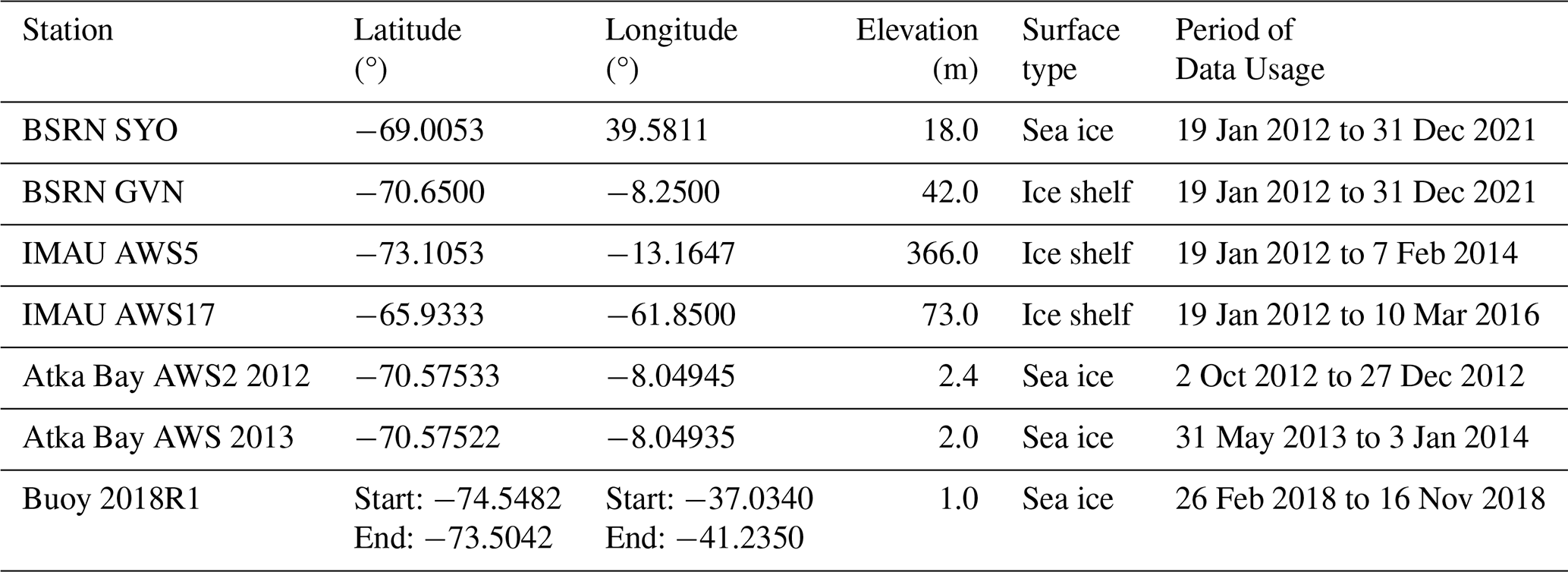
The World Climate Research Programme BSRN provides high-quality ground-based radiation measurements every minute since 1992. This study selects measurements from the SYO and GVN stations of the BSRN. The SYO station is located on East Ongul Island in East Antarctica, about 4 km from the continent, with sea ice as the observed surface type (Tanaka, 2022). The GVN station is located on the Ekström Ice Shelf, in the Atka Bay area of the northeastern Weddell Sea (König-Langlo and Loose, 2007). The measurements of BSRN is available at https://bsrn.awi.de/data/data-retrieval-via-pangaea/ (last access: 21 September 2025).

Since 1995, the IMAU at Utrecht University has deployed 19 AWSs in Antarctica, measuring a range of meteorological and atmospheric parameters. Considering the measured parameters and locations of the AWSs, this study selected data from AWS5 (two-hourly) and AWS17 (hourly) for validation. AWS5 is located on the Riiser-Larsen Ice Shelf, while AWS17 is situated on the remnants of the Larsen B Ice Shelf at Scar Inlet (Jakobs et al., 2020). Further data details can be found at https://doi.org/10.1594/PANGAEA.974080 (last access: 21 September 2025, van Tiggelen et al., 2025).

This study also collected measurement datasets from several AWSs deployed by the AWI, Helmholtz Centre for Polar and Marine Research. One dataset is from AWSs installed by Hoppmann et al. (2014, 2015a), located nearly at the same site on the Atka Bay land-fast sea ice (named Atka Bay AWS2 2012 and Atka Bay AWS 2013, 1 min interval). These stations recorded the transformation of a first-year fast ice in Atka Bay into thick second-year sea ice, which eventually disintegrated into small floes (Hoppmann et al., 2015b, c). Another dataset comes from the radiation station (named Buoy 2018R1, hourly) installed by Nicolaus et al. (2024) on a first-year ice in the Weddell Sea, which drifted with the coastal currents. These datasets are available at https://doi.org/10.1594/PANGAEA.824527 (Hoppmann et al., 2014), https://doi.org/10.1594/PANGAEA.833975 (Hoppmann et al., 2015a) and https://doi.org/10.1594/PANGAEA.949507 (Nicolaus et al., 2024), respectively.

The station locations are shown in Fig. 1, with further details provided in Table 3.

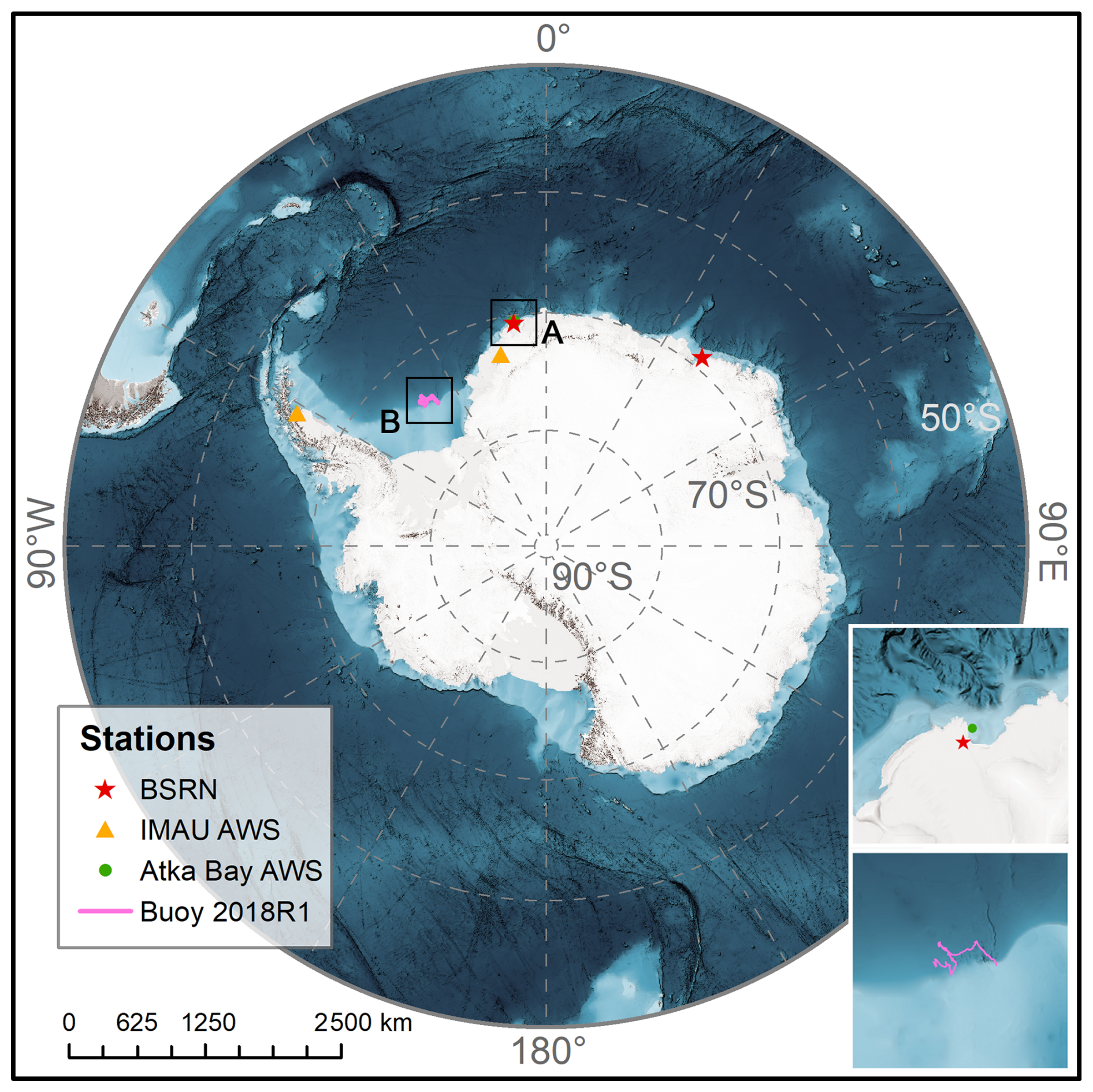
Figure 1 Distribution map of the in situ stations.

Table 3 Basic information of the in situ stations.

When preprocessing these in situ measurement datasets, except for Buoy 2018R1, which directly provides albedo values, the albedo values from other stations are derived from the ratio of shortwave upward to shortwave downward radiation. After filtering the data based on quality flags, daily albedo values are obtained by averaging the measurements taken near local solar noon. For the MBRI albedo product, in order to reduce geographic matching errors, the nearest pixel to each station is selected, and a 3 × 3 window average is used as the reference value for validation. Furthermore, when compared to APP-x product, the MBRI albedo product is resampled at a 25 km resolution, and when compared to CLARA-A3 product, the resampled MBRI albedo and in situ measurements are averaged over a 5 d period.

3 Methodology

3.1 Framework

The accurate inversion of surface albedo relies on the construction of the Bidirectional Reflectance Distribution Function (BRDF). The MBRI algorithm assumes the sea ice BRDF is a linear combination of the BRDFs associated with ocean water and snow/ice. Building upon the assumption, the sea ice BRDF is retrieved by an iterative process with single-angular/date multi-band reflectance data. The sea ice broadband albedo is subsequently estimated from multi-band satellite observations (Cheng et al., 2023). In contrast to conventional algorithms relying on multi-date/angular data, the MBRI algorithm enables the acquisition of albedo with finer temporal resolution and enhances the representation of rapid changes occurring on the sea ice surface.

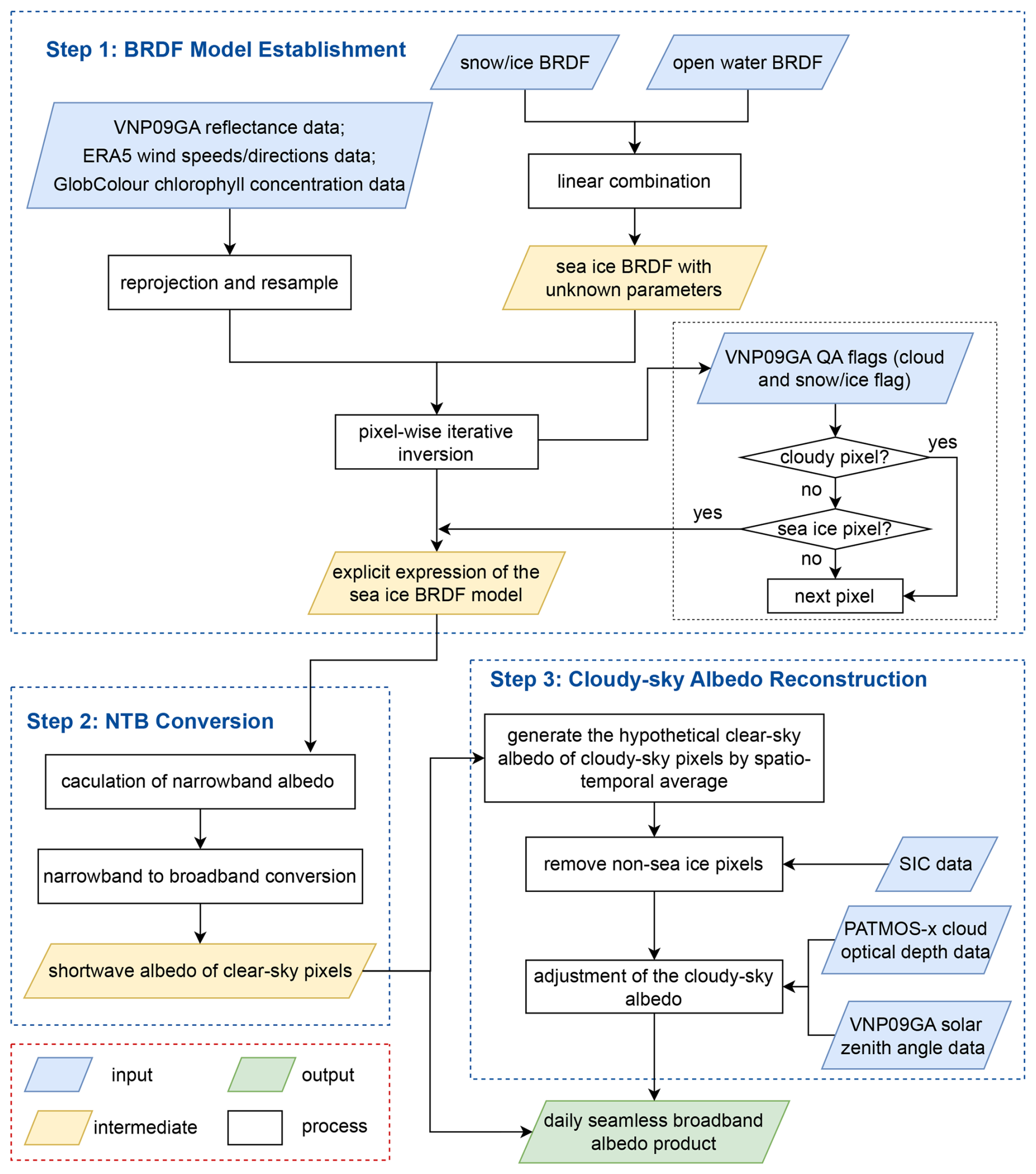
Figure 2 presents the flowchart for the generation of the MBRI albedo product. This method involves three key steps: (1) BRDF model establishment: The sea ice BRDF is constructed based on radiative transfer models and derived through an iterative process to express it explicitly. (2) Broadband albedo estimation: The narrowband albedo is estimated by integrating the derived sea ice BRDF over the angles of incidence and reflection, and the broadband albedo is then calculated by the narrowband to broadband (NTB) conversion. (3) Reconstruction of cloudy-sky albedo: The sea ice albedo of cloudy pixels is reconstructed by integrating spatiotemporal information and physical models. These steps are elaborated upon in the following subsections.

Figure 2 Flowchart for the generation of the proposed Antarctic sea ice albedo product.

3.2 Establishment and calculation of the sea ice BRDF model

3.2.1 Sea ice BRDF establishment

In polar regions, the sea ice cover is typically considered to comprise snow-covered ice, bare ice, melt ponds, and open water. At the scale of remote sensing satellite pixels, the reflectance of sea ice and melt ponds can be jointly determined by the reflectance of snow, ice, and ocean water. Consequently, its value can be approximated as a linear summation of these three components (Qu et al., 2016). Note that the determining factors for the optical parameters of bare ice closely are similar to those of snow (Kokhanovsky and Zege, 2004; Zege et al., 2015). Therefore, the MBRI algorithm considers ice and snow as a unified entity and employs a single model to describe their reflectance properties. Based on the above, the sea ice BRDF model can be expressed as (Cheng et al., 2023):

$$\begin{array}{}\text{(1)}& B_{\text{sea-ice}}=f_{\mathrm{s}}\cdot B_{\mathrm{snow}/\mathrm{ice}}+(\mathrm{1}-f_{\mathrm{s}})\cdot B_{\mathrm{ocean}},\end{array}$$

Where B_sea-ice, $B_{\mathrm{snow}/\mathrm{ice}}$, and B_ocean are the BRDF over the surfaces of sea ice, snow/ice, and ocean water, respectively; and f_s represents the fraction of snow/ice in a mixture of snow, ice, and seawater, where these components are blended in varying proportions.

Asymptotic Radiative Transfer (ART) model has been demonstrated to accurately characterize the reflectance properties over snow/ice surfaces (Zege et al., 2011). We employed this model for the BRDF of snow/ice surface as follows:

$$\begin{array}{}\text{(2)}& B_{\mathrm{snow}/\mathrm{ice}}\left({\mathit{\theta }}_{\mathrm{s}},{\mathit{\theta }}_{\mathrm{v}},\mathit{\phi }\right)=B_{\mathrm{0}}\left({\mathit{\theta }}_{\mathrm{s}},{\mathit{\theta }}_{\mathrm{v}},\mathit{\phi }\right)\exp \left[-t{\displaystyle \frac{g\left({\mathit{\theta }}_{\mathrm{s}}\right)g\left({\mathit{\theta }}_{\mathrm{v}}\right)}{B_{\mathrm{0}}\left({\mathit{\theta }}_{\mathrm{s}},{\mathit{\theta }}_{\mathrm{v}},\mathit{\phi }\right)}}\right],\end{array}$$

where θ_s, θ_v, and φ are the solar zenith angle (SZA), view zenith angle (VZA) and relative azimuth angle (RAA), respectively. $B_{\mathrm{0}}\left({\mathit{\theta }}_{\mathrm{s}},{\mathit{\theta }}_{\mathrm{v}},\mathit{\phi }\right)$ is the BRDF of the semi-infinite non-absorbing layer, which can be expressed as (Kokhanovsky et al., 2005):

$$\begin{array}{}\text{(3)}& \begin{array}{rl}& B_{\mathrm{0}}\left({\mathit{\theta }}_{\mathrm{s}},{\mathit{\theta }}_{\mathrm{v}},\mathit{\phi }\right)\\ & ={\displaystyle \frac{a+b\left(\cos {\mathit{\theta }}_{\mathrm{s}}+\cos {\mathit{\theta }}_{\mathrm{v}}\right)+c\cos {\mathit{\theta }}_{\mathrm{s}}\cos {\mathit{\theta }}_{\mathrm{v}}+p\left(\mathrm{\Theta }\right)}{\mathrm{4}\left(\cos {\mathit{\theta }}_{\mathrm{s}}+\cos {\mathit{\theta }}_{\mathrm{v}}\right)}},\end{array}\end{array}$$

where a= 1.247, b= 1.186, and c= 5.157; p(Θ) is the phase function; and Θ is the scattering angle (measured in degrees). The latter two can be parameterized as:

$$\begin{array}{}\text{(4)}& {\displaystyle }p\left(\mathrm{\Theta }\right)=\mathrm{11.1}\exp \left(-\mathrm{0.087}\mathrm{\Theta }\right)+\mathrm{1.1}\exp \left(-\mathrm{0.014}\mathrm{\Theta }\right),\text{(5)}& {\displaystyle }\mathrm{\Theta }=\arccos \left(-\cos {\mathit{\theta }}_{\mathrm{v}}\cos {\mathit{\theta }}_{\mathrm{s}}+\sin {\mathit{\theta }}_{\mathrm{v}}\sin {\mathit{\theta }}_{\mathrm{s}}\cos \mathit{\phi }\right).\end{array}$$

Zege et al. (2011) defined the escape function at zenith angle θ (g(θ)) and the fraction of the absorbed energy from a semi-infinite medium under diffuse illumination (t) in Eq. (2), as follows:

$$\begin{array}{}\text{(6)}& {\displaystyle }g\left(\mathit{\theta }\right)={\displaystyle \frac{\mathrm{3}}{\mathrm{7}}}\left(\mathrm{1}+\mathrm{2}\cos \mathit{\theta }\right),\text{(7)}& {\displaystyle }t=A\sqrt{{\displaystyle \frac{\mathrm{4}\mathit{\pi }}{\mathit{\lambda }}}{a}_{\mathrm{ef}}\left(\mathit{\chi }+C\right)},\end{array}$$

where λ represents wavelength; a_ef is the snow/ice effective grain size; C is a parameter representing the absorption capacity at wavelength λ of soot pollutants in snow, determined by its relative concentration; A is a parameter representing the particle's shape, taking a value of 5.8 in this study; and χ is the imaginary part of the complex refractive index of snow/ice, with values for different wavelengths obtained online at http://www.atmos.washington.edu/ice_optical_constants (last access: 21 September 2025, Warren and Brandt, 2008).

If the values of the wavelength-independent unknown variables a_ef and C are determined, then the reflectance of snow/ice surfaces in any incident and reflection direction at a specified wavelength can be represented by Eq. (2).

In addition, the BRDF over the ocean water surface is derived using the three-component ocean water albedo (TCOWA) model proposed by Feng et al. (2016), as follows:

$$\begin{array}{}\text{(8)}& B_{\mathrm{ocean}}=f_{\mathrm{w}}\cdot B_{\mathrm{wc}}+\left(\mathrm{1}-f_{\mathrm{w}}\right)\cdot \left(B_{\mathrm{g}}+B_{\mathrm{wl}}\right),\end{array}$$

where B_wc, B_g, and B_wl are the BRDFs of whitecaps, sun glint, and water-leaving, respectively; f_w is the coverage of whitecaps. According to previous studies, the four components can be explicitly expressed as functions of chlorophyll concentration, wind speed/direction, wavelength, and solar/view geometries (Callaghan et al., 2008; Cox and Munk, 1954; Feng et al., 2016; Morel et al., 2002; Wang et al., 2023).

3.2.2 Sea ice BRDF model calculation

Equations (2)–(8) indicate that three unknown parameters still exist in the established sea ice BRDF model: soot pollutant relative concentration C; fraction of snow/ice f_s; and snow/ice effective grain size a_ef. To simplify the representation, we define vector $\mathit{X}=\left(a_{\mathrm{ef}},C,f_{\mathrm{s}}\right)$. These three parameters are inherent properties of sea ice and are wavelength-independent. Therefore, if there are three or more observational values at different wavelengths, an inversion method can be employed to calculate them.

In this paper, considering that the absorption spectrums of soot pollutants and snow/ice grain are mainly in the visible and near-infrared bands, respectively (Zege et al., 2011), we utilized the reflectance data from VIIRS channels 3 (490 nm), 7 (865 nm), and 8 (1240 nm), and solar/view geometries as the observational values. As Eq. (1) is nonlinear, the Newton–Raphson iteration method (Winkler, 1993) is employed to calculate the three unknown parameters for each pixel. In the iteration procedure, we take the natural logarithm of the three unknown parameters to reduce the impact of significant differences in their magnitudes on the calculation. Matrix M, representing the derivatives of B_sea-ice with respect to each component of vector X, is then computed as:

$$\begin{array}{}\text{(9)}& \begin{array}{rl}\mathbf{M}& =\left(M_{ik}\right)\\ & =\left({\displaystyle \frac{\partial B_{\text{sea-ice}}^i}{\partial \ln X_k}}\right)=\left(\begin{array}{ccc}\frac{\partial B_{\text{sea-ice}}^{\mathrm{3}}}{\partial \ln a_{\mathrm{ef}}}& \frac{\partial B_{\text{sea-ice}}^{\mathrm{7}}}{\partial \ln a_{\mathrm{ef}}}& \frac{\partial B_{\text{sea-ice}}^{\mathrm{8}}}{\partial \ln a_{\mathrm{ef}}}\\ \frac{\partial B_{\text{sea-ice}}^{\mathrm{3}}}{\partial \ln C}& \frac{\partial B_{\text{sea-ice}}^{\mathrm{7}}}{\partial \ln C}& \frac{\partial B_{\text{sea-ice}}^{\mathrm{8}}}{\partial \ln C}\\ \frac{\partial B_{\text{sea-ice}}^{\mathrm{3}}}{\partial \ln f_{\mathrm{S}}}& \frac{\partial B_{\text{sea-ice}}^{\mathrm{7}}}{\partial \ln f_{\mathrm{S}}}& \frac{\partial B_{\text{sea-ice}}^{\mathrm{8}}}{\partial \ln f_{\mathrm{S}}}\end{array}\right),\end{array}\end{array}$$

where X_k is the kth component of X. According to studies on snow/ice physical parameters (Dang et al., 2015; Yang et al., 2017; Zege et al., 2015), X can be initialized with the values a_ef=300 µm, $C=\mathrm{2}\times {\mathrm{10}}^{-\mathrm{6}}$ and f_s=0.5, representing the initial state. $B_{\text{sea-ice}}^i$ is the BRDF in the ith channel (i= 3, 7, 8), which can be interpreted as the reflectance in the ith channel, calculated using Eq. (1) at specific viewing and solar angles.

Following this, vector X is updated using the correction ΔX_k as follows:

$$\begin{array}{}\text{(10)}& {\displaystyle }\mathrm{\Delta }{X}_k=\left(\mathit{B}-{\mathit{B}}^n\right){\mathbf{M}}^{-\mathrm{1}},\text{(11)}& {\displaystyle }{X}_k^{n+\mathrm{1}}=X_k^n\exp \left(\mathrm{\Delta }{X}_k\right),\end{array}$$

where n is the nth iteration; B=(Bⁱ) is the vector composed of the observed reflectance of the VIIRS ith channel; and Bⁿ is the vector of $B_{\text{sea-ice}}^i$ on the nth iteration step. The nonlinearity of Eq. (9) ensures that matrix M does not exhibit linear dependence. Therefore, the result obtained from the iterative procedure is a non-singular solution. The iteration loop breaks when:

$$\begin{array}{}\text{(12)}& max\left(\mathrm{\Delta }{X}_k\right)<\mathrm{0.001},\end{array}$$

and typically converges after three to four iterations.

3.3 Broadband albedo estimation

The black-sky albedo, also denoted as directional-hemispherical reflectance, is defined as the albedo of a surface under radiation from a single direction and without atmospheric scattering. It can be expressed as the integration of the BRDF over the viewing semi-hemisphere as follows (Schaepman-Strub et al., 2006):

$$\begin{array}{}\text{(13)}& {\mathit{\alpha }}_{\mathrm{bsa}}={\int }_{\mathrm{0}}^{\mathrm{2}\mathit{\pi }}{\int }_{\mathrm{0}}^{\mathit{\pi }/\mathrm{2}}{B}_{\text{sea-ice}}\left({\mathit{\theta }}_{\mathrm{s}},{\mathit{\theta }}_{\mathrm{v}},{\mathit{\phi }}_{\mathrm{s}},{\mathit{\phi }}_{\mathrm{v}}\right)\cos {\mathit{\theta }}_{\mathrm{v}}\sin {\mathit{\theta }}_{\mathrm{v}}\mathrm{d}{\mathit{\theta }}_{\mathrm{v}}\mathrm{d}{\mathit{\phi }}_{\mathrm{v}},\end{array}$$

where α_bsa is the black-sky albedo for each band; φ_s and φ_v is the solar and view azimuth angles, respectively.

Under ideal isotropic diffuse radiation, the surface albedo is referred to as white-sky albedo or bi-hemispherical albedo (Qu et al., 2015). The white-sky albedo (α_wsa) is obtained through further integration over all solar incident angles:

$$\begin{array}{}\text{(14)}& {\mathit{\alpha }}_{\mathrm{wsa}}={\int }_{\mathrm{0}}^{\mathrm{2}\mathit{\pi }}{\int }_{\mathrm{0}}^{\mathit{\pi }/\mathrm{2}}{\mathit{\alpha }}_{\mathrm{bsa}}\cos {\mathit{\theta }}_{\mathrm{s}}\sin {\mathit{\theta }}_{\mathrm{s}}\mathrm{d}{\mathit{\theta }}_{\mathrm{s}}\mathrm{d}{\mathit{\phi }}_{\mathrm{s}}.\end{array}$$

Natural daylight irradiation lies between complete direct illumination and complete scattering. Consequently, the blue-sky albedo, representing the true surface albedo, can be obtained by combining the black-sky albedo and white-sky albedo with appropriate weighting (Pinty et al., 2005; Qu et al., 2015):

$$\begin{array}{}\text{(15)}& {\mathit{\alpha }}_{\mathrm{blue}}=\left(\mathrm{1}-\mathit{\gamma }\right)\cdot {\mathit{\alpha }}_{\mathrm{bsa}}+\mathit{\gamma }\cdot {\mathit{\alpha }}_{\mathrm{wsa}},\end{array}$$

where α_blue is the blue-sky albedo; and γ is the diffuse skylight fraction. Under clear-sky conditions, γ can be empirically calculated as follows (Qu et al., 2016):

$$\begin{array}{}\text{(16)}& \mathit{\gamma }=\mathrm{0.122}+\mathrm{0.85}\exp \left(-\mathrm{4.8}\cos \left({\mathit{\theta }}_{\mathrm{s}}\right)\right),\end{array}$$

where θ_s is SZA.

The broadband surface albedo is obtained through linearly weighted calculations of narrowband albedo (Liang, 2001). In this study, we adopt the narrow-to-broadband conversion coefficients as follows (Liu et al., 2017):

$$\begin{array}{}\text{(17)}& \begin{array}{rl}\mathit{\alpha }& =\mathrm{0.2892}{\mathit{\alpha }}_{\mathrm{1}}-\mathrm{0.4141}{\mathit{\alpha }}_{\mathrm{2}}+\mathrm{0.6996}{\mathit{\alpha }}_{\mathrm{3}}+\mathrm{0.2738}{\mathit{\alpha }}_{\mathrm{7}}\\ & +\mathrm{0.1463}{\mathit{\alpha }}_{\mathrm{8}}-\mathrm{0.0309}{\mathit{\alpha }}_{\mathrm{10}},\end{array}\end{array}$$

where α is the broadband albedo covering the shortwave spectral range; α_i is the narrowband blue-sky albedo for VIIRS spectral channel i (specifically $i=\mathrm{1},\mathrm{2},\mathrm{3},\mathrm{7},\mathrm{8},\mathrm{10}$).

3.4 Reconstruction of sea ice albedo under cloudy-sky

In the Antarctic sea ice regions, where continuous cloud coverage reaches 60 %–90 %, substantial missing data exists in the albedo product estimated from VIIRS. Cloud radiative forcing has a notable impact on the albedo of snow/ice surfaces (Key et al., 2001; Stapf et al., 2020). To accurately express the cloudy-sky sea ice albedo, and to enhance the spatiotemporal continuity, this study combines spatiotemporal and physical modeling to reconstruct sea ice albedo under cloudy-sky conditions

First, a spatiotemporal averaging interpolation method is used to obtain the initial reference albedo for cloudy pixels as follows:

$$\begin{array}{}\text{(18)}& {\widehat{\mathit{\alpha }}}^j\left(x,y\right)={\displaystyle \frac{\sum _{\left(x_i,y_i\right)\in \mathrm{\Omega }}{\mathit{\alpha }}^j\left(x_i,y_i\right)}{m}},\end{array}$$

where $\widehat{\mathit{\alpha }}\left(x,y\right)$ is the initial reference albedo for the target pixel (x,y); Ω is the neighborhood 3 × 3 × 3 window of the target pixel. For each pixel i within Ω, α(x_i,y_i) represents its albedo. Additionally, m is the total number of other valid pixels in Ω, respectively; This calculation is iterated 10 times to ensure the filling of nearly all cloud pixels. j is the number of iterations in the loop.

Assuming a cloudy pixel's initial reference albedo annual time series is denoted as y_t, we employ the Whittaker smoother (Eilers, 2003) to denoise and fit series z, which is regarded as the hypothetical clear-sky albedo, as follows:

$$\begin{array}{}\text{(19)}& z={\left(\mathbf{I}+\mathit{\rho }{D}^{\prime }\mathbf{D}\right)}^{-\mathrm{1}}\mathbf{I}{y}_t,\end{array}$$

where I is a diagonal weight matrix, with 0 assigned for missing data and 1 otherwise; D is the first-order difference matrix of the identity matrix; and ρ is the smoothing parameter and controls the smoothness of z. Ye et al. (2023) determined ρ=5 yielded the optimal overall performance in reconstructing the albedo of the Greenland Ice Sheet.

Following this, we estimate the cloudy-sky albedo based on the hypothetical clear-sky albedo as follows (Key et al., 2001):

$$\begin{array}{}\text{(20)}& {\mathit{\alpha }}_{\mathrm{rec}}={\mathit{\beta }}_{\mathrm{1}}+{\mathit{\beta }}_{\mathrm{2}}{\mathit{\alpha }}_{\mathrm{hyp}}+{\mathit{\beta }}_{\mathrm{3}}\ln \left(\mathit{\tau }+\mathrm{1}\right)+{\mathit{\beta }}_{\mathrm{4}}\cos {\mathit{\theta }}_{\mathrm{s}},\end{array}$$

where α_rec and α_hyp represent the reconstructed cloudy-sky albedo and hypothetical clear-sky albedo, respectively; τ is the cloud optical depth; θ_s is SZA; ${\mathit{\beta }}_i\left(i=\mathrm{1},\mathrm{2},\mathrm{3},\mathrm{4}\right)$ are empirical coefficients with values of −0.0491, 1.07, 0.0217, and 0.0180 respectively, derived from Key et al. (2001) and rounded to 3 significant digits according to empirical coefficient conventions.

The steps outlined above encompass the comprehensive process of generating the daily 1 km seamless Antarctic sea ice albedo product.

3.5 Estimation of sea ice albedo uncertainty

As previously mentioned, the MBRI albedo production involves two main steps: broadband clear-sky albedo retrieval and cloudy-sky albedo reconstruction. This study separately quantifies uncertainty propagation in both processes.

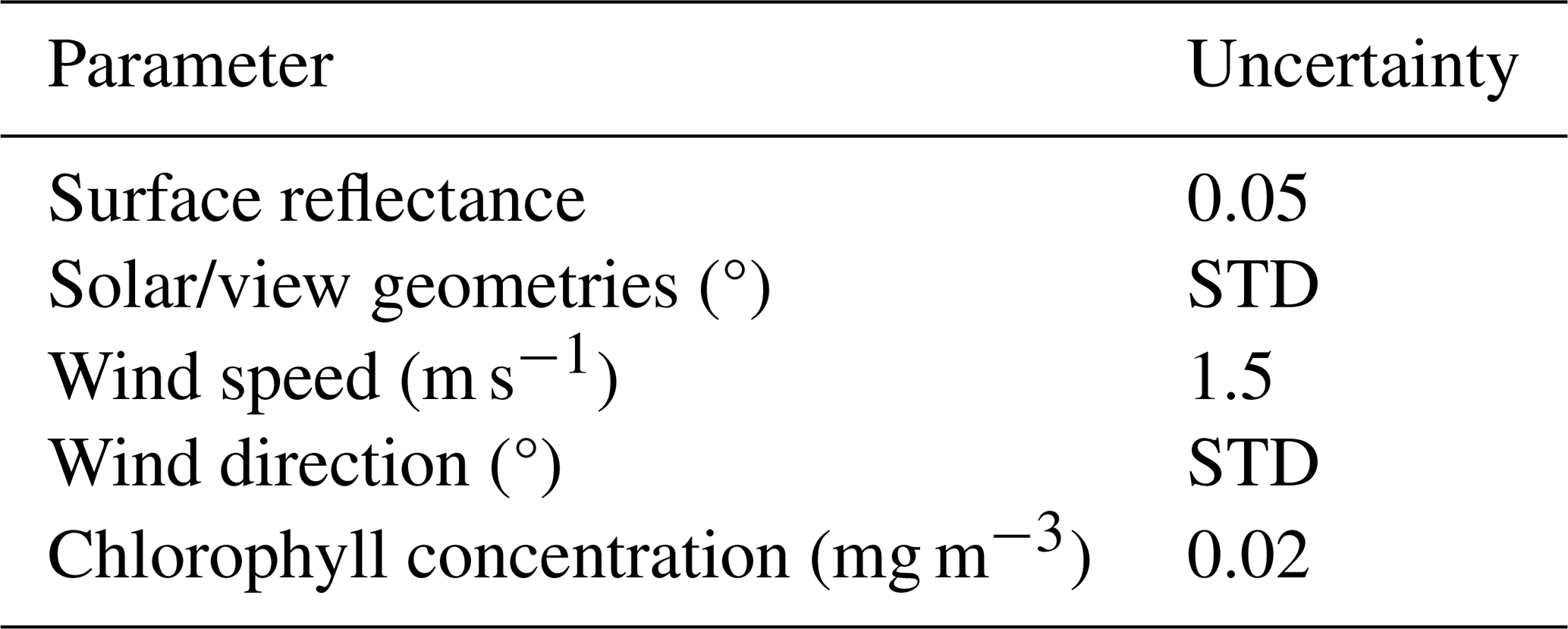
For the clear-sky albedo retrieval, the complex model employed here involves mathematical operations such as derivation and integration, making it difficult to derive the Gaussian error propagation formula. Therefore, the Monte Carlo method was used to assess the retrieval uncertainty (Mears et al., 2011; Zhou et al., 2018). First, each input parameter for 2012–2021 was divided into four seasons (spring: October–December, summer: January–March, autumn: April–June, and winter: July–September), and the ten-year mean for each parameter was calculated. The uncertainty for each parameter was referenced from the settings in previous studies or the validation accuracy (Jourdier, 2020; León-Tavares et al., 2024; Saulquin et al., 2019), as shown in Table 4. Notably, some angular data did not provide uncertainty, so the standard deviation (STD) of the mean was used as a substitute. Next, for each pixel, samples were drawn from the range of μ_i±σ_i (where μ_i is the mean and σ_i is the uncertainty for each parameter, with a sample size of 100 to balance computational efficiency and result stability). Finally, the albedo results for each pixel were obtained by inputting the samples into the retrieval model, with the standard deviation of these results representing the uncertainty for that clear-sky pixel. Then, in the MBRI albedo uncertainty dataset, the uncertainty for clear-sky pixels was determined based on the seasonal mean retrieval uncertainties.

Table 4 Uncertainties of input parameters. STD is the standard deviation of each input angle.

The reconstructed cloudy-sky albedo uncertainty primarily stems from the propagation of clear-sky albedo retrieval uncertainty, interpolation errors, and errors in cloud radiative forcing adjustment. According to Gaussian error propagation, the relationship can be expressed as:

$$\begin{array}{}\text{(21)}& {\mathit{\sigma }}_{\mathrm{cld}}^{\mathrm{2}}={\mathit{\sigma }}_{\mathrm{clr}}^{\mathrm{2}}+{\mathit{\sigma }}_{\mathrm{rec}}^{\mathrm{2}},\end{array}$$

where σ_cld represents the uncertainty of cloudy-sky albedo; σ_clr is the retrieval uncertainty of clear-sky albedo; σ_rec denotes the uncertainty introduced by the reconstruction process.

Equations (18)–(20) correspond to the key steps in the reconstruction of cloudy-sky albedo: interpolation of adjacent clear-sky pixels, temporal smoothing, and cloud radiative forcing correction. To simplify the uncertainty estimation, we treat interpolation and smoothing as a whole process and assume that errors from satellite angles are negligible. Based on Eq. (20), we derive the following relationship:

$$\begin{array}{}\text{(22)}& \begin{array}{rl}{\mathit{\sigma }}_{\mathrm{rec}}^{\mathrm{2}}& ={\left({\displaystyle \frac{\partial {\mathit{\alpha }}_{\mathrm{rec}}}{\partial {\mathit{\alpha }}_{\mathrm{hyp}}}}\cdot {\mathit{\sigma }}_{\mathrm{hyp}}\right)}^{\mathrm{2}}+{\left({\displaystyle \frac{\partial {\mathit{\alpha }}_{\mathrm{rec}}}{\partial \mathit{\tau }}}\cdot {\mathit{\sigma }}_{\mathit{\tau }}\right)}^{\mathrm{2}}\\ & ={\left({\mathit{\beta }}_{\mathrm{2}}\cdot {\mathit{\sigma }}_{\mathrm{hyp}}\right)}^{\mathrm{2}}+{\left({\displaystyle \frac{{\mathit{\beta }}_{\mathrm{3}}}{\mathit{\tau }+\mathrm{1}}}\cdot {\mathit{\sigma }}_{\mathit{\tau }}\right)}^{\mathrm{2}},\end{array}\end{array}$$

where σ_hyp is the uncertainty from the interpolation and smoothing process; σ_τ is the cloud optical depth uncertainty. Based on previous studies (Walther and Heidinger, 2012), the error in PATMOS-x cloud optical thickness can reach 20 %, so ${\mathit{\sigma }}_{\mathit{\tau }}=\mathit{\tau }\cdot \mathrm{0.2}$.

To estimate σ_hyp, we randomly masked some clear-sky pixels (over 400 000) and then reconstructed their albedo using interpolation and smoothing following Eqs. (18) and (19). Then, the cloudy-sky albedo uncertainty was calculated using Eqs. (21) and (22).

4 Results

4.1 Uncertainty analysis

4.1.1 Uncertainty of clear-sky albedo retrieval

Figure 3 shows the spatial distribution of clear-sky albedo retrieval uncertainty for the four seasons. The average uncertainties for spring and summer are approximately 0.030 and 0.029, respectively, higher than the 0.015 and 0.016 observed in autumn and winter. In autumn and winter, over 90 % of pixels have uncertainties less than 0.02. The annual average sea ice albedo uncertainty is 0.022. Spatially, uncertainty is relatively higher in the marginal ice zone and coastline, while it is lower in stable pack ice areas. This may due to the stronger influence of open water and ocean currents in these regions, leading to more significant changes in sea ice conditions, particularly in spring and summer, resulting in higher uncertainty in albedo retrieval.

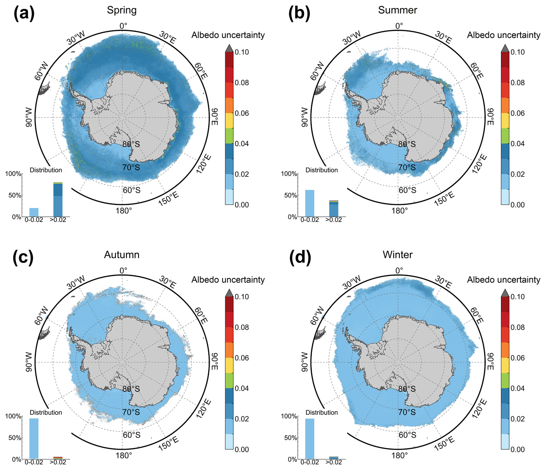
Figure 3 Spatial distribution of clear-sky retrieval albedo uncertainty for the four seasons. The histogram in the lower-left corner of each subplot shows the proportion of pixels with uncertainty less than 0.02 and greater than 0.02.

Due to the anisotropy of sea ice surfaces, clear-sky albedo retrieval exhibits significant sensitivity to solar/view geometries. To assess the relationship between retrieval uncertainty and these angular conditions, we sampled the retrieval uncertainty results for all pixels across the four seasons based on the angle distribution proportions (sample size = 50 000). Kernel Density Estimation (KDE) was then applied to obtain the distributions of sample uncertainty with respect to SZA and VZA, as well as their correlation. Figure 4a shows the KDE distribution of albedo uncertainty with respect to SZA. Around 60° SZA, a relatively high uncertainty (up to approximately 0.045) is observed for more sample pixels, and decreases with increasing SZA (slope = −0.0005, p<0.01). Fig. 4b shows that the uncertainty is less sensitive to changes in the VZA (slope = 0.0001, p<0.01). It should be noted that some angles have a small proportion, which may not be well represented in the KDE distribution and correlation statistics. Therefore, based on the results in Fig. 4a, two SZA ranges were selected for further analysis: range 1 (55–65°), where uncertainty is relatively higher (representing ∼ 28.3 % of samples), and range 2 (75–85°), where the SZA is more concentrated (representing ∼ 47.6% of samples). The VZA (0–71°) and RAA (0–360°) were divided into angular bins with intervals of 2.5 and 5°, respectively. Then, the average uncertainty of each angular bin for range 1 and range 2 was calculated, as shown in Fig. 5. In SZA range 1 (Fig. 5a), uncertainty remains below 0.02 for most angular bins. For VZA less than 40°, uncertainty shows a slight increase across almost all RAA directions but generally stays below 0.03. However, when VZA exceeds 40°, uncertainty increases significantly (exceeding 0.1) in the backward scattering direction (RAA = 0° ± 30°). In SZA range 2 (Fig. 5b), uncertainty similarly remains mostly below 0.02, with significant increases again in the backward scattering direction for VZA greater than 40°. Additionally, isolated instances of higher uncertainty appear in other RAA directions, which indicates the need for an optimization algorithm specifically designed for large SZA. And such optimization is necessary because satellite observations typically are less reliable under large SZA conditions due to low solar radiation or obscure of clouds. Furthermore, a slight increase in uncertainty is observed around RAA = 65° and 245, although it remains within acceptable limits. The large uncertainties in the backward directions likely stem from the strong forward-scattering characteristics of the sea ice surface, making the model more sensitive to changes in the backward azimuth angle. However, according to the histogram in Fig. 3, these anomalous angles account for only a small fraction of the total albedo retrieval.

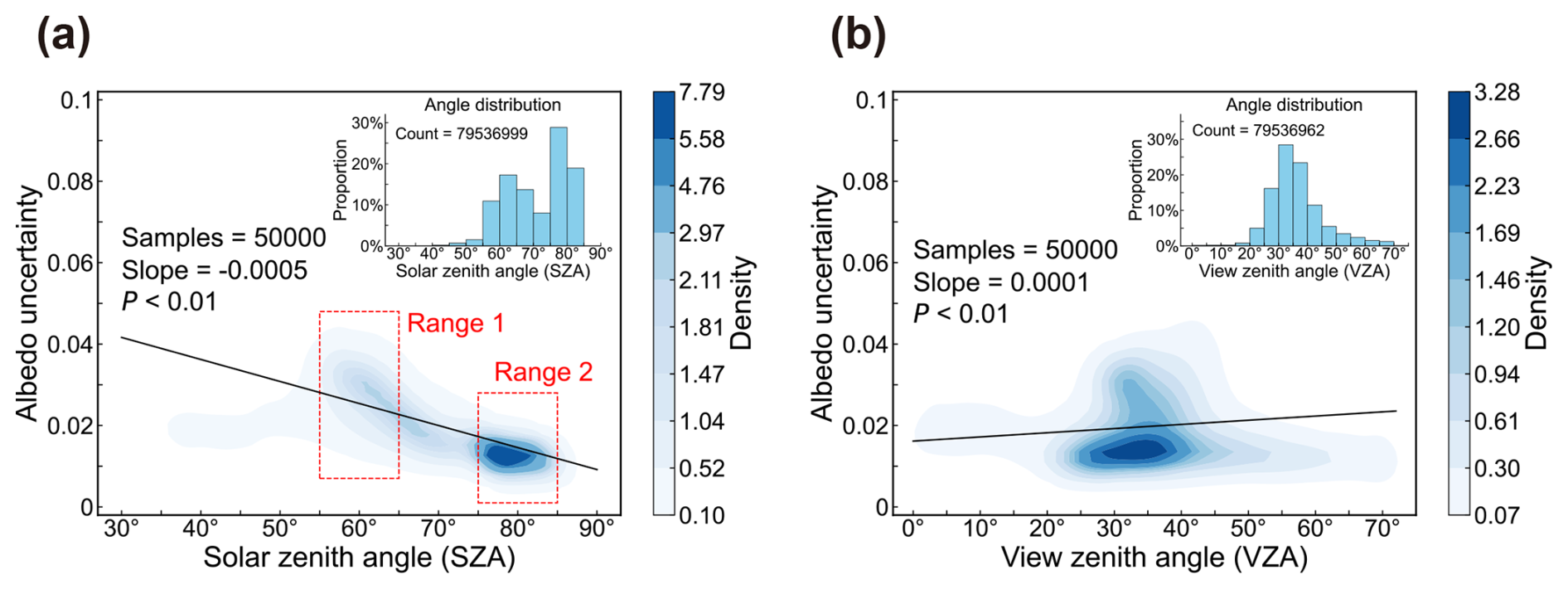
Figure 4 Kernel Density Estimation (KDE) plots of the uncertainty in sea ice albedo retrieval as a function of (a) solar zenith angle (SZA) and (b) satellite zenith angle (VZA). The histograms in the upper-right corners of each subplot represent the angular distributions. The black solid line denotes the fit line, while the red boxes in (a) indicate the two selected SZA ranges.

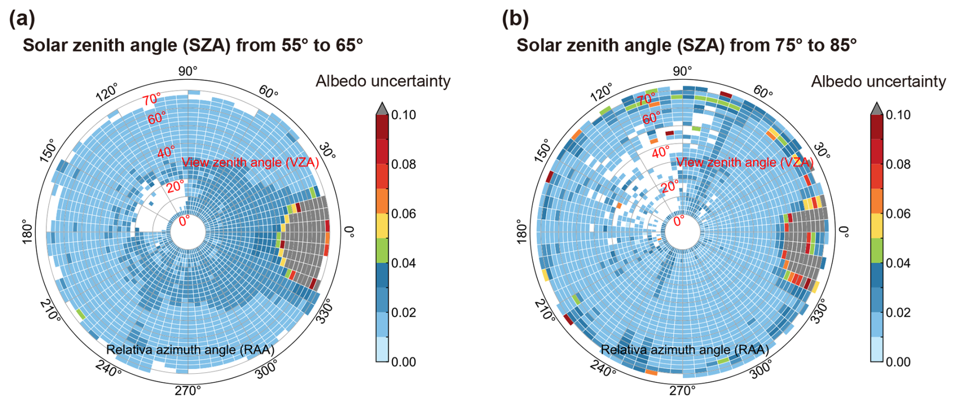
Figure 5 Angular distribution of the mean uncertainty in sea ice albedo retrieval. (a) Solar zenith angle from 55 to 65°; (b) Solar zenith angle from 75 to 85°. In the polar coordinate system, the radial direction represents the view zenith angle (from 0 to 71°), the angle direction represents the relative azimuth angle (from 0 to 360°). Blank areas indicate the absence of data for those angular bins in the sample.

4.1.2 Uncertainty of cloudy-sky albedo reconstruction

Figure 6a presents a scatter plot comparing the hypothetical albedo with the original clear-sky albedo, showing a correlation (R= 0.85) and a root mean square error (RMSE) of 0.065. Additionally, we analyzed the distribution of differences with respect to day of the year (DOY) and latitude (Fig. 6b and c). The differences exhibit a generally uniform horizontal distribution, indicating that interpolation and smoothing errors have no significant dependency on time or latitude. Therefore, we set σ_hyp=0.065, while σ_rec can be derived from the cloud optical depth data using Eq. (22). Finally, we can obtain the pixel-by-pixel cloud-sky albedo uncertainty from Eq. (21).

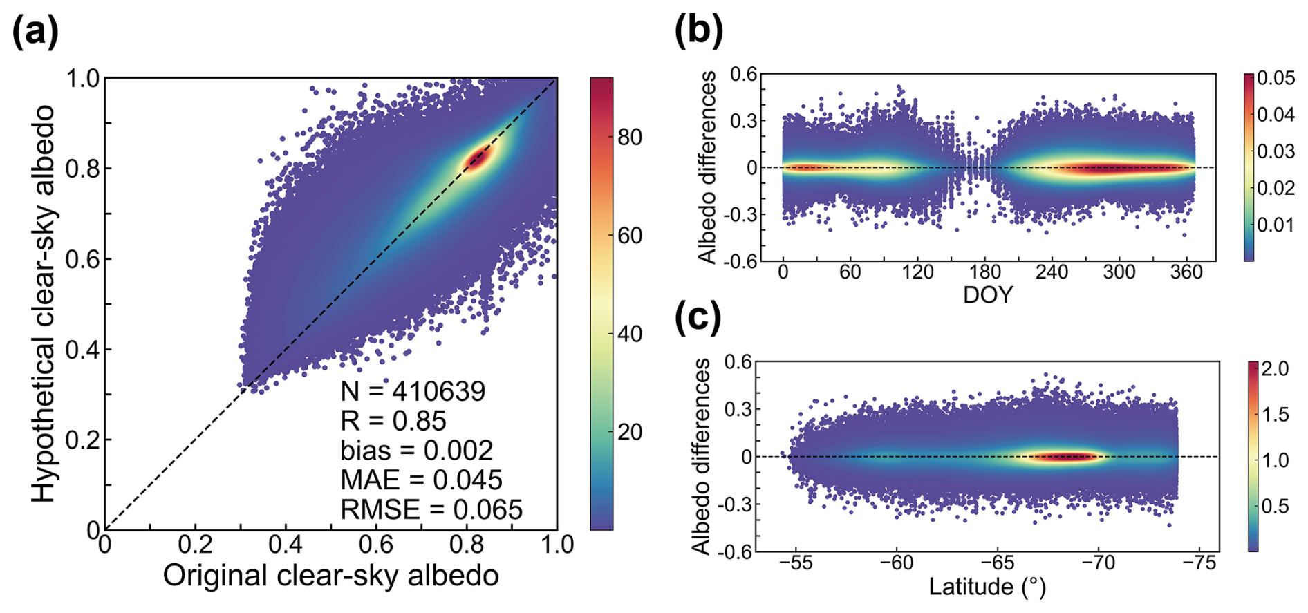
Figure 6 (a) Scatter plot of original albedo versus hypothetical albedo for the masked clear-sky pixels. Distribution of albedo differences with (b) DOY and (c) latitude.

4.2 Validation with in situ measurements

Figure 7 shows scatter plots comparing in situ measurements with three estimated albedo products. The RMSE for the original resolution MBRI albedo product and BSRN (including GVN and SYO stations) measurements is 0.071, with a correlation coefficient of 0.67 (Fig. 7a). After resampling the MBRI product to a 25 km resolution, the RMSE decreases to 0.064, while the RMSE for the APP-x product is 0.134 (Fig. 7b). The RMSE for the MBRI product further decreases to 0.054 after averaging over 5 d, while the corresponding RMSE for the CLARA-A3 product is 0.071 (Fig. 7c). Additionally, the MBRI product demonstrates the best correlation with the in situ measurements.

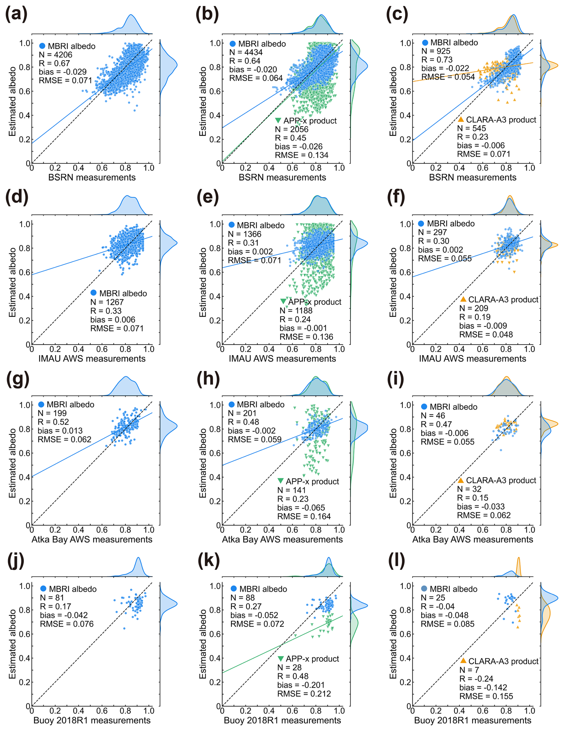
Figure 7 Scatter plots comparing the estimated albedo products with in situ measurements. (a)–(c) compare with BSRN measurements; (d)–(f) compare with IMAU AWS measurements; (g)–(i) compare with Atka Bay AWS measurements; (j)–(l) compare with Buoy 2018R1 measurements. Blue dots represent the MBRI albedo product; green inverted triangles represent the APP-x product; yellow triangles represent the CLARA-A3 product. The black dashed line represents the 1:1 line, and the solid line represents the fitted line (p-value < 0.01). N represents the number of comparisons, R represents the correlation coefficient, bias represents the mean difference error, and RMSE is the root mean square error.

When compared to IMAU AWS measurements (including AWS5 and AWS17) (Fig. 7d–f), the RMSE for the MBRI product is 0.071, unchanged after resampling to 25 km, and decreased to 0.055 after 5 d of averaging. The RMSE for the other two products is 0.136 and 0.048, respectively. Since AWS5 and AWS17 are located on more stable ice shelves, where albedo measurements exhibit smaller seasonal variations, the scatter plots show a more clustered distribution (Jakobs et al., 2020; Stroeve et al., 2005). Therefore, although the correlation coefficients are generally lower, the MBRI product still provides the best performance.

Among the Atka Bay AWSs, the MBRI albedo product also shows the best accuracy (Fig. 7g–i), with RMSE values of 0.062, 0.059, and 0.055 for the original, 25 km resampled, and 5-day averaged albedo, respectively. The corresponding RMSE for the APP-x and CLARA-A3 products are 0.164 and 0.062, respectively. Although the number of measurements for Buoy 2018R1 is limited, the MBRI product still demonstrates the smallest RMSE: 0.076, 0.072, and 0.085 (Fig. 7j–l). In contrast, the other two products show relatively poorer performance.

This section summarizes the validation results between the MBRI albedo product and in situ measurements from all stations, as shown in Fig. 8. Overall, the MBRI albedo product exhibits a good agreement with the ground truth values (R= 0.60), with an RMSE of 0.071 and a bias of −0.02. The slight underestimation of the MBRI albedo may be due to the broader spatial coverage of satellite observations compared to AWS. When sea ice further from the AWS begins to melt, AWS sensors only capture the albedo of ice and snow, while satellite pixels represent a mixture of snow/ice, melt ponds, and open water, leading to an underestimation of the albedo (Stroeve et al., 2005).

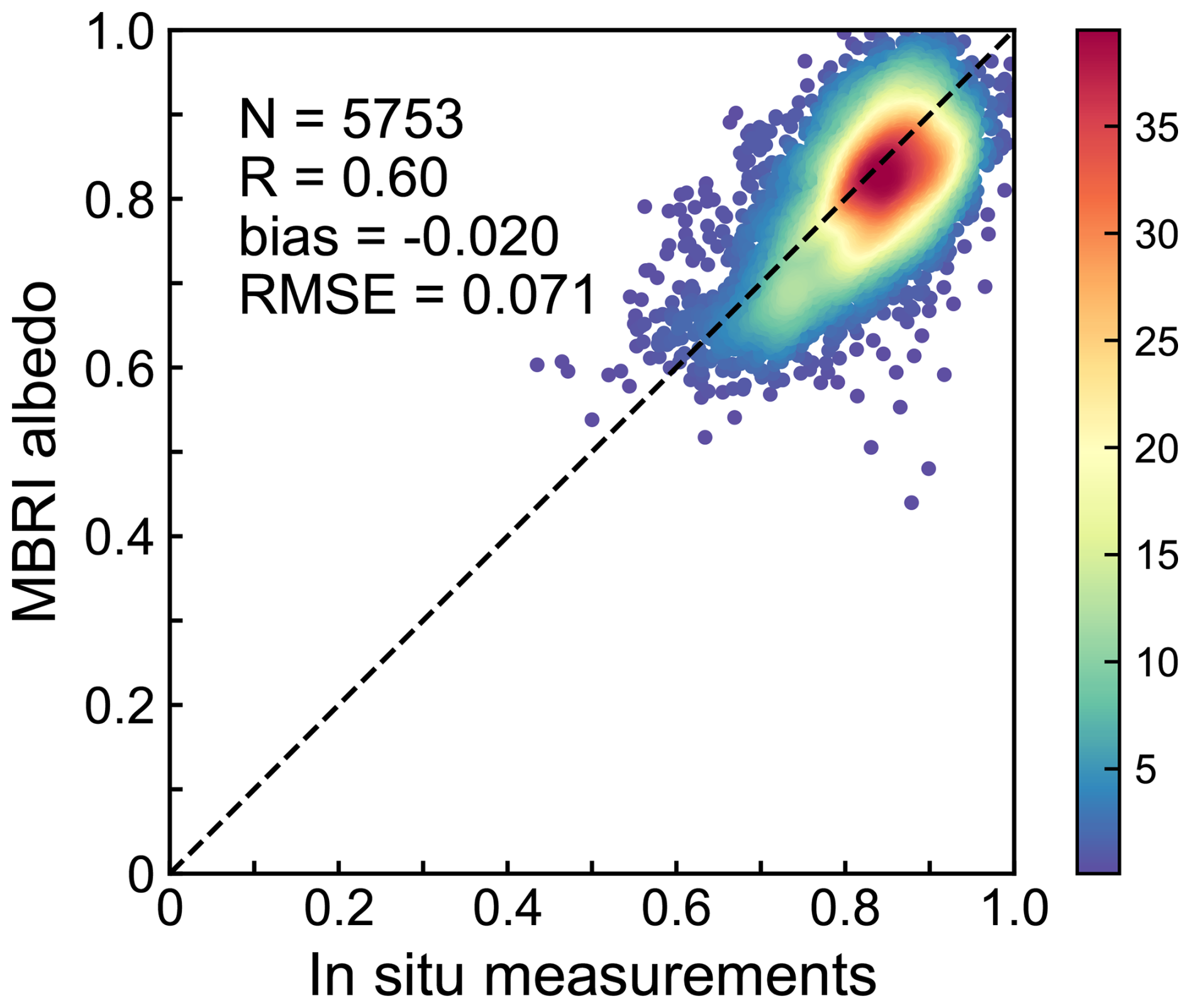
Figure 8 Probability density scatter plot of the MBRI albedo product compared to all in situ measurements.

4.3 Bias characteristics analysis and representative time series comparison

Figure 9 shows the distribution histogram of the bias (estimated albedo minus in situ measurements). Although the average bias for all three products is relatively small, their distributions differ. The bias distributions for the MBRI albedo and CLARA-A3 product are similar, with values clustering around zero (σ_bias<0.07). In contrast, the bias distribution for the APP-x product is more scattered (σ_bias=0.136), with larger errors. Additionally, all these products show a slight negative bias trend. Given the relatively poor accuracy of APP-x product, it was excluded from the following comparison.

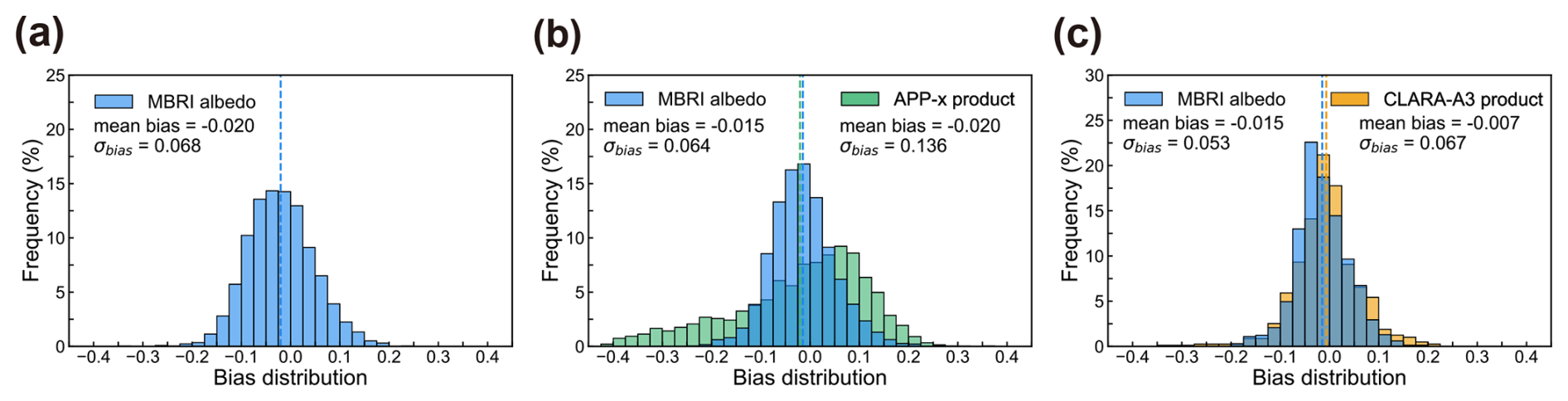
Figure 9 Bias distribution histograms of three albedo products compared to in situ measurements. Blue represents the MBRI albedo product, green represents the APP-x product, and yellow represents the CLARA-A3 product. The dashed line represents the average bias. σ_bias represents the standard deviation of the bias distribution.

Additionally, Fig. 10 presents a representative selection of albedo time series for comparison. Results indicate that after cloudy-sky albedo reconstruction, the MBRI product achieves improved continuity and completeness in the albedo time series across different stations compared to CLARA-A3. The CLARA-A3 product, however, exhibits temporal gaps – notably after day 60 (Fig. 10a and b), before day 275 (Fig. 10c), and at specific points such as day 41 at BSRN SYO (Fig. 10a) and day 287 at Atka AWS2 2012 (Fig. 10d). Owing to its higher temporal resolution, the MBRI product also aligns more closely with rapid changes in the in situ albedo time series. Examples include: (a) BSRN station (Fig. 10a and b): MBRI and in situ time series remain highly synchronized throughout the selected period. Around days 90–96 at SYO, the in situ albedo peaks (∼ 0.93), while the MBRI albedo concurrently rises to approximately 0.96; both decline sharply after day 96. Peak timing and pattern are also consistent at GVN; (b) IMAU AWS17 station (Fig. 10c): Both time series oscillate initially. Between days 300–340, they synchronously rise slightly, then decrease, and rise again after day 340; (c) Atka AWS2 2012 station, the two time series exhibit coordinated fluctuations across the observation period, particularly during periods of significant albedo change (e.g., after day 330).

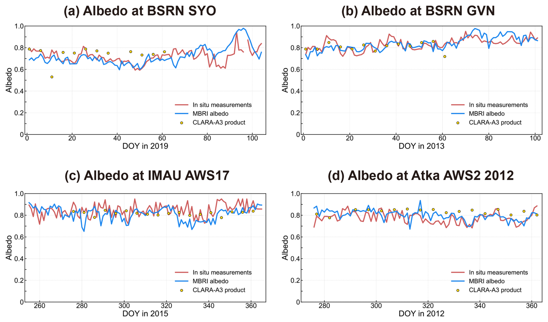
Figure 10 Selected albedo time series at (a) BSRN SYO; (b) BSRN GVN; (c) IMAU AWS17; (d) Atka AWS2 2012. The red line represents in situ measurements, the blue line represents the MBRI albedo product, and the yellow dots represent the CLARA-A3 albedo product.

Overall, the MBRI albedo product proposed in this study demonstrates satisfactory accuracy. The accuracy of the APP-x albedo product is slightly lower, and its RMSE is basically consistent with the validation results of Key et al. (2016). Although the CLARA-A3 product also provides acceptable accuracy, it is less effective than the MBRI product in capturing detailed changes in sea ice, as previously described, due to its relatively coarse temporal resolution and cloud gaps.

4.4 Temporal and spatial difference analysis with the CLARA-A3 product

To assess the applicability of the MBRI albedo product for Antarctic sea ice monitoring, we conducted temporal and spatial comparisons with the CLARA-A3 product. First, the monthly mean albedo anomalies for Antarctic sea ice from 2012 to 2021 were calculated based on the MBRI and CLARA-A3 albedo products. To illustrate the consistency between changes in albedo and sea ice variations, anomalies in the monthly mean SIC and SIE were also calculated, as shown in Fig. 11. The SIC anomaly exhibits a strong correlation with albedo anomalies from both the MBRI (Fig. 11a) and CLARA-A3 (Fig. 11b) products, with correlation coefficients of 0.78 and 0.52, respectively. In terms of temporal variation, before August 2015, most monthly mean anomalies of all three parameters were positive (with only a few exceptions), indicating sea ice accumulation. After this period, SIE anomalies were predominantly negative, while albedo and SIC largely reflected this transition. However, during the summers of 2017–2020, albedo and SIC anomalies were opposite to those of SIE. The driving factors behind this phenomenon warrant further investigation. Additionally, the trends in the monthly mean anomaly sequences from both albedo products are generally consistent, showing an overall decline in sea ice albedo (−0.0002/month for MBRI and −0.0006/month for CLARA-A3). The slight difference in values may be attributed to differences in the algorithms used and the methods for handling cloud gaps. These results indicate that the MBRI albedo product performs well in capturing Antarctic sea ice temporal variability signals.

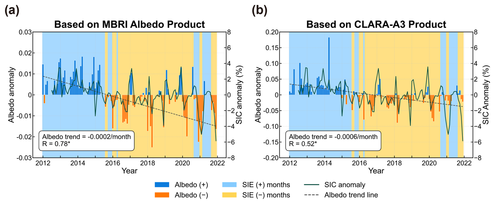
Figure 11 Monthly anomalies of Antarctic sea ice albedo, SIC, and SIE from 2012 to 2021. Albedo anomalies are derived from (a) the MBRI albedo product and (b) the CLARA-A3 product. Blue bars indicate positive (+) albedo anomalies, while orange bars represent negative (−) albedo anomalies. Blue and yellow shaded areas represent months with positive and negative SIE anomalies, respectively. The dark green solid line denotes monthly SIC anomalies, and the black dashed line represents the albedo trend. R represents the correlation coefficient between albedo and SIC. ^* indicates the p-value less than 0.001.

Spatially, three Antarctic sea ice albedo maps in the middle of the month were randomly selected for comparison with the CLARA-A3 product to validate the spatial continuity of the MBRI albedo product (Fig. 12). Although the CLARA-A3 albedo product uses a 5 d average, it still exhibits notable data gap due to the cloud cover. In contrast, the MBRI albedo provides spatially continuous daily albedo data for the sea ice region, with only a few blank strips due to missing raw data. On a broad scale, both products show lower albedo in the marginal ice zone and along the coastline than in stable pack ice areas. To enable a more detailed comparison, the maps of both products were zoomed in on four regions: King Haakon VII Sea (A) in Fig. 12a, the Weddell Sea (B) in Fig. 12b, the Ross Sea (C) and the Prydz Bay (D) in Fig. 12c.

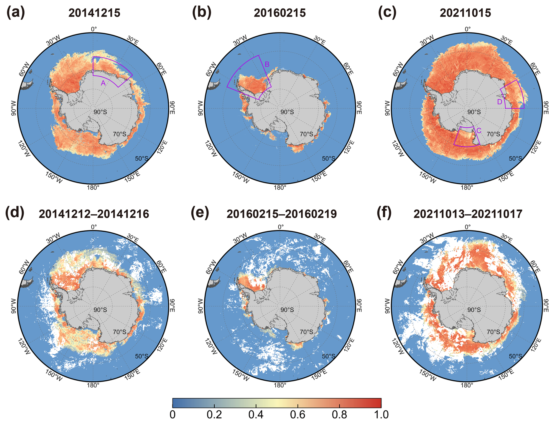
Figure 12 Maps of shortwave albedo for the Antarctic sea ice region. (a)–(c) represent the MBRI albedo on 15 December 2014, 15 February 2016, and 15 October 2021; (d)–(f) show the 5 d averaged CLARA-A3 albedo for the corresponding dates. The purple boxes A–D highlight four areas selected for detailed comparison.

Figure 13 shows a comparison of the MBRI and CLARA-A3 products in selected regions. The albedo spatial distributions of MBRI and CLARA-A3 are highly similar. However, due to its higher spatial resolution, the MBRI albedo captures finer details. For example, in Fig. 13b1 and c1, the sea ice boundaries in the Weddell Sea and along the coastline of the Ross Sea are clearly and accurately defined, with rich texture features such as sea ice leads also being captured. In contrast, the CLARA-A3 product presents these features with relatively less clarity. On the other hand, the coarser resolution of CLARA-A3 may cause pixels to include more open water areas, leading to lower pixel values – especially noticeable at the marginal ice zone (e.g., Fig. 13a2, b2, d2). Therefore, the MBRI albedo product proposed in this study offers a significant spatial resolution advantage, providing more accurate data for research on the Antarctic or regional sea ice.

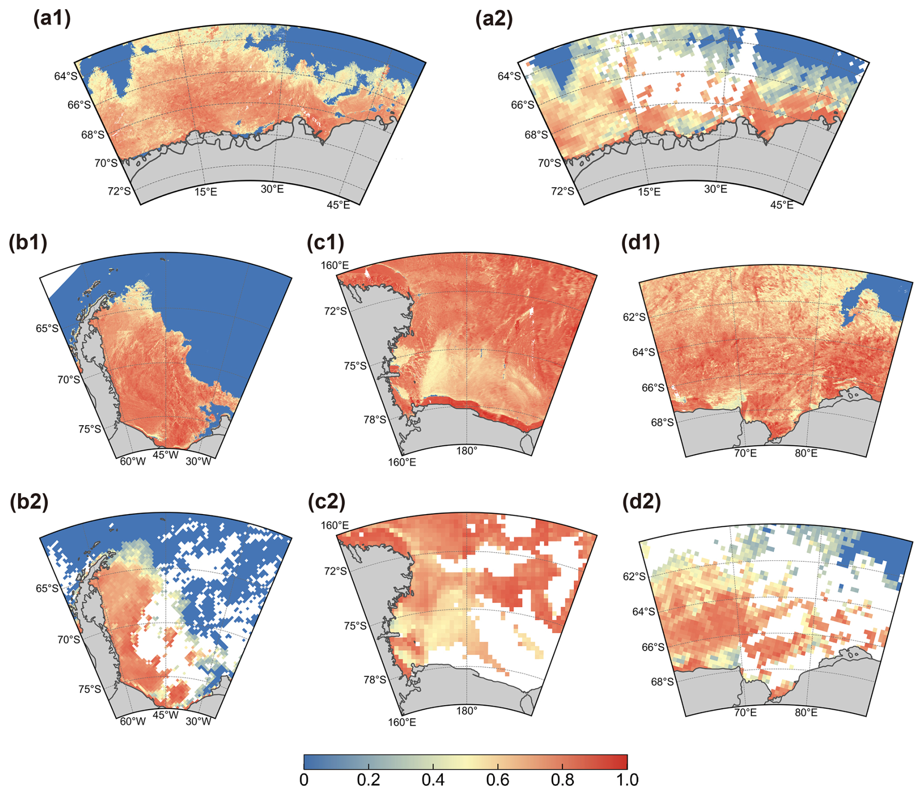
Figure 13 Comparison of shortwave albedo maps in selected regions. (a1)–(d1) show MBRI albedo product maps for the King Haakon VII Sea, Weddell Sea, Ross Sea, and Prydz Bay; (a2)–(d2) show the corresponding CLARA-A3 product maps for these regions.

5 Discussion

The MBRI Antarctic sea ice albedo product offers improvements in spatial and temporal resolution compared to existing datasets, while maintaining high accuracy. This advantage stems primarily the use of a physically-based BRDF model that explicitly accounts for the anisotropy of sea ice surfaces, particularly its strong forward-scattering property. This represents a substantial advancement over models relying on the Lambertian assumption, leading to more accurate sea ice albedo calculations. Validation results (Fig. 7) confirm the MBRI product's superior accuracy compared to existing products. Notably, the CLARA-A3 product correct anisotropy by averaging observations from different angles over multiple days. However, this angular sampling is insufficient, potentially causing underestimation of sea ice albedo (Ding et al., 2022; Qu et al., 2016). The MBRI algorithm leverages multi-band reflectance data from VIIRS, enabling BRDF inversion from single date/angle observations. This avoids the need for temporal compositing, thereby improving temporal resolution. As shown in the time series comparisons (Fig. 10), the daily resolution of the MBRI product effectively captures rapid sea ice changes. Additionally, the 1 km spatial resolution of VIIRS enhances the product's ability to reflect the fine-scale spatial features of sea ice albedo (Fig. 13).

Another advantage is enhanced spatial completeness. We analyzed the MBRI product and in situ measurements under both clear-sky and cloudy-sky conditions to investigate cloud impacts on sea ice albedo. Figure 14 and Table 5 quantify the differences between these conditions. The results show that average albedo under cloudy-sky is significantly higher (by approximately 0.035–0.064, p<0.001) than under clear-sky for both the in situ measurements and the MBRI product, consistent with earlier finding (Key et al., 2001). This indicates that the influence of cloud forcing effects on sea ice albedo cannot be ignored. Furthermore, missing data from either low-albedo marginal ice zones or high-albedo stable pack ice areas can bias regional averages. The stronger correlation between the MBRI albedo anomaly series and SIC anomaly series (Fig. 11) supports this conclusion. Therefore, we consider cloudy-sky albedo reconstruction is necessary for accurately assessing long-term climate change.

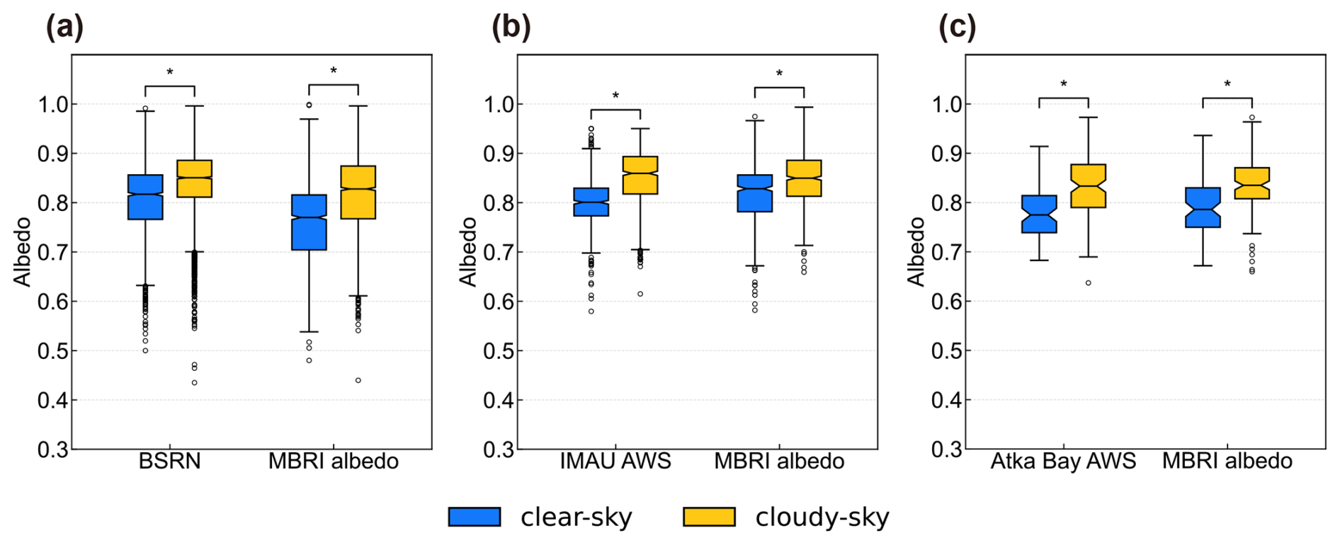
Figure 14 Boxplots of the in situ measurements and MBRI albedo under cloudy-sky and clear-sky conditions. ^* indicates that the difference between clear-sky albedo and cloudy-sky albedo is significant with a p-value less than 0.001.

Table 5 Mean values of in situ measurements and the corresponding MBRI mean albedo at different stations, along with the differences under clear-sky and cloudy-sky conditions.

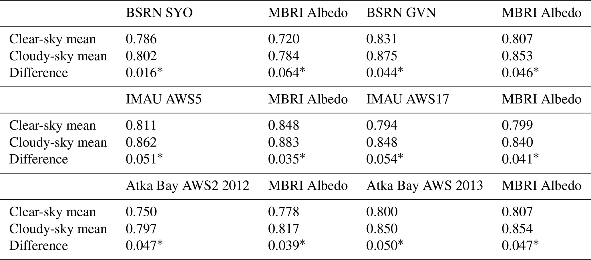
^* indicates that the difference is significant with a p-value less than 0.001.

Despite its advantages, the MBRI product has limitations that can affect spatial and temporal accuracy in specific situations. First, retrieval uncertainty rises significantly (exceeding 0.1) for observations with high VZA in the backward-scatter direction. This issue may arise because the ART model used for the sea ice BRDF, while accurately describing forward-scattering, exhibits higher sensitivity to parameter variations in the backward direction. Although such scenarios are relatively rare, they can introduce inaccuracies in regional albedo analysis. The algorithm's performance at large SZA also requires improvement, as satellite observations under this condition become relatively unreliable. Second, Fig. 3 shows increased uncertainty in low albedo regions like the marginal ice zone and during spring melt. This likely occurs because increased open water and melt ponds in these areas challenge assumptions within the TCOWA model. For instance, sea ice restricts open water movement, altering the relationship between windspeed and wave, and chlorophyll concentrations differ in polar waters compared to open ocean areas. Future work should focus on optimizing these radiative transfer models to enhance their versatility. Finally, cloudy-sky albedo reconstruction relies on spatiotemporal interpolation, introducing higher uncertainty (∼ 0.065). During rapid melt events or extreme weather, these reconstructed values may not fully capture the true, fast-changing albedo. Future research could explore machine learning-based approaches for gap filling to improve reconstruction accuracy.

Given these advantages and limitations, the MBRI product is well suited for studies requiring high spatial resolution and daily temporal scale, including short-term sea ice radiation budget estimation, analysis of regional sea ice albedo changes and feedback assessment, and coupling with regional climate models. For multi-decadal climate trend assessments, the CLARA-A3 albedo product might offer a more consistent long-term baseline. Additionally, during periods of persistent cloud cover, users are advised to use the MBRI product in conjunction with its uncertainty dataset or, where possible, supplement it with ground measurements.

6 Code and data availability

The daily 1 km seamless Antarctic sea ice albedo product (version v2) and the corresponding pixel by pixel uncertainty can be downloaded at https://doi.org/10.5281/zenodo.11216156 (Ma et al., 2024) and https://doi.org/10.5281/zenodo.15067607 (Ma et al., 2025), respectively. These datasets are available from 19 January 2012 to 31 December 2021. These datasets adopt Sinusoidal projection and is gridded using the MODIS Sinusoidal Tile Grid, covering a total of 53 tiles (v14: h06–h29; v15: h09–h26; v16: h11–h17, h21–h24). These datasets are archived in 16-bit integer values GeoTIFF format. The albedo GeoTIFF file contains a single band representing the shortwave blue-sky sea ice albedo, while the uncertainty GeoTIFF file includes a band corresponding to the albedo uncertainty. The data values range from 0 to 10 000, with a scaling factor of 0.0001 applied to convert the integer values to their physical representations. Ocean water and land are set to a filling value of −1.

The sea ice albedo files are named “Antarctic_Sea_Ice_Albedo_yyyyddd_hv.tif”, with “yyyyddd” denoting the date, “hv” representing the number of the tile. For example, “Antarctic_Sea_Ice_Albedo_2014270_h18v15.tif” represents the sea ice albedo data of the h18v15 area on the 270th day of 2014.

The processing codes can be made available upon request to the corresponding author.

7 Conclusions

Sea ice albedo is a key factor influencing the polar radiation budget. Currently, commonly used sea ice albedo products are derived from AVHRR data. These products have relatively low spatiotemporal resolution and large data gaps caused by cloud cover. These disadvantages may limit their application in studies of Antarctic sea ice changes. High spatiotemporal resolution and continuity in Antarctic sea ice albedo products are crucial for investigating the mechanisms behind recent anomalies in Antarctic sea ice. Based on the VIIRS reflectance dataset, we generated a daily 1 km Antarctic sea ice albedo product for the period from 2012 to 2021, with reconstruction of cloudy-sky albedo.

The MBRI algorithm has several advantages compared with traditional methods. First, by considering the heterogeneity and anisotropy of sea ice surface and abandoning the Lambertian assumption, it offers a more accurate reflection of the true surface properties. Second, the MBRI algorithm fully utilizes the sensor's single-angle/date observations, allowing inversion at a 1 km resolution, enhancing the spatial and temporal resolution of the product. Last, when filling cloudy pixels, the algorithm considers the cloud forcing effect on sea ice albedo and corrects it using a physical model, rather than relying on simple spatiotemporal interpolation. These improvements are evident from the comprehensive evaluation carried out in comparison with in situ measurements and existing products.

The validation results with in situ datasets indicate that the MBRI albedo product has an overall RMSE of 0.071, a bias of −0.02, and a correlation coefficient of 0.60. Comparisons at different stations show that MBRI consistently outperforms the APP-x and CLARA-A3 products in terms of accuracy. After spatial and temporal aggregation, the RMSE of MBRI product further decreases (below 0.055). Additionally, time series comparisons at four stations demonstrate that MBRI product provides robust temporal continuity, with daily-scale data basically consistent with in situ measurements. Spatial analysis also reveals that the MBRI product offers spatial continuity and rich spatial details. Therefore, the MBRI albedo product has relatively good overall performance.

Uncertainty analysis indicates that the retrieval process of the MBRI clear-sky albedo remains stable across most geographical locations and observation geometries. The annual average sea ice albedo retrieved uncertainty is 0.022. However, for certain specific observation geometries, such as backward observations at high view zenith angle, the model is more sensitive to parameter variations, which could lead to decreased estimation accuracy (with uncertainties exceeding 0.1). Although such situation is rare, it still requires attention in future research, and improvements in the physical model could potentially enhance the computational robustness under this condition. Additionally, by analyzing albedo values under different sky conditions, it was found that sea ice albedo under cloudy-sky is significantly higher than under clear sky (ranging from 0.035 to 0.064), which highlights the necessity of correcting for cloud radiative forcing effects.

In summary, the MBRI albedo product represents the first daily 1 km seamless Antarctic sea ice albedo dataset. Its demonstrated accuracy and spatiotemporal consistency support its application in quantifying the Antarctic radiative budget, evaluating sea ice albedo feedback, and monitoring sea ice spatiotemporal variations. Future improvements are aimed to refining cloudy-sky albedo reconstruction methods, particularly through improved identification of cloudy pixels and the adoption of advanced remote sensing image reconstruction techniques, to further enhance retrieval reliability under cloudy conditions.