The Dutch real-time gauge-adjusted radar precipitation product

The Dutch real-time gauge-adjusted radar quantitative precipitation estimation (QPE) product provides 5 min accumulations every 5 min on a ∼1 km² grid covering the Netherlands and the area around it ($\sim \mathrm{4.5}\times {\mathrm{10}}^{\mathrm{5}}$ km²). It plays a key role in hydrological decision-support systems and as input for nowcasts in order to inform decision makers. Major changes to the production of this QPE product were implemented on 31 January 2023, and include (polarimetric) fuzzy logic clutter removal, rain-induced attenuation correction, and vertical profile of reflectivity correction. Moreover, the mean-field bias rain gauge adjustment was replaced by a spatially variable rain gauge adjustment. We evaluate the potential quality improvement resulting from these changes by comparing the last year of the old and the first year of the renewed QPE product. Clutter leading to overestimation in the old radar product is effectively removed in the renewed radar product. The evaluation against rain gauge accumulations shows a strong improvement. The average underestimation decreases by about 10 percentage points to 15 % over the Netherlands. Improvements of the statistics are clear for the daily precipitation over a large part of the QPE product domain, but also show the potential for incorporating rain gauge accumulations outside the Netherlands. The 1 h and daily extremes over the Netherlands are also better captured by the renewed product. Improvements in daily precipitation accumulations for the renewed product are stronger in the winter period than in the summer period. Finally, it is recommended to include Belgian and German rain gauge data in the product. The Dutch real-time 5 min gauge-adjusted precipitation radar dataset is publicly available at https://doi.org/10.21944/5c23-p429 (real time) and https://doi.org/10.21944/e7zx-8a17 (archive) (KNMI Radar Team, 2018a, b).

1 Introduction

Accurate, timely, and detailed precipitation information is essential for providing early warnings for extreme precipitation (e.g., for event organization, professionals working outside, and landslide risk), optimizing agriculture, and improving water management (e.g., flash flood forecasting). Rain gauges are accurate but cannot provide the needed coverage, whereas satellite precipitation products have limitations regarding accuracy and spatiotemporal resolution. Ground-based weather radar products do provide the needed space–time coverage. However, many sources of error can limit the usefulness of these products (Doviak and Zrnić, 1993; Fabry, 2015; Rauber and Nesbitt, 2018; Ryzhkov and Zrnic, 2019). To this end, real-time gauge-adjusted radar products optimally combine the accuracy of rain gauges with the coverage of radars.

Peer-reviewed literature providing an overview of the processing of nationwide (near) real-time radar precipitation products and their quality is relatively rare, especially that covering at least all seasons. There are however interesting studies on the quality of real-time quantitative precipitation estimation (QPE) products. Several products cover the conterminous United States of America, such as the NCEP Stage IV radar product (evaluated over an 11-year period by Prat and Nelson, 2015, and Nelson et al., 2016) and the Multi-Radar Multi-Sensor quantitative precipitation system (evaluated over case studies: Zhang et al., 2016; Tang et al., 2020). For Europe, Park et al. (2019) describe a near real-time gauge-adjusted European radar precipitation product and evaluate over May–October for the years 2015–2017. For Switzerland, Germann et al. (2006) present an 8-year evaluation. For the Netherlands, Holleman (2007) provides a 6-year evaluation. For France, Figueras i Ventura and Tabary (2013) describe a single-polarization and two versions of dual-polarization (polarimetric) radar precipitation products, which are evaluated for six radars and a selection of events.

Here, we provide an overview and quality assessment for the Dutch real-time radar QPE product. The Royal Netherlands Meteorological Institute (KNMI) produces a real-time gauge-adjusted radar product of 5 min precipitation accumulations on a ∼1 km² grid every 5 min, which has been publicly available since 19 December 2018 (KNMI Radar Team, 2018a, b). This real-time QPE product covers the Netherlands and the surrounding area ($\sim \mathrm{4.5}\times {\mathrm{10}}^{\mathrm{5}}$ km²; Fig. 1a), and is currently produced with a latency of on average ∼2 min. It is based on data from C-band ground-based weather radars from the Netherlands, Germany, and Belgium, and on data from 32 automatic rain gauges within the Netherlands. Major changes in the production of this QPE product have become operational as of 31 January 2023. These changes include dual-polarization non-meteorological echo removal (Overeem et al., 2020), rain-induced attenuation correction (Overeem et al., 2021), and vertical profile of reflectivity (VPR) correction (Hazenberg et al., 2013). Quality information is derived in each processing step and subsequently used to generate a single surface reflectivity field from volume data for each radar. Further processing includes the statistical Gabella clutter filter (Gabella and Notarpietro, 2002), quality-based compositing of data from the contributing radars, conversion of reflectivity data to 5 min rainfall intensities using the Marshall-Palmer relationship (Marshall et al., 1955), and advection correction. Finally, a spatial adjustment factor field is computed employing 60 min rain gauge accumulations from a previous clock-hour (every hour on the hour). The adjustment factor field is applied to the most recent 5 min precipitation accumulation field.

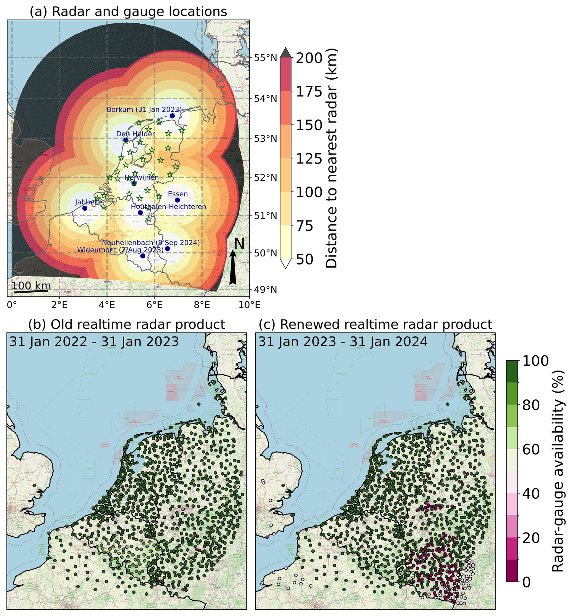
Figure 1 (a) A map with radar (dots) and automatic rain gauge (stars) locations. The background color indicates the distance to the nearest radar, assuming full availability of the radar data (note that some radars, or scans, only contributed part of the period, and the Neuheilenbach radar did not contribute to the datasets studied in this paper) and taking into account their maximum range. (b, c) Maps with combined radar–gauge availability for the daily accumulations from the old (31 January 2022–31 January 2023) and the renewed (31 January 2023–31 January 2024) real-time QPE product. Map data © OpenStreetMap contributors 2025. Distributed under the Open Data Commons Open Database License (ODbL) v1.0.

Machine learning is a promising technique to improve radar-based QPE (e.g., Li et al., 2024) as has for instance been demonstrated with a random forest model trained on 4 years of data and evaluated for six case studies in Switzerland (Wolfensberger et al., 2021). While we do not rule out the future use of machine learning in our operational radar products, we choose to follow a more physically based approach. A disadvantage of machine learning is that it is optimized using a training dataset, and it could hence be vulnerable to changes in radar availability and settings in an unpredictable way. For some processing steps, such as attenuation correction, we expect that this is more robust because it is based on physics and expected to work in a variety of environmental conditions.

The aim of this paper is twofold: first, to describe the datasets and algorithms used to produce this QPE product. Second, to evaluate the quality and limitations for the last year of the old product and for the first year of the renewed product. This is not only relevant for (potential) users of this dataset, but also quantifies the added value of the product renewal. Specific attention is given to the removal of non-meteorological echoes through evaluating maps with annual and maximum precipitation and relative frequency of exceedance. The evaluation is performed utilizing independent hourly and daily rain gauge accumulations by means of annual precipitation accumulation maps, scatter density plots, station-based spatial verification, and metrics as a function of gauge threshold value.

This paper continues with a radar and rain gauge data description (Sect. 2) and an overview of the methodology (Sect. 3). Next, an extensive evaluation of the old and renewed radar products against rain gauge accumulations is presented (Sect. 4), followed by a discussion (Sect. 5). Finally, conclusions and a research and development outlook for this product are provided (Sect. 7).

2 Data

The domain of the Dutch QPE product extends from ∼0–∼10° E and from ∼49–∼56° N, with the Netherlands in the center (Fig. 1a). This region has a temperate, maritime climate. Two datasets are used: a full year before the transition to the new product (31 January 2022–31 January 2023; referred to as the old product) and a full year after this transition (31 January 2023–31 January 2024; referred to as the renewed product).

2.1 Radar data

The real-time radar product evaluated in this study is based on the 5 min volumetric (3D; i.e., a collection of typically 5–15 scans executed at different elevation angles) data from at most seven magnetron-based polarimetric C-band ground-based weather radars. Doppler clutter filtering is applied to both horizontal and vertical reflectivity factor (Z_h and Z_v, respectively) data in order to remove non-meteorological echoes. Two radars are located in the Netherlands, two radars are located in Germany, and three radars are located in Belgium. Fig. 1a shows the locations of these radars including that of an additional radar in Germany (Neuheilenbach) that has been used in the real-time product since 9 September 2024 (i.e., outside the evaluation period). On average 4.8 and 6.1 radars contribute to the real-time product for the old (31 January 2022–31 January 2023) and renewed (31 January 2023–31 January 2024) product, respectively. For both periods, the median number of contributing radars is five. Over a large part of the radar product domain, the distance to the nearest radar is shorter than 150 km (Fig. 1a). Notable are the longer distances to the nearest radar in the Dutch–German border region. More information on the Belgian radars is provided by Goudenhoofdt and Delobbe (2016), on the Dutch radars by Beekhuis and Mathijssen (2018), and on the German radars by Werner (2014).

All radars that are used in this product are calibrated during regular maintenance (1–2 times per year). Monitoring tools are in place at each institute, which can assist to detect drifts in calibration so that action can be taken if this is the case. It is therefore assumed that the calibration of the radars is accurate. For more information on calibration and monitoring, see Beekhuis and Mathijssen (2018) for the Dutch radars, and Frech et al. (2017) for the German radars.

The radar data processing is described in Sect. 3. The end result is a 2D real-time radar product of 5 min accumulations every 5 min on a $\sim \mathrm{1}\mathrm{km}\times \sim \mathrm{1}\mathrm{km}$ grid with almost full data availability. The 5 min accumulations are aggregated to 1 h (every hour on the hour) and daily (ending 00:00, 06:00, or 08:00 UTC) accumulations for comparison against KNMI automatic rain gauge accumulations from the Netherlands (1 h) and against daily rain gauge accumulations from different networks across the entire radar product domain. Accumulations were only computed when data availability was at least 83.3 %. The annual accumulations were generated without this data availability criterion.

The combined daily radar–gauge availability is generally 95 % or higher (Fig. 1b and c). Lower availability is caused by missing gauge records. The exception is that for the renewed radar product the lower availability for the (south)western and southeastern part of the product domain is caused by lower radar data availability. This extended coverage with lower availability can be attributed to the Wideumont radar in the southeast that started contributing in August 2023 and the addition of longer range scan data from the Jabbeke radar in the southwest.

2.2 Rain gauge data

2.2.1 KNMI 10 min and hourly automatic rain gauge data

KNMI operates an automatic rain gauge network that electronically measures precipitation accumulations based on the displacement of a float placed in a reservoir (KNMI, 2000). The locations of these 32 gauges, with a density of ∼1 gauge per 1000 km² over the land surface of the Netherlands, are displayed in Fig. 1a. The unvalidated 10 min data were aggregated to 1 h precipitation accumulations (every hour on the hour). Only these accumulations were used to compute a spatial adjustment factor field for real-time radar product adjustment. In addition, validated 1 h gauge accumulations (every hour on the hour) were obtained for evaluation purposes. Since the automatic gauge accumulations from a previous clock-hour (every hour on the hour) are employed in the adjustment, the evaluation is considered to be independent.

2.2.2 KNMI daily manual rain gauge data

The manual rain gauge network operated by KNMI provides daily precipitation accumulations (the end time of observation is 08:00 UTC) from 317 (old product) and 319 (renewed product) gauges (density of ∼1 gauge per 100 km²). Volunteers empty these rain gauges at 08:00 UTC and pass on the readings to KNMI (KNMI, 2000). Here, the accumulations that have been validated by KNMI staff are employed for evaluation purposes. For qualitative comparison purposes, a product with spatially interpolated daily rain gauge accumulations at a 1 km×1 km grid over the Netherlands is used (Soenario et al., 2010; Siegmund, 2014).

2.2.3 DWD daily rain gauge data

Daily manual and automatic rain gauge accumulations over Germany were obtained on 6 December 2024 from the German Weather Service (DWD) open data portal Climate Data Center (DWD, 2024); the “historical”, more quality-controlled data were available through 31 December 2023, and as of 1 January 2024 the “recent” less quality-controlled data were employed. These accumulations are utilized for the spatial evaluation for 468 locations (old radar product) and 649 locations (renewed radar product). The end time of observation is 06:00 UTC.

2.2.4 ECA&D daily rain gauge data from Belgium, France, Luxembourg, and the United Kingdom and the E-OBS dataset

The non-blended daily precipitation accumulations were obtained on 20 December 2024 from the European Climate Assessment and Dataset (ECA&D, https://www.ecad.eu, last access: 23 January 2025) project (Klein Tank et al., 2002; Klok and Klein Tank, 2008) and are used for the spatial evaluation. This concerns rain gauge data from 170–171 locations in Belgium (end time of observation 00:00 UTC) and Luxembourg (end time of observation 00:00 UTC), 50–64 locations in France (end time of observation 08:00 UTC), and 2–8 locations in the United Kingdom (end time of observation 08:00 UTC). This includes non-downloadable series (i.e., included in ECA&D for the production of derived data but only accessible through the data owner). These data have been quality controlled by the ECA&D team (Project team ECA&D, Royal Netherlands Meteorological Institute KNMI, 2021) and often also by the party that has delivered the data. Instead of the ECA&D, the German rain gauge data were retrieved from their original source, the DWD open data portal.

For qualitative comparison purposes, a spatially interpolated daily ECA&D rain gauge accumulation product over Europe is used (E-OBS version 30.0e; Cornes et al., 2018; Copernicus Climate Change Service, 2024). This dataset was aggregated to annual precipitation accumulations.

3 QPE production

Production of the QPE product involves several processing steps, starting with steps that are applied for each radar separately. This is followed by processing steps that are done on the combined product. These two collections of steps are shown as flowcharts in Fig. 2, ultimately leading to the renewed real-time radar product. The production process for the old radar product lacks most of these processing steps and is summarized in the next subsection.

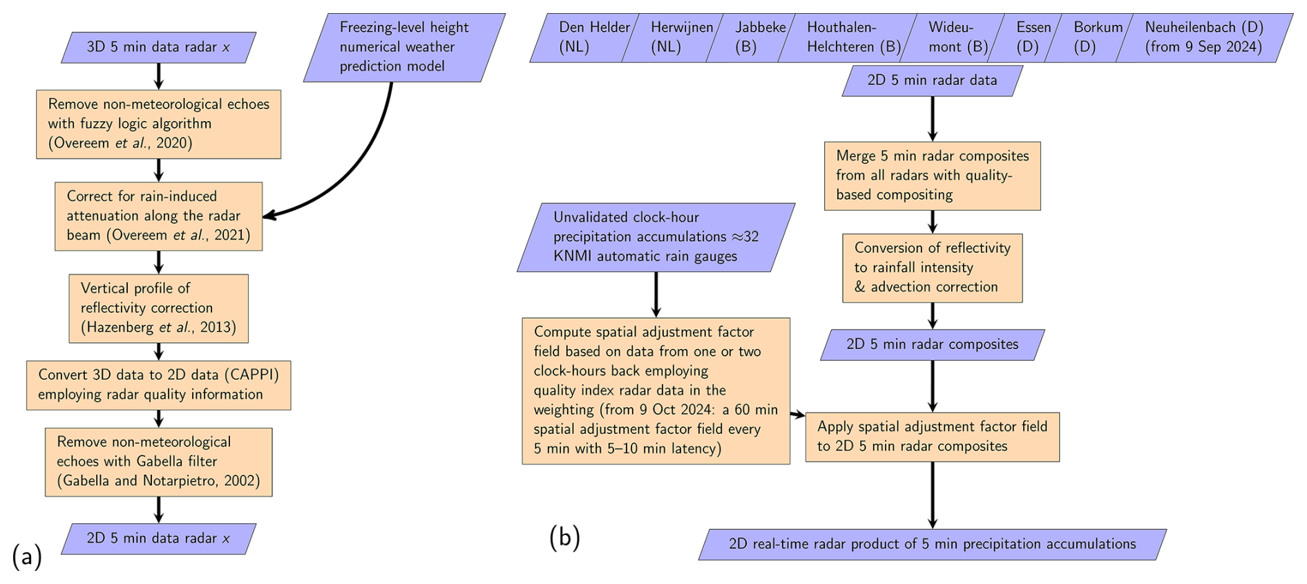
Figure 2 Flowcharts of the real-time QPE production chain: (a) for single radar processing; (b) for the combined radar and rain gauge data.

3.1 Processing the old radar product

For each radar, a 2D radar pseudo-constant-altitude plan position indicator (pseudoCAPPI) of Z_h is produced by logarithmic averaging of the Z_h (dBZ_h) data from three scans. This is converted to precipitation intensities R through a Z_h=200R^1.6 relationship (Marshall et al., 1955). A constant mean-field bias adjustment factor is subsequently applied to this intensity field (Holleman, 2007). The mean-field bias adjustment factor is based on radar and rain gauge 1 h accumulations from a previous clock-hour (every hour on the hour; as explained in Sect. 3.9). The resulting intensity fields from each radar are transformed to 5 min accumulations and subsequently combined into a single 2D composite via range-weighted compositing.

3.2 Fuzzy logic clutter removal

The processing for the renewed radar product starts with the removal of non-meteorological echoes (clutter) by employing the fuzzy logic algorithm from the wradlib open-source Python library for weather radar data processing (Heistermann et al., 2013; Overeem et al., 2020; Mühlbauer et al., 2020). The clutter results from reflections of non-meteorological targets, such as the ground, buildings, trees, cars, sea surface, ships, birds, and planes. This may be exacerbated by anomalous propagation leading to the beam hitting the ground or sea surface. Interference by other sources of radio waves such as wireless networks and the sun also cause clutter (Gourley et al., 2007; Fabry, 2015; Huuskonen et al., 2016; Saltikoff et al., 2016). Removal of clutter-affected data is important, since they can lead to severe precipitation overestimation.

The fuzzy logic algorithm uses decision variables to classify clutter for each voxel from each scan separately (Vulpiani et al., 2012; Crisologo et al., 2014; Overeem et al., 2020). The following decision variables are employed for the Dutch radar data, with their weight provided between brackets: texture (spatial variability) of the differential reflectivity (Z_DR; 0.20), the copolar correlation coefficient (ρ_HV; 0.15), texture of ρ_HV (0.25), depolarization ratio (0.20) (Ryzhkov et al., 2017), and clutter phase alignment (0.20) (Hubbert et al., 2009a, b). For each decision variable, the degree of membership to the meteorological target class is calculated employing a membership function. A weighted average of the degree of membership to the meteorological target class is computed using all decision variables, each having its own weight. A voxel is classified as clutter if this weighted average is below a threshold value of 0.6. In that case the associated Z_h is set to the “nodata” value (i.e., areas void of data). All details regarding the fuzzy logic algorithm and its (parameter) settings are provided by Overeem et al. (2020).

The Belgian radar data lack the decision variable clutter phase alignment. Utilizing the same membership functions, only three decision variables are used and with a different weight: texture of Z_DR (0.5), texture of the two-way differential propagation phase (0.3), and ρ_HV (0.2). Moreover, the employed threshold value in the classification is 0.3.

Goudenhoofdt and Delobbe (2016) give more information on the Belgian radar processing. For the German radars, no polarimetric data were publicly available for the periods that are used in this paper. However, DWD has already applied several post-processing algorithms, including a (partly polarimetric) fuzzy logic clutter detection and removal algorithm for the two 1-year periods. Werner (2014) provide details on the German radar processing.

3.3 Attenuation correction

Rain-induced attenuation can lead to severe precipitation underestimation for C-band weather radars (Hitschfeld and Bordan, 1954; Tabary et al., 2009; Fabry, 2015). The two-way path-integrated attenuation (PIA) along the radar beam can be estimated and corrected for. Here, the recipe from Overeem et al. (2021) is followed. Horizontal specific attenuation is computed from the specific differential phase (K_dp) (Bringi et al., 1990) assuming a linear relation between the two for the Belgian and Dutch radars (k_h=0.081K_dp). Because real-time access to dual-polarization data from the German radars was not possible, a Hitschfeld–Bordan type of algorithm was applied there. This method, called the modified Kraemer method, uses the method proposed by Hitschfeld and Bordan (1954) with an additional limit on the attenuation correction of 10 dB and on the resulting reflectivity of 59 dBZ_h to avoid instability of the algorithm (Jacobi and Heistermann, 2016; Overeem et al., 2021). The final step for both methods is to increase the Z_h value for each voxel by the computed attenuation. The method using K_dp was shown to outperform the modified Kraemer method using 1 year of data from the two C-band radars in the Netherlands, but the stability of the modified Kraemer method was also confirmed (Overeem et al., 2021).

For both methods, the wradlib open-source Python library for weather radar data processing (Heistermann et al., 2013; Mühlbauer et al., 2020) is utilized. Since the correction is meant for attenuation caused by liquid precipitation, a voxel is only used to compute the attenuation in case its height is below the forecasted freezing-level height from the numerical weather prediction model HARMONIE-AROME. And for the method using K_dp, voxels classified as clutter are not employed to compute attenuation (Wradlib, 2020b). Attenuation correction is applied to all voxels, so also those above freezing-level height.

For the German radars, for which no polarimetric data were available, the modified Kraemer method is applied per elevation scan via the $k_{\mathrm{h}}=\mathit{\alpha }{Z}_{\mathrm{h}}^{\mathit{\beta }}$ relation. The values of α and β are reduced from their initial values in an iterative procedure until the constraints Z_h,cor≤59 dBZ_h and PIA≤10 dB are met. In case constraints are not met, no attenuation correction is performed. More details are provided by Jacobi and Heistermann (2016), Overeem et al. (2021), and Wradlib (2020a).

Here, the algorithm of Overeem et al. (2021) is extended to attenuation correction for vertically polarized reflectivity, employing k_v=0.058978K_dp, in order to obtain the attenuation-corrected Z_DR. This is important, since it is used in the VPR correction.

3.4 Vertical profile of reflectivity correction

Precipitation generally has a non-uniform vertical structure. Therefore, the increased height of the radar sampling volume at a long range can lead to errors in surface precipitation estimates. To address this, the VPR correction is applied as suggested by Hazenberg et al. (2013, 2014), extended with the polarimetric melting layer detection from Boodoo et al. (2010). The algorithm estimates two idealized VPR profiles, one for stratiform, and one for undefined precipitation based on all data that have been classified as one of these two precipitation types. Note that no VPR estimation or correction is applied for convective precipitation because there is much more vertical mixing in convection. The VPR estimates include an uncertainty estimate that is used in subsequent steps of the QPE processing chain. The VPR estimates are then used to extrapolate all reflectivity data down to the ground. For both estimation and correction for the VPR, the shape of the beam is assumed to be Gaussian.

3.5 Quality-based merging of radar scans

We use quality information to combine data from several scans to derive a 2D surface reflectivity product. Appendix A details the estimation of a quality index Q_T for each voxel. The N voxels that contribute to a given pixel in the 2D surface reflectivity product are combined as follows into a quality-weighted reflectivity (Z_h,Q):

$$\begin{array}{}\text{(1)}& Z_{\text{h,Q}}={\displaystyle \frac{{\sum }_{j=\mathrm{1}}^N{Q}_{\mathrm{T},j}{Z}_{\mathrm{h},j}}{{\sum }_{j=\mathrm{1}}^N{Q}_{\mathrm{T},j}}},\end{array}$$

where both reflectivities are expressed in mm⁶ m⁻³.

A combined quality index is also computed for each pixel in the 2D radar product (Q_r). The basic principles are that each added voxel j raises the value of the quality index, and that the resulting quality index ranges between 0 and 1:

$$\begin{array}{}\text{(2)}& Q_{\mathrm{r}}=\mathrm{1}-\prod _{j=\mathrm{1}}^N(\mathrm{1}-Q_{\mathrm{T},j}).\end{array}$$

The advantage of this approach is that voxels from scans that have a non-zero quality can compensate for the zero quality of voxels from other scans, and that voxels with a lower quality have a much lower weight in the final product.

3.6 Gabella clutter filter

The Gabella clutter filter from the wradlib open-source Python library for weather radar data processing (Gabella and Notarpietro, 2002; Heistermann et al., 2013; Mühlbauer et al., 2020; Wradlib, 2020c) has been successfully applied for the detection and removal of residual clutter (e.g., RADKLIM for Germany and EURADCLIM for Europe; Lengfeld et al., 2019; Overeem et al., 2023a). Here, it is applied to the 2D Cartesian Z_h,Q data from each radar and time interval separately. First, large gradients of Z_h,Q in space are detected. For each central pixel, the number of pixels within a square lattice of 5×5 pixels is counted that have a Z_h,Q value less than 6 dB lower than the central pixel. The central pixel is classified as clutter if this number of pixels is fewer than six. Second, the ratio between the area and circumference for contiguous echo areas with Z_h,Q above 0 dBZ_h is calculated. The central pixel is classified as clutter if this ratio is lower than 1.3 pixels. The central pixels classified as clutter do not contribute to the radar product by setting the Z_h to the “nodata” value and the quality index to 0.

3.7 Compositing of reflectivity images

The radar quality index (Appendix A) is also used to weigh the reflectivity values from individual radars into a combined composite of Z_h,Q. It employs the same algorithms as for the construction of 2D surface reflectivity products for each radar: the quality weighted Z_h is computed using Eq. (1) and the corresponding quality index is computed using Eq. (2).

3.8 Conversion to rainfall intensities and advection correction

Reflectivities Z_h,Q (mm⁶ m⁻³) are converted to rainfall intensities R (mm h⁻¹) employing the Z_h,Q –R relationship (Marshall et al., 1955):

$$\begin{array}{}\text{(3)}& Z_{\text{h,Q}}=\mathrm{200}{R}^{\mathrm{1.6}}.\end{array}$$

This implicitly assumes that the precipitation is liquid, i.e., rain.

Storms that move more than 1 km (the spatial resolution of the QPE product) in 5 min (its temporal resolution) will lead to artifacts in precipitation accumulations. This is corrected by interpolating radar composites in time. For this purpose, advection vectors are computed using the implementation of Farnebäck (2003) in the OpenCV library (http://opencv.org, last access: 4 February 2025). These vectors are then used to interpolate the radar composites in time. The resulting interpolated precipitation intensity becomes a weighted average of the previous (t=t₀) and current (t=t₁) precipitation composite:

$$\begin{array}{}\text{(4)}& \begin{array}{r}{R}_{\text{int}}(\mathit{x},t)={\displaystyle \frac{t_{\mathrm{1}}-t}{t_{\mathrm{1}}-t_{\mathrm{0}}}}R(\mathit{x}+\mathit{v}(t-t_{\mathrm{0}}),t_{\mathrm{0}})+\\ {\displaystyle \frac{t-t_{\mathrm{0}}}{t_{\mathrm{1}}-t_{\mathrm{0}}}}R(\mathit{x}-\mathit{v}(t_{\mathrm{1}}-t),t_{\mathrm{1}}),\end{array}\end{array}$$

with t the time ($t_{\mathrm{0}}\le t\le t_{\mathrm{1}}$), R_int(x,t) the interpolated precipitation intensity, R(x,t) the composite precipitation intensity, x the location of the pixel, and v the advection vector (m s⁻¹). Subsequently, the advection-corrected 5 min precipitation accumulation is computed by aggregating a number of interpolated composites and multiplying by the time interval between the different interpolated composites:

$$\begin{array}{}\text{(5)}& R_{\text{acc}}(x,t_{\mathrm{1}})={\displaystyle \frac{t_{\mathrm{1}}-t_{\mathrm{0}}}{N+\mathrm{1}}}\sum _{i=\mathrm{0}}^N{R}_{\text{int}}\left(x,t_{\mathrm{0}}+i{\displaystyle \frac{t_{\mathrm{1}}-t_{\mathrm{0}}}{N}}\right),\end{array}$$

where N−1 is the number of composites that is generated between the previous (t₀) and present (t₁) composite. Since the horizontal velocity of showers is expected to be lower than 50 m s⁻¹, N=14 is used for this spatiotemporal resolution (1 km and 5 min).

3.9 Gauge adjustment of radar accumulations

The method for the adjustment of radar accumulations with rain gauge accumulations is a modified version of Barnes' objective analysis (Barnes, 1964). The aim is to have a method that is robust in situations with large precipitation gradients and limited gauge density, and that can use quality information of both the radar and rain gauge precipitation estimates. The spatial adjustment factor for a given pixel is computed by the ratio of distance-weighted sums of the unadjusted radar and corresponding rain gauge precipitation accumulations at the gauge locations. The computation of the spatial adjustment factor field is described in Appendix B. Although the adjustment factor field itself is computed based on radar and gauge accumulations from the same 60 min interval, it does not encompass the radar data from the current 5 min time interval due to the 50 min latency of gauge data, that were only available every clock-hour (every hour on the hour). Hence, the adjustment factor field from a previous clock-hour (every hour on the hour) was used. For instance, from 10:50–11:50 UTC the 5 min accumulations were adjusted employing the spatial adjustment factor field based on 60 min radar and gauge accumulations from 09:00–10:00 UTC. As of 11:50 UTC, the applied spatial adjustment factor field was computed based on data from 10:00–11:00 UTC. And possibly, sometimes even an older adjustment factor field was employed.

4 Evaluation results

The performance of the old radar product in its last year is compared to the performance of the renewed radar product in its first year. The performance evaluation is done by qualitative analysis of maps of accumulations and exceedance probabilities as well as by quantitative comparison against rain gauge accumulations. Statistics are presented as a function of gauge accumulation threshold value, geographic location, and season.

Radar precipitation accumulations from pixels directly above a rain gauge (R_radars) are evaluated against the corresponding rain gauge precipitation accumulations (R_gauges). Residuals are defined as the radar accumulations minus the corresponding gauge accumulations. The following metrics are computed:

• The relative bias is the mean of the residuals divided by the mean of the gauge accumulations. It is expressed as a percentage:

  $$\begin{array}{}\text{(6)}& \begin{array}{rl}\text{Relative bias}& ={\displaystyle \frac{{\stackrel{\mathrm{‾}}{R}}_{\text{res}}}{{\stackrel{\mathrm{‾}}{R}}_{\text{gauges}}}}\times \mathrm{100}\\ & ={\displaystyle \frac{{\sum }_{i=\mathrm{1}}^n{R}_{\text{res},i}}{{\sum }_{i=\mathrm{1}}^n{R}_{\text{gauges},i}}}\times \mathrm{100},\end{array}\end{array}$$

  with n the total number of radar–gauge pairs.

• The coefficient of variation of the residuals (CV_res, called CV in this paper) is computed as the standard deviation of the residuals, divided by the mean of the gauge accumulations:

  $$\begin{array}{}\text{(7)}& {\text{CV}}_{\text{res}}={\displaystyle \frac{\sqrt{\frac{\mathrm{1}}{n-\mathrm{1}}{\sum }_{i=\mathrm{1}}^n(R_{\text{res},i}-{\stackrel{\mathrm{‾}}{R}}_{\text{res}}{)}^{\mathrm{2}}}}{{\stackrel{\mathrm{‾}}{R}}_{\text{gauges}}}}.\end{array}$$

  This is a measure of the spread.

• The Pearson correlation coefficient (ρ) or its squared value (ρ²) between the radar and gauge accumulations is computed:

  $$\begin{array}{}\text{(8)}& \mathit{\rho }={\displaystyle \frac{\text{cov}(R_{\text{gauges}},R_{\text{radars}})}{s\left(R_{\text{gauges}}\right)\times s\left(R_{\text{radars}}\right)}},\end{array}$$

  with s the sample standard deviation.

• The Kling–Gupta efficiency (KGE) is computed to summarize performance in one score (Kling et al., 2012):

$$\begin{array}{}\text{(9)}& \text{KGE}=\mathrm{1}-\sqrt{(\mathit{\rho }-\mathrm{1}{)}^{\mathrm{2}}+(\mathit{\beta }-\mathrm{1}{)}^{\mathrm{2}}+(\mathit{\gamma }-\mathrm{1}{)}^{\mathrm{2}}},\end{array}$$

with the bias ratio β (being equal to the relative bias + 1):

$$\begin{array}{}\text{(10)}& \mathit{\beta }={\displaystyle \frac{{\stackrel{\mathrm{‾}}{R}}_{\text{radars}}}{{\stackrel{\mathrm{‾}}{R}}_{\text{gauges}}}}.\end{array}$$

The variability ratio γ is given by

$$\begin{array}{}\text{(11)}& \mathit{\gamma }={\displaystyle \frac{{\text{CV}}_{\text{radar}}}{{\text{CV}}_{\text{gauge}}}}={\displaystyle \frac{s_{\text{radar}}/{\stackrel{\mathrm{‾}}{R}}_{\text{radar}}}{s_{\text{gauge}}/{\stackrel{\mathrm{‾}}{R}}_{\text{gauge}}}}.\end{array}$$

The chosen metrics are often employed for verification purposes. The CV is the standard deviation of the residuals divided by the mean of the reference, here the rain gauges. Values for the root mean square error (RMSE) will generally increase for regions with on average higher rainfall amounts. The reason to use the CV instead of RMSE is that it facilitates comparisons between studies, because it takes the average climatic conditions into account by normalizing with the mean rainfall of the reference. Furthermore, the CV is a better measure of the scatter than the RMSE because it is not affected by the bias. Mean absolute error (MAE) is a similar metric, but puts less emphasis on outliers than the RMSE and CV, but is also affected by the bias. The Pearson correlation coefficient describes the degree of covariation between the estimate and the reference, hence adding more insight into the performance.

The relative frequencies of exceedance are computed for each pixel separately and obtained by dividing the number of exceedances by the number of values with data (i.e., not equal to the “nodata” value, denoting outside the radar product domain). Missing radar files are not taken into account in the computation of the number of exceedances and the number of values with data.

4.1 Qualitative analyses

Maps of the maximum 5 min precipitation accumulation over 1 year as shown in Fig. 3a and b reveal values of 10 mm and higher. These are mostly associated with shipping tracks and wind farms over the North Sea and the English Channel, and metal cranes and containers of the Port of Rotterdam (“Maasvlakte (2)”) for the old radar product (Fig. 3a). They are hardly present in the renewed radar product, showing the effectiveness of the fuzzy logic algorithm and the Gabella clutter filter, with only some remaining isolated spots that are probably due to wind farms (Fig. 3b). Clutter for the land surface is less of an issue than sea clutter, which is clearly visible for the old radar product. Maps of the relative frequency of 5 min precipitation ≥0.01 and >6 mm h⁻¹ for the old radar product (Fig. 3c and e) reveal clutter for “Maasvlakte (2)”, shipping tracks (much more pronounced for 6 mm h⁻¹) and wind farms in the North Sea, and quite some suspicious areas for the land surface that are likely clutter. Few clutter areas appear in the renewed radar product, except for the radial patterns over the North Sea and the English Channel for ≥0.01 mm h⁻¹, pointing toward the Belgian radar in Jabbeke, which are caused by interference (Fig. 3d).

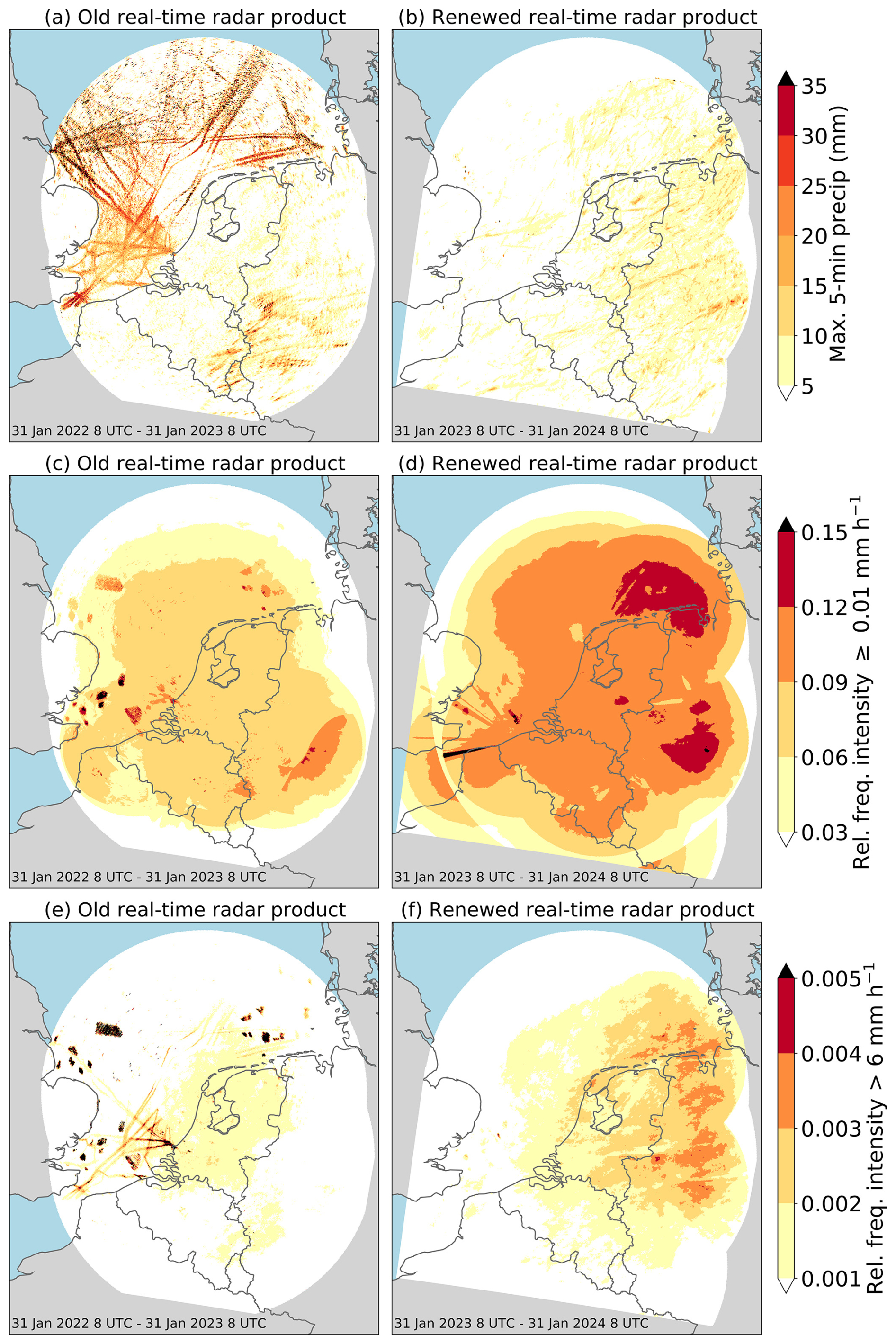
Figure 3 (a, b) Maps of maximum 5 min precipitation accumulation and (c–f) maps of the relative frequency of 5 min precipitation ≥0.01 and >6 mm h⁻¹. For the old (left panels a, c, e) and renewed (right panels b, d, f) radar product. No data availability criterion has been applied. Made with Natural Earth.

Fig. 3 shows that to some extent the maximum accumulations, but especially the relative frequencies of exceeding a threshold, are generally larger for the renewed radar product. This could be partly due to the much wetter 1-year period, but also indicates lower underestimation due to improved processing. Note the high 5 min maxima in the southeastern part for the old radar product, which seem connected to rain showers. The spatial patterns here are typical for storms that move faster than a single pixel (1 km) in the time between two samples (5 min). The renewed product (Fig. 3b) does not exhibit such patterns, indicating that the advection correction (see Sect. 3.8) is effective.

The annual precipitation maps (Fig. 4a and c) reveal all the types of artifacts found in Fig. 3, confirming that clutter is a large issue for the old radar product, whereas it is mainly limited to a single spoke-like artifact caused by interference for the renewed radar product, resulting in accumulations of 1420 mm or higher.

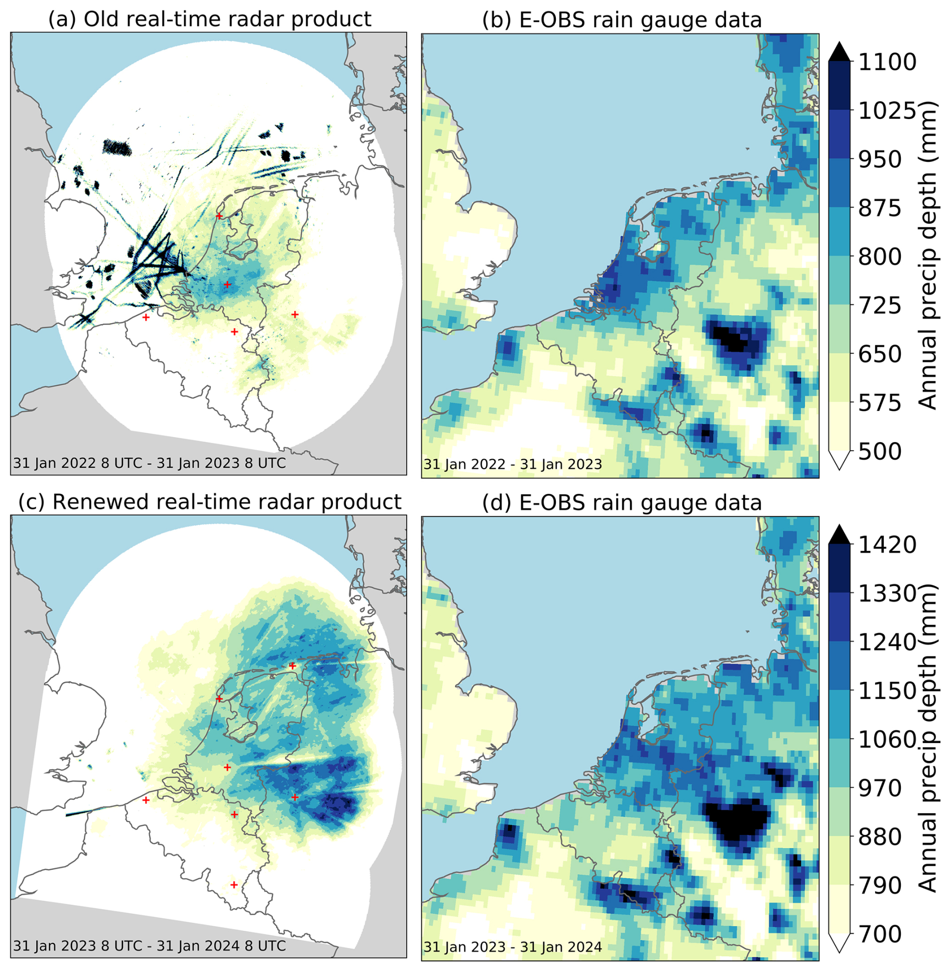
Figure 4 Annual precipitation accumulations for (a) the old radar product (∼1 km²) and for (b) interpolated rain gauge observations (E-OBS version 30.0e; release September 2024; 0.1°×0.1°). (c, d) The accumulations for the renewed radar product and E-OBS. The red crosses in (a, c) denote the radar locations. Made with Natural Earth.

4.2 Annual precipitation maps

Fig. 4 shows the annual precipitation maps for the old and renewed radar products and the corresponding E-OBS interpolated rain gauge product. The old radar product severely underestimates the precipitation, especially outside the Netherlands, where no gauge accumulations have been employed in the adjustment. Underestimation is less severe for the renewed radar product. Precipitation gradients over the Netherlands roughly coincide with the E-OBS gauge product. The large area with high precipitation accumulations in Germany, that is missed in the old radar product, is captured by the renewed radar product. This is likely the result of the much higher weight of data from the nearest radar in the compositing and, to a lesser extent, the added value of the VPR correction, the rain-induced attenuation correction, and the contribution of the Borkum radar.

The effect of severe beam blockage can be noticed in the east and northeast of the Netherlands for both products, pointing towards the Dutch Herwijnen radar (see Fig. 1). For the old product, beam blockage becomes apparent only at longer range from the radar, where the precipitation estimation is mainly based on the data from the Herwijnen radar (other radars have much more weight close to the radar). The severe beam blockage in the easterly direction from the Herwijnen radar, mainly caused by a line of trees, underpins the need for radar site protection. The effects of beam blockage over the northeast of the Netherlands, mainly caused by orography by the Utrecht Hill Ridge (Overeem et al., 2023b), is decreased for the renewed radar product due to the mitigating effect of the addition of data from the German radar in Borkum (Fig. 1a).

4.3 Scatter density plots

Scatter density plots and metrics of radar versus rain gauge precipitation accumulations are employed to assess the overall performance of the radar product for the Netherlands. For both 1 h and daily precipitation accumulations, the renewed radar product performs better than the old radar product (Fig. 5). Notably, the underestimation decreases from ∼17 % to ∼7 % for hourly and from ∼24 % to ∼15 % for daily accumulations. But also the values for CV are lower and the values for ρ² and KGE are higher for the renewed radar product. The improvements for the renewed radar product are more apparent in the daily scatter density plots than in the hourly plots through better alignment along the 1:1 line. The fact that underestimation by the radar is lower in magnitude compared to the automatic rain gauges than in comparison to the manual rain gauges is consistent with the finding reported in Brandsma (2014), namely that automatic rain gauges are biased low by 5 %–8 % compared to manual rain gauges. Since clutter leads to overestimation and is more severe for the old radar product, it partly compensates for the mean underestimation. This implies that the underestimation for true precipitation events in the older radar product is actually larger than indicated in Fig. 5. This is confirmed by the many outliers for (near) zero daily gauge accumulations (and a few outliers for 1 h accumulations) that are not visible anymore in the renewed radar product. Hence, the improvement in the bias may be even larger.

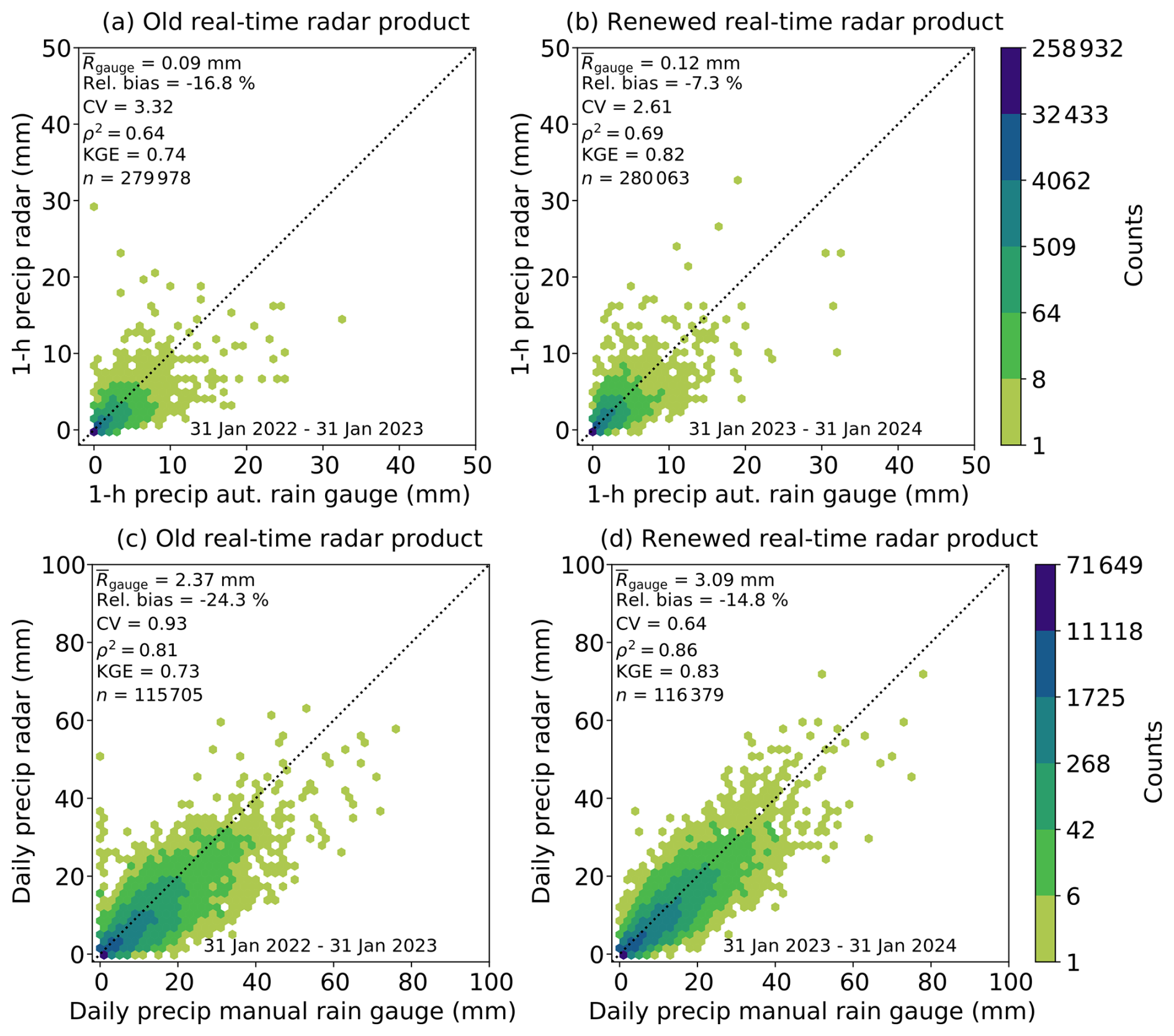
Figure 5 Scatter density plots of (a, b) 1 h and (c, d) daily radar precipitation accumulations against, respectively, independent automatic and manual KNMI rain gauge accumulations from the Netherlands for the old (left panels a, c) and renewed (right panels b, d) radar product.

4.4 Summer storm Poly

An example of the capability of the renewed radar product for real-time precipitation monitoring is shown in Fig. 6. Summer storm Poly struck the Netherlands on 5 July 2023 with locally more than 25 mm in 24 h (Fig. 6a and b). Daily precipitation patterns and accumulations from the radar product match quite well with those from an interpolated rain gauge product, based on validated data from 319 rain gauges from the Netherlands. Only the radar product is available in real time and provides much more spatial detail and can hence capture the counterclockwise rotational movement of the low pressure area (Movie S1 in the Supplement). The scatter density plot shows a fairly high correspondence of the daily radar accumulations with the manual rain gauge accumulations from the Netherlands. It is expected that the old product performs less well primarily because of the lack of attenuation correction.

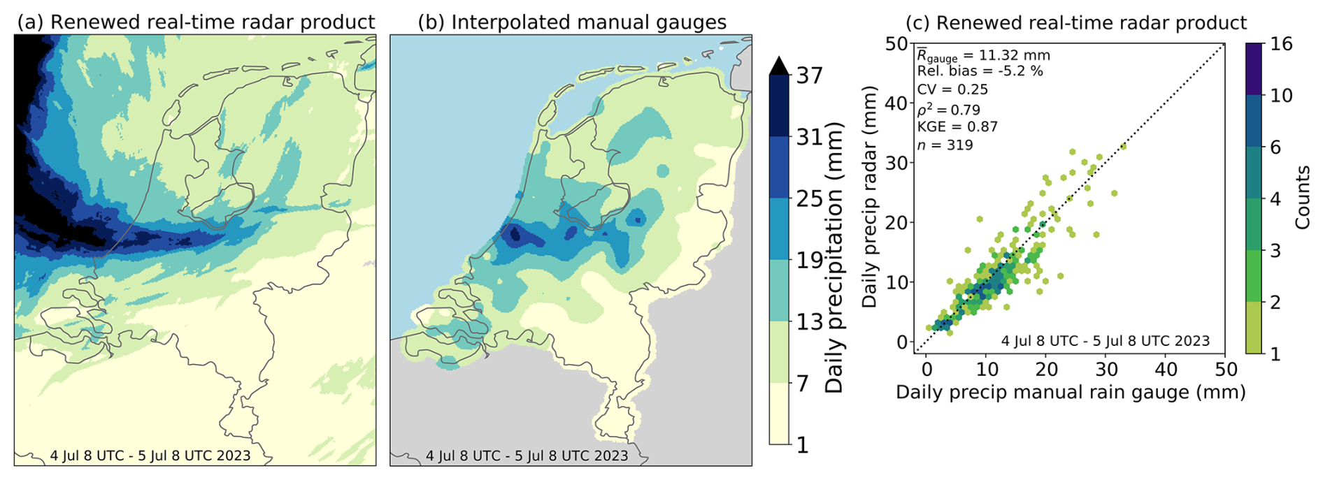
Figure 6 Daily precipitation accumulations caused by summer storm Poly for (a) the renewed radar product and for (b) independent interpolated daily manual rain gauge observations for the Netherlands. (c) A scatter density plot of daily radar precipitation accumulations for the renewed radar product against independent rain gauge accumulations from KNMI's manual network from the Netherlands. The 5 min precipitation accumulations from 5 July 2023 03:55–08:00 UTC are presented as the Supplement (Movie S1). Made with Natural Earth.

4.5 Spatial evaluation

The performance of daily radar precipitation accumulations is quantified for 1008 (old radar product) and 1210 (renewed radar product) rain gauge locations employing independent daily gauge accumulations from networks in Belgium, France, Germany, Luxembourg, the Netherlands, and the United Kingdom at their default measurement interval (Fig. 7; note that this does not include the KNMI automatic gauges used for adjustment). Underestimation is severe for the old radar product (Fig. 7a), especially when the distance to the nearest employed automatic gauge from the Netherlands and to the nearest radar is long (Fig. 1a). The renewed radar product displays less underestimation over the land surface of the Netherlands, southwest Belgium, and northwestern Germany (Fig. 7b). The VPR correction, the rain-induced attenuation correction, and the much higher weight of the nearest radar in the compositing, likely play an important role here, as well as the addition of the German radar Borkum in the northeast of the radar product domain. Notable is the overestimation for more gauge locations in Germany for the renewed radar product. The relative bias in parts of Germany is even closer to zero than in the Netherlands. Perhaps this is also related to different radar hardware calibration. Another explanation is that the German Weather Service has already corrected their radar data for attenuation, so it has been corrected for attenuation twice (although this also holds for the old product). This was not done on purpose, but only because it was assumed that attenuation correction had not been applied yet. Since its application was not mentioned in the metadata, this indicates the importance of provenance in the radar metadata. This double attenuation correction will likely result in overestimation in case of (strong) convective rainfall. The overall effect is expected to be limited, mainly because the contribution to the composite of pixels that have undergone relatively strong attenuation correction is limited due to the reduction of the quality index associated with the attenuation correction (Eq. A4). Similar to the annual precipitation accumulations shown in Fig. 4, the influence of the severe beam blockage to the east of the Herwijnen radar is apparent in the relative bias.

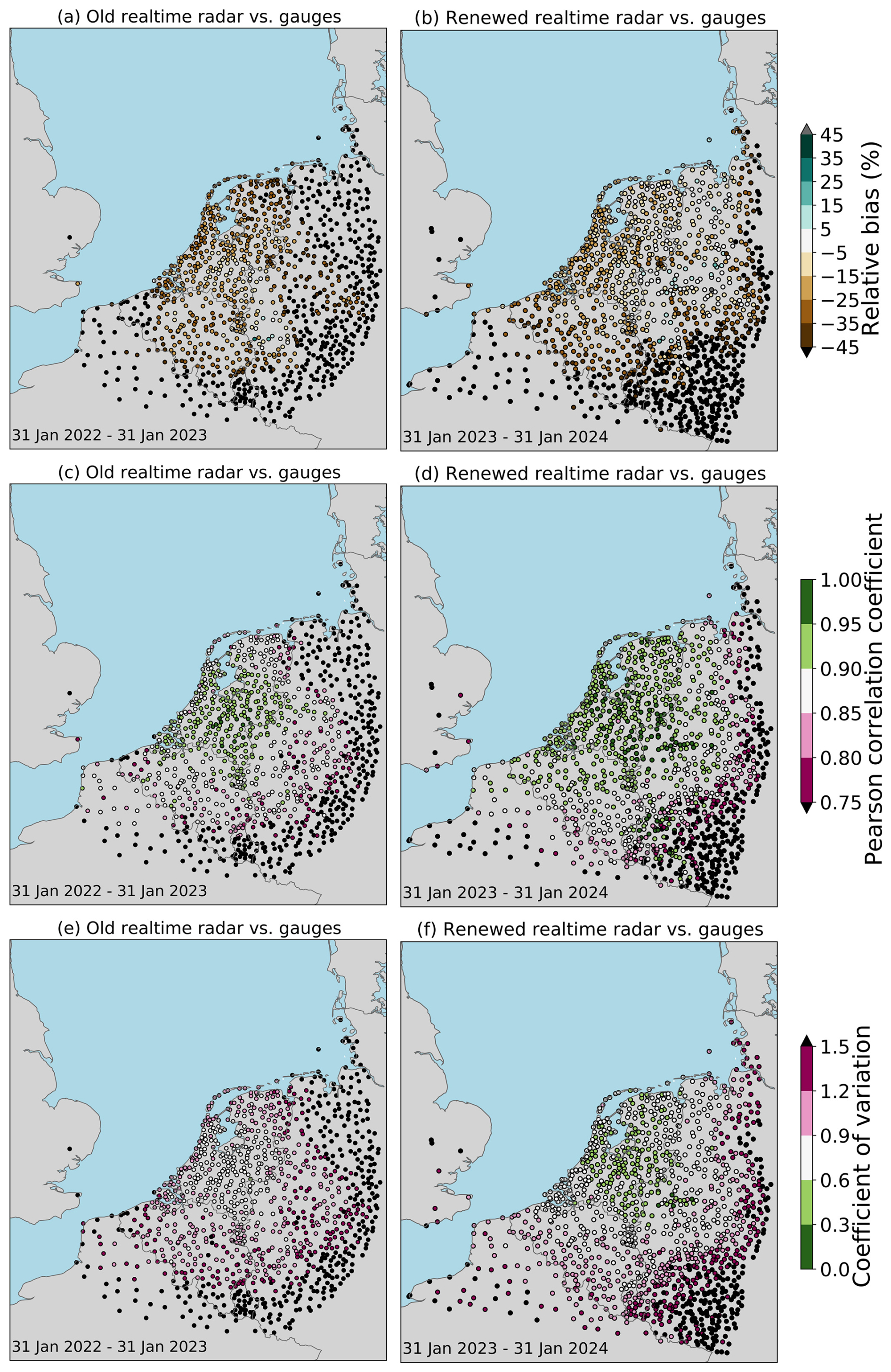
Figure 7 An independent spatial evaluation of the daily radar precipitation accumulations against the daily rain gauge precipitation accumulations for (a, c, e) the old radar product (1008 gauge locations) and for (b, d, f) the renewed radar product (1210 gauge locations). Note that the joint radar–gauge availability is lower for some locations (Fig. 1a and b). Made with Natural Earth.

Compared to the old radar product, the values for ρ generally increase (Fig. 7c and d) and the values for CV generally decrease for the renewed radar product (Fig. 7e and f), confirming the improved performance for precipitation estimation. For the old radar product, values for ρ are typically 0.8 or higher for the land surface of the Netherlands, but rapidly decrease outside the Netherlands to values below 0.75. For the renewed radar product, values for ρ are generally 0.9 or higher for the land surface of the Netherlands, and this is even found for regions in Belgium and Germany that are close to the Dutch border. At farther distances from the Dutch border, values decrease to values below 0.75. Similar behavior is found for the CV. To conclude, the quality of the renewed radar product is much better for the land surface of the Netherlands and Belgian and German regions close to the Dutch border.

4.6 Extremes

The results shown so far are based on all available data, i.e., without thresholding. Here, the quality of the radar precipitation accumulations for a range of rain gauge precipitation threshold values is examined. Figs. 8 and 9 show the values for the relative bias, ρ, and CV, and the number of radar–gauge pairs as a function of this threshold value (step size of 1 mm) for both products for 1 h accumulations and daily accumulations, respectively.

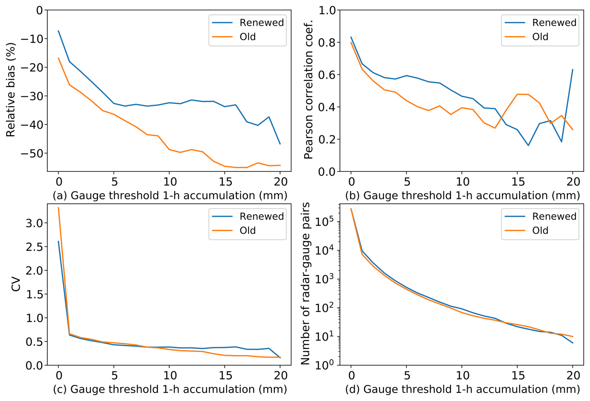
Figure 8 An independent evaluation of 1 h radar precipitation accumulations against the 32 KNMI automatic rain gauge accumulations from the Netherlands for the old (orange lines) and renewed (blue lines) radar product for gauge threshold values ranging from 0 mm (no thresholding) to 20 mm.

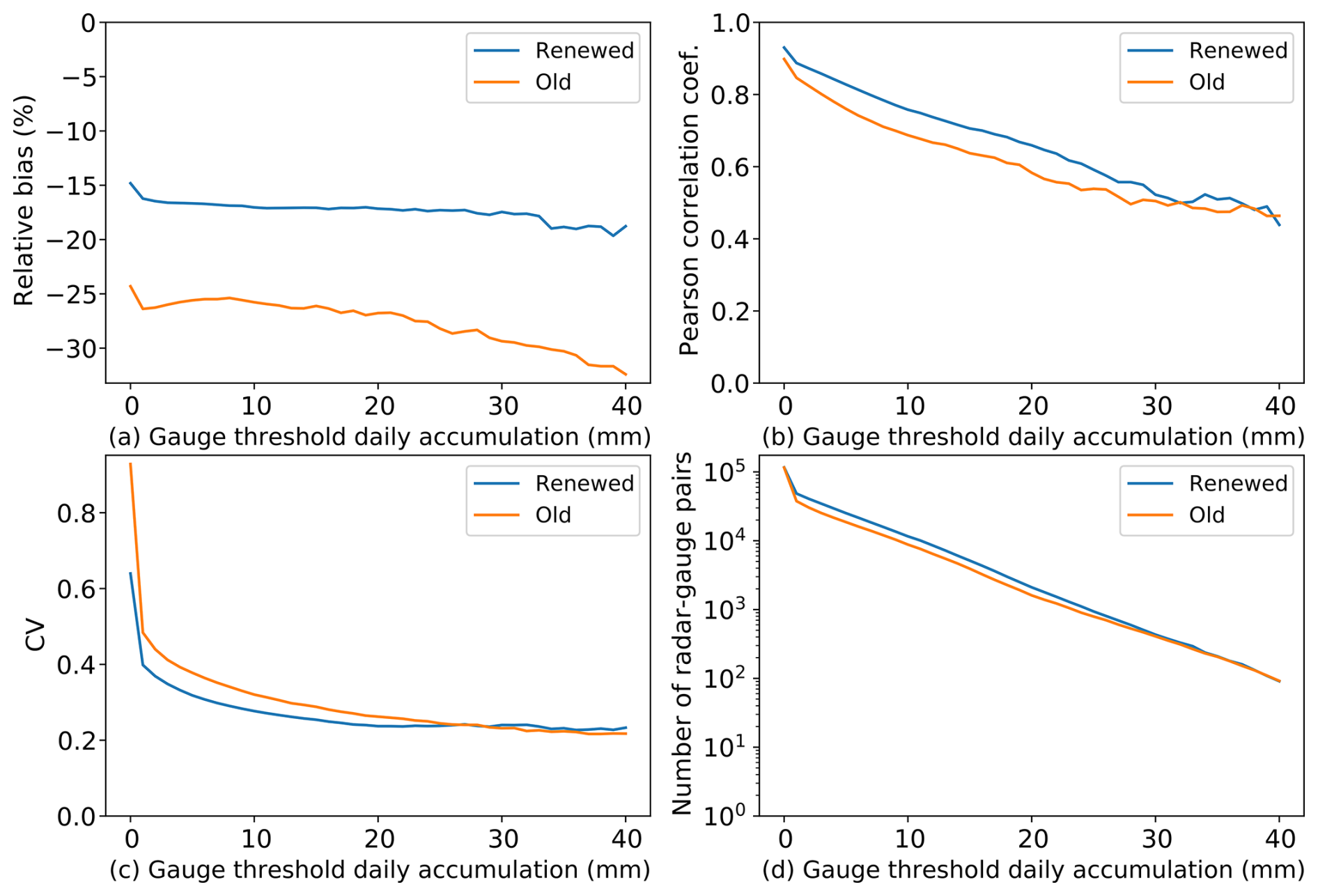
Figure 9 An independent evaluation of the daily radar precipitation accumulations against the 317–319 KNMI manual rain gauge accumulations from the Netherlands for the old (orange lines) and renewed (blue lines) radar product for gauge threshold values ranging from 0 mm (no thresholding) to 40 mm.

The underestimation becomes generally larger for increasing gauge threshold values, but is less severe for the renewed radar product and fairly constant in the 5–15 mm threshold range (Fig. 8a) or the entire threshold range (Fig. 9a) for the renewed product. This is possibly caused by the attenuation correction. Underestimation is only fairly constant for the old product for daily threshold values up to ∼20 mm. The value for ρ usually decreases with increasing threshold value, with the renewed product performing best (Figs. 8b and 9b), except for 1 h threshold values above ∼13 mm, for which erratic behavior is found, likely related to the small sample size (Fig. 8d). The value for CV only strongly decreases from 0 to 1 mm, and remains fairly stable for larger threshold values. Performance is similar for the old and renewed radar products for 1 h threshold values ranging from 0 to ∼10 mm, and slightly better performance for the old product for threshold values larger than ∼10 mm (Fig. 8c). For higher gauge threshold values, the old product outperforms the renewed product. This is possibly related to the fact that both products cover a different 1-year period. In contrast, for daily accumulations, the value for the CV generally decreases with better performance for the renewed product for threshold values ranging from 0 to ∼25 mm, and similar or slightly better performance for the old radar product for the larger threshold values (Fig. 9c). Finally, the number of radar–gauge pairs is generally (slightly) higher for the renewed product and comparable or lower for the highest threshold values (Figs. 8d and 9d).

To summarize, for the renewed radar product the underestimation is approximately 5–20 percentage points less than for the old radar product for the full range of 1 and 24 h threshold values. The values for ρ are (slightly) higher up to the more extreme 1 or 24 h threshold values for the renewed product. The values for CV are equal (1 h) or lower (24 h) up to the more extreme threshold values and become higher (1 h) or equal (24 h) for the most extreme threshold values for the renewed radar product.

4.7 Seasonal dependence

To study a possible seasonal dependence of the quality of radar precipitation accumulations, Fig. 10 shows scatter density plots of the daily accumulations (see also Fig. 5c and d) for 5-month winter (November–March) and summer (May–September) periods. The following conclusions are drawn:

• The precipitation underestimation is clearly higher in the winter period compared to the summer period, with a much larger difference of ∼15 percentage points for the old radar product compared to the ∼8 percentage points for the renewed radar product (Fig. 10).

• For both products, in the summer period, the values for ρ are (slightly) worse and the values for CV are worse compared to the values for the winter period, which may be related to the expected larger representativeness errors between radars and gauges in case of more local, convective rainfall.

• Improvements in the relative bias, ρ², and KGE for the renewed radar product with respect to the old radar product are more pronounced in the winter period. This may indicate the effectiveness of the VPR correction and the fact that the renewed product uses data from closer to the ground, partly due to more radars, and especially close to a radar.

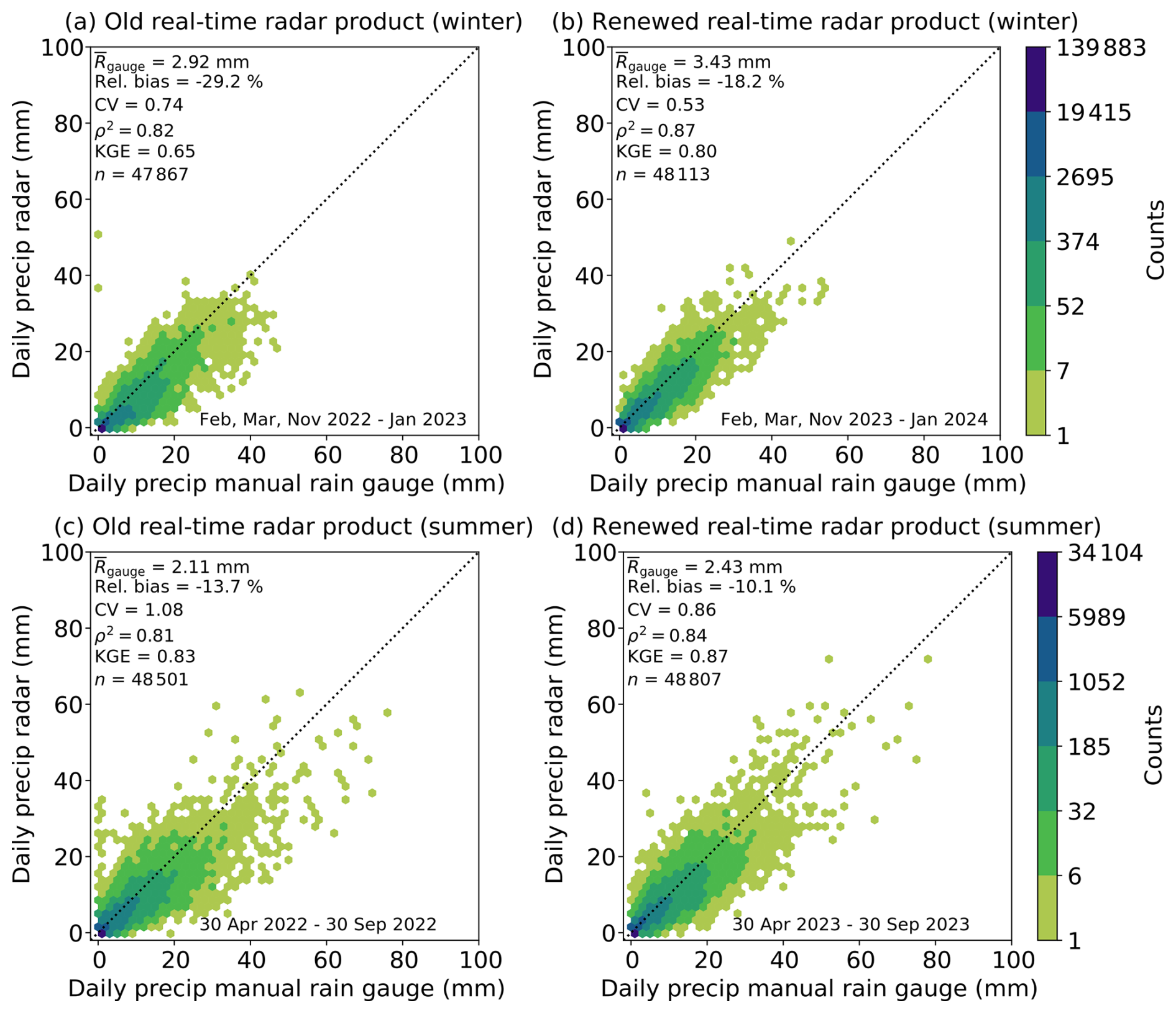
Figure 10 Scatter density plots of the daily radar precipitation accumulations against the independent manual KNMI rain gauge accumulations from the Netherlands for the old (left panels a, c) and the renewed (right panels b, d) radar product for (a, b) the winter period and for (c, d) the summer period.

5 Discussion

The 1-year evaluation periods for the old and renewed radar products do not overlap. Hence, different environmental conditions and precipitation characteristics between those years may also have influenced the comparison between the old and renewed radar products. It is assumed that the effect of this is relatively minor for most of the comparisons presented in this paper because of the lengths of the periods and the resulting large number of samples. The largest effect of using different periods is expected to be on the performance statistics of more extreme precipitation as presented in Figs. 8 and 9. This holds especially for high precipitation thresholds, as these are associated with a much lower number of samples (see panels d of these figures).

The latency of the rain gauge data currently prohibits adjustment of the radar data with gauge accumulations from the same time interval (see Sect. 3.9). Computing a spatial adjustment factor field on past data is not uncommon and useful (Park et al., 2019; Imhoff et al., 2021), and may be the best option. However, this not only results in a less representative adjustment factor field for the current 5 min time interval, but can also cause a sudden change in the 5 min radar precipitation accumulations due to the change of adjustment factor field once an hour (instead of a more gradual change when the adjustment factor field would be computed every 5 min). This is clearly visible in the Supplement (Movie S1) for 04:50–04:55, 05:50–05:55, and 06:50–06:55 UTC. The advantage of the fact that both products use slightly older rain gauge data for this study is that comparisons of the products against 1 h automatic gauge data are fully independent.

An obvious improvement to the QPE product would be to apply real-time gauge accumulations for the adjustment instead of delayed gauge data as is the case for the renewed product. This potential improvement is assessed by rerunning the adjustment for the renewed radar product. For this experiment, the spatial adjustment factor field is computed and applied based on the unadjusted 1 h radar accumulations from the same hour. This mimics the quality of a product for which gauge accumulations without latency would have been available for adjustment. Assessing the resulting daily accumulations leads to an overall improvement with respect to the renewed radar product (Fig. 5d): less underestimation (∼12 % versus ∼15 %), higher values for ρ² (0.90 versus 0.86), lower values for CV (0.56 versus 0.64), and hence higher values for the KGE (0.87 versus 0.83).

There are several remaining (spatially variable) sources of error that have not been corrected for, such as wet radome attenuation (Germann, 1999; Kurri and Huuskonen, 2008), beam blockage, hardware calibration errors (Frech et al., 2017), and assuming a fixed Z_h–R relationship (Marshall et al., 1955; Uijlenhoet, 2001, 2008). These, and the fact that the assumptions underlying the correction algorithms that have been applied are not always valid, contribute to deviations (also spatially variable) found in the radar precipitation product. The relatively low network density of automatic rain gauges employed in the adjustment and the fact that no gauge data are employed outside the Netherlands limit the effectiveness to counteract these sources of error. The use of the threshold T in the radar–gauge adjustment (Appendix B) is meant to prevent small absolute differences in radar or gauge accumulations leading to large differences in the spatial adjustment factor field. However, this may also lead to less or no adjustment for low radar precipitation accumulations, hence not compensating for underestimation. So, for regions and intervals where the precipitation is not captured by the relatively small number of gauges, the precipitation underestimation by the radar cannot be compensated for. Developments and recommendations to address the sources of error in the real-time radar precipitation product are provided in Sect. 7.2.

Since the evaluation is performed against rain gauges, part of the differences can also be attributed to representativeness errors between radars measuring aloft in a large volume (typically ∼1 km³) and gauges measuring locally at the Earth's surface (Kitchen and Blackall, 1992) with a catchment area of typically only ∼500 cm². This is especially true for short durations (e.g., 1 h) where the limited time integration provides only limited compensation for the differences in volumes. Another part of the differences between the radar and gauges is caused by the sources of error in the gauge precipitation estimation (WMO, 2023).

6 Data availability

The 5 min real-time precipitation radar dataset is available from the KNMI Data Platform at https://doi.org/10.21944/5c23-p429 (real time) and https://doi.org/10.21944/e7zx-8a17 (archive) (KNMI Radar Team, 2018a, b) in KNMI HDF5 format containing metadata, such as geographical information (Mathijssen et al., 2019). The data are provided in real time, with one file every 5 min. In this study, the archive has been accessed, which provides a tar file for each day. The data are in UTC. Object “/image1/image_data” contains the 5 min precipitation accumulation (mm). For the renewed radar product, two additional objects are available: object “/image2/image_data” contains the quality index, and object “/image3/image_data” contains the adjustment factor field (dB). Note that “/imageN_data” objects are scaled, which can be found in the metadata (“/imageN/calibration/calibration_formulas”). For instance, the precipitation accumulations need to be multiplied by 100 to obtain the precipitation in millimeters since they are stored as integers in hundredths of millimeters (0.01 mm resolution). The “/image1/calibration_out_of_image” value in “image1/image_data” is used to denote areas outside the radar product domain for that particular time interval, i.e., a “nodata” value (areas void of data).

7 Conclusions and outlook

7.1 Conclusions

The Dutch real-time gauge-adjusted radar QPE product has been available since 19 December 2018 and provides 5 min accumulations every 5 min on a ∼1 km² grid covering the Netherlands and the area around it. Major changes in processing became operational on 31 January 2023, such as clutter removal through a fuzzy logic algorithm (Overeem et al., 2020) and rain-induced attenuation correction (Overeem et al., 2021) on Belgian and Dutch radar data, VPR correction (Hazenberg et al., 2013) on all radar data, quality-based merging of radar reflectivities from different scans and radars, and a spatially variable instead of a mean-field bias adjustment with rain gauge accumulations. The last year of the old dataset and the first year of the renewed dataset were evaluated.

For the renewed radar product, clutter that was present in the old radar product is effectively removed, showing the efficient application of the fuzzy logic clutter algorithm on Belgian and Dutch volumetric radar data and of the Gabella clutter filter on 2D Cartesian data per radar. Applying additional algorithms, such as a satellite cloud (type) mask and a static clutter mask (Saltikoff et al., 2019; Overeem et al., 2023a), do not seem to be necessary.

The influence of beam blockage due to obstacles and orography is also apparent in maps of annual accumulations, exceedance probabilities, and metrics at gauge locations. A beam-blockage correction algorithm (Bech et al., 2003; Krajewski et al., 2006; Lang et al., 2009; Zhang et al., 2013; Cremonini et al., 2016) will likely lead to further improvements of the product.

The evaluation against independent daily rain gauge accumulations generally reveals a clear improvement for the renewed radar product in terms of the relative bias over the Netherlands (10 percentage points less underestimation), Pearson correlation coefficient, and CV. Improvements are also found far away from gauges that are used in the adjustment, likely pointing to the added value of the VPR correction, rain-induced attenuation correction, quality-based compositing, and the use of more low-level data, as well as to the contribution of data from an additional German radar. At the same time, the need for incorporating rain gauge accumulations outside the Netherlands is clear.

Generally, extremes are better captured by the renewed radar product over the Netherlands: underestimations are lower and Pearson correlation coefficient values are higher. Extremes are very important for many of the applications that use radar-based QPE, so this is an especially encouraging result. Precipitation underestimation is stronger in the winter period than in the summer period for both products. Quality improvement in the renewed radar product with respect to the old radar product is strongest in the winter period. This is likely due to the VPR correction and the fact that the quality-based merging algorithm results in using more low-level data.

The importance of the real-time radar precipitation product expands beyond (near) real-time applications, since it forms the basis for the early and final reanalysis products after reprocessing. These two products have a longer latency of ∼1 d and a few weeks, respectively, but their accuracy is higher, since they are enriched with daily manual rain gauge accumulations. Archives of real-time radar precipitation products can also be useful for training and evaluating (machine learning) nowcasting algorithms. The KNMI gauge-adjusted real-time precipitation product is updated every 5 min and is the input for the pySTEPS deterministic nowcasting product (KNMI Radar Team, 2024) and will be used for an upcoming seamless ensemble forecasting product. Hence, any improvements in this precipitation product directly lead to improved nowcasts, forecasts, and early warnings.

7.2 Product outlook

Continuous efforts are needed to further improve the real-time radar precipitation product. The KNMI Radar Team consists of both software developers and researchers, and has adopted the Agile way of working (Agile Alliance, 2025). This allows for fast deployment of improvements to algorithms and addition of new data sources. This makes this real-time QPE product a living dataset. The research carried out on product improvement and evaluation is done in a shared environment, which greatly facilitates collaboration within the team. End users are requested to provide us with feedback on the quality of our product for their specific use case (radar@knmi.nl).

The evaluation of the renewed radar product is assumed to be representative for the current radar product, although already some changes or improvements have been implemented in the renewed radar product after the end of the evaluation period (31 January 2024):

• Data from the German radar in Neuheilenbach have been added since 9 September 2024, providing better coverage (Fig. 1a).

• The latency of the product has been reduced from on average ∼7 to ∼2 min since 9 September 2024. Here, the latency is the time between the end of the last scan and dissemination in the public KNMI Data Platform.

• The forecasted freezing-level height that is employed for the attenuation correction is being taken from ECMWF instead of HARMONIE as of 9 September 2024.

• For the Belgian radar in Jabbeke and the German radars, data from (almost) twice as many elevation scans have been added as of 9 September 2024 and a few more for all Belgian and German radars as of 5 November 2024.

• For the adjustment, a dataset of KNMI automatic rain gauge accumulations has been employed with a much shorter latency of 5–10 min as of 9 October 2024. This results in a 60 min spatial adjustment factor field being computed every 5 min with a latency of 5–10 min. Hence, the adjustment factor field is much more representative for the current 5 min time interval to which it is applied. An estimate of the resulting improvement is provided in Sect. 5.

• The beam blockage in the easterly direction from the Dutch radar in Herwijnen is partly corrected for by assigning a low(er) weight to the data from the blocked sector in the two lowest elevation scans since 5 November 2024. Data from other scans and radars will therefore dominate in the final product, hence greatly reducing the effect of the beam blockage.

• Rain gauge accumulations from ∼150 water authority rain gauges have been subjected to quality control (Van Andel, 2021) and used in the computation of the spatial adjustment factor field since 18 November 2024. Their distribution over the land surface of the Netherlands is irregular, although the coverage is expected to increase. Currently, these gauges receive a low weight in computing the adjustment factor field to prevent overwhelming KNMI's 32 automatic gauges. The weighting and added value of the water authority gauges is still under investigation.

• Improved drizzle detection by avoiding rounding between processing steps was implemented on 24 February 2025.

• We have implemented a cap of ±10 dB on the spatial adjustment factor since 24 February 2025.

In addition, recent (ongoing) research to show the potential for improving the real-time radar precipitation product includes the following:

• Use the differential phase shift to improve precipitation estimation (Testud et al., 2000; Ryzhkov et al., 2014).

• Assess the potential added value of crowdsourced rain gauge accumulations from personal weather stations for the adjustment of radar accumulations. This has already been demonstrated at the European scale (Overeem et al., 2024a) and for the Dutch real-time precipitation product (Svatoš, 2025) for 1 h accumulations from 1 year. These data are potentially available in real time and typically have a much higher network density than government gauges in regions covered by weather radars (Overeem et al., 2024b). This connects to the rise of opportunistic precipitation sensing, as stimulated by the COST Action OpenSense (https://opensenseaction.eu/, last access: 23 January 2025).

Future potential developments are as follows:

• Beam-blockage correction employing a digital elevation model. Blocked sectors from the affected elevation scan are assigned a lower weight. Rainfall retrieval through the differential phase can also help to further mitigate beam blockage, although it still does not sample the blocked part of the measurement volume.

• Improve radar hardware monitoring including alerting.

• Use rain gauge accumulations from Belgian and German (hydro)meteorological services for the adjustment. This is expected to give a major improvement outside the Netherlands, but requires low latency of gauge observations.

• Reduce the latency of KNMI's automatic rain gauge data enabling the computation of a true spatial adjustment factor field that incorporates the last 5 min radar precipitation accumulations.

• Employ hydrometeor classification (Al-Sakka et al., 2013) to further improve precipitation retrieval by conversion to a liquid water content (Smith, 1984; Bukovčić et al., 2018).

• Use Z−R relations specific for the precipitation types (stratiform, convective, undefined; as defined in the VPR correction algorithm).

• Improve the quality index that is contained in the product. This quality index field ranges from 0–1 and serves as a proxy for uncertainty in the precipitation estimates. Optimizing the parameter settings and relationships for the computation of the quality index may yield better estimates of precipitation and its uncertainty. This especially concerns the gauge adjustment, that currently results in quality indices nearing one in the product, which seems not realistic.

• Evaluate other gauge-adjustment methods (Goudenhoofdt and Delobbe, 2009; Winterrath et al., 2012; McKee and Binns, 2015; Barton et al., 2019; De Baar et al., 2023; Nielsen et al., 2024; DWD, 2025).

Appendix A: Computation of the quality index

The quality of radar data is estimated for each radar voxel from individual scans. This quality information is applied in three processing steps:

• Construction of Cartesian maps of surface reflectivity from all scans of a given radar.

• Quality-based compositing when combining these maps from all radars.

• Quality-based weighting of radar–gauge pairs in the gauge adjustment of radar precipitation accumulations.

The procedure to estimate data quality is based on the premise that each correction algorithm is implicitly also a quality assessment. So every source of error, correction, or uncertainty reduces the quality of the radar data. This quality reduction factor Q_X (X is an indicator of the correction algorithm) ranges from 0 (not useful: the resulting quality is 0) to 1 (very useful: no quality reduction). Q_X is computed for the following correction algorithms:

• Clutter identification by Clutter Correction (CCOR) thresholding (based on the amount of Doppler clutter filtering), the fuzzy logic algorithm, and the Gabella clutter filter. If any of these algorithms label a voxel or pixel as clutter, the corresponding quality is set to 0. If a voxel is not labeled as clutter, the amount of reflectivity correction by the Doppler clutter filter (C (dB)) leads to the following quality reduction:

  $$\begin{array}{}\text{(A1)}& Q_{\mathrm{C}}=\exp \left(-\ln \left(\mathrm{2}\right){\left({\displaystyle \frac{\left|C\right|}{C_{\mathrm{0}}}}\right)}^{\mathrm{2}}\right),\end{array}$$

  with C₀ a constant describing the amount of correction associated with halving the quality, here taken as C₀=3 dB.

• Quality reduction in case of higher probability on clutter (F). The fuzzy logic algorithm generates a score F with a probability that the echo in a given voxel is meteorological (i.e., the weighted average of the degree of membership to the meteorological target class). The fuzzy logic algorithm removes voxels with a score lower than 0.6 (Dutch radars) or 0.3 (Belgian radars). This score is employed to compute a quality reduction for the Belgian and Dutch radar data in case the voxel has not been identified as clutter:

  $$\begin{array}{}\text{(A2)}& Q_{\mathrm{F}}=S(F,F_{\mathrm{5}},F_{\mathrm{95}}),\end{array}$$

  where the constants F₅ and F₉₅ show at which point the quality is 0.05 and 0.95, respectively. Here, F₅=0.8 and F₉₅=0.95. The function S is a sigmoid function given by

  $$\begin{array}{}\text{(A3)}& S(x,x_{\mathrm{5}},x_{\mathrm{95}})={\displaystyle \frac{\mathrm{1}}{\mathrm{1}+\exp \left(\frac{\mathrm{2}\log \left(\frac{\mathrm{0.95}}{\mathrm{0.05}}\right)\left(x-\frac{x_{\mathrm{5}}+x_{\mathrm{95}}}{\mathrm{2}}\right)}{x_{\mathrm{5}}-x_{\mathrm{95}}}\right)}}.\end{array}$$

• Quality reduction by the amount of correction for rain-induced path attenuation that has been applied (A). The uncertainty as a result of the correction for attenuation is proportional to the amount of correction A (Overeem et al., 2021). This quality reduction (Q_A) is computed by

  $$\begin{array}{}\text{(A4)}& Q_{\mathrm{A}}=\exp \left(-\ln \left(\mathrm{2}\right){\left({\displaystyle \frac{\left|A\right|}{A_{\mathrm{0}}}}\right)}^{\mathrm{2}}\right),\end{array}$$

  with A₀ a constant describing the amount of correction associated with halving the quality, here A₀=3 dB.

• Quality reduction by the amount of correction for the VPR that has been applied (V). This quality reduction Q_V has the same form as the quality reduction by the Doppler clutter filter (Eq. A1) and attenuation correction (Eq. A4). Again, halving the quality corresponds to a 3 dB correction.

• Quality reduction by uncertainty in the derived VPR (U). The estimation of the VPR comes with an uncertainty estimate. This uncertainty also results in a quality reduction Q_U that is computed in the same manner as in Eqs. (A1) and (A4), where halving the quality again corresponds to 3 dB uncertainty.

• Quality reduction as a result of the height of the sampling volume above the Earth's surface (H). The higher the sampling volume, the more can happen with the precipitation before it reaches the Earth's surface. This is already partly taken into account by the VPR correction for stratiform and undefined precipitation, but the uncertainty will increase with the height due to greater differences between the precipitation aloft and on the ground (both hydrometeor type and size distributions). In addition, despite the application of algorithms to remove clutter, residual ground clutter could still be present. Hence, the quality close to the Earth's surface is also considered low, but rising steeply in the lower 500 m of the atmosphere. The resulting quality reduction Q_H as a function of height h is computed by

  $$\begin{array}{}\text{(A5)}& Q_{\mathrm{H}}={\displaystyle \frac{S(h,\mathrm{0},h_{\mathrm{l}})-\mathrm{0.05}}{\mathrm{0.95}}}S(h,h_{\mathrm{h}},h_{\mathrm{m}}),\end{array}$$

  where $\mathrm{0}<h_{\mathrm{l}}<h_{\mathrm{m}}<h_{\mathrm{h}}$. So the quality first increases from the ground to h_l=0.5 km, followed by a stable high quality (∼0.95) up to h_m=1.0 km, after which it decreases again to a value of approximately 0.05 at h_h=4.0 km. Again, the function S is the sigmoid function (Eq. A3).

• Quality reduction as a result of the distance to the radar (R). The further away from the radar, the larger the sampling volume over which the precipitation is averaged (beam broadening). The resulting quality reduction (Q_Rm) as a function of distance r (km) to the radar is assumed to be linear:

  $$\begin{array}{}\text{(A6)}& Q_{\text{Rm}}=\left\{\begin{array}{ll}\mathrm{1}-\frac{r}{r_{\mathrm{m}}}& \text{if}r<r_{\mathrm{m}}\\ \mathrm{0}& \text{if}r\ge r_{\mathrm{m}},\end{array}\right.\end{array}$$

  with r_m the distance (km) at which the quality is reduced to 0. Here, r_m=500 km. To avoid sharp discontinuities at the maximum range of a radar scan, the quality is reduced (Q_Re) in the last r_e km of the scan:

  $$\begin{array}{}\text{(A7)}& Q_{\text{Re}}=\left\{\begin{array}{ll}\mathrm{1}& \text{if}r\le r_{\text{max}}-r_{\mathrm{e}}\\ \mathrm{1}-{\left(\frac{r-r_{\text{max}}}{r_{\mathrm{e}}}+\mathrm{1}\right)}^{\mathrm{2}}& \text{if}r>r_{\text{max}}-r_{\mathrm{e}},\end{array}\right.\end{array}$$

  with r_max the maximum possible distance to the radar for the chosen scan. This reduction is applied to the last r_e=50 km of the scan. The total quality reduction (Q_R) as a consequence of the distance to the radar is then

  $$\begin{array}{}\text{(A8)}& Q_{\mathrm{R}}=Q_{\text{Rm}}\cdot Q_{\text{Re}}.\end{array}$$

The total quality index Q_T is the product of all quality reduction factors described above:

$$\begin{array}{}\text{(A9)}& Q_{\mathrm{T}}=Q_{\mathrm{C}}\cdot Q_{\mathrm{F}}\cdot Q_{\mathrm{A}}\cdot Q_{\mathrm{V}}\cdot Q_{\mathrm{U}}\cdot Q_{\mathrm{H}}\cdot Q_{\mathrm{R}}.\end{array}$$

Appendix B: Computation and application of the spatial adjustment factor field

This appendix follows the procedure as described in Overeem et al. (2023a), but with some modifications regarding the settings. The spatial adjustment factor field F_adj is calculated as follows for each radar pixel i with position (x_i,y_i):

$$\begin{array}{}\text{(B1)}& F_{\text{adj}}(x_i,y_i)=\left\{\begin{array}{ll}\frac{S_{\text{w,r}}}{S_{\text{w,g}}}& \text{if}{S}_{\text{w,r}}>T\bigvee S_{\text{w,g}}>T,\\ \frac{T}{S_{\text{w,g}}}& \text{if}{S}_{\text{w,r}}\le T\bigvee S_{\text{w,g}}>T,\\ \frac{S_{\text{w,r}}}{T}& \text{if}{S}_{\text{w,r}}>T\bigvee S_{\text{w,g}}\le T,\\ \mathrm{1}& \text{if}{S}_{\text{w,r}}\le T\bigvee S_{\text{w,g}}\le T,\end{array}\right.\end{array}$$

with T a threshold value of 0.25 mm. The distance-weighted sum of 60 min precipitation accumulations at gauge locations is denoted by S_w,X, with X an indicator being g (gauge) or r (radar):

$$\begin{array}{}\text{(B2)}& S_{\text{w},X}=\sum _{n=\mathrm{1}}^{N_{\mathrm{p}}}{w}_n{R}_{X,n},\end{array}$$

which is calculated over N_P radar–gauge pairs, with the 60 min precipitation accumulation for the gauge at location n denoted by R_g,n and the corresponding accumulation for the unadjusted radar data denoted by R_r,n.

In the case of low precipitation accumulations, the values for S_w,X may be very sensitive to errors in both radar and gauge estimates, leading to very uncertain adjustment factors. Especially in cases where radar accumulations are significant at other locations than at the gauges, the absolute effect on the resulting precipitation field may be large. For example, in the case of underestimation by the radar, this may lead to unrealistic extreme accumulations in the final product. To prevent this, the value of S_w,X is set equal to T when it becomes smaller than T (see Eq. B1).

The weighting function w_n is a function of the distance of a pixel to a gauge location n and of the quality of radar and rain gauge data:

$$\begin{array}{}\text{(B3)}& w_n={\displaystyle \frac{G_{\mathrm{w}}\left(n,r_{\mathrm{s}}\right)+v\cdot G_{\mathrm{w}}(n,r_{\mathrm{l}})}{\mathrm{1}+v}}{Q}_{\mathrm{r},n}{Q}_{\mathrm{g},n},\end{array}$$

where G_w(n,r_d) is a Gaussian function:

$$\begin{array}{}\text{(B4)}& G_{\mathrm{w}}(n,r_{\mathrm{d}})=\left\{\begin{array}{ll}\frac{\exp (-\mathrm{4}\frac{{\mathit{\delta }}_{i,n}^{\mathrm{2}}}{r_{\mathrm{d}}^{\mathrm{2}}})-\exp (-\mathrm{4})}{\mathrm{1}-\exp (-\mathrm{4})}& \text{if}{\mathit{\delta }}_{i,n}^{\mathrm{2}}\le r_{\mathrm{d}},\\ \mathrm{0}& \text{if}{\mathit{\delta }}_{i,n}^{\mathrm{2}}>r_{\mathrm{d}},\end{array}\right.\end{array}$$

in which ${\mathit{\delta }}_{i,n}=\sqrt{(x_i-x_n{)}^{\mathrm{2}}+(y_i-y_n{)}^{\mathrm{2}}}$ is the distance between the gauge and the radar pixel, and (x_n,y_n) is the position of gauge n. Note that the quality of both gauge data (Q_g,n) and radar data (Q_r,n; see Appendix A) is taken into account. In the current implementation, the quality of the rain gauge data is set to a fixed value of 0.9 (assumed quality due to measurement and representativeness errors). If the gauge quality differs across the network, this algorithm is hence able to take that into account. The weighting consists of a short-range and a long-range component, each having its own Gaussian function in Eq. (B3). The Gaussian function decreases to 0 when a pixel is located at a range of at least r_d km from the selected gauge location n. The long-range component contributes up to a range of 500 km (r_l) and is meant for adjusting when the distance to the nearest gauges is long, typically further away from the Netherlands. The short-range component provides a much more local adjustment up to a range of r_s, which is based on the range of a seasonally-dependent isotropic spherical variogram model of rainfall accumulations corresponding to a 1 h duration (Van de Beek et al., 2012). The value of v controls the contribution of the long-range component with respect to the short-range component, and is set to v=0.1 in the current implementation.

The real-time radar precipitation product of 5 min accumulation (R_r,adj; mm) at a radar pixel i with position (x_i,y_i) is obtained as follows:

$$\begin{array}{}\text{(B5)}& R_{\text{r,adj}}(x_i,y_i)={\displaystyle \frac{R_{\mathrm{r}}(x_i,y_i)}{{\mathrm{10}}^{F_{\text{adj}}(x_i,y_i)/\mathrm{10}}}},\end{array}$$

with R_r the 5 min unadjusted accumulation (mm), and F_adj the spatial adjustment factor field (see Eq. B1).

A quality index field (Q) is also computed for each pixel. Each rain gauge measurement that is added to the product should increase the quality, and the resulting quality index should be between 0 and 1. This leads to the following expression for the product quality:

$$\begin{array}{}\text{(B6)}& Q_i=Q_{\mathrm{r},i}\left(\mathrm{1}-\prod _{n=\mathrm{1}}^{N_{\mathrm{p}}}(\mathrm{1}-w_n{Q}_{\mathrm{g},n})\right),\end{array}$$

with Q_r,i the radar quality at pixel i (Eq. 2) and Q_g,n the quality of the observation from rain gauge n.