A 30-month data set of glider physico-chemical data off Mayotte Island near the Fani Maoré volcano

In May 2018, an unprecedented long and intense seismo-volcanic crisis broke out off the island of Mayotte (Indian Ocean) and was associated with the birth of an underwater volcano (Fani Maoré). Since then, an integrated observation network has been created (REVOSIMA), with the objective of monitoring and better understanding underwater volcanic phenomena. Recently, an autonomous ocean glider (ALSEAMAR's SeaExplorer) was deployed to supplement the data obtained during a series of oceanographic surveys (MAYOBS) carried out on an annual basis. Operated by ALSEAMAR in collaboration with IFREMER, the glider performed a continuous monitoring of the water column, from the sea surface to 1250 m water depth, over 30 months between September 2021 and April 2024 with the objective of acquiring hydrological properties, water currents and dissolved gas concentrations. This monitoring showed the feasibility and value of measuring autonomously, continuously and at a high spatio-temporal scale the physical (temperature, salinity, ocean current) and biogeochemical parameters (O₂, CH₄, CO₂, bubbles/droplets, vertical speed anomalies related to droplets) over several months using a glider. In particular, innovating sensing capabilities (e.g. MINICO2, acoustic Doppler current profiler (ADCP)) have shown great potential in the context of the Mayotte seismo-volcanic crisis despite technical challenges (complex algorithms, sensor capabilities, etc.). Data described in this paper can be accessed at the SEANOE repository under DOI: https://doi.org/10.17882/99960 (Heumann et al., 2024).

1 Introduction

Mayotte is a French overseas territory, part of the volcanic archipelago of the Comoros Islands, northwest of Madagascar. It was last volcanically active on land less than 7000 years ago (Zinke et al., 2003, 2005).

On 10 May 2018, a seismo-volcanic crisis of unprecedented intensity and duration began off the two main islands of Grande-Terre and Petite-Terre (Lemoine et al., 2020). More than 11 000 earthquakes were recorded, up to a magnitude of 5.9, in an area where only two seismic events had been recorded since 1972 (Feuillet et al., 2021). At sea, the epicentres of these earthquakes were divided into the proximal area (5 to 15 km east of Petite-Terre) and the distal area (25 km east of Petite-Terre).

Following the start of this seismic crisis on 1 July 2018, surface displacements were measured by the GPS stations present in Mayotte, revealing an eastward displacement of between 21 and 25 cm for all of these stations, as well as a subsidence of between 10 and 19 cm depending on their location (Feuillet et al., 2021).

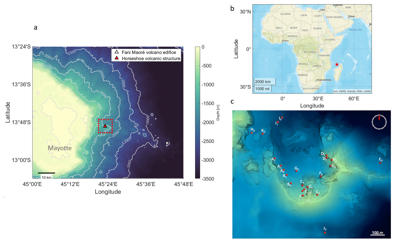
Figure 1 Map view of Mayotte (a); the Fani Maoré volcano edifice is represented by the white triangle which lies 50 km southeast of Mayotte, and the Horseshoe area is represented by the red triangle and the dotted red line located 10 km east of Mayotte. Map view of Africa and the Middle East (b), where the red star is the Mayotte Island. Map illustrating the Horseshoe structure (c). The red dots correspond to the discovered emission sites of magmatic fluid identified with the multibeam echo sounder during the REVOSIMA MAYOBS cruises (https://doi.org/10.12770/070818f6-6520-49e4-bafd-9d4d0609bf7d, Scalabrin, 2023) and validated by in situ visual observations with the remotely operated vehicle (ROV) VICTOR during the GEOFLAMME cruise (https://doi.org/10.17600/18001297, IFREMER, 2021). Bathymetric data were provided at a resolution of 20 m (https://doi.org/10.18142/291, IFREMER, 2025).

In response to this crisis, French laboratories and institutions – Institut de Physique du Globe de Paris (IPGP), Centre National de la Recherche Scientifique (CNRS), Bureau de Recherches Géologiques et Minières (BRGM), Institut Français de Recherche pour l'Exploitation de la Mer (IFREMER), Institut de Physique du Globe de Strasbourg (IPGS) – created a volcanological and seismological monitoring network in Mayotte, the Réseau de surveillance volcanologique et sismologique de Mayotte (REVOSIMA, http://www.ipgp.fr/fr/revosima/acteurs-reseau, last access: 5 August 2024). This observatory, both marine and terrestrial, benefits from the financial support of several ministries (Ministry of Overseas; Ministry of the Interior, Ministry of Higher Education, Research and Innovation; Ministry of Ecological Transition and Solidarity) and aims to further our understanding of the seismo-volcanic activity for preservative measures in order to protect populations. As part of REVOSIMA, several oceanographic cruises have been carried out (MAYOBS cruises, https://doi.org/10.18142/291, IFREMER, 2025), and bulletins monitoring seismo-volcanic activity are published monthly (http://www.ipgp.fr/fr/revosima/actualites-reseau, last access: 9 April 2024). The first oceanographic cruise (MAYOBS1) was carried out from 2 to 18 May 2019 on the RV Marion Dufresne and led to the discovery of the ongoing eruption of the new Fani Maoré submarine volcano. A new volcanic structure of 800 m formed during this crisis, with a height of around 800 m, located 50 km off the coast of Mayotte and at a depth of 3500 m (Feuillet et al., 2021; Aiken et al., 2021, Fig. 1). The estimated volume of magma emitted during this eruptive period is 6.55 km³, ranking this event as the largest submarine volcanic eruption ever documented (Feuillet et al., 2021). Four other ongoing lava flows were revealed during subsequent oceanographic cruises in the nearby area around the new volcano (Feuillet et al, 2021.). During the MAYOBS cruises, the pre-existing Horseshoe volcanic structure, located above the proximal swarm at an average seafloor depth of 1400 m, was a particular area of interest (Fig. 1). Acoustic plumes and geochemical anomalies (elevated concentrations of dissolved gases such as carbon dioxide CO₂, methane CH₄ and dihydrogen H₂) were detected using a multibeam echo sounder and CTD (conductivity, temperature and depth) rosette measurements. These acoustic plumes are detectable in the water column from the seafloor up to around 500 m and are distributed over 23 active emission sites identified to date (Scalabrin, 2023; Fig. 1). The specific magmatic origin of these fluid emissions has yet to be determined (Mastin, 2023).

The ocean circulation around Mayotte Island is mainly influenced by the instabilities of the Northeast Madagascar Current (NEMC), which originates from the splitting of the westward South Equatorial Current (SEC) (Schott et al., 2009). While the anticyclonic eddies, mainly generated to the west of Cape Amber (the northernmost cape of Madagascar), strongly influence the circulation around Mayotte Island, cyclonic eddies formed along the northwestern coast of Madagascar rarely reach the island (Collins et al., 2014). The large-scale circulation is also strongly influenced by seasonally reversing winds linked to the monsoon regimes (Manyilizu et al., 2016).

This highly complex circulation consists of a southward flow coupled with mesoscale eddies (diameter ≥ 300 km) that can affect the entire water column (de Ruijter et al., 2002; Halo et al., 2014). The general circulation in the area is even more complex due to the significant influence of the islands on the local hydrodynamic context.

Significant variability in hydrographic parameters is observed within the upper 1500 m of the water column. This temporal variability spans a broad range of timescales. High-frequency variations (from a few hours to several days) are primarily driven by tidal forcing. At intermediate timescales, fluctuations with a periodicity of 60 to 90 d are associated with the passage of anticyclonic eddies, particularly in the southern part of the study area (Collins et al., 2014). On longer timescales, annual variability is evident and is largely governed by large-scale climatic forcing.

Relatively little reference data are available for the nearby area of Mayotte Island, and so it remains poorly understood. Tide gauges have been installed on the coasts of the main islands, and internal tidal waves have been observed during MAYOBS campaigns.

In order to monitor the dissolved gas dynamics related to volcanic events in the Horseshoe area and as a complement to regular oceanographic cruises, SeaExplorer glider deployments from ALSEAMAR (https://www.alseamar-alcen.com/, last access: 17 August 2024), equipped with biogeochemical sensors, have been carried out since 17 September 2021 with funding from REVOSIMA. These deployments are still carried out up to date to ensure the monitoring of this seismo-volcanic crisis.

The SeaExplorer glider is a member of the family of autonomous underwater drones that can provide continuous collection of high-resolution underwater data between the surface and its maximum depth rating (1250 m) with very wide spatial (several thousand kilometres) and temporal (up to 2 months) coverage. Supervised by an Iridium satellite link, the vehicle enables near-real-time observation and monitoring of the oceans from a control centre on land. The Global Ocean Observing System (GOOS), led by the Intergovernmental Oceanographic Commission (IOC) of UNESCO and co-sponsored by the World Meteorological Organization (WMO), the United Nations Environment Programme (UNEP) and the International Science Council (ISC), has been coordinating national ocean-observing efforts for more than 20 years. In this international effort, the role of autonomous glider observations has always been seen as a way to compensate for the limitations of other observing means (Stommel, 1989). The contribution of gliders began in earnest in the 2010s, when the technology was mature enough to contribute to global observations (Testor et al., 2010). Since 2016, the OceanGliders component of GOOS has also been in charge of the coordination and improvement of the use of gliders around the world.

2 Data and methods

2.1 Mission overview

The glider has been deployed at sea near the eastern coast of Petite-Terre since 17 September 2021 (12 km southwest of the Horseshoe area: 12°53.5^′ S, 45°19^′ E). It is operated for 14 d on average before being recovered at sea to collect the full data set. The glider is then immobilized on land for 1 night to recharge the battery and perform regular maintenance before being redeployed the next day.

In the course of more than 2 and a half years of deployment, six gliders have been used for 72 deployments (see Table A1 in the Appendix).

These gliders are equipped with a CTD (conductivity, temperature, depth) instrument, either a SeaBird GPCTD or an RBR LEGATO. Dissolved oxygen sensors are also deployed, namely an SBE43F from SeaBird coupled with the GPCTD and an AROD-FT from JFE coupled with the LEGATO. These two sets of sensors, while having small technology differences (pumped sensors for SeaBird and unpumped sensors for RBR and JFE), provide comparable data (see Table D1). The scientific payload also includes an 1 MHz acoustic Doppler current profiler (ADCP) from Nortek (Signature1000 ADCP specifications with a casing modified for glider integration), a METS (dissolved methane sensor) from Franatech and a MINICO2 (dissolved CO₂ sensor) from Pro-Oceanus (see Table A1).

To carry out the mission, a specific and unusual sampling strategy was implemented. Until August 2023, the glider was limited to a maximum immersion depth of 1000 m. In order to stay as near as possible to the seafloor, where magmatic fluid emissions occur and should be sampled, the glider's navigation consisted of a three-phase progression: a downward phase where the glider reached a depth of 1000 m; a forward navigation phase, with about 10 ascent–descent phases (i.e. yo) between 900 and 1000 m; and a final phase of ascent to the surface. Dives carried out in the Horseshoe area last on average 8 to 9 h, with 6 h on average being spent between 900 and 1000 m, covering a distance of around 6 km. This radial navigation strategy, consisting of navigation at a fixed heading toward the central point of the Horseshoe structure, enables objective sampling of the zone of interest, covering all of its quadrants equally, with maximum sampling effort at its centre, decreasing progressively with distance (Fig. 2).

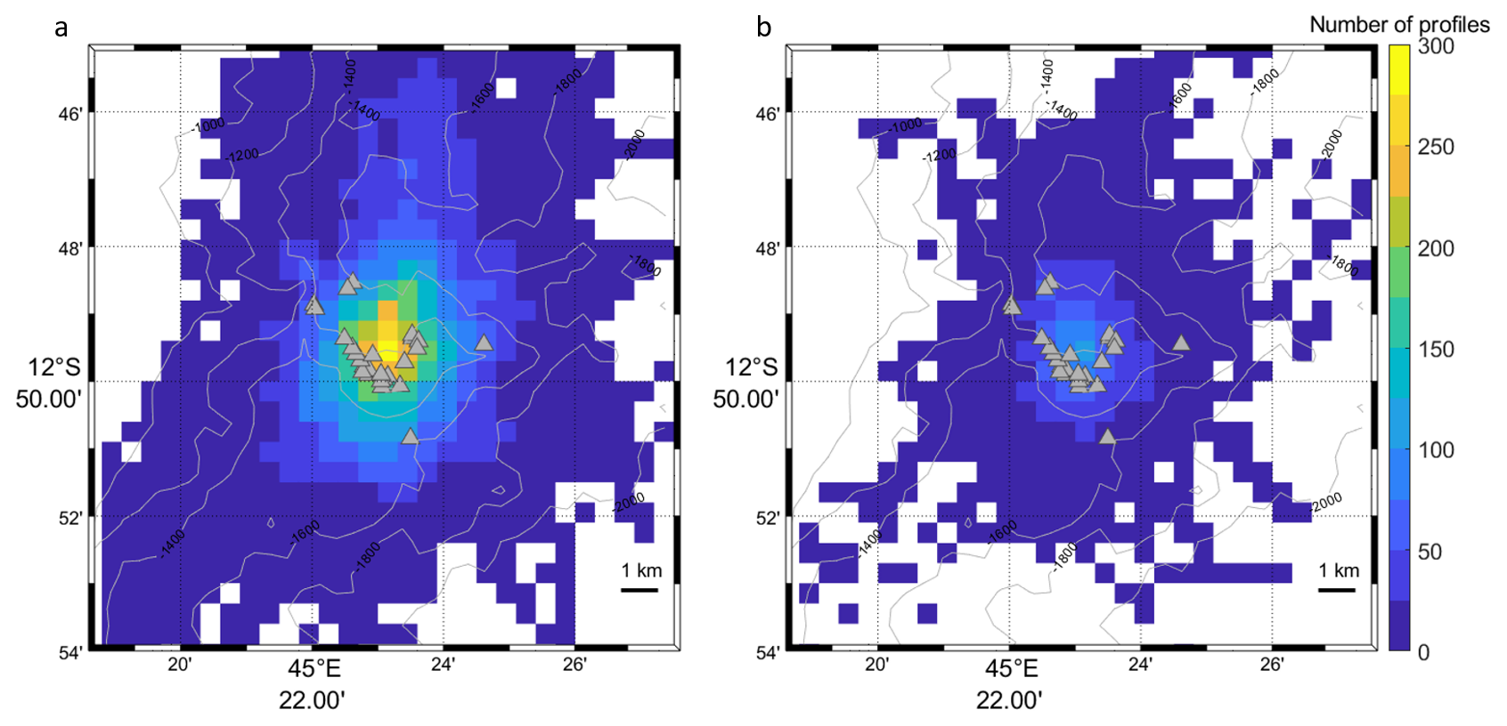
Figure 2 Map illustrating the sampling effort based on the number of profiles acquired with the 1000 m max depth rating of SeaExplorer between September 2021 and August 2023 in rectangles of 0.25 km² (a) and map illustrating the sampling effort based on the number of profiles acquired by the 1250 m max depth rating of SeaExplorer between August 2023 and April 2024 in rectangles of 0.25 km² (b). The triangles are the active fluid emission sites identified with the multibeam echo sounder during the REVOSIMA MAYOBS cruises (https://doi.org/10.12770/070818f6-6520-49e4-bafd-9d4d0609bf7d, Scalabrin, 2023) and validated by in situ visual observations with the ROV VICTOR during the GEOFLAMME cruise (https://doi.org/10.17600/18001297, IFREMER, 2021). Isobaths are processed from GEBCO gridded bathymetry data (https://doi.org/10.5285/1c44ce99-0a0d-5f4f-e063-7086abc0ea0f, GEBCO Bathymetric Compilation Group 2024, 2024).

For the first time, two glider prototypes with a maximum immersion capacity of 1250 m have also been deployed in the area since August 2023. A slightly different navigation method was chosen, opting for spirals instead of straightforward dives. The radius of these spirals is 1.5 km in order to cover the entire study area as nearly as possible over the duration of a deployment.

Initially, a wide mapping of the area was chosen until August 2023 to detect seafloor fluid emissions and to get an idea of the physico-chemical properties over a large area. With this new navigation method, sampling is then focused on better characterization of the active fluid sites (Fig. 2).

These spirals also consist of a downward phase to a depth of 1250 m, followed by several yo's between 800 and 1250 m, and finally an ascent to the surface. These types of dives last an average of 10 h. This sampling method was chosen to ensure a good quality of data from dissolved gas sensors by flushing the sensors (see Sect. 2.2.2 and 2.2.3) and to focus the navigation on known active sites and their immediate surroundings.

The data produced during the continuous acquisition at high sample rates between September 2021 and April 2024 represent a substantial amount (∼2.2 million measuring points per sensor, corresponding to ∼22 000 dives).

2.2 Data processing

The CTD and dissolved gas sensors mounted on the SeaExplorer glider acquire measurements at a frequency of 1 Hz, subsequently averaged into 30 s time series available through the SEANOE data centre (see “Data availability” section). While data are averaged to 30 s intervals, this corresponds to approximately 5 m of vertical resolution at a typical glider ascent or descent speed. To optimize power consumption, the ADCP operates at a lower sampling frequency of 0.1 Hz, with its data similarly being averaged into 30 s intervals. As a result, fine-scale vertical structures or sharp shear zones may be partially smoothed, although the resolution remains adequate for capturing broader vertical patterns of current variability.

2.2.1 CTD and DO data

For processing of the sensor pair GPCTD and SBE43F, the salinity (SAL) is derived from raw conductivity measurements, and the potential density with a reference pressure of 0 dbar is approximated with the 75-term function of temperature (TEMP), salinity and pressure (PRES) (Roquet et al., 2015). Computations were performed according to international standards and using TEOS-10 GOOS standards (http://www.teos-10.org/pubs/IOC-XXV-3_e.pdf, last access: 2 June 2024).

Data processing is carried out in accordance with OceanGliders standard operating procedures (SOPs) (Lopez-Garcia et al., 2022, https://github.com/OceanGlidersCommunity, last access: 28 June 2024). Moreover, the thermal-lag effect was addressed using the methodology described in Garau et al. (2011) for both CTD sensors.

Computation of dissolved oxygen data in physical units was performed following the algorithm of Owens and Millard (1985).

For the sensor pair LEGATO CTD and AROD-FT, the data are processed internally by the sensors. Dissolved oxygen data are directly available in µmol kg⁻¹, while salinity data are also computed from the conductivity data using the same correction algorithm applied to the GPCTD.

O₂ time series acquired with the different sensors used underwent large discontinuities, which were ubiquitously related to instrumental deficiencies. To deal with this issue, the time series was split into discrete segments according to the different sensors operated, all based on OceanGliders SOP (Lopez-Garcia et al., 2022). The assembled proposed adjustments (gains) were applied to make the entire glider time series continuous. Gain values applied for each discontinuity can be found in Table B1. Illustrative examples of profile corrections are presented in Fig. C1. Sensor units, ranges, precisions and resolutions can be found in Table D1.

2.2.2 CO₂ data

The response time of membrane-based sensors is a major constraint for profiling platforms (Fiedler et al., 2013). Although the glider is a rather slow profiling device, with an average vertical speed of about 15 cm s⁻¹, the MINICO2 response time causes an appreciable hysteresis in vertical CO₂ profiles. A time lag correction algorithm (Miloshevich et al., 2004) has been applied on carefully smoothed vertical profiles of CO₂ (to minimize noise amplification caused by the processing algorithm) using the following model, sequentially:

$$\begin{array}{}\text{(1)}& {\mathrm{CO}}_{\mathrm{2},\mathrm{corr}}\left(t\right)={\displaystyle \frac{{\mathrm{CO}}_{\mathrm{2},\mathrm{raw}}\left(t\right)-{\mathrm{CO}}_{\mathrm{2},\mathrm{raw}}(t-\mathrm{1})e^{\frac{-\mathrm{\Delta }t}{\mathit{\tau }}}}{\mathrm{1}-e^{\frac{-\mathrm{\Delta }t}{\mathit{\tau }}}}},\end{array}$$

where CO_2,raw(t) is the measured value at the time t, CO${}_{\mathrm{2},\mathrm{raw}}(t-\mathrm{1})$ is the measured value at the previous time stamp, Δt is the time between two measurements (1 s for raw measurements or 30 s for sub-sampled measurements), CO_2,corr(t) is the time-lag-corrected (TLC) measurement at t, and τ is the response time. Previous studies have shown pronounced changes in τ that linearly depend on water TEMP (Fietzek et al., 2014): the warmer the water, the faster the response time. In the absence of published values for the MINICO2 sensor, the linear relationship was determined empirically, minimizing the difference in CO₂ between upcast and downcast profiles of a dive. Finally, raw CO₂ data recorded in ppm were converted into µmol L⁻¹ based on the manufacturer calculation sheet and using in situ temperature and salinity values measured by the CTD.

2.2.3 CH₄ data

The measurement of CH₄ might be impacted by various external factors such as temperature, in situ CH₄ or the moving speed of the glider. The main consequences are an artificially increasing CH₄ with decreasing temperature, an hysteresis between the upcast and the downcast phases of a profile, and thermal and temporal lags (Meurer et al., 2021; Russell-Cargil et al., 2018).

In the present study, these issues were first addressed by adapting the sampling strategy. Indeed, the glider was programmed to dive deep into multiple yo's to limit the impact of varying environmental conditions. This way, it is expected that temporal changes in CH₄ (e.g. induced by natural seepage) would be more easily detectable compared to a situation where the glider would cross regularly strong temperature gradients. Comparison of CH₄ profiles between upcast and downcast phases enabled the computation of a lag in the sensor response time (τ) of about 6 min. The estimated sensor response time implies that CH₄ measurements are subject to a significant temporal smoothing, particularly during phases of rapid vertical variation such as near inflection points in the profiles. Adjusted CH₄ (CH_4,corr) values were thus calculated following the Meurer et al. (2021) algorithm:

$$\begin{array}{}\text{(2)}& {\mathrm{CH}}_{\mathrm{4},\mathrm{corr}}\left(t\right)={\mathrm{CH}}_{\mathrm{4}}(t+\mathit{\tau }),\end{array}$$

where t is the time, while τ varies according to the sensor used (Table A1). Sensor units, ranges, precisions and resolutions can be found in Table D1.

2.2.4 ADCP data

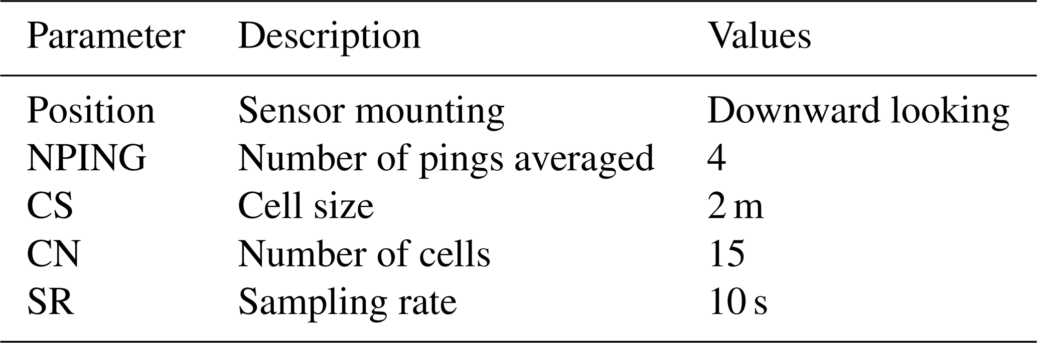
For the purpose of this project, the ADCP was programmed to obtain current profiles with a high resolution. Values of the main tunable parameters can be found in Table 1. The method used to retrieve ocean currents is the “shear method” (Visbeck, 2002) to subtract the unknown motion of the glider from the absolute water velocity calculated by the ADCP.

Table 1 ADCP configuration and processing.

It is worth noting that glider ADCP measurements must undergo several quality control steps before profiles of ocean velocity can be properly estimated. It is a critical issue, and this must be done with great caution. Pasqueron de Formmervault et al. (2018) developed a number of tests specifically adapted for the SeaExplorer glider. As stated in Pasqueron de Formmervault et al. (2018), ocean velocity data retrieved from glider-mounted ADCP show a mean difference of 1.5 cm s⁻¹ compared to reference mooring data. This value corresponds to a simple yo pattern using a SeaExplorer glider. In our case, using repeated multi-yo patterns until August 2023, followed by spiral multi-yo's from August 2023 to April 2024, the uncertainty is likely to be higher than 1.5 cm s⁻¹. Based on our preliminary assessments, it may remain below 10 cm s⁻¹, although this upper bound should be considered with caution.

The quality of the data set was assessed at the end of each mission by comparing the depth-integrated current between two consecutive surfacings to the mean current deduced from the hydrodynamical model of the glider (model calculating the glider's position according to the various navigation parameters recorded during its yo).

The processing of current data with the “shear method” requires reconstructing vertical profiles by cutting the time series on the basis of dives. In the case of multi-yo patterns, which are not optimal to retrieve the best-quality current measurements, all yo's between two consecutive surfacings are merged to reconstruct a single average current profile. Since the tidal current oscillates over a period of about 12 h, its oscillations are therefore almost always averaged over the duration of a 10 h dive. To process the ADCP data, overlapping shear values were averaged over a given interval of 2 m to determine a mean shear profile for a dive.

While ADCPs are primarily used to measure the velocity of the particles, they can also provide information about the backscatter index (BI) that in turn is a proxy of the density of scatterers in the water. This information is measured in the form of the intensity of the received reflections, also referred to as the backscattering strength or signal amplitude. The method to retrieve BI from raw ADCP measurements employs a formula based on the sonar equation for sound scattering from small particles (Deines, 1999; Van Haren and Gostiaux, 2010; Mullison, 2017; Gentil et al., 2020):

$$\begin{array}{}\text{(3)}& \mathrm{BI}=\mathrm{EI}+{\mathrm{Tl}}_{\mathrm{g}}+{\mathrm{Tl}}_{\mathrm{w}}.\end{array}$$

EI is the echo intensity estimated from the ADCP signal amplitude from all beams using the Mulison (2017) equation. Tl_g is the beam spherical spreading, which is simply a geometric term due to the cone shape of the acoustic beams. Tl_w is the transmission loss by the sound absorption in seawater calculated according to François and Garrison (1982) and taking into account absorption by boric acid and magnesium sulfate.

Finally, glider ADCP measurements also directly allow us to compute vertical velocities by subtracting the glider motion from pressure measurements:

$$\begin{array}{}\text{(4)}& U_{z_{\mathrm{G}}}(z,t)={\displaystyle \frac{\mathrm{\Delta }z(z,t)}{\mathrm{\Delta }t(z,t)}},\end{array}$$

where $\frac{\mathrm{\Delta }z(z,t)}{\mathrm{\Delta }t(z,t)}$ is the temporal derivative of the glider depth between two consecutive ADCP measurements. This computation is not accurate enough to obtain vertical oceanic velocities (O(1 mm s⁻¹)) but is adequate to measure large vertical movements of scatterers such as CO₂ droplets (O(1 cm s⁻¹)).

2.3 Quality control process

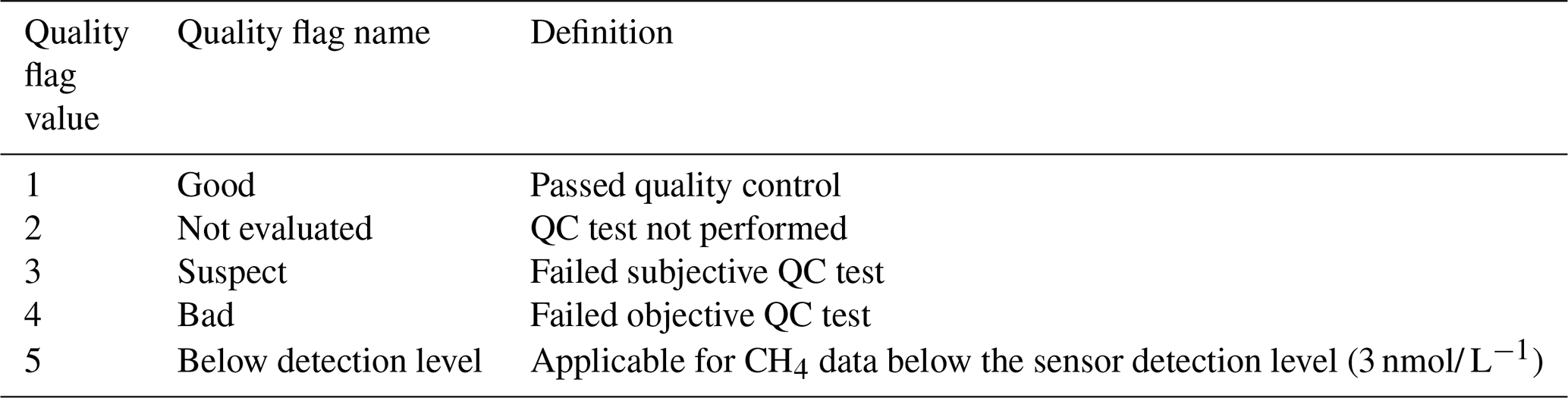
Based on UNESCO's best oceanographic practices (https://repository.oceanbestpractices.org/handle/11329/413, last access: 15 February 2024), which are also used for Argo floats, an objective and automatic quality control (QC) process was applied. Quality flags (QFs) are composed of four quality values (Table 2).

Table 2 Quality flag scheme.

The procedure allows us to flag outliers but may be deficient in identifying some erroneous data. Tests presented hereafter relate to the other variables and are based on published methods (Pouliquen et al., 2010; Schmechtig and Thierry, 2016) and are recommended by the scientific community through international programmes, such as the EGO quality control manual for CTD and BGC (BioGeoChemical) data (https://archimer.ifremer.fr/doc/00403/51485/92689.pdf, last access: 4 August 2024).

A gross filter is applied on observed data using a global range test first (Table 3), with min and max values taken from World Ocean Atlas 2018 documentation (Garcia et al., 2019).

Table 3 Global range test derived from World Ocean Atlas 2018 climatology used for QC.

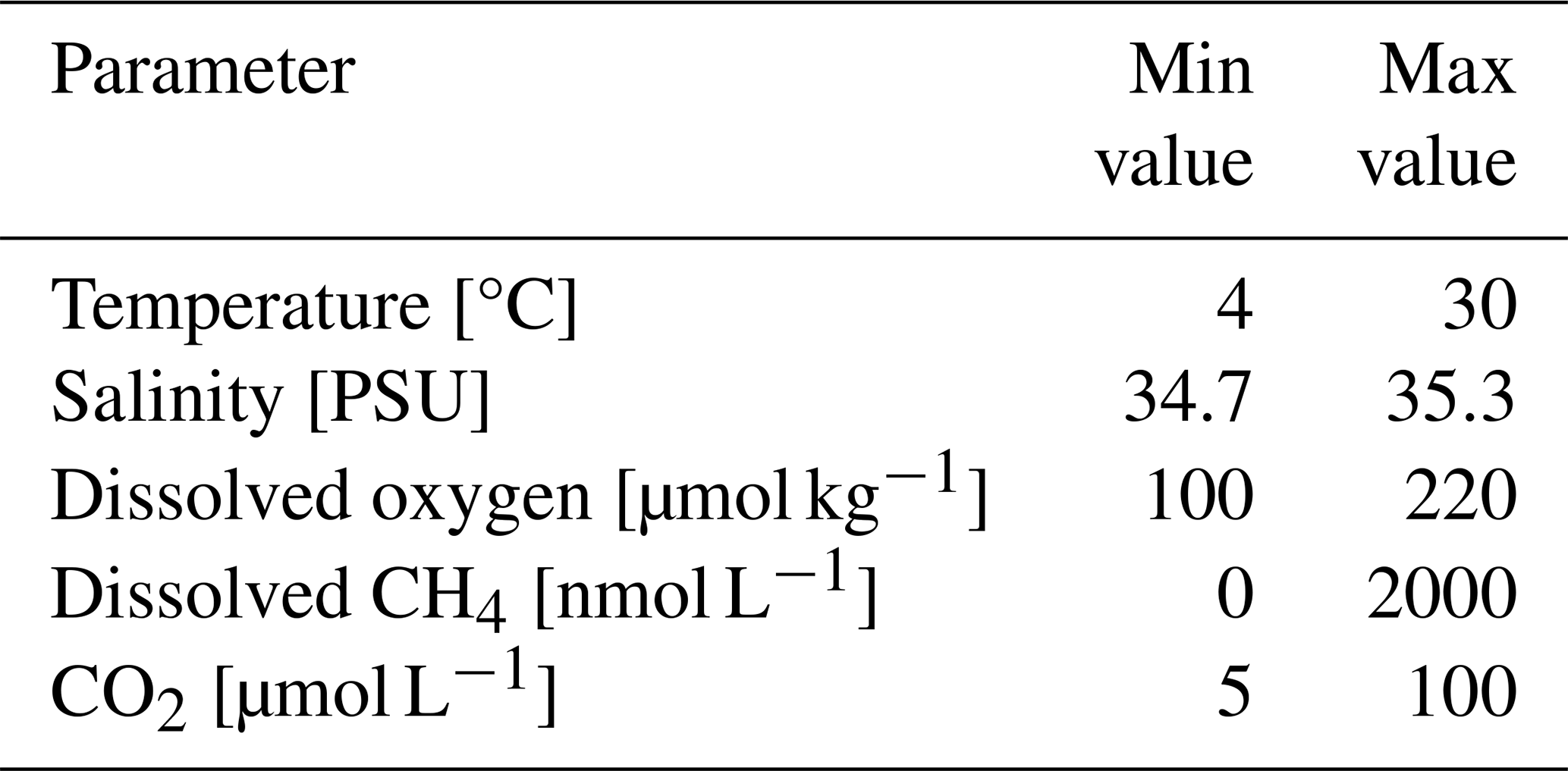
Values that fail this test are flagged with a QF of 4. To our knowledge there is not yet an international recommendation for CH₄ and CO₂; thus, values were chosen based on in situ measurements from MAYOBS cruises.

For all parameters, data acquired when the CTD pressure is negative (i.e. in-air measurement) were flagged as bad (QF of 4).

Furthermore, a large difference between sequential measurements, where one measurement greatly differs from adjacent ones, was also flagged bad if failing the following algorithm (only used to identify spikes in temperature, salinity and O₂ profiles; EGO quality control manual, 2022):

$$\begin{array}{}\text{(5)}& \mathrm{Test}=\mathrm{|}{\displaystyle \frac{\mathrm{V}\mathrm{2}-(\mathrm{V}\mathrm{3}+\mathrm{V}\mathrm{1})}{\mathrm{2}}}\mathrm{|}-\mathrm{|}{\displaystyle \frac{\mathrm{V}\mathrm{3}-\mathrm{V}\mathrm{1}}{\mathrm{2}}}\mathrm{|},\end{array}$$

where V2 is the measurement being tested as a spike, and V1 and V3 are the values preceding and ensuing. The V2 value is flagged when the test value exceeds the following:

• TEMP – 6.0 °C for PRES < 500 db or 2.0 °C for PRES ≥ 500 db

• SAL – 0.9 for PRES < 500 db or 0.3 for PRES ≥ 500 db

• O₂ – 50 µmol kg⁻¹ for PRES < 500 db or 25 µmol kg⁻¹ for PRES ≥ 500 db.

To our knowledge there are, to date, no international recommendations for CH₄ and CO₂. Thus, no spike test was applied to these variables. Finally, subjective visual inspection was performed for each variable to identify outliers that were not flagged by the automatic and objective procedure. These measurements were associated with a QF of 3.

Membrane-based sensors (CO₂ and CH₄) are also deficient at high glider speeds (lag cannot be compensated for correctly). Thus, CO₂ and CH₄ data acquired at glider speeds exceeding 0.25 m s⁻¹ were flagged and excluded. This usually occurred when the glider rarely ascended in an alarm state.

All data provided have been quality controlled. Therefore, a QF of 2 is not used in this data set.

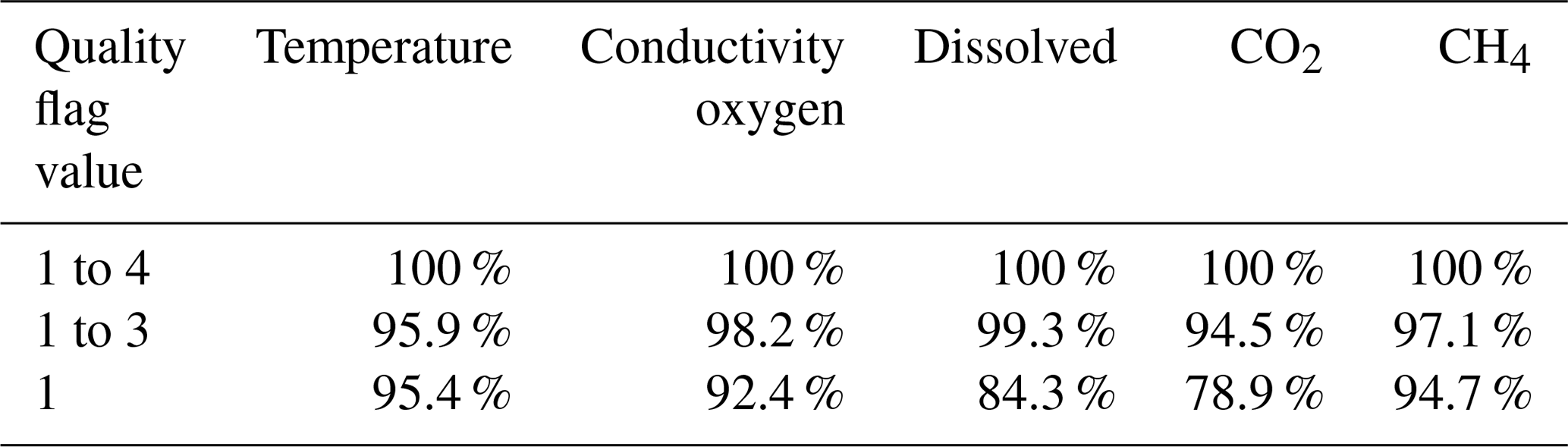
Following these various objective and subjective tests, the remaining data volume of each data set is provided in Table E1.

Every 6 months, a reassessment of the processing chain (algorithm, QC) and delayed-mode adjustments (drift, offset) is proposed.

3 Results and discussion

3.1 Hydrological data set

Hydrological data presented are adjusted and associated with a QF of 1.

Time series of temperature, salinity and potential density are presented in Fig. 3; averaged vertical profiles are presented in Fig. 4; and a temperature–salinity diagram exhibiting the different water masses is shown in Fig. 5.

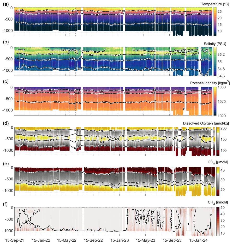
Figure 3 Temperature (a), salinity (b), potential density with a reference pressure of 0 dbar (c), dissolved oxygen (d), CO₂ (e) and CH₄ (f) Hovmöller diagram as a function of depth (y axis) and time (x axis). Isolines are calculated by applying a Gaussian filter of size 7 to each data field. White areas correspond to time periods with no data due to sensor downtime or glider recovery.

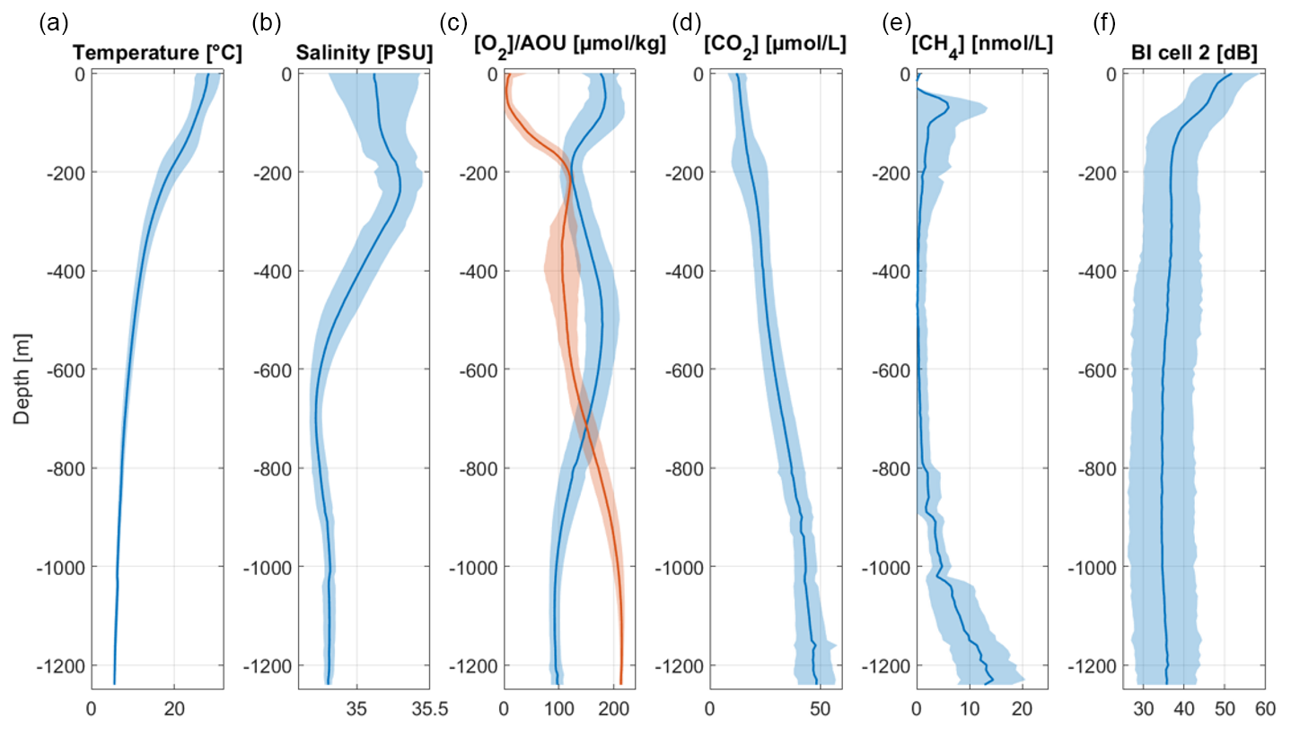
Figure 4 Averaged vertical profiles of temperature (a), salinity (b), O₂ (blue) and apparent oxygen utilization (AOU, orange) (c), CO₂ (d), CH₄ (e), and backscatter index (BI) calculated from cell 2 of the ADCP (f) over 10 m bins for the whole data set, with variability represented as ±2 standard deviations (shaded areas).

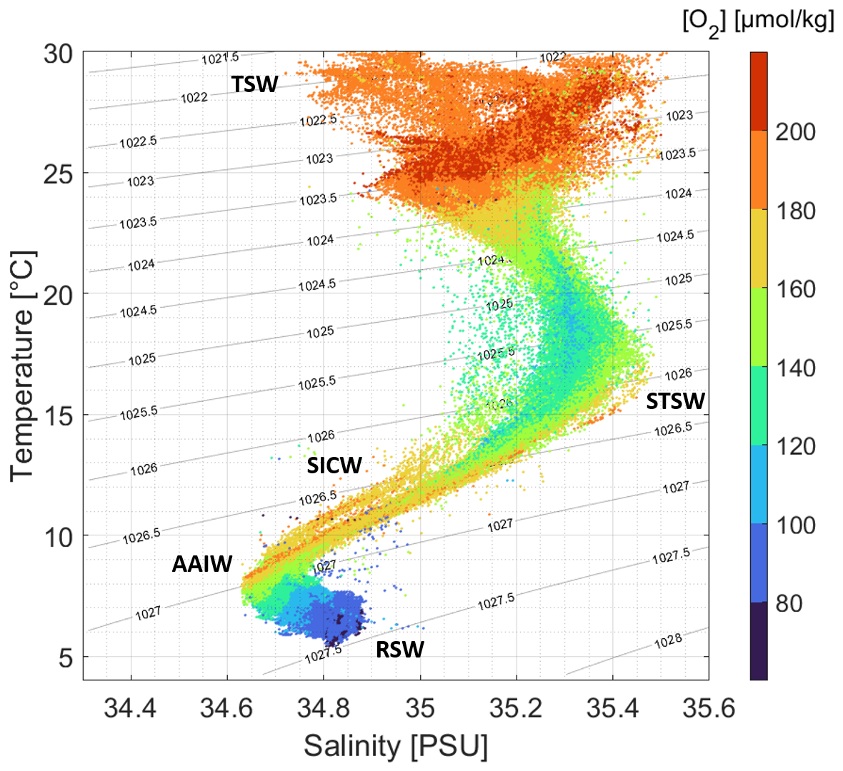
Figure 5 Temperature–salinity diagram. The colour indicates the O₂ concentration, and the associated water masses are annotated. TSW stands for tropical surface water, STSW stands for subtropical surface water, SICW stands for South Indian Central Water, AAIW stands for Antarctic Intermediate Water, and RSW stands for Red Sea Water.

As for temperature, vertical profiles exhibit a relatively warm upper layer (∼0–100 m, 26–30 °C). The seasonal thermocline (steep thermal gradient of ∼0.1 °C m⁻¹) is observed between ∼100–200 m, and the permanent thermocline is located at ∼500 m and is mainly composed of South Indian Central Water (SICW, Miramontes et al., 2019).

Below 500 m, temperatures are in the range of 5–10 °C, with a minimum reached below 1000 m. In this layer, both Red Sea Water (RSW), which enters into the Mozambique Channel from the north, and Antarctic Intermediate Water (AAIW), which enters from the south, are found (Miramontes et al., 2019).

The vertical distribution of the salinity is more complex. Overall, the upper layer is characterized by values starting from ∼34.7 and 35.5 PSU. A subsurface salinity maximum is observed at ∼200–300 m, with salinity values reaching up to 35.5 PSU. At around 600 m, a local salinity minimum (34.6–34.8 PSU) is observed but is followed by a slight increase to reach ∼34.85 below 1000 m.

Deeper in the water column (i.e. below ∼100 m), the variability in hydrological properties is lower. However, disruptions in the vertical distribution of temperature and salinity are visible, such as between June and July 2022 (between the dotted grey lines in Fig. 3) and can be attributed to the general circulation of the area or the mesoscale variability. Below 1000 m, the variations are ∼1 °C and ∼0.1 for temperature and salinity, respectively (Fig. 6).

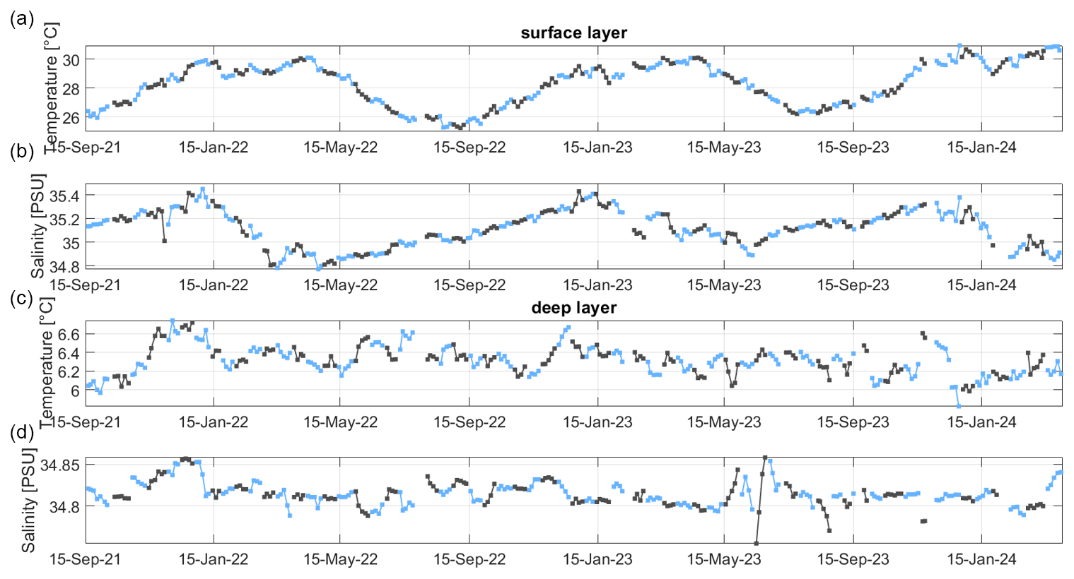
Figure 6 Surface layer (0 to 5 m) daily average temperature (a) and salinity (b) and deep-layer (950 to 1250 m) daily average temperature (c) and salinity (d). Colour alternation reflects the succession of glider missions.

Most of the temporal variability is observed in the surface layer, above the 1024 kg m⁻³ isopycnal. These changes are particularly obvious in the temperature–salinity diagram (Fig. 5) indicating the succession of two distinct water masses (Collins et al., 2016). Indeed, low salinity values are typical of the tropical surface water and contrast with the higher-salinity subtropical surface waters (Di Marco et al., 2002). Surface temperatures exceeding 29 °C (which are regularly observed from December to April, Figs. 4 and 7) can also be the signature of the influence on the South Equatorial Current that contains Pacific waters (Di Marco et al., 2002) or associated with the transient presence of mesoscale eddies. Finally, in accordance with Wyrtki (1971), seasonal processes (and episodically tropical storms) may also account for the observed variability. The highest sea surface temperatures and low salinities are generally observed during austral summer, while, in winter, colder and saltier waters dominate. This seasonal variability is observed in this part of the water column (Fig. 7), with warm (∼27–28 °C) and salty (∼35.3–35.4) surface waters from November 2021 to July 2022 and from October 2022 to July 2023 during the warm and humid austral summer in Mayotte.

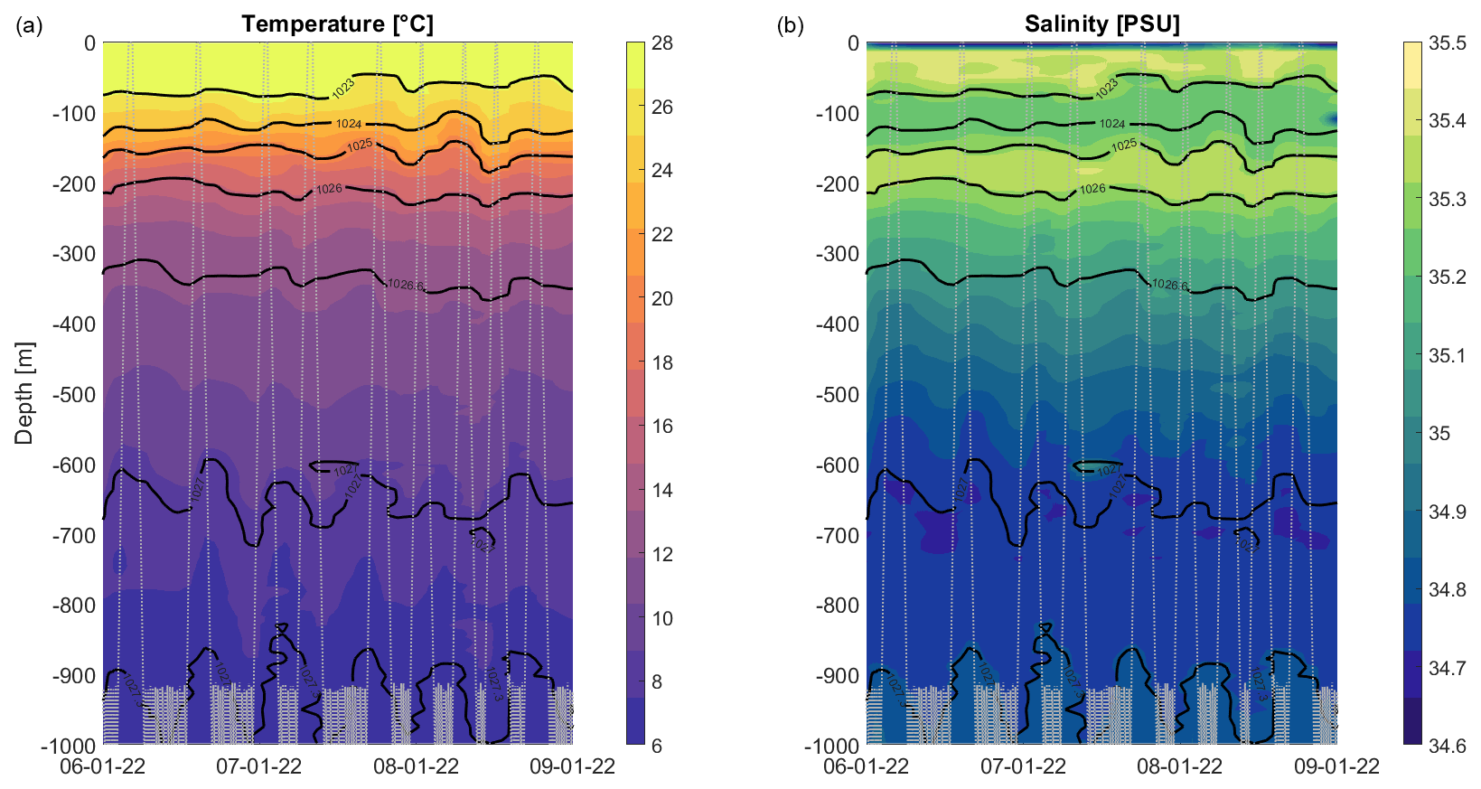
Figure 7 High-frequency (∼12 h period) oscillations of temperature (a) and salinity (b) as a function of depth (y axis) and time (x axis). Glider depth is represented by the dotted light-grey line, and isopycnals are also calculated and displayed in black. Data are interpolated with a triangulation-based cubic interpolation over a 12 m grid.

The analysis of the data set also highlighted the importance of smaller-temporal-scale processes, particularly vertical fluctuations of potential density levels (and temperature and salinity) per hour (Fig. 7). Likely a result of internal tides, the sampling strategy chosen, consisting of deep multi-yo patterns, unfortunately does not allow their quantification (Sect. 2.2.4).

3.2 Dissolved gas data set

Similarly to the hydrological data set, data presented are adjusted and associated with a QF of 1.

Measured O₂, CO₂ and CH₄ concentrations by the glider are shown in Fig. 3. Typical vertical distributions are observed (Fig. 4) and can be explained by ubiquitous physical (e.g. dissolution, sea–air exchanges) and biological oceanic processes (photosynthesis and respiration).

High O₂ concentrations corresponding to oxygen saturation concentration are measured (O₂ concentrations of about 180–200 µmol kg⁻¹, apparent oxygen utilization between 0–20 µmol kg⁻¹, Figs. 3 and 4) at the surface layer (0–100 m) because of both dissolution from the atmosphere and O₂ production by phytoplankton. The study area, located off the coast of Mayotte, is generally characterized by oligotrophic conditions, typical of tropical oceanic regions (Ternon et al., 2014). Such conditions are associated with low concentrations of nutrients in surface waters, which constrain primary production and consequently limit biological oxygen supersaturation. Nevertheless, the presence of detectable surface O₂ saturation suggests that, despite low nutrient availability, the prevailing light conditions and water column stratification support moderate phytoplankton activity in the upper layer. As the distance to the surface increases O₂ generally declines due to O₂ removal by consumption of deep-water organisms and by the decomposition of organic material by bacteria (Hedgpeth, 1957). In the glider data set, minimum O₂ values (O₂ in the range of 70–100 µmol kg⁻¹) are observed below 1000 m. In spite of this decrease, O₂ contents rise to a subsurface maximum at ∼400–500 m, with values reaching up to 200 µmol kg⁻¹. This high O₂ core (>180 µmol kg⁻¹) is characteristic of the South Indian Central Water (Di Marco et al., 2002).

Regarding the CO₂ vertical distribution (Fig. 4), it is essentially the reverse of O₂, mainly because both gases are involved in the same biological processes in opposite ways. At the surface, photosynthesis consumes CO₂, and, thus, concentrations are low (∼15 µmol L⁻¹). In deeper waters, CO₂ concentration increases as respiration exceeds photosynthesis, and decomposition of organic matter adds additional CO₂ to the water. In this data set, minimum CO₂ concentrations are found in the surface layer (0 - 100 m), with concentrations measured to be between 15–20 µmol L⁻¹, and maximum CO₂ values are measured below 1,000 m depth, with concentrations generally higher than 40 µmol L⁻¹ and sporadically exceeding 50 µmol L⁻¹. Moreover, the signature of SICW, with its oxygen maximum at ∼400–500 m (Di Marco et al., 2002), is not matched by a CO₂ minimum at this depth.

The vertical distribution of CH₄ differs significantly from the ones of O₂ and CO₂ (Figs. 3 and 4). Almost no CH₄ is detected in the 0–600 m layer (values are below 10 nmol L⁻¹). This is not surprising because the ocean is supposed to be depleted in CH₄, save for specific areas (methanogenesis in marine sediments, natural seepage by volcanoes or hydrothermal vents, pollution; Oremland and Taylor, 1978). Most CH₄ increases occur in the 900–1250 m layer, where the sampling effort is at its maximum. In this layer, when CH₄ anomalies are detected (above the sensor detection limit), a gradient of increasing concentration with depth is observed. High values relative to the background are regularly observed, with a maximum recorded on 18 February 2022, when CH₄ reached 120 nmol L⁻¹ at a 1000 m depth. Although observations above 900 m are scarcer than below, several vertical profiles also show significant CH₄ concentrations up to 700 m.

There is also variability in dissolved gas concentrations, with periods (e.g. September 2022 to mid-October 2022 and mid-November 2022 to February 2023) of decreasing CH₄ or CO₂ concentrations that are not yet explained (Fig. 8).

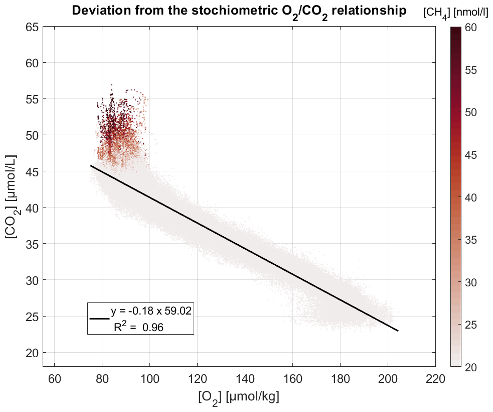
Figure 8 O₂–CO₂ relationship below 700 m; the colour bar indicates the CH₄ concentration. Data are taken from September 2021 to January 2023 and below 600 m.

Considering the amount of data produced, semi-automatic methods are thus required to reduce this data set to relevant information. Here we focus on parameters that track magmatic fluid emissions (CO₂ and CH₄) and define anomalies as observations that deviate significantly from the majority of the data.

Identifying anomalies (that refer to fluid emissions) is challenging since it requires decoupling between natural variability (e.g. water masses, seasonality) and changes induced by fluid emissions. In particular, CO₂ and CH₄ signals are characterized by slowly varying background values related to dissolved gas accumulation and flushing over a large area. The CH₄ baseline is low (<10 nmol L⁻¹) and has a magnitude of variability of about 6 nmol L⁻¹. On the other hand, the CO₂ baseline is more elevated (∼45 µmol L⁻¹ at a 1250 m) because of the natural presence of CO₂ in seawater and CO₂ anomalies below 900 m, but fluctuations around the mean values do not exceed ∼3 µmol L⁻¹.

Results also show that both CO₂ and CH₄ baselines have similar temporal evolutions, supporting the hypothesis that this variability is likely to be real. For the purpose of anomaly detection, the baseline was thus subtracted from the raw data:

$$\begin{array}{}\text{(6)}& \begin{array}{rl}\mathrm{Gas},{\mathrm{anomaly}}_{\mathrm{deep}}\left(t\right)& =\mathrm{Gas},{\mathrm{measured}}_{\mathrm{deep}}\left(t\right)\\ & -\mathrm{Gas},{\mathrm{baseline}}_{\mathrm{deep}}\left(t\right).\end{array}\end{array}$$

However, the cause of this low-frequency variability still remains to be clarified. At this time, it is not clear if baseline fluctuations are related to accumulation–dispersion processes or induced by changes in fluid emission rates, both compatible with the chosen anomaly definition.

Of the 22 000 profiles, 5 % were associated with significant CH₄ anomalies (greater than the sensor detection limit plus twice the standard deviation), and 2 % were associated with significant CO₂ anomalies related to dissolved gas emissions (same definition as for the CH₄).

Data show that CO₂ and O₂ have similar patterns. Such a co-variation is expected in the ocean and is related to biotic processes. Examining this relation at a depth > 700 m (i.e. below the STSW) indeed confirms a high CO₂ and O₂ correlation (linear correlation coefficient, R²=0.96). Several single measuring points deviate from the linear relationship (Fig. 8). They are all found in the upper curve, i.e. at a depth where CO₂ is high and O₂ low. Most of these points are also independently associated with high CH₄ concentrations, which strongly suggests that these CO₂ anomalies are related to a non-biotic CO₂ source.

3.3 Ocean current and acoustic backscatter data set

ADCP-derived water currents show a large profile-to-profile variability that encompasses, in all likelihood, spatial and temporal variability. The strongest currents are measured in the surface (0–100 m layer), but velocities remain elevated down to 1250 m (Fig. 9).

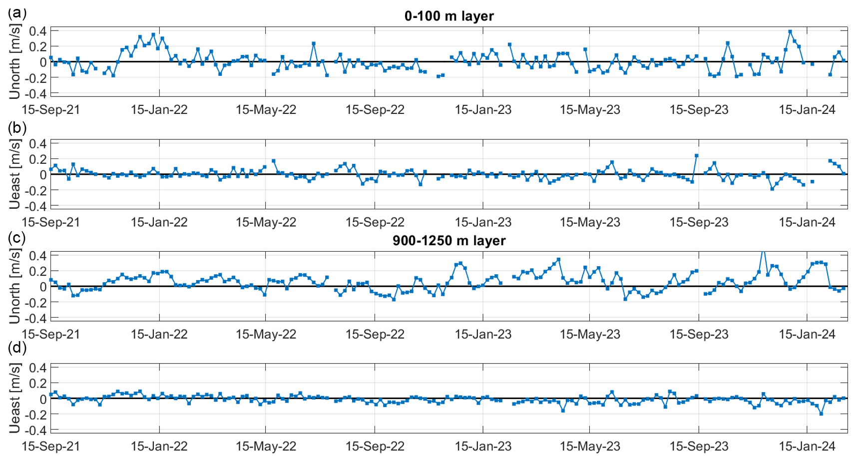
Figure 9 Time series of northward (a) and eastward (b) velocities measured by the ADCP in the 0–100 m layer and time series of northward (c) and eastward (d) velocities measured by the ADCP in the 900–1250 m layer. The data shown correspond to daily mean values, computed separately for the depth layers: the surface layer (0–100 m) and the deep layer (900–1250 m).

Overall, eastward velocities do not exhibit clear patterns. Values oscillate with no preferential direction (Fig. 9). Conversely, northward velocities are characterized by a distinguishable temporal variability. From several weeks to several months, the current direction changes, with long periods of time when the direction of flow remains unchanged. The strongest currents appear to be aligned with the continental slope (north–south axis), which may be related to barotropic currents.

Strong deep currents (≈0.4–0.5 m s⁻¹) below 900 m are also present in the area and are locally highly variable, with strong interactions with the bathymetry and the tide (Fig. 9).

Backscatter data estimated from ADCP measurements and expressed as the backscatter index (BI) are represented in Fig. 4 as an averaged profile. This averaged profile primarily depicts water mass optical property changes which are determined by phytoplankton and zooplankton abundance and mineral particle concentrations (Mullison, 2017; Gentil et al., 2020). Thus, as can be expected, the BI shows maximum values in the surface layer (0–100 m), where most of the biological activity takes place. Deeper in the water column, the BI is generally lower, although sometimes peaking at the level of the South Indian Central Water and in the ∼900–1250 m layer when crossing dissolved gas plumes or moving around the seafloor.

Similarly, the BI variability in the surface mirrors changes in temperature and salinity to a certain extent, and several glider dives showed a BI increase at depth, when the glider approaches the continental shelf. This variability is not fully understood and is likely to have a multi-factor cause resulting from a decoupling of the surface, subsurface and deep dynamics. Whatever the processes envisioned, in all likelihood, a direct contribution of magmatic fluid emissions can be discarded.

On the other hand, BI profiles are noisy and variable with depth, and, despite this large variability, the signature of bubbles and/or droplets appears to be unambiguous, associated with a large density of positive spikes of great amplitude and associated vertical velocity anomalies of about 15 cm s⁻¹, which is the ascent velocity of millimetre-sized gas droplets in seawater (Rehder et al., 2009; Leblond et al., 2014, Fig. 10). The BI increases in the deep layer were considered to be related to bubble and/or droplet plumes if several consecutive BI values exceeded ∼50 dB in at least six cells of the ADCP in order to discard the few possible misdetections at this depth. This was used as a criterion for BI anomaly detection, but each dive was also visually inspected.

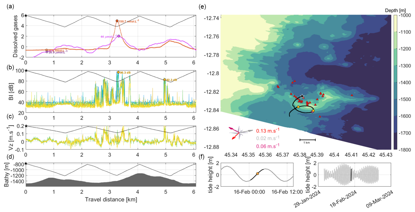
Figure 10 Example of a glider between the 800–1250 spiral track carried out above known fluid active sites. (a–d) CO₂ and CH₄ concentrations are represented, respectively, in red and purple, centred and reduced (to get a common representation of the two dissolved gases despite the different baselines and anomalies) as a function of the dive progress (a). The minimum and maximum of each data are represented by a circle. BI data calculated from each paired cell of the ADCP (b), followed by vertical velocity calculated from the ADCP data (c) and, finally, the bathymetric profile throughout this dive (d). Isobath map of the Horseshoe area, with the underwater glider position in black, including the plot of direction and velocity for different currents calculated during this dive (surface geostrophic current in red, ADCP-calculated 800–1250 m deep current in purple and tidal current in grey) (e) and the local tide height (f). Surface geostrophic current is estimated from sea level anomaly (SLA) data computed with respect to a 20-year ([1993, 2012]) mean (https://doi.org/10.48670/moi-00149, E.U. Copernicus Marine Service Information, Marine Data Store, 2024). Tidal current parameters are computed with the MIKE21 model.

Of the 22 000 profiles, 457 (∼2 %) were associated with significant BI anomalies. The relatively low occurrence of BI detections indicates that bubble and/or droplet plumes are likely to be of limited spatial extension (∼ hundreds of metres) especially compared with dissolved and neutrally buoyant gas plumes.

Although associating BI detections directly with a fluid emission active site is complex (uncertainty in glider positioning, tilt of droplets and/or bubbles plumes of several hundred metres because of deep and tidal currents), data show that most of the known active sites were indeed identified by the glider; 95 % of BI detections are found within a radius of 700 m from an active site, and the remaining 5 % are always found at a distance of less than 1.6 km.

Repeated dissolved gases and BI anomalies in the 800–1250 m layer (Fig. 10) provide evidence that elevated CO₂ anomalies in the 900–1250 m layer are related to magmatic fluid emissions from the seafloor.

BI detections outside of the 95th percentile observed around the Horseshoe zone may arise from intermittent, small, unidentified sites or false detections. Further analysis is needed to confirm the nature of these detections.

Temporal variations in dissolved gas concentrations (CH₄ and CO₂) and BI anomalies are presumably caused by a complex array of factors, including spatial variability related to the glider pathway. However, on the basis of our current knowledge, we assume that a large part of the observed changes can indeed be related to the variability of seafloor fluid emissions in the Horseshoe area, as well as the orientation and direction of the current at depth.

3.4 Discussion

Over the 30 months of deployments, values of CH₄ and CO₂ show some interesting patterns, with a large profile-to-profile variability observed in dissolved gas deep anomalies. High anomaly values exceeding the detection limit of the sensor plus 2 times the standard deviation (20 $nmol/l$ for the CH₄ anomalies and 7 µmol L⁻¹ for the CO₂ anomalies) are observed throughout the time series. In the 900–1000 m layer (more than 90 % of the data set), the maximum CH₄ anomaly value is reached on 21 February 2022 (116.9 nmol L⁻¹), and the maximum CO₂ anomaly value is reached on 4 September 2022 (29.2 µmol L⁻¹).

Although a direct correlation between currents and gas anomalies is speculative, our data suggest a potential impact of mesoscale structures on gas concentrations in the 900–1250 m layer. The underlying processes are still poorly understood from the sole analysis of the glider data set, but several processes would be worth investigating (e.g. trapping of gas bubbles in stratified layers, lateral dispersion by mesoscale flows, vertical diffusion of dissolved gases, or upwelling induced by topographic features or internal waves). Furthermore, additional bottom current data could potentially be useful for this analysis. In order to assess the spatial distribution, anomalies are plotted on maps (Fig. 11). This provides a comprehensive view of the area impacted by fluid emissions over the 30-month duration of deployments. In Fig. 11, data are binned in seven discrete concentration intervals and superimposed from weakest to strongest with circles of decreasing size. Only data that exceed the criteria of detection are coloured, and the maxima of the colour bar are equal to the 99th percentile.

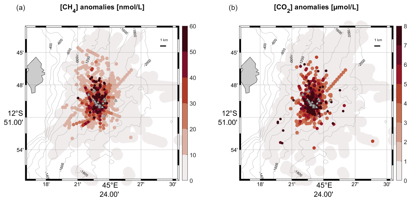
Figure 11 Map of CH₄ (a) and CO₂ (b) anomalies above the detection limit of these sensors recorded during the whole glider survey. The grey triangles are the active fluid emission sites identified with the multibeam echo sounder during the REVOSIMA MAYOBS cruises (https://doi.org/10.12770/070818f6-6520-49e4-bafd-9d4d0609bf7d, Scalabrin, 2023) and validated by in situ visual observations with the ROV VICTOR during the GEOFLAMME cruise (https://doi.org/10.17600/18001297, IFREMER, 2021).

The highest gas anomalies were all observed in the centre and in the immediate vicinity of the Horseshoe edifice, and the magnitude of the anomalies progressively decreased as the glider moved away from the centre. The radius of gas anomaly detection is around 10 km, and the total area impacted by fluid emissions spread over about 300 km². These maps, which gather all data from 17 September 2021 onwards, also show that the distributions of gas anomalies are not isotropic. In particular, relatively high concentrations relative to the far field are observed northward, which can highlight a preferred export direction for these quantities of dissolved gas.

Many questions still remain with regard to our understanding of the underlying processes. We can, for example, mention the spatial decoupling between acoustic and dissolved gas plumes or the contribution of physical factors in modulating the extension, direction and intensity of the plumes (currents, internal tides).

To deal with these scientific challenges, the synergy between the glider with other observation and measurement tools (CTD casts, remotely operated vehicles (ROVs), moorings), numerical models, and satellite products is promising. Several studies in this direction have been initiated, and although clear results are not yet available, ongoing work is progressing steadily.

Reference data acquired during MAYOBS cruises allowed for a cross-calibration exercise of the dissolved gas sensors. An exercise was carried out during the MAYOBS25 cruise in September 2023 and during the MAYOBS30 cruise in September 2024 by harnessing two gliders on the CTD cast in order to compare dissolved gases from glider sensors and Niskin samples. The aim of these calibrations is to quantitatively calibrate dissolved gas sensors in order to calculate the fluxes of fluids emitted at the seabed. The database will be updated accordingly for the time period covered by this study once the CH₄ and CO₂ sensor calibrations are finalized. Additional data sets will also be made available in the future as the mission is ongoing. Since the project is funded by the French government, all validated data will be made publicly accessible.

4 Data availability

Raw and processed data are available from the SEANOE data centre: https://doi.org/10.17882/99960 (Heumann et al., 2024).

5 Conclusions

The data set presented here demonstrates the feasibility of collecting long-term physico-chemical measurements (including CTD; ADCP; and dissolved gases such as O₂, CH₄ and CO₂) using a glider platform over periods extending up to 30 months, with interruptions limited to deployment and/or recovery operations and brief maintenance interventions.

This is one of the few glider missions that has simultaneously sampled CH₄ and CO₂ data, as well as being the longest glider time series of these dissolved gas measurements that we are aware of. It also opens the possibility for new projects and research with the ability to detect and monitor CH₄ and CO₂ underwater distributions (e.g. GEORGE project (Next Generation Multiplatform Ocean Observing Technologies for Research Infrastructures, https://george-project.eu/, last access: 2 February 2025), Hauri et al., 2024).

The vertical distribution of hydrological, dissolved gas and BI data highlighted anomalies due to magmatic fluids in the Horseshoe area, while ADCP-calculated current depicted an active area subject to strong currents both at the surface and at depth.

The data analysis is still ongoing, but the glider platform showed its ability to monitor, track and characterize seafloor fluid emissions mainly composed of CO₂ droplets off Mayotte Island. This experiment proves the feasibility of integrating a glider into a real-time early-warning system. In particular, the continuous monitoring at a high spatio-temporal scale of the 0–1250 m layer appears to be relevant to complement traditional oceanographic cruises (synoptic and high-quality data but with a limited temporal scale) and to ensure an operational observing system.

The robustness of the platform (SeaExplorer glider) has also been demonstrated thanks to this data set, with 901 d at sea over 929 d (97 % of its time spent at sea).

The quasi-permanence of elevated gas concentrations (CO₂ and CH₄) in the Horseshoe area supports the fact that fluid emissions are likely to have been continuous and detectable over the 30 months of the mission.

Regular detections of acoustic plumes above all identified active sites have provided direct evidence of active seepage during the survey and the presence of bubbles and/or droplets above 1250 m depth.

Appendix A

Table A1 Glider missions performed with deployment and recovery, glider used, mission ID, and sensor serial numbers.

Appendix B

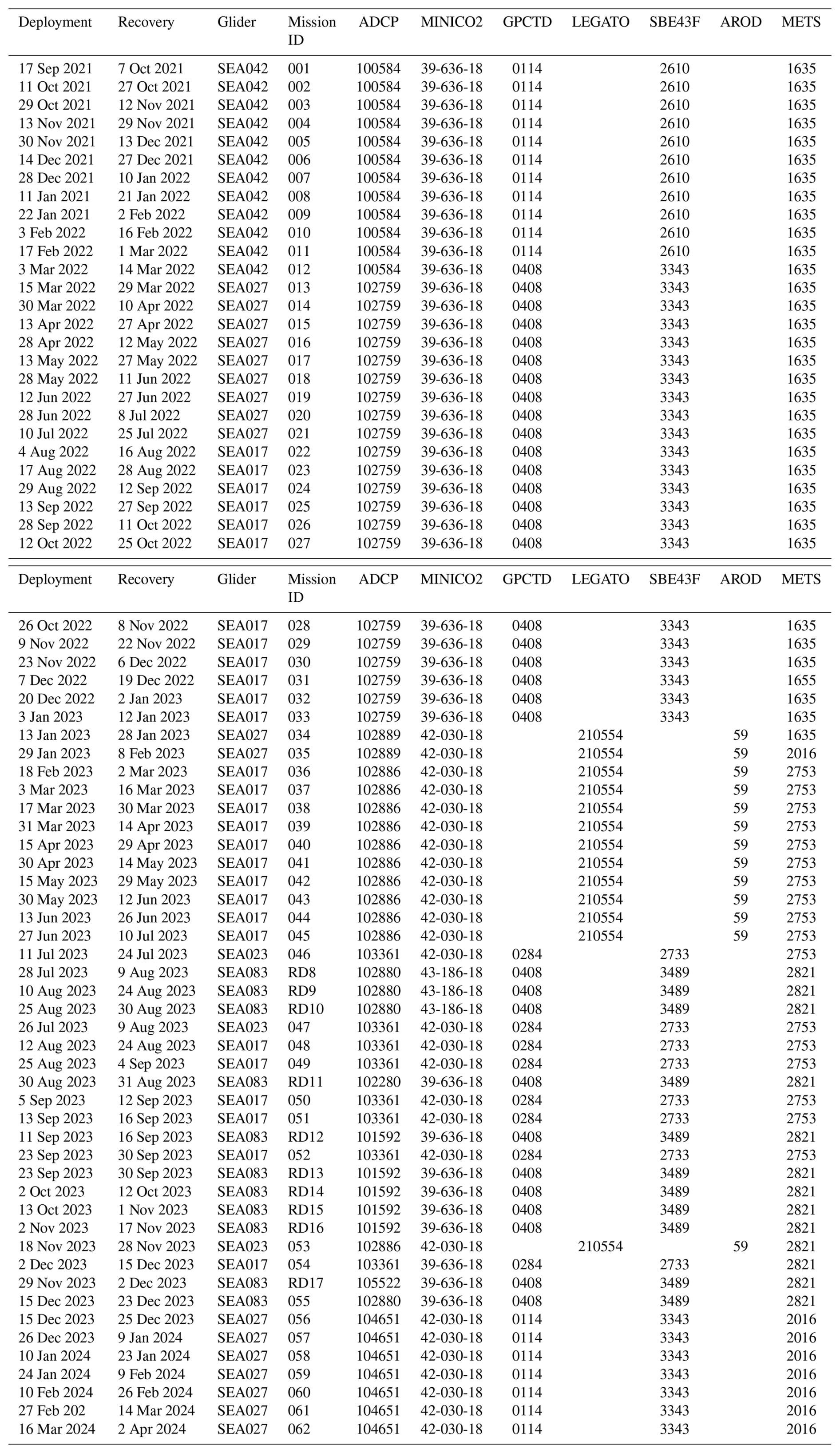
Table B1 Gain values applied to O₂ data depending on the dive number, with reference profiles acquired during MAYOBS cruises.

Appendix C

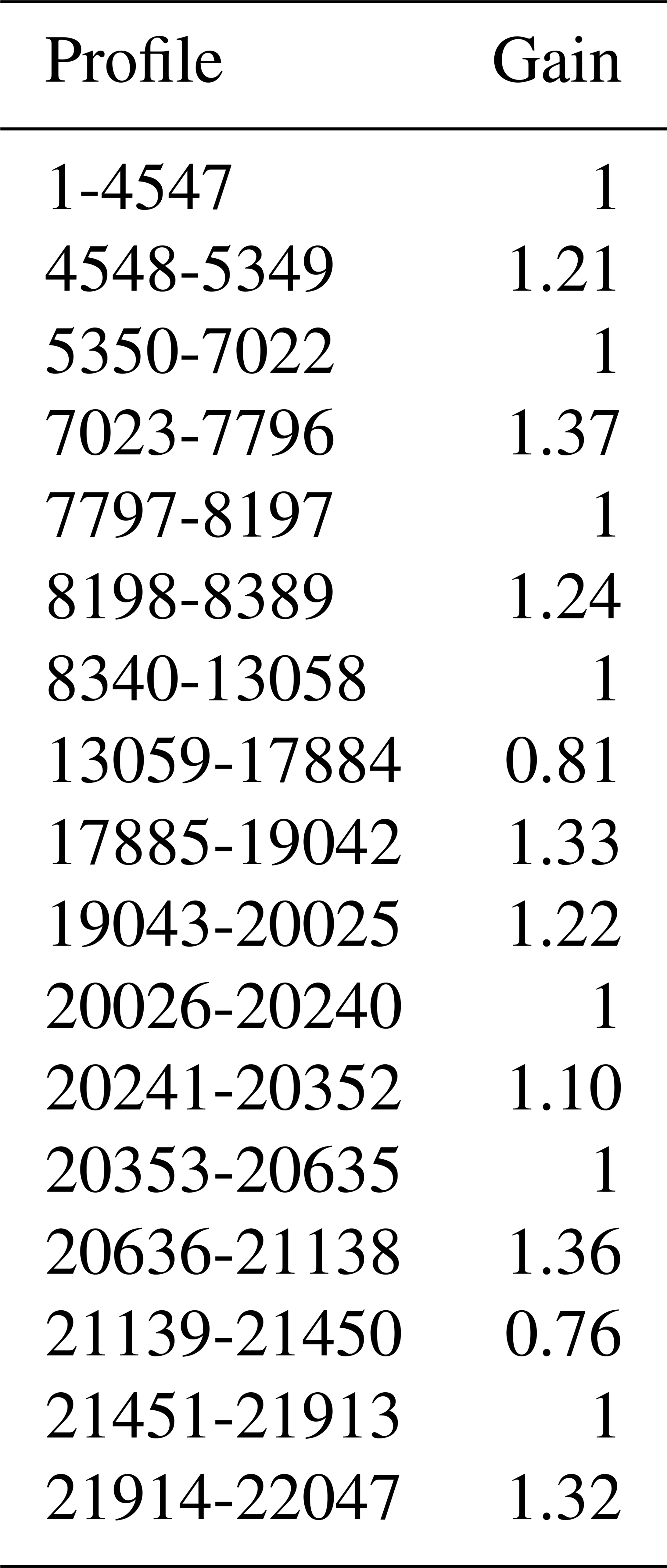
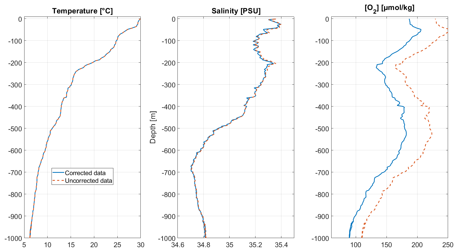
Figure C1 Vertical profiles of corrected (blue) and uncorrected (red) temperature, salinity and O₂ concentration as a function of depth from dive no. 13089.

Appendix D

Table D1 Sensor information.

Appendix E

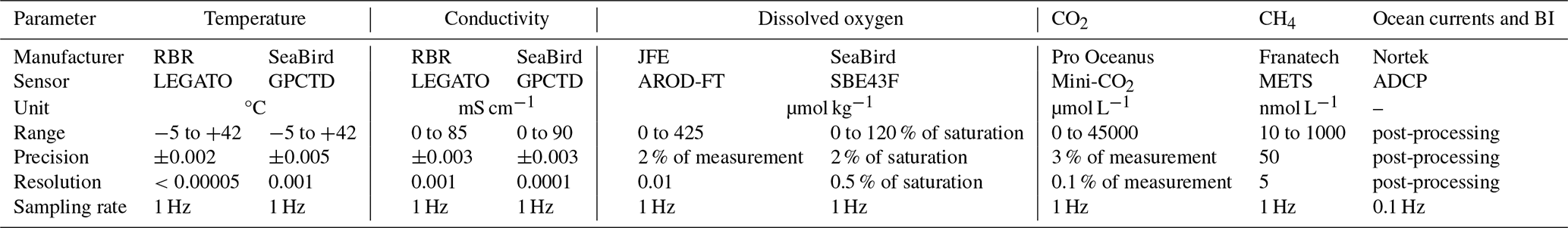
Table E1 Percentage of total data going through QC (total number of points for each data set is 2 232 706).