Satellite-based analysis of ocean-surface stress across the ice-free and ice-covered polar oceans

Ocean-surface stress is a critical driver of polar sea-ice dynamics, air–sea interactions, and ocean circulation. This work provides a daily analysis of ocean-surface stress on 25 km Equal-Area Scalable Earth (EASE) grids across the ice-free and ice-covered regions of the polar oceans (2011–2021 for the Arctic, 2013–2021 for the Antarctic), covering latitudes north of 60° N in the Arctic and south of 50° S in the Antarctic and Southern Ocean. Ocean-surface stress is calculated using a bulk parameterization approach that combines ocean-surface winds, ice motion vectors, and sea surface height (SSH) data from multiple satellite platforms. The analysis captures significant spatial and temporal variability in ocean-surface wind stress and the resultant wind-driven Ekman transport, while providing enhanced spatiotemporal resolution. Two sensitivity analyses are conducted to address key sources of uncertainty. The first addresses the fine-scale variability in SSH fields, which was mitigated using a 150 km Gaussian filter to smooth 3 d SSH datasets and enhance compatibility with the other monthly product, followed by linear interpolation to achieve daily resolution. The second investigates uncertainty in the ice–water drag coefficient, which revealed that variations in the coefficient have a proportional influence on the computed ocean-surface stress under the tested conditions. These uncertainties are most pronounced during winter, with median values reaching 20 % in the Arctic and 40 % in the Southern Ocean. Validation efforts using ice-tethered profiler velocity records revealed weak to moderate correlations with satellite-derived stress (r= 0.4–0.8) between observed surface velocities and satellite-derived estimates (Ekman + geostrophic) at daily resolution, with significantly improved agreement when averaged to weekly means. This dataset is publicly available at https://doi.org/10.5281/zenodo.15534576 (Liu and Yu, 2024).

1 Introduction

Earth's polar regions have undergone profound changes over the past decades, with sea ice playing a central role in the polar climate system. By modulating heat, momentum, and freshwater exchanges at the atmosphere–ice–ocean boundary, sea ice directly influences global climate dynamics (Meehl, 1984; Stammerjohn et al., 2012). In the Arctic, rapid sea-ice decline has transitioned the region from predominantly thick, multiyear ice to thinner, more dynamic ice, with increased interannual variability (Comiso et al., 2008; Stroeve and Notz, 2018; Moore et al., 2022; Babb et al., 2022). Meanwhile, Antarctic sea-ice trends have shown greater complexity, with a modest long-term increase observed until the mid-2010s, followed by a record loss in 2017 and a subsequent continued decline (Liu et al., 2004; Parkinson, 2019; Turner et al., 2022; Purich and Doddridge, 2023). These changes in sea-ice extent and thickness have significant implications for polar systems and global climate feedbacks, influencing the Arctic's ability to regulate planetary heat, as well as impacting marine ecosystem, carbon cycling, nutrient distribution, and thermohaline circulation (Talley, 2013; Campbell et al., 2019).

Atmospheric circulation is a primary driver of sea-ice dynamics and variability. Geostrophic winds, for instance, account for over 70 % of sea-ice velocity variability (Thorndike and Colony, 1982; Maeda et al., 2020), while broader climate modes, including the Arctic Oscillation, Pacific Decadal Oscillation, and Southern Annular Mode, influence ice extent and distribution (Rigor et al., 2002; Park et al., 2018; Lefebvre et al., 2004). These wind-driven processes interact with sea ice to modify ocean-surface stress, impacting Ekman dynamics and the transport of heat, salt, and nutrients (Yang, 2006, 2009; Meneghello et al., 2018). This feedback mechanism, often described as the “ice–ocean governor” (Meneghello et al., 2017), plays an important role in regulating polar freshwater storage and circulation (Marshall and Speer, 2012; Abernathey et al., 2016; Ma et al., 2017).

Surface stress plays a pivotal role in driving Arctic Ocean circulation by mediating the transfer of momentum from the atmosphere to the ocean. In the Arctic, sea ice acts as a modulator of this momentum exchange, either dampening or amplifying the transfer, depending on its concentration and mechanical properties. Recent projections indicate that, as the Arctic climate warms, sea ice will become thinner and less extensive, leading to a more efficient transfer of wind energy to the ocean surface (Muilwijk et al., 2024). This enhanced momentum transfer is expected to accelerate surface currents, increase ocean kinetic energy, and intensify vertical mixing processes (Martin et al., 2014; Martin et al., 2016). However, current climate models exhibit considerable uncertainty in simulating these processes, due to simplified representations of atmosphere–ice–ocean interactions. Therefore, the development of observationally based surface stress products is essential for validating and improving model simulations, leading to more accurate predictions of future Arctic Ocean dynamics and their global implications.

To address the complexity of ice–ocean interactions, recent modeling advances have highlighted the pivotal role of sea-ice form drag in governing momentum exchange at the ocean–ice–atmosphere interface. Tsamados et al. (2014) introduced a physically grounded parameterization of ice form drag that accounts for ice morphological features – such as ridges, floe edges, and melt pond geometry – and demonstrated that spatial and temporal variability in drag coefficients can substantially influence sea-ice dynamics and the spin-up of the Arctic Ocean. Extending this approach, Sterlin et al. (2023) implemented a variable ice form drag scheme in the NEMO–LIM3 ocean–sea-ice model and found that it exerts a pronounced control over ocean-surface stress patterns, mixed layer depth, sea-surface salinity, and upper ocean temperature across both polar regions. These modeling efforts reveal that ice form drag is not merely a secondary detail but a first-order process in polar ocean circulation and surface forcing. However, the representation of ice–ocean drag – often quantified through the coefficient – remains highly uncertain, as it can vary markedly with environmental conditions, including ice concentration, surface roughness, and the presence of waves (Lüpkes and Gryanik, 2015; Brenner et al., 2021). This highlights the growing need for observationally based estimates of ocean-surface stress that can support parameterization efforts, constrain model behavior, and improve the physical realism of coupled ocean–ice simulations.

Despite significant advancements in understanding these processes, direct measurements at the ice–ocean interface remain limited, with most data concentrated in the Arctic's Canada Basin (Smith et al., 2019; Regan et al., 2019). Satellite remote sensing has been instrumental in addressing these gaps, providing open-ocean-surface wind retrievals, available since 1988 (Yu and Jin, 2014a), and tracking sea-ice motions since 1978 (Cavalieri et al., 1996). Recent advances in satellite altimetry further enable high-resolution monitoring of sea surface height (SSH) changes, offering new insights into mesoscale ocean dynamics (Armitage et al., 2016, 2017; Prandi et al., 2021).

Building upon the concepts developed in previous studies (Yang, 2006, 2009; Meneghello et al., 2018), this analysis utilizes recent satellite-based datasets on wind, ice motion, and SSH to analyze ocean-surface stress across both ice-free and ice-covered polar seas. Specifically, we present a daily analysis of ocean-surface stress at 25 km resolution using Equal-Area Scalable Earth (EASE, see glossary in Table A1) grids from 2011 to 2021 for the Arctic and 2013–2021 for the Antarctic, covering latitudes north of 60° N in the Arctic and south of 50° S in the Antarctic and Southern Ocean (Fig. 1).

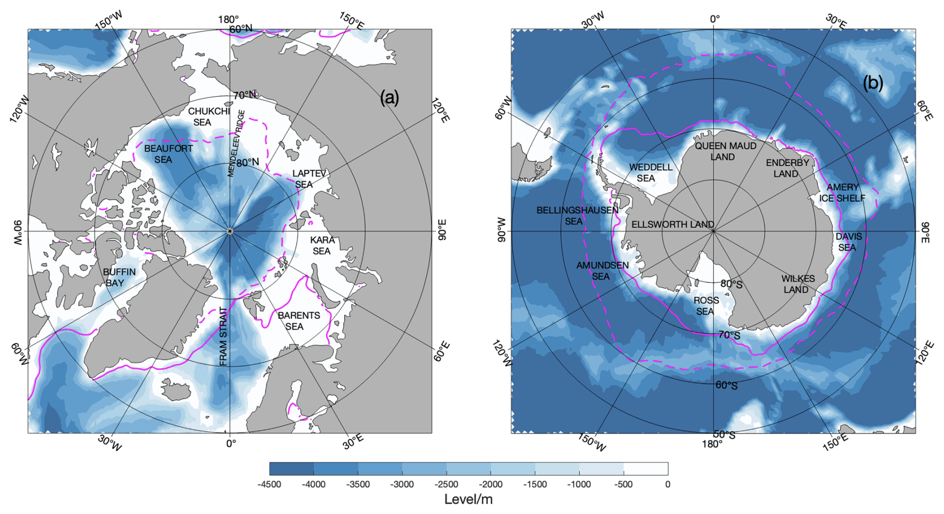
Figure 1 Study region in (a) Arctic Ocean and (b) Southern Ocean. Blue shading represents the bathymetry in meters. Solid and dashed magenta lines indicate the median sea-ice extent boundaries for March and September, respectively, defined by areas with sea-ice concentration.

Section 2 provides a description of the satellite datasets used and processing steps, along with the methods for calculating ocean-surface stress and Ekman circulation. Section 3 presents the time-mean patterns and variability of the derived surface stress and Ekman pumping fields. Section 4 addresses the quantification of uncertainties in the analysis, including sensitivity to the ice–water drag coefficient and comparisons with in situ data.

2 Data, method, and processing of the analysis

2.1 Calculation of ocean-surface stress and the Ekman transport

The ocean-surface stress is estimated using the methodology proposed by Yang (2006, 2009), with modifications by Meneghello et al. (2018). The total ocean-surface stress (τ_o) is calculated as a weighted linear combination of ice–water stress (τ_iw) and air–water stress (τ_aw), based on the fractional sea-ice concentration:

$$\begin{array}{}\text{(1)}& {\mathit{\tau }}_{\mathrm{o}}=\mathit{\alpha }{\mathit{\tau }}_{\mathrm{iw}}+(\mathrm{1}-\mathit{\alpha }){\mathit{\tau }}_{\mathrm{aw}},\end{array}$$

where α is set to 0 for the ice-free surfaces (defined as sea-ice concentration less than 15 %) and 1 for ice-covered surfaces (defined as sea-ice concentration exceeding 15 %). The stresses τ_iw and τ_aw are parameterized using quadratic drag laws:

$$\begin{array}{}\text{(2)}& {\mathit{\tau }}_{\mathrm{iw}}={\mathit{\rho }}_{\mathrm{w}}{C}_{\mathrm{D},\mathrm{iw}}\left|U_{\mathrm{ice}}-U_{\mathrm{e}}-U_{\mathrm{g}}\right|\left(U_{\mathrm{ice}}-U_{\mathrm{e}}-U_{\mathrm{g}}\right)\end{array}$$

and

$$\begin{array}{}\text{(3)}& {\mathit{\tau }}_{\mathrm{aw}}={\mathit{\rho }}_{\mathrm{a}}{C}_{\mathrm{D},\mathrm{aw}}\left|U_{\mathrm{10}}\right|U_{\mathrm{10}},\end{array}$$

where U_ice, U_e, U_g, and U₁₀ are the local ice motion, Ekman velocity, geostrophic velocity, and equivalent neutral wind at 10 m height, respectively; ρ_w= 1027.5 kg m⁻³ and ρ_a represent the densities of water and air, respectively. In this formula, τ_aw is taken directly from existing satellite wind products (Yu and Jin 2014a, b).

C_D,iw is the ice–water drag coefficient; $C_{\mathrm{D},\mathrm{iw}}=$ 5.5 × 10⁻³ is adopted in this product as it is a commonly recognized value. It is worth noting that, due to the limited availability of direct observations, C_D,iw is identified as a key source of uncertainty. A sensitivity analysis is therefore provided in the following section to evaluate its potential impact.

In Eq. (2), surface ocean velocity is expressed as the sum of U_g and U_e. The representation of ocean-surface stress is known to be highly sensitive to the assumed surface velocity used in the drag formulation. A range of approaches has been employed in past studies – incorporating U_e or U_g or even assuming zero ocean motion – each with markedly different implications. For instance, Zhong et al. (2018) showed that mean Ekman pumping in the Beaufort Sea can vary by over 50 %, depending on the inclusion of geostrophic flow. Wu et al. (2021) reported similar sensitivities in the Nordic Seas, while earlier works by Zhong et al. (2015) and Ma et al. (2017) further detailed the variability across Arctic regimes. As a result, stress-based diagnostics remain sensitive to parameterization choices, and conclusions should be interpreted with that uncertainty in mind.

The geostrophic velocity U_g can be calculated from dynamic ocean topography datasets (McPhee, 2013; Armitage et al., 2016, 2017). The Ekman velocity U_e, which moves at an angle of 45° to the right of the ocean-surface stress in the northern hemisphere, is calculated as

$$\begin{array}{}\text{(4)}& U_{\mathrm{e}}={\displaystyle \frac{\sqrt{\mathrm{2}}{\mathrm{e}}^{-\mathrm{i}(\mathit{\pi }/\mathrm{4})}}{f{\mathit{\rho }}_{\mathrm{w}}{D}_{\mathrm{e}}}}{\mathit{\tau }}_{\mathrm{o}},\end{array}$$

where f is the Coriolis parameter and D_e is the Ekman layer depth (20 m; Meneghello et al., 2018). Since U_e and τ_o are interdependent in Eqs. (1) and (4), a modified Richardson iteration method is applied to solve them iteratively until convergence is achieved, starting with U_e=0 in the first iteration (Yang, 2006).

Subsequently, the vertical Ekman velocity w_e can be calculated as follows:

$$\begin{array}{}\text{(5)}& w_{\mathrm{e}}={\displaystyle \frac{\mathrm{1}}{f{\mathit{\rho }}_{\mathrm{w}}}}\mathrm{\nabla }\times {\mathit{\tau }}_{\mathrm{o}}.\end{array}$$

A positive w_e indicates upwelling, while a negative w_e corresponds to downwelling.

2.2 Data description

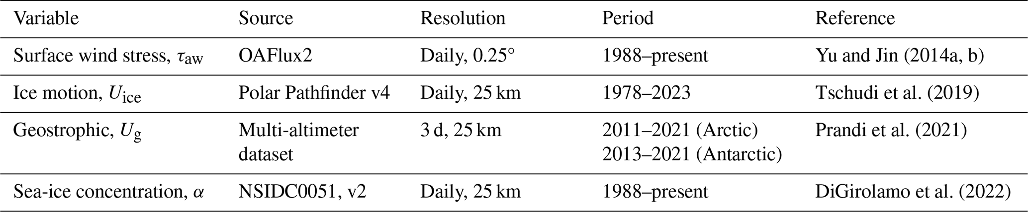
The calculation of total ocean-surface stress (Eqs. 1–4) requires the following input datasets: ocean-surface wind stress (τ_aw), sea-ice concentration (α), sea-ice motion (U_ice), and dynamic topography for geostrophic velocity (U_g). A brief description of each satellite-based dataset is given in Table 1.

Table 1 Gridded satellite datasets used in the work.

In this product, the air–water wind stress is taken from OAFlux2 (Yu and Jin, 2014a, b), a satellite-derived 0.25° gridded air–sea flux daily analysis (1988 to present) developed under the auspices of NASA's Making Earth System Data Records for Use in Research Environments (MEaSUREs) program (Yu, 2019). OAFlux2 winds are synthesized from 19 active and passive satellite wind sensors and wind stresses are calculated from the Coupled Ocean–Atmosphere Response Experiment (COARE) bulk algorithm, version 3.6 (Fairall et al., 2003).

Daily sea-ice motion vectors for the Arctic and Antarctic regions are obtained from the National Snow and Ice Data Center's (NSIDC's) Polar Pathfinder Daily 25 km EASE-Grid Sea-Ice Motion Vectors, version 4 (Tschudi et al., 2019, 2020), covering the period from 1978 through 2023. The ice motion fields are derived from multiple sources, including passive microwave radiometers (e.g., SSM/I, AMSR-E), visible and infrared sensors (e.g., AVHRR, MODIS), scatterometers (e.g., QuikSCAT), drifting buoys (e.g., IABP), and atmospheric wind reanalysis. Feature-tracking algorithms are applied to sequential satellite images to identify ice displacement, while optimal interpolation techniques combine the various data sources to produce daily sea-ice motion estimates. The resulting vectors represent sea-ice displacement over a 24 h period and are gridded onto a 25 km EASE grid 2.0 (EASE2).

Geostrophic velocity in the Arctic and Antarctic are obtained from the CLS/PML multi-altimeter combined Arctic/Antarctic Ocean sea-level dataset (Prandi et al., 2021). This dataset spans latitudes north of 50° N on a 25 km EASE2, with a temporal resolution of one grid point every 3 d. Covering the Arctic from 2011 to 2021 and the Antarctic from 2013 to 2021, the CLS dataset mitigates the spurious meridional signals often introduced by the longer sampling intervals of CryoSat-2 observations (Auger et al., 2022).

The sea-ice concentrations from Nimbus-7 SMMR and DMSP SSM/I-SSMIS Passive Microwave Data, version 2 (NSIDC-0051, Cavalieri et al., 1996; DiGirolamo et al., 2022) are used to define the daily ice boundary, based on the 15 % ice concentration threshold. NSIDC-0051 provides a reliable long-term record of sea-ice concentration, making it valuable for studying sea-ice conditions and large-scale climate variability (Parkinson, 2019). Widely recognized for its accuracy, the dataset is frequently used to validate and improve climate model simulations. The daily dataset is available from 1987 to the present and provides coverage for a 25 km resolution polar stereographic grid for both polar regions.

The analysis period ends in 2021 to maintain consistency with the most reliable iteration of the ongoing refinement of the associated satellite products, as listed in Table 1. While this choice limits the temporal extent, the framework itself remains flexible and can be readily extended as newer, better-resolved, datasets become available. With all considered, the study period for Antarctica is constrained to 6 years (2013–2021), while an 8-year period (2011–2021) is maintained for the Arctic.

2.3 Data processing procedure

Using the methodology described in Eqs. (1)–(5) and the input data listed in Table 1, the workflow for processing and analyzing data to calculate ocean-surface stress and derive vertical Ekman velocity is shown in Fig. 2.

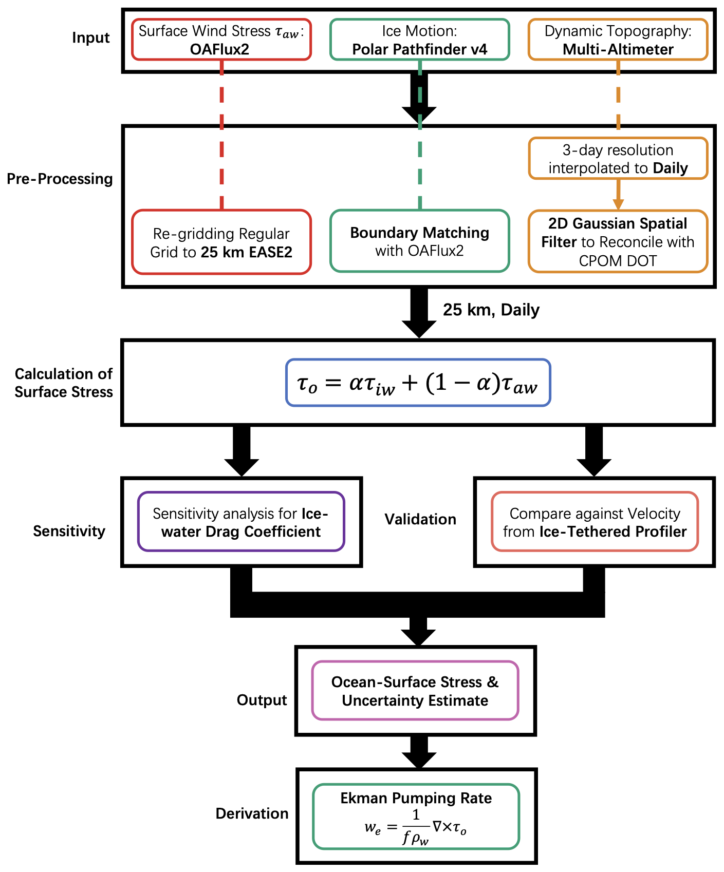
Figure 2 Workflow for data processing and analysis to calculate ocean-surface stress and derive vertical Ekman velocity.

All datasets are interpolated onto a common 25 km EASE grid format, providing uniform spatial resolution and facilitating consistent analysis across the Arctic and Antarctic regions. Note that the 25 km resolution may introduce uncertainties near the 15 % sea-ice concentration boundary, as such coarse resolution can obscure sharp gradients in the marginal ice zone and lead to misclassification of mixed ice–water grid cells (e.g., Meier, 2005; Ivanova et al., 2015).

Despite efforts to merge ice-edge boundaries across multiple satellite products, we note that data gaps and inconsistencies become more pronounced after 2019. This is primarily due to increasing divergence between input datasets used to define sea-ice concentration and motion. As a result, the quality of the derived surface stress fields may be reduced, particularly in the marginal ice zone (MIZ), where small changes in ice coverage can significantly affect stress partitioning. Users should exercise caution when applying this dataset to study MIZ dynamics after 2019; we recommend validating results against independent sources where possible.

Temporal sampling frequency plays a critical role in determining the accuracy and interpretability of ocean-surface stress estimates. Daily and sub-daily sampling is often needed to capture short-term variability in wind and sea-ice motion, which directly affects transient stress fluctuations and high-frequency Ekman responses (Meneghello et al., 2018; Regan et al., 2020). Conversely, monthly averaged fields may overly smooth dynamic features and obscure important stress events, particularly in regions with strong synoptic variability. In this context, the 3 d sampling of the CLS/PML altimetry product offers a useful compromise: it resolves large-scale mesoscale dynamics more consistently than monthly data while maintaining better signal-to-noise properties than noisy daily sea surface height reconstructions in ice-covered regions (Prandi et al., 2021). Given the limitations of satellite altimetry in the polar oceans, the CLS/PML dataset provides a crucial improvement by reducing spurious meridional errors and enabling more consistent estimation of geostrophic velocities and their role in modulating surface stress (Auger et al., 2022). We revisit the implications of time-averaging choices for surface stress/derived velocity fields in Sect. 4.2.

While the CLS/PML product offers improved temporal resolution and geophysical realism at finer spatial scales, its use of multiple altimeters and interpolation techniques can introduce high-frequency structures that remain difficult to validate, given the sparse in situ coverage at high latitudes (Prandi et al., 2021; Auger et al., 2022). In contrast, the CPOM dynamic ocean topography (DOT) dataset (2003–2021) from the Centre for Polar Observation and Modelling (CPOM; Armitage et al., 2016, 2017), despite its coarser resolution and monthly cadence, has seen wider adoption and validation across climate-scale Arctic studies (e.g., Meneghello et al., 2018; Zhong et al., 2018; Lin et al., 2023), making it a valuable benchmark for cross-comparison. To reconcile the strengths of both datasets, we apply a two-dimensional Gaussian spatial filter to smooth CLS/PML fields, aligning their effective resolution with CPOM and improving the interpretability of large-scale patterns. This hybrid approach leverages the temporal detail of CLS/PML while benefiting from the broader-scale reliability of CPOM, offering a more balanced foundation for stress estimation and error characterization in polar oceanographic applications.

We employed a 2D Gaussian filter with a standard deviation of 75 km to improve consistency and interpretability between CLS/PML and CPOM DOT datasets, which have different resolutions and small-scale characteristics. A sensitivity test was conducted to determine the optimal filter radius, ranging from 50 to 250 km. Smaller filters (e.g., <50 km) preserve small-scale variability but may complicate the interpretation of large-scale features, while larger filters (e.g., >250 km) can excessively smooth mesoscale processes, such as boundary currents, reducing a dataset's ability to capture key processes of polar dynamics.

To find the optimal filter size, a series of tests were conducted for 2011. The effectiveness of each filter setting was evaluated using the root mean square deviation (RMSD):

$$\begin{array}{}\text{(6)}& \mathrm{RMSD}=\sqrt{{\displaystyle \frac{\mathrm{1}}{N}}{\sum }_{i,j}(w_{{\mathrm{e}}_{i,j}}-w_{{\mathrm{e}}_{\mathrm{ref},(i,j)}}{)}^{\mathrm{2}}},\end{array}$$

where $w_{{\mathrm{e}}_{i.j}}$ represents the local vertical Ekman velocity w_e derived from the CLS dataset, filtered with a specific Gaussian filter size (e.g., 100, 150 km); $w_{{\mathrm{e}}_{\mathrm{ref},(i,j)}}$ is the reference vertical Ekman velocity calculated using the CPOM dataset; and N is the total number of the grid points with sea-ice coverage.

The unfiltered CLS/PML dataset exhibits clear seasonal variations in RMSD, with values peaking at 25 cm d⁻¹ during winter and decreasing in summer (Fig. 3a). Applying a Gaussian filter significantly enhances agreement with the CPOM dataset, reducing RMSD by 10–15 cm d⁻¹ for most of the year. However, in late summer the reduction is only 2–5 cm d⁻¹.

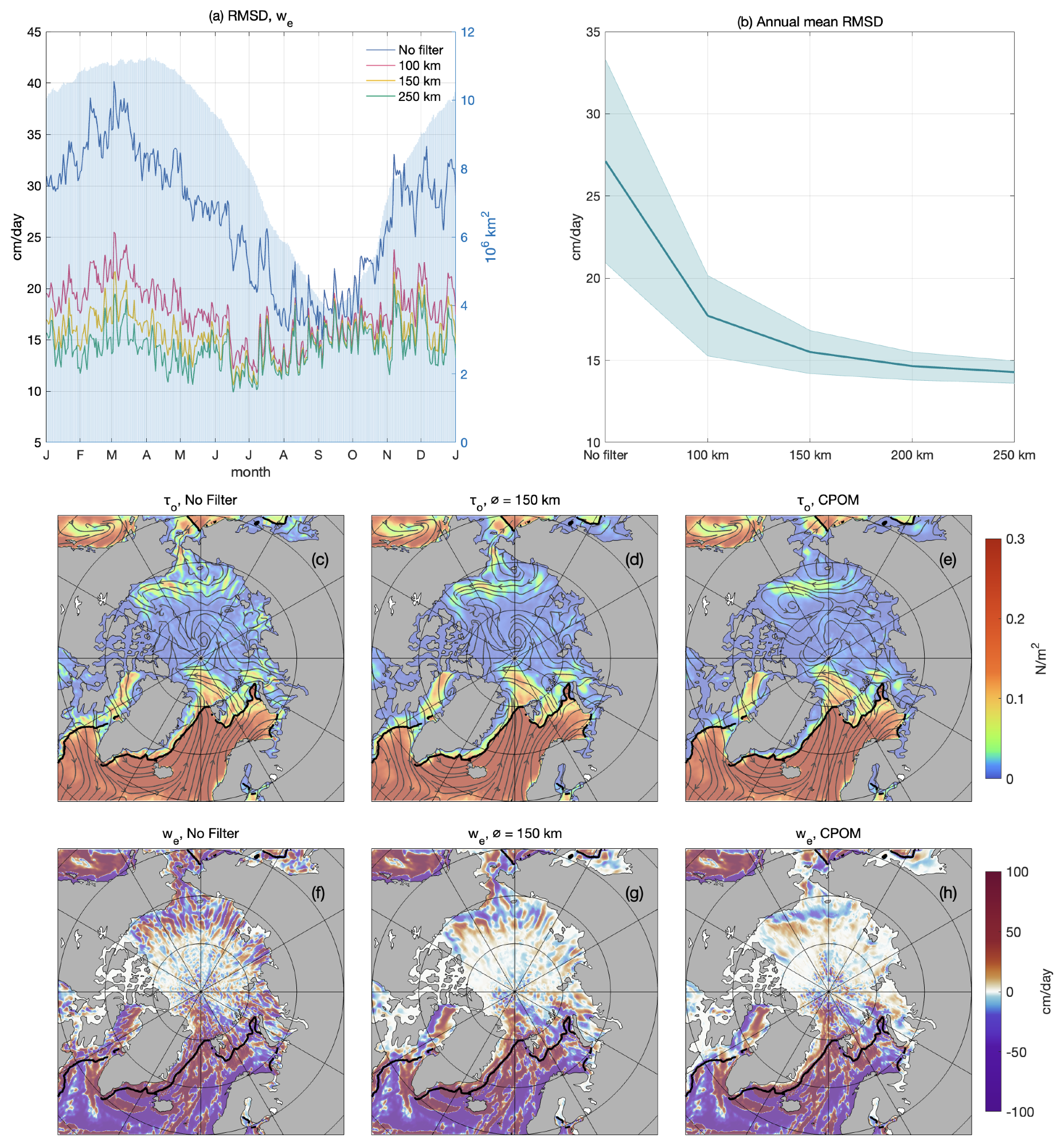
Figure 3 Area-averaged ocean-surface stress τ_o and vertical Ekman velocity w_e for different Gaussian filter settings. (a) Annual cycle of root mean square deviation (RMSD) of w_e over 2011. Blue shading shows total ice-cover areas (right axis). (b) Annual mean RMSD of w_e with shading indicating one standard deviation over a year. (c) Snapshot of τ_o with unfiltered CLS (15 March 2011). (d) Same as (c) but with 150 km Gaussian filter. (e) Same as (c) but with CPOM. (f)–(h) Same as (c)–(e) but for w_e. Streamlines in (c)–(e) show the direction of τ_o. Black contours in (c)–(h) mark 15 % ice concentration on 15 March 2011.

Increasing the filter size further enhances spatial agreement (Fig. 3b). From no filter to a 100 km filter, the annual mean RMSD is reduced to 17 cm d⁻¹; increasing the filter size to 150 km further lowers the RMSD to 15.5 cm d⁻¹. The standard deviation of daily RMSD is also reduced by half with a 150 km filter, compared with the unfiltered results. However, larger filter sizes (e.g., 200 and 250 km) yield only marginal additional improvements. Therefore, the 150 km Gaussian filter is selected as a practical and effective balance between preserving spatial features and minimizing small-scale variability for this work.

Figure 3c–h demonstrate the impact of varying filter size on the spatial structures of τ_o and w_e on 15 March 2011. Without filtering, the CLS dataset exhibits residual meridional striping due to satellite sampling artifacts (Auger et al., 2022). This pattern is significantly suppressed with a 150 km Gaussian filter. Between the filtered CLS-derived w_e (150 km) and CPOM-derived w_e, the correlation coefficients improve markedly from 0.77 (no filter) to over 0.95 (p<0.05).

3 Results and regional statistics

3.1 Arctic Ocean

In this section, we provide a concise overview of the surface stress and the corresponding Ekman velocity fields. Figure 4a shows the time-averaged ocean-surface stress (τ_o) field across the Arctic for 2011–2021. The highest τ_o appears in the ice-free Nordic Seas, where strong wind–ocean interactions drive surface stresses exceeding 0.3 N m⁻². In contrast, sea ice reduces momentum transfer and lowers τ_o in ice-covered regions. In the seasonal ice zone (SIZ), marked by the March and September sea-ice boundaries, τ_o typically remains below 0.05 N m⁻². Within the perennial ice zone (PIZ), bounded by the September sea-ice boundary, it drops further to below 0.02 N m⁻².

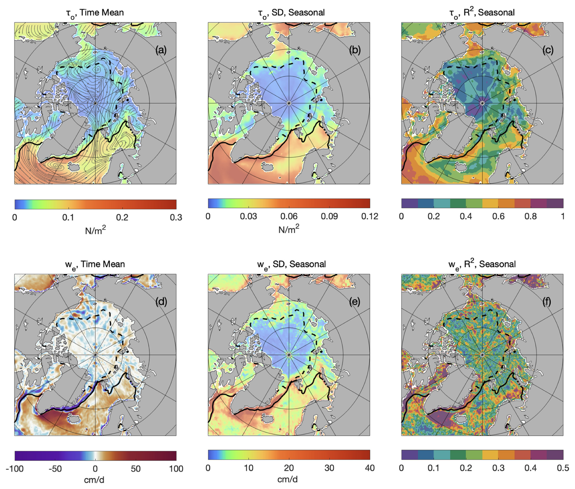
Figure 4 Mean and variability of ocean-surface stress τ_o and Ekman pumping rate w_e (positive indicates upwelling, negative indicates downwelling) in the Arctic region over 2011–2021. (a) Mean τ_o, with streamlines indicating the direction of stress. (b) Standard deviation of τ_o seasonal variability. (c) R², representing τ_o variance explained by seasonal variability. (d)–(f) Same as (a)–(c) but for w_e. The solid and dashed black lines represent the March and September sea-ice boundaries, respectively, defined by 15 % sea-ice concentration averaged over 2011–2021.

The seasonal cycle of τ_o is the dominant temporal variability across the Arctic (Stroeve and Notz, 2018). The standard deviation (SD) shows a spatial distribution similar to the time-averaged τ_o (Fig. 4b), with high variability (>0.1 N m⁻²) in ice-free regions like the Nordic Seas. Variability is significantly suppressed in the SIZ and PIZ, with values below 0.02 and 0.01 N m⁻², respectively. The coefficient of determination (R², here, is calculated as the proportion of variance explained by the seasonal cycle, i.e., $R^{\mathrm{2}}=\mathrm{1}-\left({\sum }_i\right(y_i-y_{\mathrm{seasonal}}{)}^{\mathrm{2}})/({\sum }_i(y_i-\stackrel{\mathrm{‾}}{y}{)}^{\mathrm{2}})$) shows that, in open-ocean regions, 40 %–60 % of variance is explained by seasonal variability (Fig. 4c). In ice-covered areas, this ratio drops to less than 30 %.

The time-mean Ekman pumping rate (w_e) and its SD and R² patterns are given in Fig. 4d–f. Strong upwelling (>50 cm d⁻¹) is observed in the Nordic Seas, while strong downwelling (<−10 cm d⁻¹) occurs in the Beaufort and Chukchi Seas. The spatial pattern of the SD of w_e is similar to that of τ_o (Fig. 4e). Seasonal variability ranges from 10–20 cm d⁻¹ in ice-free regions and 4–6 cm d⁻¹ in the SIZ, and falls below 4 cm d⁻¹ in the PIZ. Seasonal variability accounts for up to 60 % of w_e variance south of the Denmark Strait, but in other regions, including both ice-covered and ice-free zones, it typically explains 10 %–30 %.

The seasonal cycle of area-averaged wind–ocean-surface stress (τ_aw) is marked by strong values in winter, peaking around 0.4 N m⁻², and much weaker values in summer, dropping below 0.05 N m⁻² (Fig. 5a). This variation corresponds to the seasonal retreat of sea ice and the associated expansion of open ocean during summer months.

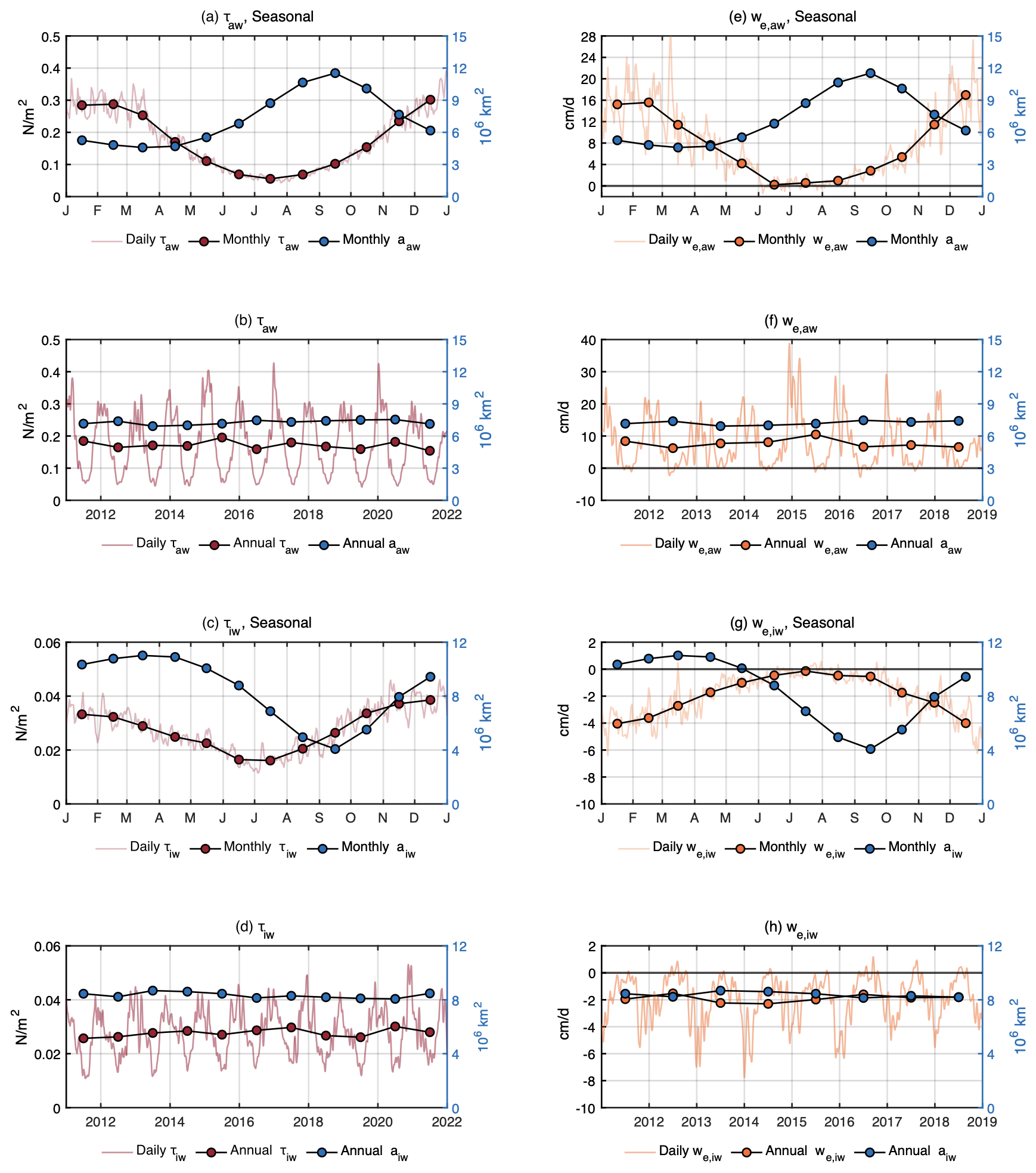
Figure 5 Mean seasonal cycle and annual time series of area-averaged surface stress τ_o (red) and Ekman pumping rate w_e (orange: positive indicates upwelling, negative indicates downwelling) for the Arctic region. Total areas a of the corresponding areal coverage are also plotted (blue). Variables are subscripted “aw” when averaged/summed over ice-free open ocean and “iw” when averaged/summed over ice-covered open ocean. Annual and monthly means are shown as dots in all panels. (a) Seasonal cycle of τ_aw over ice-free open ocean. (b) Time series of τ_aw from 2011–2021. (c) Seasonal cycle of τ_iw over ice-covered ocean. (d) Time series of τ_iw from 2011–2021. (e)–(h) Same as (a)–(d) but for w_e and 2011–2018.

In ice-covered regions, the seasonal cycle of ice–ocean-surface stress (τ_iw) is similar to that of τ_aw, though with significantly lower magnitudes (Fig. 5c). The seasonal peak of τ_iw is slightly higher in 2018 than 2013, increasing from 0.010 N m⁻² to nearly 0.018 N m⁻².

Due to the aforementioned uncertainties in sea-ice boundary delineation, we do not present an analysis of the average Ekman pumping rates w_e after 2018, as these estimates become highly sensitive to edge conditions and are thus dominated by boundary artifacts.

In ice-free regions, the average pumping rate w_e,aw peaks during winter upwelling, reaching around 30 cm d⁻¹, and transitions to weak downwelling during the summer (Fig. 5e). Annual variation in winter maximum upwelling rate is evident, with a notable decline to 10 cm d⁻¹ by late 2018 (Fig. 5f). In contrast, in ice-covered regions, w_e,iw is predominantly negative (Fig. 5g), although occasional summer upwelling events occur on daily scales. Notably, the winter downwelling rate has decreased from approximately −8 cm d⁻¹ in 2013–2014 to about −4 cm d⁻¹ by 2017 (Fig. 5h).

3.2 Southern Ocean

The spatial distribution of the time-mean τ_o in the Antarctic region is shown in Fig. 6a; τ_o exhibits a prominent circumpolar pattern. In ice-free regions, τ_o typically ranges from 0.2 to 0.3 N m⁻². In the SIZ, τ_o decreases significantly, falling to 0.04–0.06 N m⁻², with strong regional variability.

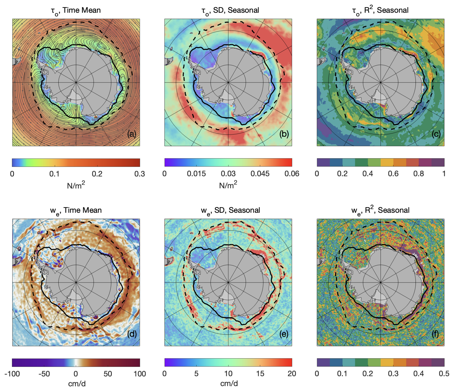
Figure 6 Mean and variability of ocean-surface stress τ_o and Ekman pumping rate w_e (positive indicates upwelling, negative indicates downwelling) in the Antarctic region over 2013–2021. (a) Mean τ_o, with streamlines indicating the direction of stress. (b) Standard deviation of τ_o seasonal variability. (c) R², representing τ_o variance explained by seasonal variability. (d)–(f) Same as (a)–(c) but for w_e. Streamlines in (a) show the direction of τ_o. The solid and dashed black lines represent the March and September sea-ice boundaries, respectively, defined by 15 % sea-ice concentration averaged over 2013–2021.

The SD of τ_o seasonal variability is evidently strong near the September sea-ice boundary, exceeding 0.1 N m⁻², particularly between 0 and 90° E (Fig. 6b). Moving northward into sub-polar open ocean, the SD gradually declines to approximately 0.04 N m⁻². Within the SIZ, seasonal variability diminishes further, typically ranging from 0.02 to 0.04 N m⁻². In the PIZ, it drops below 0.02 N m⁻². The value of R² shows that in such regions as the Indian Ocean and the southeast Pacific, seasonality explains over 50 % of the total variance, while in other areas this proportion ranges from 20 % to 40 % (Fig. 6c).

The spatial structure of the time-mean w_e reveals widespread upwelling south of 50° S (Fig. 6d), extending nearly all the way to the coast of Antarctica. In contrast to the Arctic, where strong ice–ocean coupling leads to clear transitions between upwelling and downwelling across ice boundaries, the Southern Ocean does not exhibit this distinct pattern. Downwelling is generally found around 55° S and farther north or more narrowly along the Antarctic coastline.

The SD pattern of seasonal variability in w_e is relatively consistent across the Southern Ocean (Fig. 6e), regardless of sea-ice coverage, with an average value of approximately 10 cm d⁻¹. Higher variability, reaching up to 20 cm d⁻¹, occurs only near the September ice boundary and is very localized. The R² pattern is also relatively homogeneous, with most areas showing seasonal variability accounting for about 30 % of the variance. Along the east coast of Antarctica, the seasonal cycle explains more than 50 % of the variance.

The seasonal cycle and time series of area-averaged air–water stress τ_aw in the Antarctic are shown in Fig. 7a and b. In ice-free regions of the Antarctic, the average τ_aw peaks in August at 0.36 N m⁻² and reaches its minimum in January at 0.13 N m⁻². Annual variability is relatively small, ranging between 0.022 and 0.026 N m⁻², with a notable positive anomaly in 2015, when the annual mean briefly increased to 0.028 N m⁻².

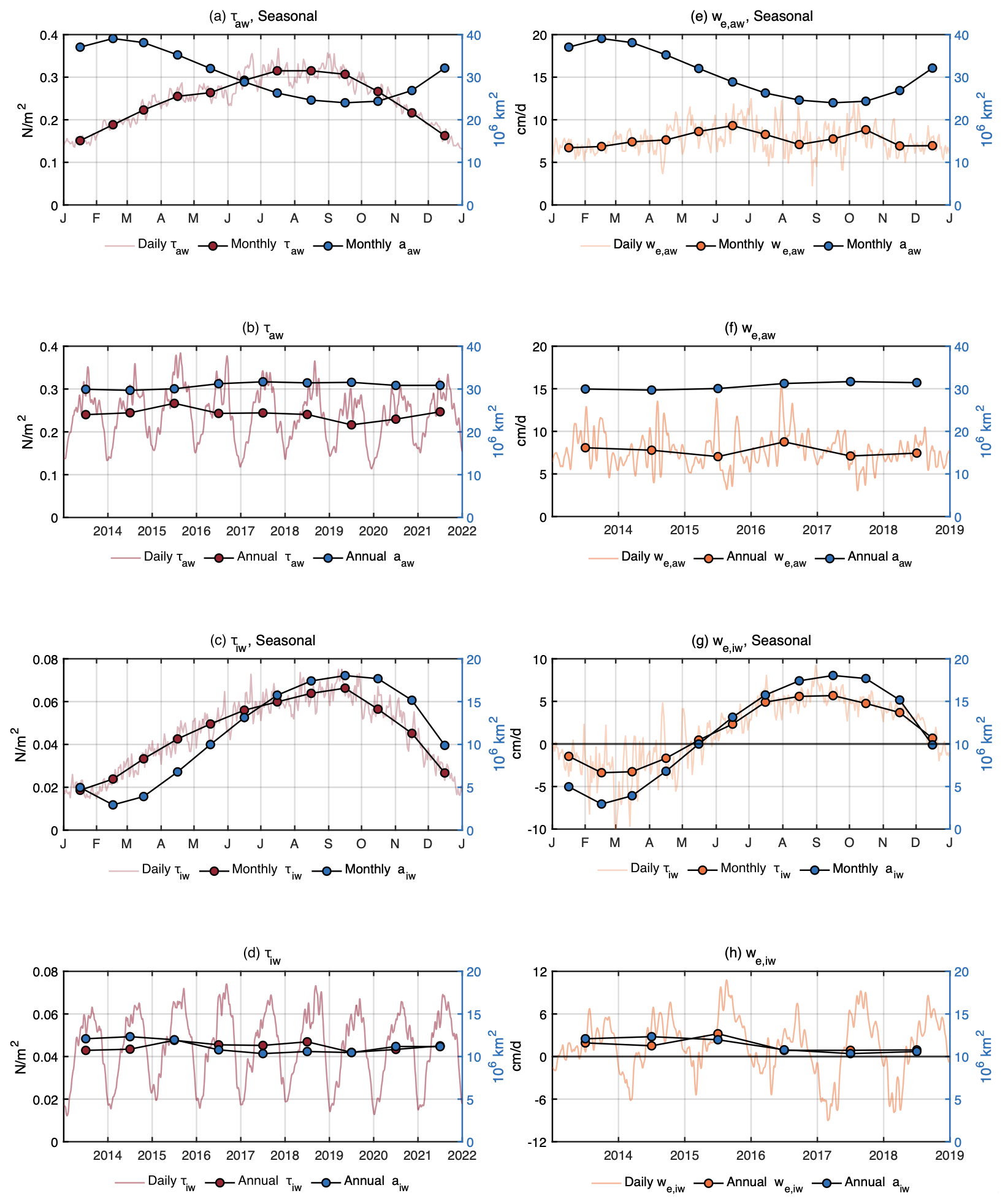
Figure 7 Time series and seasonal cycle of area-averaged surface stress τ_o (red) and Ekman pumping rate w_e (orange: positive indicates upwelling, negative indicates downwelling) for the Antarctic region. Total areas a of the corresponding areal coverage are also plotted (blue). Variables are subscripted “aw” when averaged/summed over ice-free open ocean and “iw” when averaged/summed over ice-covered open ocean. Annual and monthly means are shown as dots in all panels. (a) Seasonal cycle of τ_aw over ice-free open ocean. (b) Time series of τ_aw from 2013–2021. (c) Seasonal cycle of τ_iw over ice-covered ocean. (d) Time series of τ_iw from 2013–2021. (e)–(h) Same as (a)–(d) but for w_e and 2013–2018.

In ice-covered regions, ice–water stress τ_iw shows a delayed seasonal cycle, compared with τ_aw, and peaks in September (Fig. 7c). It is approximately one-fifth to one-half of τ_aw, ranging between 0.02 and 0.08 N m⁻². The seasonal pattern is asymmetrical and aligns with the seasonal cycle of sea-ice coverage (Eayrs et al., 2019). Similar to the Arctic, the area-averaged summer minimum of τ_iw is slightly higher in 2018, compared with 2013, increasing from 0.010 N m⁻² to 0.022 N m⁻².

Before 2019, the seasonal cycle of the open-ocean Ekman pumping rate w_e,aw is relatively weak (Fig. 7e), with higher values in winter (12 cm d⁻¹) and lower values in summer (5 cm d⁻¹). The absence of a distinct seasonal signal is probably due to the weaker seasonal cycle observed in 2017 and 2018 (Fig. 7f). The annual mean varies narrowly between 7 and 9 cm d⁻¹.

In ice-covered regions, w_e,iw is mostly positive throughout the year, with a brief downwelling period between January and April. A shift toward stronger downwelling occurs in February, with mean values decreasing from −2 cm d⁻¹ in 2013 to nearly −10 cm d⁻¹ by 2017. A notable anomaly occurred in 2015 when the annual mean rose sharply from 2 to 4 cm d⁻¹.

4 Uncertainty and data quality assessment

4.1 Sensitivity analysis of ice–water drag coefficient and uncertainty estimate

The ice–water drag coefficient, C_D,iw, is often assumed to be constant across time and space, due to the scarcity of direct observations that capture its spatiotemporal variability. However, C_D,iw can vary significantly, depending on environmental conditions, such as wind and wave dynamics, ice roughness, sea-ice concentration, and surface morphology (Lüpkes et al., 2012; Lüpkes and Birnbaum, 2005; Cole and Stadler, 2019). Reported values for C_D,iw range from 0.7 to over 10.0 × 10⁻³ (Overland, 1985; Guest and Davidson, 1987, 1991; McPhee, 2008; Cole et al., 2014), with some extreme cases reaching magnitudes of the order of 10.0 × 10⁻¹ (Kawaguchi et al., 2024).

Commonly, a representative value of 5.5 × 10⁻³ has been widely adopted as a pragmatic approximation by the scientific community (Guest and Davidson, 1987; Anderson, 1987). However, this approximation may overlook important spatial and temporal variations in C_D,iw, highlighting the need for ongoing efforts to improve observations and refine its parameterization.

To evaluate the sensitivity of estimated τ_o to the variations in C_D,iw, two sets of experiments are conducted for 2011: one with fixed C_D,iw values ranging from 1.0 × 10⁻³ to 10.0 × 10⁻³ and another using a randomized weighting map, dynamically varying C_D,iw between values of the order of 10⁻³ and 10⁻² on a daily basis at each grid cell.

The amplitude of τ_o scales proportionally with C_D,iw, as implied from Eq. (2) (Fig. 8a). For fixed coefficients, the summer mean τ_o increases from 0.003 N m⁻² at $C_{\mathrm{D},\mathrm{iw}}=$ 1.0 × 10⁻³ to 0.015 N m⁻² at $C_{\mathrm{D},\mathrm{iw}}=$ 10.0 × 10⁻³, while winter means rise from 0.012 to 0.053 N m⁻². Results from the random-weighted C_D,iw experiment closely follow the fixed cases of $C_{\mathrm{D},\mathrm{iw}}=$ 5.0–6.0 × 10⁻³. Similarly, the annual mean τ_o and its standard deviation increase proportionally with C_D,iw (Fig. 8b), quadrupling the annual mean and raising the standard deviation from 0.003 to 0.017 N m⁻² as C_D,iw increases.

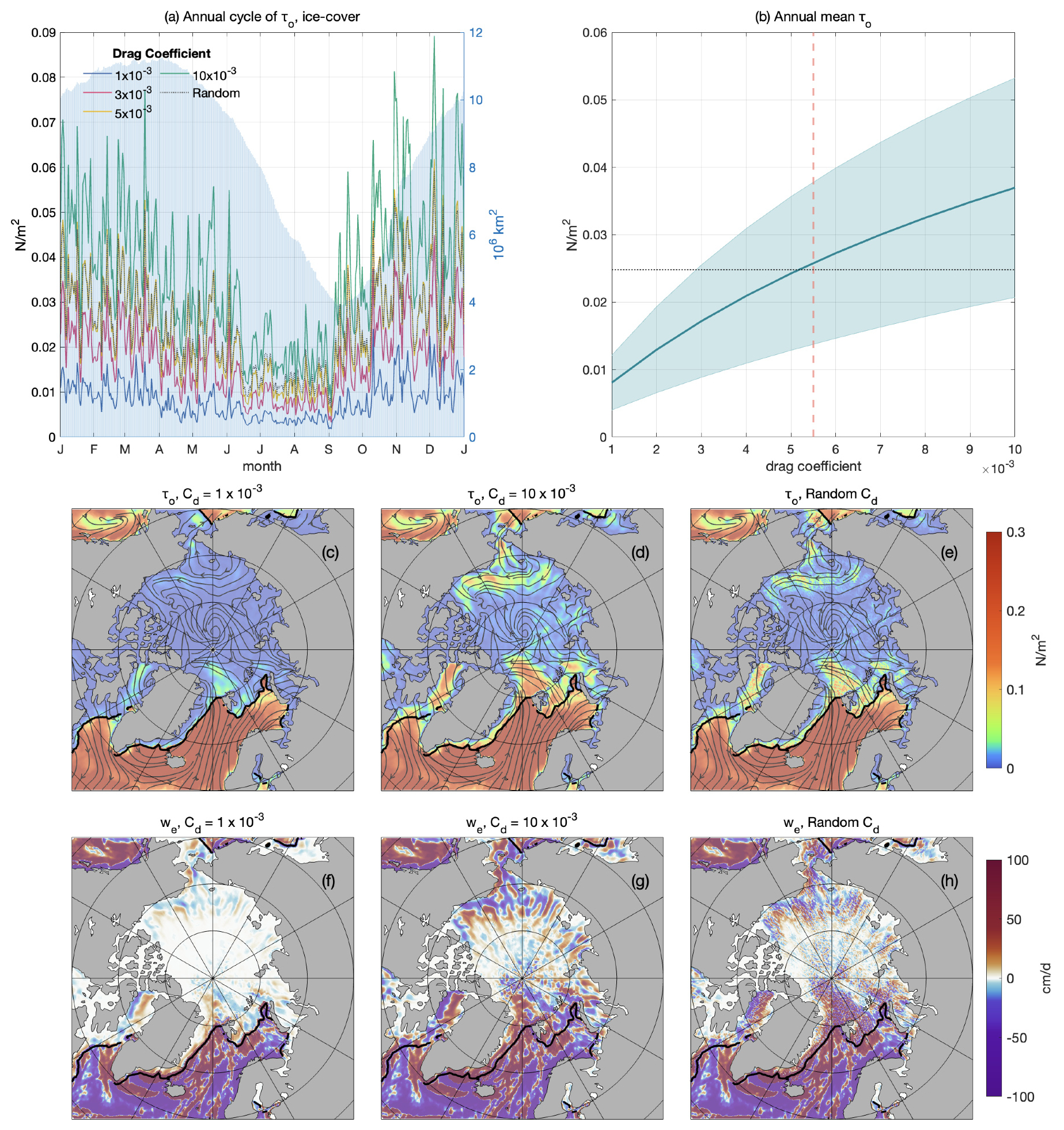
Figure 8 Area-averaged ocean-surface stress τ_o and Ekman pumping rate w_e for different values of C_D,iw. (a) Annual cycle of τ_o of 2011, area-averaged over the sea-ice-cover region. Blue areas show total ice-cover areas (right axis). (b) Annual mean of τ_o with shading indicating 1 standard deviation over a year. The red dashed line marks $C_{\mathrm{D},\mathrm{iw}}=$ 5.5 × 10⁻³; the black dotted line shows the annual mean of the random C_D,iw experiment. (c) Snapshot of τ_o with $C_{\mathrm{D},\mathrm{iw}}=$ 1.0 × 10⁻³ (15 March 2011). (d) Same as (c) but with $C_{\mathrm{D},\mathrm{iw}}=$ 10.0 × 10⁻³ . (e) Same as (c) but with random C_D,iw. (f–h) Same as (c)–(e) but for w_e. Streamlines in (c)–(e) show the direction of τ_o. Black contours in (c)–(h) mark the 15 % ice concentration on 15 March 2011.

Figure 8c–h show the spatial distribution of τ_o and w_e in response to varying C_D,iw. Under circumstances of low C_D,iw, momentum transfer between ice and ocean is reduced, leaving small and indistinct scale variability, particularly in the central Arctic. As C_D,iw increases, regions with high surface stress intensify, particularly in areas like Baffin Bay, the Chukchi Sea, and north of Fram Strait.

At $C_{\mathrm{D},\mathrm{iw}}=$ 1.0 × 10⁻³, the Ekman pumping rate in regions like the Fram Strait barely reaches ±8 cm d⁻¹, whereas at $C_{\mathrm{D},\mathrm{iw}}=$ 10.0 × 10⁻³, it exceeds ±30 cm d⁻¹, with strong contrasting upwelling and downwelling patterns. Additionally, while the random-weighted C_D,iw experiment introduces spatial noise, the broader spatial structures of both τ_o and w_e remain consistent with fixed-coefficient runs.

The final estimated uncertainty, ε_iw, in the ice–water stress τ_iw is quantified daily through the integration of standard errors from sensitivity analyses of C_D,iw and spatial Gaussian filter tests. Both filter tests and C_D,iw tests are extended to the full analysis period: 11 years (2011–2021) for the Arctic and 9 years (2013–2021) for the Antarctic. Using the root-sum-square method, the combined uncertainty is expressed as

$$\begin{array}{}\text{(7)}& {\mathit{\epsilon }}_{\mathrm{iw}}=\sqrt{{\left({\mathit{\epsilon }}_{\mathrm{iw},\mathrm{F}}\right)}^{\mathrm{2}}+{\left({\mathit{\epsilon }}_{\mathrm{iw},\mathrm{C}}\right)}^{\mathrm{2}}}=\sqrt{{\left({\displaystyle \frac{{\mathit{\sigma }}_{\mathrm{F}}}{\sqrt{N_{\mathrm{1}}}}}\right)}^{\mathrm{2}}+{\left({\displaystyle \frac{{\mathit{\sigma }}_{\mathrm{C}}}{\sqrt{N_{\mathrm{2}}}}}\right)}^{\mathrm{2}}},\end{array}$$

where σ_F is the standard deviation of τ_iw from different Gaussian filter settings and σ_C represents the standard deviation of τ_iw from sensitivity analysis on varying C_D,iw. The terms N₁ and N₂ denote the number of runs performed in each sensitivity analysis. This estimate assumes independence between C_D,iw and geostrophic fields (which were spatially filtered), with perturbations of comparable amplitude between the two sets of sensitivity analyses.

Figure 9 shows the spatial distributions of relative uncertainty (ε_iw to τ_iw) for the Arctic (15 March 2013) and the Southern Ocean (15 September 2013) during the winter season. Overall, spatial filtering produces scattered patterns (Fig. 9a–d), while varying ice–water drag coefficients yield smoother distributions (Fig. 9e–h). Median uncertainties are comparable between the two sets of experiments, ranging from 14 %–18 % in the Arctic to 22 %–25 % in the Antarctic. The greater uncertainties in the Antarctic reflect higher local stress variability and increased sensitivity to parameter changes, which also manifest as the higher uncertainties observed in winter, compared with summer (Figs. 3 and 8).

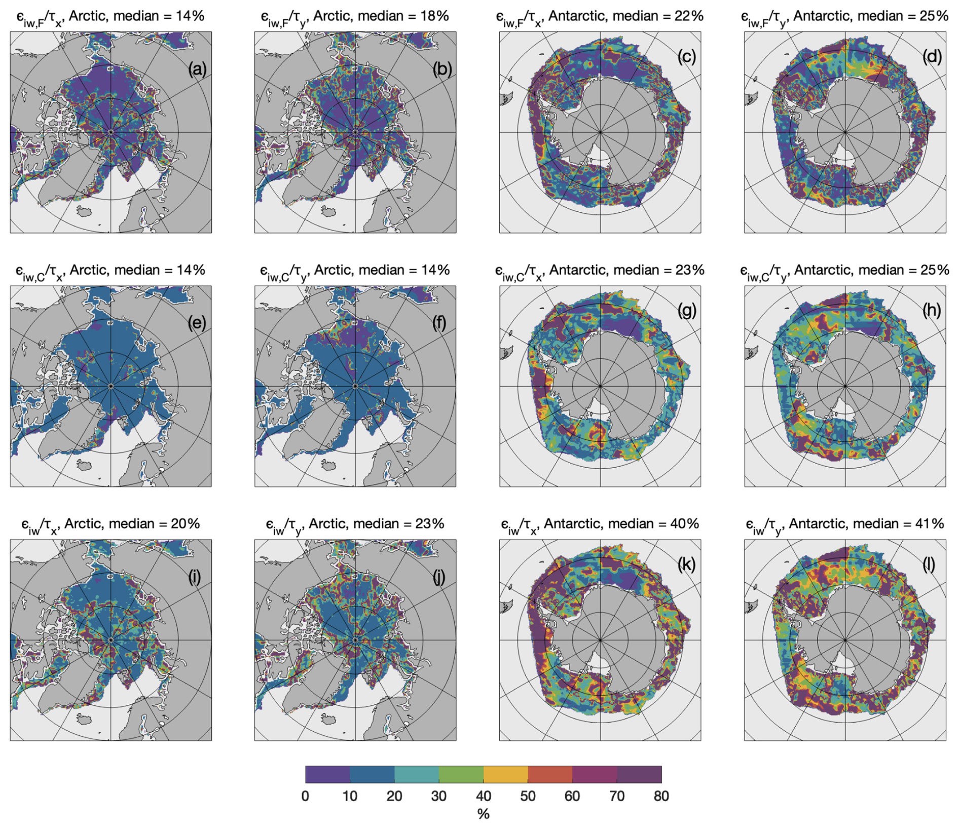
Figure 9 Estimated uncertainty fields for zonal and meridional ice–water surface stress, expressed as a ratio to the estimated ice–water surface stress in the Arctic (15 March 2013) and Southern Ocean (15 September 2013). (a) Standard error introduced by Gaussian filter in the Arctic, zonal direction. (b) Error from filter in the Arctic, meridional direction. (c, d) Same as (a, b) but for the Antarctic. (e)–(h) Same as (a)–(d) but for standard error in ice–water drag coefficient C_D,iw. (i)–(l) Same as (a)–(d) but for the combined uncertainty.

In the Arctic, combined uncertainties for zonal surface stress (τ_x) typically range from 10 %–20 %, while locally they could exceed 100 % along dynamic regions, such as the Fram Strait and Beaufort Sea. Meridional stress (τ_y) exhibits similar spatial distributions, but with higher uncertainties near the Mendeleev Ridge. Median uncertainty levels for both zonal and meridional components are below 20 %.

Conversely, Antarctic uncertainties are substantially higher, with median values around 40 %. The highest uncertainties (>60 %) are concentrated near the sea-ice boundary, particularly in the eastern Weddell and Ross Seas. Regional hotspots include the Antarctic Peninsula and west of Ross Sea for τ_x, and Enderby Land and the Amundsen Sea for τ_y.

In addition to the sensitivity analyses presented for drag coefficient magnitudes and spatial filtering, several other sources of uncertainty may influence the accuracy of the derived surface stress fields. First, uncertainties in the atmospheric reanalysis products used as forcing data – particularly in wind speed and direction over sea ice – can propagate directly into surface stress estimates. Prior studies have shown that different ice motion products can yield differences of at least 20 %–30 % in polar regions, due to discrepancies in boundary-layer representation, data assimilation techniques, and satellite retrieval biases (Sumata et al., 2014; Wang et al., 2022). These differences are especially pronounced in the marginal ice zone, where sharp gradients in atmospheric and surface properties are common (Wang et al., 2021; Boutin et al., 2020).

Second, the role of ocean and atmospheric stratification is not explicitly resolved in our parameterization, yet it can significantly affect stress transmission through the ice–ocean interface. Observational and modeling studies (Lüpkes and Gryanik, 2015; Lüpkes et al., 2012; Brenner et al., 2021) have shown that stability conditions in the atmospheric boundary layer modulate drag coefficients by altering turbulence and momentum fluxes – especially under stable stratification, common in winter Arctic conditions. Likewise, vertical stratification in the upper ocean can modify Ekman layer dynamics and the effective depth over which stress-induced velocities operate, introducing further uncertainty in estimates of vertical transport (Meneghello et al., 2018; Zhong et al., 2018).

Third, the spatial and temporal scales over which stresses are calculated can introduce methodological uncertainty. Coarse averaging may obscure high-frequency processes, such as synoptic wind events, inertial motions, or mesoscale eddies, while finer-scale estimates risk amplifying local noise or aliasing undersampled variability (Timmermans et al., 2008; Manucharyan and Thompson, 2017; Alberello et al., 2020). This is particularly relevant in the marginal ice zone, where surface properties evolve rapidly. A more detailed analysis of scale effects and filtering sensitivity is presented in the following section.

Together, these factors point to the need for caution when interpreting surface stress magnitudes or derived quantities like Ekman pumping, particularly when used to constrain physical budgets or force ocean models. Future work should prioritize uncertainty quantification through ensemble reanalysis comparisons, the inclusion of stratification effects in drag parameterizations, and adaptive filtering techniques that respond to local dynamic conditions.

4.2 Validation with ITP observations

Since surface stress is not usually directly measured, assessing the performance of our analysis is challenging. To address this, we revisit the assumption that surface velocity comprises both Ekman and geostrophic components, as described in Eq. (2). The geostrophic velocity (U_g) is derived from the dataset provided by Prandi et al. (2021), while the Ekman velocity component (U_e) can be easily calculated from the ocean-surface stress using Eq. (4).

This assumption provides a first-order approximation of surface velocity and neglects other processes, such as ageostrophic motions, vertical shear, and sub-mesoscale dynamics, which may introduce additional uncertainties. To robustly validate satellite-derived ocean-surface stress estimates, we compared the derived surface velocity, i.e., the sum of U_g and U_e, with in situ measurements from ice-tethered profilers (ITPs; Krishfield et al., 2008; Toole et al., 2011; http://www.whoi.edu/itp, last access: 30 May 2025). In particular, several ITPs equipped with velocity sensors (ITP-V, Williams et al., 2010) were used. To align the temporal resolution of the datasets, we processed the ITP data by computing daily and weekly means, facilitating direct comparisons with daily satellite products. This approach avoids the uncertainties associated with interpolating satellite data to match the higher-frequency ITP profiles, which could introduce significant errors due to the undersampling nature of satellite observations.

Despite this temporal alignment, inherent limitations persist, due to spatial and temporal sampling discrepancies. ITPs provide high-resolution vertical profiles at specific locations, capturing fine-scale and transient oceanic features. In contrast, satellite observations offer broader spatial coverage but may not resolve such fine-scale variability, especially in polar regions, where data gaps are common due to persistent cloud cover and sea ice. These differences can lead to reduced correlation and increased bias in validation statistics, as observed in previous studies comparing satellite-derived sea-surface salinity products with in situ observations (Thouvenin-Masson et al., 2022; Boutin et al., 2016; Vinogradova and Ponte, 2013).

It is important to note that this comparison does not serve as a definitive validation of the absolute accuracy of our stress estimates. Instead, it assesses whether the foundational assumptions underpinning our analysis sufficiently represent the complex dynamics of the Arctic Ocean.

We use velocity data collected from five ITP-V missions deployed on multiyear sea ice in the Canada Basin between 2011 and 2019 (Fig. 10; Table 2). Observations from ITP-77, ITP-78, and ITP-79 are truncated to exclude periods with significant data gaps and drifts near the end of their deployment.

Table 2 Details of ITP-V records.

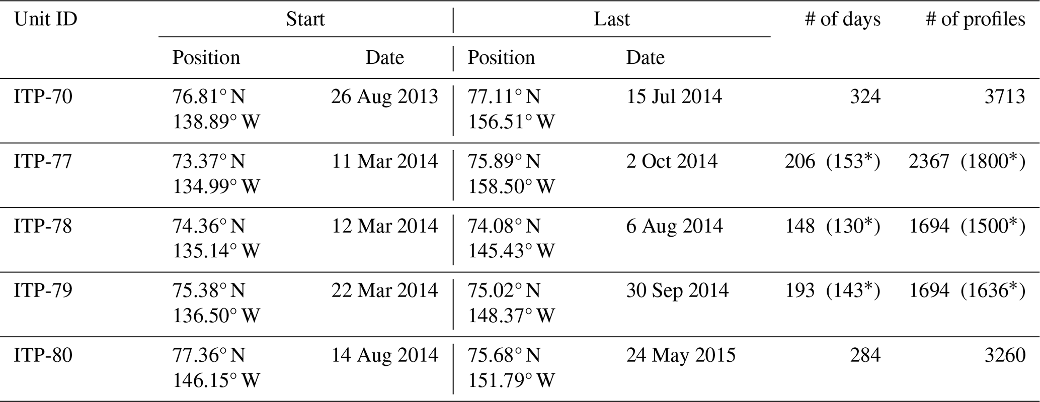
^* Data toward the end of the series exhibit quality issues that necessitate truncation.

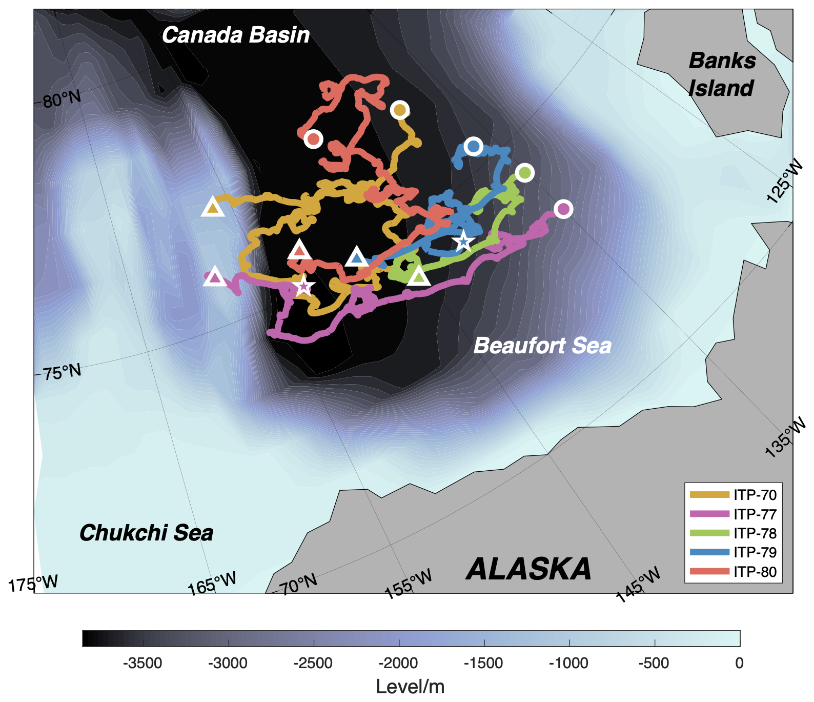
Figure 10 ITP-V drift paths in the Arctic Ocean (colored curves). Deployment locations are marked by circles, latest locations by triangles, and the cutoff locations for ITP-77 and ITP-79 by stars.

The five ITP-Vs are categorized into two groups, based on deployment timing and drift trajectories. ITP-70 and ITP-80 were deployed during summer, operated for ≈300 d, and primarily drifted between 75 and 80° N. In contrast, ITP-77, ITP-78, and ITP-79, deployed in March 2014, operated for less than 200 d and followed more constrained east-to-west trajectories between 73 and 75° N.

To account for temporal sampling differences and mitigate aliasing from high-frequency variability, the sub-daily ITP-V velocity data are first averaged to daily means before comparison with the satellite-derived velocity field (U_g+U_e). The corresponding satellite values are then extracted at the nearest grid point along each ITP track (Fig. 11). This approach reduces mismatch due to sub-sampling in the satellite product and ensures a more consistent temporal basis for comparison.

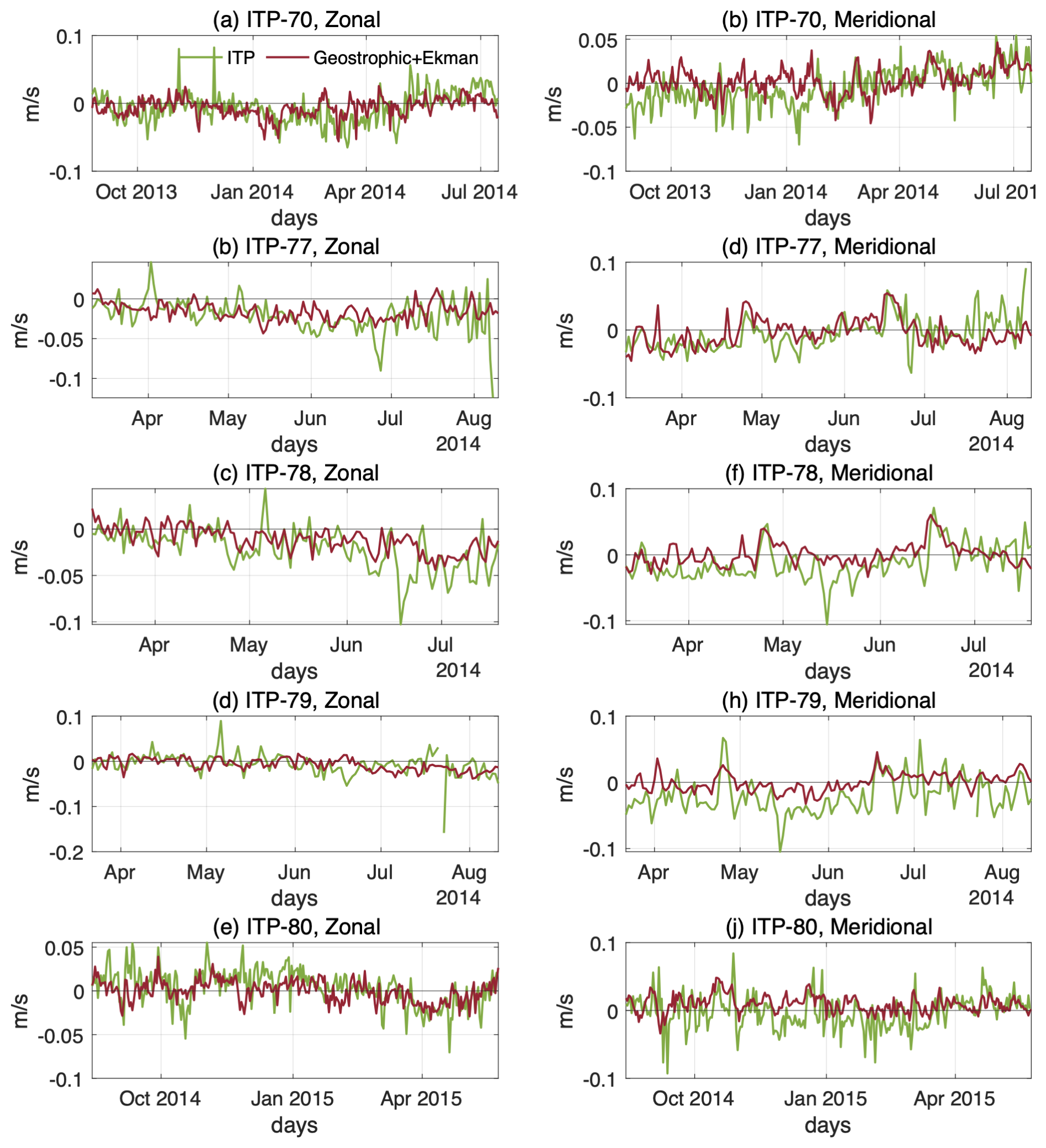
Figure 11 Daily mean time series of zonal and meridional surface velocity. (a) Zonal velocity along ITP-70 paths. (b) Zonal velocity along ITP-77 paths. (c) Zonal velocity along ITP-78 paths. (d) Zonal velocity along ITP-79 paths. (e) Zonal velocity along ITP-80 paths. (f)–(j) Same as (a)–(e) but for meridional velocity. Green curves represent velocity data retrieved from ITPs. Red curves are collocated obtained from the satellite-derived velocity fields, i.e., geostrophic plus Ekman velocity.

Along the path of ITP-70 and ITP-80, satellite-derived ocean-surface velocities exhibit moderate agreement with in situ observations, particularly in capturing high-frequency variability. In contrast, comparisons with ITP-77, ITP-78, and ITP-79 reveal weaker correspondence, most notably in the zonal velocity components. For the meridional component, ITP-77 shows relatively better alignment during the initial ≈100 d period until mid-July.

Figure 12 presents the comparison of satellite-derived surface velocity components against collocated ITP-V observations for the ITP-70 (panels a, b) and ITP-80 (panels c, d) paths. For ITP-70, the zonal component yields a Pearson correlation of r= 0.31 and standard deviation of 0.022 m s⁻¹, while the meridional component gives r= 0.42 and SD = 0.020 m s⁻¹. ITP-80 exhibits slightly stronger zonal agreement (r= 0.43) but weaker meridional agreement (r= 0.34). In both deployments, scatter markedly decreases for observations taken after ≈200 d (warm colors), accompanied with the predominantly northward drift of ITP-70 and westward drift of ITP-80 seen in Fig. 10.

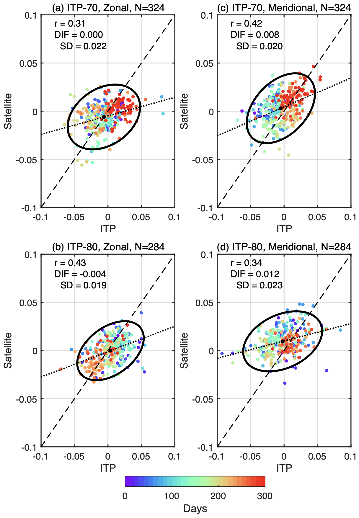
Figure 12 Scatterplots of collocated surface velocity pairs for ITPs with data spanning more than 200 d (unit: m s⁻¹). (a) Zonal velocity along ITP-70 paths. (b) Zonal velocity along ITP-80 paths. (c, d) Same as (a, b) but for meridional velocity. The total number of days (N) is given. Correlation coefficients, mean differences (DIF), and standard deviations (SD) of the differences between satellite-derived velocity and ITP observations are also displayed. 95 % confidence ellipses (black contours) and linear fits (black dotted lines) are also given in each panel.

By contrast, Fig. 13 summarizes the additional ITP observational periods (panels a–f), where correlation coefficients span r= 0.07–0.56 and SD = 0.021–0.025 m s⁻¹. One component reaches a moderate correlation (r= 0.56), while most remain weak (r<0.40); no coherent temporal clustering is apparent. Across all deployments, satellite-derived velocities exhibit a slight northward bias and tend to underestimate ITP-measured surface speeds beyond 100 d post-release.

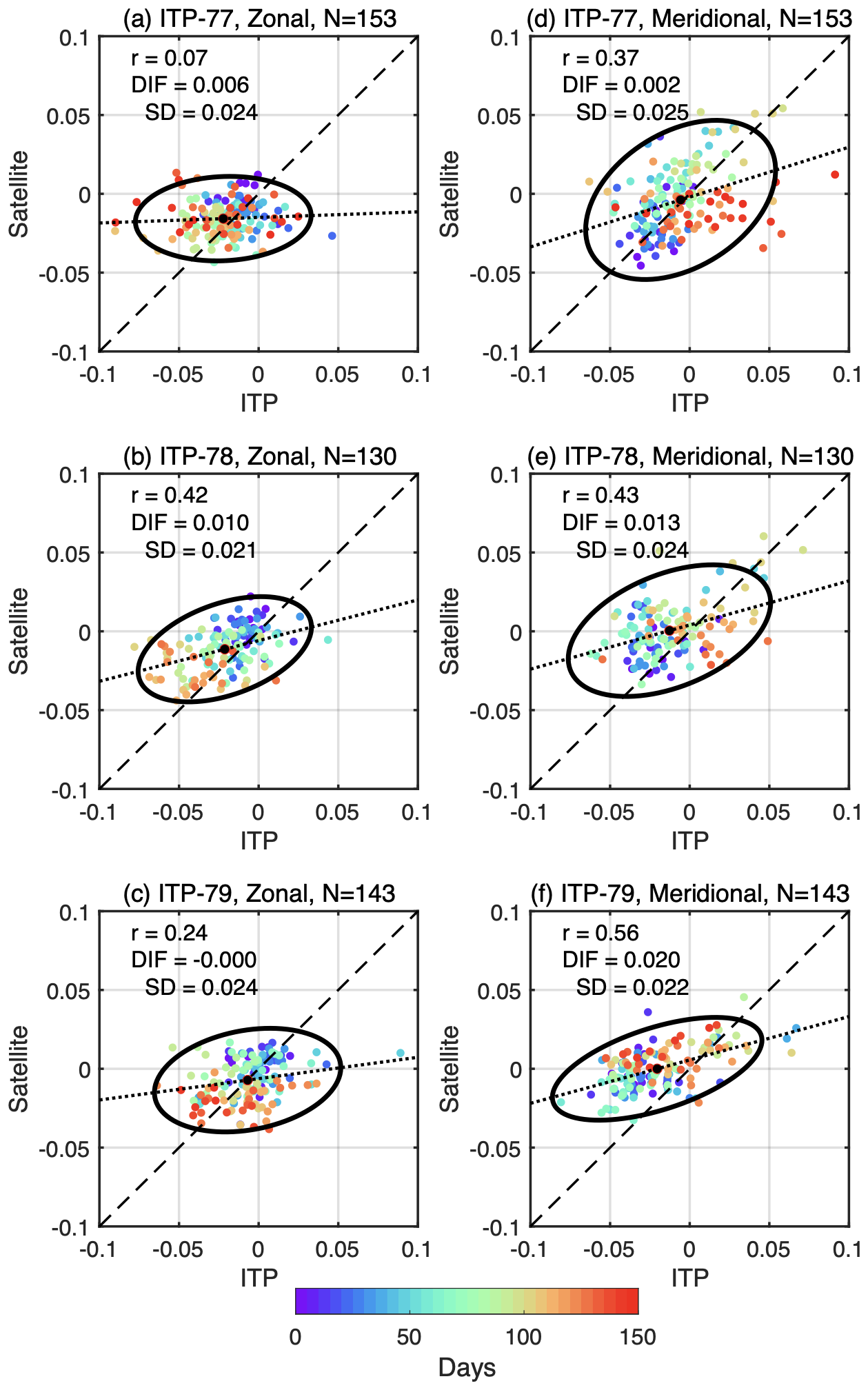
Figure 13 Scatterplots of collocated surface velocity pairs for ITPs with data spanning less than 200 d (unit: m s⁻¹). (a) Zonal velocity along ITP-77 paths. (b) Zonal velocity along ITP-78 paths. (c) Zonal velocity along ITP-79 paths. (d)–(f) Same as (a)–(c) but for meridional velocity. The total number of days (N) is given. Correlation coefficients, mean differences (DIF), and standard deviations (SD) of the differences between satellite-derived velocity and ITP observations are displayed. 95 % confidence ellipses (black contours) and linear fits (black dotted lines) are also given in each panel.

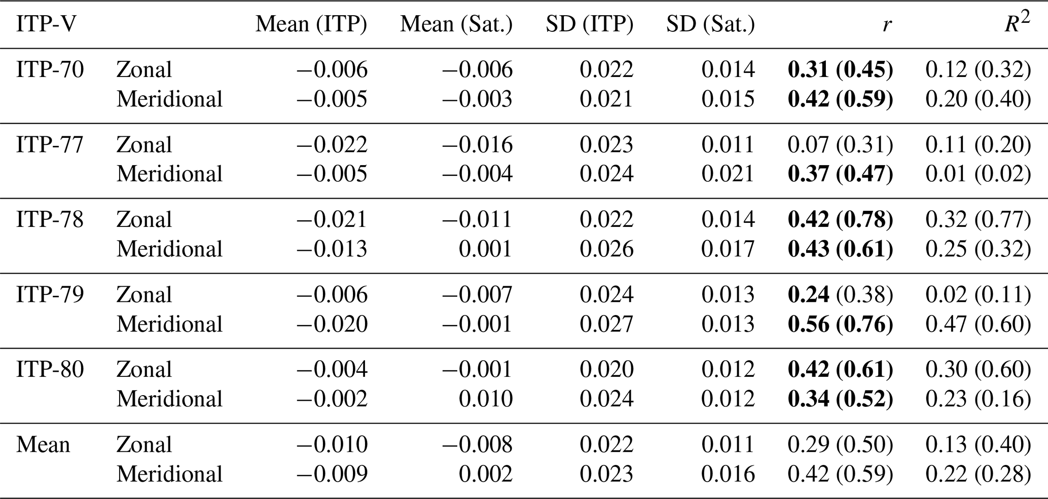
Table 3 and Fig. 14 provide a comprehensive comparison between satellite-derived surface velocity estimates and in situ velocity measurements obtained from ITP-V across five deployments. The analysis includes both the zonal (east–west) and meridional (north–south) velocity components and considers statistics derived from both daily and weekly averaged time series.

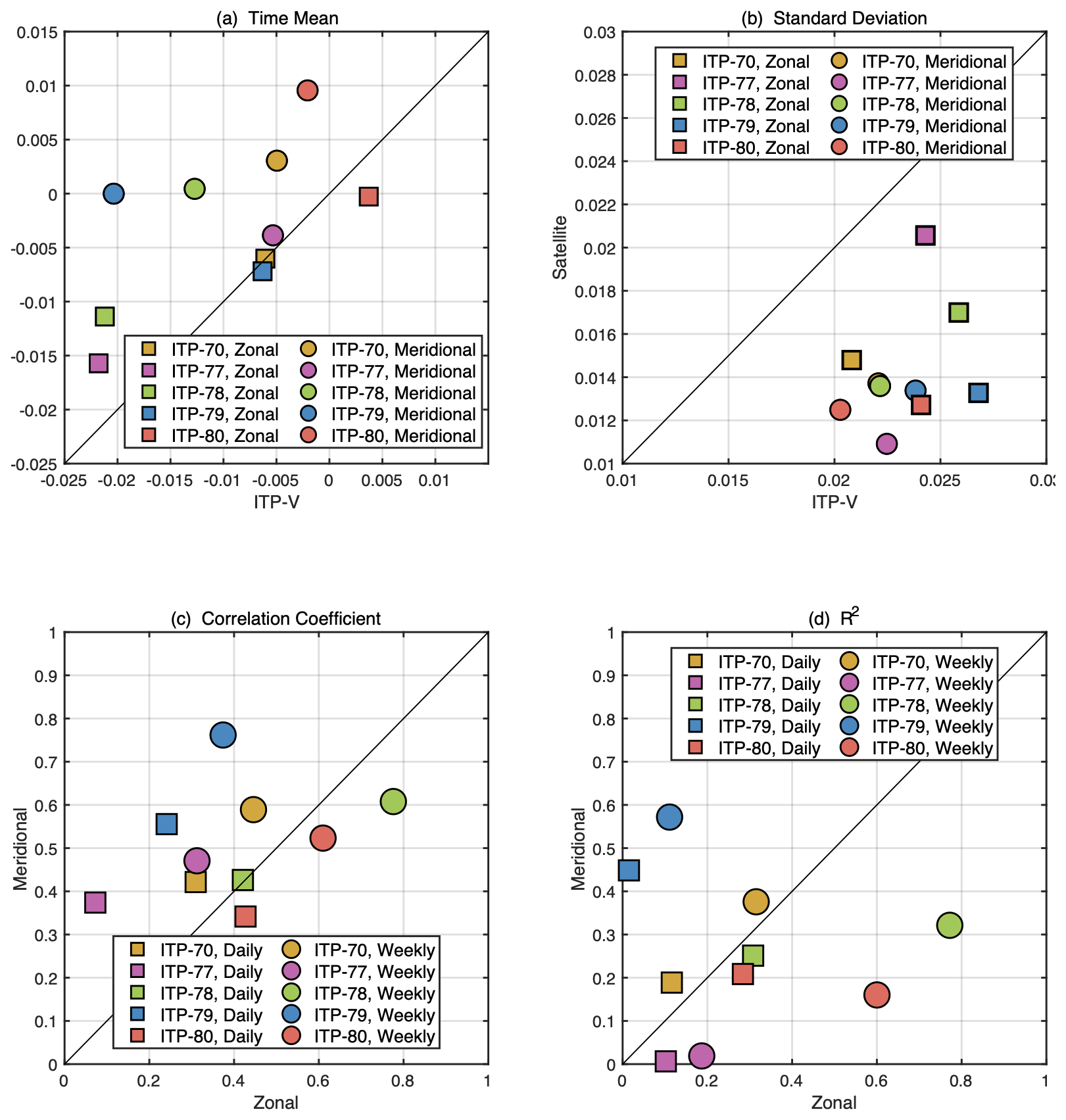
Figure 14 Scatterplots of statistics of satellite-derived velocity and ITP velocity. (a) Temporal mean and (b) standard deviation of paired velocities (unit: m s⁻¹). (c) Correlation between satellite-derived velocity and ITP velocity. (d) Coefficient of determination (R²) of variation in ITPs, explained by satellite-derived velocity.

A consistent northward bias is evident in the satellite-derived velocities across most ITP paths. While the mean zonal velocities are generally in close agreement between satellite and ITP-V data – for instance, at ITP-70 both sources report a mean of −0.006 m s⁻¹ – some deployments exhibit a more pronounced bias. ITP-77 and ITP-78, in particular, show a noticeable eastward offset, with satellite-derived zonal velocities being more positive than the ITP-V counterparts by approximately 0.005–0.01 m s⁻¹. The meridional component aligns more closely overall, but satellite velocities still tend to be more northward. These biases are evident in Fig. 14a, where most points lie above the 1:1 line, especially in the meridional direction.

In addition to the bias, satellite-derived velocities systematically exhibit reduced variability, compared with ITP-V observations. Across all deployments and components, the SD of satellite velocity is consistently lower than that observed in the ITP-V data. For example, while the average zonal SD in the ITP data is around 0.022 m s⁻¹, the corresponding satellite value is approximately 0.011 m s⁻¹. Figure 14b illustrates this discrepancy clearly: all data points fall below the 1:1 line, indicating that satellite products underestimate temporal variability. This reduced variability probably reflects the filtering and smoothing inherent in satellite altimetry products, which are designed to represent large-scale geostrophic flows and may not fully resolve the higher-frequency or smaller-scale fluctuations captured by the ITP instruments.

Despite these limitations, satellite-derived velocity fields are able to explain a substantial portion of the observed variance in the ITP-V measurements on a daily mean scale. The coefficients of determination (R²) indicate that, on average, satellite products account for about 50 % of the variability in the daily data. This explanatory power increases substantially when the analysis is performed on weekly averaged time series, with R² reaching as high as 0.77 for the zonal component at ITP-78 and 0.60 for the meridional component at ITP-79. These results suggest that, although satellite estimates smooth out finer-scale variability, they effectively capture the dominant patterns in large-scale motion. However, the correlation coefficients between satellite and ITP-V velocities are more modest, typically ranging from 0.3 to 0.4 in the daily records. With weekly averaging, these correlations improve significantly, sometimes by more than 0.2, as illustrated in Fig. 14c. This panel shows weekly averaged points clustering nearer to or above the diagonal, particularly for ITP-78 and ITP-79, while daily correlations tend to remain lower and more scattered.

The performance of the satellite velocity estimates varies by deployment. ITP-78 and ITP-79 demonstrate the strongest agreement. For example, ITP-78's zonal component yields correlation coefficients of 0.42 for daily data and 0.78 for weekly data, with R² values of 0.32 and 0.77, respectively. Similarly, ITP-79's meridional component shows a daily correlation of 0.56 and a weekly correlation of 0.76, with corresponding values of R² of 0.47 and 0.60, respectively. These high values underscore the ability of satellite altimetry to capture meaningful geophysical signals under favorable conditions. Conversely, performance is notably weaker at ITP-77, where the zonal velocity component yields a daily correlation of only 0.07 and a weekly correlation of 0.31, suggesting a diminished ability of satellite products to resolve local variability in that particular region or time frame. Such differences probably arise from a combination of regional oceanographic complexity and satellite data limitations, including issues related to proximity to sea ice or the presence of sub-mesoscale activity not well resolved by gridded products.

Table 3 Comparison of daily satellite-derived velocity with ITP velocity along ITP tracks. Correlations (r) with p<0.05 are in bold. Numbers in brackets are from weekly mean time series.

The comparison between satellite-derived ocean-surface stress estimates and ITP observations, despite their differences in resolution and sampling, shows encouraging agreement at the first-order level. The satellite stress products successfully capture the broad spatial and temporal variability in surface velocity, supporting the utility of satellite-based estimates in reflecting first-order dynamic signals. This level of agreement supports the overall utility of satellite products in characterizing large-scale stress variability and motivates their continued use in data-sparse polar regions.

However, key limitations remain, due to inherent mismatches in spatial and temporal sampling between the datasets. Satellite observations, with their typical resolution of ≈25 km and daily sampling frequency, cannot resolve the sub-mesoscale variability and high-frequency processes detectable in the pointwise and often sub-daily ITP profiles (Timmermans et al., 2008). This spatial averaging can smooth out gradients in wind, ice motion, or stress fields that may be sharply defined at smaller scales, particularly in such regions as the marginal ice zone (MIZ), where sea-ice concentration and morphology are highly variable (Manucharyan and Thompson, 2017; Alberello et al., 2020).

Temporally, satellite-derived surface stress products may fail to capture transient forcing events, such as storm-driven accelerations, inertial oscillations, or short-lived leads in sea ice. In contrast, ITPs can resolve such high-frequency processes (Toole et al., 2011; Timmermans et al., 2012), leading to potential discrepancies when aligning the two datasets. Furthermore, since satellite estimates of stress are often derived from independent wind and ice motion products (e.g., National Centers for Environmental Prediction Reanalysis, NSIDC drift), their accuracy is subject to the limitations of those input fields (Sumata et al., 2014; Lavergne et al., 2010). The lack of fully collocated wind and ice motion fields at the exact time and location of ITP measurements compounds the uncertainty.

These spatial and temporal mismatches further introduce representation errors, as mismatches are not due to sensor or algorithm flaws but rather due to sampling disparities (Janjić et al., 2012). Such errors have been well documented in the context of satellite sea-surface salinity measurement (Boutin et al., 2016; Vinogradova et al., 2019). These limitations are evident in the reduced agreement observed for ITP-77, ITP-78, and ITP-79, where several compounding factors probably contributed. First, the ≈25 km resolution of the satellite product may be insufficient to resolve sub-mesoscale features and sharp velocity gradients. Second, the timing of deployment in March overlaps with a period of elevated kinetic energy in the Beaufort Gyre (Cassianides et al., 2023), during which intensified eddy activity in the Canada Basin enhances mesoscale variability (Son et al., 2022; Regan et al., 2020). This variability, well captured by the high-resolution ITP profiles, is easily aliased or smoothed out in the satellite-derived daily fields, further amplifying mismatches in direct comparisons.

Moving forward, best practices in validation should account for these differences explicitly. The development of higher-resolution satellite products (Auger et al., 2022; Lucas et al., 2023), along with assimilation into coupled models (Wang et al., 2018), also offers a promising path forward. Increased density of ITP deployments, moored arrays, and coordinated airborne campaigns (Perovich et al., 2023) will be crucial for better spatial coverage in dynamic regions, like the Beaufort Gyre and the MIZ.

In conclusion, the comparison reveals that, while satellite-derived velocities are subject to systematic biases and reduced variability relative to in situ observations, they nonetheless capture a significant portion of the observed variance, particularly when considered at weekly timescales. The agreement is stronger for the meridional component and in regions where large-scale geostrophic flows dominate. These results support the use of satellite-derived velocity products for basin-scale circulation studies, while also highlighting the need for caution in applications requiring high-frequency or fine-scale flow resolution.

5 Data availability

Daily fields of ocean-surface stress vectors and derived vertical Ekman velocity for the polar oceans are provided for two periods – 2011–2021 for the Arctic (EPSG number 3408) and 2013–2021 for the Antarctic (EPSG number 3409) – and are available at https://doi.org/10.5281/zenodo.15534576 (Liu and Yu, 2024). The datasets include three auxiliary fields: (i) land mask, (ii) grid longitudes and latitudes, and (iii) uncertainty estimates for ocean-surface stress.

The input datasets can be found at the NSIDC (ice motion: https://doi.org/10.5067/INAWUWO7QH7B, Tschudi et al., 2019; ice extent: https://doi.org/10.5067/MPYG15WAA4WX, DiGirolamo et al., 2022) and AVISO (dynamic topography: https://www.aviso.altimetry.fr/en/data/products/sea-surface-height-products/regional/arctic-ocean-sea-level-heights.html, Prandi et al., 2021) websites. ITP-V data used in this work are retrieved from the WHOI website at https://www2.whoi.edu/site/itp/ (Krishfield et al., 2008). CPOM DOT/geostrophic current data are provided by the Centre for Polar Observation and Modelling, University College London (https://www.cpom.ucl.ac.uk/dynamic_topography, Armitage et al., 2016). The associated scripts and packages used in this study are openly available on GitHub at (https://doi.org/10.5281/zenodo.15534576 Liu and Yu, 2024).

6 Conclusions

This work presents a daily 25 km resolution dataset of satellite-derived ocean-surface stress for the Arctic Ocean (2011–2021) and Southern Ocean (2013–2021). The dataset provides detailed daily maps of τ_o across polar regions north of 60° N and south of 50° S. This dataset achieves finer spatial and temporal resolution, enabling more precise analysis of short-term air–sea interactions and regional Ekman dynamics. In both the Arctic and the Antarctic, it captures short-term and sharp transitions between Ekman upwelling in ice-free regions and downwelling in ice-covered areas.

Uncertainty in the derived ocean-surface stress fields arises primarily from two sources. The first is the spatial filter applied to the SSH datasets, which reduces small-scale variability and enhances consistency between the sea-level fields. The second source of uncertainty is related to the ice-water drag coefficient, which is poorly observed and can vary significantly between orders of 10⁻³ and 10⁻². These factors result in a median uncertainty of approximately 20 % in the Arctic and about 40 % in the Southern Ocean.

The derived Ekman velocity was used to validate against ITP data from the Arctic's Canada Basin. Satellite-derived surface velocity, which combine Ekman and geostrophic components, capture over 50 % of the observed variation in surface velocity. Correlation coefficients range from 0.6 to 0.8 on monthly and longer timescales, indicating moderate to strong agreement. It is important to consider the complex dynamics of the Arctic Ocean when interpreting these statistics. In addition to Ekman and geostrophic velocity (Regan et al., 2019), such processes as shallow eddy activity (Timmermans et al., 2008; Kenigson et al., 2021; Meneghello et al., 2021), turbulent mixing (Guthrie et al., 2013; Kawaguchi et al., 2014, 2019), and internal waves (Kawaguchi et al., 2016; Zhao et al., 2016) also contribute to the observed variability. Many of these processes remain challenging to observe and parameterize.

While atmospheric reanalysis products, such as ERA5, offer wind estimates in the polar regions, they do not explicitly capture sea-ice interaction and coupled models, though detailed, are computationally expensive and often opaque in their assumptions. Our product bridges this gap by offering a reproducible, observationally constrained, dataset that supports process studies and model validation. Despite some simplifying assumptions, it has comparable spatial resolution to ERA5 over the open ocean and offers added value in sea-ice regions.

Future updates will focus on two primary areas. We plan to extend the dataset's temporal coverage through 2021 by incorporating updated versions of OAFlux and other relevant data products as they become available. This will ensure consistency across components while maintaining the dataset's reliability. Second, the availability of reliable surface height products for the polar region will further enhance data accuracy. While awaiting these advancements, we will assess the potential impacts of transitioning to reanalysis data on our results. Additionally, future research will address key processes that remain underrepresented, such as variable Ekman depth and mesoscale turbulence, to refine the depiction of polar ocean dynamics. Incorporating these factors will improve the ability to capture localized features critical for understanding air–ice–ocean interactions.

Appendix A: Glossary of terminology

Table A1 Glossary of terminology and acronyms used in this study.