A benchmark dataset for global evapotranspiration estimation based on FLUXNET2015 from 2000 to 2022

Evapotranspiration (ET) is a crucial component of the terrestrial hydrological cycle. Latent heat flux (LE, equivalent to ET in W m⁻²) observed by the eddy covariance (EC) technique, commonly known as LE_EC, has been widely recognized as a highly accurate benchmark for global ET estimation. Currently, there is an increasing need for long-time-series benchmark data to support climate change analysis, construction of new models, and validation of new products. However, existing LE_EC datasets, like FLUXNET2015, face significant challenges due to limited observation periods and extensive data gaps, which hinders their application in ET modeling and global change analysis. To address these issues, we developed a gap-filling and prolongation framework for LE_EC data and established a benchmark dataset for global ET estimation from 2000 to 2022 across 64 sites at various timescales. The framework mainly includes three parts: site selection and data pre-processing, generation of gap-filled half-hourly/hourly LE data, and generation of prolonged daily LE data. We selected 64 sites from FLUXNET2015 based on rigorous filtering criteria. A novel bias-corrected random forest (RF) algorithm was used for gap-filling and prolongation in the framework to produce seamless half-hourly and daily LE data. After analysis, the framework using the novel bias-corrected RF algorithm achieves excellent performance in both hourly gap-filling and daily prolongation, with mean root mean square error values of 33.86 and 16.58 W m⁻², respectively. The algorithm significantly improves the gap-filling performance for long gaps and extreme values compared with the original RF and marginal distribution sampling algorithm. The results demonstrate robust prolongation performance of our framework in both prolongation directions and temporal stability. Furthermore, our gap-filled dataset demonstrates strong consistency with FLUXNET2015 in terms of data distribution. In conclusion, we have published the first benchmark dataset for global ET estimation based on FLUXNET2015 from 2000 to 2022. This dataset can effectively provide data support for ET modeling, water–carbon cycle monitoring, and climate change analysis. It is made freely available via the following repository: https://doi.org/10.5281/zenodo.13853409 (Li et al., 2024b).

1 Introduction

Terrestrial evapotranspiration (ET), which represents the movement and phase change of water from land to the atmosphere, is the second most critical component of the hydrological cycle (Zhang et al., 2016; Cui et al., 2021a; Yang et al., 2023; Song et al., 2024; Tang et al., 2024). It accounts for more than 60 % of the land surface water derived from precipitation that returns to the atmosphere (Oki and Kanae, 2006). Therefore, it is essential to accurately estimate the magnitude and variability of global ET.

Ground-based instruments for observing ET are widely distributed globally. The eddy covariance technique is the most commonly used method, providing high-frequency (10–20 Hz) measurements of vertical wind speed and water vapor density (Aubinet et al., 2012; Pastorello et al., 2020). By calculating their covariance, the latent heat flux (LE, equivalent to ET in W m⁻²; hereafter LE is used when describing ground observations) is derived. The EC technique offers several advantages, including non-destructive measurement of the underlying surface environment and flexible installation (Baldocchi, 2020; Pastorello et al., 2020). However, challenges remain in practical applications given that LE obtained from the EC technique (LE_EC) primarily serves the following two research communities:

• The global change analysis research community. With the abundance of remotely sensed and reanalysis data and the development of ET models, more and more ET products based on remote sensing or Earth system model simulation are produced and shared (Mu et al., 2011; Martens et al., 2017; Zhang et al., 2019; Cui and Jia, 2021; Zheng et al., 2022). However, their results differ significantly in average annual totals, temporal trends, and spatial distribution, which prevents us from properly understanding current changes in ET and the water–carbon cycle (Chen et al., 2014; Hu et al., 2021; Cui et al., 2023; Yang et al., 2023; Tang et al., 2024). Since LE_EC data are considered as the ground truth, researchers are eager to find evidence from ground observations to support their hypotheses. As the most widely used LE_EC dataset, the FLUXNET2015 dataset only provides observations up to 2014 (Pastorello et al., 2020). It cannot support global climate change analysis, nor can it help resolve discrepancies between different products.

• The ET modeling community. First of all, many ET models (such as A-OPTRAM, PML-V2, and ETMonitor) require LE_EC data for parameter calibration to improve their performance (Zhang et al., 2019; Zheng et al., 2022; Yao et al., 2024). Second, all ET products must undergo validation by comparison with LE_EC data (Mu et al., 2011; Zhang et al., 2016; Zhang et al., 2019; Cui et al., 2021b; Zheng et al., 2022). For the latest models developed using new satellite data (such as SMAP, launched in 2015) there is a particular need to develop and validate them based on the latest ground-based benchmark data (Das et al., 2018; Zhang et al., 2024). However, due to limitations such as data sharing policies, the research community still relies on FLUXNET2015 as the primary source for calibration and validation. With the acceleration of the global water and energy cycle, parameters calibrated using outdated data may no longer be applicable, and it is difficult to assess model performance over the past decade. The research community aspires to leverage the most recent, long-term LE_EC data; however, there is a lack of up-to-date datasets that are readily accessible for their use.

Therefore, the two main issues with LE_EC data, such as those represented by FLUXNET2015, are:

• Extensive data gaps. There is a substantial amount of missing data in LE_EC. The missing rate of hourly data is around 40 % and can be up to 70 % for some sites. Long gaps, such as the 30 d gap scenario, account for an average of 44 % of all missing data in FLUXNET2015. Although marginal distribution sampling (MDS) is used as the official gap-filling algorithm, its performance in filling these long gaps is suboptimal (Foltýnová et al., 2020; Zhu et al., 2022).

• Limited observation duration. Only 33 % of the sites have observation periods exceeding 10 years, and few sites have more than 20 years of observations. After quality control, less than half of the sites have observation periods longer than 8 years. The MDS algorithm can only be used for gap-filling but not for data prolongation. The potential of LE_EC data is not fully exploited. Therefore, there is an urgent need for a long-term ET benchmark dataset based on ground observations with temporally continuous and high-quality data.

To address this, we developed a gap-filling and prolongation framework for LE_EC data and established a benchmark dataset for global ET estimation from 2000 to 2022 across 64 sites. We selected 64 sites out of 206 public sites from FLUXNET2015 based on rigorous filtering criteria. After pre-processing the reanalysis and remote sensing data, the time series data of reference variables for each station were obtained. Then, a novel bias-corrected random forest (RF) algorithm was used as the core method of the framework to produce seamless half-hourly and daily LE data. We designed comprehensive experiments to evaluate our results, including assessing performance under different gap-length scenarios for gap-filling, evaluating consistency between forward and backward prolongation, and analyzing the temporal stability of the prolongation data. This dataset aims to provide valuable data support for global ET modeling, water–carbon cycle monitoring, and climate change research.

2 Data

2.1 FLUXNET2015

The FLUXNET2015 dataset contains land–atmosphere exchange data of energy and carbon from 212 globally distributed sites (206 sites under the CC-BY 4.0 license; https://fluxnet.org/data/fluxnet2015-dataset/, last access: 23 July 2025). We primarily used the LE data observed by the EC technique and some auxiliary meteorological observations. From the original measurements to the hourly/half-hourly products, both datasets underwent a strict and uniform processing procedure across all sites, with additional scrutiny for these critical variables (Pastorello et al., 2020). After quality assurance and quality control (QC), data that did not meet the standards or were missing due to power failures or sensor malfunctions were filtered out and QC flags were given. Only data marked as “0” was regarded as reliable ground observations, while other data were gap-filled by the MDS algorithm, with confidence levels decreasing as the flag number increased. For our analysis, we exclusively used LE and meteorological data marked as “0.”

2.2 ERA5-Land

We used the latest Reanalysis v5 dataset (ERA5-Land) provided by the European Centre for Medium-Range Weather Forecasts (Muñoz-Sabater et al., 2021) as the source of reference data (https://www.ecmwf.int/en/era5-land, last access: 23 July 2025). This dataset provides globally seamless meteorological data at a spatiotemporal resolution of 0.1° × 0.1° and 1 h from 1950. The dataset provides meteorological variables including air temperature (T_a), u-component of wind(u), v-component of wind (v), dew point temperature, incoming short-wave radiation (SW_IN), incoming long-wave radiation (LW_IN), and air pressure (PA). Wind speed (WS) was calculated using the two components u and v, and relative humidity (RH) was calculated by the following equations:

$$\begin{array}{}\text{(1)}& {\displaystyle }\text{RH}={\displaystyle \frac{e}{e_{\mathrm{s}}}}\times \mathrm{100}\mathit{\%},\text{(2)}& {\displaystyle }\begin{array}{rl}{e}_{\mathrm{s}}=& \mathrm{6.1078}\times \exp \left({\displaystyle \frac{a\times T_{\mathrm{a}}}{T_{\mathrm{a}}+\mathrm{273.15}-b}}\right)\\ & \left\{\begin{array}{l}a=\mathrm{17.27},b=\mathrm{35.86},T_{\mathrm{a}}>\mathrm{0}\\ a=\mathrm{21.87},b=\mathrm{7.66},T_{\mathrm{a}}\le \mathrm{0}\end{array}\right.\end{array}\text{(3)}& {\displaystyle }\begin{array}{rl}e=& \mathrm{6.1078}\times \exp \left({\displaystyle \frac{a\times T_{\mathrm{d}}}{T_{\mathrm{d}}+\mathrm{273.15}-b}}\right)\\ & \left\{\begin{array}{l}a=\mathrm{17.27},b=\mathrm{35.86},T_{\mathrm{a}}>\mathrm{0}\\ a=\mathrm{21.87},b=\mathrm{7.66},T_{\mathrm{a}}\le \mathrm{0}\end{array}\right.\end{array}\end{array}$$

where e_s is the saturated vapor pressure (kPa), e is the actual vapor pressure (kPa), T_a is the air temperature, and T_d is the dew point temperature (°C).

2.3 MODIS

We obtained remotely sensed normalized difference vegetation index (NDVI) data from the Moderate Resolution Imaging Spectroradiometer (MODIS) MYD13Q1.061 dataset. Its spatial and temporal resolutions are 250 m and 16 d, respectively. This dataset has proven to be one of the most reliable NDVI datasets and is widely used in ET modeling.

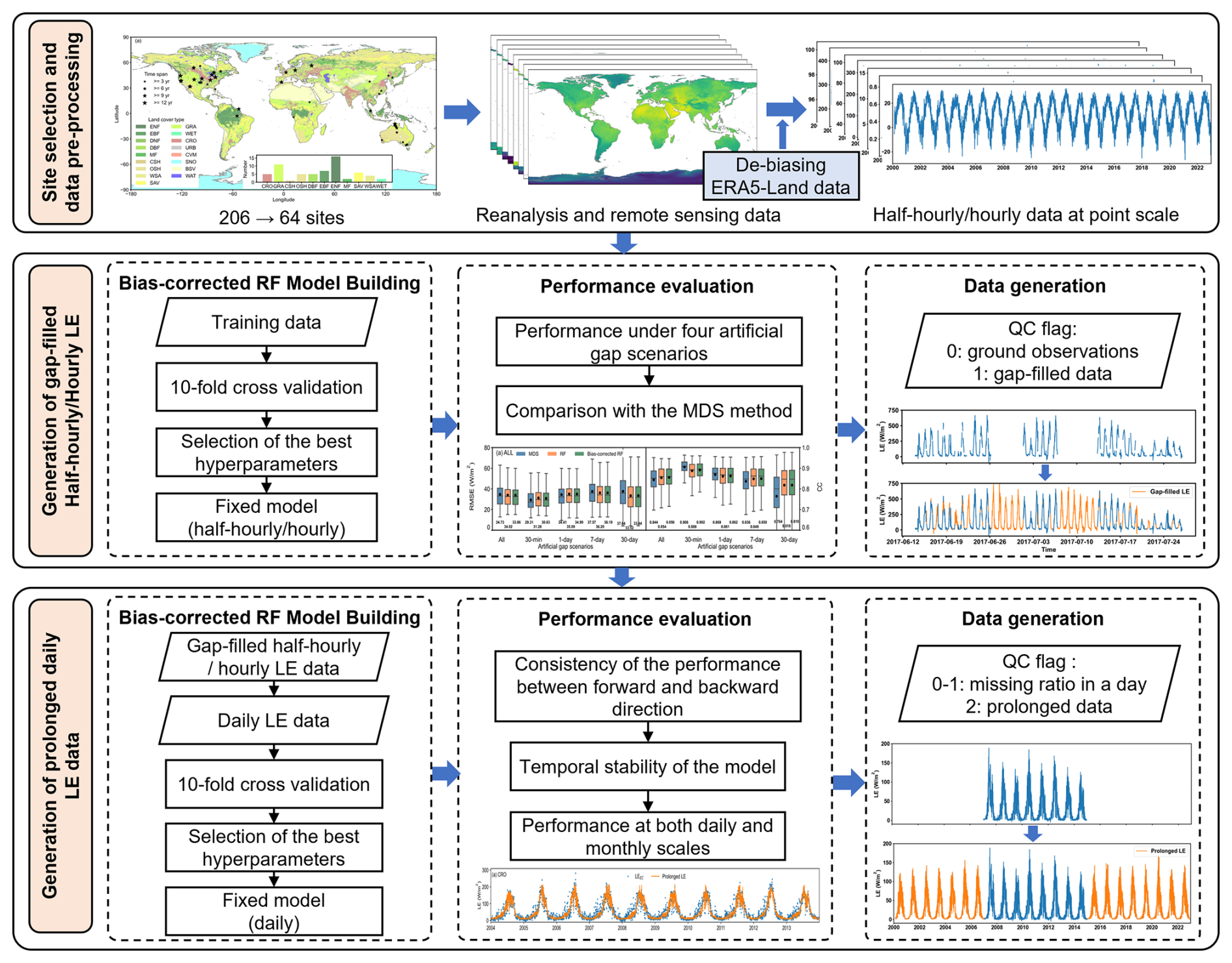
Figure 1 Schematic of the gap-filling and prolongation framework for LE_EC data.

3 Methodology

The gap-filling and prolongation framework for LE_EC data mainly includes three parts: site selection and data pre-processing, generation of gap-filled half-hourly or hourly LE data, and generation of prolonged daily LE data (Fig. 1). The details are described in this section.

3.1 Site selection and data pre-processing

3.1.1 FLUXNET2015 site selection

We selected 64 sites from 206 open-access FLUXNET2015 sites based on the following filtering criteria: (1) time span – sites must have ≥ 3 years of observations because sufficient temporal coverage is essential for reliable data prolongation; (2) missing data rate – sites must have ≤50 % missing data, so that there is adequate data availability for half-hourly or hourly gap-filling; (3) energy balance closure – we calculated the daily energy balance ratio (EBR) when there were ≥ 36 (18 for hourly data) valid observations in a day. The EBR values closest to 1 indicate the best agreement with the first law of thermodynamics, reflecting higher-quality surface energy data. Sites were retained for analysis only if more than 20 % of their observation days exhibited EBR values between 0.8 and 1.2. The EBR was calculated as follows:

$$\begin{array}{}\text{(4)}& \text{EBR}={\displaystyle \frac{{\sum }_{i=\mathrm{1}}^n(\text{LE}+H)}{{\sum }_{i=\mathrm{1}}^n(R_{\mathrm{n}}-G)}},\end{array}$$

where R_n, G, and H are the net radiation, soil heat flux, and sensible heat flux, respectively.

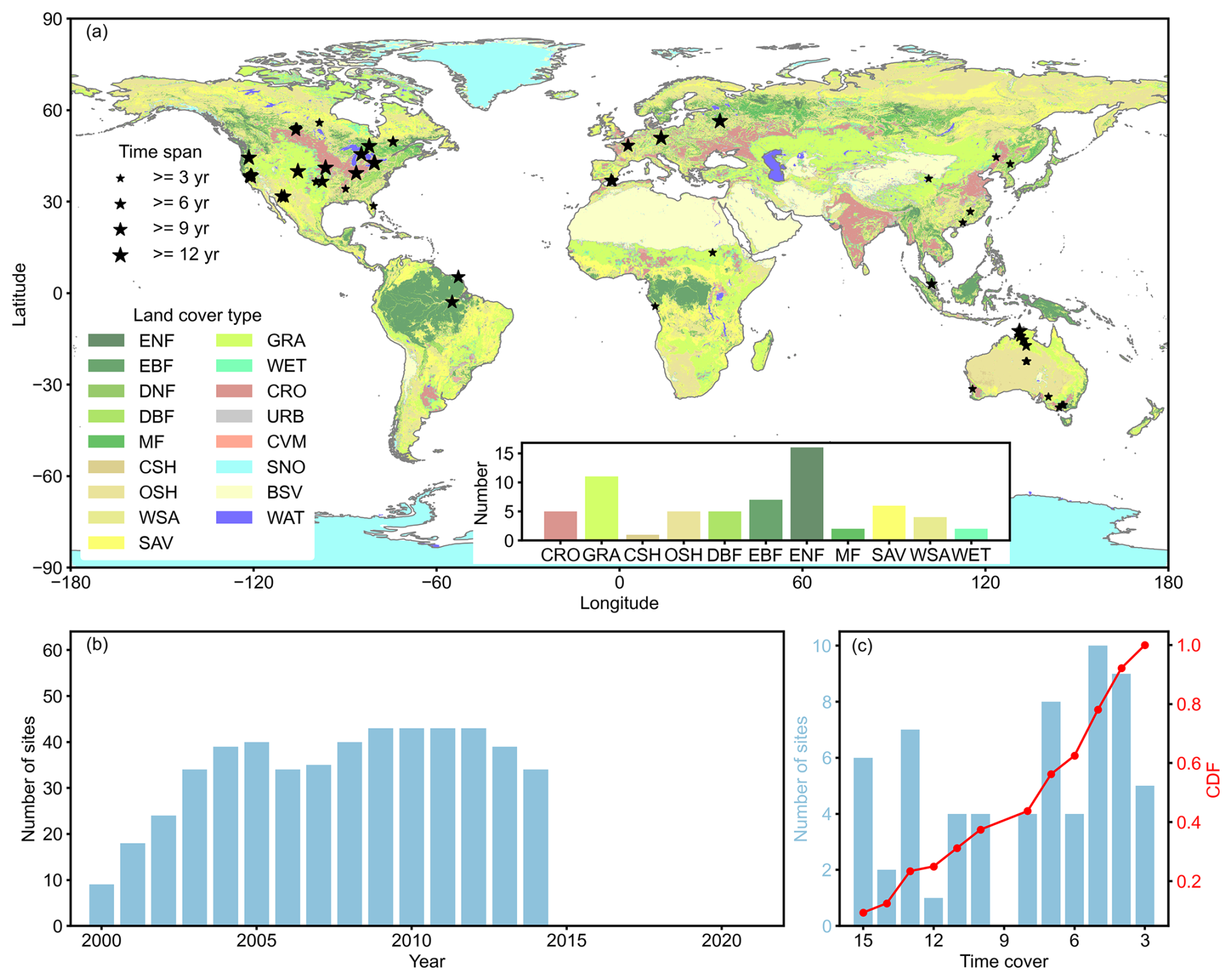
Figure 2 Global distribution (a) and information (b, c) of 64 selected FLUXNET2015 sites. The size of the star mark indicates the length of the data record. Panel (b) shows the number of sites in a year from 2000 to 2022. Panel (c) is the statistic of the length of observation periods for all sites.

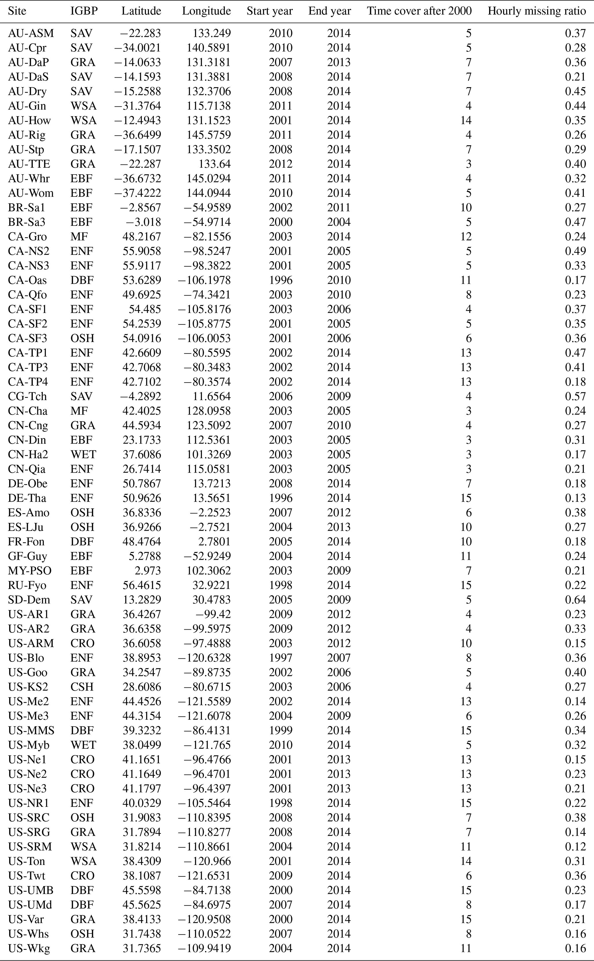
Notably, no sites in Africa fully met the specified criteria. Consequently, we selected two additional sites that substantially met the essential requirements. In total, 64 sites were selected (Fig. 2). These sites cover most regions, with 49 in the Northern Hemisphere and 15 in the Southern Hemisphere. Sites in Europe and the Americas have longer observation periods, while those in Asia and Oceania are shorter. The average duration of observations across all sites is approximately 8 years. Between 2000 and 2014, observations were available from approximately 10 to 40 sites per year. Moreover, these sites represent the majority of vegetated land cover types. For detailed site information, see Table A1.

3.1.2 Data pre-processing

We followed the same data pre-processing procedure as Li et al. (2024a). For the LE_EC data, non-observed values were filtered out based on quality control flags, with the remaining data used for training and testing datasets. The LE_EC data are reported at local time.

Reference variables, including TA, WS, RH, PA, SW_IN, LW_IN, and NDVI, were selected based on the Penman–Monteith (PM) equation (Monteith, 1965). These variables directly or indirectly influence the parameters in the PM equation and represent the most suitable variables for characterizing the meteorological and vegetated conditions affecting the ET process (Zhang et al., 2008; Mu et al., 2011; Li et al., 2024a). The PM equation is expressed as

$$\begin{array}{}\text{(5)}& {\displaystyle }& {\displaystyle }\text{LE}={\displaystyle \frac{\mathrm{\Delta }{R}_{\mathrm{n}}^{\ast }+\frac{\mathit{\rho }{c}_p\times \text{VPD}}{r_{\mathrm{a}}}}{\mathrm{\Delta }+\mathit{\gamma }\left(\mathrm{1}+\frac{r_{\mathrm{s}}}{r_{\mathrm{a}}}\right)}},\text{(6)}& {\displaystyle }& {\displaystyle }\text{VPD}=e_{\mathrm{s}}-e,\end{array}$$

where Δ is the slope of the vapor pressure curve, $R_{\mathrm{n}}^{\ast }$ the net available radiation at the evaporating surface, ρ the density of air, c_p the specific heat of air at constant pressure, VPD the air vapor pressure deficit, γ a psychrometric constant, r_s the surface resistance, and r_a the aerodynamic resistance.

Reference variables from ERA5-Land and MODIS were extracted as time-series data at point scale using Google Earth Engine (https://code.earthengine.google.com/, last access: 23 July 2025). Depending on the temporal resolution of LE_EC data records, the hourly time-series data from ERA5-Land were resampled to a half-hourly scale using linear interpolation, or maintained at an hourly scale. All timestamps were converted from UTC to local time to match the site-specific time zone. The NDVI data with a 16 d temporal resolution were resampled to a daily frequency using Savitzky–Golay filtering. The same value was then assigned uniformly for each day.

3.1.3 Debiasing the ERA5-Land data

To minimize mismatches between in situ and raster data, the time-series data from ERA5-Land were processed further. We followed a procedure similar to the official products (Vuichard and Papale, 2015) and corrected biases between ground observations and ERA5-Land using a linear correction method:

$$\begin{array}{}\text{(7)}& {\text{Ground}}_i=k_i\times {\text{EL5}}_i+b_i,\end{array}$$

where i means different variables, EL5 is the ERA5-Land data, and Ground is the ground observations from FLUXNET2015. These variables were filtered by quality control flags and only valid observations were used. The ground-observed vapor variable was VPD instead of RH for some sites. We transferred it to RH using the following equation:

$$\begin{array}{}\text{(8)}& \text{RH}=\left(\mathrm{1}-{\displaystyle \frac{\text{VPD}}{e_{\mathrm{s}}}}\right)\times \mathrm{100}\mathit{\%}.\end{array}$$

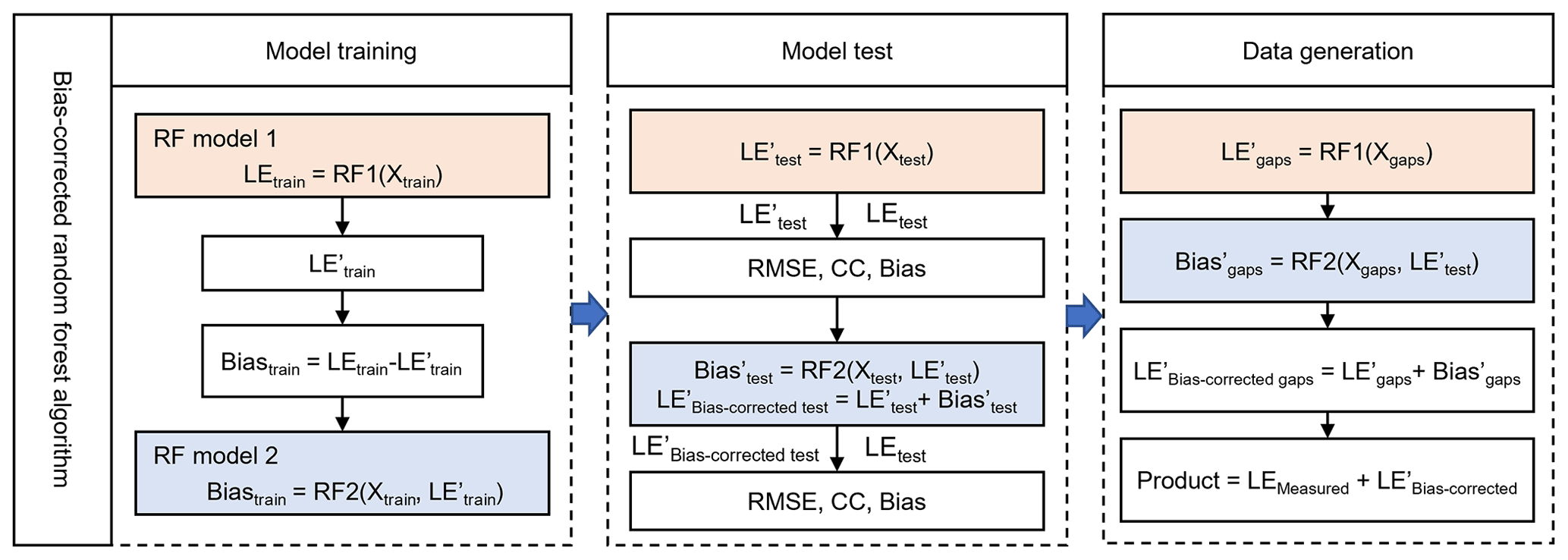
Figure 3 Schematic diagram of the bias-corrected RF algorithm. The subscript “train” indicates the training data; the subscript “test” indicates the test data. The subscript “gaps” indicates the data gap to be filled. LE^′ and Bias^′ indicate predicted values, whereas LE and bias indicate ground observations. X indicates the reference variables, including TA, WS, RH, PA, SW_IN, LW_IN, and NDVI. Prolonging daily data also has the same processing steps.

3.2 Generation of gap-filled half-hourly or hourly LE data

3.2.1 Bias-corrected random forest algorithm

The RF algorithm, used for both classification and regression tasks, is composed of multiple decision trees, and it combines their predictions to generate the final output (Breiman, 2001). Numerous studies have demonstrated the effectiveness of machine learning algorithms for gap-filling ground-based ET data (Moffat et al., 2007; Irvin et al., 2021; Mahabbati et al., 2021; Zhu et al., 2022; Li et al., 2024a). The RF algorithm is considered one of the most robust and efficient machine learning algorithms for replacing the traditional MDS algorithm and has significant potential for prolonging time series. However, there has been limited research on prolonging LE_EC time series using RF, and no corresponding datasets have been released. Although the performance of RF in flux data gap-filling has proven to be efficient, it still faces challenges such as overestimating lower values and underestimating higher values. Therefore, it is necessary to correct the bias. Here, we chose a novel bias-corrected RF algorithm (Zhang and Lu, 2012). It added a bias correction RF model to improve the performance compared with the original RF (Fig. 3). This algorithm has been used for studies such as drought monitoring (Feng et al., 2019; Wang et al., 2023). In this study, the bias-corrected RF model was adapted for processing flux data, and the detailed procedure of this bias-correction method is summarized in Fig. 3.

In the model training step we trained one model (including RF Model 1 and RF Model 2) for each site, resulting in a total of 64 models for the data gap-filling task. For each site, the data were randomly divided into two parts: the training dataset (80 % of the total dataset) and the test set (the remaining 20 %). To optimize model performance and avoid overfitting, we employed a 10-fold cross-validation method to determine the optimal combination of hyperparameters. For each site, the training and test dataset were generated 20 times, so we did the 10-fold cross validation 20 times and gained 20 hyperparameter combinations. We found that, for each site, the 20 hyperparameter combinations are almost the same. Therefore, we chose the hyperparameter combination based on two criteria: (1) achieving optimal model performance, and (2) exhibiting the highest frequency of occurrence across 20 experimental trials. Consequently, each site has a site-specific and unique hyperparameter combination. Finally, we used all valid LE observations to build the model. See Sect. 3.2.2 for details on how to split the training and test sets.

3.2.2 Artificial gap scenarios

The length of gaps in LE_EC data varied significantly, ranging from one single missing record to gaps exceeding 30 d. To fully evaluate the performance of our model we generated four gap-length scenarios, covering short to long durations: 30 min, 1 d, 7 d, and 30 d (Zhu et al., 2022; Li et al., 2024a). The artificial gaps for each scenario accounted for approximately 5 % of the total dataset, and all gaps collectively constituted the test set (20 %). After removing these artificial gaps, the remaining data (80 %) were used to train the model. Specifically, we used a sliding window approach to generate gap scenarios. If the valid observed data coverage within a window exceeded 50 %, the window was marked. The window automatically moved forward until this criterion was met, and no overlaps among marked sliding windows ensued. The sliding window size was initially set to 30 d. After completing one full round of marking, we randomly selected gaps accounting for 5 % of the total dataset, and these data were removed. The sliding window size was then reduced to 7 d and 1 d, and the process was repeated. Finally, we randomly removed 5 % of the half-hourly data to create the 30 min scenarios, ensuring five consecutive valid data points before and after each gap. To ensure robustness of the results we generated 20 different training–test sets and repeated the above steps 20 times for each site.

For comparison, we also used the MDS algorithm and original RF algorithm as the gap-filling algorithm of the framework. The core of the MDS algorithm is to use a sliding window approach to find similar meteorological conditions (Reichstein et al., 2005). It primarily uses SW_IN, VPD, and TA as reference variables. The larger the sliding window, the lower the confidence in the gap-filling results. To closely simulate the official data-production process, this study set the minimum thresholds for the three variables at 50 W m⁻², 5 hPa, and 2.5 °C, respectively. The MDS algorithm was implemented using REddyProc (R package, v.1.3.3).

3.3 Generation of prolonged daily LE data

Current mainstream ET products are predominantly available at daily and monthly scales (Zhang et al., 2019; Zheng et al., 2022; Miralles et al., 2025). Therefore, prolonging daily-scale ET data aligns best with current practical application scenarios.

3.3.1 Data generation

Following half-hourly/hourly gap-filling, we obtained continuous time-series data. These data were then aggregated from half-hourly/hourly to daily resolution, with the daily missing rate included as a QC flag. For data prolongation we employed the bias-corrected RF algorithm, maintaining the same model architecture and training procedure described in Sect. 3.2.1. During model training we trained one model for each site, selecting all data except those with a missing rate of 1 (completely missing) for model training. The 10-fold cross-validation method was used to determine the optimal hyperparameters. Ultimately, the seamless daily LE data from 2000 to 2022 were produced. The final product has been deposited at https://doi.org/10.5281/zenodo.13853409 (Li et al., 2024b) and can be downloaded publicly.

3.3.2 Experimental design for evaluating the prolonged data

Since the number of days with a missing ratio of 0 at the daily scale is extremely limited, we considered that daily data with a missing ratio below 10 % could serve as the test data.

The prolongation at the daily scale was conducted in two time directions: forward and backward. For example, one site has time cover from 2007 to 2014. Therefore, prolongation of 2000–2006 is the backward direction, and prolongation of 2015–2022 is the forward direction. We expect that the prolongation performance will be consistent in both directions. To validate the consistency of our method we adopted the following approach: for backward prolongation, the first $\mathrm{1}/\mathrm{3}$ of the data served as the test set, while the remaining $\mathrm{2}/\mathrm{3}$ was used for training; for forward prolongation, the first $\mathrm{2}/\mathrm{3}$ of the data was used for training, and the last $\mathrm{1}/\mathrm{3}$ served as the test set. We then compared the performance of both directions.

To assess the temporal stability of the model's performance as the prolongation period increased, we conducted experiments using two representative observation lengths: for sites with ≥ 8 years of observations, we used the first 8 years as the training set and the subsequent years as the test set. For sites with ≥ 3 years of observations, we used the first 3 years as the training set and the subsequent years as the test set.

3.4 Performance metrics

We selected four commonly used performance metrics, including the root mean square error (RMSE, W m⁻²), bias (W m⁻²), correlation coefficient (CC), and coefficient of variation (CV). The equations are as follows:

$$\begin{array}{}\text{(9)}& {\displaystyle }& {\displaystyle }\text{RMSE}=\sqrt{{\displaystyle \frac{\mathrm{1}}{n}}{\sum }_{i=\mathrm{1}}^n(p_i-o_i{)}^{\mathrm{2}}},\text{(10)}& {\displaystyle }& {\displaystyle }\text{bias}={\displaystyle \frac{\mathrm{1}}{n}}{\sum }_{i=\mathrm{1}}^n(p_i-o_i),\text{(11)}& {\displaystyle }& {\displaystyle }\text{CC}={\displaystyle \frac{{\sum }_{i=\mathrm{1}}^n\left(p_i-\stackrel{\mathrm{‾}}{p}\right)\left(o_i-\stackrel{\mathrm{‾}}{o}\right)}{\sqrt{{\sum }_{i=\mathrm{1}}^n{\left(p_i-\stackrel{\mathrm{‾}}{p}\right)}^{\mathrm{2}}{\sum }_{i=\mathrm{1}}^n{\left(o_i-\stackrel{\mathrm{‾}}{o}\right)}^{\mathrm{2}}}}},\text{(12)}& {\displaystyle }& {\displaystyle }\text{CV}={\displaystyle \frac{\mathit{\sigma }}{\mathit{\mu }}}\times \mathrm{100}\mathit{\%},\end{array}$$

where p_i and o_i are the values from prediction and observation, respectively; $\stackrel{\mathrm{‾}}{p}$ denotes the mean predicted value; σ is the standard deviation of the target data; and μ is the averaged value of the target data.

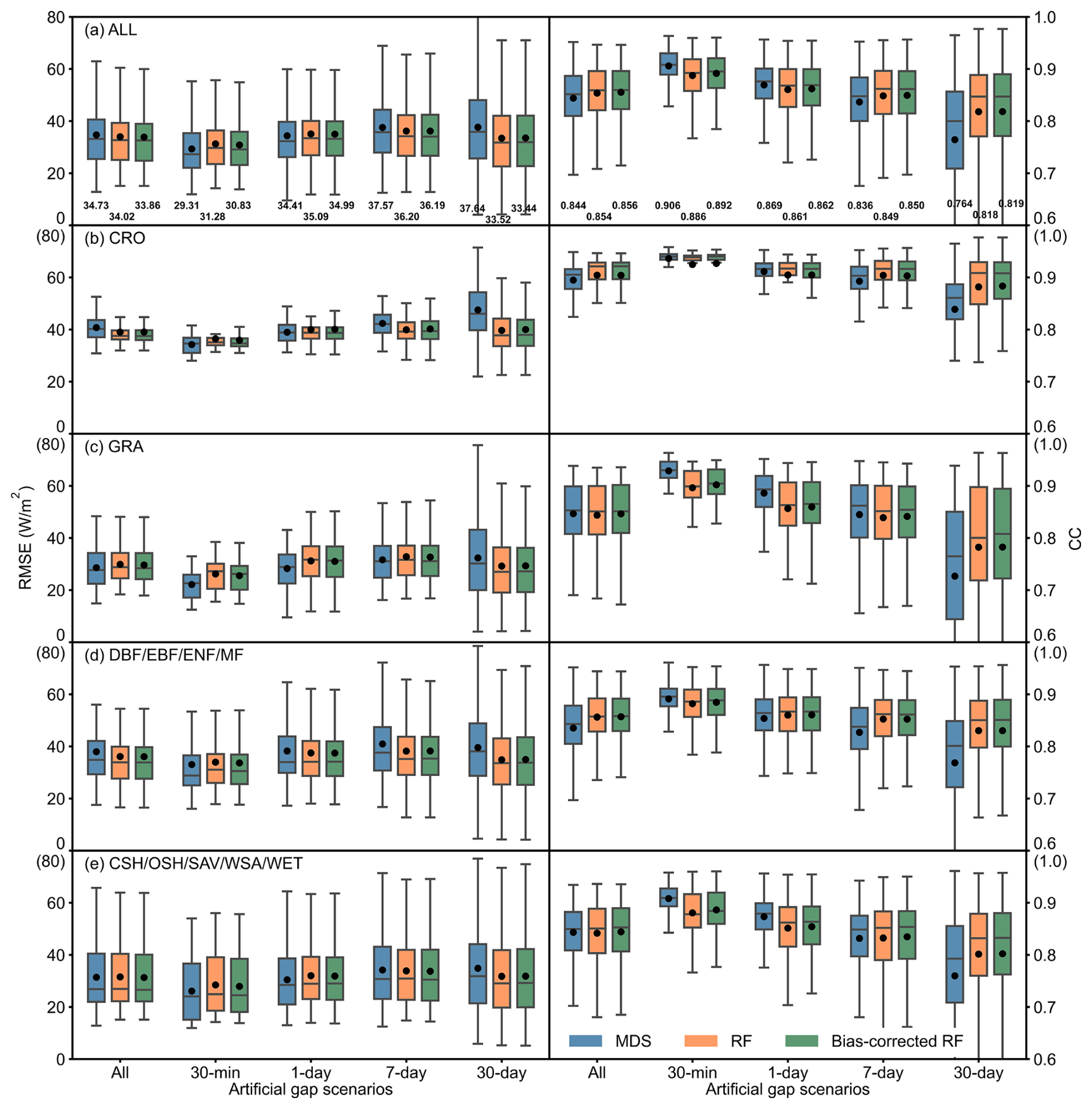
Figure 4 The gap-filling performance of three algorithms under different gap-length scenarios. The left panels show the results for the root mean square error (RMSE, W m⁻²) and the right panels show the results for the correlation coefficient (CC) between gap-filled values and observations. Different rows of the figure indicate different land cover types. The three horizontal lines of the boxes indicate the first quartile, median, and third quartile, and the black dots indicate the means. Data labels in this figure are the mean value of RMSE and CC. MDS: marginal distribution sampling. RF: random forest.

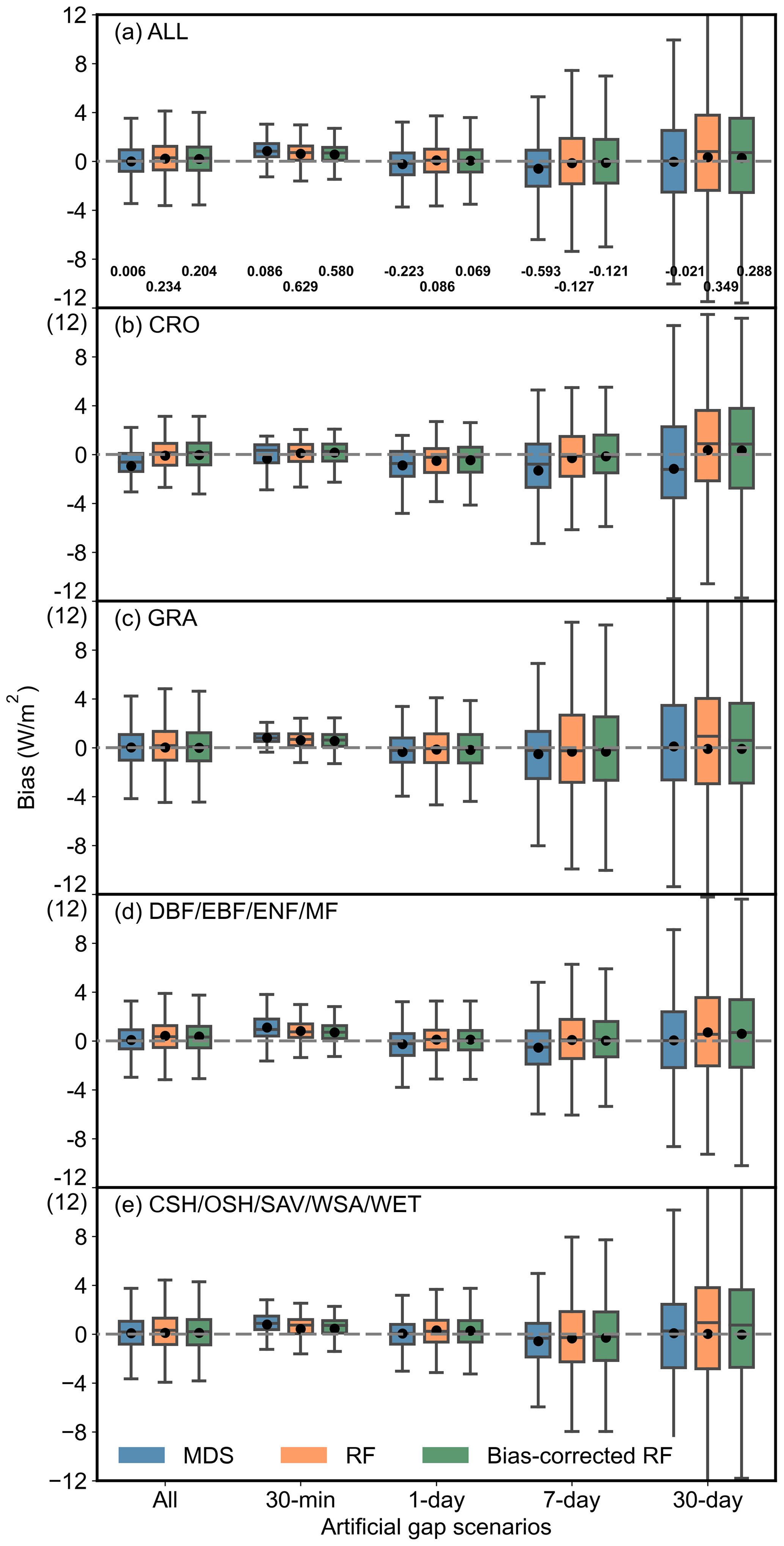
Figure 5 The bias between gap-filled values and observations of three methods under different gap-length scenarios. Different rows of this figure indicate different land cover types. The three horizontal lines of the boxes indicate the first quartile, median, and third quartile, and the black dots indicate the means. Data labels in this figure are the mean value of bias. MDS: marginal distribution sampling. RF: random forest.

4 Results

4.1 Evaluation of half-hourly or hourly gap-filled LE data

4.1.1 Gap-filling performance under different gap-length scenarios

We conducted a comprehensive evaluation of the gap-filling performance for three algorithms under artificially constructed gap scenarios, including the official algorithm (MDS), the widely used RF algorithm, and the novel bias-corrected RF algorithm. For each site and training–test combination, we computed RMSE, CC, and bias, and visualized the results in box plots (Figs. 4 and 5).

In general, the results indicate that the gap-filled data obtained using the bias-corrected RF are superior to those obtained using the official (MDS) algorithm, particularly outperforming it significantly for long gaps. The bias-corrected RF exhibits the best performance (33.86 W m⁻² and 0.86 in terms of mean RMSE and CC), with mean RMSE improvements of 0.87 and 0.16 W m⁻² compared to those of MDS and RF. As for the bias metric, Fig. 5 shows that as the gap length increases, the uncertainty increases and the bias-corrected RF provides more robust results.

For short gaps, the bias-corrected RF performs closer to MDS than the original RF. Specifically, the MDS performs exceptionally well, with mean values for RMSE and CC of 29.31 W m⁻² and 0.91, respectively, while the original RF performs the worst. The bias-corrected RF reduces the bias (0.45 W m⁻² in terms of RMSE), making its performance closer to that of MDS compared with the original RF. On the contrary, the performance of MDS deteriorates significantly with increasing gap length, aligning with previous findings (Foltýnová et al., 2020; Zhu et al., 2022; Li et al., 2024a). The bias-corrected RF achieves an 11.16 % lower mean RMSE (33.44 W m⁻²) than that of MDS (37.64 W m⁻²). The sliding window method makes MDS particularly struggle during the initial observation months, producing nearly identical values when early-month data are entirely missing (see Sect. 5.1 for a detailed analysis).

We further analyzed gap-filling results across different land cover types. Based on station count, land cover characteristics, and prior studies, we categorized the land surface types into four groups for analysis: CRO, GRA, DBF/EBF/ENF/MF, and CSH/OSH/SAV/WSA/WET. Overall, the bias-corrected RF outperforms the original RF and performs comparably to MDS across all land cover types. Notably, it achieves the most significant improvement in CRO, with a mean RMSE that is 4.26 % lower than that of MDS. This indicates that incorporating NDVI as a reference variable can better capture the seasonal dynamics of crops. In GRA and CSH/OSH/SAV/WSA/WET, the bias-corrected RF performs comparably to MDS, and both methods outperform the original RF. Across different gap-length scenarios the performance trends are consistent across land cover types. For short gap lengths the bias-corrected RF demonstrates performance similar to MDS, and both the RF and bias-corrected RF significantly outperform the MDS for longer gap lengths. Given that long gaps comprise 44 % of the FLUXNET2015 dataset, the bias-corrected RF can serve as a more reliable alternative to MDS for hourly-scale data gap-filling, yielding more robust results than those produced by MDS. Overall, the bias-corrected RF algorithm combines the superior performance of the original RF algorithm in long-gap-length scenarios, while providing corrections in cases where the original RF underperforms.

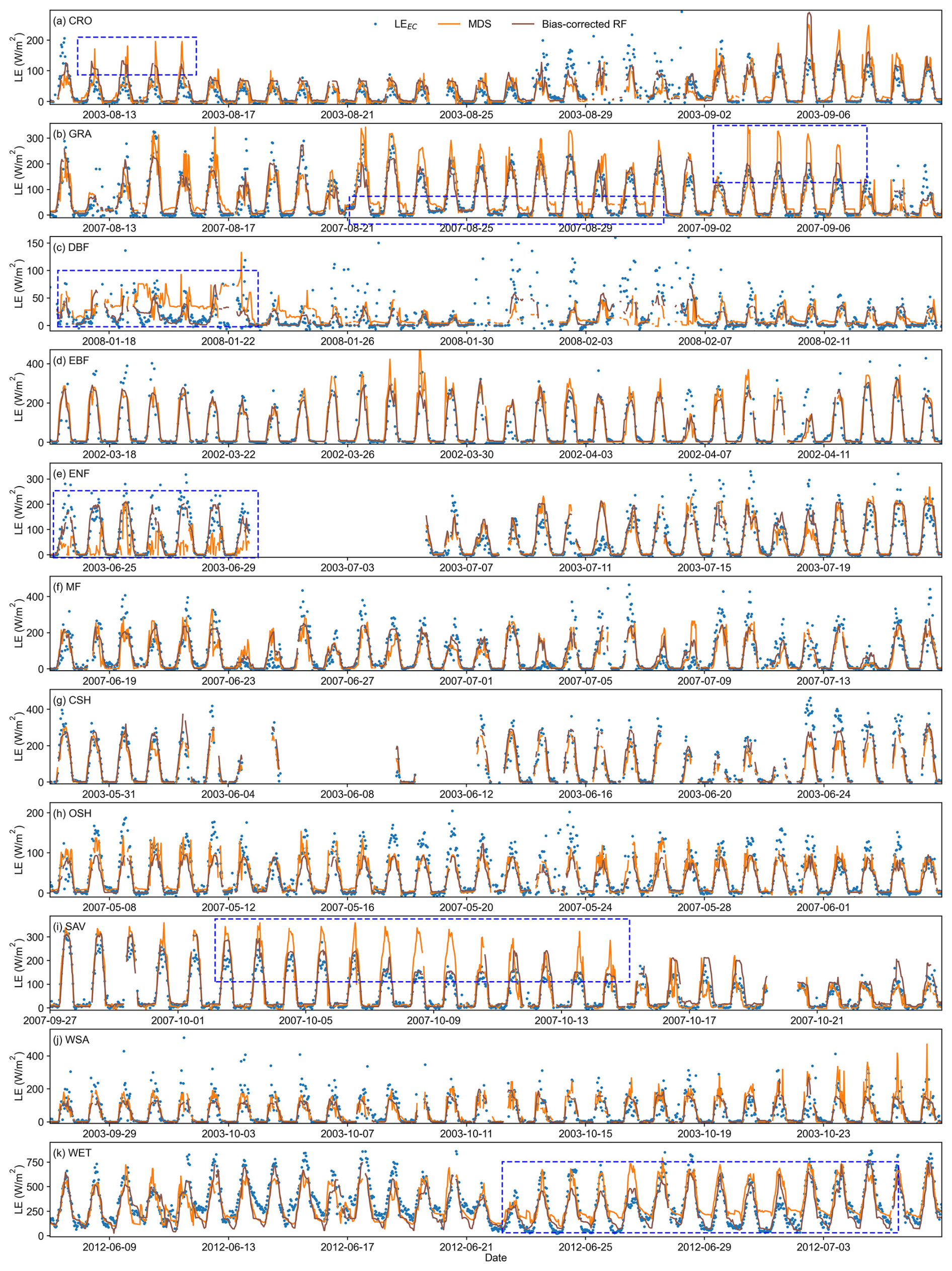
Figure 6 Time series of gap-filled results obtained from the bias-corrected RF algorithm compared to those from the MDS algorithm under an artificial 30 d gap-length scenario across different land cover types. The blue dashed boxes indicate scenarios where the MDS gap-filling results are significantly biased. The sites corresponding to each land cover type are: US-ARM, CN-Cng, FR-Fon, BR-Sa1, RU-Fyo, CA-Gro, US-KS2, ES-LJu, SD-Dem, AU-How, and US-Myb.

4.1.2 Examples of gap-filled data under artificial 30 d gap-length scenario

For the 30 d gap scenario, the bias-corrected RF algorithm performs better than the MDS algorithm in characterizing time series. As illustrated in Fig. 6, the bias-corrected RF demonstrates strong performance across all land cover types and provides a more accurate representation of daily periodic variations. Although minor biases persist in predicting certain extreme values, these are generally smaller compared to those produced by MDS. In contrast, MDS exhibits significant gap-filling biases across different land cover types, resulting in abnormal overestimations and underestimations (Fig. 6a, b, and i). In some cases it even fails to capture the daily variations of LE (Fig. 6e), while also distorting irregular LE changes (Fig. 6c).

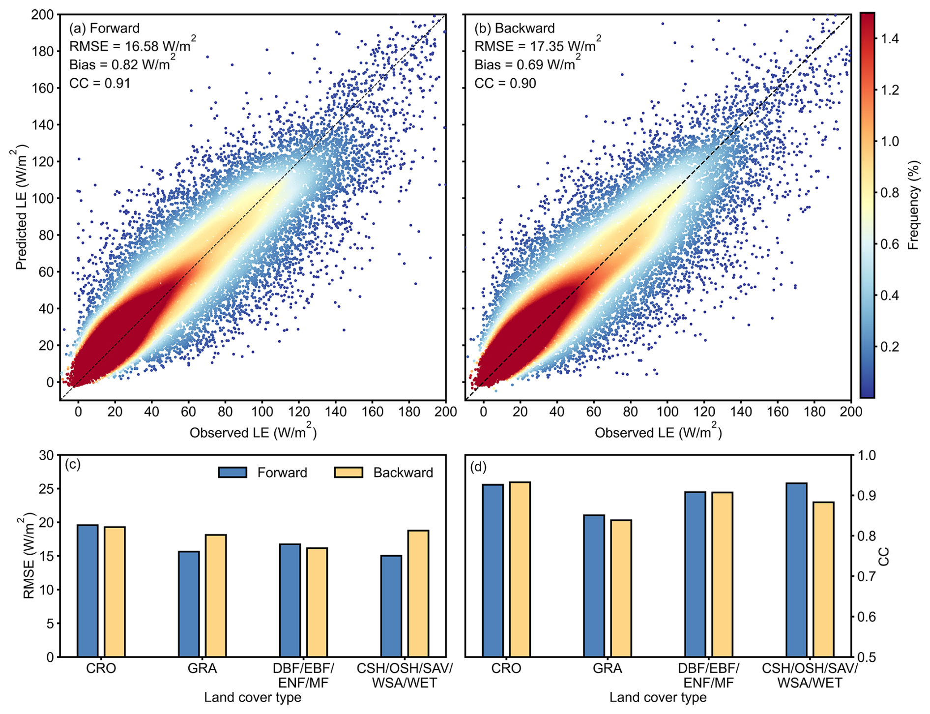
Figure 7 The consistency of forward and backward prolongation. (a) and (b) show scatterplots of predicted daily LE against observations for forward and backward prolongation, respectively. (c) and (d) are the specific performance of different land cover types.

4.2 Evaluation of daily prolonged LE

4.2.1 Consistency between forward and backward prolongation

As shown in Fig. 7a and b, the prolongation performance in both forward and backward directions exhibits high consistency. The results have good accuracy, with RMSE (CC) values of 16.58 W m⁻² (0.91) for forward and 17.35 W m⁻² (0.90) for backward. The slight difference may be mainly due to a higher volume of missing data in the first two-thirds of the data compared to the last two-thirds for sites of these land cover types (see Sect. 5.1). There are slight variations in prolongation results for different land cover types (Fig. 7c and d). Performance of CRO and DBF/EBF/ENF/MF is almost the same in both directions. Similar to the half-hourly data gap-filling, our results also demonstrate excellent performance in cropland, with a CC of 0.93 in both directions. GRA and CSH/OSH/SAV/WSA/WET perform slightly worse (2.46 and 3.74 W m⁻² higher) in the backward direction.

Figure 2b indicates that the need for forward prolongation is significantly greater than that for backward prolongation from 2000 to 2022. Therefore, the validation in the following sections will only focus on the forward direction.

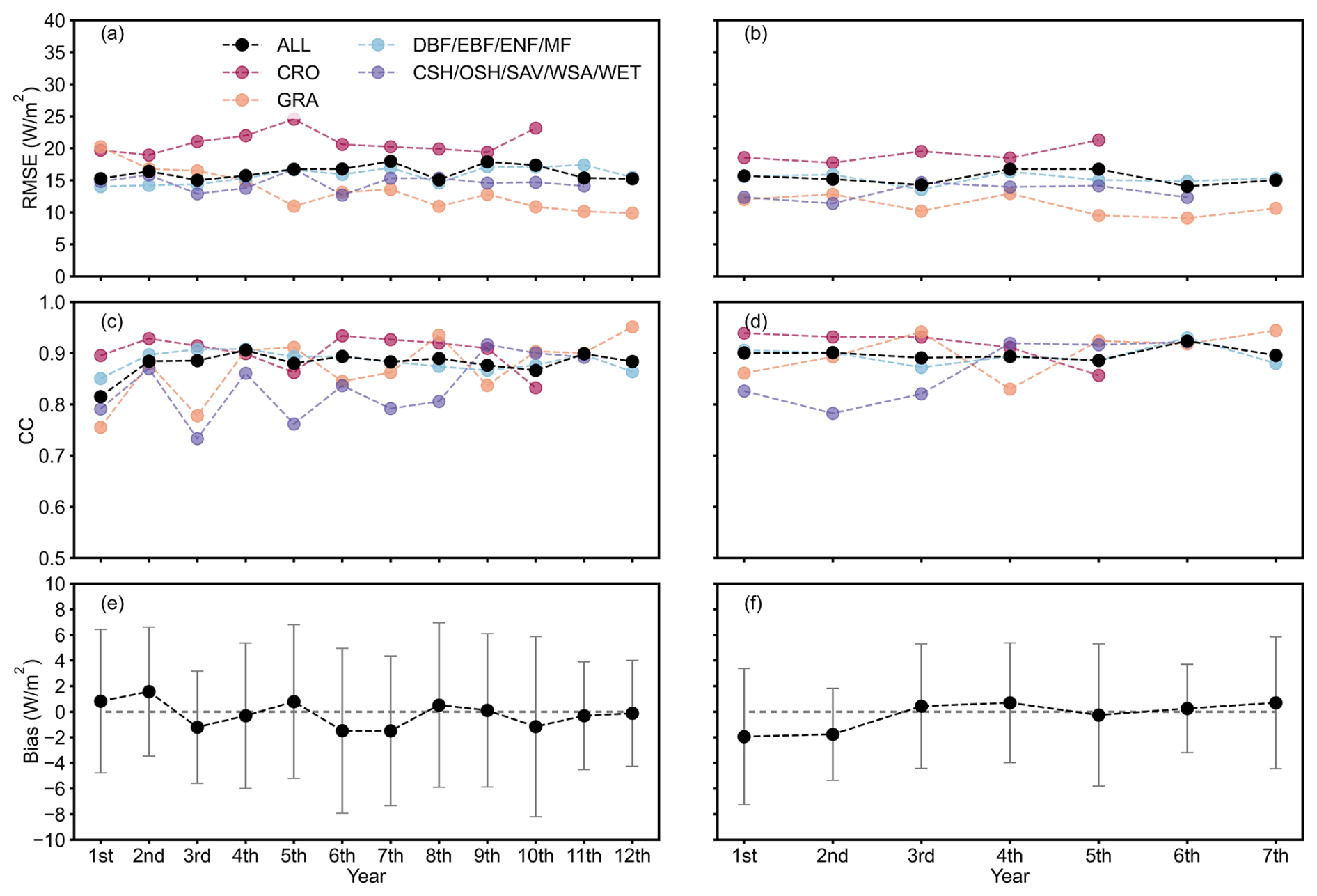
Figure 8 The temporal stability of the prolongation algorithm for different land cover types. (a), (c), and (e) show the median of RMSE, CC, and bias obtained from the model trained by the first 3 years data, respectively. (b), (d), and (f) show the median of RMSE, CC, and bias obtained from the model trained by the first 8 years data, respectively.

4.2.2 Temporal stability of the prolongation

We used data from the first 3 years and the first 8 years for training, and evaluated the prolongation performance for each subsequent year. Three years of data represents an extreme case of the minimum training data volume in this dataset, while eight years of data reflects a typical scenario within the dataset. Figure 8 shows that our prolongation results exhibit minimal performance degradation over time. The greater the amount of training data, the higher the temporal stability. Specifically, the model trained using the first three years yields CVs of RMSE and CC of only 3.29 % and 3.83 %, respectively. The model trained using the first 8 years yields CVs of RMSE and CC of only 3.24 % and 1.75 %, respectively. The bias fluctuates within a small range around zero each year, indicating that our estimation bias is relatively robust. For different land cover types, DBF/EBF/ENF/MF shows good stability, while GRA and CSH/OSH/SAV/WSA/WET show more noticeable fluctuations over time but do not experience significant performance degradation. Overall, our model demonstrates excellent temporal stability in both extreme and typical cases.

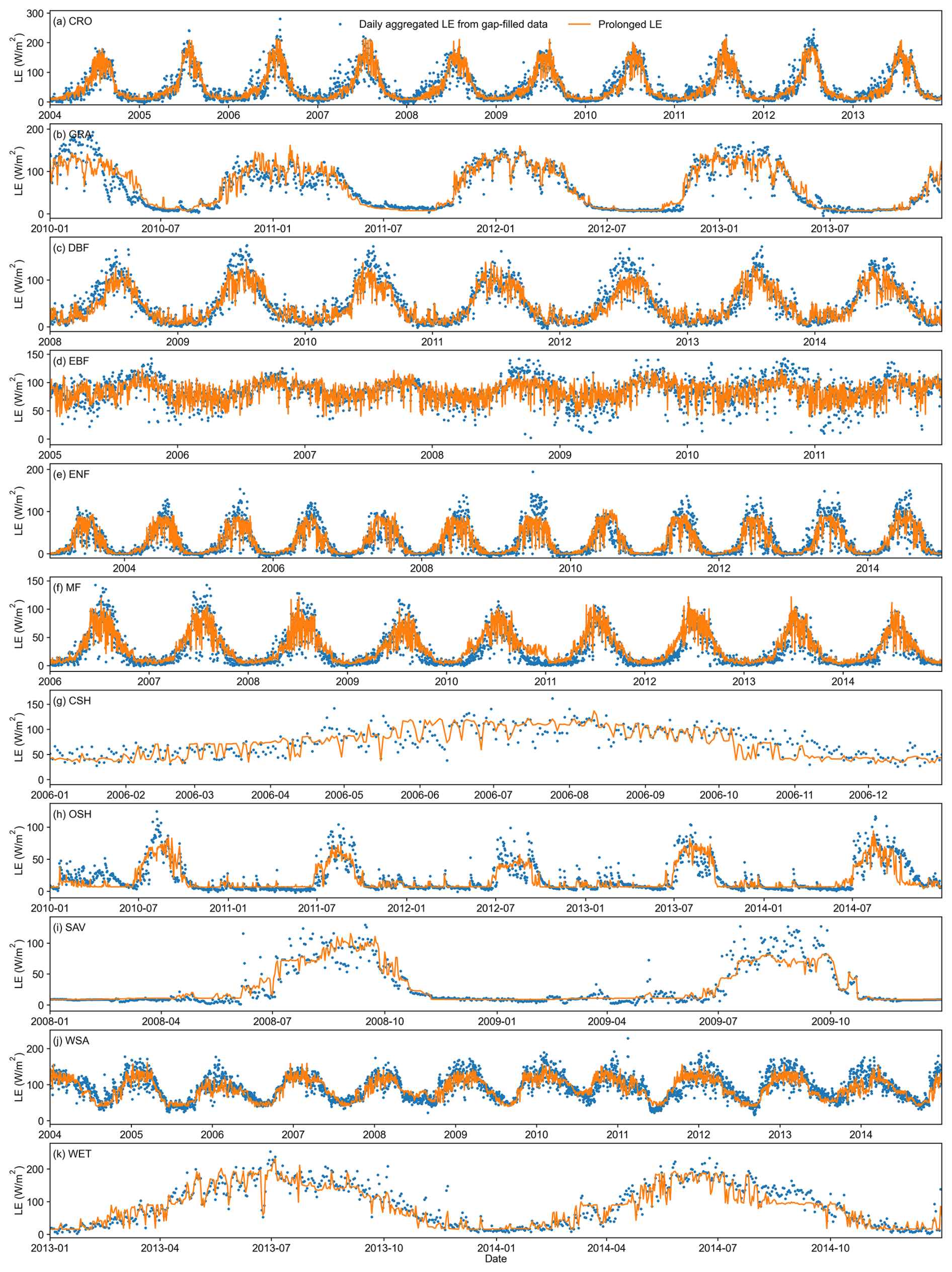
Figure 9 Time series of daily prolonged results obtained from the model trained using the first three years across different land cover types. The sites corresponding to each land cover type are: US-Ne1, AU-DaP, FR-Fon, BR-Sa1, RU-Fyo, CA-Gro, US-KS2, US-Whs, SD-Dem, AU-How, and US-Myb.

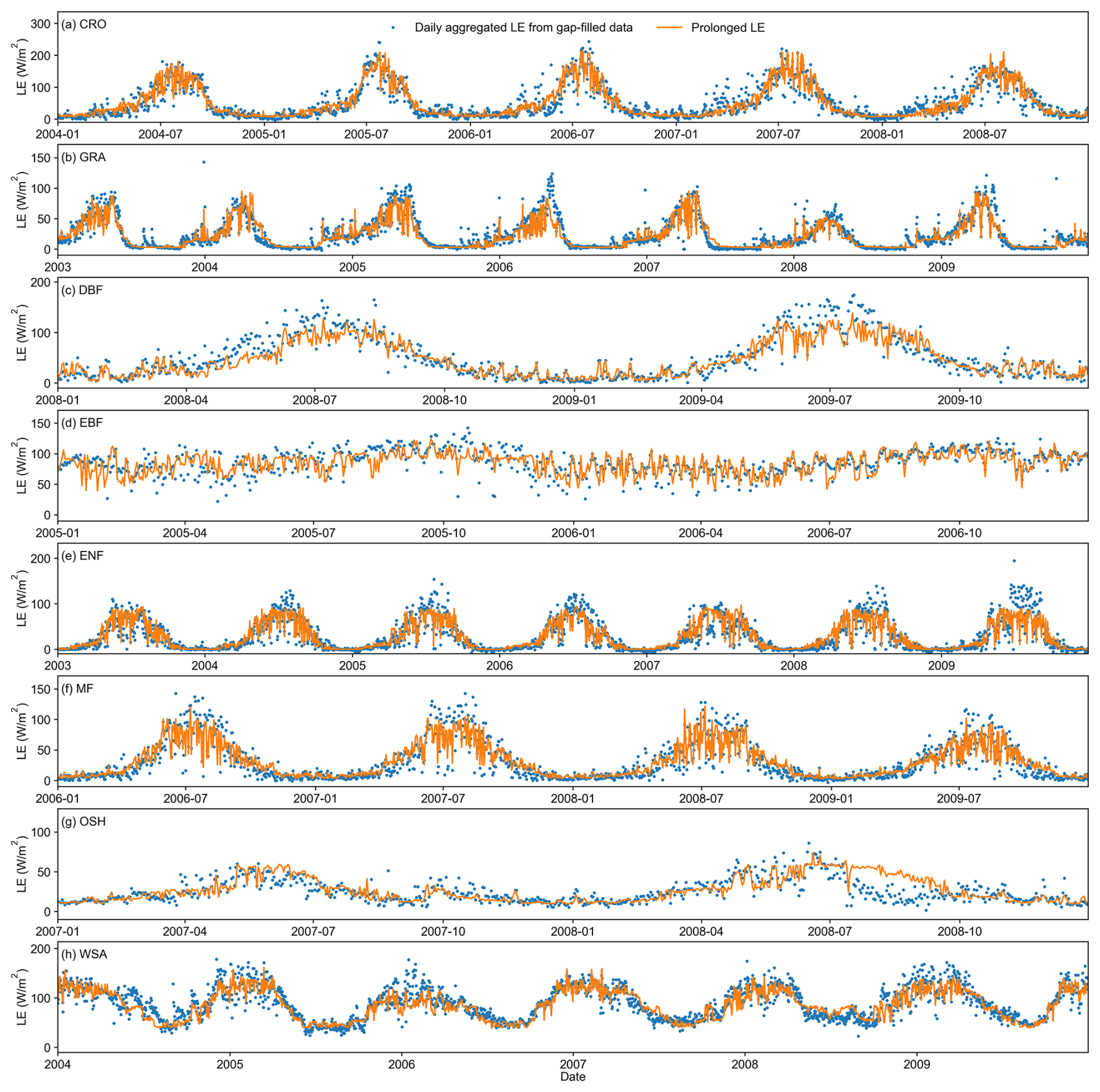
Figure 10 Time series of daily prolonged results obtained from the model trained using the first eight years across different land cover types. The sites corresponding to each land cover type are: US-Ne1, US-Var, FR-Fon, BR-Sa1, RU-Fyo, CA-Gro, ES-LJu, and AU-How.

4.2.3 Demonstration of daily- and monthly-scale prolonged time series

Due to the scarcity of days with a missing data rate below 10 %, we chose to compare the prolonged results from Sect. 4.2.2 with the daily data aggregated from the hourly gap-filled data. We plotted the results obtained in Sect. 4.2.2 as time series graphs and compared the prolonged results with the aggregated daily data from hourly gap-filled results. As shown in Figs. 9 and 10, our prolongation algorithm effectively captures the seasonal variation of LE, aligning well with hourly gap-filled results in both magnitude and trend. The model performs excellently in both extreme (3 year data) and typical (8 year data) cases, particularly for sites with CRO land cover type. For evergreen vegetation sites (ENF and EBF) and sparse vegetation sites (SAV and OSH), the lack of vegetation change information leads to unclear influencing factors on LE variation, resulting in underestimation of some extreme high values. However, our algorithm still performs well in capturing daily fluctuations.

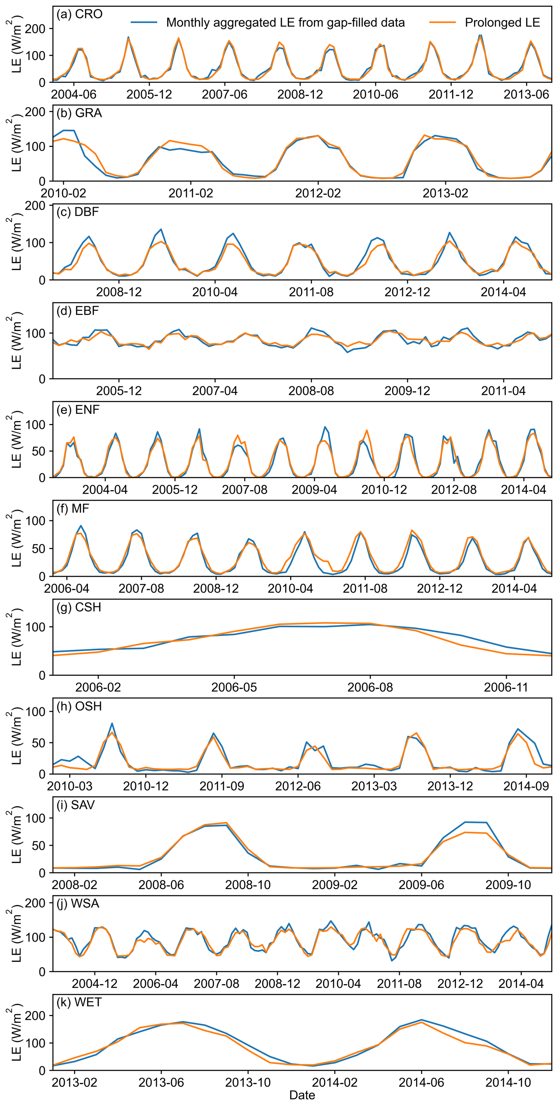
Figure 11 Time series of monthly aggregated results obtained from the model trained using the first three years across different land cover types. The stations corresponding to each land cover type are: US-Ne1, AU-DaP, FR-Fon, BR-Sa1, RU-Fyo, CA-Gro, US-KS2, US-Whs, SD-Dem, AU-How, and US-Myb.

Given that many global change studies focus on monthly scales, we aggregated the daily data to assess the performance. As shown in Fig. 11, the monthly scale results meet the requirements of related research. Both the trend and magnitude align well with hourly gap-filled results. The CRO sites match almost perfectly with the hourly gap-filled results, while the ENF and EBF sites, which performed slightly worse at the daily scale, accurately capture subtle fluctuations at the monthly scale.

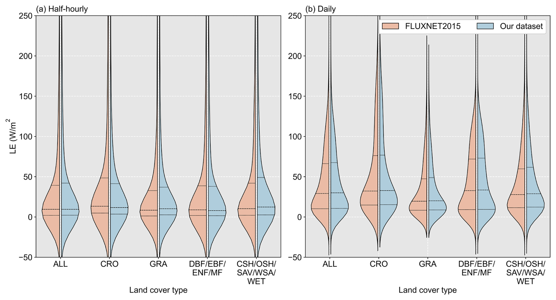
Figure 12 Distribution of gap-filled data at (a) half-hourly and (b) daily scales for our dataset and FLUXNET2015 dataset.

5 Discussions

5.1 Comparison between FLUXNET2015 and our dataset

After extensive analysis of the experimental design results in Sect. 4, we have demonstrated excellent gap-filling and prolongation performance at the methodological level. To evaluate our released dataset, we compared it with the official dataset from FLUXNET2015, as missing data in observations cannot provide verifiable truth. Figure 12 shows the data distribution results of gap-filled data at both hourly and daily scales for the two datasets. The results indicate a high consistency in data distribution between our dataset and FLUXNET2015. At the hourly scale, the median and quartiles of both datasets are nearly identical. For CRO, FLUXNET2015 exhibits slightly higher values compared to our dataset, while for GRA and CSH/OSH/SAV/WSA/WET its estimates are slightly lower. At the daily scale the consistency is even greater, with almost identical data distributions across all land surface types.

Figure 13 Scatterplot of LE data of our dataset against that of FLUXNET2015 dataset.

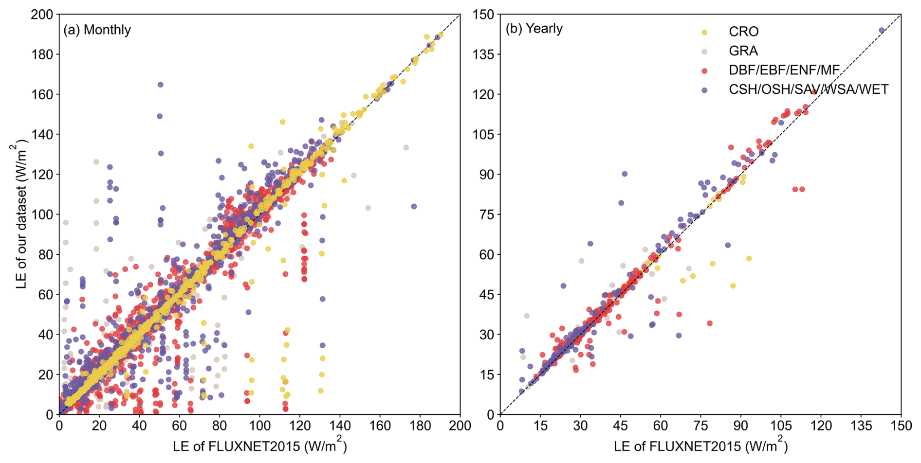
Additionally, we compared the differences between the two datasets aggregated to monthly and yearly scales. As shown in Fig. 13, the data from both datasets distributes along the 1:1 line at both monthly and yearly scales. Although some months and years exhibited discrepancies between the two datasets, it still demonstrates a high degree of consistency. Specifically, at the monthly scale we observed instances where some LE data of FLUXNET2015 show close values, while our predictions demonstrate clear distinctions. When aggregated to the yearly scale, these discrepancies manifested as outliers. This instance arises because many FLUXNET2015 sites experienced complete data loss for the first four to eight months (e.g., AU-ASM from January to August 2010, CA-Gro from January to July 2003, US-UMd from January to April 2007, among others). Due to the lack of neighboring information in the sliding window, the MDS algorithm struggled to provide effective gap-filling, resulting in nearly identical gap-filled values for those months. Consequently, these months could not be included in the usable data range, rendering the aggregated results at the yearly scale unreliable. In contrast, our algorithm can utilize the reference data for each specific moment to predict the corresponding LE, so we can provide more accurate gap-filling results.

5.2 Reference variable importance analysis

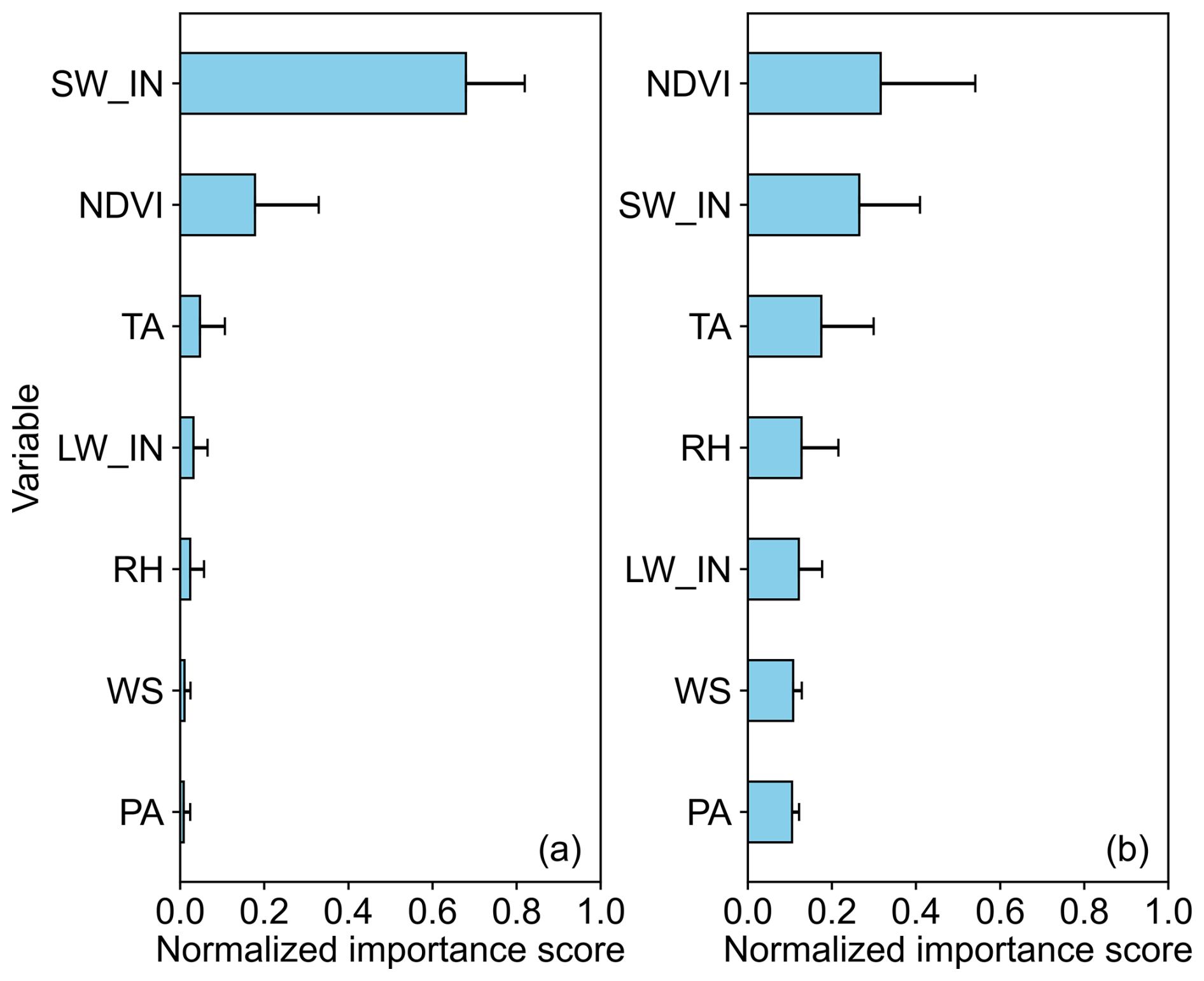
Figure 14 presents the results of reference variable importance using the permutation feature importance technique. Each input feature is randomly shuffled to calculate the performance deterioration. For half-hourly or hourly gap-filling, the order of variable importance is SW_IN > NDVI > TA > LW_IN > RH > WS > PA. Consistent with earlier research (Irvin et al., 2021; Zhu et al., 2022; Li et al., 2024a), SW_IN is the key variable that significantly influences LE variations across terrestrial ecosystems. It provides energy for the ET process. Throughout the day, SW_IN exhibits significant diurnal variation. NDVI is the second most important variable, but its influence varies between sites. This explains why the performance of the two land cover types in Sect. 4.2.3 is slightly inferior to that of other types. For sites with evergreen vegetation, seasonal changes in vegetation are not pronounced, making NDVI less effective in providing clear information to the model. For daily prolongation, the order of variable importance is different. The importance of SW_IN decreases significantly because daily LE variation is more closely related to NDVI, which reflects seasonal changes. Similar to the hourly scale, NDVI also shows inconsistencies between sites for the same reasons. Additionally, TA, as the third most important variable, provides critical information at sites dominated by soil evaporation. Variables like LW_IN, RH, WS, and PA hold comparable significance as minor factors, offering insights into the meteorological background conditions.

Figure 14 Variable importance for half-hourly or hourly gap-filling and daily prolongation.

5.3 Advantages and disadvantages

Our study presents several notable advantages. The bias-corrected RF shows better performance than the official MDS approach, especially for filling very long gaps (up to 30 d). Additionally, it allows for temporal prolongation, which the MDS method cannot achieve. Furthermore, our method enables the incorporation of a broader range of reference variables to establish a more robust non-linear relationship between LE and its drivers.

Compared to the FLUXNET2015 dataset, our hourly gap-filled data show improved quality and simpler implementation. The daily prolonged data provide extended temporal coverage (2000–2022) that is particularly valuable for ET modeling and global-scale studies. However, some limitations in terms of variable importance, sensitivity, and stability merit further discussion. The variable importance analysis (Sect. 5.2) indicates that our method exhibits strong sensitivity to SW_IN data for gap-filling and to NDVI for prolongation. While we implemented bias correction between ground observations and ERA5-Land data, potential quality issues in SW_IN and NDVI inputs may still affect final results. Future improvements could incorporate higher-quality input data with more stable biases to enhance result reliability.

6 Data availability

Our released dataset mainly contains four types of data:

• Half-hourly or hourly gap-filled data. The data were gap-filled using the novel bias-corrected RF algorithm. Filenames include “HH” for half-hourly or “HR” for hourly data. The time format follows FLUXNET2015 standards, with paired timestamps recorded in local time. The start and end times align with the observation period at each site. For QC flags, a value of 0 indicates observed data, while 1 indicates gap-filled data.

• Aggregated daily data. This daily dataset was aggregated from the gap-filled half-hourly data to a daily scale. The start and the end times match the observation period at each site. QC flags represent the percentage of valid hourly observations for each day.

• Prolonged daily data. This dataset provides the prolonged daily data using the novel bias-corrected RF algorithm. The seamless data spans 18 February to 31 December 2022. For the prolonged part, the quality flag is set to 2. The rest is consistent with the aggregated daily data.

• Aggregated monthly and yearly data. These datasets were aggregated from the prolonged daily data. QC flags indicate the proportion of days with > 90 % valid hourly observations per month or year. No distinction is made between prolonged data and completely missing daily data. The time span for the monthly data is March 2000 to December 2022, and that for the yearly data is 2001–2022.

All files are formatted as .csv files. NDVI and debiased reference variables from ERA5-Land are also provided in our released data. The product has been deposited at https://doi.org/10.5281/zenodo.13853409 (Li et al., 2024b) and can be downloaded publicly.

7 Conclusions

The current LE_EC data are increasingly insufficient to meet the growing demand for long time-series benchmark data to support climate change studies, model development, and product validation. To address these limitations in FLUXNET2015, we developed a gap-filling and prolongation framework for LE_EC data and established a benchmark dataset for ground-based ET (2000–2022) across 64 global sites. The results indicate:

• Hourly gap-filling: the novel bias-corrected RF algorithm demonstrates excellent performance, achieving a mean RMSE of 33.86 W m⁻². It improves the original RF algorithm's poor performance for short gaps, approaching the performance of the official algorithm (MDS). For long gaps, it significantly outperforms the MDS algorithm by 11.16 %. The algorithm more accurately predicts extreme values, thereby reducing result uncertainty compared to MDS. It performs consistently well across various land surface types, with the most notable improvements observed in cropland. Additionally, our gap-filled data distribution shows strong agreement with official products.

• Daily prolongation: our method exhibits robust performance in both forward and backward directions (16.58 and 17.35 W m⁻², respectively). The method shows slight variations in performance across different land surface types, with the best performance for cropland. In terms of temporal stability, our results maintain excellent performance under both extreme conditions (training with the first three years of data) and typical conditions (training with the first eight years of data). The time series effectively captures seasonal variations in LE, aligning well with observations.

• For hourly data gap-filling, SW_IN is the most important factor, while NDVI plays a decisive role in daily prolongation. In cases where the land surface is dominated by evergreen or sparse vegetation, the importance of NDVI significantly decreases.

Overall, our proposed gap-filling and prolongation framework for LE_EC data is robust and a benchmark dataset for global ET estimation based on FLUXNET2015 from 2000 to 2022 is established. It can provide essential data support for ET modeling, water–carbon cycle studies, and climate impact assessments.

Appendix A

Table A1 Site information.